SOCIO-ECONOMIC DISTANCE AND SPATIAL …web.pdx.edu/~crkl/WISE/SEAUG/papers/conley_topa_JAE02.pdfSOCIO-ECONOMIC DISTANCE AND SPATIAL PATTERNS IN ... If these non-physical metrics are

JOURNAL OF APPLIED ECONOMETRICSJ. Appl. Econ. 17: 303–327 (2002)Published online in Wiley InterScience (www.interscience.wiley.com). DOI: 10.1002/jae.670

SOCIO-ECONOMIC DISTANCE AND SPATIAL PATTERNS INUNEMPLOYMENT

TIMOTHY G. CONLEYa AND GIORGIO TOPAb*a Graduate School of Business, University of Chicago, USA

b Department of Economics, New York University, 269 Mercer Street, New York, NY, 10003, USA

SUMMARYThis paper examines the spatial patterns of unemployment in Chicago between 1980 and 1990. We studyunemployment clustering with respect to different social and economic distance metrics that reflect thestructure of agents’ social networks. Specifically, we use physical distance, travel time, and differences inethnic and occupational distribution between locations. Our goal is to determine whether our estimates ofspatial dependence are consistent with models in which agents’ employment status is affected by informationexchanged locally within their social networks. We present non-parametric estimates of correlation acrossCensus tracts as a function of each distance metric as well as pairs of metrics, both for unemployment rateitself and after conditioning on a set of tract characteristics. Our results indicate that there is a strong positiveand statistically significant degree of spatial dependence in the distribution of raw unemployment rates, forall our metrics. However, once we condition on a set of covariates, most of the spatial autocorrelation iseliminated, with the exception of physical and occupational distance. Racial and ethnic composition variablesare the single most important factor in explaining the observed correlation patterns. Copyright 2002 JohnWiley & Sons, Ltd.

1. INTRODUCTION

In this paper we examine the spatial patterns of unemployment in Chicago over two decades, 1980and 1990. We study unemployment clustering with respect to different economic distance metricsthat reflect the structure of agents’ social networks. Our goal is to characterize spatial patterns ofunemployment with respect to these metrics, in order to determine whether they are consistent withmodels in which agents’ employment status may be affected by information exchanged locallywithin their social networks.

There is considerable evidence that social networks are important for job search. A vast bodyof research in economics and sociology has shown that at least 50% of all jobs are found throughinformal channels, such as talking to one’s friends, family, neighbours, and social contacts ingeneral. In a study of 282 male professional and technical workers in the Boston area, Granovetter(1995) finds that about 57% of current jobs were found through personal contacts or referrals.Occupational contacts and weak ties were especially important.1 Corcoran et al. (1980) find verysimilar results using a much larger data set from the 1978 wave of the PSID. Montgomery (1991)

Ł Correspondence to: Giorgio Topa, Department of Economics-NYU, 269 Mercer Street, 7th floor, New York, NY, 10003,USA. E-mail: [email protected]/grant sponsor: C.V. Starr Center for Applied Economics, New York University.1 Two persons A and B have weak ties if agent A’s social network has very little overlap with agent B’s set of contacts.They have strong ties if they talk to roughly the same group of people.

Copyright 2002 John Wiley & Sons, Ltd. Received 11 May 2000Revised 19 April 2001

304 T. G. CONLEY AND G. TOPA

reports additional evidence and develops an adverse selection model in which informal hiring(through referrals) coexists in equilibrium with more formal hiring channels.

Such information exchange processes occurring within agents’ networks can generate observableimplications if the network structure is at least partially observable to the econometrician. Forexample, if social networks are geographic in nature, i.e. individuals talk mostly to those whoare physically nearby, then individuals’ outcomes will be related to their physical distance.A job-acquisition process that operated through such a network would generate clustering ofunemployment with respect to physical distance. Of course, social networks need not be strictlygeographic. Networks develop along other dimensions, such as race or ethnicity, religiousaffiliation, education. In addition, the information exchange between any pair of agents is likely tobe more productive (in terms of generating job offers) if the two agents are close in terms of theirrespective occupations. If these non-physical metrics are important, they will be systematicallyrelated to agents’ outcomes.

The underlying motivation for this research is to provide measures of spatial dependence inunemployment according to several metrics, in order to empirically evaluate competing economicmodels of behaviour. Local interaction models of information exchange and informal hiringchannels can be estimated by choosing parameters to match the observed spatial autocorrelationpatterns as a function of a given metric, via a Simulated Method of Moments or an IndirectInference procedure.2 The spatial implications of models of positive sorting of individuals acrosslocations, the spatial mismatch hypothesis, or a theory of unemployment that relies on thedistribution of skills across workers can also in principle be evaluated using the approach developedhere.

More generally, a better understanding of the likely components of socio-economic distancewill greatly facilitate the estimation of social interaction effects.3 Akerlof (1997) analyses atheoretical model in which social interactions are inversely related to social distance betweenagents. According to Akerlof, the concept of social proximity includes, but is not limited to,geography. In order to empirically evaluate such a model, the possible determinants of sociallocations need to be identified. Evidence from the sociology literature on social networks andlocal communities provides the motivation for the types of candidate metrics we consider. AsManski (1993) points out, using such direct evidence on the attributes that determine agents’reference groups is essential if one is to have any hope of estimating endogenous social effects.

In this paper, we construct several different metrics over Chicago Census tracts that attempt tocapture the physical as well as non-physical dimensions of social networks and job informationexchanges. These metrics are measures of physical distance, travel time, and the difference in ethnicand occupation distributions between tracts. Such metrics are often described by the sociologicalliterature as likely dimensions along which networks develop. To illustrate some of the differencesbetween metrics, we present a graphical illustration using a method called multidimensionalscaling.4 Comparisons of tracts’ relative distances under each metric are straightforward to make.

Upon construction of our metrics, we present nonparametric estimates of correlation across tractsas a function of specific metrics. First, we estimate these spatial Auto-Correlation Functions (ACFs)for unemployment rates themselves. Then, we estimate ACFs for residuals from a regression of

2 Topa (2002) uses this approach to estimate a structural local interaction model.3 Brock and Durlauf (2002) provide an excellent treatment of the identification issues and possible estimation strategiesthat are relevant for a general class of local interaction models.4 Mardia et al. (1979) provide a detailed description of this method.

Copyright 2002 John Wiley & Sons, Ltd. J. Appl. Econ. 17: 303–327 (2002)

SOCIO-ECONOMIC DISTANCE AND UNEMPLOYMENT 305

unemployment on a set of observable tract characteristics that are likely to affect the unemploymentrate of the area and to be spatially correlated due to the sorting of individuals across areas.5 Wecompare the two estimates to get an idea of whether the clustering with respect to a given metriccan be ‘explained’ by conditioning on these variables.

We also present non-parametric estimates of correlation as functions of combinations of metrics.For example, we estimate the auto-correlation of unemployment as a function of both physical andethnic distance and analyse the resulting two-dimensional auto-correlation surface. We estimatetwo-distance ACFs for several combinations of metrics, allowing us to examine the clusteringpatterns of unemployment according to the first metric, for the set of census tracts that are at agiven distance with respect to the second.

For any given ACF estimate, we provide a simple test of the hypothesis of spatial independence.We use a bootstrap method to generate an acceptance region for ACF estimates under the hypothesisof spatial independence. In addition to being easy to implement, these tests overcome the problemthat usual distribution approximations for local average estimates tend to overstate their precisionwhen the data is dependent. Our tests are also robust to measurement error in our metrics. Insofaras our measurements of distance are just proxies for the extent of connections between agents,they will certainly contain error.

Finally, we perform a covariance decomposition exercise, in order to determine which tract-level covariates contribute the most to ‘explaining’ the observed spatial correlation in the rawunemployment data. In particular, we provide a conservative and a liberal measure of the impactof specific subsets of regressors in explaining spatial correlation.

Our main results indicate that there is a strong positive and statistically significant degree ofspatial dependence in the distribution of raw unemployment rates, at distances close to zero, forall our metrics. The correlation decays roughly monotonically with distance. The two-metric ACFestimates offer some additional insights. When the physical, travel time, or occupation metric iscoupled with the ethnic metric, the latter drives most of the variation in spatial clustering: tractsthat are at a given ethnic distance exhibit a roughly constant degree of auto-correlation no matterwhat the physical, time, or occupation distance is between them. On the other hand, when physicalor travel time metrics are combined with distance in occupations, the estimated ACF surface isroughly decreasing in both distances.

The ACF estimates for the residuals from the regression of unemployment on a set of observabletract characteristics are quite flat. Once we condition on covariates, most of the spatial dependenceis eliminated. The only exceptions are the one metric ACF estimated using physical distance,and the two-metric ACF surfaces based on a combination of physical and occupational metrics.Therefore, it seems that most of the spatial clustering observed in the data may be driven bysorting of heterogeneous agents across locations.6

The results of our covariance decomposition exercise indicate that the overall situation isbest characterized as several variables each contributing some, rather than there being a singledominant explanatory variable. However, among these variables it is clear that the racial and ethniccomposition within each tract contributes the most to ‘explaining’ the spatial correlation presentin the raw data. Measures of human capital have a more limited impact and spatial mismatchvariables do not seem to play a role.

5 These variables include measures of human capital, age, race, housing values and neighbourhood quality, and so on.6 This, in turn, may be explained by a preference for living next to people with similar traits, or by a desire to internalizethe sort of local spillovers discussed here.



The methods in this paper may prove useful for data exploration and description of stylizedfacts in many other contexts. Our approach could be applied to other socio-economic outcomesof interest, such as participation in welfare programs, crime, dropping out of school, or teenagechildbearing. All that is required is measures of the relevant metric(s) describing the relationshipbetween units of observation—households, individuals, or Census tracts.

The remainder of this paper is organized as follows. Section 2 describes the data. Section 3discusses the different distance metrics used in our analysis, as well a comparison of theconfigurations implied by selected metrics via multidimensional scaling. The spatial econometricmodel is presented in Section 4. Section 5 reports the results of our ACF estimates for the differentmetrics and offers possible interpretations. Finally, Section 6 presents preliminary conclusions anddiscusses extensions of the current paper.

2. DATA

Most of the data come from the Bureau of the Census7 for the city of Chicago, at the tract level,for 1980 and 1990.8 There are 866 Census tracts in the city of Chicago, and they are grouped into75 Community Areas, which are considered to have a distinctive identity as a neighbourhood.9

Our unit of observation is the Census tract.In this paper we examine the clustering patterns of unemployment rates across Census tracts.

Our outcome variable is defined as the percentage of unemployed persons over the civilian labourforce (16 years and older). Unemployed persons are people who were neither ‘at work’ nor ‘witha job but not at work’ during the reference week used by the Census, and who were activelylooking for work during the last four weeks prior to the reference week.

As we mentioned above, we want to examine the spatial patterns of unemployment bothunconditionally and net of the clustering effect that may be simply due to sorting of individualsinto locations. Therefore, we control for a rather long list of observable neighbourhood attributes,that may be correlated with the probability of being employed, on the one hand, and may bedimensions along which people sort when deciding where to reside, on the other. We use threesets of covariates, listed in Table I and described below.

First, we define a set of sorting variables, i.e. variables that may affect the decisions by differenttypes of individuals to locate in a given area. These include average housing values in the Censustract, median gross rents, the fraction of vacant housing units in the area, the fraction of personswith managerial or professional jobs, the percentage of non-white persons, the percentage ofHispanic persons, a segregation index, and the number of persons per household.

Second, we consider variables that may be linked more directly to the probability of beingemployed. These include the percentage of persons with at least a high school diploma, thefraction of persons with at least a college degree, the age composition in the tract (to proxy forpotential experience), the fraction of females 16 years and older, and the percentage of males andfemales out of the labour force in the tract.

7 Summary Tape Files 3A.8 Travel times between locations were calculated using published CTA documentation.9 A set of tracts is defined as a Community Area if it has ’a history of its own as a community, a name, an awarenesson the part of its inhabitants of common interests, and a set of local businesses and organizations oriented to the localcommunity’ (Erbe et al., 1984, p. xix).



Table I. Census tract characteristics used as regressors

Sorting variables

Racial/ethnic composition Percentage of non-white personsPercentage of Hispanic persons

Others Segregation IndexAverage housing valuesMedian gross rentsFraction of vacant housing unitsPercentage of persons with managerial/professional jobsNumber of persons per household

Employability

Education Percentage of high school graduatesPercentage of college graduates

Others Percentage of persons 0–18 years oldPercentage of persons 0–24 years oldPercentage of persons 18–24 years oldPercentage of persons 16 years and older who are femalesPercentage of males out of the labour forcePercentage of females out of the labour force

Spatial mismatch

Median commuting time to work

Finally, there is a relatively large literature in urban and labour economics that discusses thespatial mismatch hypothesis. The literature aims at explaining the high unemployment levels inmostly black, inner-city neighbourhoods by local labour market conditions. The basic idea isthat during the 1970s and 1980s many jobs (especially low-skill ones in the service industry)have moved from central city areas to the suburbs. In addition, the contention is that there islow residential mobility and a certain degree of housing segregation for inner-city blacks. Forexample, it may be very costly for a black household to relocate to the suburbs in a mostlywhite neighbourhood, where the social capital provided by a black community would be missing.Several authors, such as Holzer (1991) and Ihlanfeldt and Sjoquist (1990,1991) have analysed thisissue empirically. By now, there is a certain consensus that physical proximity to jobs explains aportion of black/white unemployment differences, for instance. Therefore, we include the mediancommuting time to work for workers who reside in each tract as our measure of proximity to jobs.

3. DISTANCE METRICS

In this section we introduce four different distance metrics that we use in the remainder of thepaper to estimate spatial ACFs. In each instance, we try to motivate the particular choice ofmetric. It is important to keep in mind that our analysis is at the Census tract level, and not at theindividual agent level. Therefore, we do not trace out individual agents’ networks, but rather wedefine distances between pairs of tracts that attempt to reflect the dimensions along which socialnetworks are stratified. In so doing, we refer to a rich sociological literature that documents thepatterns of relations among agents. One unifying theme in the literature is that networks appearto be fairly homogeneous with regard to certain socio-demographic attributes.



3.1. Costs of Interaction

The first obvious choice for a distance metric reflects the locations of individuals on the physicalmap of the city. The underlying assumption is that the development and maintenance of socialcontacts is limited to some extent by physical distance and by transportation networks. In otherwords, we assume that there exist monetary and time costs of maintaining active social ties, thatare increasing in the physical distance between agents or in the travel time between locations ofresidence. This assumption implies that individuals are more likely to interact with people wholive physically close, and that the frequency of contact depends negatively on physical distanceor travel time.

Furthermore, local organizations at the neighbourhood level, such as churches, local businesses,neighbourhood clubs, schools or daycare centers, local sports or cultural associations, may lowerthe costs of interactions for individuals who reside within a neighbourhood or in adjacent areas,thus fostering social ties and facilitating information exchanges at the local community level.

There is a legitimate concern that physical distance may have become less and less important inshaping social networks, as many interactions take place between people who reside in differentneighbourhoods or even cities. High residential mobility and the availability of communicationtools such as the telephone or the Internet weaken the constraints that geographic space imposeson communities.10

However, there is some evidence that suggests that physical distance still plays an importantrole. In a study of Toronto inhabitants in the 1980s, Wellman (1996) finds that a surprisingly highfraction of interactions took place among people who lived less than 5 miles apart. The study askedrespondents (egos) to name a set of persons (alters) with whom they had active social ties, andrecorded the place of residence of respondents and alters, as well as the frequency of interactionswithin each ego–alter pair. The data show that about 38% of yearly contacts in all networks tookplace between ego–alter pairs that lived less than 1 mile away. Roughly 64% of all contacts tookplace between agents who lived at most 5 miles away.

In a Detroit study that used a 1975 survey of about 1200 residents, Connerly (1985) states that41% of respondents had at least one third of their Detroit friends residing within one mile. Guestand Lee (1983) perform a similar analysis for the city of Seattle, using the notion of CommunityArea. Using a sample of roughly 1600 residents, they find that for about 35% of the respondents atleast half of their friends resided in the same local community, whereas for about 47% of them atleast a few of their co-workers lived in the same area. More relevant to this paper, Hunter (1974)reports that out of roughly 800 Chicago residents interviewed during 1967-8, about 49% said thatthe majority of their friends resided in the same local community.11 Therefore, identifying socialcontacts with agents who live physically nearby seems like a reasonable approximation for one ofthe dimensions of social networks.

One important qualification is that such studies do not tell us anything about the content ofthese contacts: ideally, we would like to restrict our attention to networks whose primary contentis the information exchange about job openings. But one aspect reported by Wellman (1996) isencouraging. He observes that ties with one’s neighbours are weaker (in the sense specified in

10 There is a considerable debate among sociologists on whether the notion of a local physical community has lost allmeaning. See Wellman and Leighton (1979) and Connerly (1985).11 The exact definition of a local community roughly coincides with that of a Community Area, discussed earlier inSection 2.



Section 1) than ties with friends or kin. It is precisely this kind of ties that is more conducive togenerating useful information about jobs (see Granovetter, (1995)).

We use two different metrics to represent costs of interaction: physical distance and travel time:

ž Physical distance. PDij is the ‘as the bird flies’ distance in kilometres between the centroidsof tracts i and j. This metric is rather rough, as it does not take into account physical barriers,such as rivers or highways. It may also be worth while to examine variations of this metricthat take into account the population size or density in each census tract. The distribution ofpairwise distances across tracts using this metric is skewed to the right, and varies between about200 metres and almost 45 kilometres. The median distance is roughly 11 kilometres.

ž Travel time distance. TDij is the travel time distance (in minutes), using public transportation(CTA), between the centres of the Community Areas in which tracts i and j are located. Traveltimes were calculated from CTA timetables published in 1997 and reflect best-case travel times.12

The median travel time is 50 minutes and the distribution varies between zero and 120 minutes.

3.2. Race and Ethnicity

Even casual observation suggests that personal networks may be stratified along specific socio-demographic attributes, such as race, ethnicity, religious affiliation, language, age, gender, educa-tion levels. In other words, agents are likely to draw a disproportionate share of their social contactsamong sets of people that are very similar to themselves. This tendency is denoted as inbreeding,or homophily, among sociologists. Economists, on the other hand, refer to this phenomenon aspositive sorting, or assortative matching.13

But how exactly widespread is positive sorting within agents’ personal networks? There issome evidence that it is very strong among immigrant communities (see e.g. Light et al., 1993).The strongest evidence, however, comes from the 1985 General Social Survey. This study, begunin 1972, is an annual14 survey of the attitudes and behaviours of Americans on a wide varietyof topics. The 1985 edition included a module on social networks of 1534 individuals, drawnas a nationally representative sample. Respondents were asked to name people with whom they‘discussed important matters’. Several characteristics of these alters were then collected, amongwhich their age, sex, education, race, ethnicity, and religious affiliation.

Marsden (1987, 1988) has used the GSS data in order to analyse the question of assortativematching. The results indicate that personal networks are quite homogeneous along severaldimensions. In particular, network homogeneity with respect to race and ethnicity is very high.Only 8% of the respondents reported alters with any racial or ethnic diversity (both between egoand alters, and among alters). In addition, racial and ethnic heterogeneity of alters is only 13% ofthe total racial and ethnic heterogeneity among respondents.

Marsden (1988) then looks specifically at ego–alter pairs, and decomposes the cell frequencies(e.g. the relative frequency of black–black pairs over all the ego–alter pairs) into a portion that isdue to purely random matching (based on the marginal distributions of the race/ethnic categories

12 We hope that travel times during the 1980s are not very different from current ones. We tried as much as possible notto consider new lines that were opened in the mid-1990s.13 See Becker and Murphy ‘The sorting of individuals into categories when tastes and productivity depend on thecomposition of members’, unpublished manuscript’, for example.14 The GSS produced surveys annually in 1973-8 and 1983-93. Since 1994, it has been conducted every two years.



among respondents and alters), and a portion that is due to positive sorting. It turns out that thestrongest level of association, over and above random matching, takes place for the race/ethnicityattribute.15 For example, the chance of observing a black-black tie is 4.2 times higher than thatgenerated by pure random matching, given the relative proportions of the different racial andethnic categories in the population.16

Since our study is based on aggregated data and not on individual network data, we would liketo incorporate the positive sorting feature of social networks into a distance metric, that considerstwo tracts with very similar ethnic compositions to be close. The objective is to track more closelythis important dimension along which personal networks are structured. We propose the followingmetric to take into account racial and ethnic attributes:

ž Race and ethnicity distance. EDij is the Euclidean distance between the vector ei of percentagesof nine races and ethnicities17 present in tract i and the corresponding vector ej in tract j:

EDij D√√√√ 9∑

kD1

�eik � ejk�2

Thus two tracts with exactly the same racial and ethnic composition will be considered to be atracial and ethnic distance zero. Two tracts with extreme racial and ethnic compositions (e.g. oneis 100% Italian whereas the other is 100% Polish) will have a maximal racial/ethnic distance of100

p2. As is well known, Chicago is a very segregated city: the distribution of ethnic distances

is quite bimodal, with modal distances roughly at zero and 140 in both years.

3.3. Occupations

The last distance metric that we propose focuses on the informational content of social interactions.From our unemployment perspective, not all contacts are meaningful. We would like to keep trackof those social ties that are more likely to convey useful information about job openings, or togenerate referrals. For example, if agent A is a graphic designer and agent B is a doctor, evenif they appear in each other’s personal network it is unlikely that they would communicate anyuseful information about jobs to each other.

Again, there exists a certain amount of evidence on this. For example, Schrader (1991) uses asurvey of about 300 middle-level managers in the context of the US specialty steel industry. Hefinds strong support for the hypothesis that information flows quite freely through professionalnetworks. Granovetter (1995) reports that a significant fraction of tips on job openings comes frombusiness acquaintances and social contacts with similar occupations.

Therefore, we think it may be relevant to construct a distance metric between pairs of tracts thatis based on the within-tract distribution of occupations, in order to take into account the potentialusefulness of the informational content of social networks. We propose the following:

15 Marsden also considered age, gender, education, and religion. All these attributes exhibit a statistically significantpositive degree of assortative matching, over and above random matching.16 The same statistic is 2.9 for Hispanics, 3.1 for Asians, 2.6 for Whites.17 We use the percentage of Black, Native American, Asian and Pacific Islander, Hispanic, White, German, Irish, Italian,and Polish persons 16 years and older in each tract.



ž Occupational distance. ODij is the Euclidean distance between the vector oi of percentages ofworkers in 13 different occupations in tract i and the corresponding vector oj in j:18

ODij D√√√√ 13∑

kD1

�oik � ojk�2.

The interpretation of this metric is analogous to that of the race/ethnicity one: tracts with similaroccupation proportions are close. The distribution of occupational distances is skewed to the rightand varies between 2 and 124 in 1980, between zero and 141 in 1990. The median is 22 and 24in the two years.

3.4. Combinations of Distance Metrics

According to the definition of the racial/ethnic metric, or the occupational metric, two tracts aregoing to be at zero distance if they have the same racial/ethnic (or occupational) composition,even though they are located at the opposite physical ends of the city. This may not be entirelysatisfactory. One might think that the appropriate social distance metric, in order to identify whois more likely to talk to whom, is some combination of physical distance (or travel time) andracial/ethnic or occupational distance. Thus areas with exactly the same ethnic composition but atthe opposite ends of the city may interact less than areas with slightly different ethnic compositionsbut much closer geographically.

In order to take this possibility into account, we also estimate ACFs of unemployment as afunction of pairs of metrics. In this case, the estimated correlation between any two tracts will bea function of their distances with respect to both metrics. We can then examine how unemploymentclustering depends on different combinations of the two distances. Consider, for example, physicaland racial/ethnic distance. Fixing racial/ethnic distance at a level close to zero (say 20), and tracingthe ACF as a function of physical distance alone, one can get an idea of how spatial correlationvaries with physical distance, conditional on ethnic distance being equal to 20. Several possibilitiesmay arise. The ACF may decay monotonically in both directions, or be flat with respect to onemetric and only vary with the other.

We consider several pairs of distances.19 We look at racial/ethnic and occupational metricstogether and take combinations of the two types of geographic distance with racial/ethnic metricon the one hand, and with the occupational metric on the other hand. Thus we estimate thefollowing combinations of different metrics: physical and racial/ ethnic distance; physical andoccupational distance; travel time and racial/ethnic distance; travel time and occupational distance;and racial/ethnic and occupational.

18 The occupations are: executive, administrative, and managerial; professional specialty; technicians; sales; administrativesupport; private housheold; protective service; other service; farming, forestry, and fishing; precision production, craft, andrepair; machine operators, assemblers, and inspectors; transportation and material moving; handlers, equipment cleaners,helpers, and labourers.19 We avoid dealing with more than two metrics simultaneously because the performance of our local average techniquedeclines rapidly with an increase in the number of metrics simultaneously considered. This is another version of thewell-known problem of local averages suffering from a ‘curse of dimensionality’.



3.5. Comparison of Economic Distance Metrics

This subsection describes differences in relative locations of tracts under each of our metrics.We use a method to visually represent our constructed metrics as a configuration of points onthe plane, and compare this configuration to a map of tracts’ physical locations. Specifically, weuse a method called multidimensional scaling (MDS) to construct a configuration of points intwo dimensions whose interpoint distances approximate those for a given metric. Essentially, ouralgorithm constructs a configuration using the first two principal components of a standardizedversion of a distance matrix. Of course the MDS configuration is unique only up to a choiceof location and orientation, so we can only compare relative distances under each metric.20 Agoodness of fit statistic for the MDS configuration is available that can be roughly interpretedas the percentage of the variation in original distances captured by the fitted configuration. It isroughly analogous to the percentage of variance explained by the first two principal componentsof a covariance matrix.21

We plot the first tract in each of the 75 community areas to give an idea of these configurationsunder various metrics. Fifteen of these tracts are labelled with their community name so thatchanges in relative positions and clustering of these tracts can be examined. These areas are ArmourSquare, Austin, Bridgeport, Clearing, Dunning, Englewood, Gage Park, Hyde Park, Lincoln Park,Loop, Morgan Park, Rogers Park, South Chicago, South Shore, and Uptown.

The physical locations of the tracts are depicted in Figure 1. The origin on this map is centred atthe geographic centre of the points, near the Bridgeport neighbourhood. The vertical and horizontalaxis represent deviations in kilometres from the centre. The axes are not labelled, however, in orderto emphasize that relative distances between tracts are the objects of comparison across metrics,units will vary. The goodness of fit statistic for this configuration is virtually one, since the cityof Chicago is not large enough for the curvature of the earth to matter.

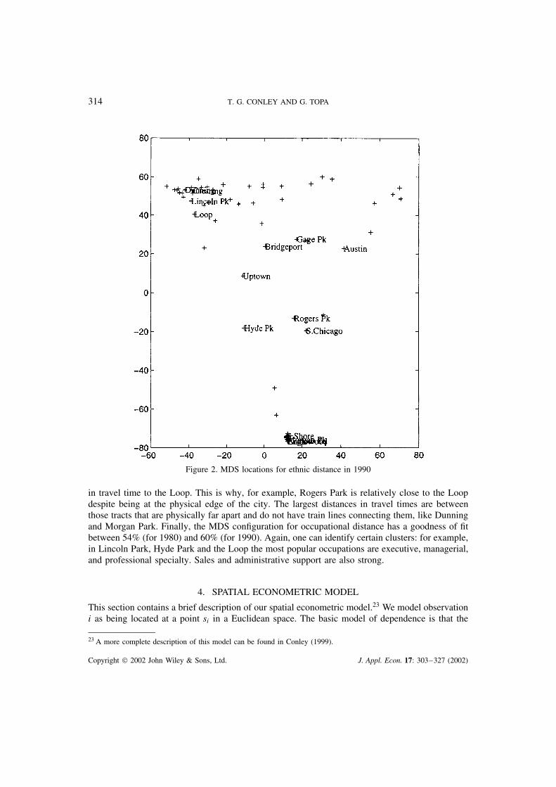
The MDS configuration for our measure of ethnic distance in 1990 is presented in Figure 2.This configuration captures almost all the variation in the ethnic metric, having a goodness offit statistic of 96% in both 1980 and 1990. The clustering of community areas is striking. Pre-dominantly minority areas such as South Shore, Englewood, and Morgan Park are clustered atthe bottom of Figure 2. These three Community Areas have a proportion of black persons thatranges between 97% and 100% in 1990. On the other hand, the cluster composed by Clearing,Dunning, Lincoln Park, and the Loop is predominantly white: in these Areas, whites make upbetween 87% and 98% in 1990. The ethnic composition in these clusters is remarkably stableacross the two Census years.22 Relatively few neighbourhoods had a mixed composition, such asHyde Park (because of the residents affiliated with the University of Chicago) or Gage Park andAustin (that went from being predominantly white in 1980 to having a slight Hispanic majorityby 1990).

The MDS configurations for travel time and occupational distance are available from the authorsupon request. The MDS configuration for the CTA travel time metric has a goodness of fit statistic

20 To facilitate comparisons, we have translated and rotated each fitted configuration to line up (to the extent possible)with that based on physical distance using a method called Procustes rotation. See Mardia et al. (1979) for a completeexplanation of this procedure.21 A brief description of MDS and this goodness of fit statistic is contained in an Appendix available from the authorsupon request. See also Mardia et al. (1979) for a thorough exposition.22 Both Clearing and Dunning have a significant presence of persons of Polish origin. This presence is very stable ataround 15% in both years.



−10 −5 0 5 10−25

−20

−15

−10

−5

0

5

10

15

20

25

Hyde Pk

Rogers Pk

Uptown

Loop

Austin

S.Shore

Bridgeport

Englewood

Gage Pk

Lincoln Pk

S.Chicago

Dunning

Morgan Pk

Clearing

Armour Sq

Figure 1. MDS locations for physical distance

of 36%. The reason for this relatively poor fit is that there are many locations across Chicago thatare close to being equidistant in terms of travel time via public transportation. Thus many pointsare equidistant under this metric, making it difficult to represent in a low-dimensional Euclideanspace. Neighbourhoods that lie on elevated train lines that radiate from the centre city are close



Figure 2. MDS locations for ethnic distance in 1990

in travel time to the Loop. This is why, for example, Rogers Park is relatively close to the Loopdespite being at the physical edge of the city. The largest distances in travel times are betweenthose tracts that are physically far apart and do not have train lines connecting them, like Dunningand Morgan Park. Finally, the MDS configuration for occupational distance has a goodness of fitbetween 54% (for 1980) and 60% (for 1990). Again, one can identify certain clusters: for example,in Lincoln Park, Hyde Park and the Loop the most popular occupations are executive, managerial,and professional specialty. Sales and administrative support are also strong.

4. SPATIAL ECONOMETRIC MODEL

This section contains a brief description of our spatial econometric model.23 We model observationi as being located at a point si in a Euclidean space. The basic model of dependence is that the

23 A more complete description of this model can be found in Conley (1999).



distance between observations’ positions, corresponding to their economic distances, characterizesthe dependence between their random variables. If observations i and j are close, then their randomvariables, say Xsi and Xsj, may be very highly correlated. As the distance between si and sj growslarge, Xsi and Xsj become closer to being independent.

Formally, we assume that our vector of variables Xs is stationary and satisfies regularityconditions in Conley (1999).24 Stationarity means that the joint distribution of Xs for any collectionof locations fsigm

iD1 (i.e.{

Xs1, Xs2, . . . , Xsm

}) is invariant to shifts in the entire set of locations

fsigmiD1. So, for example, the covariance of Xsi and Xsj is a function of si � sj. Furthermore we

assume that this covariance is a function of distance, not the direction of the vector si � sj:

cov�Xsi , Xsj� D f�jjsi � sjjj� �1�

We will use estimates of this spatial covariance function to describe the covariance of variablesas a function of distances.

To estimate the spatial autocovariance function in equation (1), we use a non-parametricestimator of the spatial autocovariance function. The estimator is essentially that proposed byHall et al.(‘On the non-parametric estimation of covariance functions’, unpublished manuscript,1992). The autocovariance at distance υ is estimated by a local average of cross-products of de-meaned observations that are close to υ units apart. Letting Dij D jjsi � sjjj, we estimate f�υ�with:

Of�υ� DN∑

iD1

N∑jD1

WN[jυ � Dijj]�Xsi � X��Xsj � X�

where X is the sample mean of X, and the weight function WN�Ð� is normalized to sum to one.In other words, we run a kernel regression of �Xsi � X��Xsj � X� on Dij. We require WN�Ð� to bea function of sample size that will concentrate its mass at zero as the sample becomes arbitrarilylarge at an appropriate rate. Thus, in large samples, the spatial covariance at distance υ will beestimated by an average of cross-products of only those observations that are arbitrarily close toυ units apart and Of will be consistent.

We will also estimate a generalization of this model that effectively allows us to considertwo different distance metrics. To do this, we can simply interpret each observation’s position asreflecting two metrics. For example if s1,i corresponds to the physical location of observation iand s2,i describes its ethnic composition, then we could index this observation by

si D[

s1,i

s2,i

]

Now, rather than restricting covariances to depend on the distance between si and sj we can allowthem to depend on distances between these two components:

cov�Xsi , Xsj� D f�jjs1,i � s1,jjj, jjs2,i � s2,jjj� �2�

24 The assumption of stationarity can be relaxed to allow non-explosive processes that have covariances that vary overspace. In this case our covariance function can be interpreted as an average of non-stationary covariances. The foremostregularity condition is that the process is mixing, that Xs and Xr become asymptotically independent as the distancebetween s and r goes to infinity.



Covariances here can depend on distance according to both metrics. We estimate this more generalcovariance function with a nonparametric regression as above. Estimates of (2) will be kernelregressions of �Xsi � X��Xsj � X� on two different measures of distance between observations iand j.

4.1. Testing Spatial Independence

We take a slightly unusual approach to conducting a test of whether there is spatial independence.Instead of using a limiting distribution of Of to test the implication that there is zero spatialcorrelation, f�υ� D 0, we plot an acceptance region for the specific null hypothesis of spatialindependence. Then our hypothesis test can be done by simply observing whether our pointestimate of f lies inside the acceptance region.

To compute an acceptance region for the hypothesis of spatial independence we employ a simplebootstrap techinque. We hold the sample locations fixed and simulate draws from a distributionwith the same stationary (marginal) distribution as our data but with spatial independence. To dothis simulation, we just sample with replacement from the empirical marginal distribution of ourvariables. For each of these bootstrap samples, which by construction are spatially independent,we can calculate a bootstrap estimate of f exactly as we had done for the original data. For eachvalue of υ we take an envelope containing, say, 95% of our bootstrap estimates to give us anapproximate acceptance region for the hypothesis of spatial independence.

We prefer this bootstrap method to tests based on limiting distributions for reasons beyondits simplicity. Tests based on the limiting distributions for our local average estimates of fwill tend to be unreliable in the presence of spatial dependence. Because the estimator relieson local averages, estimates of asymptotic variances will be the same as if the data were spatiallyindependent. There is evidence that such asymptotic approximations can be very misleading intime series applications of local average methods to data with a high degree of dependence (seee.g. Robinson 1983; Pritsker, 1996). Since, a priori, we expect there to be significant dependencebetween observations we want to avoid overstating the information in our sample by using theseestimators to deliver pointwise standard errors. Furthermore, we want to entertain the possibilitythat our economic distances are measured with error. In this case, our estimator Of will recover aweighted average of the true autocovariances. The positive weights will be an unknown functionof measurement errors and this will make using a limiting distribution to construct standard errorsdifficult. However, our bootstrap still computes a valid acceptance region for the null of spatialindependence for the resulting statistic.

5. ACF ESTIMATES

In this section, we first present ACF estimates for each of our metrics, as well as for pairs ofmetrics. Then we present a simple decomposition exercise aimed at investigating which sets ofvariables are most important in describing patterns of spatial correlation. We end this sectionwith a summary of our findings and a discussion of what they tell us about the nature of socialinteractions.



5.1. One-metric Spatial ACF Estimates

We now report the results of our spatial ACF estimates for each metric separately. TheseACF estimates are formed using the kernel regression described above to estimate f and thennormalizing it by dividing by the sample second moment to form a correlation function estimate.25

In each plot, we represent both the estimated ACF for the raw unemployment rate (as a solid line),and the ACF for the residuals from the regression of unemployment on our covariates (as a dashedline). In addition, the portions of the ACFs that lie outside the 95% acceptance bands for the nullhypothesis of spatial independence are marked with asterisks and circles, respectively.26

Figure 3 contains ACF estimates for the physical distance metric. The first panel in this figurepresents the correlation in 1980 unemployment rates and in residuals across tracts as a functionof physical distance. The second panel contains the corresponding estimates for 1990 and thethird contains estimates for the change in unemployment rate between 1980 and 1990.27 Figure 4contains similar plots for the racial/ethnic distance metric.28

The first result to be noted is that the spatial ACF of unemployment is strongly and significantlypositive at distances close to zero, and decreases roughly monotonically with distance for allmetrics, in both years and in the first-difference case. Therefore, spatial clustering of unemploymentis quite robust to the different choices of metrics. The second interesting result that is commonacross metrics is that clustering increases over time: the ACF estimates for the change inunemployment rate over the decade indicate a positive and statistically significant auto-correlation,that again decays with distance. These patterns are roughly consistent with a model of localinteractions, in which the evolution of the state of each area is affected by the current state of theneighbouring areas.

An important difference exists between the ACF plots using physical and travel time metrics, onthe one hand, and ethnic or occupation metrics, on the other. For the former, the ACF is positivefor small distances and decays to zero at large distances, whereas for the latter metrics the ACFactually becomes strongly and significantly negative at large distances. This is especially true forthe ethnic metric. Thus, two census tracts with very different racial/ethnic compositions are likelyto experience divergent patterns of employment. Typically, a mostly white tract in, say, LincolnPark, is likely to experience very low unemployment, whereas a tract with a high proportion ofminorities in, say, Englewood, is likely to exhibit rather high unemployment rates.

Turning now to the ACF plots for the residuals of unemployment, one can notice importantdifferences across metrics. For the physical metric, unemployment residuals still display a smallpositive and significant level of spatial auto-correlation at distances close to zero. Interestingly,this result holds true even for the regression in first differences.29 A more general point can bemade here about cross sectional dependence in panel data. Individual intercept effects are oftenused to try and account for, among other things, cross-sectional dependence in panel data. Thebottom panel of Figure 3 shows quite clearly that data can still be spatially correlated even afterindividual effects have been differenced out.

25 The kernel used was a normal kernel in all cases with standard deviations of: 0.3 for physical, 3 for travel time, 10for ethnic, and 2.5 for occupation distance. We tried to err on the side of undersmoothing the data in these choices forbandwidth.26 240 bootstrap draws were used to create this acceptance region.27 In the latter case, the covariates are first-differenced as well.28 The plots for the travel time and occupational metrics are very similar to the ACF plots for physical and ethnic distances,respectively, and are therefore omitted for the sake of brevity.29 This is the type of spatial dependence that was used in Topa (2002) to estimate a measure of local spillovers.



Figure 3. ACFs using physical distance



Figure 4. ACFs using ethnic distance

The degree of spatial dependence still present in the residuals of unemployment is weaker forthe travel time metric, and disappears altogether for the ethnic and occupation metrics, in the levelregressions. For the change regressions, the auto-correlation of unemployment residuals is stillsignificantly different than zero, but the point estimates are very small. Thus it seems that after



one controls for covariates that may affect or reflect the sorting decisions of individual agents,there is very little spatial clustering left. This is especially true as one moves towards metrics thatare thought to represent the dimensions along which agents’ networks develop better than merephysical distance.

5.2. Two-metric Spatial ACF Estimates

In this section we present estimated correlations as a function of pairs of metrics both forunemployment itself and for its residuals from a regression on the covariates described in Section 2.Unemployment distributions in 1980, in 1990, and in first-differences were considered for each pairof metrics.30 To conserve space we present only a subset of these estimates here, in Plates 1–7.Estimates of surfaces using travel time and physical distance are very similar, therefore we presentonly estimates using physical distance. The point estimates of the ACF of unemployment arereported as a mesh. The area of the point estimate surface that is outside a bootstrapped 95%acceptance region for the null hypothesis of spatial independence (80 draws) is shaded. Contourlines are also included, to help identify the gradient of the function.

Plate 1 reports the ACF of raw unemployment in 1980, when physical and ethnic metrics areemployed. The pattern is remarkably clear. Conditional on any given physical distance, there is avery strong positive auto-correlation at low ethnic distances. The ACF is quite flat with respectto physical distance, whereas it decreases roughly monotonically with ethnic distance. In otherwords, conditional on any fixed ethnic distance, physical distance does not affect spatial clusteringmuch. This same pattern is present in 1990, as well as in the first-differenced data, therefore wedo not present these plots.

The spatial ACF estimates for 1980 unemployment with respect to physical and occupationalmetrics in Plate 2 reveal a different pattern. Here both physical and occupational distance do matter.The degree of spatial auto-correlation is strongest at about �PD ³ 0, OD ³ 0� and is decreasingin both PD and OD. Again this pattern is also present in 1990 and in the first differenced data:therefore we omit these plots.

Plate 3 reports ACF estimates for the combination of racial/ethnic and occupation distances.The ACF surface here is similar to that in Plate 1: for a given racial/ethnic distance correlationsare relatively constant as occupation distance changes. In contrast, estimates are predominantlydecreasing in racial/ethnic distance for all occupation distances. Again, this pattern is repeated inthe 1990 and the change regressions.

Our overall findings for correlation in residuals mirror our one-metric results. With oneexception, there are no significant correlation patterns in residuals as a function of pairs of metrics.Once we control for a set of observable characteristics in each tract, the spatial distribution ofunemployment is essentially not clustered.

The only evidence of spatial correlation in residuals when two metrics are used appears inthe 1980 unemployment ACF surface for physical and occupation distance. The ACF surface liesoutside the acceptance region for independence at around �PD ³ 0, OD 2 [0, 10]�. This is also trueboth in 1990 and in the change regression. Therefore, there is some residual spatial dependenceof unemployment, even after controlling for covariates that should reflect sorting decisions by

30 We used a product kernel composed of univariate normal kernels having the following standard deviations: 0.6 forphysical, 10 for ethnic, and 2.5 for occupation, and 3 for travel time distances. The bootstrap acceptance regions wereformed with 80 draws.


1

0.5

0

-0.5

AC

F

-1

120

90

60

30

0 0

48

12

16

Physical Distance (Km)Ethnic Distance, 1980

Plate 1. ACF for unemployment rate, 1980

1

0.5

0

-0.5

-140

30

20

10

0 0

4

8

12

16

AC

F

Occupation Distance, 1980 Physical Distance (Km)


Copyright 2002 John Wiley & Sons, Ltd. J. Appl. Econ. 17: (2002)

1

0.5

0

-0.5

-1

120

90

60

30

0 010

20

3040

Ethnic Distance, 1980 Occupation Distance, 1980

AC

F


Copyright 2002 John Wiley & Sons, Ltd. J. Appl. Econ. 17: (2002)


agents. Furthermore, this significant portion of the ACF surface occurs in the range of physicaland occupational distance that we expect to be most conducive to useful information exchangesabout jobs within agents’ social networks.

Ethnic distance clearly seems to be dominant in terms of explaining correlation structures. Oncewe condition on this metric, there are no systematic patterns of spatial correlation in unemploymentwith respect to any other metric. In other words, tracts that are at a given ethnic distance exhibitsimilar unemployment outcomes, regardless of their relative distance with respect to other metrics.This is a very strong result, even though it may be linked to the extreme racial and ethnicsegregation in Chicago, and thus may not be generalizable to other US metropolitan areas.

5.3. Covariance Decompositions in the One-metric Case

We have seen in Section 5.1 that the spatial correlation patterns of the residuals of unemploymentdisplay little, if any, significant spatial dependence, except for the physical distance metric. Thusit seems that the set of observable characteristics, that we have considered to account for agentheterogeneity as well as sorting across locations, eliminates most of the spatial dependence inunemployment rates. We now proceed to look more closely at these covariates, to try to identifywhich characteristics contribute the most to ‘explaining’ the strong clustering that appears in theraw unemployment data.

An issue arises here on how to best decompose spatial correlation. An orthogonal decompositionof our spatial correlation estimates into components that could be attributed to say measuresof human capital, ethnic composition and other groups of covariates would be ideal. However,obtaining such a decomposition is complicated by the fact that our covariates are certainly notindependent and there are multiple ways to orthogonalize them. Rather than take a stand on aparticular orthogonalization, we look at two particular specifications to get an idea of the relativeimportance of each set of variables. One provides a conservative estimate of a set’s importanceby looking at its marginal impact, conditioning on all other variables. The other provides a liberalestimate by looking at the impact of using only that set of variables in a bivariate regression.

We proceed as follows. For each metric, we re-estimate one-metric spatial ACFs for residualsfrom two additional regressions. The first uses only the set of variables of interest (e.g. racialcomposition), and the second uses all regressors except those in this set. These estimated ACFsare plotted along with our previous estimates for the ACF of both raw unemployment rates andthe residuals from a regression including all our regressors. We compare the residual ACF whenthe full set of regressors is used to that when each set is omitted, and interpret the difference as aconservative measure of the impact of that set of variables. A liberal estimate of the impact of theset of variables is obtained by comparing the correlation of raw unemployment rates themselvesto the correlation present in residuals when only that set of variables is used in the regression.31

We use this approach to investigate the contribution of three sets of variables in explaining spatialcorrelation: racial composition, education, and spatial mismatch variables.

We report these comparisons, only for 1990 unemployment rates, in Figures 5 and 6.32

As Figure 5 shows, the racial and ethnic composition variables—the fraction non-white and

31 A comparison of the values of adjusted R square from these regressions offers an analogous investigation of the impactof these sets of regressors on explaining the variance of unemployment across tracts. These statistics are reported inTables AI and AII contained in the Appendix.32 The results for 1980 and the change are very similar, so we omit them for the sake of brevity.



Figure 5. ACF decomposition for unemployment Rate, 1990—racial/ethnic composition

Hispanic—have a significant impact, for all metrics. Excluding these variables from the originalset of covariates produces residuals with a statistically significant positive amount of spatialcorrelation at distances close to zero. The maximum amount of autocorrelation ranges from about0.23 in the physical metric case to about 0.04 in the case of occupational distance. Compared toresiduals using the full set of regressors, the point estimates of spatial autocorrelation increasesubstantially. When these racial/ethnic composition variables are the only regressors, the spatialcorrelation in the corresponding residuals is dramatically less than in the raw unemployment rates.In particular, in the racial/ethnic distance case, racial composition variables alone eliminate all ofthe autocorrelation in raw unemployment. Thus, these variables appear to be very important in‘explaining’ the spatial correlation of unemployment rates as a function of all metrics. However, itis important to note that there is evidence that the remaining variables do contribute to ‘explaining’spatial correlation. For all metrics, our conservative measure of the importance of race/ethnicityyields a substantial but not overwhelming marginal impact of these variables. For example, considerthe ethnic distance panel of Figure 5. The dot-dashed line in this panel represents the correlationin residuals when our race and ethnicity variables are not in the regression. Although it is abovethe dashed line representing correlation in residuals from the full specification, it is far short ofthe solid line describing the correlation present without conditioning on the non-race/ethnicityvariables.

The education variables—the fraction of high school and college graduates—have a limitedimpact on our ACF estimates. Except for the racial/ethnic metric case, our conservative measure



Figure 6. ACF decomposition for unemployment Rate, 1990—spatial mismatch

of impact shows a modest increase in the residual ACF of unemployment. However, the amountof spatial correlation is still quite small if compared to the raw autocorrelation. The comparisonof the raw unemployment ACF with that when only education variables are used—our liberalmeasure—confirms this result.

Finally, Figure 6 shows that the spatial mismatch variable—the median commuting distance tojobs—does not have a noticeable impact upon correlation using any metric, when our conservativemeasure is used. The spatial correlation in residuals remains essentially unchanged when thisvariable is omitted from the full set of regressors. Even with our liberal measure, the impactof this variable on the autocorrelation of unemployment is almost negligible, except when theracial/ethnic metric is used. Therefore, there is little support for the spatial mismatch hypothesisplaying an important role in explaining the observed patterns of spatial dependence, at least givenour proxy for access to jobs.33

5.4. Interpretation

We can summarize the main results in this section as follows. First, there is a consider-able amount of spatial correlation in raw unemployment at distances close to zero for all

33 A similar finding was reported in Topa (2002).



our metrics. However, once we condition on a set of regressors, the residuals display lit-tle to no correlation. Our only evidence of small but significant spatial correlation occursusing physical distance and the combination of physical and occupation distance. Second,racial/ethnic distance seems to be the dominant metric with respect to which raw unemploy-ment exhibits any systematic spatial patterns. Once we condition on it, the other metrics do notplay a role. Third, within the set of conditioning variables, the racial and ethnic compositionwithin each tract seems to ‘explain’ the largest share of the spatial correlation in unemploy-ment.

The finding that our tract-level regressors all but eliminate the observed spatial correlation inraw unemployment rates is quite surprising, considering all the possible unobserved factors thatmay drive sorting or generate comovements in unemployment, but are excluded in this analysis. Apartial list includes school quality in each tract or in neighbouring areas; crime rates; the locationof employment agencies; the presence of parks and other local public goods. Such unobservablesare a plausible source of the small correlation we find associated with physical distance. However,when we turn to metrics that should reflect the likely dimensions of social networks more closely,these effects disappear.

Another way to describe our findings is to say that the available information about a tract’sown characteristics is sufficient to predict that tract’s unemployment rate with an error that isessentially uncorrelated across tracts. It is doubtful that additional information about nearby tractswould add anything useful to predict its unemployment rate, as the residuals appear to be close tospatially uncorrelated. So spillover effects across tracts are likely to be very difficult to find. Thissuggests that the appropriate scale of analysis to search for evidence of local interactions may besmaller than a census tract.

Several explanations could be given for our findings that, regardless of their physical oroccupational distance, tracts that have similar ethnic compositions experience similar unemploy-ment outcomes and that racial and ethnic composition variables explain the largest share of thespatial correlation of unemployment. It is clear that race and ethnicity are important explana-tory variables for predicting unemployment for several potential reasons. They could proxy forunobserved heterogeneity in skills or human capital, or reflect differential access to the labourmarket: this, in turn, may be due to informal hiring networks, or to discrimination in the labourmarket.34 The association of the race and ethnicity with unemployment combined with spatialcorrelation in these measures themselves could generate our findings. This is a plausible expla-nation as racial and ethnic variables are in fact strongly spatially correlated as a function ofphysical distance. ACF estimates for the fraction of non-whites and Hispanics in 1980, usingphysical distance, indicate that both these variables exhibit a large positive degree of spatialcorrelation that decays with distance.35 The same pattern holds in 1990 and using first differ-ences.

There may be several reasons for the high correlations of the percentages of non-whites andHispanics in physically nearby tracts. They may be due simply to a taste for living next to people

34 Holzer (1996) reports that employers may avoid hiring people of a certain race or ethnicity, or who come from specificneighbourhoods. Montgomery (‘social networks and persistent inequality in the labor market’, unpublished manuscript,1992) analyses a model in which the use of informal hiring channels, coupled with homophily in social networks alongracial and ethnic lines, leads to persistent inequality in labour market outcomes across racial and ethnic groups.35 It is interesting to note that the spatial correlation for non-whites reaches zero at about 7 km, whereas for Hispanicsit reaches zero faster, at roughly 4 km. This indicates that clusters of non-whites (predominantly blacks) are largergeographically than those of Hispanics.



of the same race/ethnicity (a pure preference story), or to the existence of segregation in thehousing market. This may also be an artifact of agents choosing location in response to the typeof social network effects that we are trying to study. An investigation of this last explanation willrequire individual level data, again emphasizing the limits of the census tract aggregates we usehere.

6. CONCLUSION

This paper has tried to characterize spatial patterns of unemployment in the city of Chicago.We defined several distance metrics that, following economic and sociological considerations, weexpected to track the dimensions along which networks are constructed. In particular we usedphysical distance, travel time, and the difference between the ethnic or occupational distributionwithin any two areas. We presented MDS representations of selected metrics to illustrate someof their differences. We then presented nonparametric estimates of the auto-correlation functionwith respect to each metric and pairs of metrics, both for unemployment and for residuals fromits regression upon tract characteristics.

Our results are mixed. For the one metric case, when the variable is raw unemployment, wefind a strong and positive level of auto-correlation of unemployment at distances close to zero, forall the metrics proposed here. This spatial correlation decays roughly monotonically with distance.However, when we look at the residuals from a regression of unemployment on a set of observabletract characteristics, most of the spatial dependence is eliminated, especially when we considerethnic or occupational metrics.

In the two metric case, some additional patterns emerge. When combinations of physical, traveltime, or occupation distance are used together with ethnic distance, the latter seems to drive mostof the spatial dependence of raw unemployment data. The ACFs do not show any systematiccorrelation pattern with respect to any other metric, once we condition on a given ethnic distance.As in the one-metric case, conditioning on our tract-level variables eliminates most of the spatialdependence of unemployment. The lone instance of significant (but small) correlation occurs inthe case of physical and occupation metric combination.

Finally, we address the question of which regressors are most important to eliminate the spatialcorrelation present in the raw data. It seems that our racial and ethnic composition variables arethe single most important factor in reducing the amount of spatial dependence present in the rawdata, for all years and under all metrics. Education variables play a more limited role, whereas thespatial mismatch variable does not change our initial results in any appreciable way.

The results suggest that the Census tract level may not be the appropriate scale of analysis tosearch for evidence of social interactions. Perhaps most of the action takes place at a lower level ofaggregation. Furthermore, the dominance of the racial/ethnic distance metric and of the racial/ethniccomposition variables in explaining the spatial correlation patterns in raw unemployment isintriguing. Further research is necessary to determine whether this phenomenon is unique to thecity of Chicago, or applies to other US metropolitan areas as well. The use of linked firm-employee data sets and structural models of behaviour may be necessary to distinguish betweencompeting explanations for this dominance, such as skill-biased technological change, informalhiring networks and social capital, discrimination in the labour market and segregation in thehousing market.



Table AI. Adjusted R squared from regressions of unemploy-ment on each set of variables

1980 1990 1990–80

Racial/ethnic composition 0.405 0.4651 0.0618Education 0.2849 0.314 0.1107Spatial mismatch 0.0694 0.0731 �0.0006

Table AII. Change in adjusted R squared when each set ofvariables is omitted

1980 1990 1990–80

Baseline 0.6096 0.7322 0.315Racial/ethnic composition 0.0564 0.0799 0.0482Education 0.0295 0.0213 0.039Spatial mismatch �0.0001 0.0001 �0.0005

APPENDIX

We present adjusted R2 from the sets of regressions that generated the results of the covariancedecompositions. Table AI presents adjusted R2 from OLS regressions of unemployment ratesin 1980, 1990, and in first differences on each set of variables–race, education, and spatialmismatch—in turn. Table AII presents the difference between adjusted R2 from a regressionincluding all our conditioning information and one with everything except the listed set ofvariables. So, the first row in Table AI describes the percentage of the variation in unemploymentaccounted for by our race/ethnicity variables alone, and the first row of Table AII describes theadded variation explained by the race/ethnicity variables compared to a regression that alreadycontained all other regressors. This evidence suggests that racial/ethnic and education variables(specifically percentage non-white and high school graduates) are the most valuable for predictingvariation in unemployment across tracts.

ACKNOWLEDGEMENTS

The authors are grateful to J. P. Benoit, Alberto Bisin, Steven Durlauf, Raquel Fernandez, ChrisFlinn, Wilbert van der Klaauw, Robert Moffitt, Caterina Musatti, Chris Taber, and Frank Vella forhelpful comments. Aron Betru and Margaret Burke provided excellent research assistance. GiorgioTopa gratefully acknowledges financial support from the C.V. Starr Center for Applied Economicsat New York University. The authors are of course responsible for all errors.

REFERENCES

Akerlof GA. 1997. Social distance and social decisions. Econometrica 65: 1005–1027.Brock WA, Durlauf SN. 2002. Interactions-based models. In Handbook of Econometrics, Vol. V, Heckman JJ,

Leamer E (eds).(forthcoming).Conley TG. 1999. GMM estimation with cross sectional dependence. Journal of Econometrics 92: 1–45.Connerly CE. 1985. The community question. Urban Affairs Quarterly 20: 537–556.



Corcoran M, Datcher L, Duncan G. 1980. Information and influence networks in labor markets. In FiveThousand American Families: Patterns of Economic Progress, Vol. 7, Duncan G, Morgan J (eds). InstituteFor Social Research: Ann Arbor, MI; 1–37.

Erbe W. et al. 1984. Local Community Fact Book: Chicago Metropolitan Area. The University of ChicagoPress: Chicago.

Fischer CS. 1982. To Dwell among Friends: Personal Networks in Town and City. The University of ChicagoPress: Chicago.

Granovetter MS. 1995. Getting a Job: A Study of Contacts and Careers. Harvard University Press: Cambridge,MA.

Guest AM, Lee BA. 1983. The social organization of local areas. Urban Affairs Quarterly 19: 217–240.Holzer HJ. 1991. The spatial mismatch hypothesis: what has the evidence shown?. Urban Studies 28:

105–122.Holzer HJ. 1996. What Employers Want: Job Prospects for Less-Educated Workers. Russell Sage Foundation:

New York.Hunter A. 1974. Symbolic Communities: The Persistence and Change of Chicago’s Local Communities. The

University of Chicago Press: Chicago.Ihlanfeldt KR, Sjoquist DL. 1990. Job accessibility and racial differences in youth employment rates.

American Economic Review 80: 267–276.Ihlanfeldt KR, Sjoquist DL. 1991. The effect of job access on black and white youth employment: a cross-

sectional analysis. Urban Studies 28: 255–265.Light IP, Bhachu P, Karageorgis S. 1993. Migration networks and immigrant entrepreneurship. In Immigra-

tion and Entrepreneurship, Light L, Bhachu P (eds). Transaction: New Brunswick, NJ.Manski CF. 1993. Identification of endogenous social effects: the reflection problem. Review of Economic

Studies 60: 531–542.Mardia KV. 1978. Some properties of classical multi-dimensional scaling. Communications in Statistics; A:

Theory and Methods 7(13): 1233–1241.Mardia KV, Kent JT, Bibby JM. 1979. Multivariate Analysis. Academic Press: London.Marsden PV. 1987. Core discussion networks of Americans. American Sociological Review 52: 122–131.Marsden PV. 1988. Homogeneity in confiding relations. Social Networks 10: 57–76.Montgomery JD. 1991. Social networks and labor-market outcomes: toward an economic analysis. The

American Economic Review 81(5): 1408–1418.Pritsker M. 1996. Nonparametric density estimation and tests of continuous time interest rate models. Review

of Financial Studies (forthcoming).Robinson PM. 1983. Nonparametric estimators for time series. Journal of Time Series Analysis .Schoenberg IJ. 1935. Remarks to Maurice Frechet’s article ‘Sur la definition axiomatique d’une class d’espace

distances vectoriellement applicable sur l’espace Hilbert’. Annals of Mathematics 36: 724–732.Schrader S. 1991. Informal technology transfer between firms: cooperation through information trading.

Research Policy 20: 153–170.Topa G. 2002. Social interactions, local spillovers, and unemployment. Review of Economic Studies (forth-

coming).Torgerson WS. 1958. Theory and Methods of Scaling. Wiley: New York.Wellman B. 1996. Are personal communities local? A Dumptarian reconsideration. Social Networks 18:

347–354.Wellman B, Leighton B. 1979. Networks, neighborhoods, and communities. Urban Affairs Quarterly 14:

363–390.


Documents

SOCIO-ECONOMIC DISTANCE AND SPATIAL …web.pdx.edu/~crkl/WISE/SEAUG/papers/conley_topa_JAE02.pdfSOCIO-ECONOMIC DISTANCE AND SPATIAL PATTERNS IN ... If these non-physical metrics are