Soergel Diagrammatics for DihedralGroups

Ben Elias

Submitted in partial fulfillment of therequirements for the degree of

Doctor of Philosophyin the Graduate School of Arts and Sciences

Columbia University

2011

c©2011Ben Elias

All rights reserved

Abstract

Soergel Diagrammatics for Dihedral Groups

Ben Elias

We give a diagrammatic presentation for the category of Soergel bimodules for the dihedralgroup W , finite or infinite. The (two-colored) Temperley-Lieb category is embedded insidethis category as the degree 0 morphisms between color-alternating objects. The indecom-posable Soergel bimodules are the images of Jones-Wenzl projectors. When W is finite, theTemperley-Lieb category must be taken at an appropriate root of unity, and the negligibleJones-Wenzl projector yields the Soergel bimodule for the longest element of W .

Contents

1 Introduction 1

1.1 Soergel Bimodules . . . . . . . . . . . . . . . . . . . . . . . . . . . . . . . . . . . . . 11.2 Temperley-Lieb . . . . . . . . . . . . . . . . . . . . . . . . . . . . . . . . . . . . . . . 61.3 Structure of the paper . . . . . . . . . . . . . . . . . . . . . . . . . . . . . . . . . . . 12

2 Background 13

2.1 The dihedral group and its Hecke algebra . . . . . . . . . . . . . . . . . . . . . . . . 132.2 The Soergel categorification . . . . . . . . . . . . . . . . . . . . . . . . . . . . . . . . 232.3 Temperley-Lieb categories . . . . . . . . . . . . . . . . . . . . . . . . . . . . . . . . . 352.4 Main Techniques . . . . . . . . . . . . . . . . . . . . . . . . . . . . . . . . . . . . . . 43

3 Dihedral Diagrammatics: m = ∞ 47

3.1 The category D(∞) . . . . . . . . . . . . . . . . . . . . . . . . . . . . . . . . . . . . 483.2 Singular Soergel Bimodules: m = ∞ . . . . . . . . . . . . . . . . . . . . . . . . . . . 61

4 Dihedral Diagrammatics: m < ∞ 68

4.1 The category Dm . . . . . . . . . . . . . . . . . . . . . . . . . . . . . . . . . . . . . . 694.2 Singular Soergel Bimodules: m < ∞ . . . . . . . . . . . . . . . . . . . . . . . . . . . 744.3 Thickening . . . . . . . . . . . . . . . . . . . . . . . . . . . . . . . . . . . . . . . . . 874.4 Temperley-Lieb categorifies Temperley-Lieb . . . . . . . . . . . . . . . . . . . . . . . 90

i

Acknowledgements

Above all, I thank my advisor, Mikhail Khovanov, who has singlehandedly made math-ematics a much more exciting place for me. His generosity is unbounded. Without hisguidance and his plethora of brilliant ideas, I would not be where I am today.

Special thanks are due to Noah Snyder and Geordie Williamson. Both gentlemen haveanswered my questions cheerily, time and again, in fruitful conversations without number.This thesis in particular owes much to their support.

I extend my gratitude to the other Columbia faculty who have taught me and helpedme along my path. Thanks go out to Aise Johan de Jong, Michael Thaddeus, and AaronLauda, and to the members of my thesis committee: Sabin Cautis, Rachel Ollivier, MelissaLiu and Dmitri Orlov.

The acceptable state of my mental health is due in large part to the wonderful studentsof the Columbia math department, who have made these five years a blast. If I listed youall here, there would be no room left for lemmas. My friends from college and high schoolplayed no inconsequential part as well. I place my gratitude for you all in a small box, alongwith many other sentiments which rhyme (none of which are “platitudes”).

One other man has made everything possible. Thank you Terrance Cope. You are therock upon which Columbia’s math department is built.

Finally, my family. Thank you Mom and Dad, Dan and Sarah, for everything, andeverything. Thank you Julius, Dorothy, and Seymour. You remain inspirations to me.

ii

To my parents

iii

1

Chapter 1

Introduction

1.1 Soergel Bimodules

1.1.1 The construction

Given an additive graded monoidal category C, its additive (i.e. split) Grothendieck group

[C] has the natural structure of a Z [v, v−1]-algebra. Multiplication by v corresponds to the

grading shift {1}. We say that C is a categorification of [C]. When C has the Krull-Schmidt

property, the ring [C] will have a Z [v, v−1]-basis given by the classes of indecomposable

objects (up to grading shift). We will use indecomposable as a noun, to refer to an indecom-

posable object.

Let (W,S) be any Coxeter group, finite or infinite, equipped with a natural reflection

representation h. We are interested in categorifications of H, the associated Hecke algebra

of W . When W is a Weyl group, geometric representation theory provides us with a natural

categorification of H, using equivariant perverse sheaves on the flag variety. This construction

does not generalize to an arbitrary Coxeter group, though it does have analogs for affine Weyl

groups and other crystallographic Coxeter groups. In the early 1990s, Soergel explored what

happens when one takes the hypercohomology of a semisimple equivariant perverse sheaf on

the flag variety. This will naturally be a graded bimodule over the polynomial ring R = C[h]

2

(with linear terms graded in degree 2). Examining the properties of the bimodules which

appear, Soergel defined a class of R-bimodules, now called Soergel bimodules. These can

be defined for any Coxeter group W (agreeing with the hypercohomology bimodules in the

Weyl group case), and they categorify H. In other words, Soergel bimodules are an algebraic

replacement for flag varieties, in situations with no ambient geometry. In a similar fashion,

Soergel bimodules are an algebraic replacement for Harish-Chandra bimodules acting on

the BGG category O. We refer the reader to [27] for a purely algebraic account of Soergel

bimodules, and to numerous other papers [23, 24, 25, 26] for the complete story.

Defining Soergel bimodules is a simple matter. Let us call a subset J ⊂ S finitary if

the corresponding parabolic subgroup WJ ⊂ W is finite. The ring R is naturally equipped

with a W -action, and for any finitary J ⊂ S one may take the subring RJ ⊂ R of invariants

under WJ . When s ∈ S is a simple reflection, we define the bimodule Bsdef= R ⊗Rs R{−1}.

Tensor products of various bimodules Bs and their direct sums and grading shifts will form

the (additive) category BBS of Bott-Samelson bimodules, so named because they are obtained

geometrically from “Bott-Samelson resolutions.” Including all direct summands, we get the

category B of Soergel bimodules. One may also wish to consider the category BgBS of

generalized Bott-Samelson bimodules, which is generated by the bimodules BJdef= R ⊗RJ

R{−l(J)}. Here, l(J) indicates the length of the longest element wJ of the finite subgroup

WJ . Though not immediately obvious, it is true that BgBS ⊂ B.

When W is a finite group, every subset of S is finitary, and the set of all rings RJ for all

subsets forms a Frobenius hypercube, in the sense of [9]. This is to say that whenever J ⊂ I ⊂

S, every ring extension RI ⊂ RJ is actually a Frobenius extension, and that these extensions

are mutually compatible in some sense. This has immediate applications to understanding

the morphisms in B, and implies that the category can be depicted diagrammatically. Using

diagrammatics to study categorification was pioneered by Khovanov and Lauda [18, 19].

We will be examining the case of the dihedral group in this paper. In this case, S = {s, t}

consists of two elements, and the group W = Wm is determined by a single number m = ms,t,

3

which is either ∞ or a natural number ≥ 2.

1.1.2 General subtlety; dihedral simplicity

Soergel proves in [27] that there is one indecomposable Soergel bimodule Bw for each element

w ∈ W , characterized by some condition depending on w. What exactly these modules are

is a difficult question. One might expect that the image of Bw in the Grothendieck group

will be the Kazhdan-Lusztig basis element bw, but this is simply false in general. The

Soergel Conjecture (see Conjecture 1.13 in [27] and following) states that [Bw] = bw for all

w ∈ W in an arbitrary Coxeter group, when we define R over C as above, or any field k

of characteristic 0. On the other hand, there are known cases where one can choose a base

field k of finite characteristic for which some [Bw] 6= bw. Passing to finite characteristic may

remove idempotents, changing which objects are indecomposable.

The case of a dihedral group is trivial in this regard: Soergel explicitly constructed the

indecomposables Bw and proved that they descend to the Kazhdan-Lusztig basis, when

working over any infinite field k of characteristic 6= 2 (see chapter 4 in [27]). It seems to the

author that Soergel’s techniques could be easily generalized to a broader class of base ring

k.

The reason that dihedral groups are easy is that bw is smooth for all w. This is an algebraic

condition on the Kazhdan-Lusztig basis element, stating that bw = vl(w)∑

x≤w Tx where {Tw}

is the standard basis. For Weyl groups, this corresponds to a geometric condition: that the

closure of the Bruhat orbit Ow in the flag variety G/B is smooth (or rationally smooth, in

the sense of intersection cohomology). In this case, the indecomposable Bw is (up to a shift)

none other than the equivariant cohomology of the orbit closure. When w = wJ is a longest

element of a parabolic subgroup, the closure of Ow is P/B for the appropriate parabolic P ;

this is smooth, and one can deduce that Bw = BJ . While there is no geometry for general

dihedral groups, Soergel performs an analogous algebraic construction to produce Bw for

smooth elements. This constructive method, while useful for smooth elements, does not

4

seem to generalize well.

Another way to produce indecomposable Soergel bimodules would be to find the idempo-

tents which express them as direct summands of tensor products Bs1⊗Bs2⊗· · ·⊗Bsdin BBS.

Soergel’s results imply that Bw occurs with multiplicity one in such a tensor product, when

w = s1s2 · · · sd is a reduced expression. Finding these idempotents hinges upon a thorough

understanding of morphism spaces in BBS. Explicitly constructing these idempotents and

understanding the coefficients which appear would also give a direct understanding of how

the Soergel Conjecture depends on the choice of base field k. This is the method we pursue

here.

1.1.3 The Main Results

The primary result of this paper is a presentation of the morphisms in the category BBS by

generators and relations, when W is a dihedral group. The presentation will be given in

terms of planar diagrams. As part of this, we give an explicit description of the idempotents

which pick out each indecomposable Bw.

The same presentation has been given before by Libedinsky [20] for the “right-angled”

cases m = 2,∞. His work is complimentary, as he does not discuss idempotents, or connec-

tions to the Temperley-Lieb algebra, and his proofs are entirely different.

A morphism will be represented by a graph with boundary properly embedded in the

planar strip R× [0, 1]. The edges of this graph are labelled by elements of S, which we call

“colors.” The only vertices appearing are univalent vertices, trivalent vertices joining three

edges of the same color, and if m is finite, vertices of valence 2m whose edge labels alternate

between the two colors. A number of relations are placed on these graphs, which (after some

abstraction) can be represented in a way independent of the finite value of m.

A more significant goal would be to find a diagrammatic presentation for BBS in the case

of an arbitrary Coxeter group. For type A, this was done by the author and M. Khovanov

in [7]. The form of the presentation in type A is revealing. The objects of BBS, as we

5

know, are generated by objects Bs associated to a single color s ∈ S. The morphisms are

generated by one-color morphisms for each color, and two-color morphisms for each pair

s, t ∈ S, corresponding to the 2m-valent vertex for the corresponding dihedral group. The

relations are generated by one-color, two-color, and three-color relations. In this paper, for

an arbitrary 2-color Coxeter group, we find the new 2-color generator and formulae for all

the 2-color relations, for which the 2-color relations of [7] are the special cases ms,t = 2, 3.

However, there is no 2-color generator for ms,t = ∞! In fact, the general story follows a

similar pattern: objects are determined by size 1 finitary subsets of S, generating morphisms

by size 2 finitary subsets, and generating relations by size 3 finitary subsets. This is work in

progress with Geordie Williamson.

Having a diagrammatic presentation in type A has led to numerous other results:

• Categorifications of induced trivial modules [5].

• Diagrammatics for BgBS [5].

• A categorification of the Temperley-Lieb quotient of H, and an identification of Hom

spaces therein with coordinate rings of subvarieties in h [6].

• Diagrammatics for the entire 2-category of Singular Soergel bimodules [8] (work in

progress with Geordie Williamson).

We provide the dihedral analogs of all these results in this paper. We do not prove that the

Temperley-Lieb categorfication works, but do provide a sketch of the proof. It should not be

necessary for the reader to read those papers to understand the arguments or results herein.

1.1.4 Coefficients

Instead of defining B over the field C, we try to define it over a ring k which is as general

as possible. There are several motivations for this pedantry. Studying Soergel bimodules

over fields of arbitrary characteristic is of considerable interest for questions in modular

6

geometric representation theory. Studying Soergel bimodules over Z (or as close as one may

come) may be of interest to knot theorists or topological quantum field theorists, in order

to define invariants which may have torsion. While no applications are given in this paper,

we attempt to be responsible for the future. For each result (outside of the introduction) we

specify what properties k must satisfy in order for the result to hold.

We never change the base ring of the Hecke algebra H, which is always Z [v, v−1]. We

only change the base ring of potential categorifications. In general, this base ring will be an

extension of the ring Z[x, y], where x and y are two parameters determined by a choice of

basis for the linear terms in R.

1.2 Temperley-Lieb

1.2.1 The basics

The Temperley-Lieb category T L is a monoidal algebroid governing the category of rep-

resentations of quantum sl2. Let us first consider the semi-simple version of the story,

where the category is defined to be Q(q)-linear. The objects are given by n ∈ N, and

HomT L(n, m) = HomUq(sl2)(V⊗n, V ⊗m), where V is the standard representation. In particu-

lar, within EndT L(n) one can find idempotents corresponding to the projections of V ⊗n to

its indecomposable summands. In the Karoubi envelope of T L there is one indecomposable

Vn for each n ∈ N, first appearing as an idempotent inside V ⊗n. This idempotent is called

the Jones-Wenzl projector JWn ([16, 30]). The endomorphism ring TLn = EndT L(n) is

commonly known as the Temperley-Lieb algebra on n strands. It is a quotient of HSn, the

Hecke algebra in type A.

The Temperley-Lieb algebra first appeared in [28], and was used for the study of sub-

factors by Jones in [15]. Most useful is the diagrammatic description of the Temperley-Lieb

category given by Kauffman [17], using crossingless matchings. A crossingless matching is

essentially a 1-manifold with boundary properly embedded in the planar disk, separating

7

that disk into regions. A closed 1-manifold evaluates to a polynomial in Q(q). For example,

a circle evaluates to −[2] = −(q + q−1). We will mostly discuss T L in terms of crossingless

matchings, but we will often use the description as the intertwiner category for Uq(sl2) in

order to deduce certain facts. Jones-Wenzl projectors can be understood diagrammatically

as linear combinations of crossingless matchings which satisfy certain conditions, and can be

calculated using recurrence relations.

There is a minor generalization of the Temperley-Lieb category known as the two-colored

Temperley-Lieb 2-category 2T L. Consider a crossingless matching, and color each region of

the planar disk with one of two colors (say, red and blue) so that adjacent regions alternate

colors. This is a 2-morphism in 2T L. Each crossingless matching can be colored in precisely 2

ways, giving two different (though isomorphic) 2-morphism spaces, so the difference between

T L and 2T L is mostly bookkeeping. However, one may evaluate a circle in two different

ways based on the color on the interior, so that the category is now Q(x, y)-linear. The

product ξ = xy of these two circles is known as the index. If one fixes the color which

appears on the far left, one almost has a copy of T L embedded inside 2T L except that

there is an additional parameter which complicates calculations. Nonetheless, one still has

Jones-Wenzl projectors in the two-color case.

In the literature, people typically work with one of two specializations of Q(x, y): the

spherical case, where x = y, and the lopsided case, where x = 1 and y = ξ (see section 2.5

of [22]). In fact, the general case Q(x, y) is a perturbation of the spherical case, in the sense

of [4]. Because the general case is not often used, it may be difficult to look up formulae for

Jones-Wenzl projectors with coefficients in Q(x, y). We will often state a formula for 2T L

and only give a reference for the analogous formula in T L; we leave the modification to the

reader.

8

1.2.2 Roots of Unity

The Temperley-Lieb category can be defined over Z[q + q−1]. Every quantum number in q

can be expressed as a polynomial in [2] = q + q−1. We write ζm for an arbitrary primitive

m-th root of unity. The statement that q2 = ζm is equivalent to the statement that [m] = 0

and [n] 6= 0 for n < m. So we can specialize Z[q + q−1] algebraically to the case where

q2 = ζm by setting the appropriate polynomial in [2] equal to zero. In the case m odd,

q2 = ζm allows q itself to be either ζm or ζ2m, and one can distinguish these two cases with

a further specialization.

Passing to this quotient drastically affects the representation theory of T L, and the

indecomposables in its Karoubi envelope. The representations of this algebroid are no longer

semi-simple. The Jones-Wenzl projector on n strands has [n]! in the denominator of its

coefficients, so that it is no longer defined when n ≥ m. The Jones-Wenzl projector on

m − 1 strands is well-defined, however it becomes negligible. Diagrammatically, a linear

combination of crossingless matchings is negligible if all ways to glue it into a closed 1-

manifold evaluate to 0. Algebraically, this says that it is in the kernel of any reasonably

adjoint bilinear form on TLm−1. In fact, JWm−1 generates the monoidal ideal of negligible

morphisms in T L. It is common to study the category T Lnegl obtained by killing all negligible

maps, because this directly relates to topological quantum field theories. In fact, Jones’

original application of Temperley-Lieb to subfactors in [15] used the negligible quotient. For

more on killing negligible morphisms in general, see chapter 2 of [2], which references [29].

The two-colored version can be defined over Z[x, y], and there are also specializations ofZ[x, y] corresponding to roots of unity. The behavior of colored Jones-Wenzl projectors at a

root of unity is the same as the uncolored case.

Working modulo [m] = 0, the negligible Jones-Wenzl projector JWm−1 is actually rotation-

invariant. This fact, though fairly trivial, seems not to be commonly known, and is crucial

in this paper. Rotation in the Temperley-Lieb algebra has been studied before (see [14, 12]),

but typically in the negligible quotient.

9

Let us be more precise. Rotating JWm−1 by two strands does nothing. Rotating JWm−1

by one strand will multiply the map by 1 if q = ζ2m and by −1 if q = ζm. The two-colored

Jones-Wenzl projector can only be rotated by two strands (to preserve colors), and this does

nothing.

1.2.3 Connections to Soergel Bimodules

We now work in the infinite dihedral group (so that ms,t = ∞), and we also let s and t

label our two colors. Consider the Soergel bimodule Md = Bs ⊗ Bt ⊗ Bs ⊗ Bt ⊗ · · ·︸ ︷︷ ︸d+1

whose

indices alternate. Let i ∈ {s, t} be the index of the final tensor; it is s if d is even and

t otherwise. Inside the 2-category 2T L we have the 1-category Hom(i, s) consisting of all

diagrams whose leftmost color is s and rightmost is i. Inside this 1-category there is an

object d corresponding to the picture with d strands, and an object d′ for any d′ with the

same parity as d.

Proposition 1.2.1. (For ms,t = ∞) Suppose that d, d′ ≥ 0 have the same parity. The gradedZ[x, y]-module HomB(Md, Md′) is concentrated in non-negative degree. The degree 0 part is

isomorphic to HomHom2T L(i,s)(d, d′), and this isomorphism is compatible with composition.

Remark 1.2.2. The same statement holds with the colors switched. By contrast, if M̃d is de-

fined the same way except starting with Bt instead of Bs, then the Hom spaces HomB(Md, M̃d′)

and HomB(M̃d′ , Md) are concentrated in strictly positive degrees, for any d, d′. There is no

corresponding morphism space in 2T L, because the object on the left does not even match

up.

Other Hom spaces in B reduce to these. There will be an isomorphism Bi ⊗ Bi∼=

Bi{1} ⊕ Bi{−1}, so we can remove duplications in a tensor product and assume that the

sequence alternates.

We will interpret this proposition to imply that the two-colored Temperley-Lieb 2-

category essentially controls the morphisms of minimal degree between Soergel bimodules

10

for W∞.

When looking at a graded category, all idempotents will be in degree 0. Therefore, the

idempotent endomorphisms of Md can be understood in terms of idempotents in TLd (or

rather, its two-colored version with parameters x and y). In particular, over Q(x, y) we

have Jones-Wenzl projectors which give indecomposable objects in the Karoubi envelope.

These will pick out the indecomposable Soergel bimodules Bw, when stst · · ·︸ ︷︷ ︸d+1

is a reduced

expression for w. Of course, the full category B is more complicated than its degree 0 part,

but the degree 0 part is sufficient for understanding the Grothendieck group and the Karoubi

envelope.

Now fix 2 ≤ m < ∞ and let W = Wm be the finite dihedral group. Simultaneously,

let Z[x, y] be specialized appropriately so that q2 is an m-th root of unity. The proposition

above still holds whenever d + d′ ≤ 2(m− 1). However, we now have a new map of degree 0

from M = Bs ⊗ Bt ⊗ · · ·︸ ︷︷ ︸m

to M̃ = Bt ⊗ Bs ⊗ · · ·︸ ︷︷ ︸m

, where these are the two reduced expressions

for the longest element w0. This map is the projection from M to the common summand

Bw0 followed by the inclusion into M̃ . Similarly, there is a map M̃ → M . As noted above,

these new degree 0 maps can not correspond to anything in 2T L because the boundaries

do not even match up correctly. However, following the new maps twice M → M̃ → M

yields an endomorphism of M which gives the projection to the indecomposable Bw0 , and

is therefore equal to the negligible Jones-Wenzl projector JWm−1! Roughly speaking, we’ve

added “square roots” of the negligible Jones-Wenzl projector (or rather, two new maps α

and β with αβ equal to JWm−1 with one color on the left, and βα equal to JWm−1 with the

other color on the left).

Proposition 1.2.3. (For ms,t < ∞) The degree 0 morphisms in B form some non-trivial

“extension” of the 2-category 2T L when q2 = ζm, generated by “square roots” of the negligible

Jones-Wenzl projector.

Of course, what we mean by an “extension” of the 2-category is not entirely clear, since

this new map can not exist in a 2-category, and the 2-category must be demoted to some

11

kind of monoidal category before any sense can be made. We will not be more precise than

this.

1.2.4 Terminological Disasters

Technically, for any Coxeter group W there is a Temperley-Lieb algebra TLW for W , the

quotient of HW by the elements bwJwhere J ranges over all size 2 finitary parabolic subsets

except those where ms,t = 2. The algebra commonly known as the Temperley-Lieb algebra

is the case for type A.

However, we will also need to use the Temperley-Lieb algebra TLWmfor the dihedral

group of size 2m. This is the quotient of H by bw0 . To categorify this, we will take the

quotient of B by the ideal generated by all morphisms factoring through Bw0 . This kills

the negligible Jones-Wenzl projector, and it kills the new square roots thereof, meaning that

what remains of the degree 0 part is generated by the images of Temperley-Lieb elements.

Proposition 1.2.4. There is a categorification of TLWmby a graded additive monoidal

category. Within this category, certain degree 0 Hom spaces are given precisely by 2T Lnegl.

We will only provide a sketch of this result.

So we use Temperley-Lieb algebras in type A, at 2m-th roots of unity, to category the

Temperley-Lieb algebra in dihedral type! Not only are there two different Temperley-Lieb

algebras, but there are two different sets of parameters. The Temperley-Lieb algebra TLWm

is an algebra over Z [v, v−1], and multiplication by v corresponds to grading shift upstairs.

The categorification is Z[x, y]-linear (or if we specialize, Z[q, q−1]-linear). Polynomials and

quantum numbers in q should not be confused with those in v, though they will both appear!

Yuck! The author denies any responsibility for this overloaded terminology - it is not his

fault.

12

1.3 Structure of the paper

This paper is intended to be an omnibus of all things dihedral: a Dihedral Cathedral. It seems

to the author that the dihedral group has been (perhaps rightly) ignored in the basic study

of Kazhdan-Lusztig theory, because it is trivial algebraically and unconnected to geometry.

As a result, there is not much literature describing the case of the dihedral group in detail,

so a large quantity of background information is warranted.

This paper assumes very little outside knowledge. In introduction to diagrammatics for

2-categories can be found in [19], chapter 4. An introduction to Karoubi envelopes can be

found in [1]. References to the author’s earlier work occur only when the computation is

simple enough to be left as an exercise.

In section 2.1 we discuss the Kazhdan-Lusztig presentations of the Hecke algebra and

the Hecke algebroid, and traces on these objects. We also fix some basic notation. In

section 2.2 we describe the polynomial ring on which W acts, its invariant subrings, and

the Frobenius extension structure between them. We define Soergel bimodules and their

2-categorical analog Singular Soergel bimodules. Section 2.3 contains an introduction to

Jones-Wenzl idempotents and their analogs for the two-colored Temperley-Lieb category.

Counting colored regions in a Jones-Wenzl projector will yield a polynomial which cuts

out all the reflection lines in h. In section 2.4 we discuss the standard trick played in

categorification, whereby calculating certain Hom spaces in a category will be sufficient to

prove strong categorification results.

In section 3.1 (resp. section 3.2) we provide diagrammatics for (resp. Singular) Soergel

bimodules for the case m = ∞. In sections 4.1 and 4.2 we provide the additional generators

and relations for the case m < ∞. The remaining sections 4.3 and 4.4 are simple conse-

quences, giving a diagrammatic presentation for generalized Bott-Samelson bimodules and

a categorification of the Temperley-Lieb algebra of W .

The author was supported by NSF grants DMS-524460 and DMS-524124.

13

Chapter 2

Background

2.1 The dihedral group and its Hecke algebra

2.1.1 The dihedral group

In this paper, m will always represent either an integer ≥ 2 or ∞. We will be viewing the

dihedral group as a Coxeter group with 2 generators, and we refer the reader to numerous

easily-found sources for the basics of Coxeter groups, such as [13].

The infinite dihedral group W∞ is freely generated by two involutions s = si and t = s2;

in other words, the only relations are s2i = e for i = 1, 2, where e is the identity element.

For any integer m ≥ 2, the finite dihedral group Wm is the quotient of W∞ by the relation

sts . . .︸ ︷︷ ︸m

= tst . . .︸ ︷︷ ︸m

. An equivalent relation is (st)m = e.

Notation 2.1.1. In Coxeter theory many things are labelled by the vertices of the Coxeter

graph. In this case, there are only two vertices and a lot of text, so it will be simpler to write

stst . . . rather than s1s2s1s2 . . .. We will be drawing pictures and using colors to represent the

vertices as well. From now on, the ordered sets {1, 2}, {s, t}, and {b, r} will all be identified

with the vertices of the Coxeter graph, and elements will be called colors or indices. The

letters b and r are short for “blue” and “red”, and these colors will be used consistently.

The letters i and j will always refer to indices, and we will write i = i1i2 . . . id and j for

14

Figure 2.1: The Hasse diagrams of W

e

s t

st ts

sts tst

... ...

e

s t

st ts

... ...

tw sw

w 0

0 0

sequences of arbitrary indices, with “start” i1 and “end” id, and length d. The length zero

sequence is denoted ∅. We call i alternating if the indices alternate between red and blue.

Given a sequence i , si will be the product si1si2 . . .. We say that i is a reduced expression

for w ∈ W when si is.

We use capital letters like I, J, K, L to denote subsets of {1, 2}, which we call parabolic

subsets. For a parabolic subset J , the corresponding Coxeter subgroup is written WJ . We

often use shorthand: {1, 2} may be denoted W , {s} may be denoted s, and ∅ may be denoted

e. We may also use i for a sequence of parabolic subsets.

N.B. When we give a result, the equivalent statement with s and t reversed will always

be assumed. The same is true with right multiplication vis a vis left multiplication.

The elements of W can be easily enumerated. When m = ∞, the elements are {e, s, t, st, ts, sts, tst, . . .}.

When m < ∞, this list terminates at sts . . .︸ ︷︷ ︸m

= tst . . .︸ ︷︷ ︸m

= w0, where the longest element w0

is the only element with multiple reduced expressions. There is a length function l on W ,

and the Bruhat order agrees entirely with the length function: if l(x) < l(w) then x < w,

and if l(x) = l(w) and x 6= w then x and w are incomparable. The length function and

Bruhat order are encapsulated in Figure 2.1, for W∞ and Wm respectively. This diagram

is not the Bruhat graph, which is something different, but merely the Hasse diagram of the

Bruhat order; we will still refer to it as the Bruhat chart.

The Poincare polynomial π̃(W ) of a Coxeter group W is∑

w∈W v2l(w), an element of Z[[v]].

15

For finite Coxeter groups, the balanced Poincare polynomial π(W ) is eπ(W )

vl(w0) , an element ofZ[v, v−1] which is invariant under flipping v and v−1. We also write this as [W ], “quantum

W”. When J is a parabolic subset, we write [J ] for the balanced Poincare polynomial of

WJ . Note that (v + v−1) is the balanced Poincare polynomial of any singleton J . We will

always write out (v + v−1), preserving [2] exclusively for polynomials in the variable q!

2.1.2 The Hecke Algebra

The Hecke algebra H = Hm is a Z [v, v−1]-algebra with several useful presentations. The

standard presentation has generators Ti, i = 1, 2 with relations

T 2i = (v−2 − 1)Ti + v−21 (2.1.1)

T1T2T1 . . .︸ ︷︷ ︸m

= T2T1T2 . . .︸ ︷︷ ︸m

(2.1.2)

This second relation is suppressed when m = ∞. We write Ti for Ti1Ti2 · · ·Tid. We define

the standard basis by Twdef= Ti whenever i is a reduced expression for w ∈ W . The identity

of H is Te. These Tw, for w ∈ W , form a basis of H as a free Z [v, v−1]-module.

In general, a Z [v, v−1]-linear map µ : H → Z [v, v−1] satisfying µ(ab) = µ(ba) is called

a trace. We also allow traces to take values in Z [[v, v−1]]. One can show that the map ε

given by ε(Tw) = δw,1 is a trace, called the standard trace. Later, we will be identifying

this trace as the graded rank of certain free modules over R, the polynomial ring in two

variables. Therefore, if we wanted the graded dimension of these modules over the ground

ring we would have to multiply by the graded dimension of R, which is 1(1−v2)2

. We call this

renormalized trace ε̃.

The Hecke algebra also has a Kazhdan-Lusztig basis {bw}. This basis can be defined

implicitly as the unique basis which satisfies certain criteria (see [13] for a basic introduction).

However, for the case of dihedral groups, the solution to these criteria is particularly easy.

16

Claim 2.1.2. For all w ∈ W , bw = vl(w)∑

x≤w Tx. This holds for m finite or infinite.

For instance, bidef= bsi

= v(Ti + 1) for i = 1, 2, and when W is finite bWdef= bw0 =

vm∑

w∈W Tw. We are using e to represent the identity of W , so there is no ambiguity

between b1 = bs1 and be = 1 ∈ H. When i is a sequence, bi denotes the product of each bil

as usual. Note that this is quite different from bsi.

Clearly ε(bw) = vl(w). Another useful structure on H is the v-antilinear antiinvolution

ω defined by ω(bi) = bi. This allows one to put a semi-linear product on H via (x, y)def=

ε(ω(x)y). Conversely, ε(x) = (1, x). Arbitrary traces µ are in bijection with semi-linear

products for which bi is self-biadjoint, by replacing ε with µ in these formulas. Since a trace

is determined by its values at each bw, the corresponding semi-linear product is determined

by the values (1, bw).

As {T1, T2} generates H, so does {b1, b2}. The presentation involving generators bi

is called the Kazhdan-Lusztig presentation, and it will take a little work to derive. The

quadratic relation is easy:

b2i = (v + v−1)bi (2.1.3)

When m = ∞ this relation clearly suffices. In the finite case there is one more relation,

which relates b1 and b2 using the fact that both can be used to express the longest element

bw0 . For pedagogical reasons, however, we shall discuss the case m = ∞ in more depth before

giving this additional relation (2.1.4).

2.1.3 Three related recursions

In this section, W = W∞. We are interested in expressing the Kazhdan-Lusztig basis

elements bw in terms of the generators bi. First we go the other way, expressing products bi

in terms of bw. The following two claims demonstrate what happens when bi is multiplied

by bw.

17

Claim 2.1.3. Let w ∈ W be an element whose reduced expression starts with t. Then

btbw = (v + v−1)bw.

Claim 2.1.4. Let w ∈ W be an element whose reduced expression starts with st. Then

btbw = btw + bsw. In the Bruhat chart of Figure 2.1, this sends an element to the sum of the

two elements diagonally attached to it.

Proof. Given Claim 2.1.2, these are simple exercises for the reader.

Example 2.1.5. This implies that btbst = btst + bt, bsbtst = bstst + bst, and so forth. However,

bsbt = bst and bsbe = bs.

The second claim gives us an iterative way of understanding the decomposition of the

product bi when i is alternating into sums of bw. In fact, the same recursive formula appears

in several other places, and this is no accident. We let [n] denote the n-th quantum number

in q, which is qn−q−n

q−q−1 .

Claim 2.1.6. We have [2][n] = [n + 1] + [n − 1] for n ≥ 2.

The correspondence between this formula and Claim 2.1.4 is clear, when we send [n] to

the length n alternating sequence (ending, say, with s) and we think of multiplication by [2]

as multiplying by the next bs or bt in line. Note that [2][1] = [2], just as btbs = bts.

Now let V = V1 be the standard two-dimensional representation of sl2 (or its quantum

analog), and let Vl denote the l + 1-dimensional irreducible representation.

Claim 2.1.7. We have V ⊗ Vl∼= Vl+1 ⊕ Vl−1 for l ≥ 1. Meanwhile, V ⊗ V0

∼= V1.

By taking the q-character of these representations we obtain Claim 2.1.6, since the char-

acter of Vl is [l + 1]. Because of this, we see that the same combinatorics should govern the

decomposition of V ⊗n into irreducibles as should govern the decomposition of bi alternating

into a sum of bw. Using the inverse matrix, the same combinatorics governs writing [n] as a

polynomial in [2] as governs writing bw as a linear combination of monomials in bs and bt.

One can encode these familiar decomposition numbers in “truncated Pascal triangles.”

18

Definition 2.1.8. Let the integer cqp be determined from the following table, which is pop-

ulated by letting each entry be the sum of the one or two entries diagonally below.

11

1 12 1

2 3 15 4 1

5 9 5 1

We number the rows starting with 1 and number the columns so that each row has only

every other column. We let cqp be the entry in the p-th row and q-th column, and we say

that q ∈ c(p) if q is a column with an entry on the p-th row. For example, c11 = 1, c2

2 = 1,

c13 = c3

3 = 1, and c24 = 2.

The following claim is obvious from the inductive formulae. The indexing is slightly

annoying, but we have chosen it so that it is most convenient for the Hecke algebra.

Claim 2.1.9. • For p ≥ 1 we have that V ⊗(p−1) ∼= ⊕q∈c(p)V⊕c

qp

q−1 .

• For p ≥ 1 we have that [2]p−1 =∑

q∈c(p) cqp[q].

• Let us only consider elements of W whose reduced expressions end in s. Let ip = . . . sts︸ ︷︷ ︸p

for p ≥ 1 be an alternating sequence, and let wp ∈ W be the element with that reduced

expression. Then for p ≥ 1, bip =∑

q∈c(p) cqpbwq

.

Example 2.1.10. bsbtbsbtbsbt = bststst + 4bstst + 5bst.

Note that this claim covers one zigzag path up the Bruhat chart, and the same claim

with s and t switched covers the complimentary zigzag path. The element e is not addressed

by this claim at all, and be never appears in the decomposition of any bi where i 6= ∅. After

all, bs and bt generate a non-trivial ideal.

Now we invert matrices to solve our original question.

Definition 2.1.11. Let the integer dqp be determined from the following table (with the

same conventions as before), which is populated by letting dqp = dq−1

p−1 − dqp−2.

19

11

−1 1−2 1

1 −3 13 −4 1

−1 6 −5 1

Claim 2.1.12. • For p ≥ 1, in the Grothendieck group of sl2 representations, we have

that [Vp−1] =∑

q∈c(p) dqp[Vq−1].

• For p ≥ 1 we have that [p] =∑

q∈c(p) dqp[2]q−1.

• With the same conventions as in Claim 2.1.9, for p ≥ 1, bwp=

∑q∈c(p) dq

pbiq .

These recursion formulae give us all we need to know about H∞.

2.1.4 The finite case

In this section, W = Wm for m < ∞.

Because of Claim 2.1.2 and because the Bruhat charts of W∞ and Wm agree for elements

of length < m, we see that the formulas of Claims 2.1.9 and 2.1.12 for writing bi in terms of bw

and vice versa will still hold for all p < m. A moment’s thought will confirm that they hold for

p = m as well. Now we see that the missing relation for the Kazhdan-Lusztig presentation,

analogous to (2.1.2), can be obtained from the two expressions for bW = bw0 = bsts... = btst....

For the following relation, let i sq be the length q alternating sequence ending with s, and let

i tq end with t, for q ≥ 1.

∑

q∈c(m)

dqmbis

q= bw0 =

∑

q∈c(m)

dqmbi t

q(2.1.4)

Note that the recursive formula of Claim 2.1.4 will terminate at w0, because wism

= wi tm

so that btbism

= (v + v−1)bism. If one wished to find the coefficients of bip

for p > m, it would

not be difficult to modify the triangle of Definition 2.1.8 into a “Pascal trapezoid” with at

most m columns.

20

It is easy to deduce the following equalities from the facts above. Remember that [W ] =

v−m(1 + 2v2 + 2v4 + . . . + 2v2(m−1) + v2m).

bibW = bW bi = (v + v−1)bW (2.1.5)

bW bW = [W ] bW (2.1.6)

In particular, the right or left ideal of bW is rank 1 as a Z [v, v−1]-module, spanned by

bW . An element of the ideal is thus determined by its image under ε. Moreover, if x is any

element in a H-module for which bix = (v + v−1)x for any i = 1, 2, it must be the case that

bW x = [W ]x (this is more obvious in the standard basis; see [31], Lemma 2.2.3).

2.1.5 The Hecke Algebroid

The Hecke algebroid is a general construction for Coxeter groups, a key reference for which

being [31]. We give the simple description here, in such a way that the reader could guess

how to generalize it to other Coxeter groups.

There are 4 parabolic subsets, W , s, t, and e. If J represents a finitary parabolic subset

(which only ignores W when m = ∞), we write bJ for the Kazhdan-Lusztig basis element

for the longest element of WJ , which with our notation is precisely be, bs, bt, or bW .

The Hecke algebroid H is a Z [v, v−1]-linear category with objects labelled by finitary

parabolic subsets. The Z [v, v−1]-module HomH(J, K) is the intersection in H of the left ideal

HbJ with the right ideal bKH. Composition from Hom(J, K) × Hom(L, J) → Hom(L, K)

is given by renormalized multiplication in the Hecke algebra: we multiply the two elements

and divide by [J ]. From this, it is clear that bJ is the identity element of End(J). It is also

clear that End(e) = H as an algebra. Whenever J ⊂ K, bK is in both the right and left

ideal of bJ , and therefore there is an inclusion of ideals yielding Hom(K, L) ⊂ Hom(J, L).

This inclusion is realized by precomposition with bK ∈ Hom(J, K). A similar statement can

be made about Hom(L, K) ⊂ Hom(L, J) and postcomposition with bK ∈ Hom(K, J).

21

This construction of the Hecke algebroid should be reminiscent of idempotization. When

A is an algebra with a family of idempotents eα, the idempotization is a category with objects

parametrized by α and Hom spaces given by eβAeα. This category will be equivalent to a

subcategory of projective A-modules. Instead, we have a modification, where A has a family

of “almost-idempotents” satisfying e2α = cαeα for some (not necessarily invertible) scalars cα.

One must use the intersection eβA ∩ Aeα and must renormalize the multiplication in order

to have similar properties.

2.1.6 Presenting the Hecke algebroid as a quiver algebroid

Whenever J ⊂ K we may view bK as an element both of Hom(J, K) and Hom(K, J). It turns

out that these maps generate the algebroid. Moreover, whenever J ⊂ K ⊂ L it is clear that

bL ⋆bK = bL, where ⋆ denotes composition in H, in this case from Hom(K, L)×Hom(J, K) →

Hom(J, L). Similarly bK ⋆ bL = bL ∈ Hom(L, J). Therefore, we need only consider these

maps when K \ J is a single index. We take these generators and view them as arrows in a

path algebroid.

e

s

t

W

When m = ∞, there is no object W so there are only 3 vertices and 2 doubled edges in

this quiver.

We may describe morphisms using paths between parabolic subsets. By besWtWs we mean

the morphism which follows this path, from s up to W and eventually to e. For instance,

bs would be the identity morphism of s. What relations should be imposed between these

arrows? In H = End(e) one knows that b2i = [2] bi, so that besese = [2] bese. However, this

equality will follow from a simpler relation: bses = (v + v−1)bs.

Consider the map btesetes. It is easy to observe that this is precisely bi for i = tsts,

seen as an element of btH ∩Hbs = Hom(s, t). On the other hand, bsWt = bw0 ∈ Hom(t, s).

22

Therefore, we may rephrase the first equality of relation (2.1.4) as a statement in Hom(s, t),

and the second equality of (2.1.4) in Hom(t, s), using these paths to relate both sides. This

is the only interesting relation in the Hecke algebroid. In general, let us temporarily denote

by ap the path corresponding to i sp in Hom(s, i) for p ≥ 1 (and i determined by the parity).

Proposition 2.1.13. The following relations on paths define the Hecke algebroid H. Recall

that i can represent an arbitrary index s or t.

biei = (v + v−1)bi (2.1.7)

In fact, this equation is sufficient for the case m = ∞.

bWiW =[W ]

v + v−1bW (2.1.8)

besW = betW (2.1.9)

bWse = bWte (2.1.10)

bsWi =∑

q∈c(m)

dqmbaq

(2.1.11)

A similar relation holds for t.

Proof. It is clear that all these relations do hold in the Hecke algebroid, so that there is

a map from this quiver algebroid with relations to H. It is easy to see that this map is

surjective. We know what the ranks of all Hom spaces should be as free Z [v, v−1]-modules.

It remains to show that these relations reduce all paths to a certain set of paths which has

the correct size. This is a simple exercise for the reader.

2.1.7 Traces on the Hecke algebroid

A trace on an algebroid is a Z [v, v−1]-linear map εX : End(X) → Z [v, v−1] for each object

X, such that εX(ab) = εY (ba) whenever a ∈ Hom(Y, X) and b ∈ Hom(X, Y ).

23

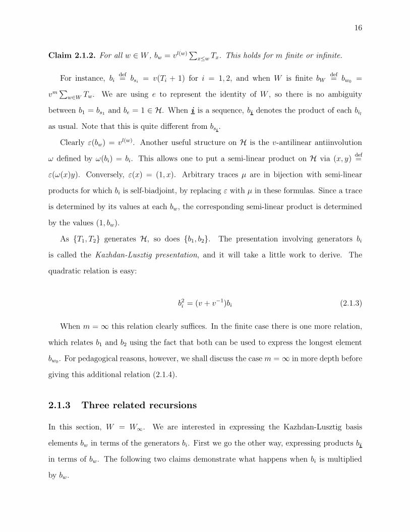
Claim 2.1.14. Any trace on the Hecke algebroid is determined by εe.

Proof. Because of the defining property of a trace, any endomorphism of any object which

can be expressed as a path going through e has its value determined by εe. The identity of

every object in H is given (up to a scalar) by a path through e, since we have the relation

BJeJ = [J ]bJ . Therefore, every path can be rewritten (up to a scalar) as a path through

e.

It is not hard to show that the standard trace on H extends to a trace on H, also called

the standard trace.

2.1.8 Induced trivial representations

Consider Hom(J, e) (resp. Hom(e, J)) for some J . This is none other than the left (resp.

right) ideal generated by bJ inside H, and the left (resp. right) action of End(e) on this space

by composition is precisely the action of H on the ideal. The Hecke algebra for has a trivial

representation T, a left H-module. It is free of rank 1 as a Z [v, v−1]-module, and bi acts by

multiplication by v + v−1. When m < ∞ the trivial representation can be embedded inside

the regular representation of H by looking at the left ideal of bW . For a finitary parabolic

subset J ⊂ I, we may induce the trivial representation of HJ up to H to get a representation

TJ , and this can also (less obviously) be embedded inside the regular representation of H

by looking at the left ideal of bJ . Therefore, this induced trivial module is none other than

Hom(J, e).

2.2 The Soergel categorification

2.2.1 The reflection representation

Let V = R2, equipped with the standard euclidean product. Choose two distinct lines in V

which form angle θ. We let q = eiθ. Define an action of W∞ on V by letting s be reflection

24

across the first line, and t be reflection across the second. The product st will be rotation

by 2θ, and the order of this rotation will determine which quotient Wm acts on V faithfully.

Let R be the polynomial ring of V , equipped with the induced action of W . The ring R

is graded, with linear functionals placed in degree 2. Choose two linear functionals fs and

ft, such that s(fs) = −fs and t(ft) = −ft (we also denote these f1 and f2, or fr and fb).

Clearly R ∼= R[fs, ft].

Let Ri denote the subring invariant under si. There is a map ∂i : R → Ri, known

as the Demazure operator or divided difference operator, where ∂i(f) = f−sif

fi. It is well-

defined since the numerator must divide the denominator, being si-anti-invariant. The map

is clearly Ri-linear, of degree −2, and ∂i(fi) = 2. Also, ∂i(f) = 0 if f ∈ Ri, and ∂i(fg) =

∂i(f)g + si(f)∂i(g).

Claim 2.2.1. There is an isomorphism of graded Ri-modules R ∼= Ri ⊕ Ri{2}.

Proof. The map from left to right is g 7→ (12∂i(gfi), ∂i(g)) and the map from right to left is

(g, h) 7→ g + 12fih. We leave the calculation to the reader.

In fact, we can say more: the ring R is actually a Frobenius extension of Ri. More details

are found in the next section.

The Cartan matrix is ai,jdef= ∂i(fj). As usual, ai,i = 2. Rescaling the generators fs and

ft may alter ai,j but not the product ξ = as,tat,s = 4 cos2(θ) = [2]2. Note that ξ = 4 is

impossible because θ 6= 0. We will not care about the action of W on V , but only on the

algebraic story, the action of W on R. As such, it is unnecessary to work over the base fieldR. We may work over any base ring k which contains the values ai,j. If 2 is not invertible,

we need to find another proof of Claim 2.2.1 (see section 2.2.4). Trigonometric identities

will transform into algebraic statements about the values of ai,j and ξ, which we discuss in

section 2.2.2. Henceforth, we will define everything algebraically, replacing as,t and at,s with

variables x and y respectively.

Definition 2.2.2. We let the universal ring be Ru = Z[x, y, (xy − 4)−1, fs, ft], graded with

25

fs, ft in degree 2 and x, y in degree 0. We place an action of the infinite dihedral group W∞

on Ru via s(fs) = −fs, s(ft) = ft − xfs, t(ft) = −ft and t(fs) = fs − yft. The W∞ action

on the degree 0 part is trivial. We define the subrings Riu and the Demazure operators as

before.

Notation 2.2.3. We let K denote the ring Z[x, y, (xy − 4)−1]. We will always use k to

represent a K-algebra to which we might want to specialize. We let Rk = Ru ⊗K k. We will

still denote the linear terms of Rk by V ∗. When it is irrelevant which k is chosen, or when

k is understood, we simply denote the ring by R.

We see that x = ∂s(ft) and y = ∂t(fs). Whenever we switch s and t, we should also

switch x and y. We write ξ = xy. Because x and y are algebraically independent in Ru, the

action of W∞ is faithful.

2.2.2 Trigonometry and Two-colored Quantum Numbers

We now investigate algebraically the condition that Rk admits an action of Wm for m < ∞.

The case when x = y = −[2] for some q should be familiar to anyone well-versed in quantum

numbers. In fact, what occurs below is a two-color variation on quantum numbers, appearing

in the two-colored Temperley-Lieb algebra.

Using the basis {fs, ft} for the degree 2 part of Ru, we see that the matrix of st is precisely

A =

xy − 1 x

−y −1

.

Definition 2.2.4. We define a family of polynomials Qk ∈ Z[ξ] inductively, for k ≥ 1. Start

with Q0 = 0 and Q1 = Q2 = 1. When k is odd, we let Qk = ξQk−1 −Qk−2. When k is even,

we let Qk = Qk−1 − Qk−2.

Example 2.2.5. Q3 = ξ − 1, Q4 = ξ − 2, Q5 = ξ2 − 3ξ + 1.

Claim 2.2.6. Consider the coefficients dqp from Definition 2.1.11. Then for k odd, Qk =

∑q∈c(k) dq

kξq−12 . For k even, Qk =

∑q∈c(k) dq

kξq−22 .

26

Claim 2.2.7. We have Ak =

Q2k+1(ξ) xQ2k(ξ)

−yQ2k(ξ) −Q2k−1(ξ)

.

Claim 2.2.8. The following are equivalent (even in characteristic 2):

• Q2m = 0 and Q2m−1 = −1

• Q2m−k = −Qk for 0 ≤ k ≤ 2m

• Qm = 0.

The proofs are simple exercises.

A specialization Rk admits an action of Wm for 2 ≤ m < ∞ if and only if Am is the

identity matrix, which is equivalent to Q2m+1 = 1, Q2m−1 = −1, and xQ2m = yQ2m = 0

(and one of the first two equations is redundant). Thus Z[x, y]/(xQ2m, yQ2m, Q2m−1 + 1) is

the universal ring admitting an action of Wm. We don’t really wish to work in this much

generality (although if you do, be my guest!). Let us make the further assumption that x, y

are either zero or non-zero-divisors, and the common assumption in Cartan matrices that

x = 0 ⇐⇒ y = 0. If x = y = 0 then A has order 2. Ignoring m = 2 we know that x, y 6= 0

so that Q2m = 0 is our replacement relation. By the above claim, Q2m = 0 and Q2m−1 = −1

is equivalent to Qm = 0.

Definition 2.2.9. We say that a Z[x, y]-algebra k is m-admissible if it factors through the

following quotient. When m = 2, we have x = y = 0. When 3 ≤ m < ∞, we have

Qm(xy) = 0.

Let us change our notation to place everything in a more familiar context.

Claim 2.2.10. Inside Z [q, q−1], we have Qk([2]2) = [k] when k is odd, and Qk([2]2) = [k][2]

when k is even.

The typical specialization is x = y = −[2], for which the matrix Ak =

[2k + 1] −[2k]

[2k] −[2k − 1]

.

(Whether one uses x = [2] or x = −[2], such as for the value of a circle in the Temperley-Lieb

27

algebra, is a matter of convention; we always use −[2].) Instead of specializing this way, we

merely use the symbol [k]x to denote Qk(xy) ∈ Z[x, y] when k is odd, and −xQk(xy) when

k is even. We use [k]y accordingly, and call these the two-colored quantum numbers. When

k is odd, [k]x = [k]y, and we may denote it by [k]x,y for emphasis. The two-colored quantum

numbers replace the usual quantum numbers when doing any computations with the two-

color Temperley-Lieb algebras (such as calculating coefficients of Jones-Wenzl projectors).

One should think of two-colored quantum numbers as though they were actual quantum

numbers.

Any identity involving quantum numbers has an analogous identity for two-colored quan-

tum numbers. For instance, [2]x[k]y = [k + 1]x + [k − 1]x.

Claim 2.2.11. When k divides m, Qk divides Qm in Z[ξ], and [k]x divides [m]x in Z[x, y].

Proof. Consider the remainder term when dividing Qm by Qk. This polynomial vanishes

when evaluated at any ξ = [2]2 ∈ R, and therefore is zero everywhere.

We are interested in a faithful action of Wm on R, not merely an action. We need Qm = 0

and Qk 6= 0 for any k < m. This can be established by looking at the analog of the cyclotomic

polynomials.

Definition 2.2.12. Let Pk be defined inductively by letting Pk = Qk/(∏

d|k Pd).

Note that the Pk, the analogs of cyclotomic polynomials, also have integer coefficients

(one can use the same arguments as for cyclotomic polynomials themselves). For complex

numbers, Pk(ξ) = 0 if and only if ξ = [2]2 where q2 = ζk.

Remark 2.2.13. For reasons which will become obvious in section 2.2.5, we also want to

assume that m is invertible.

Definition 2.2.14. Let Rm be the universal “nice” ring admitting a faithful action of Wm.

When m = 2, Rm = Z[x, y, 12]/(x, y). When m ≥ 3, Rm = Z[x, y, (xy−4)−1, m−1]/(Pm(xy)).

We say k is m-faithful if the specialization factors through Rm, and write it as km. Whenever

we say a ring is m-faithful we imply that m < ∞.

28

Remark 2.2.15. Sometimes Pm(xy) = 0 implies that xy − 4 is invertible, and sometimes it

does not. For instance, when m = 2, 4 we must invert 2, while for m = 3, 5, 6 we need not

invert anything. It never happens that Pm(xy) = 0 =⇒ xy − 4 = 0. Usually (or always?)

the conditions that Pm(xy) = 0 and xy − 4 is invertible imply that m is invertible.

Before we pass on to other matters, let us address one further specialization. In order

to have complete color symmetry, setting x = y is not enough. When m is odd, we must

also require the algebraic analog of the fact that q = ζ2m, not ζm. See section 2.3.3 for the

significance of this. This distinction is invisible in terms of algebraic conditions on ξ. Assume

that x = y below, and Pm(x2) = 0. For normal quantum numbers, [m + 1] = q−1[m] + qm so

that when [m] = 0, [m + 1] = qm = ±1. Therefore, ignoring q, our analogous condition will

be [m + 1]x = −1, or [m − 1]x = 1. This is already implied by Pm = 0 when m is even.

Definition 2.2.16. We say that an m-faithful ring k is m-symmetric if it factors through

x − y = 0 and xQm−1(x2) − 1 = 0, and if m is invertible.

Most of the results in this paper will be stated for m-symmetric rings, but could be

extended to work for m-faithful rings after some painful tweaking.

2.2.3 Invariant Subrings

Let L denote the set of L ∈ V ∗ (up to scalar) such that L = 0 cuts out a reflection line. Then

L = Ls∪Lt, where Ls = {fs, t(fs), st(fs), . . .} and Lt = {ft, s(ft), ts(ft), . . .}. When m = ∞

these two subsets are both infinite and disjoint. Over an m-faithful ring, both subsets are

finite, and we terminate them at the appropriate place to avoid redundancy. When m is

even the two sets are disjoint, and when m is odd the two sets are equal (with the ordering

flipped). In this finite case, we denote by L the product of all L ∈ L, a polynomial of degree

m (which, in the doubled grading on R, is in graded degree 2m). It is not hard to show that

s(L) = t(L) = −L.

Let L⊥ denote the set of L ∈ V ∗ (up to scalar) such that L = 0 cuts out a line “perpen-

29

dicular” to a reflection line. For instance, L is perpendicular to fs if s(L) = L, so that the

perpendicular line is Ls = xfs − 2ft. The perpendicular line to ft is Lt = yft − 2fs. One

can easily check that (for the right choice of scalars) L⊥ ⊂ Ru. Over an m-faithful ring, L⊥

is finite, and we denote by Z the product of all L ∈ L⊥, a polynomial of degree m. It is not

hard to show that s(Z) = t(Z) = Z.

There is also a polynomial z = xf 2s −xyfsft + yf 2

t of degree 2, for which s(z) = t(z) = z.

When x = y we may instead use z = f 2s + f 2

t − xfsft. Over an m-faithful ring, z and Z

generate all the W -invariants RWk

, and L generates the W -antiinvariants as a module over

RWk

. When W∞ acts faithfully, there are no antiinvariants, and the invariants are generated

by z.

We summarize. For any k, R = Rk, we have

Rs = k[f 2s , Ls] (2.2.1)

Rt = k[f 2t , Lt]. (2.2.2)

When x is invertible we may write

Rs = k[z, Ls] (2.2.3)

and similarly for y invertible and Rt.

When k is m-faithful we have

RW = k[z, Z]. (2.2.4)

When k is not m-faithful for any m < ∞ we have

RW∞ = k[z]. (2.2.5)

In particular, Ru and Riu are both rings of dimension 2 over K, while RW∞

u has dimension

1, so that the extension Riu ⊂ Ru is finite while the extension RW∞

u ⊂ Riu or Ru is infinite.

30

This is a general phenomenon related to whether or not the parabolic subgroup is finitary.

We only care about finite extensions of rings, so that we will never want to deal with RW∞

u .

R is a free module of rank 2 over Rs, generated by 1 and Lt. For instance, fs = yLs+2Lt

xy−4.

Moreover, ∂s(Lt) = xy−4 is invertible. Therefore, R is generated by 1 as a Rs −Rt-module,

and there is an element of Rt which maps by ∂s to 1.

2.2.4 Frobenius Extensions and Ri

Definition 2.2.17. Let A ⊂ B is an extension of commutative rings such that B is free and

finitely generated as an A-module, equipped with an A-linear map ∂ = ∂BA : B → A. We say

that two bases {aα} and {bα} for B over A are dual bases if ∂(aαbβ) = δαβ . If dual bases

exist, B is called a Frobenius extension of A.

For a Frobenius extension, one is equipped with a comultiplication map B → B ⊗A B,

which sends 1 7→ ∆BA =

∑α aα ⊗ bα for some dual basis. This element of B ⊗A B did

not depend on the choice of dual basis, and neither does µBA = µ(∆B

A) =∑

α aαbα ∈ A.

Frobenius extensions appear often in geometric representation theory, and are useful because

the functors of induction and restriction between A-mod and B-mod are biadjoint.

We will prove that, under certain circumstances, the invariant subrings will form a square

of Frobenius extensions, in the sense of [9]. In the notation ∆BA or ∂B

A we replace A and B by

either W, s, t or emptiness, as in ∂sW and ∆i. The smaller ring is always placed on bottom.

We have already defined ∂i. We will also use Sweedler notation for coproducts, so that

µs = ∆s(1)∆s(2).

The proof of Claim 2.2.1 relied on the presence of 12∈ R. In fact, it only relied on the

fact that ∂s(fs

2) = 1, but any other element f with ∂s(f) = 1 would work, such as Lt

xy−4.

Claim 2.2.18. Let f ∈ V ∗ for which ∂i(f) = 1. Then {1, f} forms a basis for R as a

free Ri-module, and {−s(f), 1} forms a dual basis over the map ∂i. Moreover, any pair of

dual bases can be formed as above by choosing such an f , up to multiplication by invertible

scalars. Therefore, Ri ⊂ R is a Frobenius extension, R ∼= Ri ⊕ Ri{2}, and µi = fi.

31

Proof. That {1, f} and {−s(f), 1} are dual is clear. The isomorphism R ∼= Ri ⊕ Ri{2} is

given by sending g ∈ R to (∂i(gf), ∂i(g)), and conversely by sending (g, h) 7→ g − s(f)h. We

leave the rest to the reader.

Here is an obvious corollary.

Claim 2.2.19. Letting Bidef= R⊗Ri R{−1}, we have an isomorphism of graded R-bimodules

Bi ⊗ Bi∼= Bi{1} ⊕ Bi{−1}. (2.2.6)

Proof. This is clear from the Ri-bimodule isomorphism R ∼= Ri⊕Ri{2}. Explicitly, choosing

f with ∂i(f) = 1, the map from left to right sends 1 ⊗ g ⊗ 1 7→ (∂i(fg) ⊗ 1, ∂i(g) ⊗ 1) and

the map from right to left sends (1⊗ 1, 0) 7→ 1⊗−1⊗ 1 and (0, 1⊗ 1) 7→ 1⊗−s(f)⊗ 1.

Equation (2.2.6) is a categorification of relation (2.1.3), as shall be seen.

Note that we may choose a pair of dual bases of R over Rs such that one bases lies within

Rt, and vice versa. This is a technical statement, used in [9].

2.2.5 Frobenius Extensions and RW

Now we wish to discuss the extensions RW ⊂ Ri and RW ⊂ R, which are only finite

extensions when W = Wm is a finite dihedral group. We assume for the rest of the chapter

that k is m-symmetric for some m ≥ 2. There is a more general Demazure operator ∂W : R →

RW , whose degree is −2m. It is defined by letting i be a reduced expression for w0, and

letting ∂W = ∂idef= ∂i1∂i2 . . . ∂im . This does not depend on the choice of reduced expression

if k is m-symmetric. There are also relative Demazure operators ∂iW : Ri → RW , defined by

letting i be a relative reduced expression for w0. For example, ∂sW = ∂t∂s∂t · · ·∂t︸ ︷︷ ︸

m−1

, because

tst · · · t is a reduced expression for w0 after multiplying by s. These Demazure operators

make each inclusion a Frobenius extension.

32

These definitions imply that ∂sW ∂s = ∂t

W ∂t, which states that this square of Frobenius

extensions is compatible, in the sense of [9]. It is possible but annoying to alter the results

for the m-faithful case, where the Frobenius square is only compatible up to a scalar. One

must keep track of this scalar everywhere below (and even in isotopy of diagrams, see [9]),

which we have not done.

Theorem 1. Suppose that k is m-symmetric. Then the extensions RW ⊂ R and RW ⊂ Ri

are Frobenius extensions. Therefore, R is a free RW -module of graded rank [W ], and Ri is a

free RW -module of graded rank [W ](v+v−1)

. Any dual bases satisfy the following properties. The

latter ones involve considering an element of Rs as though it were in R and taking ∂t of it.

µW = L (2.2.7)

µsW =

L

fs

(2.2.8)

∆sW (1)∂t(∆

sW (2)) = ∂t(∆

sW (1))∆

sW (2) =

L

fsft

(2.2.9)

∆sW (1) ⊗ ∂t(f∆s

W (2)) = ∂s(f∆tW (1)) ⊗ ∆t

W (2) ∈ Rs ⊗RW Rt for any f ∈ R (2.2.10)

In particular, the map R → Rs⊗RW Rt sending f 7→ ∆sW (1)⊗∂t(f∆s

W (2)) = ∂s(f∆tW (1))⊗

∆tW (2) is well-defined, Rs-linear on the left, and Rt-linear on the right.

Sketch of Proof. First, we need to show that Rs is a Frobenius extension of RW . One need

only find dual bases. Computing these bases explicitly is a calculation, but showing that

dual bases exist is not difficult via a constructive argument. Once one chooses a basis (say,

powers of Ls) then one need only find a dual basis, which one can show exists inductively.

The tricky part is that the coefficients in these bases lie within km. Essentially, however,

this will follow from the fact that m is invertible, that L

fs∈ Rs, and that ∂s

W ( L

fS) = m. This

can be checked by hand.

The equations above hold in general for any square of Frobenius extensions, as shown in

[9]. The only interesting piece of data is that µW = L. This even implies that ∂sW ( L

fS) = m,

33

since for any Frobenius extension, ∂BA (µB

A) is equal to the degree of B over A. To show that

µW = L, note first that ∂s(µW ) = ∂s(µsWµs) = 2µs

W = 2µW

fs. By the definition of ∂s, we see

that s(µW ) = −µW . Also, t(µW ) = −µW . So µW is antiinvariant, and for degree reasons

must be equal to L.

Corollary 2.2.20. Letting BWdef= R ⊗RW R{−m} we have the following isomorphisms:

Bi ⊗ BW∼= BW ⊗ Bi

∼= (v + v−1)BW (2.2.11)

BW ⊗ BW∼= [W ] BW (2.2.12)

We mention briefly that, choosing any basis {aα} with dual basis {bα} that the [W ]-many

projection maps from R to RW are f 7→ ∂W (faα) and the inclusion maps are g 7→ gbα. These

maps, applied to the middle factor in R⊗RW R⊗RW R, give you the projections and inclusions

in (2.2.12) as well. To deduce (2.2.11) we write R ⊗Ri R ⊗RW R as R ⊗Ri R ⊗Ri Ri ⊗RW R

and reduce the second factor of R as in Claim 2.2.18.

2.2.6 Soergel Bimodules

Definition 2.2.21. As in the introduction, let BBS denote the subcategory of R-modules

generated (over ⊗, ⊕, {1}) by Bs and Bt, and let B denote its Karoubi envelope. When

R = Rm, let BgBS denote the subcategory generated by Bs, Bt, and BW . When R = Ru we

write BBS,u and Bu. When k = km is m-faithful, we may write Bm instead of Bk.

Remark 2.2.22. We will show that, under suitable conditions on km, the bimodule BW is

a summand of Bs ⊗ Bt ⊗ Bs ⊗ · · ·︸ ︷︷ ︸m

, so that it lives inside Bm already, and Bm is also the

Karoubi envelope of BgBS,m.

Remark 2.2.23. The category BBS,k is not simply the base change of the category BBS,u. The

modules have had their base changed, but in the new ring there may be additional morphisms

which were not present before, and the graded rank of the Hom spaces may change. In fact,

34

we will show that the new morphisms in Bm that are not in Bu are generated by a single

new morphism of degree 0.

Theorem 2. (See Soergel [27] Theorems 1.10, 4.2, 5.5, 6.16) Let m ≥ 2 or m = ∞. Let

k be an infinite field of characteristic 6= 2, and let W = Wm be the dihedral group acting

faithfully on R = Rk. There is a map from H to the Grothendieck ring of B sending v to

[R{1}], bi to [Bi], and bW to [BW ] when m < ∞. This map is an isomorphism. There is one

indecomposable bimodule Bw ∈ B for each w ∈ W , and if i is a sequence giving a reduced

expression of w then Bw is a summand of Bi of multiplicity 1. For dihedral groups, we know

that this isomorphism also sends bw to [Bw]. For two objects X, Y ∈ B, the space Hom(X, Y )

is a free left (or right) R-module of graded rank ([X], [Y ])def= ε(ω([X])[Y ]).

Remark 2.2.24. Soergel’s results apply in great generality to other Coxeter groups. In the

general case, one can still say that the indecomposables Bw are in bijection with W , but can

not assert that they descend to the Kazhdan-Lusztig basis.

Remark 2.2.25. We believe that Soergel’s techniques could have been generalized to other

base rings, although it is somewhat subtle. We present a different method towards proving

these results for dihedral groups over more general rings k. We will call k a Soergel ring

when we want to emphasize that the full force of Soergel’s results may be brought to bear.

For now, this just means an infinite field of characteristic 6= 2.

2.2.7 Singular Soergel Bimodules

Definition 2.2.26. Let Bim denote the 2-category whose objects are rings, and for which

Hom(B, A) is the category of A − B-bimodules. Let BBS denote the full (additive, graded)

sub-2-category whose objects are RJ for J finitary, and whose 1-morphisms are generated

by RJ as an RJ − RK-bimodule and as a RK − RJ -bimodule, whenever J ⊂ K. These

are known as induction and restriction bimodules, respectively. Its Karoubi envelope is the

2-category of singular Soergel bimodules, denoted B. As usual, we use the subscript u when

35

this is done over R = Ru, the subscript k for R = Rk, and the subscript m when R = Rm.

Theorem 3. (See Williamson [31] Theorems 7.5.1, 7.4.1 and others) Let k be a Soergel

ring. There is a functor from H to the Grothendieck category of B, sending v to the grading

shift and bJ ∈ Hom(J, K) to RJ ∈ Hom(RJ , RK) for J ⊂ K, and similarly for Hom(K, J).

This map is an isomorphism, and over the empty parabolic it restricts to the isomorphism

from H to [B]. There is a formula for calculating the size of 2-morphism spaces in B by

using the standard trace map on H.

2.3 Temperley-Lieb categories

2.3.1 The Uncolored Temperley-Lieb category

The (uncolored) Temperley-Lieb algebra on n strands TLn is an algebra over Z[d] which

can be realized pictorially. It has a basis given by crossingless matchings with n points on

bottom and n on top (see the example below). Multiplication is given by concatenation of

diagrams, and by replacing any closed component (i.e. circle) with the scalar d. We denote

the crossingless matching representing the identity element by 1n.

Example 2.3.1. An element of TL10:

The Temperley-Lieb algebra is part of the Temperley-Lieb category T L, a monoidal

category whose objects are n ∈ N, thought of as n points on a line, and where the morphisms

from n to m are spanned by crossingless matchings with n points on bottom and m on top.

Composition is given by concatenation and resolving circles, as usual, so that End(n) = TLn.

As a monoidal category we should really view it as a 2-category with a single object, the

uncolored region.

Let U = Uq(sl2) be the quantum group of sl2. Let Vk be the irreducible representation

with highest weight −qk, and let V = V1. We have already remarked that the Temperley-Lieb

category governs the intertwiners between tensor products of V , so that HomT L(n, m) ⊗Z[d]

36Q(q) = HomU(V ⊗n, V ⊗m). Under this base change, d 7→ −[2], and we use quantum numbers

interchangeably with the polynomials in d that express them.

Proposition 2.3.2. The Temperley-Lieb algebra TLn, after extension of scalars, contains

canonical idempotents which project V ⊗n to each isotypic component. It contains primitive

idempotents refining the isotypic idempotents, which project to each individual irreducible

component (although this splitting is non-canonical). Given a choice of primitive idempo-

tents, TLn contains maps which realize the isomorphisms between the different irreducible

summands of the same isotypic component. These maps can be defined in any extension ofZ[d] where the quantum numbers [2], [3], . . . , [n] are invertible.

Proof. The only part of this proposition which is not tautological is the statement about

coefficients. This follows from recursion formulas for the idempotents, some of which can be

found below. For more on recursion formulas and coefficients see [10].

We say an extension of Z[d] is TLn-sufficient if the first n quantum numbers are invertible,

and is TL-sufficient if it is TLn-sufficient for all n.

The highest non-zero projection, from V ⊗n to Vn, is known as the Jones-Wenzl projector

JWn ∈ TLn. Here are some examples of Jones-Wenzl projectors.

Example 2.3.3.

+

+ +

+ +

= =

=

JW1 JW2

JW3

1[2]

1[3]

1[3]

[2][3]

[2][3]

Claim 2.3.4. Jones-Wenzl projectors satisfy the following relevant properties:

• JWn is the unique map which is killed when any cap is applied on top or any cup on

bottom, and for which the coefficient of 1n is 1.

• The ideal generated by JWn in TLn is one-dimensional over Q(d), since any other

element x ∈ TLn acts on JWn by the coefficient of 1n in x.

37

• JWn is invariant under left-right and top-bottom reflection.

• The coefficient of every crossingless matching in JWn is non-zero.

• JWn can be defined so long as [n] is invertible.

• There is a recursive formula (see [30]) which is:

=...

...

...

...+

...

...

...

...JWn

JWn

JWnJWn−1JWn+1

[n][n+1]

. (2.3.1)

It is more typical to see this formula with JWn−1 replaced by 1n−1.

• There is an alternate recursive formula ([10], Theorem 3.5), which sums over the

possible positions of cups, and follows quickly from (2.3.1):

=...

...

...

...+

n∑

a=1

JWnJWnJWn+1

[a][n+1]

a

. (2.3.2)

In Kar(T L) we let Vn denote the image of JWn and (·)⊗V denote the functor of adding

a new line on the right. The recursive formula (2.3.1) gives a diagrammatic proof of the

following obvious proposition.

Proposition 2.3.5. The Karoubi envelope Kar(T L) of T L has indecomposables Vn, n ∈ N.

These satisfy V ⊗ V0∼= V0 ⊗ V ∼= V1 and V ⊗ Vn

∼= Vn ⊗ V ∼= Vn+1 ⊕ Vn−1 for n ≥ 1.

The proofs of the above facts are standard. Some references on the Temperley-Lieb

algebra and planar algebras include [11, 3, 10, 21]. In particular, formulae for Jones-Wenzl

projectors were produced in [10]; the unpublished paper [21] has a more detailed version.

38

Let us pause to calculate the coefficient ρk of in JWk, using (2.3.2). The first

term on the right hand side contributes nothing to this coefficient. The sum only contributes

when a = 1, and it contributes [1][k]

times the coefficient of 1k−2 in JWk−2, which is 1. Therefore

ρk = 1[k]

. When q = ζ2(k+1), [k] = 1 and ρk = 1.

2.3.2 The Two-colored Temperley-Lieb Category

Any 1-manifold will divide the plane into regions which can be colored alternately with 2

colors. Let us assume these two colors are red and blue. We may construct a variation on the

Temperley-Lieb algebra by coloring the regions, and specifying different values for a circle

based on its interior color. The two-color Temperley-Lieb 2-category 2T L has two objects,

red and blue, and its 1-morphisms are generated by a point on a line either switching blue to

red or vice versa. The 2-morphisms are the Z[x, y]-module spanned by appropriately-colored

crossingless matchings. Multiplication is defined as in T L except that a circle with red (resp.

blue) interior evaluates to x (resp. y).

Example 2.3.6. An element of Hom(rbrbrb, rbrb):

Note that there is no 1-morphisms from red to red, or from blue to blue, so that the

colors must alternate. A 1-morphism (and its source and target objects) can be specified

by the alternating sequence of colors it passes through (e.g. rbrbrb). Fixing a number of

strands and a color (say, the rightmost color), we get an algebra which we might call the

two-color Temperley-Lieb algebra 2TLn.

Example 2.3.7. An element of 2TL10:

If we specialize to x = y = d, we may forget the colors and obtain the usual uncolored

Temperley-Lieb category. The difference between TL and 2TL is not very large, consisting

of a minor generalization of coefficients. However, adding colors does restrict which 1-

morphisms and 2-morphisms can be concatenated. In 2T L there are 4 kinds of diagrams

(depending on whether blue or red appears on the left and right), corresponding to the 4

39

Hom categories between the 2 objects. In other words, a 2-morphism which has blue on the

right and red on the left in the source also has blue on the right and red on the left in the

target.

Jones-Wenzl projectors JWn exist in 2T L as well, one for each number of strands and

choice of rightmost color. Its coefficients will involve inverting two-colored quantum numbers

[n]x and [n]y. The recursion formulae (2.3.1) and (2.3.2) can be generalized, using two-color

quantum numbers. We give examples of the first few projectors, when blue is the rightmost

color.

Example 2.3.8.

−

− −

+ +

= =

=

JW1 JW2

JW3

1x

1xy−1

1xy−1

xxy−1

yxy−1

As mentioned in the introduction, people tend to use the spherical or lopsided special-

ization of 2T L, so that the references for the facts below may be more difficult to find. The

proofs, however, are completely analogous to the uncolored case.

Proposition 2.3.9. The canonical isotypic idempotents, the non-canonical primitive idem-

potents, and the intra-isotypic isomorphisms of Proposition 2.3.2 all have analogs in 2TLn

after localization. More precisely, there are two versions of each idempotent, one with red on

the right and one with blue. These maps are defined over any extension of Z[x, y] for which

the two-color quantum numbers up to [n] are invertible.

We say that a specialization k of Z[x, y] is 2TLn-sufficient if primitive idempotents and

intra-isotypic isomorphisms can be constructed in 2TLn using coefficients in k. We say it is

2TL-sufficient if it is 2TLn-sufficient for all n.

Every indecomposable in the Karoubi envelope of T L is doubled in the Karoubi envelope

of 2T L because of the two choices of color. For instance, V0 is replaced by two distinct

40

indecomposables, Vb and Vr, represented by the empty diagram with the region colored blue

or red respectively. Similarly, V1 is replaced by Vrb and Vbr, and so forth.

Proposition 2.3.10. The Karoubi envelope Kar(2T L) of 2T Lk (for a 2TL-sufficient ring

k) has indecomposables Vi where i is an nonempty alternating sequence of red and blue.

Therefore, there are two sequences of each length n ≥ 1. We denote by r ⊗ · the functor

of placing a line on the left with the lefthand region colored red; this operation can only be

performed on a 1-morphism which currently has blue in the lefthand region. This satisfies

r ⊗ Vb∼= Vrb and r ⊗ Vbr...

∼= Vrbr... ⊕ Vr... for any appropriate sequence i = br . . . of length

≥ 2. Similar statements are made switching r and b, or switching left and right.

Note that we can label these indecomposables by the elements of W∞ \ {e}. The multi-

plication rule given here is a categorification of the rule given in Claim 2.1.4.

2.3.3 Roots of Unity and Rotation

It is well known that when [m] = 0, the Jones-Wenzl projector JWm−1 ∈ TLm−1 is negligible.

This is equivalent, for Jones-Wenzl projectors, to the statement that

...

...= 0JWm−1 .

In fact, JWm−1 is negligible (when it is defined) if and only if [m] = 0. See [11] for more

details.

In particular, rotating JWm−1 by any number of strands yields another morphism which

is killed on the top and bottom by all cups and caps, and is therefore a scalar multiple

of JWm−1. We say that JWm−1 has a “rotational eigenvalue.” Conversely, if JWm−1 has

a rotational eigenvalue, then it must be negligible. To compute this eigenvalue one may

compare the coefficients of two pictures which are related by rotation. Rotation by 2 strands

always has eigenvalue 1, since the following picture is unchanged after rotation by 2 strands.

or

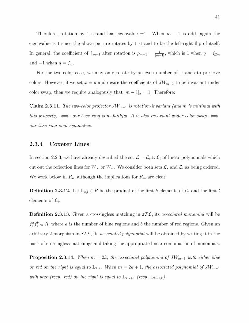
41

Therefore, rotation by 1 strand has eigenvalue ±1. When m − 1 is odd, again the

eigenvalue is 1 since the above picture rotates by 1 strand to be the left-right flip of itself.

In general, the coefficient of 1m−1 after rotation is ρm−1 = 1[m−1]

, which is 1 when q = ζ2m

and −1 when q = ζm.

For the two-color case, we may only rotate by an even number of strands to preserve

colors. However, if we set x = y and desire the coefficients of JWm−1 to be invariant under

color swap, then we require analogously that [m − 1]x = 1. Therefore:

Claim 2.3.11. The two-color projector JWm−1 is rotation-invariant (and m is minimal with

this property) ⇐⇒ our base ring is m-faithful. It is also invariant under color swap ⇐⇒

our base ring is m-symmetric.

2.3.4 Coxeter Lines

In section 2.2.3, we have already described the set L = Ls ∪ Lt of linear polynomials which

cut out the reflection lines for W∞ or Wm. We consider both sets Ls and Lt as being ordered.

We work below in Ru, although the implications for Rm are clear.

Definition 2.3.12. Let Lk,l ∈ R be the product of the first k elements of Ls and the first l

elements of Lt.

Definition 2.3.13. Given a crossingless matching in 2T L, its associated monomial will be

fas f b

t ∈ R, where a is the number of blue regions and b the number of red regions. Given an

arbitrary 2-morphism in 2T L, its associated polynomial will be obtained by writing it in the

basis of crossingless matchings and taking the appropriate linear combination of monomials.

Proposition 2.3.14. When m = 2k, the associated polynomial of JWm−1 with either blue

or red on the right is equal to Lk,k. When m = 2k + 1, the associated polynomial of JWm−1

with blue (resp. red) on the right is equal to Lk,k+1 (resp. Lk+1,k).

42

Remark 2.3.15. Note that, in either case, the polynomial in question will descend to L in Rm

(up to a scalar). Therefore, this polynomial cuts out in h the union of all the reflection-fixed

lines.

This proposition is the analog of Section 3.7 in [6]. In that paper we examine Soergel

bimodules in general type A, not in dihedral type, and instead of a single polynomial we

obtain an ideal in k[f1, f2, . . . , fn]. This ideal cuts out the Coxeter lines in hsln (there

called the “Weyl lines”), which are the lines given by transverse intersections of reflection

hyperplanes in h. While it is not obvious in this dihedral setup for reasons of dimension,

what we are doing is creating an ideal which cuts out lines, not one that cuts out codimension

one reflection hyperplanes.

Proof. We prove this statement inductively. Let Ym,b denote the associated polynomial of

JWm with blue on the right. Let L denote the k + 1-st line in Lt. We will be done if we can

show that Ym+1,b = LYm,r for either m = 2k or m = 2k +1, and the same for the color swap.

We need the 2-colored version of (2.3.2). The differences between the one-colored and

two-colored versions are

1. If n + 1 is even, then [n + 1] becomes [n + 1]x,y.

2. If n+1 is odd, then the outsides are the same color. If this color is blue, [n+1] becomes

[n + 1]x, and otherwise becomes [n + 1]y.

3. In the sum, [a] becomes [a]x if the interior of the new cup is blue, and [a]y if the interior

is red.

The recursive formula says that Ym+1,b = 1[m+1]x

Ym,r(∑m+1

a=1,n+1−a even [a]yft+∑m+1

a=1,n+1−a odd [a]xfs).

The term a = n + 1 comes from the first term of (2.3.2). Thus it is enough to show that

(∑m+1

a=1,n+1−a even [a]yft +∑m+1

a=1,n+1−a odd [a]xfs) is an expression for L (up to a scalar). This,

too, can be proven by induction, dealing with the cases of even and odd separately. We leave

this exercise to the intrepid reader.

43

Remark 2.3.16. Every coefficient in JWm is nonzero. There is only a single crossingless

matching with precisely one blue (resp. red) connected component, giving a nonzero leading

term cfsfmt . Therefore the associated polynomial of JWm is nonzero when k is 2TLm-

sufficient.

2.4 Main Techniques

2.4.1 Diagrammatics and Rotation

There are numerous excellent introductions to diagrammatics for cyclic (i.e. pivotal) monoidal

categories and 2-categories, such as chapter 4 of [19]. For an example of a diagrammatic

category which is self-biadjoint, see [7].

We make only one remark, also made in [7]. Cyclicity states that taking any mor-

phism and using adjunction maps to rotate it by 360 degrees will not change the morphism.

Cyclicity is required to draw morphisms on a plane, because any symbol we use to depict the

morphism is evidently invariant under 360 degree rotation. However, consider a morphism

with boundary Bs⊗Bs⊗Bs, reading around the circle. It is possible to rotate this morphism

by 120 degrees, and cyclicity is no guarantee that this will not change the morphism. If it

is the case that 120 degree rotation does not change the morphism, then one may depict

the morphism using a diagram which is 120 degree rotation invariant, such as a trivalent

vertex. One may pose the same question for any 2-morphism whose boundary 1-morphism

has rotational symmetry. In this paper, we will also have morphisms whose boundary is

Bs ⊗ Bt ⊗ · · ·︸ ︷︷ ︸2m

, and it will be invariant under rotation by 360m

degrees, so that we may draw

it as a two-colored 2m-valent vertex (see section 4.1).

When one gives a diagrammatic category by generators and relations, and generators are

drawn to have some non-trivial rotational invariance, then there is a hidden relation (called

the isotopy relation) which states that rotating that 2-morphism does nothing. This relation

will go unstated, but will need to be checked when applying functors into non-diagrammatic

44

categories.

2.4.2 Hom spaces and Grothendieck rings

Suppose that C is a k-linear graded additive monoidal category with objects Bi for i =

1, 2, satisfying relation (2.2.6). Let B∅ denote the monoidal identity. There is an obviousZ [v, v−1]-linear map from H∞ to the Grothendieck ring [C], sending bi 7→ [Bi]. If in addition

C satisfies the categorified version of (2.1.4) for some m < ∞, then this map factors through

the finite Hecke algebra Hm. We need not assume the existence of an object which categorifies

bw0 , only that tensor products of Bi satisfy this isomorphism. If C satisfies the Krull-Schmidt

property, one can deduce that such an object Bw0 does exist; we will not use this fact, and

leave the proof to the reader. Let W be the Coxeter group acting faithfully and H its Hecke

algebra.

The category C induces a semi-linear pairing on H, via (bi , bj ) 7→ grkkHomC(Bi , Bj ). If, in

addition, each object Bi is self-biadjoint, then biadjointness descends to the map ω : H → H,

and the semi-linear pairing is determined by the map ε(bi ) = grkHom(B∅, Bi). We use the

graded rank, which is well-defined even though we do not assume that Hom spaces are free.

Lemma 2.4.1. Let C be a category as above (with Bi self-biadjoint), and let ε be any trace

map on H. Suppose that

• For each w ∈ W there is an object Bw for which bw 7→ [Bw]. The biadjoint of Bw is

Bw−1.

• The categorified version of the relation in Claim 2.1.9 holds, decomposing Bi for a

reduced expression i into direct sums of Bw.

• The Hom spaces HomC(B∅, Bw) are free k-modules for all w ∈ W . (More generally,

we may assume they are free R-modules for some k-algebra R for which composition

in C is R-linear.)

45

• The graded rank of HomC(B∅, Bw) over k (resp. over R) is equal to ε(bw).

Then we may deduce that

• All Hom spaces between various objects Bw and Bi in C are free as k-modules (resp.

as R-modules).

• For any sequences i, j we know that HomC(Bi, Bj) has graded rank over k (resp. R)

equal to (bi, bj), the semi-linear product induced by ε. The same is true replacing i or

j with w for any w ∈ W .

Proof. We note first that we may replace the category C with its subcategory consisting

of direct sums of summands of various Bw. This is the Karoubi envelope of the monoidal

category generated by B1 and B2, and it is itself closed under monoidal product.

Using biadjointness and direct sum decompositions, we see that any Hom space between

various Bi or Bw is isomorphic to a direct sum of Hom spaces Hom(B∅, Bw) for various

Bw. Therefore the freeness of Hom(B∅, Bw) implies the freeness of all Hom spaces. The

combinatorics of biadjointness and decomposition in C are the same as the combinatorics of

ω and the additive relations in H when determining (x, y), so that the final statements are

obvious.

Corollary 2.4.2. Suppose that C satisfies the conditions of Lemma 2.4.1 for the standard

trace ε, as the graded rank of Hom spaces over a graded ring R. We assume that R is con-

centrated in non-negative degree, and has no nontrivial idempotents. Suppose that C consists

only of direct sums of summands of various Bi. Then each object Bw is indecomposable and

the category has the Krull-Schmidt property. The objects {Bw} for w ∈ W form a complete

list of non-isomorphic indecomposables up to grading shift. The map H → Kar[C] is an

isomorphism.

Proof. Calculations with the bilinear form imply that the graded rank of HomC(Bw, Bx) is

either in 1 + vZ[v] for w = x, or in vZ[v] for w 6= x. This is sufficient to imply that {Bw}

46

form a list of pairwise non-isomorphic indecomposables. Since every Bi splits into these

indecomposables, our list must be complete.

This observation was made by Soergel in [27] and elsewhere; that one need only show the

existence of objects Bw descending to bw to show that B categorifies the Kazhdan-Lusztig

basis, because once one has those objects abstract nonsense implies that they form a complete

list of non-isomorphic indecomposables.

Corollary 2.4.3. Suppose that C and D are two such categories as in Lemma 2.4.1. Assume

that C is generated by direct sums of summands of Bi, and that both categories have the Krull-

Schmidt property. Suppose F : C → D is an additive R-linear monoidal functor sending Bi

to Bi (which implies that Bw is sent to Bw). Suppose that F induces isomorphisms of Hom

spaces Hom(B∅, Bw) for all w, or alternatively of Hom(B∅, Bi) for every reduced expression

i. Then F is fully faithful.

Proof. Left to the reader.

The upshot of these statements is that one need only investigate very few Hom spaces to

understand or identify the entire category.

To see these proofs done in more detail for a completely analogous case, see section 3.3

of [6].

47

Chapter 3

Dihedral Diagrammatics: m = ∞

In this chapter we give a presentation of an Ru-linear diagrammatic category D(∞), and a

functor F : D(∞) → Bu. This functor will be an equivalence of categories after base change.

We will show, for sufficiently nice rings k over Z[x, y], that the category after base change

D(∞)k is a categorification of the Hecke algebra. In the Karoubi envelope Kar(D(∞)k), the

isomorphism classes of indecomposable objects are in bijection with the elements of W∞, so

we may label them Bw for w ∈ W∞. There is an isomorphism H∞ → [Kar(D(∞)k)] for

which bw 7→ [Bw].

The key to the proof is the observation that certain morphism spaces in D(∞) can be

described by the two-colored (type A) Temperley-Lieb category. In fact, the idempotents in

D(∞) which correspond to the indecomposable objects Bw (for w 6= e) are given by Jones-

Wenzl projectors. The theory of modules over the Temperley-Lieb algebra will provide us

with the information we need to check all the desired direct sum decompositions.

Once we have the existence of objects Bw, we will use Lemma 2.4.1 and its corollaries to

finish the proof. In order to do this, we need to investigate certain specific Hom spaces. To

show that these Hom spaces are not “too big” we use diagrammatic arguments to reduce all

pictures to certain forms. To show that they are not “too small” we evaluate the pictures

using the functor F to bimodules, and use this to demonstrate linear independence. Putting

48

this together, we pinpoint exactly the size of Hom spaces, and show that F is an equivalence.

In previous papers, we proved that H → [Kar(D)] was an isomorphism by constructing

an isomorphism D → B and using Soergel’s results, while here we prove it directly using

Corollary 2.4.2.

3.1 The category D(∞)

3.1.1 Definitions

Definition 3.1.1. A Soergel graph for m = ∞ is an isotopy class of a particular kind of

graph with boundary, properly embedded in the planar strip (so that the boundary of the

graph is always embedded in the boundary of the strip). The edges in this graph are colored

by either s or t. The vertices in this graph are either univalent (dots) or trivalent, with all

three adjoining edges having the same color. The boundary of the graph gives two sequences

of colors, the top and bottom boundary. Soergel graphs have a degree, where trivalent vertices

have degree −1 and dots have degree 1.

When there is no ambiguity we refer to a Soergel graph merely as a “graph,” even though

it is an isotopy class of embedded graph.

Definition 3.1.2. Let D(∞) be the Z[x, y, (xy − 4)−1]-linear monoidal category defined

herein. The objects will be finite sequences i = i1i2 . . . id of indices s and t, with a monoidal

structure given by concatenation. The space HomD(∞)(i , j ) will be the free Z[x, y, (xy−4)−1]-

module generated by Soergel graphs with bottom boundary i and top boundary j , modulo

the relations below. Hom spaces will be graded by the degree of the Soergel graphs.

In giving relations, we will always use the convention that blue represents s and red t.

The first four relations hold for both red and blue:

=(3.1.1)

49

= =(3.1.2)

= 0 (3.1.3)

+ = 2 (3.1.4)

The remaining relations, along with (3.1.4) above, are called forcing relations. They are:

= +− xx (3.1.5)

= +− yy (3.1.6)

The forcing relations immediately imply the sliding relations:

=−2 −2 xx (3.1.7)

=−2 −2 yy (3.1.8)

Remark 3.1.3. Technically, we have defined a non-graded, non-additive category whose Hom

spaces are enriched in graded k-modules. One can take its graded additive closure, which

formally adds direct sums and grading shifts, and restricts to degree 0 maps. This is a graded

additive category with exactly the same information. We always assume we are working with

the graded additive closure.

Definition 3.1.4. Let F = F∞ be the Z[x, y, (xy−4)−1]-linear monoidal functor from D(∞)

to BBS,u defined as follows. The object i is sent to Bi . A dot colored i can be oriented as

a map from i to ∅, or as a map from ∅ to i. The former is sent by F to the multiplication

map from R ⊗Ri R → R. The latter sends 1 ∈ R to ∆i ∈ R ⊗Ri R (see section 2.2.4). The

trivalent vertex colored i can be oriented as a map from ii to i or vice versa. The former is

sent by F to the map f ⊗ g⊗h 7→ f∂i(g)⊗h from R⊗Ri R⊗Ri R → R⊗Ri R, and the latter

50

is sent to the map f ⊗ g 7→ f ⊗ 1 ⊗ g in the opposite direction.

Claim 3.1.5. The previous definition gives a well-defined functor.

Proof. Not only must we show that the relations on D(∞) given above are satisfied by their

images in B, but we must show that the morphism designated by a graph is independent of

the graph’s embedding into the plane. This latter statement corresponds to some additional

“isotopy relations,” as pictured here.

==(3.1.9)

= = (3.1.10)

For the first four relations and the isotopy relations, this was proven in [7], and we leave

the simple computation to the reader. We will discuss the sliding and forcing relations

presently.

3.1.2 Double Dots

Under the functor F , a double dot colored i (such as those appearing in the forcing and

sliding relations) will be sent to the polynomial µi = fi ∈ Ru. Placing double dots in the

leftmost and rightmost regions will yield an Ru-bimodule structure on Hom spaces.

One should think of the vertical line colored i as being the identity map of Bi. The

bimodule Bi is designed so that left and right multiplication are the same for polynomials

invariant in si. The sliding relations say precisely that Ls = 2ft − xfs slides through a blue

line, and Lt slides through a red line. Using (3.1.4) one can show that f 2s slides through a

blue line as well. Since Ls and f 2s generate Rs

u, and polynomial in Rsu will slide across a blue

line. Moving a symmetric polynomial across a line we refer to as “dot sliding.”

The dot forcing relations (which are implied by the sliding relations if 2 is invertible)

describe how to take any polynomial and “force” it across a line, rewriting it as a sum of

51

terms where either some polynomial appears on the other side, or where the line itself is

“broken.” The reader can check that the dot forcing relations imply the following general

dot forcing rule:

= +f s(f)∂s(f) (3.1.11)

Here, f represents an arbitrary polynomial (a sum of products of double dots). Since

s(ft) = ft−xfs, we see that this agrees with (3.1.5), for instance. The reader can now verify

that the functor F preserves the dot sliding and forcing relations.

It is an immediate conclusion from (3.1.1) and (3.1.3) that any cycle of one color with an

empty interior evaluates to 0. Combining this with the dot forcing rule, a cycle surrounding

a polynomial f can be replaced with the “broken” cycle with ∂i(f) outside (where ∂i(f) is

sometimes 0, as in (3.1.3)). The broken cycle is just a tree, and which tree is irrelevant by

(3.1.1), while the polynomial ∂i(f) is si-invariant and slides across all the edges, meaning

that it is irrelevant which edge of the cycle was broken in order to force f out.

Example 3.1.6. =f ∂s(f)

As an example, we have the following relations, saying that a double dot colored j inside a

opening labelled i gives ai,j times the identity, with ai,j replaced by x or y or 2 as appropriate.

= = 2x (3.1.12)

We call this the Cartan relation, because it so quickly yields the entries of the Cartan

matrix. We give the same name to the “needle” version of this relation.

= = 2x (3.1.13)

52

3.1.3 Splitting ii

We have the following implication of (3.1.4), if we allow division by 2:

= ( + )12

(3.1.14)

We obtain this by stretching dots from the two lines towards the center, and applying

(3.1.4). This gives a decomposition of 1ss into two orthogonal idempotents, each factoring

through the object s, and therefore induces the isomorphism ss ∼= s{1} ⊕ s{−1}. As to be

expected from Section 2.2.4, we need not divide by 2, by choosing any other representative

of ∆i. In particular, we may replace (3.1.4) with

=∆s (3.1.15)

and accordingly we have a different idempotent decomposition. It should not be hard to

determine what we mean by ∆s in the picture above, because we have shown that R ⊗Rs R

acts on the object s of D(∞) via left and right multiplication by double dots. This is exactly

analogous to Claim 2.2.18 and the isomorphism (2.2.6).

Thus D(∞) satisfies

ii ∼= i{1} ⊕ i{−1}. (3.1.16)

This relation is sufficient to give a map from H to the Grothendieck group of Kar(D(∞)),

because it categorifies (2.1.3).

3.1.4 Spanning sets and minimal degrees

Given a graph, each connected component of the graph will have a single color. By (3.1.2) any

monocolor component with no cycles will reduce to a tree with no more dots than necessary:

a double dot, a single dot attached to the boundary, or a tree with no dots connecting ≥ 2

53

boundary points. We call the latter two simple trees. Any choice of simple tree for a given

boundary represents the same morphism by (3.1.1). Any cycles in a component can be

broken by inductively reducing the interior of the cycle to a polynomial, and then forcing it

out. This gives the induction step for the following proposition, whose proof is now obvious.

Proposition 3.1.7. Any morphism in D(∞) can be written as a linear combination of

graphs where each component is either a simple tree or a double dot; moreover, all double

dots are in the left-most (alternatively, right-most) region. Therefore, any morphism with

no boundary reduces to double dots.

Corollary 3.1.8. The endomorphism ring of ∅ in D(∞) is precisely R.

Proof. The endomorphism ring is spanned by double dots, so that R surjects on to it. After

applying F , we get an isomorphism R → End(R). Therefore R ∼= End(∅).

Morphisms of this form do not constitute a basis in general, however, since we have

equalities like

+ −= (3.1.17)

Now we endeavor to find a basis at least for the morphisms of minimal degree.

Definition 3.1.9. Consider a diagram, each component of which is a simple tree (so there

are no double dots). The plane minus the red subgraph is split into connected components,

each of which contains a (possibly empty) blue subgraph. We call this diagram maximally

connected if the blue subgraph is connected within every component of the plane minus the

red subgraph, and the same with the colors switched. We consider these diagrams up to

(3.1.1).

Clearly, a maximally connected diagram is determined by its boundary and the blue

subgraph (resp. the red subgraph) since the other color is determined by this. Many pictures

of maximaly connected diagrams can be found in Section 3.1.6.

54

Claim 3.1.10. Up to scalars, all morphisms are generated over maximally connected dia-

grams by placing double dots in any of the regions.

Proof. Using (3.1.4) or (3.1.15), we may break any line. This is sufficient to reach any col-

lection of simple trees by disconnecting some maximally connected diagram. By Proposition

3.1.7 we are done.

Claim 3.1.11. Fix a sequence of colors along the boundary of a planar disk. Morphisms

represented by maximally connected diagrams with this boundary all have the same degree,

and are the minimal degree attainable for morphisms in D(∞) with that boundary. If the

colors on the boundary alternate, this degree is 2; for every repetition on the boundary this

degree is lowered by 1.

Example 3.1.12. Given boundary brbrrrbbrb, the minimal degree would be −2 because

there are 4 repetitions (this sequence lies on a circle so the end is adjacent to the beginning).

Proof. Removing a double dot lowers the degree by 2, so we assume there are no double

dots, only simple trees. Given two blue trees with no red in between, one can connect them

with a blue edge, meeting each tree in a new trivalent vertex. This operation reduces the

degree by 2, and sends two simple trees to a simple tree (or in the case of single dots, to

something which immediately reduces to a simple tree). Therefore a minimal degree map

must be maximally connected.

It remains to show that all maximally connected graphs have the appropriate degree.

Whenever there is repetition, the repeated indices must be in the same component in a

maximally connected graph. Precomposing this morphism with the trivalent vertex which

fuses the two adjacent boundary lines in the repetition, we reduce to the case with one fewer

repetition. Therefore we may assume that the colors on the boundary alternate. We leave

it as an exercise to show, in this case, that all maximally connected diagrams have degree 2

(one way is to use the Euler characteristic).

55

Claim 3.1.13. The number of maximally connected diagrams with an alternating boundary

rbrb . . . of length 2m is the m-th Catalan number, 1m+1

(2m

m

).

The bijection between maximally connected diagrams and crossingless matchings will be

made explicit soon enough.

Proposition 3.1.14. Maximally connected graphs (considered up to (3.1.1)) form a basis

for the minimal degree part of the Hom space in D(∞).

The responsible thing to do would be to prove this proposition now. It is enough to show

that the images of maximally connected diagrams after applying the functor F are linearly

independent. The proof should be no more than a clever calculation, finding combinatorics

for bimodule elements which would distinguish these maps. However, Theorem 4 will also

imply this result, and we are too lazy to do the calculation when an elegant proof can replace

it. We will prove a few propositions using this one, but we do give a proof of Theorem 4

which does not require anything dependent on this. We state the result now because it is

the real motivating reason why everything works.

Remark 3.1.15. One can calculate the degree 2 part of the renormalized trace ε̃(bi ) for i

alternating of even length 2k (this is c12m−1), and show that it is precisely the k-th Catalan

number. We leave this as an exercise. Thus ε̃ agrees with the trace induced on H∞ by D(∞)

in their minimal degree terms. We will show soon that they are equal on the nose.

3.1.5 Pitchforks and Alldots

We make two comments about higher degree morphisms.

Let us call the following map (occurring in either color) a pitchfork.

Let us call the map from Bi to ∅ which immediately terminates every boundary line in

a dot by the name all-dot.

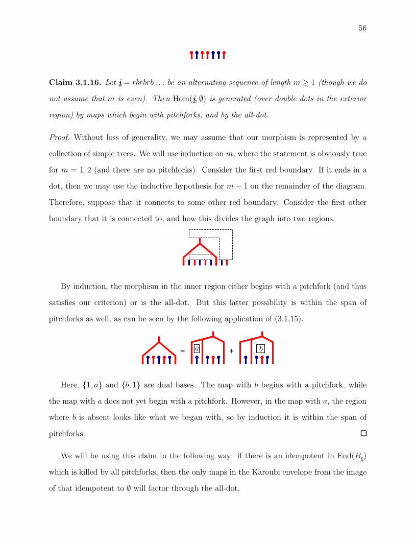
56

Claim 3.1.16. Let i = rbrbrb . . . be an alternating sequence of length m ≥ 1 (though we do

not assume that m is even). Then Hom(i, ∅) is generated (over double dots in the exterior

region) by maps which begin with pitchforks, and by the all-dot.

Proof. Without loss of generality, we may assume that our morphism is represented by a

collection of simple trees. We will use induction on m, where the statement is obviously true

for m = 1, 2 (and there are no pitchforks). Consider the first red boundary. If it ends in a

dot, then we may use the inductive hypothesis for m − 1 on the remainder of the diagram.

Therefore, suppose that it connects to some other red boundary. Consider the first other

boundary that it is connected to, and how this divides the graph into two regions.

By induction, the morphism in the inner region either begins with a pitchfork (and thus

satisfies our criterion) or is the all-dot. But this latter possibility is within the span of

pitchforks as well, as can be seen by the following application of (3.1.15).

= +a b

Here, {1, a} and {b, 1} are dual bases. The map with b begins with a pitchfork, while

the map with a does not yet begin with a pitchfork. However, in the map with a, the region

where b is absent looks like what we began with, so by induction it is within the span of

pitchforks.

We will be using this claim in the following way: if there is an idempotent in End(Bi)

which is killed by all pitchforks, then the only maps in the Karoubi envelope from the image

of that idempotent to ∅ will factor through the all-dot.

57

3.1.6 Temperley-Lieb and Soergel

Fix two colors i and j (among red and blue), and consider the Hom category Hom2T L(i, j).

In particular, this is a non-monoidal category consisting of all diagrams where the rightmost

and leftmost colors are fixed beforehand, and its objects may be thought of as alternating

sequences i of red and blue with fixed extremal colors.

Definition 3.1.17. We now provide a functor from Hom2T L(i, j) to D(∞). On objects it

sends an alternating sequence i to the object i ∈ D(∞). We map the generating morphisms

as follows:

All the morphisms in the image of this functor are degree 0.

Using isotopy, (3.1.2) and the Cartan relation (3.1.12), it is immediate to see that this

functor is well-defined and Z[x, y]-linear. Note that D(∞) contains many non-alternating

sequences i , but only the alternating sequences, and certain degree 0 maps between them,

are in the image of this functor. This functor does not lift to any sort of 2-functor from 2T L

to D(∞), as can be seen in the following example.

Example 3.1.18. but

not

A genuine 2-functor which explains this one will be produced soon, once we discuss

singular Soergel bimodules.

Starting with a diagram in 2T L we can “squeeze” each region into a tree and get the

corresponding Soergel graph, which is maximally connected. Given any maximally connected

58

graph, we may draw lines in the complement of the graph and color each region according

to the graph, to get a crossingless matching in 2T L. This gives a clear bijection between

maximally connected graphs (with the appropriate boundary) and diagrams in 2T L.

Proposition 3.1.19. Let i and j be objects in Hom2T L(i, j) for some colors i, j. Then

the map Hom2T L(i, j) → HomD(∞)(i, j)0, the degree 0 part, is an isomorphism. Moreover,

HomD(∞)(i, j) has no morphisms of negative degree.

Warning: this proof uses the (not-yet-proven) Proposition 3.1.14. Without this Proposi-

tion, the following only proves that the map is surjective.

Proof. The boundary of the Hom space we’re looking at (reading all the way around the

circle) is almost an alternating sequence, except for two repetitions, because both i and j

start with i and end with j. It is clear that this functor gives a bijection from crossing-

less matchings to maximally connected diagrams. That we get precisely the morphisms of

minimal degree 0 is given by Claim 3.1.11, so the Hom space map is surjective. It is also

injective, thanks to Proposition 3.1.14.

The most important consequence of the functor above is that we end up with idempotents

and isomorphisms in (localized) D(∞) and its Karoubi envelope, given by the images of the

projectors and idempotents guaranteed by Proposition 2.3.9. In order to construct these

idempotents we need to be in a 2TL-sufficient ring. For instance, here are the idempotents

which are the images of the first few Jones-Wenzl projectors. These come in two variants:

pictured is the variant which ends with blue.

Example 3.1.20.

−= =

− −

+ +

=

JW1 JW2

JW3

1x

1xy−1

1xy−1

xxy−1

yxy−1

59

Remark 3.1.21. Thanks to Claim 2.3.4, we can describe this map as the unique degree 0 map

killed by any pitchfork on top or bottom.

We may also construct Soergel graphs which correspond to crossingless matchings but

have degree 2 by ignoring the two repetitions from earlier. Here are a few Jones-Wenzl

projectors in this context.

Example 3.1.22. − −

+ +

=

−= =JW1 JW2

JW3

1x

1xy−1

1xy−1

xxy−1

yxy−1

Notation 3.1.23. When we view the Jones-Wenzl projector as a map of degree 2 with

boundary (st)m−1 reading around the circle, we will draw it as a circle labelled by JW . For

instance, JW2 . This map is not rotation-invariant for arbitrary k, so we can not draw it

in a rotation-invariant way.

3.1.7 The Grothendieck Group

Because the Temperley-Lieb algebra subsumes all degree 0 maps, there are no additional

idempotents than those we already know about. All the idempotents which are primitive

(i.e. indecomposable) in the Temperley-Lieb algebra are primitive in D(∞) as well. We may

now transfer everything we know about 2T L (namely Proposition 2.3.10) into a statement

about D(∞). (If we don’t assume Proposition 3.1.14, we can only provide the idempotents

we do know about; we can not claim that there are no additional idempotents, or that these

idempotents are non-zero.)

Theorem 4. Let k be a 2TL-sufficient ring. Then the indecomposables {Bw} in Kar(D(∞)k)

can be labelled by elements w ∈ W∞. The indecomposable Be corresponds to the empty dia-

gram. Each other indecomposable corresponds to the image of the appropriate Jones-Wenzl

60

projector in Bs ⊗ Bt ⊗ . . .. There is an isomorphism from H∞ to the Grothendieck ring of

Kar(D(∞)k) sending bw to [Bw]. For any Soergel ring k, the functor F is an equivalence,

and the indecomposables Bw go to the indecomposable Soergel bimodules that he also labels

Bw.

Proof. We know that Kar(D(∞)k) has objects Bw corresponding to the appropriate Jones-

Wenzl projectors, although we do not know that these objects are non-zero. As before, any

Bi can be decomposed into direct sums of Bw, in the appropriate way, so that we have

a Z [v, v−1]-algebra map H∞ → [Kar(D(∞)k)] sending bw → [Bw]. We now attempt to

pin down the trace map on H induced by D(∞)k. This trace is determined by the graded

rank of Hom(Bw, ∅). Suppose that we can show that Hom(Bw, ∅) is a free Rk-module of

rank 1, generated in degree l(w), so that εD(∞)(bw) = vl(w)grk(R). This would imply that

εD(∞) = ε̃std. Now Lemma 2.4.1 and its corollaries will finish the proof. Also, this allows us

to prove Proposition 3.1.14.

It remains to calculate Hom(Bw, ∅). If w = i is a reduced expression, then this Hom space

can be described as Hom(Bi , ∅) precomposed with the Jones-Wenzl idempotent. However,

by Claim 3.1.16, almost all the maps from Bi to ∅ begin with a pitchfork, which kills the

Jones-Wenzl projector. Therefore, Hom(Bw, ∅) is generated inside Hom(Bi , ∅) by the map

which composes the idempotent with the all-dot. It is at most rank 1 over R (acting by

double dots) with its generator in degree l(w), the degree of the all-dot. Suppose that we

can show that this map is nonzero after applying the functor F . Since R acts freely on Hom

spaces in B, this would imply that Hom(Bw, ∅) must be a free R-module as well.

If one takes the Jones-Wenzl projector JWm and applies dots to every strand, top and

bottom, then one obtains a polynomial. It is immediate that this is precisely the associated

polynomial of the element JWm ∈ 2T L, which is equal to some Lk,l, as discussed in section

2.3.4. This polynomial is nonzero in Rk. Therefore, one also gets a nonzero answer when

applying F to the Jones-Wenzl projector with dots just on the top. This concludes the

proof.

61

3.2 Singular Soergel Bimodules: m = ∞

3.2.1 Definitions

Definition 3.2.1. A singular Soergel graph or Soergel 1-manifold diagram for m = ∞

is (almost) an isotopy class of a particular kind of 1-manifold with boundary, properly

embedded in the planar strip (so that the boundary of the graph is always embedded in

the boundary of the strip). The regions cut out by this 1-manifold are labelled by finitary

parabolic subsets {e, s, t}, in such a way that s never abuts t. Soergel 1-manifold diagrams are

graded, where the degree of a clockwise cup or cap is +1, and the degree of a counterclockwise

cup or cap is −1.

In addition to labeling regions, one can color and orient the 1-manifold itself. A line

can be colored s or t, and separates two regions whose label differs by that element. The

orientation is such that the larger parabolic subset is on the right hand of the 1-manifold.

The boundary of the graph gives two sequences of colored oriented points, the top and bottom

boundary. Not every oriented colored 1-manifold gives rise to a consistent labeling of regions.

If there is no ambiguity, we shorten the name to “Soergel diagram.” We think of a Soergel

diagram as being the data of two oriented 1-manifolds, one blue and one red, which are not

allowed to overlap. This is different from the m < ∞ case, where they are allowed to intersect

transversely. Note that the degree of a diagram is not isotopy invariant, so that rotating a

relation will give a relation in a different degree. This is the only sense in which we do not

consider Soergel diagrams as isotopy classes.

Definition 3.2.2. Let D(∞) be the 2-category defined as follows. The objects are {e, s, t}.

The 1-morphisms are generated by maps from e to s and back, and maps e to t and back.

A path in the object space (like sesetes) uniquely specifies a 1-morphism. The 2-morphism

space between 1-morphisms is the free Z[x, y, (xy−4)−1]-module spanned by Soergel diagrams

with the appropriate boundary, modulo the relations below. Hom spaces will be graded by

the degree of the Soergel diagrams.

62

The first two relations hold for both colors:

= 0 (3.2.1)

+ = 2 (3.2.2)

= 2 (3.2.3)

The next relations, along with (3.2.2) above, are called the circle forcing relations.

+= − xx (3.2.4)

+= − yy (3.2.5)

Finally, along with (3.2.3) we have the Cartan relations:

= x (3.2.6)

= y (3.2.7)

The forcing relations immediately imply the circle sliding relations.

−= 2−2 xx (3.2.8)

63

−= 2−2 y y (3.2.9)

Given (3.2.3) and the circle forcing relations, the remaining Cartan relations are redun-

dant if we invert 2. Also, one can demonstrate using (3.2.2) that the left side of (3.2.3)

squares to twice itself, so that (3.2.3) is already implied if we desire our endomorphism ring

to be a domain.

One should think of clockwise circles as the new double dots. That is, they give a way for

Ru to act in any e region. Placing a polynomial inside a counterclockwise circle surrounded

by region i is effectively taking ∂i of that polynomial. The map ∂i is surjective, so this gives

an action of Ri in a region labelled i. We will still use a box labelled f to represent the

polynomial f , and if it appears inside a blue region then it must be in Rs.

Given this notation (which is only consistent because of the relations above) we may

rewrite the circle sliding, circle forcing, and Cartan relations as follows:

= ff when f ∈ Rs (3.2.10)

= =fs ft (3.2.11)

=f ∂s(f) (3.2.12)

= ∆s (3.2.13)

The map ∆s in (3.2.13) is the comultiplication element in Bs, as described in section

2.2.4.

64

3.2.2 Functors

Definition 3.2.3. We give a functor ι : D(∞) → HomD(∞)(e, e). On objects, it sends s to

the path ese and t to the path ete. We define the functor on generators:

Claim 3.2.4. The above definition gives a well-defined functor.

Proof. Both categories only consider pictures up to isotopy, so we may ignore questions of

isotopy invariance. Relations (3.1.2) and (3.1.1) also correspond to mere isotopies in D(∞),

and relation (3.1.3) corresponds to relation (3.2.1). A double dot in D(∞) goes to a clockwise

circle in D(∞). The correspondence between the dot sliding and forcing relations of D(∞)

and the circle sliding and forcing relations of D(∞) is clear.

Proposition 3.2.5. The functor ι is an isomorphism of categories.

Proof. Clearly any path from e to itself will be composed out of the smaller loops ese and

ete, so that we have a bijection of objects between sequences of indices i and sequences

of paths eie. To give a functor in the reverse direction, take any morphism in Hom(e, e)

and deformation retract the shaded regions to some graph with the appropriate boundaries.

Which graph you choose is irrelevant because of relations (3.1.2) and (3.1.1). The same

correspondence of relations in the previous proof shows that all of the relations in D(∞)

go to zero in D(∞). Perhaps the only subtlety is relation (3.2.1), which is not phrased as

within Hom(e, e). However, any instance of a counterclockwise circle within Hom(e, e) will

clearly be sent to an empty cycle within a Soergel graph, and this is zero. The same can be

said about the Cartan relations and their previous counterparts. Therefore this functor is

well-defined, and clearly yields the inverse functor.

Definition 3.2.6. We give a (strict) 2-functor F : D(∞) → Bu to the 2-category of singular

Soergel bimodules. This 2-functor is the identity on objects, so that we think of ule as

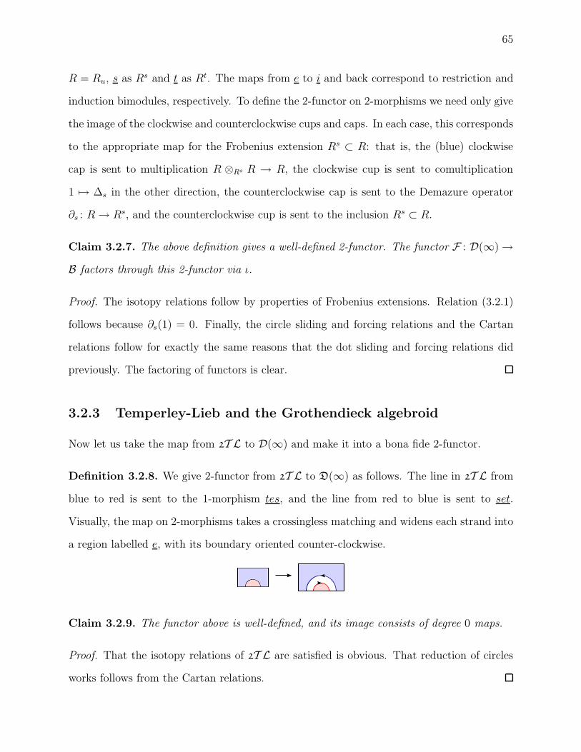
65

R = Ru, s as Rs and t as Rt. The maps from e to i and back correspond to restriction and

induction bimodules, respectively. To define the 2-functor on 2-morphisms we need only give

the image of the clockwise and counterclockwise cups and caps. In each case, this corresponds

to the appropriate map for the Frobenius extension Rs ⊂ R: that is, the (blue) clockwise

cap is sent to multiplication R ⊗Rs R → R, the clockwise cup is sent to comultiplication

1 7→ ∆s in the other direction, the counterclockwise cap is sent to the Demazure operator

∂s : R → Rs, and the counterclockwise cup is sent to the inclusion Rs ⊂ R.

Claim 3.2.7. The above definition gives a well-defined 2-functor. The functor F : D(∞) →

B factors through this 2-functor via ι.

Proof. The isotopy relations follow by properties of Frobenius extensions. Relation (3.2.1)

follows because ∂s(1) = 0. Finally, the circle sliding and forcing relations and the Cartan

relations follow for exactly the same reasons that the dot sliding and forcing relations did

previously. The factoring of functors is clear.

3.2.3 Temperley-Lieb and the Grothendieck algebroid

Now let us take the map from 2T L to D(∞) and make it into a bona fide 2-functor.

Definition 3.2.8. We give 2-functor from 2T L to D(∞) as follows. The line in 2T L from

blue to red is sent to the 1-morphism tes, and the line from red to blue is sent to set.

Visually, the map on 2-morphisms takes a crossingless matching and widens each strand into

a region labelled e, with its boundary oriented counter-clockwise.

Claim 3.2.9. The functor above is well-defined, and its image consists of degree 0 maps.

Proof. That the isotopy relations of 2T L are satisfied is obvious. That reduction of circles

works follows from the Cartan relations.

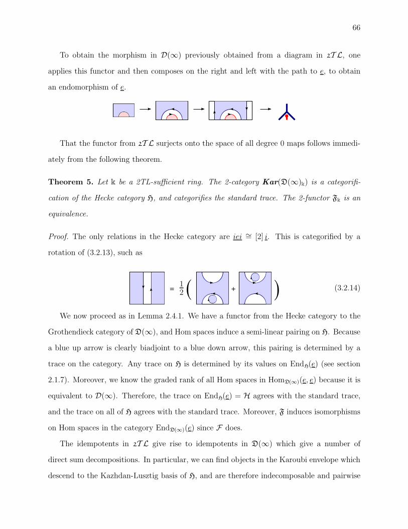
66

To obtain the morphism in D(∞) previously obtained from a diagram in 2T L, one

applies this functor and then composes on the right and left with the path to e, to obtain

an endomorphism of e.

That the functor from 2T L surjects onto the space of all degree 0 maps follows immedi-

ately from the following theorem.

Theorem 5. Let k be a 2TL-sufficient ring. The 2-category Kar(D(∞)k) is a categorifi-

cation of the Hecke category H, and categorifies the standard trace. The 2-functor Fk is an

equivalence.

Proof. The only relations in the Hecke category are iei ∼= [2] i. This is categorified by a

rotation of (3.2.13), such as

+= ( )12

(3.2.14)

We now proceed as in Lemma 2.4.1. We have a functor from the Hecke category to the

Grothendieck category of D(∞), and Hom spaces induce a semi-linear pairing on H. Because

a blue up arrow is clearly biadjoint to a blue down arrow, this pairing is determined by a

trace on the category. Any trace on H is determined by its values on EndH(e) (see section

2.1.7). Moreover, we know the graded rank of all Hom spaces in HomD(∞)(e, e) because it is

equivalent to D(∞). Therefore, the trace on EndH(e) = H agrees with the standard trace,

and the trace on all of H agrees with the standard trace. Moreover, F induces isomorphisms

on Hom spaces in the category EndD(∞)(e) since F does.

The idempotents in 2T L give rise to idempotents in D(∞) which give a number of

direct sum decompositions. In particular, we can find objects in the Karoubi envelope which

descend to the Kazhdan-Lusztig basis of H, and are therefore indecomposable and pairwise

67

non-isomorphic. Therefore the map from H to the Grothendieck category is an equivalence

of categories. Similar arguments show that F is an equivalence.

3.2.4 Induced Modules

Corollary 3.2.10. Over a 2TL-sufficient ring k, the category HomD(∞)(e, s) categorifies the

left ideal of bs, which is the induced module from the trivial representation of Hs. The module

action is categorified by the monoidal action of EndD(∞)(e) = D(∞).

Note that this Hom category can easily be described using a slight modification of D(∞),

in a precise analogy to Chapter 4 in [5]. One may draw the usual Soergel graphs but require

that they end in a “blue region”. One adds a new morphism corresponding to a trivalent

vertex with the blue region, and imposes relations corresponding to (3.1.1) and (3.1.2).

Explicitly, the new generator is . The new relations are

= = (3.2.15)

Any usual Soergel graph, with the usual Soergel relations, may be drawn to the left of the

blue region.

It is quite easy to provide the equivalence of categories between this diagrammatic cate-

gory and HomD(∞)(e, s), in analogy to the functor ι above.

68

Chapter 4

Dihedral Diagrammatics: m < ∞

When m < ∞ we know that that bsts... = btst.... In Kar(D(∞)) we have found two idem-

potents corresponding to Bsts... and Btst..., and requiring the images of these idempotents to

be isomorphic will give a category equipped with map from Hm to its Grothendieck algebra.

Therefore, to define Kar(Dm) we could formally add this isomorphism as a new generator.

Instead we do this same thing before taking the Karoubi envelope, modifying D(∞) into

a category Dm by adding maps from Bs ⊗ Bt ⊗ Bs ⊗ . . . → Bt ⊗ Bs ⊗ Bt ⊗ . . . and back

which interact in a precise way with the various idempotents. In order for this category to

be consistently defined, we must change base to a ring km where the action of W∞ on h

descends to Wm. Note that changing base for D(∞) would not be sufficient: one must still

add this new morphism.

Let i and j be two sequences which are reduced expressions for elements of Wm and live

as objects in some Hom2T L(i, j) (so that they both end with i and start with j). Then it is

still true that Hom2T L(i , j ) surjects onto the degree 0 part of HomDm(i , j ). However, while

in D(∞) these are the only degree 0 maps between reduced expressions in the entire category,

in Dm there is now an additional degree 0 map from sts . . . to tst . . .. This map could not

correspond to anything in 2T L because the source and target objects do not match up!

Neither is this some sort of 2-categorical extension of 2T L, because objects are inconsistent.

69

What we have is an extension of 2T L but not as a 2-category. We have not encountered

this sort of categorical extension before and without further examples we are unsure what

general structure to define to encapsulate it.

What is remarkable is that the relations in Dm are truly uniform over all m. That is,

abstracting the Jones-Wenzl projector into a map JWm depending on m, the relations have

a very simple form which does not depend on m. Of course, the morphism JWm and its

behavior does depend strongly on m.

4.1 The category Dm

4.1.1 Definitions

Definition 4.1.1. A Soergel graph for m < ∞ is an isotopy class of a particular kind of

graph with boundary, properly embedded in the planar strip (so that the boundary of the

graph is always embedded in the boundary of the strip). The edges in this graph are colored

by either s or t. The vertices in this graph are either univalent (dots), trivalent with all

three adjoining edges having the same color, or 2m-valent with alternating edge colors. The

boundary of the graph gives two sequences of colors, the top and bottom boundary. Soergel

graphs have a degree, where trivalent vertices have degree −1, dots have degree 1, and

2m-valent vertices have degree 0.

When there is no ambiguity we refer to a Soergel graph for m merely as a “graph.” If we

want to talk about Soergel graphs for m = ∞ again, we will say so explicitly.

Fix a base ring km which is m-symmetric and 2TLm−1-sufficient.

Definition 4.1.2. Let Dm be the km-linear monoidal category defined herein. The objects

will be finite sequences i = i1i2 . . . id of indices s and t, with a monoidal structure given

by concatenation. The space HomDm(i , j ) will be the free km-module generated by Soergel

graphs with bottom boundary i and top boundary j , modulo the relations below. Hom

70

spaces will be graded by the degree of the Soergel graphs.

We have all the relations that define D(∞) (see section 3.1.1) as well as two new relations,

called the two-color relations, found in equations (4.1.1) and (4.1.2). They hold with the

colors switched as well. It is difficult to draw these relations for all m at once, since the

number of strands entering a vertex changes. A circle labelled JW contains the Jones-Wenzl

projector JWm−1 as a degree 2 map (see Notation 3.1.23), and a circle labelled v contains

the 2m-valent vertex. A sequence of a few purple lines will indicate an alternating sequence

of red and blue lines of the appropriate length (depending on m).

The new relations are two-color associativity :

m=2

m=3

m=4

=

=

=

m even

m odd

=

=

vv

v

v

vv

(4.1.1)

and dotting the vertex :

m=2

m=3

m=4

=

=

m arbitrary

=

= − yv JW

+ +

− y − x

(4.1.2)

Each figure has some examples, with the 2m-valent vertex in these relations circled. Note

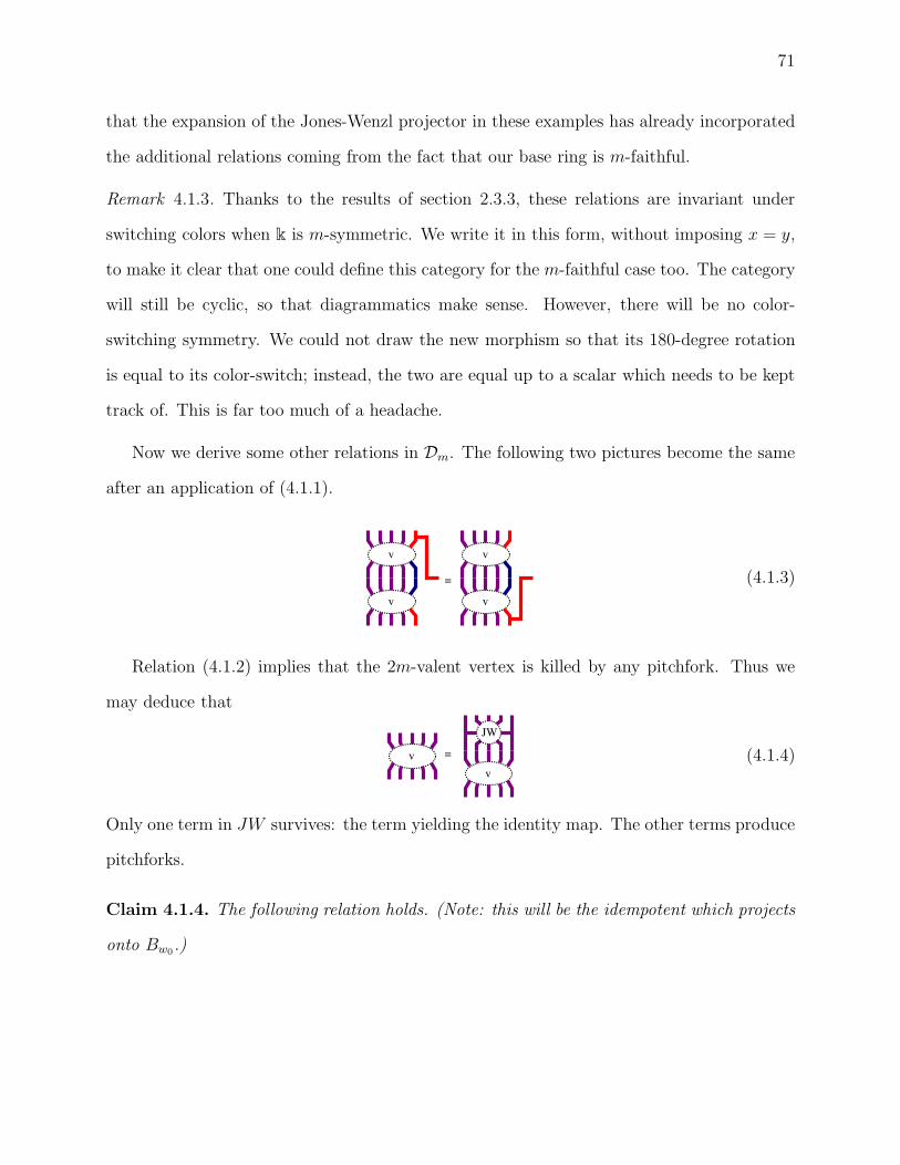
71

that the expansion of the Jones-Wenzl projector in these examples has already incorporated

the additional relations coming from the fact that our base ring is m-faithful.

Remark 4.1.3. Thanks to the results of section 2.3.3, these relations are invariant under

switching colors when k is m-symmetric. We write it in this form, without imposing x = y,

to make it clear that one could define this category for the m-faithful case too. The category

will still be cyclic, so that diagrammatics make sense. However, there will be no color-

switching symmetry. We could not draw the new morphism so that its 180-degree rotation

is equal to its color-switch; instead, the two are equal up to a scalar which needs to be kept

track of. This is far too much of a headache.

Now we derive some other relations in Dm. The following two pictures become the same

after an application of (4.1.1).

=

v

v

v

v

(4.1.3)

Relation (4.1.2) implies that the 2m-valent vertex is killed by any pitchfork. Thus we

may deduce that

=v

JW

v

(4.1.4)

Only one term in JW survives: the term yielding the identity map. The other terms produce

pitchforks.

Claim 4.1.4. The following relation holds. (Note: this will be the idempotent which projects

onto Bw0.)

72

m=2

m=3

m=4

=

=

m even=

= − y

v

JW

− y − x

+ +

v

m odd=

v

JWv

(4.1.5)

Proof. Using in order: (3.1.2), (4.1.3), (4.1.2), (4.1.4), and (4.1.2). The coloration is as

though m is even, although if m is odd one only need change the color on the leftmost

strands.

=

v

v

v

v

=

v

v

=

v

JW

= v = JW

We invite the reader to compare relation (4.1.1) with relation (3.7) in [5].

4.1.2 The Grothendieck group

Now let us assume that km is m-symmetric and 2TLm−1-sufficient.

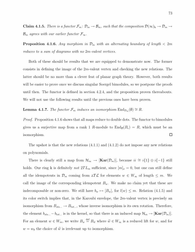
73

Claim 4.1.5. There is a functor Fm : Dm → Bm, such that the composition D(∞)k → Dm →

Bm agrees with our earlier functor F∞.

Proposition 4.1.6. Any morphism in Dm with an alternating boundary of length < 2m

reduces to a sum of diagrams with no 2m-valent vertices.

Both of these should be results that we are equipped to demonstrate now. The former

consists in defining the image of the 2m-valent vertex and checking the new relations. The

latter should be no more than a clever feat of planar graph theory. However, both results

will be easier to prove once we discuss singular Soergel bimodules, so we postpone the proofs

until then. The functor is defined in section 4.2.4, and the proposition proven thereabouts.

We will not use the following results until the previous ones have been proven.

Lemma 4.1.7. The functor Fm induces an isomorphism EndDm(∅) ∼= R.

Proof. Proposition 4.1.6 shows that all maps reduce to double dots. The functor to bimodules

gives us a surjective map from a rank 1 R-module to EndB(Be) = R, which must be an

isomorphism.

The upshot is that the new relations (4.1.1) and (4.1.2) do not impose any new relations

on polynomials.

There is clearly still a map from H∞ → [Kar(Dm)], because ii ∼= i{1} ⊕ i{−1} still

holds. Our ring k is definitely not 2TLm sufficient, since [m]x = 0, but one can still define

all the idempotents in Dm coming from 2T L for elements w ∈ W∞ of length ≤ m. We

call the image of the corresponding idempotent Bw. We make no claim yet that these are

indecomposable or non-zero. We still have bw 7→ [Bw], for l(w) ≤ m. Relation (4.1.5) and

its color switch implies that, in the Karoubi envelope, the 2m-valent vertex is precisely an

isomorphism from Bsts... → Btst..., whose inverse isomorphism is its own rotation. Therefore,

the element bsts... − btst... is in the kernel, so that there is an induced map Hm → [Kar(Dm)].

For an element w ∈ Wm, we write Bwdef= B ew where w̃ ∈ W∞ is a reduced lift for w, and for

w = w0 the choice of w̃ is irrelevant up to isomorphism.

74

Theorem 6. Suppose that k is m-symmetric and 2TLm−1-sufficient. There is an isomor-

phism Hm → [Kar(Dm)] which sends bs → [Bs], bw0 → [Bw0], and in general bw → [Bw].

This categorifies the standard trace map. For any Soergel ring, Fm is an equivalence of

categories, sending indecomposables Bw to Bw.

Proof. That a map Hm → [Kar(Dm)] exists and sends the elements to their images as stated

is now clear. We have not shown that the map is injective or surjective (or that the right

hand side is nonzero) but nonetheless there is induced on Hm a trace map. It remains to

show that this trace map is the standard trace map, for this will imply that all the objects

mentioned are nonzero, pairwise non-isomorphic, and indecomposable. Again, the trace map

can be computed by calculating Hom(Bw, ∅) for all w ∈ Wm, which is computed by looking

at maps Bi → ∅ for reduced expressions which are unchanged by composition with the

appropriate idempotent.

Let i be an alternating sequence of length ≤ m, representing a reduced expression.

Proposition 4.1.6 implies that every diagram representing a map from Hom(Bi , ∅) can be

reduced to a linear combination of diagrams involving only dots and trivalent vertices. We

can use the exact same arguments as in Theorem 4 to show that the only possible map which

wouldn’t kill the idempotent is the all-dot. We have already calculated the polynomial which

appears when you apply the all-dot on both sides to a Jones-Wenzl projector, and computed

that this polynomial is nonzero (thanks to Lemma 4.1.7). The remainder of the proof

continues exactly as in Theorem 4, using the appropriate analog of Lemma 2.4.1.

4.2 Singular Soergel Bimodules: m < ∞

4.2.1 Definitions

Definition 4.2.1. A singular Soergel graph or Soergel 1-manifold diagram for m is (almost)

an isotopy class of two oriented 1-manifolds with boundary properly embedded in the planar

strip, one of each color, which can only intersect transversely. Moreover, there must be a

75

Figure 4.1: Degrees of Soergel diagrams

degreegenerator

+1

−1

m−1

1−m

0

m−2

consistent labeling of the regions between these edges. Regions may be labelled by parabolic

subsets {e, s, t, W}. A line can be colored s or t, and separates two regions whose label

differs by that element. The orientation is such that the larger parabolic subset is on the

right hand of the 1-manifold. The boundary of the graph gives two sequences of colored

oriented points, the top and bottom boundary. Not every oriented colored 1-manifold gives

rise to a consistent labeling of regions. Soergel 1-manifold diagrams are graded as in figure

4.1.

If there is no ambiguity, we shorten the name to “Soergel diagram.” One can remember

that the degree of a cup or cap is always “in minus out,” regardless of orientation, where

we associate to a region the length of the longest element of the corresponding parabolic

subgroup (which is 0, 1, or m). The degree of a sideways crossing is “big minus middle

minus middle plus small,” which in this case is always m − 1 − 1 + 0 = m − 2. Note that

the degree of a diagram is not an isotopy invariant. This is the only sense in which we do

not consider Soergel diagrams as isotopy classes. The degree of morphisms is also the only

place where m enters into the definition.

A picture is often worth a thousand words. We will try to be very clear about what

we refer to in a picture. “Lines” or “strands” will refer to sections of the red or the blue

1-manifold. A “blue circle” will denote a blue line in the shape of a circle (which can separate

76

either a red region from a purple one, or blue from white), while a “blue circular region” will

refer a blue region enclosed by a circle of indefinite color. We might refer to a 1-morphism by

the sequence of lines comprising it (i.e. “red up blue down”) or by the colors of the regions

(i.e. “red purple blue”). Purple designates W . We refer to a diagram without any purple

regions as an ∞-diagram.

Let km be m-symmetric and 2TLm−1-sufficient.

Definition 4.2.2. Let Dm be the 2-category defined as follows. The objects are {e, s, t, W},

thought of as parabolic subsets. The 1-morphisms are generated by maps from I to J and

whenever their difference is a single element. A path in the object space (like sesWtWse)

uniquely specifies a 1-morphism. The 2-morphism space between 1-morphisms is the free

k-module spanned by Soergel diagrams with the appropriate boundary, modulo the relations

below. Hom spaces will be graded by the degree of Soergel diagrams.

We have all the relations present in D(∞) (see section 3.2.1), which give all the relations

between ∞-diagrams. This means that we have a functor D(∞) → Dm, and we already

know how to place an (appropriately invariant) polynomial inside a region labelled e, s, or t.

We will write some of the remaining relations in terms of polynomials, instead of expressing

them in terms of circles. The first relation gives us a way of writing elements of RW inside

a region labelled W , since ∂sW is surjective.

=f ∂sW (f) (4.2.1)

=L

fs(4.2.2)

= ff when f ∈ RW (4.2.3)

= ∆sW (4.2.4)

77

These relations hold with colors switched, and represent standard relations for a Frobenius

extension. The element ∆sW ∈ Rs ⊗RW Rs is described in section 2.2.5. Because of the

relations, there is a map from Rs ⊗RW Rs → End(sWs) given by placing boxes in the right

and left regions. Similar actions are represented by boxes which cross multiple lines: they

represent linear combinations of diagrams with boxes on each side, not in the middle.

The next relation, an analog of Reidemeister II, says that like-oriented strands can be

pulled apart.

= (4.2.5)

We also have non-oriented Reidemeister II relations. The element ∂∆st represents the

element ∆sW (1) ⊗ ∂t(∆

sW (2)) = ∂s(∆

tW (1)) ⊗ ∆t

W (2) ∈ Rs ⊗W Rt, as described in section 2.2.5.

= ∂∆st (4.2.6)

= L

fsft(4.2.7)

All of the above relations hold in generality for squares of Frobenius extensions. See [9]

for more details.

There is only one truly interesting relation, unique to the dihedral group. This relation

starts with m − 1 alternating arcs of each color, oriented around an inner purple region. It

replaces this with an ∞-diagram, the image of JWm−1 under the functor 2T L → D(∞) →

Dm.

78

m=2

m=3

m=4

m arbitrary

− −

=

= −

= + +

JW=

x

y

y

(4.2.8)

4.2.2 Graph simplifications

Remember that the word “polynomial” in this context refers to a linear combination of

certain configurations of circles, which we know gives a map from some invariant ring RI

to Hom spaces in Dm. We have not yet shown that this map is injective, or even that

polynomials are non-zero.

Lemma 4.2.3. (The Circle Removal Lemma) Any morphism in Dm can be represented

as a linear combination of diagrams with no closed components of either color, but with

polynomials in arbitrary regions. Any Soergel diagram with empty boundary reduces to a

polynomial.

Proof. This is proven in [9], and is a general statement about squares of Frobenius algebras.

In other words, a collection of nested circles easily evaluates to a polynomial using the

relations above, and a more complicated system of overlapping circles may be pulled apart

using Reidemeister II moves, and reduced to a polynomial as well. Note that this lemma

holds regardless of the color of the region on the boundary, so that a closed Soergel diagram

79

in a white region evaluates to a polynomial in R, and a closed Soergel diagram in a blue

region becomes a polynomial in Rs.

Now we attempt to simplify more complicated graphs with boundary.

Notation 4.2.4. When given k alternating arcs of each color oriented around an inner

purple region as in (4.2.8), we will denote the map by vk. Our interesting relation says that

vk = JWk only for k = m − 1, not for arbitrary k. In the example below, k = 6.

= vk

The map vk can be oriented in many ways, and its orientation determines its degree.

However, when oriented as a map from esetese . . . to etesete . . ., it will have degree 2(m−k).

We let v0 denote a purple circle in a blue annulus in a white region (or purple in red in white,

these are equal). Using the relations above, v0 is equal to L. It is obvious that any purple

region which does not meet the boundary must have a neighborhood equal to vk for some

k ≥ 1, or simply be a purple circular region.

If we place a colored cap on one of the colored sections of the boundary of vk for k ≥ 1, we

can use (4.2.5) to pull two strands apart, and obtain vk−1 with an added “trivalent vertex.”

=vk vk−1(4.2.9)

From this, it is easy to show that “pitchforks” kill vk, and double capping vk will yield vk−1.

80

= = 0vkvk vk−1

Relation (4.2.8) says that vm−1 can be de-purplified, i.e. rewritten as a sum of ∞-

diagrams. Therefore, any vk for k ≤ m − 1 can also be de-purplified. After all, vk equals

vm−1 with a number of cups attached, and will be equal to JWm−1 with a number of cups

attached. Note that relation (4.2.7) is actually a statement about v1; in fact, this relation is

redundant, merely stating that the RHS is what one obtains when one caps JWm−1 almost

everywhere.

Warning: Remember that caps do not kill JWm−1 in this context, only the analogs of

pitchforks kill JWm−1. Also, capping off JWm−1 certainly does not yield JWk for k < m−1.

For k > m − 1, one can not use (4.2.8) to de-purplify vk. In fact, vm is the smallest

diagram which is not in the span of ∞-diagrams, and will be the image of the 2m-valent

vertex under the functor from Dm to Dm to be defined. Thankfully, all vk for k > m can be

expressed using only vm. In order to show this, we introduce an auxiliary map..

For k ≥ 2, consider the following maps Ck of degree 2(m−k), where the number of circles

is k − 2:

C6

=

C5

=

Claim 4.2.5. When m = k (so that this map is degree 0), we have

Cm

=

m odd m even

or(4.2.10)

81

Proof. Using the circle elimination lemma as well as polynomial manipulation rules, we see

that this map must reduce to some polynomial in Rs ⊗RW Rt. For degree reasons this

polynomial is a scalar, so we must only check that this scalar is 1. In fact, the derivation

goes as follows, for the case m = 4:

=

The first step is to apply (4.2.6) to obtain a sum of diagrams with boxes in the rightmost

blue region, and a box in the red region as pictured. However, only one term in this sum

survives: the term where the box in the rightmost region is 1. Were the box in the rightmost

region of degree > 0, then the diagram to the left of that region would have to reduce to

a polynomial of negative degree, equal to 0. Therefore cm is equal to a single diagram as

pictured, where if f is the polynomial dual to 1 under ∂sW , then the element in the box is

∂t(f).

Now we apply (3.2.10), (4.2.5), and (3.2.12) until the diagram only has a box in the left

region.

= = =

= = =

We place ∂t(f) in the box in every diagram on the second row. But then ∂s(∂t(f)) appears

in the box on the third row, and ∂t(∂s(∂t(f))) on the fourth row (and so forth, for m > 4).

Therefore, the final polynomial appearing is ∂sW (f), which is 1.

Now we use Cm to help understand vk.

82

Claim 4.2.6. For every k ≥ m we have

=

vk

vk+1

vm

(4.2.11)

The example here has k = 4 and m = 3, although the typical example is similar. When m is

even, the new side colors are different rather than the same.

Proof. The example below should make the general proof clear.

= =cm

Remark 4.2.7. In fact, ck = 0 for k > m, since it reduces to a polynomial of negative degree.

A similar proof shows that replacing vm with vl for any l > m in the above diagram would

yield 0. In other words, if any two purple regions vk and vl are connected by more than m

“colored bands,” then the result is 0.

Lemma 4.2.8. Suppose that a diagram in Dm has no purple appearing on the boundary.

Then it reduces to linear combinations of diagrams generated by ∞-diagrams and vm.

Proof. Let us note that any polynomial may always be slid to a lighter region (i.e. purple

to blue to white), and polynomials in blue or red or white regions can be expressed in terms

of ∞-diagrams. Now suppose that there is a purple region in the diagram. If this purple

83

region is a circular region, it reduces to a polynomial by (4.2.2). If this purple region is vk

for 1 ≤ k < m then we may de-purplify it, as previously discussed. If this purple region is

vk for k ≥ m then we may express it using only copies of vm, by using (4.2.11) iteratively.

This procedure will strictly decrease the number of purple regions labelled by k 6= m, and

therefore we may eliminate all such purple regions.

Note that if there is no purple on the boundary, then we are dealing with objects that

may as well live inside D(∞). In particular, suppose that there is some white region on

the boundary. Then, reading around the boundary, the colors of regions must be of the

form ei1ei2ei3e . . . for some sequence i , and corresponds to some Bott-Samelson bimodule.

Using the relations of D(∞), we may as well remove repetitions in the sequence i using the

standard isomorphisms.

Corollary 4.2.9. Suppose that a diagram has boundary ei1ei2e . . . eide when reading around

the boundary of the disk, where i is an alternating sequence of length d. If d < 2m then

every diagram with that boundary can be de-purplified.

Proof. This is a simple consequence of the circle removal lemma. We may reduce the diagram

to a diagram with no closed 1-manifold components of either color, so the only components

come from those on the boundary. Clearly then, there are not enough components for vm

to appear in the diagram (or vk for k ≥ m), unless different strands in the boundary of vm

are connected to each other. However, if any two strands in vm are connected to each other,

then by simple planar arguments there must be a cup somewhere, implying that vm reduces

to vm−1 and eventually to ∞-diagrams.

4.2.3 Comparison to the non-singular case

Definition 4.2.10. We give a functor ιm : Dm → HomDm(e, e). On objects, it sends s to

the path ese and t to the path ete. We define the functor on dots and trivalent vertices as

in Definition 3.2.3. We define the functor on the 2m-valent vertex here.

84

vm

Claim 4.2.11. The above definition gives a well-defined functor.

Proof. Because this was true for ι : D(∞) → HomD(∞)(1, 1), we need only check the relations

involving 6-valent vertices, (4.1.1) and (4.1.2). Both categories only consider pictures up to

isotopy, so we may ignore questions of isotopy invariance. Relation (4.1.2) follows from

(4.2.9) and (4.2.8). Relation (4.1.1) follows from

= = = vmvmvmvmvm vm+1

Claim 4.2.12. This functor is full.

Proof. This is precisely the statement of Lemma 4.2.8.

We will also show that this functor is faithful, although it is not essentially surjective,

because there are loops based at e which pass through W . The functor is an equivalence

after passing to the Karoubi envelope. Once we have shown that the functor is faithful,

Corollary 4.2.9 will give an immediate proof of Proposition 4.1.6.

4.2.4 The functor to bimodules

Definition 4.2.13. Let km be m-symmetric and 2TLm−1-sufficient. We define a 2-functor

Fm : Dm → Bm as follows. On objects it is the identity, and on 1-morphisms it sends the

map from I to J for I ⊂ J to the restriction bimodule RI (as an RJ − RI-bimodule), and

85

it sends the map from J to I to the induction bimodule RI (as an RI − RJ -bimodule).

Cups and caps are sent to the appropriate maps of Frobenius algebras, as discussed in

sections 2.2.4 and 2.2.5. The upwards-pointing crossing goes to the canonical isomorphism

R ⊗Rs Rs ⊗RW RW ∼= R ⊗Rt Rt ⊗RW RW , which are both R as an R − RW -bimodule.

Similarly, the downwards-pointing crossing is a canonical isomorphism between R and itself

as an RW − R-bimodule. The sideways crossings are maps between R and Rs ⊗RW Rt as

Rs − Rt-bimodules, which are either multiplication or the map f → ∆sW,(1) ⊗ ∂t(f∆s

W,(2))

discussed in section 2.2.5.

Proposition 4.2.14. This 2-functor is well-defined.

Proof. We must check the relations of the category, as well as isotopy relations. Almost

all these relations (including the isotopy relations) hold in more generality for squares of

Frobenius extensions, and they are proven in [9]. The only relation that needs to be checked

is (4.2.8), expressing vm−1 as JWm−1. Thankfully, we understand how Hom spaces work in

Bm. We may view the map vm−1 as a map from Bs ⊗ Bt ⊗ . . .︸ ︷︷ ︸2(m−1)

→ R, which is killed by

every pitchfork and has minimal degree. We have already seen that the space of such maps

is 1-dimensional, and that placing a dot on every Bi (which corresponds in the singular

world to placing caps on every colored band) gives an injective map from this 1-dimensional

space into the endomorphisms of R (i.e. R itself). Therefore, we need only show that vm−1

and JWm−1 produce the same polynomial when capped off everywhere. But we have already

shown that vm−1 capped off everywhere is v0 = µW = L, while JWm−1 capped off everywhere

is its associated polynomial, which is also L (see section 2.3.4).

Corollary 4.2.15. For any parabolic subset, EndDm(I) ∼= RI .

Proof. We have already seen that all such diagrams reduce to polynomials, and the existence

of the functor implies that there can be no additional relations between polynomials.

In fact, we can make this corollary even stronger, in light of Corollary 4.2.9.

86

Corollary 4.2.16. For i an alternating sequence of length < 2m and X the corresponding 1-

morphism ei1ei2e . . . eide in Dm or D(∞), the natural 2-functor from D(∞)k → Dm induces

isomorphisms on Hom(X, e).

Proof. The map has already been shown to be surjective. It must be injective, since the

functor from D(∞)k → Bk is an equivalence, and factors through Dm.

This saves us from having to calculate explicitly the bimodule morphism corresponding

to the 2m-valent vertex.

Definition 4.2.17. We define the functor Fm : Dm → Bm as the composition of ιm and Fm.

Clearly this functor agrees with F∞ on the image of D(∞) in Dm, since Fm agrees with

F∞ on ∞-diagrams.

4.2.5 The Grothendieck Algebroid

Theorem 7. The 2-category Kar(Dm) categorifies the Hecke algebroid Hm. If km is a

Soergel ring then Fm is an equivalence after passage to the Karoubi envelope. In addition,

ιm is fully faithful and Fm is an equivalence of categories.

Proof. First we show that there is a map from Hm to the Grothendieck category of Dm.

We have presented Hm by generators and relations in section 2.1.6, and it is clear what

happens to the generators, so we need only check the relations. Equation (2.1.7) follows

from the modification (3.2.14) of (3.2.13) as in D(∞), and equation (2.1.8) follows from the

equivalent modification of (4.2.4). The isomorphism esW ∼= etW required by equation (2.1.9)

is realized by the upwards-pointing crossing, and the same for (2.1.10) and the downwards-

pointing crossing. Finally, the most interesting relation is (2.1.11). This is implied by the

decompositions in 2T L, after applying the functor to D(∞).

Therefore, Dm induces a trace on Hm, which can be identified by its values on EndHm(e) =

Hm. These in turn are determined by the graded dimensions of the Hom spaces specified in

87

Corollary 4.2.16, which agree with the graded ranks of Hom spaces in D(∞). Therefore, the

trace induced by Dm is equal to the standard trace. The remaining arguments proceed as

usual.

4.3 Thickening

4.3.1 Diagrams for BgBS

Recall that BgBS is the full subcategory of B monoidally generated by Bs, Bt, and BW . We

present this category diagrammatically, in precise analogy with [5], chapter 3.5.

Definition 4.3.1. A thick Soergel graph has edges labelled either s, t, or W (purple). The

new vertices (compared to a Soergel graph) are: trivalent with 3 purple edges (degree −m);

trivalent with two purple and one other (degree −1); univalent with one purple (degree m);

and m+1-valent with one purple edge and the remainder alternating between s and t (degree

0).

Definition 4.3.2. The category Dm,gBS has morphisms given by thick Soergel graphs, with

the relations of Dm as well as the following relations.

JW= = (4.3.1)

= = (4.3.2)

= (4.3.3)

88

=(4.3.4)

Relation (4.3.1) identifies the purple line as the image of the idempotent which picks out

BW inside Bs⊗Bt⊗ . . .. The remaining equalities identify the new generators as pre-existing

maps in B. Therefore, the fact that this category is equivalent to BgBS is entirely obvious.

We can also describe these morphisms within Dm as follows.

This defines a functor from Dm,gBS to EndDm(e), which on objects sends the purple object

to etWte. There is an isomorphic functor sending purple to esWse, passing through blue

instead of red.

Proposition 4.3.3. We also have the following equalities.

= = = (4.3.5)

= =

=

=

=

(4.3.6)

= 0 (4.3.7)

89

=∆W (4.3.8)

= (4.3.9)

Proof. These are each very easy to show within Dm. The only interesting part is to show that

the purple trivalent vertex is equal to what one might expect it to be in Dm: the analogous

picture to what the red and blue trivalent vertices are. This check requires (4.2.10), as does

the check of (4.3.9). The remaining relations then follow from isotopy or Frobenius extension

relations.

Remark 4.3.4. These relations were much more difficult to show in [5] for the case of type

A, because at the time of writing the diagrammatics for singular Soergel bimodules had not

yet been developed.

Remark 4.3.5. Note also that neither the 2m-valent vertex nor the m + 1-valent vertex are

actually required, in the presence of the other maps. For instance:

=

=

There are perhaps many more interesting equalities to find.

4.3.2 Induced modules

As in section 3.2.4, we may represent HomDm(e, I) for I ⊂ {s, t} simply using Soergel graphs

with a shaded region,in precise analogy with Chapter 4 of [5]. When I = {s} or I = {t},

we have already described the answer for D(∞) in section 3.2.4, and the result for Dm is

identical, except that we have additional relations between Soergel graphs. When I = {s, t},

we require that graphs end in a “purple region,” and add new morphisms corresponding to

trivalent vertices with the purple region.

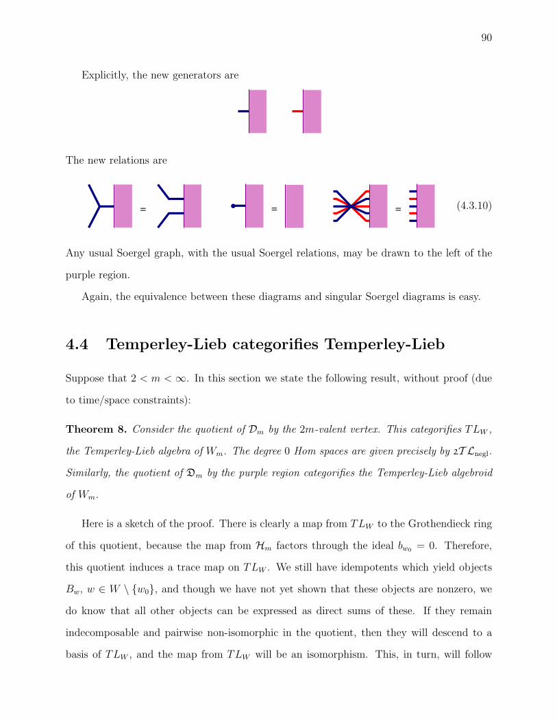
90

Explicitly, the new generators are

The new relations are

= = = (4.3.10)

Any usual Soergel graph, with the usual Soergel relations, may be drawn to the left of the

purple region.

Again, the equivalence between these diagrams and singular Soergel diagrams is easy.

4.4 Temperley-Lieb categorifies Temperley-Lieb

Suppose that 2 < m < ∞. In this section we state the following result, without proof (due

to time/space constraints):

Theorem 8. Consider the quotient of Dm by the 2m-valent vertex. This categorifies TLW ,

the Temperley-Lieb algebra of Wm. The degree 0 Hom spaces are given precisely by 2T Lnegl.

Similarly, the quotient of Dm by the purple region categorifies the Temperley-Lieb algebroid

of Wm.

Here is a sketch of the proof. There is clearly a map from TLW to the Grothendieck ring

of this quotient, because the map from Hm factors through the ideal bw0 = 0. Therefore,

this quotient induces a trace map on TLW . We still have idempotents which yield objects

Bw, w ∈ W \ {w0}, and though we have not yet shown that these objects are nonzero, we

do know that all other objects can be expressed as direct sums of these. If they remain

indecomposable and pairwise non-isomorphic in the quotient, then they will descend to a

basis of TLW , and the map from TLW will be an isomorphism. This, in turn, will follow

91

from the calculation of the trace on TLW , because the graded rank of End(Bw) will be in

1 + vZ[v], and the graded rank of Hom(Bw, Bx) for w 6= x will be in vZ[v].

In order to calculate the trace map, we must determine what elements of Hom(Bi , B∅)

survive in the quotient, for each reduced expression i . This is a diagrammatic calculation.

For instance, what will be End(B∅) in the quotient category? We rephrase this in singular

language: consider a Soergel 1-manifold diagram with a purple region and with empty white

boundary. We know that this reduces to a polynomial in R, but which polynomials can

appear? We claim that the polynomials which appear are precisely the ideal generated by

L, and that therefore End(B∅) ∼= R/L.

Let us excise a neighborhood of vm from our diagram: the remainder of the picture is

a Soergel diagram on the punctured plane whose boundary consists of 2m colored bands

entering the puncture. The first step will be to show that any diagram on the punctured

plane with that boundary which entirely wraps the puncture (so that it can’t be contained

in a simply-connected subregion) will reduce to a polynomial in this ideal. We know what

all the diagrams on the plane with that boundary reduce to: either ∞-diagrams or a single

2m-valent vertex. Two 2m-valent vertices which are connected by all 2m edges will be zero,

however, by Remark 4.2.7. The only ∞-diagram which can be placed safely next to a 2m-

valent vertex is generated over R by the all-dot, and the result is generated over R by L.

This calculation is done for the case m = 3 in [6].

Similarly, Hom(Bs, B∅) should be isomorphic to R/ L

fs{1}, where each polynomial is placed

next to the blue dot. This kernel is generated by the 2m-valent vertex with all but one dot

attached. Hom(Bs ⊗Bt, B∅) should be isomorphic to R/ L

fsft{2}, generated by a dot of each

color. However, Hom(Bs ⊗ Bt ⊗ Bs) has two generators, and one will need to be more

precise to describe the Hom spaces. Nonetheless, a simple diagrammatic argument should

still suffice to calculate this Hom space.

92

Bibliography

[1] D. Bar-Natan and S. Morrison, The Karoubi envelope and Lee’s degeneration of Kho-vanov homology, Algebr. Geom. Topol. 6 (2006), 1459–1469. arXiv:math/0606542.

[2] J. Barrett and B. Westbury, Spherical categories, Adv. Math. 143 (1999), 357–375.arXiv:hep-th/9310164v2.

[3] S. Bigelow, S. Morrison, E. Peters, and N. Snyder, Constructing the extended Haagerupplanar algebra, preprint 2009, arXiv:0909.4099.

[4] P. Das, S. Ghosh, and V. Gupta, Perturbations of planar algebras, preprint 2010,arXiv:1009.0186v2.

[5] B. Elias, A diagrammatic category for generalized Bott-Samelson bimodules and a dia-grammatic categorification of induced trivial modules for Hecke algebras, preprint 2010,arXiv:1009.2120.

[6] B. Elias, A diagrammatic Temperley-Lieb categorification, preprint 2010,arXiv:1003.3416. To appear in Intl. J. of Math. and Math. Sci..

[7] B. Elias and M. Khovanov, Diagrammatics for Soergel categories, preprint 2009,arXiv:0902.4700.

[8] B. Elias and G. Williamson, Diagrammatics for singular Soergel bimodules in type A,work in progress.

[9] B. Elias and G. Williamson, On cubes of Frobenius extensions, work in progress.

[10] I. Frenkel and M. Khovanov, Canonical bases in tensor products and graphical calculusfor Uq(sl2), Duke Math. J. 87 (1997), 409–480.

[11] F. Goodman and H. Wenzl, Ideals in the Temperley-Lieb category, appendix to: Amathematical model with a possible Chern-Simons phase by M. Freedman, Commun.Math. Phys. 234 (2003), 129–183.

[12] J.J. Graham and G.I. Lehrer, The representation theory of affine Temperley-Lieb alge-bras, Enseign. Math. 44 (1998), no. 3-4, 173218.

[13] J. Humphreys, Reflection groups and Coxeter groups, Cambridge University Press, 1992.

93

[14] V. F. R. Jones, The annular structure of subfactors, to appear in Enseign. Math.,arXiv:math/0105071v1.

[15] V. F. R. Jones, Index for subfactors, Invent. Math. 72 (1983), 1–25.

[16] V. F. R. Jones, Braid groups, Hecke algebras and type II 1 factors, from: Geomet-ric methods in operator algebras (Kyoto, 1983), Pitman Res. Notes Math. Ser. 123,Longman Sci. Tech., Harlow (1986), 242–273.

[17] L. Kauffman, State models and the Jones polynomial, Topology 26 (1987), 395–407.

[18] M. Khovanov and A. Lauda, A diagrammatic approach to categorification of quantumgroups I, Represent. Theory 13 (2009), 309–347. arXiv:0803.4121.

[19] A. Lauda, A categorification of quantum sl(2), Adv. in Math. 225 (2010), no. 6 , 3327–3424. arXiv:0803.3652.

[20] N. Libedinsky, Presentation of right-angled Soergel categories by generators and rela-tions, preprint 2008, arXiv:0810.2395.

[21] S. Morrison, A formula for the Jones-Wenzl projections , unpublished, available athttp://tqft.net/math/JonesWenzlProjections.pdf

[22] S. Morrison and N. Snyder, Non-cyclotomic fusion categories, preprint 2010,arXiv:1002.0168v2.

[23] W. Soergel, Category O, perverse sheaves and modules over the coinvariants for theWeyl group, J. Amer. Math. Soc. 3 (1990), no. 2, 421–445.

[24] W. Soergel, The combinatorics of Harish-Chandra bimodules, J. Reine Angew. Math.429 (1992), 49–74.

[25] W. Soergel, Gradings on representation categories, Proc. of the ICM (1995), 800–806.

[26] W. Soergel, Combinatorics of Harish-Chandra modules, in the book RepresentationTheories and Algebraic Geometry, edited by A. Broer, Kluwer (1998), pp. 401–412.

[27] W. Soergel, Kazhdan-Lusztig polynomials and indecomposable bimodules over polyno-mial rings, J. Inst. Math. Jussieu 6 (2007), no. 3, 501–525. English translation availableon Soergel’s webpage.

[28] H. Temperley and E. Lieb, Relations between the “percolation” and “colouring” problemand other graph-theoretical problems associated with regular planar lattices: some exactresults for the “percolation” problem, Proc. Roy. Soc. London Ser. A 322 (1971), 251–280.

[29] V. Turaev, Modular categories and 3-manifold invariants, Internat. J. Modern Phys. 6

(1992), 1807–1824.

94

[30] H. Wenzl, On sequences of projections, C. R. Math. Rep. Acad. Sci. Canada 9 (1987),no. 1, 59.

[31] G. Williamson, Singular Soergel Bimodules, PhD Thesis 2008, preprint 2010.arXiv:1010.1283v1.

Ben Elias, Department of Mathematics, Columbia University, New York, NY 10027

email: belias@math.columbia.edu