Embed Size (px)
Citation preview
Soft ComputingLecture Notes on Machine Learning
Matteo Mattecci
Department of Electronics and Information
Politecnico di Milano
Matteo Matteucci c©Lecture Notes on Machine Learning – p. 1/22
Supervised Learning– Bayes Classifiers –
Matteo Matteucci c©Lecture Notes on Machine Learning – p. 2/22
Maximum Likelihood vs. Maximum A Posteriory
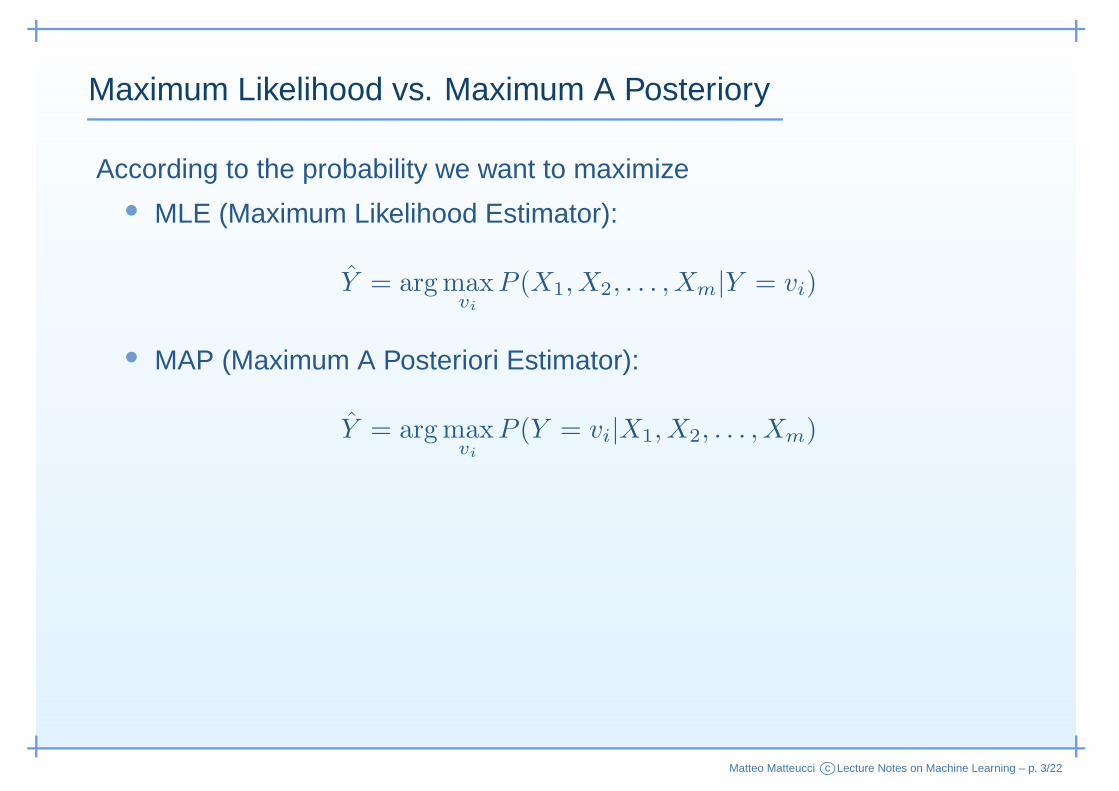
According to the probability we want to maximize• MLE (Maximum Likelihood Estimator):
Y = argmaxvi
P (X1, X2, . . . , Xm|Y = vi)
• MAP (Maximum A Posteriori Estimator):
Y = argmaxvi
P (Y = vi|X1, X2, . . . , Xm)
Matteo Matteucci c©Lecture Notes on Machine Learning – p. 3/22
Maximum Likelihood vs. Maximum A Posteriory
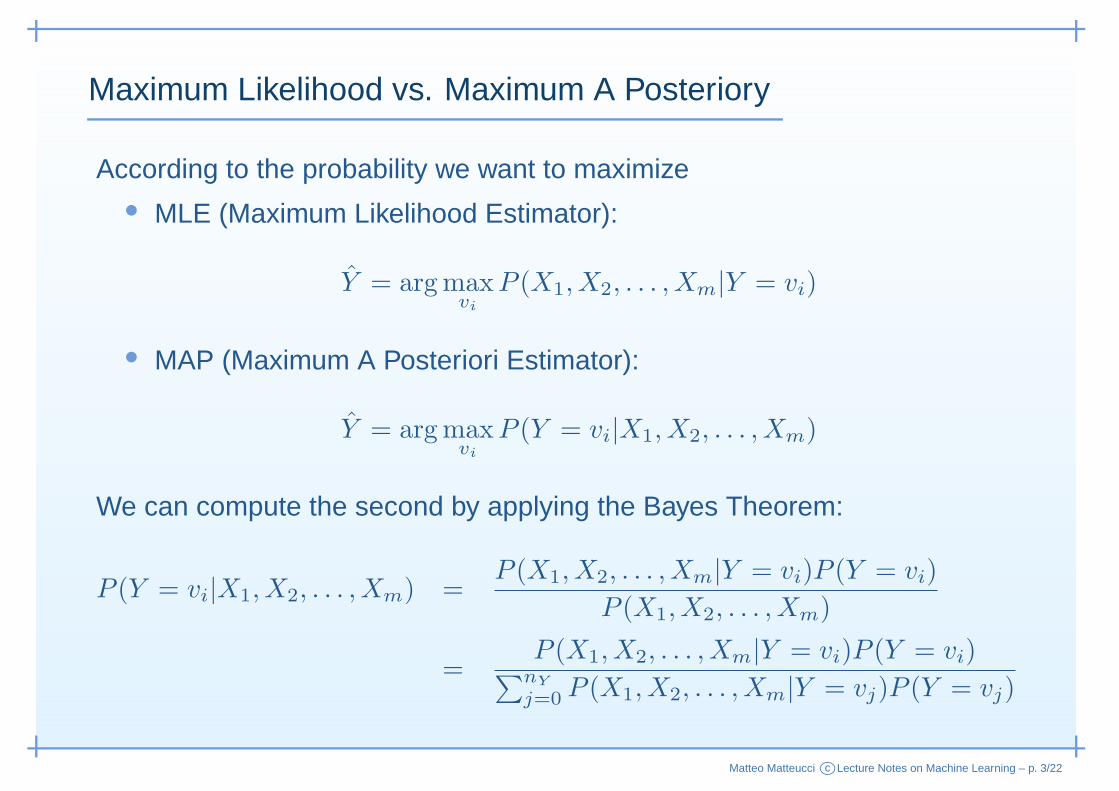
According to the probability we want to maximize• MLE (Maximum Likelihood Estimator):
Y = argmaxvi
P (X1, X2, . . . , Xm|Y = vi)
• MAP (Maximum A Posteriori Estimator):
Y = argmaxvi
P (Y = vi|X1, X2, . . . , Xm)
We can compute the second by applying the Bayes Theorem:
P (Y = vi|X1, X2, . . . , Xm) =P (X1, X2, . . . , Xm|Y = vi)P (Y = vi)
P (X1, X2, . . . , Xm)
=P (X1, X2, . . . , Xm|Y = vi)P (Y = vi)
∑nY
j=0 P (X1, X2, . . . , Xm|Y = vj)P (Y = vj)
Matteo Matteucci c©Lecture Notes on Machine Learning – p. 3/22
Bayes Classifiers Unleashed
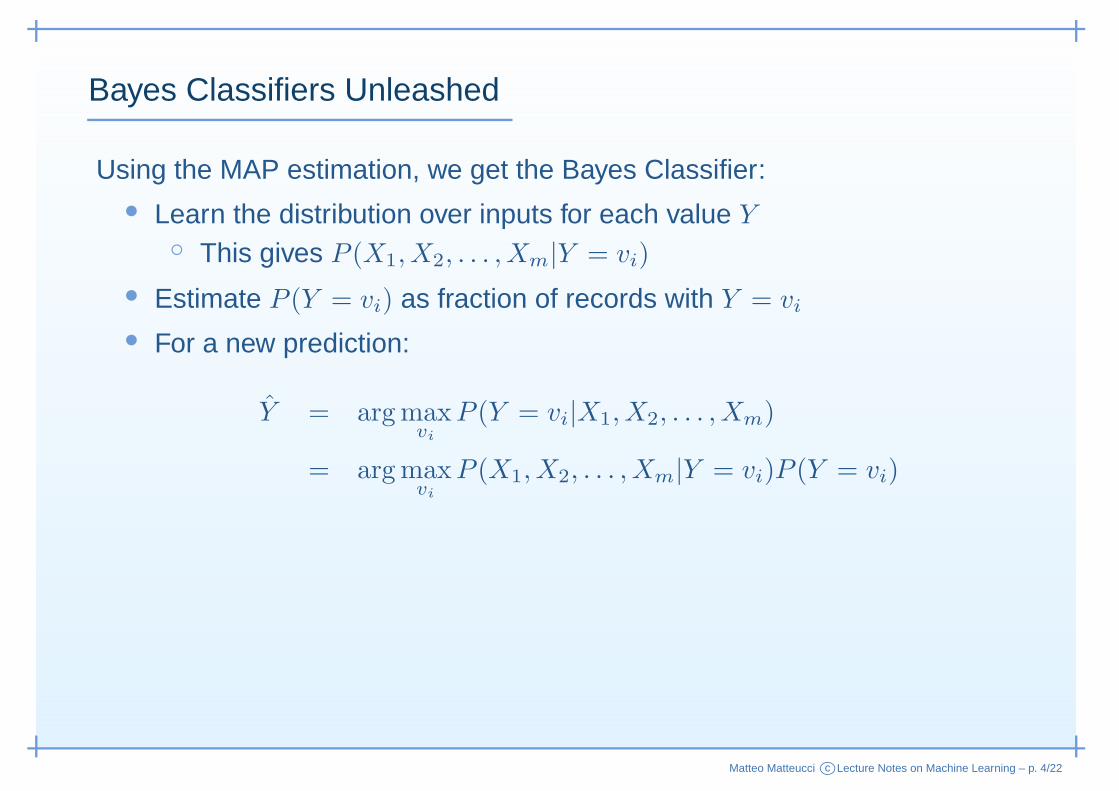
Using the MAP estimation, we get the Bayes Classifier:• Learn the distribution over inputs for each value Y
◦ This gives P (X1, X2, . . . , Xm|Y = vi)
• Estimate P (Y = vi) as fraction of records with Y = vi
• For a new prediction:
Y = argmaxvi
P (Y = vi|X1, X2, . . . , Xm)
= argmaxvi
P (X1, X2, . . . , Xm|Y = vi)P (Y = vi)
Matteo Matteucci c©Lecture Notes on Machine Learning – p. 4/22
Bayes Classifiers Unleashed
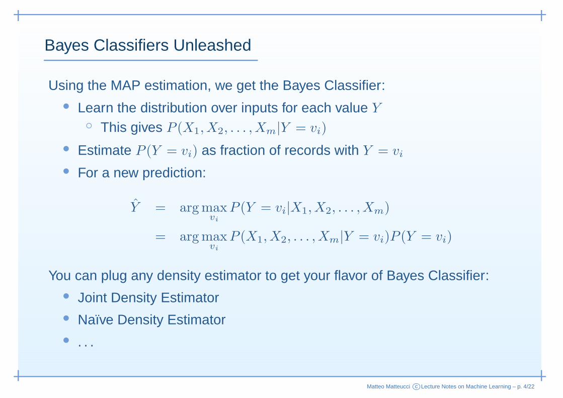
Using the MAP estimation, we get the Bayes Classifier:• Learn the distribution over inputs for each value Y
◦ This gives P (X1, X2, . . . , Xm|Y = vi)
• Estimate P (Y = vi) as fraction of records with Y = vi
• For a new prediction:
Y = argmaxvi
P (Y = vi|X1, X2, . . . , Xm)
= argmaxvi
P (X1, X2, . . . , Xm|Y = vi)P (Y = vi)
You can plug any density estimator to get your flavor of Bayes Classifier:• Joint Density Estimator• Naïve Density Estimator• . . .
Matteo Matteucci c©Lecture Notes on Machine Learning – p. 4/22
Unsupervised Learning– Density Estimation –
Matteo Matteucci c©Lecture Notes on Machine Learning – p. 5/22
The Joint Distribution
Given two random variables X and Y , the joint distribution of X and Y isthe distribution of X and Y together: P (X,Y ).
Matteo Matteucci c©Lecture Notes on Machine Learning – p. 6/22
The Joint Distribution
Given two random variables X and Y , the joint distribution of X and Y isthe distribution of X and Y together: P (X,Y ).
How to make a joint distribution of M variables:
1. Make a truth table listing all combination of values
2. For each combination state/compute how probable it is
3. Check that all probabilities sum up to 1
Matteo Matteucci c©Lecture Notes on Machine Learning – p. 6/22
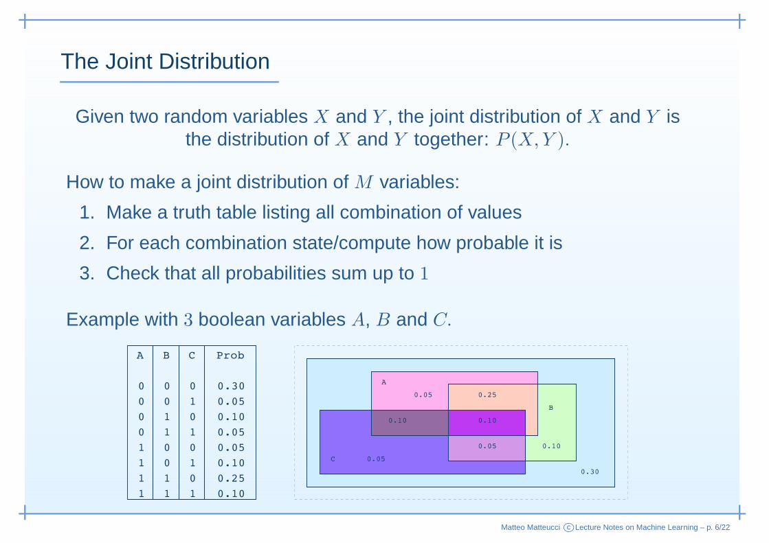
The Joint Distribution
Given two random variables X and Y , the joint distribution of X and Y isthe distribution of X and Y together: P (X,Y ).
How to make a joint distribution of M variables:
1. Make a truth table listing all combination of values
2. For each combination state/compute how probable it is
3. Check that all probabilities sum up to 1
Example with 3 boolean variables A, B and C.
Matteo Matteucci c©Lecture Notes on Machine Learning – p. 6/22
Using the Joint Distribution (I)
Compute probability for logic expression : P (E) =∑
Row∼E P (Row).
Matteo Matteucci c©Lecture Notes on Machine Learning – p. 7/22
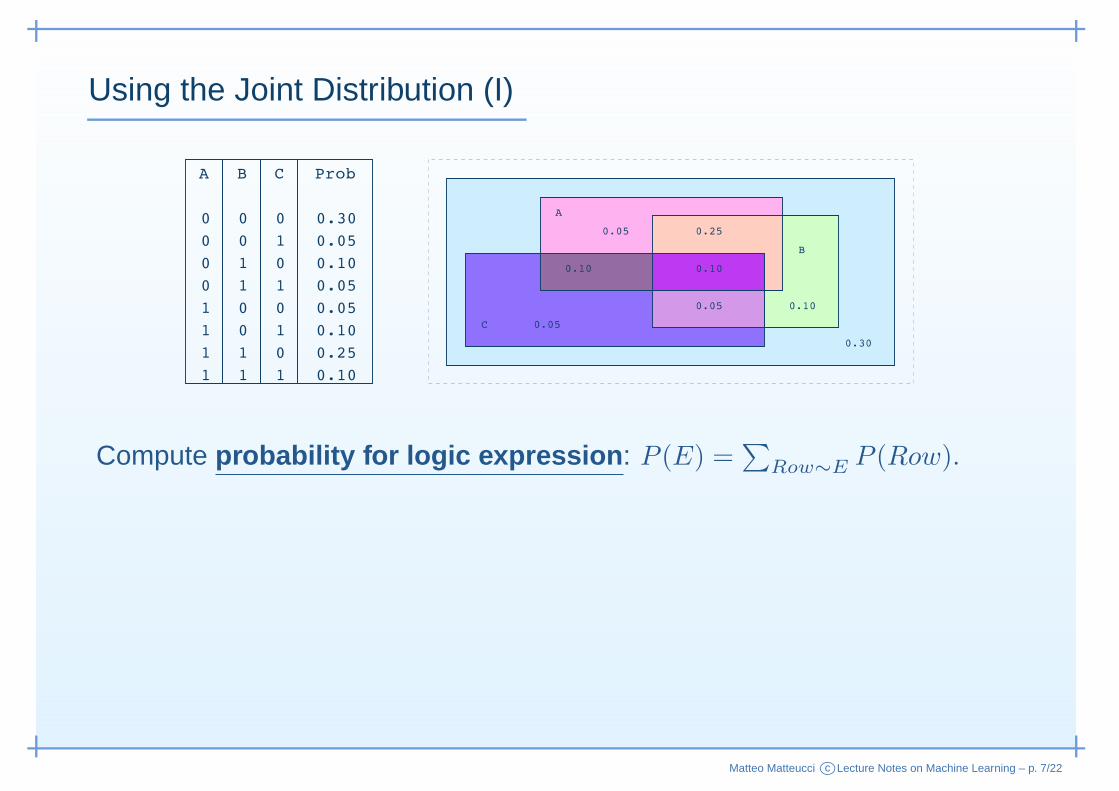
Using the Joint Distribution (I)
Compute probability for logic expression : P (E) =∑
Row∼E P (Row).
• P (A) = 0.05 + 0.10 + 0.25 + 0.10 = 0.5
• P (A ∧B) = 0.25 + 0.10 = 0.35
• P (A ∨ C) = 0.30 + 0.05 + 0.10 + 0.05 + 0.05 + 0.25 = 0.8
Matteo Matteucci c©Lecture Notes on Machine Learning – p. 7/22
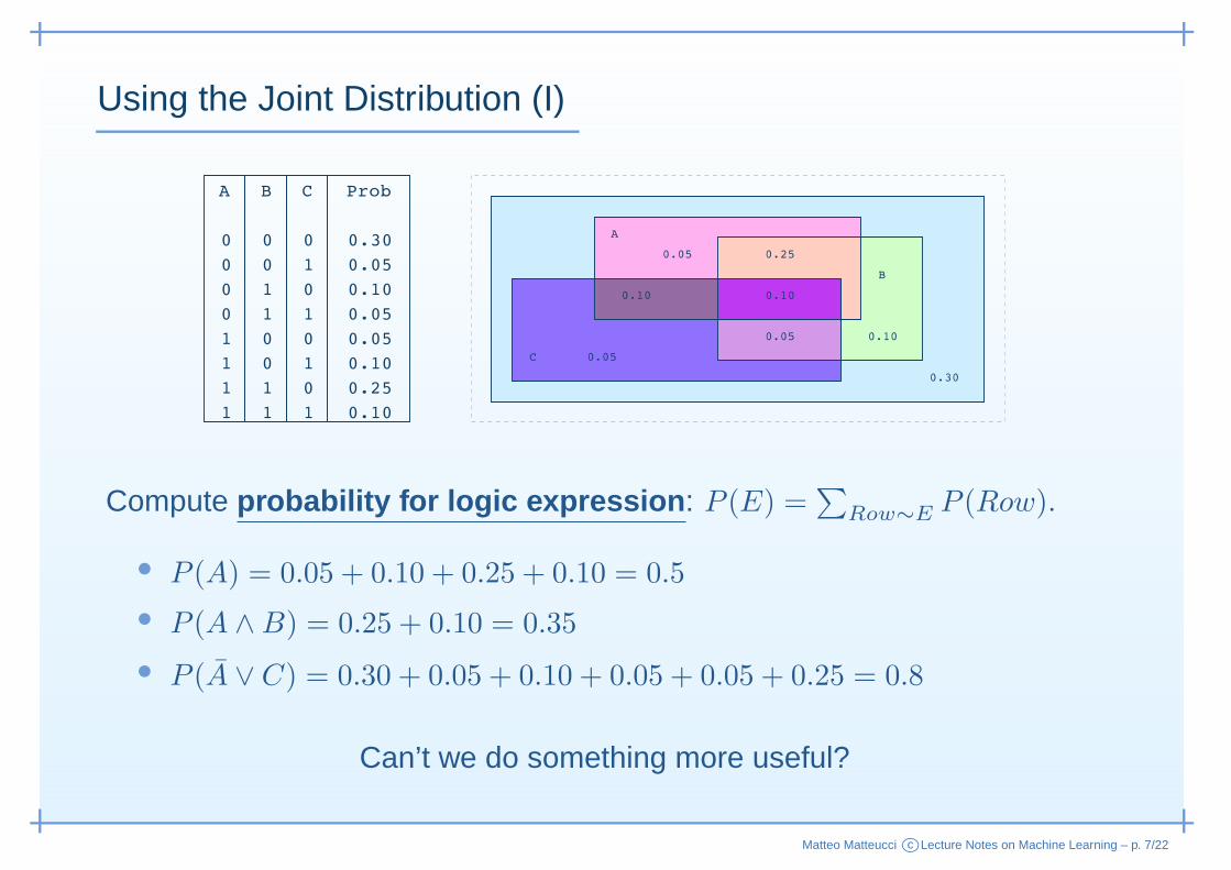
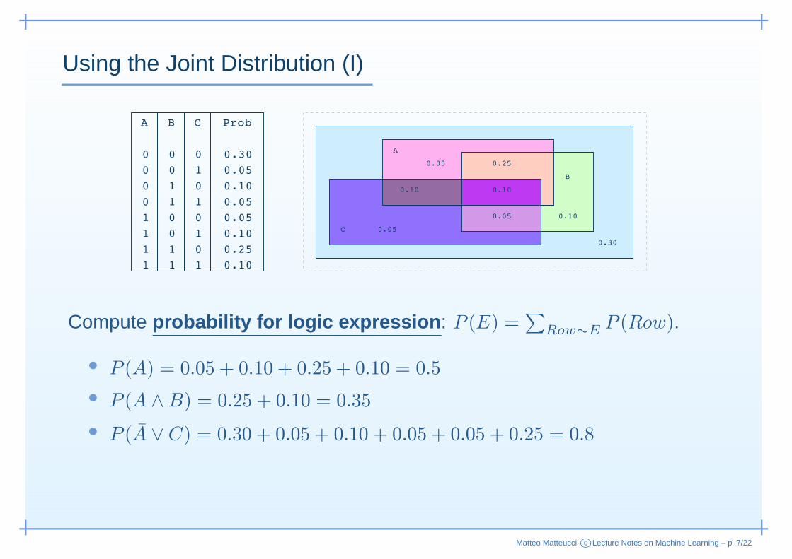
Using the Joint Distribution (I)
Compute probability for logic expression : P (E) =∑
Row∼E P (Row).
• P (A) = 0.05 + 0.10 + 0.25 + 0.10 = 0.5
• P (A ∧B) = 0.25 + 0.10 = 0.35
• P (A ∨ C) = 0.30 + 0.05 + 0.10 + 0.05 + 0.05 + 0.25 = 0.8
Can’t we do something more useful?
Matteo Matteucci c©Lecture Notes on Machine Learning – p. 7/22
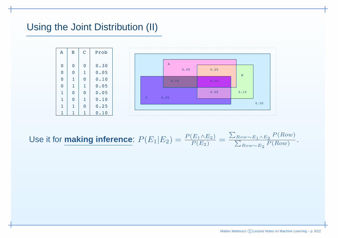
Using the Joint Distribution (II)
Use it for making inference : P (E1|E2) =P (E1∧E2)
P (E2)=
∑Row∼E1∧E2
P (Row)∑
Row∼E2P (Row) .
Matteo Matteucci c©Lecture Notes on Machine Learning – p. 8/22
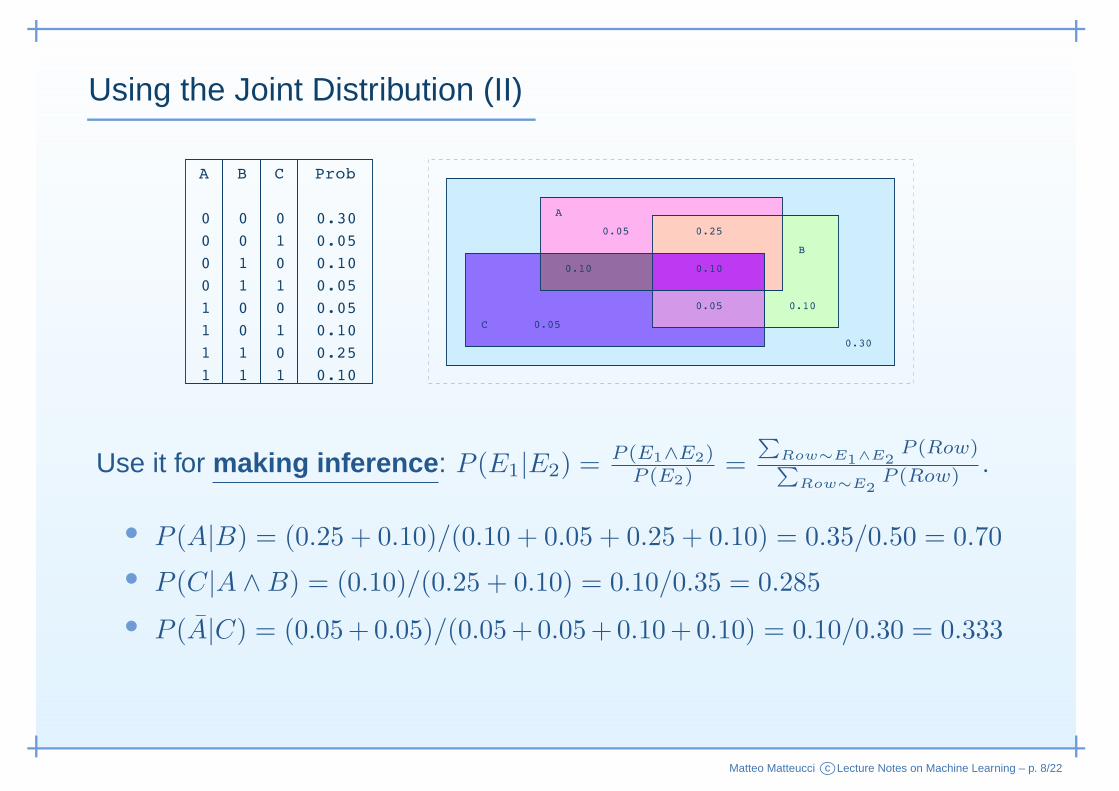
Using the Joint Distribution (II)
Use it for making inference : P (E1|E2) =P (E1∧E2)
P (E2)=
∑Row∼E1∧E2
P (Row)∑
Row∼E2P (Row) .
• P (A|B) = (0.25 + 0.10)/(0.10 + 0.05 + 0.25 + 0.10) = 0.35/0.50 = 0.70
• P (C|A ∧B) = (0.10)/(0.25 + 0.10) = 0.10/0.35 = 0.285
• P (A|C) = (0.05+0.05)/(0.05+0.05+0.10+0.10) = 0.10/0.30 = 0.333
Matteo Matteucci c©Lecture Notes on Machine Learning – p. 8/22
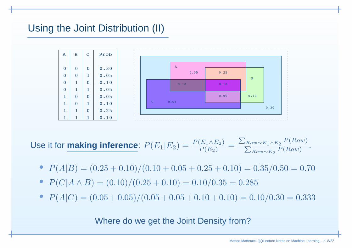
Using the Joint Distribution (II)
Use it for making inference : P (E1|E2) =P (E1∧E2)
P (E2)=
∑Row∼E1∧E2
P (Row)∑
Row∼E2P (Row) .
• P (A|B) = (0.25 + 0.10)/(0.10 + 0.05 + 0.25 + 0.10) = 0.35/0.50 = 0.70
• P (C|A ∧B) = (0.10)/(0.25 + 0.10) = 0.10/0.35 = 0.285
• P (A|C) = (0.05+0.05)/(0.05+0.05+0.10+0.10) = 0.10/0.30 = 0.333
Where do we get the Joint Density from?
Matteo Matteucci c©Lecture Notes on Machine Learning – p. 8/22
The Joint Distribution Estimator
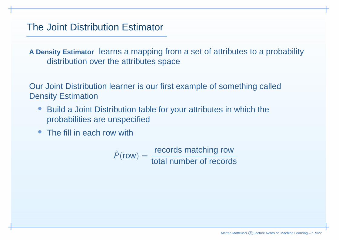
A Density Estimator learns a mapping from a set of attributes to a probabilitydistribution over the attributes space
Matteo Matteucci c©Lecture Notes on Machine Learning – p. 9/22
The Joint Distribution Estimator
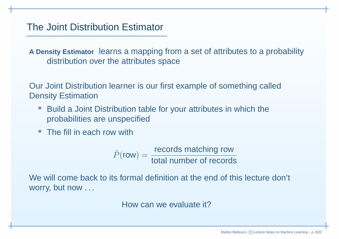
A Density Estimator learns a mapping from a set of attributes to a probabilitydistribution over the attributes space
Our Joint Distribution learner is our first example of something calledDensity Estimation
• Build a Joint Distribution table for your attributes in which theprobabilities are unspecified
• The fill in each row with
P (row) =records matching row
total number of records
Matteo Matteucci c©Lecture Notes on Machine Learning – p. 9/22
The Joint Distribution Estimator
A Density Estimator learns a mapping from a set of attributes to a probabilitydistribution over the attributes space
Our Joint Distribution learner is our first example of something calledDensity Estimation
• Build a Joint Distribution table for your attributes in which theprobabilities are unspecified
• The fill in each row with
P (row) =records matching row
total number of records
We will come back to its formal definition at the end of this lecture don’tworry, but now . . .
How can we evaluate it?
Matteo Matteucci c©Lecture Notes on Machine Learning – p. 9/22
Evaluating a Density Estimator
We can use likelihood for evaluating density estimation:• Given a record x, a density estimator M tells you how likely it is
P (x|M)
Matteo Matteucci c©Lecture Notes on Machine Learning – p. 10/22
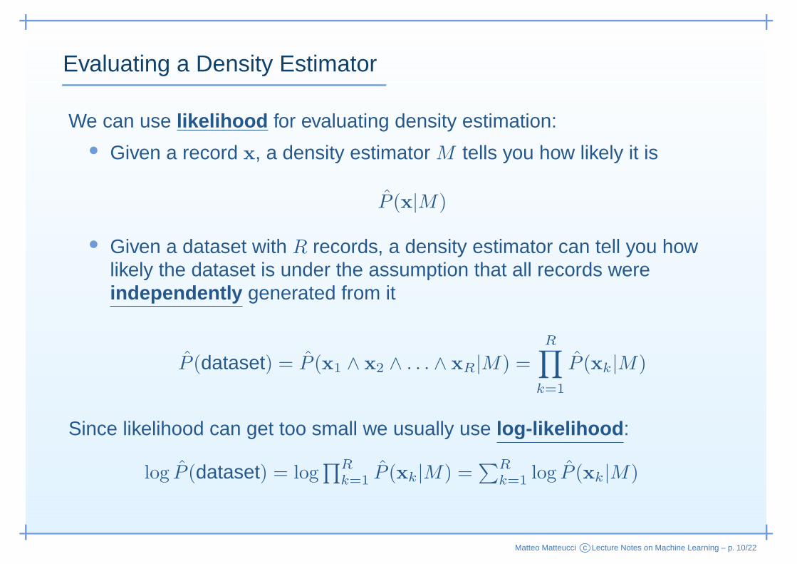
Evaluating a Density Estimator
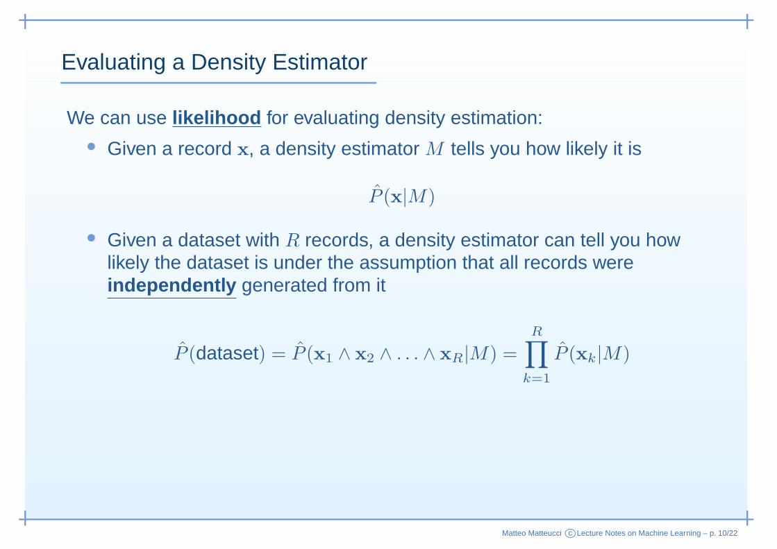
We can use likelihood for evaluating density estimation:• Given a record x, a density estimator M tells you how likely it is
P (x|M)
• Given a dataset with R records, a density estimator can tell you howlikely the dataset is under the assumption that all records wereindependently generated from it
P (dataset) = P (x1 ∧ x2 ∧ . . . ∧ xR|M) =
R∏
k=1
P (xk|M)
Matteo Matteucci c©Lecture Notes on Machine Learning – p. 10/22
Evaluating a Density Estimator
We can use likelihood for evaluating density estimation:• Given a record x, a density estimator M tells you how likely it is
P (x|M)
• Given a dataset with R records, a density estimator can tell you howlikely the dataset is under the assumption that all records wereindependently generated from it
P (dataset) = P (x1 ∧ x2 ∧ . . . ∧ xR|M) =
R∏
k=1
P (xk|M)
Since likelihood can get too small we usually use log-likelihood :
log P (dataset) = log∏R
k=1 P (xk|M) =∑R
k=1 log P (xk|M)
Matteo Matteucci c©Lecture Notes on Machine Learning – p. 10/22
Joint Distribution Summary
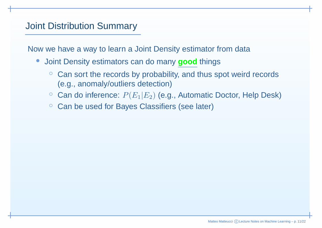
Now we have a way to learn a Joint Density estimator from data• Joint Density estimators can do many good things
◦ Can sort the records by probability, and thus spot weird records(e.g., anomaly/outliers detection)
◦ Can do inference: P (E1|E2) (e.g., Automatic Doctor, Help Desk)◦ Can be used for Bayes Classifiers (see later)
Matteo Matteucci c©Lecture Notes on Machine Learning – p. 11/22
Joint Distribution Summary
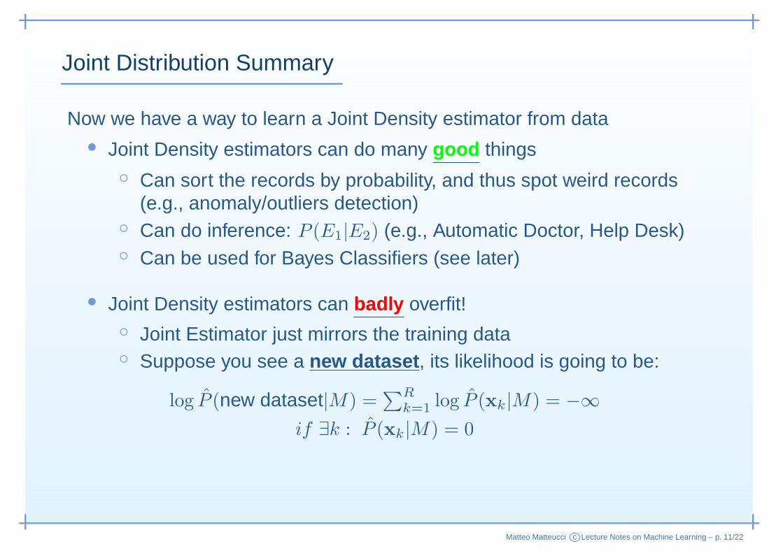
Now we have a way to learn a Joint Density estimator from data• Joint Density estimators can do many good things
◦ Can sort the records by probability, and thus spot weird records(e.g., anomaly/outliers detection)
◦ Can do inference: P (E1|E2) (e.g., Automatic Doctor, Help Desk)◦ Can be used for Bayes Classifiers (see later)
• Joint Density estimators can badly overfit!◦ Joint Estimator just mirrors the training data◦ Suppose you see a new dataset , its likelihood is going to be:
log P (new dataset|M) =∑R
k=1 log P (xk|M) = −∞
if ∃k : P (xk|M) = 0
Matteo Matteucci c©Lecture Notes on Machine Learning – p. 11/22
Joint Distribution Summary
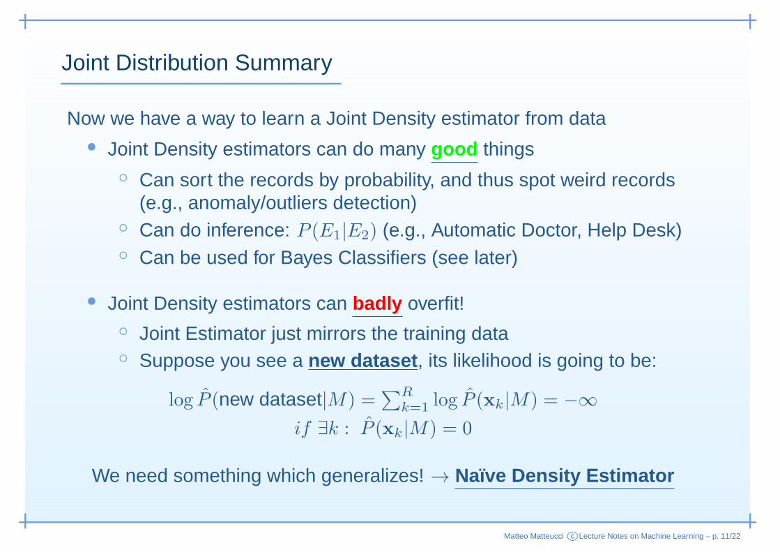
Now we have a way to learn a Joint Density estimator from data• Joint Density estimators can do many good things
◦ Can sort the records by probability, and thus spot weird records(e.g., anomaly/outliers detection)
◦ Can do inference: P (E1|E2) (e.g., Automatic Doctor, Help Desk)◦ Can be used for Bayes Classifiers (see later)
• Joint Density estimators can badly overfit!◦ Joint Estimator just mirrors the training data◦ Suppose you see a new dataset , its likelihood is going to be:
log P (new dataset|M) =∑R
k=1 log P (xk|M) = −∞
if ∃k : P (xk|M) = 0
We need something which generalizes! → Naïve Density Estimator
Matteo Matteucci c©Lecture Notes on Machine Learning – p. 11/22
Naıve Density Estimator
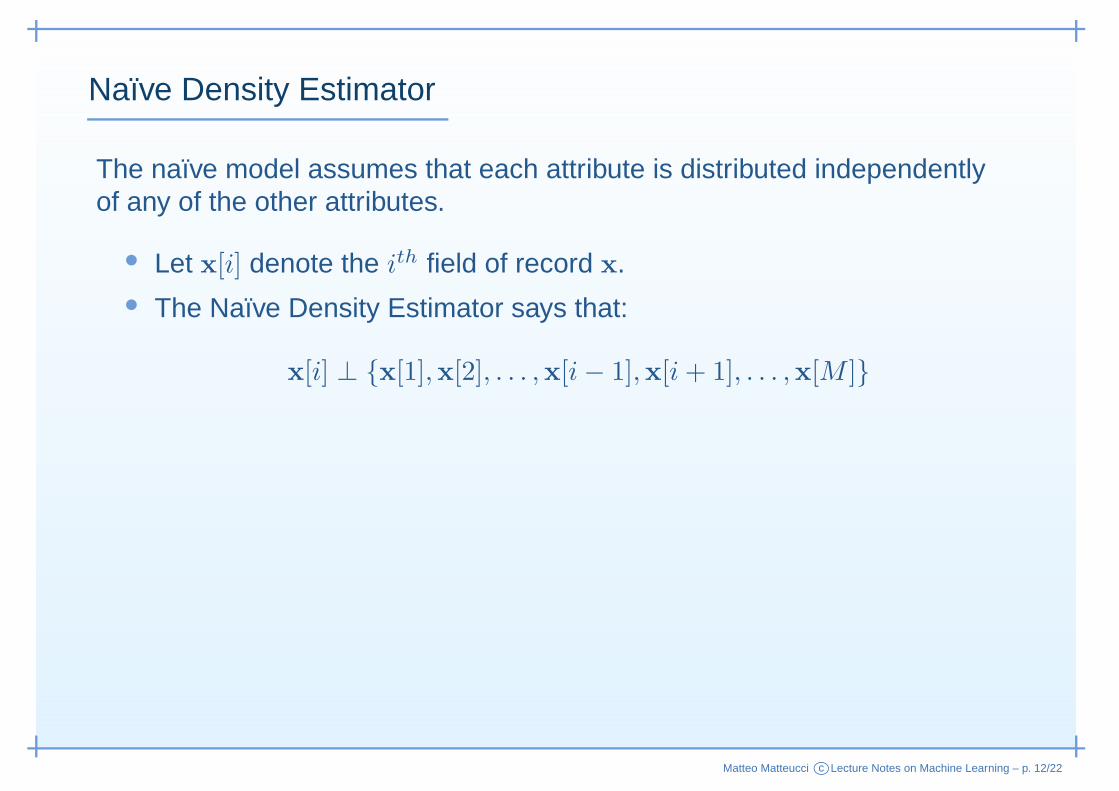
The naïve model assumes that each attribute is distributed independentlyof any of the other attributes.
• Let x[i] denote the ith field of record x.• The Naïve Density Estimator says that:
x[i] ⊥ {x[1],x[2], . . . ,x[i− 1],x[i+ 1], . . . ,x[M ]}
Matteo Matteucci c©Lecture Notes on Machine Learning – p. 12/22
Naıve Density Estimator
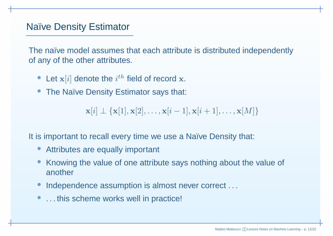
The naïve model assumes that each attribute is distributed independentlyof any of the other attributes.
• Let x[i] denote the ith field of record x.• The Naïve Density Estimator says that:
x[i] ⊥ {x[1],x[2], . . . ,x[i− 1],x[i+ 1], . . . ,x[M ]}
It is important to recall every time we use a Naïve Density that:• Attributes are equally important• Knowing the value of one attribute says nothing about the value of
another• Independence assumption is almost never correct . . .• . . . this scheme works well in practice!
Matteo Matteucci c©Lecture Notes on Machine Learning – p. 12/22
Naıve Density Estimator: An Example
From a Naïve Distribution you can compute the Joint Distribution:
• Suppose A,B,C,D independently distributed, P (A ∧ B ∧ C ∧ D) =?
Matteo Matteucci c©Lecture Notes on Machine Learning – p. 13/22
Naıve Density Estimator: An Example
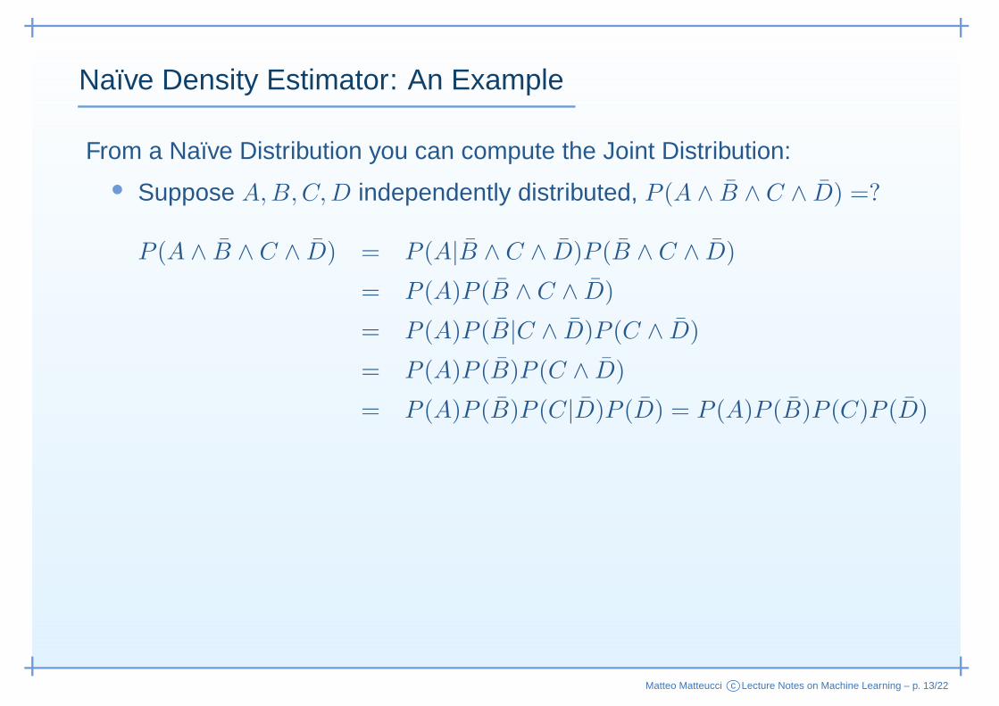
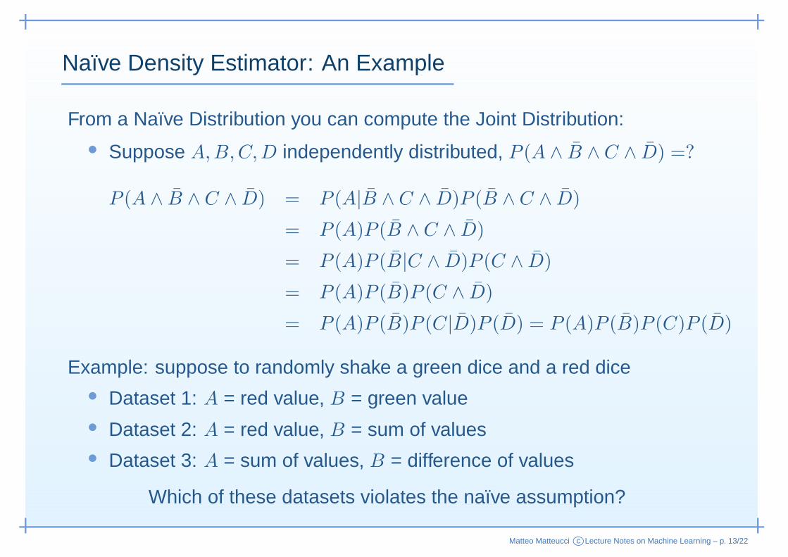
From a Naïve Distribution you can compute the Joint Distribution:
• Suppose A,B,C,D independently distributed, P (A ∧ B ∧ C ∧ D) =?
P (A ∧ B ∧ C ∧ D) = P (A|B ∧ C ∧ D)P (B ∧ C ∧ D)
= P (A)P (B ∧ C ∧ D)
= P (A)P (B|C ∧ D)P (C ∧ D)
= P (A)P (B)P (C ∧ D)
= P (A)P (B)P (C|D)P (D) = P (A)P (B)P (C)P (D)
Matteo Matteucci c©Lecture Notes on Machine Learning – p. 13/22
Naıve Density Estimator: An Example
From a Naïve Distribution you can compute the Joint Distribution:
• Suppose A,B,C,D independently distributed, P (A ∧ B ∧ C ∧ D) =?
P (A ∧ B ∧ C ∧ D) = P (A|B ∧ C ∧ D)P (B ∧ C ∧ D)
= P (A)P (B ∧ C ∧ D)
= P (A)P (B|C ∧ D)P (C ∧ D)
= P (A)P (B)P (C ∧ D)
= P (A)P (B)P (C|D)P (D) = P (A)P (B)P (C)P (D)
Example: suppose to randomly shake a green dice and a red dice• Dataset 1: A = red value, B = green value• Dataset 2: A = red value, B = sum of values• Dataset 3: A = sum of values, B = difference of values
Which of these datasets violates the naïve assumption?
Matteo Matteucci c©Lecture Notes on Machine Learning – p. 13/22
Learning a Naıve Density Estimator
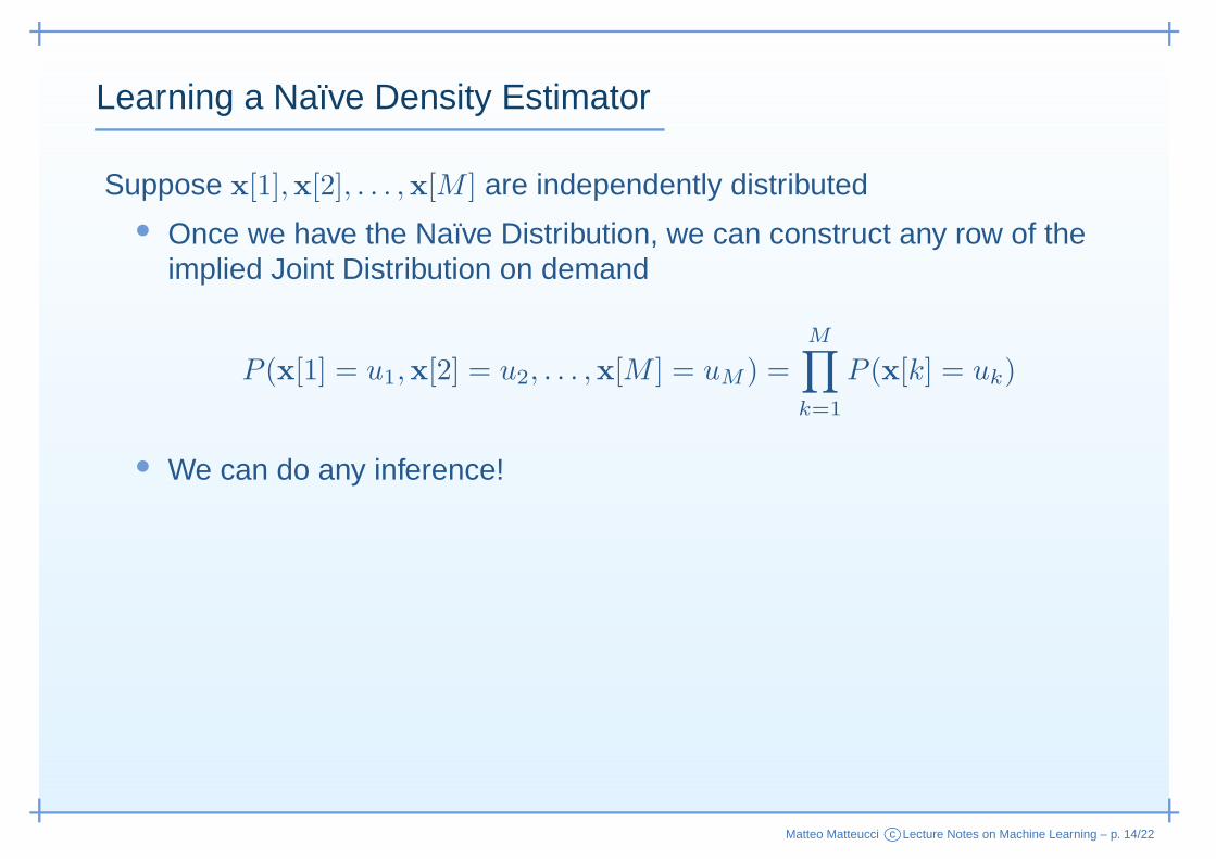
Suppose x[1],x[2], . . . ,x[M ] are independently distributed
• Once we have the Naïve Distribution, we can construct any row of theimplied Joint Distribution on demand
P (x[1] = u1,x[2] = u2, . . . ,x[M ] = uM ) =
M∏
k=1
P (x[k] = uk)
• We can do any inference!
Matteo Matteucci c©Lecture Notes on Machine Learning – p. 14/22
Learning a Naıve Density Estimator
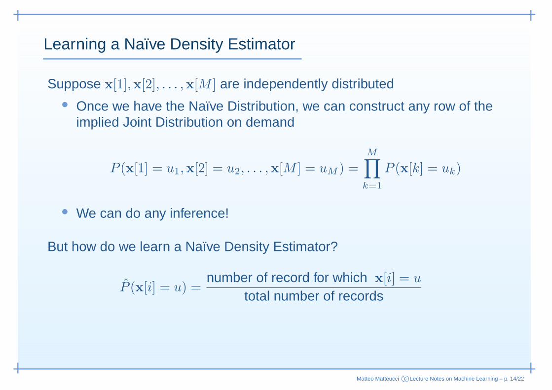
Suppose x[1],x[2], . . . ,x[M ] are independently distributed
• Once we have the Naïve Distribution, we can construct any row of theimplied Joint Distribution on demand
P (x[1] = u1,x[2] = u2, . . . ,x[M ] = uM ) =
M∏
k=1
P (x[k] = uk)
• We can do any inference!
But how do we learn a Naïve Density Estimator?
P (x[i] = u) =number of record for which x[i] = u
total number of records
Matteo Matteucci c©Lecture Notes on Machine Learning – p. 14/22
Learning a Naıve Density Estimator
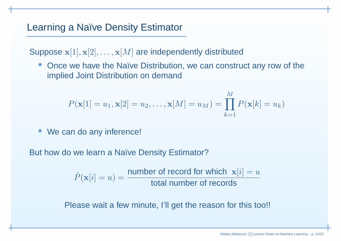
Suppose x[1],x[2], . . . ,x[M ] are independently distributed
• Once we have the Naïve Distribution, we can construct any row of theimplied Joint Distribution on demand
P (x[1] = u1,x[2] = u2, . . . ,x[M ] = uM ) =
M∏
k=1
P (x[k] = uk)
• We can do any inference!
But how do we learn a Naïve Density Estimator?
P (x[i] = u) =number of record for which x[i] = u
total number of records
Please wait a few minute, I’ll get the reason for this too!!
Matteo Matteucci c©Lecture Notes on Machine Learning – p. 14/22
Joint Density vs. Naıve Density
What we got so far? Let’s try to summarize things up:• Joint Distribution Estimator
◦ Can model anything◦ Given 100 records and more than 6 Boolean attributes will
perform poorly◦ Can easily overfit the data
Matteo Matteucci c©Lecture Notes on Machine Learning – p. 15/22
Joint Density vs. Naıve Density
What we got so far? Let’s try to summarize things up:• Joint Distribution Estimator
◦ Can model anything◦ Given 100 records and more than 6 Boolean attributes will
perform poorly◦ Can easily overfit the data
• Naïve Distribution Estimator◦ Can model only very boring distributions◦ Given 100 records and 10,000 multivalued attributes will be fine◦ Quite robust to overfitting
So far we have two simple density estimators, in other lectures we’ll seevastly more impressive ones (Mixture Models, Bayesian Networks, . . . ).
But first, why should we care about density estimation?
Matteo Matteucci c©Lecture Notes on Machine Learning – p. 15/22
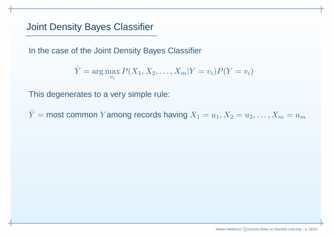
Joint Density Bayes Classifier
In the case of the Joint Density Bayes Classifier
Y = argmaxvi
P (X1, X2, . . . , Xm|Y = vi)P (Y = vi)
This degenerates to a very simple rule:
Y = most common Y among records having X1 = u1, X2 = u2, . . . , Xm = um
Matteo Matteucci c©Lecture Notes on Machine Learning – p. 16/22
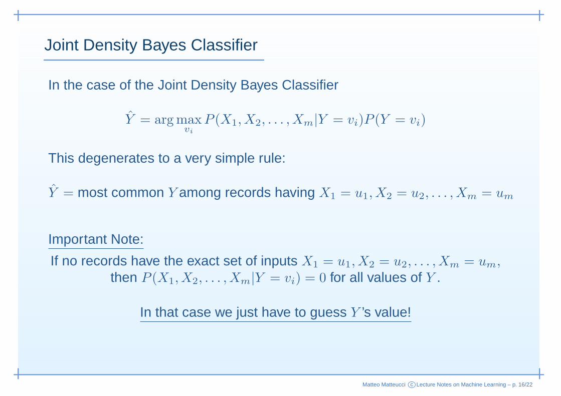
Joint Density Bayes Classifier
In the case of the Joint Density Bayes Classifier
Y = argmaxvi
P (X1, X2, . . . , Xm|Y = vi)P (Y = vi)
This degenerates to a very simple rule:
Y = most common Y among records having X1 = u1, X2 = u2, . . . , Xm = um
Important Note:
If no records have the exact set of inputs X1 = u1, X2 = u2, . . . , Xm = um,then P (X1, X2, . . . , Xm|Y = vi) = 0 for all values of Y .
In that case we just have to guess Y ’s value!
Matteo Matteucci c©Lecture Notes on Machine Learning – p. 16/22
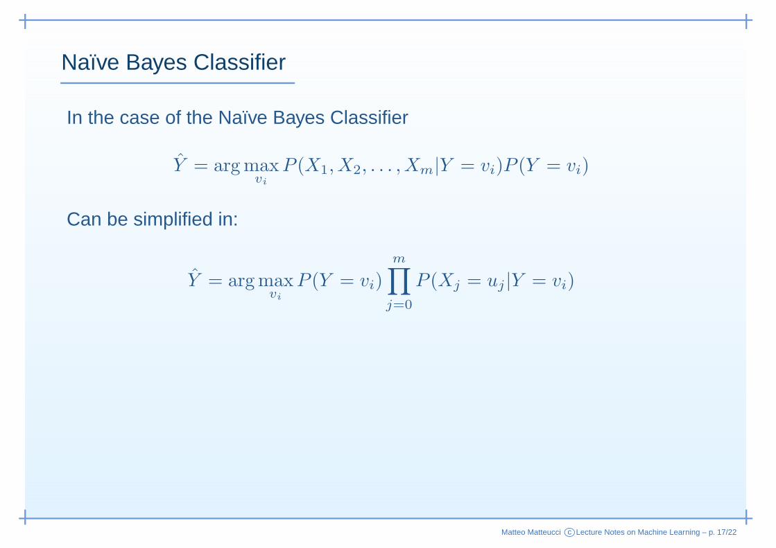
Naıve Bayes Classifier
In the case of the Naïve Bayes Classifier
Y = argmaxvi
P (X1, X2, . . . , Xm|Y = vi)P (Y = vi)
Can be simplified in:
Y = argmaxvi
P (Y = vi)
m∏
j=0
P (Xj = uj |Y = vi)
Matteo Matteucci c©Lecture Notes on Machine Learning – p. 17/22
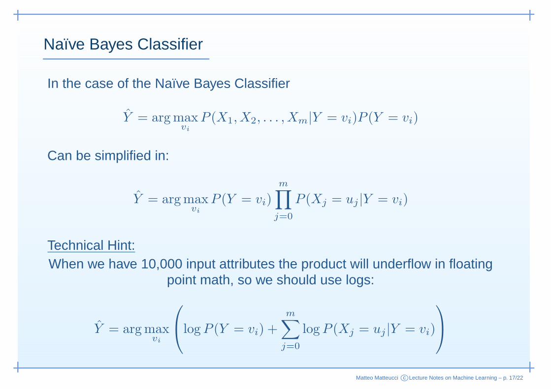
Naıve Bayes Classifier
In the case of the Naïve Bayes Classifier
Y = argmaxvi
P (X1, X2, . . . , Xm|Y = vi)P (Y = vi)
Can be simplified in:
Y = argmaxvi
P (Y = vi)
m∏
j=0
P (Xj = uj |Y = vi)
Technical Hint:When we have 10,000 input attributes the product will underflow in floating
point math, so we should use logs:
Y = argmaxvi
logP (Y = vi) +
m∑
j=0
logP (Xj = uj |Y = vi)
Matteo Matteucci c©Lecture Notes on Machine Learning – p. 17/22
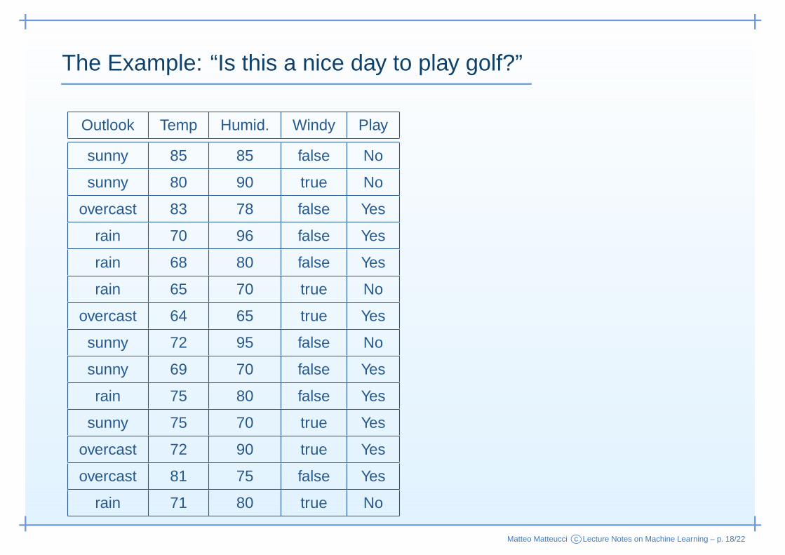
The Example: “Is this a nice day to play golf?”
Outlook Temp Humid. Windy Play
sunny 85 85 false No
sunny 80 90 true No
overcast 83 78 false Yes
rain 70 96 false Yes
rain 68 80 false Yes
rain 65 70 true No
overcast 64 65 true Yes
sunny 72 95 false No
sunny 69 70 false Yes
rain 75 80 false Yes
sunny 75 70 true Yes
overcast 72 90 true Yes
overcast 81 75 false Yes
rain 71 80 true No
Matteo Matteucci c©Lecture Notes on Machine Learning – p. 18/22
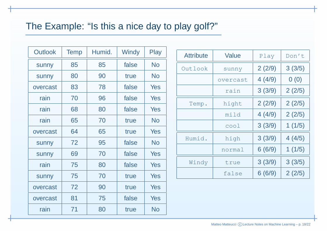
The Example: “Is this a nice day to play golf?”
Outlook Temp Humid. Windy Play
sunny 85 85 false No
sunny 80 90 true No
overcast 83 78 false Yes
rain 70 96 false Yes
rain 68 80 false Yes
rain 65 70 true No
overcast 64 65 true Yes
sunny 72 95 false No
sunny 69 70 false Yes
rain 75 80 false Yes
sunny 75 70 true Yes
overcast 72 90 true Yes
overcast 81 75 false Yes
rain 71 80 true No
Attribute Value Play Don’t
Outlook sunny 2 (2/9) 3 (3/5)
overcast 4 (4/9) 0 (0)
rain 3 (3/9) 2 (2/5)
Temp. hight 2 (2/9) 2 (2/5)
mild 4 (4/9) 2 (2/5)
cool 3 (3/9) 1 (1/5)
Humid. high 3 (3/9) 4 (4/5)
normal 6 (6/9) 1 (1/5)
Windy true 3 (3/9) 3 (3/5)
false 6 (6/9) 2 (2/5)
Matteo Matteucci c©Lecture Notes on Machine Learning – p. 18/22
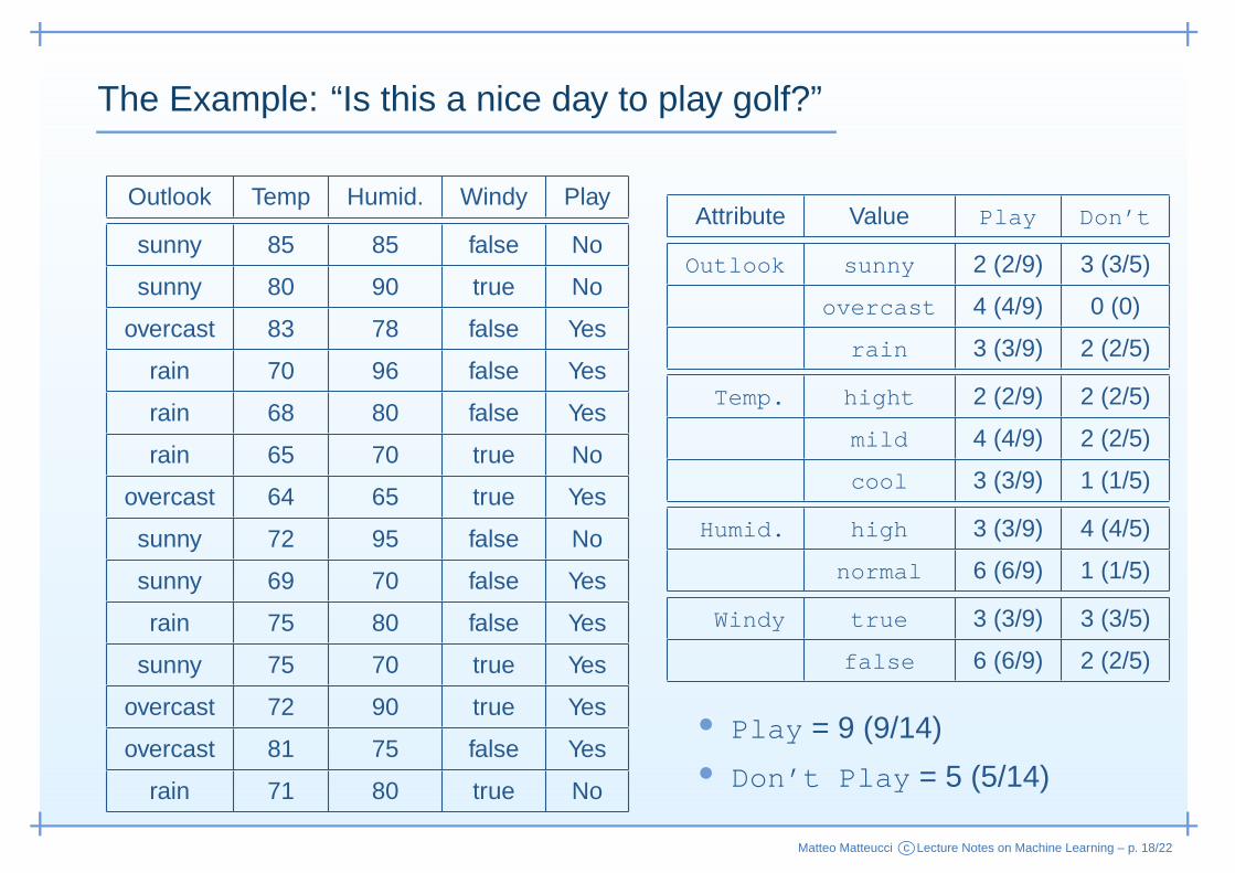
The Example: “Is this a nice day to play golf?”
Outlook Temp Humid. Windy Play
sunny 85 85 false No
sunny 80 90 true No
overcast 83 78 false Yes
rain 70 96 false Yes
rain 68 80 false Yes
rain 65 70 true No
overcast 64 65 true Yes
sunny 72 95 false No
sunny 69 70 false Yes
rain 75 80 false Yes
sunny 75 70 true Yes
overcast 72 90 true Yes
overcast 81 75 false Yes
rain 71 80 true No
Attribute Value Play Don’t
Outlook sunny 2 (2/9) 3 (3/5)
overcast 4 (4/9) 0 (0)
rain 3 (3/9) 2 (2/5)
Temp. hight 2 (2/9) 2 (2/5)
mild 4 (4/9) 2 (2/5)
cool 3 (3/9) 1 (1/5)
Humid. high 3 (3/9) 4 (4/5)
normal 6 (6/9) 1 (1/5)
Windy true 3 (3/9) 3 (3/5)
false 6 (6/9) 2 (2/5)
• Play = 9 (9/14)• Don’t Play = 5 (5/14)
Matteo Matteucci c©Lecture Notes on Machine Learning – p. 18/22
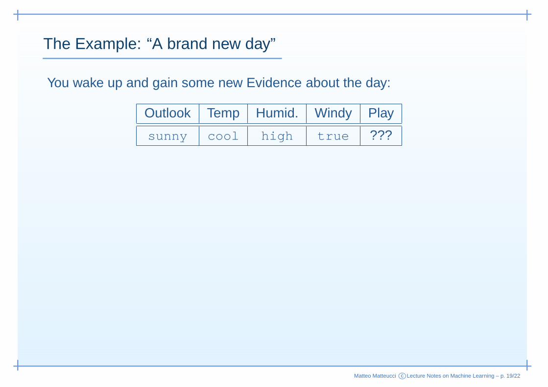
The Example: “A brand new day”
You wake up and gain some new Evidence about the day:
Outlook Temp Humid. Windy Play
sunny cool high true ???
Matteo Matteucci c©Lecture Notes on Machine Learning – p. 19/22
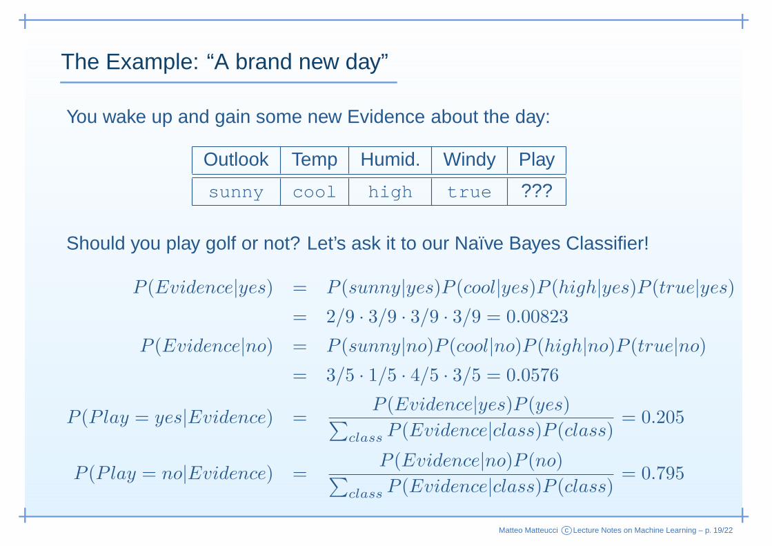
The Example: “A brand new day”
You wake up and gain some new Evidence about the day:
Outlook Temp Humid. Windy Play
sunny cool high true ???
Should you play golf or not? Let’s ask it to our Naïve Bayes Classifier!
P (Evidence|yes) = P (sunny|yes)P (cool|yes)P (high|yes)P (true|yes)
= 2/9 · 3/9 · 3/9 · 3/9 = 0.00823
P (Evidence|no) = P (sunny|no)P (cool|no)P (high|no)P (true|no)
= 3/5 · 1/5 · 4/5 · 3/5 = 0.0576
P (Play = yes|Evidence) =P (Evidence|yes)P (yes)
∑
class P (Evidence|class)P (class)= 0.205
P (Play = no|Evidence) =P (Evidence|no)P (no)
∑
class P (Evidence|class)P (class)= 0.795
Matteo Matteucci c©Lecture Notes on Machine Learning – p. 19/22
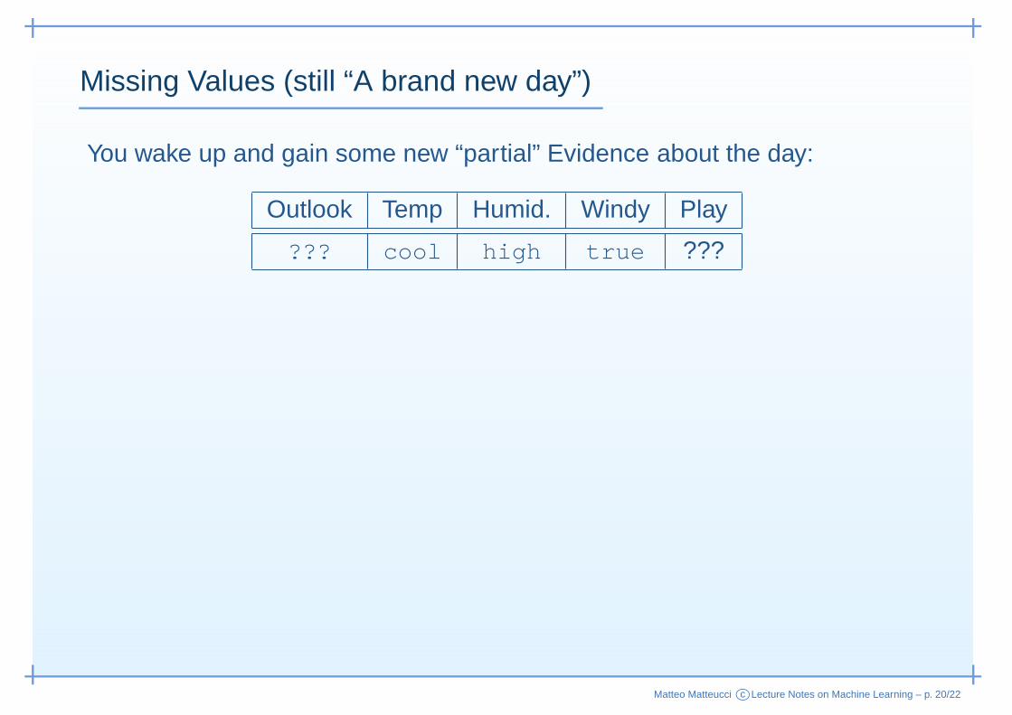
Missing Values (still “A brand new day”)
You wake up and gain some new “partial” Evidence about the day:
Outlook Temp Humid. Windy Play
??? cool high true ???
Matteo Matteucci c©Lecture Notes on Machine Learning – p. 20/22
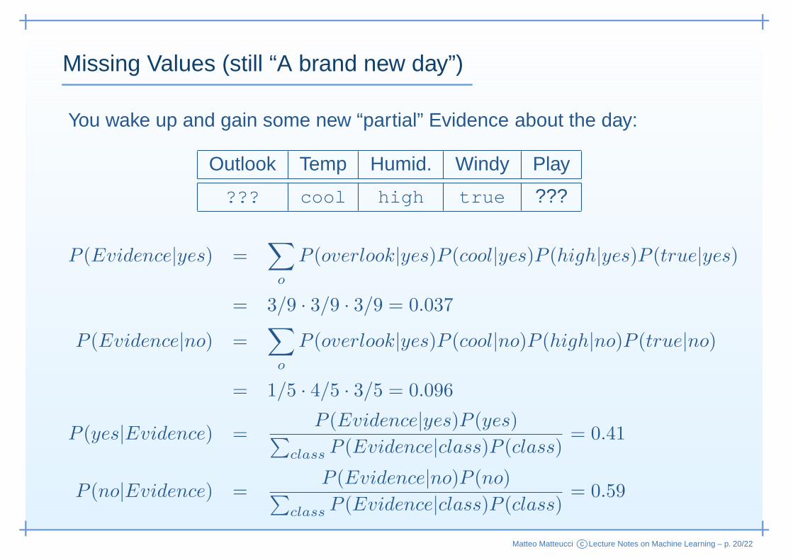
Missing Values (still “A brand new day”)
You wake up and gain some new “partial” Evidence about the day:
Outlook Temp Humid. Windy Play
??? cool high true ???
P (Evidence|yes) =∑
o
P (overlook|yes)P (cool|yes)P (high|yes)P (true|yes)
= 3/9 · 3/9 · 3/9 = 0.037
P (Evidence|no) =∑
o
P (overlook|yes)P (cool|no)P (high|no)P (true|no)
= 1/5 · 4/5 · 3/5 = 0.096
P (yes|Evidence) =P (Evidence|yes)P (yes)
∑
class P (Evidence|class)P (class)= 0.41
P (no|Evidence) =P (Evidence|no)P (no)
∑
class P (Evidence|class)P (class)= 0.59
Matteo Matteucci c©Lecture Notes on Machine Learning – p. 20/22
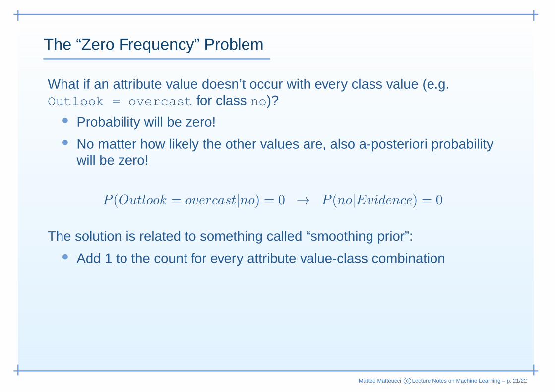
The “Zero Frequency” Problem
What if an attribute value doesn’t occur with every class value (e.g.Outlook = overcast for class no)?
• Probability will be zero!• No matter how likely the other values are, also a-posteriori probability
will be zero!
P (Outlook = overcast|no) = 0 → P (no|Evidence) = 0
Matteo Matteucci c©Lecture Notes on Machine Learning – p. 21/22
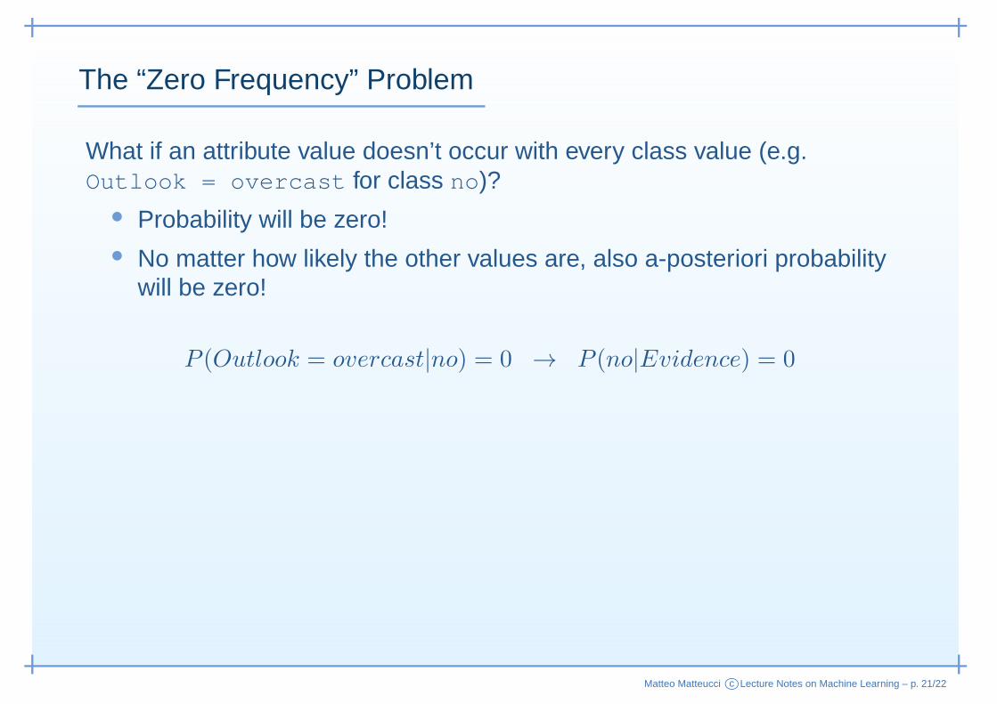
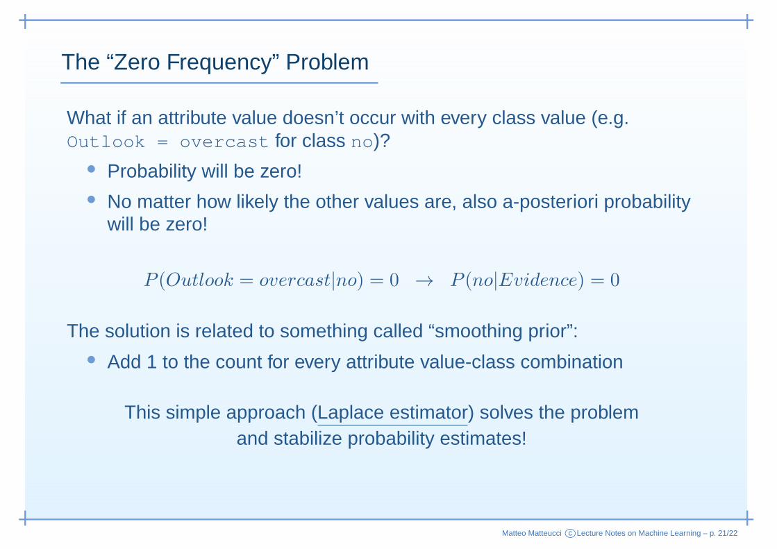
The “Zero Frequency” Problem
What if an attribute value doesn’t occur with every class value (e.g.Outlook = overcast for class no)?
• Probability will be zero!• No matter how likely the other values are, also a-posteriori probability
will be zero!
P (Outlook = overcast|no) = 0 → P (no|Evidence) = 0
The solution is related to something called “smoothing prior”:• Add 1 to the count for every attribute value-class combination
Matteo Matteucci c©Lecture Notes on Machine Learning – p. 21/22
The “Zero Frequency” Problem
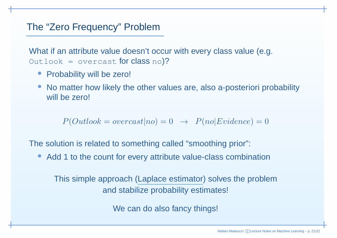
What if an attribute value doesn’t occur with every class value (e.g.Outlook = overcast for class no)?
• Probability will be zero!• No matter how likely the other values are, also a-posteriori probability
will be zero!
P (Outlook = overcast|no) = 0 → P (no|Evidence) = 0
The solution is related to something called “smoothing prior”:• Add 1 to the count for every attribute value-class combination
This simple approach (Laplace estimator) solves the problemand stabilize probability estimates!
Matteo Matteucci c©Lecture Notes on Machine Learning – p. 21/22
The “Zero Frequency” Problem
What if an attribute value doesn’t occur with every class value (e.g.Outlook = overcast for class no)?
• Probability will be zero!• No matter how likely the other values are, also a-posteriori probability
will be zero!
P (Outlook = overcast|no) = 0 → P (no|Evidence) = 0
The solution is related to something called “smoothing prior”:• Add 1 to the count for every attribute value-class combination
This simple approach (Laplace estimator) solves the problemand stabilize probability estimates!
We can do also fancy things!
Matteo Matteucci c©Lecture Notes on Machine Learning – p. 21/22
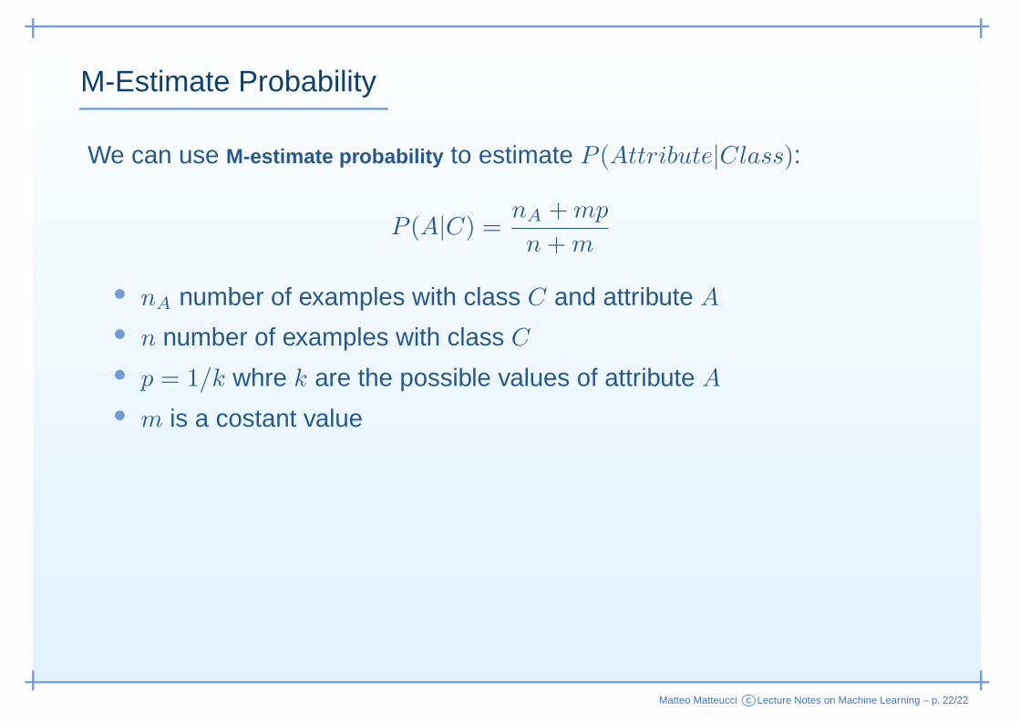
M-Estimate Probability
We can use M-estimate probability to estimate P (Attribute|Class):
P (A|C) =nA +mp
n+m
• nA number of examples with class C and attribute A
• n number of examples with class C
• p = 1/k whre k are the possible values of attribute A
• m is a costant value
Matteo Matteucci c©Lecture Notes on Machine Learning – p. 22/22
M-Estimate Probability
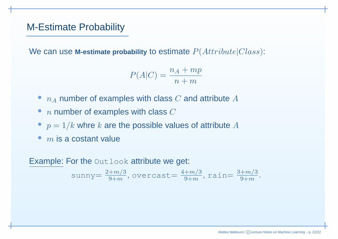
We can use M-estimate probability to estimate P (Attribute|Class):
P (A|C) =nA +mp
n+m
• nA number of examples with class C and attribute A
• n number of examples with class C
• p = 1/k whre k are the possible values of attribute A
• m is a costant value
Example: For the Outlook attribute we get:
sunny= 2+m/39+m , overcast= 4+m/3
9+m , rain= 3+m/39+m .
Matteo Matteucci c©Lecture Notes on Machine Learning – p. 22/22
M-Estimate Probability
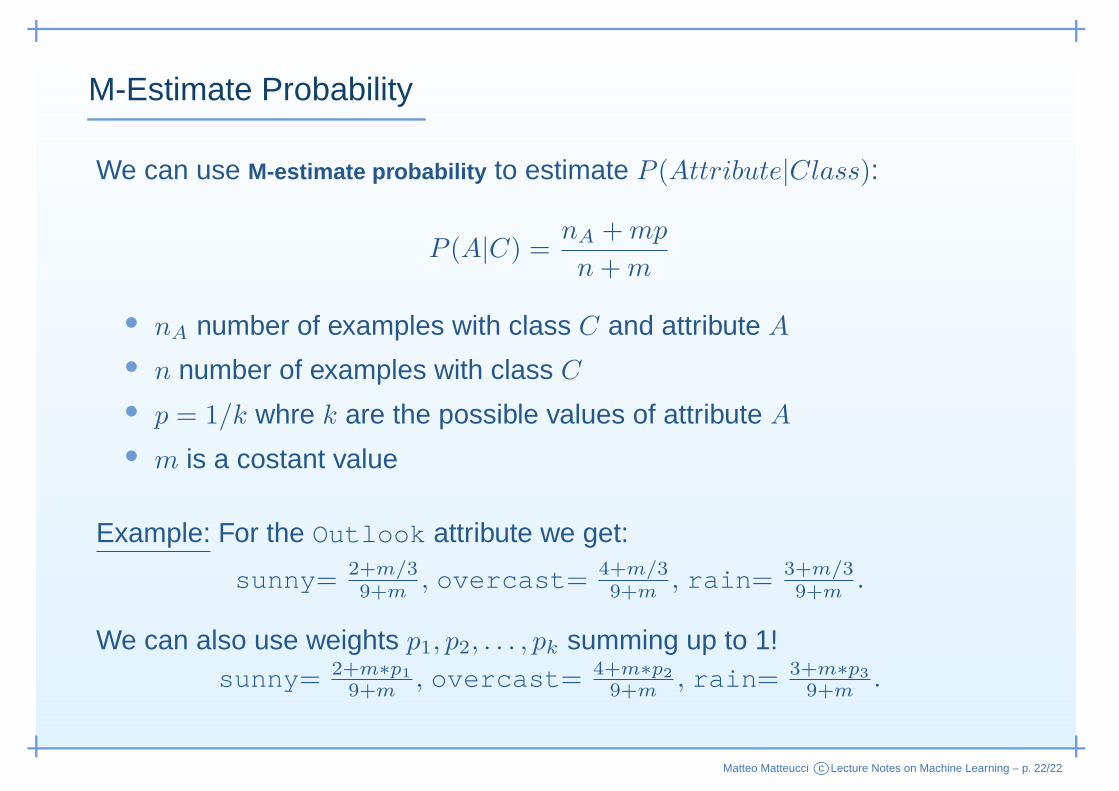
We can use M-estimate probability to estimate P (Attribute|Class):
P (A|C) =nA +mp
n+m
• nA number of examples with class C and attribute A
• n number of examples with class C
• p = 1/k whre k are the possible values of attribute A
• m is a costant value
Example: For the Outlook attribute we get:
sunny= 2+m/39+m , overcast= 4+m/3
9+m , rain= 3+m/39+m .
We can also use weights p1, p2, . . . , pk summing up to 1!sunny= 2+m∗p1
9+m , overcast= 4+m∗p2
9+m , rain= 3+m∗p3
9+m .
Matteo Matteucci c©Lecture Notes on Machine Learning – p. 22/22