Soft Labels for Ordinal Regression

Raul Dıaz, Amit Marathe

HP Inc.

{raul.diaz.garcia, amit.marathe}@hp.com

Abstract

Ordinal regression attempts to solve classification prob-

lems in which categories are not independent, but rather

follow a natural order. It is crucial to classify each class

correctly while learning adequate interclass ordinal rela-

tionships. We present a simple and effective method that

constrains these relationships among categories by seam-

lessly incorporating metric penalties into ground truth la-

bel representations. This encoding allows deep neural net-

works to automatically learn intraclass and interclass rela-

tionships without any explicit modification of the network

architecture. Our method converts data labels into soft

probability distributions that pair well with common cate-

gorical loss functions such as cross-entropy. We show that

this approach is effective by using off-the-shelf classifica-

tion and segmentation networks in four wildly different sce-

narios: image quality ranking, age estimation, horizon line

regression, and monocular depth estimation. We demon-

strate that our general-purpose method is very competitive

with respect to specialized approaches, and adapts well to

a variety of different network architectures and metrics.

1. Introduction

Ordinal classification, typically known as ordinal regres-

sion, is a type of machine learning task that resembles a

mixture of traditional regression of real-valued metrics, and

independent, multi-class classification problems. The goal

is to predict the category of an input instance from a discrete

set of labels, just like classification. Its main difference is

that the categories are related in a natural or implied order.

Common examples of such tasks are movie ratings (e.g., a

movie can be rated from 1 star to 5 stars) or customer sat-

isfaction surveys, where users are requested to respond to

certain questions from a range of answers with a logical or-

der (e.g., from ’poor’ to ’excellent’).

In a more broader view, ordinal regression attempts to

solve classification problems in which not all wrong classes

are equally wrong. Going back to the movie rating ex-

ample, if a particular movie has a true rating of 4 stars,

a mis-classification of 3 stars is less incorrect than a mis-

classification of 1 star. Obviously, the actual goal of the

system is to classify the movie as 4 stars. However, in the

event of not yielding the correct rating, it is desirable to out-

put a rating as close as possible to the ground truth one.

While classification in all its various forms (image and

object classification, segmentation, etc.) and metric re-

gression have always dominated most of the research chal-

lenges, ordinal regression is certainly not a novel problem

and has also been investigated for several years [21, 14, 9,

37]. Generally speaking, ordinal regression studies can be

classified either from those treating the problem as a version

of traditional metric regression in which the thresholds that

discretize the domain need to be estimated, or those who

frame the problem as a classification objective, by fixing a

set of thresholds on the domain space and learning classi-

fiers for each one of them.

When ordinal regression is approached from a regression

perspective, the literature tends to focus on mapping the in-

puts to a real line and predicting the boundaries between or-

dinal categories to define the final output class. Examples of

threshold approaches like [7, 6] use SVM or MAP respec-

tively to find the rank k of an input x given the boundaries band model weights w, either by finding the linear mapping

wTx ∈ [bk−1, bk] or by assuming that the latent function is

a Gaussian process.

Ordinal regression works from a classification point of

view typically assume a K-rank formulation by breaking the

problem domain into multiple ranks or thresholds. For in-

stance, [14] use K−1 binary classifiers, each one trained to

classify whether or not a particular input x has a response

y > k, where k is the rank for which the binary classifier is

trained. Alternatives using data replication methods can be

found in [29, 2]. Generally speaking, the ground truth rep-

resentation of ordinality is expressed by hard vectors: each

ground truth label generates K − 1 binary one-hot vectors

for each of the threshold classifiers. The rank prediction

of each input instance typically consists on the accumula-

tion of positive responses from the ensemble of these binary

classifiers. These type of approaches particularly suit well

on neural network architectures designed for classification.

14738

Our contribution. This paper presents a method that falls

into the category of ordinal regression approaches that view

the problem as a classification task. We present a soft tar-

get encoding scheme for data labels that provides a very

intuitive way of embedding ordinal information into ground

truth vectors. This encoding fits well in current state-of-the-

art, off-the-shelf deep convolutional neural networks (CNN)

that are originally designed for classification tasks. Unlike

other approaches, we show that these soft representations of

ordinal categories are able to outperform those using hard,

one-hot vectors.

2. Related Work

Ordinal regression has gained some momentum in the

past years, thanks to the increasing development and im-

provement of deep convolutional neural networks. Perhaps

the most popular approach is the K-rank method from [14],

but there are numerous alternatives to constrain interclass

and intraclass relationships for ordinal regression. We dis-

cuss previous works in the following paragraphs.

Soft methods. Alternatives to hard labels exist outside the

ordinal regression space. Soft loss terms have been useful

for domain and task transfer [41] in order to avoid dataset

biases. Elaborate loss functions are defined in [45] to take

into account the subjective scenicness of outdoor pictures,

by trying to predict the same rating distribution of human

annotations. Age estimation is a particular niche where soft

labels have become popular. In [39], age is represented by a

Gaussian distribution for which a lookup table is generated

beforehand to store multi-part integrals. These integrals ac-

count for the probability of an input image to belong to the

true chronological age of a given person, for whom multiple

age samples have been provided. Generally speaking, age

regression can be framed as an image ranking problem.

Image ranking. One popular use of ordinal regression in

Computer Vision is image ranking, where each image has to

be classified into a discrete set of equally spaced labels. Age

estimation is approached in [26] as an independent classifi-

cation problem by training a shallow convolutional network

to avoid overfitting. The same problem is addressed in [32]

by using a similar CNN with K − 1 binary classifiers, each

one designed to predict whether a particular image input

x contains a face older than a given age threshold y > k.

In order to enforce ordinality among age ranks, they add a

weight penalty wy,k in the categorical loss function equiv-

alent to the cost of predicting the input x of class y as rank

k. A different approach for image ranking is seen in [30],

who developed a deep neural network architecture that uses

multiple instances of the VGG-16 network [38] with shared

weights to constrain ordinal relationships. The network is

fed by tuples of inputs of different ranks or categories and

imposes a pairwise hinge loss alongside a Softmax logistic

regression loss. This approach shows excellent results in a

plethora of image ranking challenges with discrete ordinal

categories: age estimation, photographic quality, historical

dating of the picture, and image relevance.

Monocular depth estimation. Estimating pixel-wise

depth from RGB images is a particularly hot topic in Com-

puter Vision since it helps in numerous tasks related with

robotics and autonomous driving such as scene understand-

ing, 3D reconstruction, and 3D object analysis. Depth from

2D images is an essential task that has been extensively

approached by researchers [34, 1, 24, 35]. Since the in-

troduction of CNNs, results have improved dramatically

[49, 43, 11, 47, 12, 17]. Recently, ordinal regression was

introduced in monocular depth estimation challenges with

great results. The DORN network [15] outperformed state-

of-the-art results in challenging datasets like KITTI [16] or

Make3D [34]. DORN provides a novel depth discretization

strategy and a multi-scale network architecture. Their ap-

proach is based in the K-rank framework too, in which they

learn multiple binary classifiers to discern whether each

pixel in the image is closer or further away from each dis-

cretized depth threshold.

Horizon estimation. Many other challenges can be ap-

proached by ordinal regression. Generally speaking, any

task that involves a metric regression can be interpreted as

an ordinal regression task as long as the parameter space is

properly discretized. For example, horizon line estimation

has shown many benefits in scene understanding tasks from

monocular and multi-view points of view [22, 10]. Even

though solutions to find the horizon parameters are typi-

cally not formulated as ordinal regression problems, their

approaches certainly resemble them. In [48], a traditional

classification scheme is used to find discrete values of the

horizon line parameters and obtain candidates to estimate

the vanishing point of an image. In addition, [46] refine this

approach with a subwindow aggregation method. In [25],

the horizon is extracted as a potential semantic line by us-

ing two line pooling layers that are combined jointly with

both a classification and a regression layer.

3. Method

The most popular methods for ordinal regression use an

ensemble of multiple binary classifiers to determine the or-

dinal category for each input (K-rank approach). In this sec-

tion, we propose a simple and intuitive method that frames

ordinal regression as a traditional classification problem. In

other words, we expect our deep neural network’s last layer

to have as many output neurons as categories or ranks we

intend to classify, instead of twice as many. We do not per-

form any explicit modification in any network architecture.

Our contribution relies on exclusively in how we present the

ground truth information to the network.

4739

3.1. Encoding Regression as Classification

Classification is typically carried out by describing each

category in a one-hot coded vector, where all values are

zeroed out except the one indicating the true class, whose

value is 1. Training is performed with a categorical loss

function such as cross-entropy. The activation of the output

layer of the neural network in a classification scenario is

typically Softmax, so both the network output and the true

labels (one-hot vectors) are probability distributions that we

intend to match via the loss function. Intuitively, the net-

work will learn how to mimic these one-hot coded vectors

as much as possible, so that the argmax value of its output

layer corresponds to the true class of the input.

In an independent class scenario, the order in which

these classes are set up does not matter. This is expressed

in the one-hot coded vectors, where we zero out the chance

of any wrong class to be remotely similar to the true class.

In other words, we set all wrong classes to be infinitely far

away from the true class. However, this is not the case for

ordinal regression, where there exist certain categories that

are more correct than others with respect to the true label.

The K-rank approaches solve this problem by hardcod-

ing each class into multiple binary 1-hot vectors and by

aggregating the response of each binary classifier. This

method forces each data label to be necessarily assigned in

a hard way to one of the ordinal categories or ranks, thus

losing valuable information in cases were labels belong to a

continuous domain. Each classifier is then trained to learn

exclusively a binary response for each specified rank thresh-

old, often isolating its optimization with respect to the other

threshold classifiers in the ensemble.

We propose that the ordinality of the different ranks can

be expressed easily without the necessity of these multiple

binary classifiers. In the end, a classification network will

always try to estimate the likelihood of an input to belong to

a certain class. For naturally ordered classes, we know that

this likelihood can be expressed by their interclass distance.

Hence, we introduce a novel formulation to describe cat-

egories that naturally encapsulates explicit order relations

among classes. In particular, let Y = {r1, r2, ..., rK} be the

K ordinal categories (or ranks) of our classification prob-

lem. We compute an encoded vector as our ground truth

label y for a particular instance of rank rt as:

yi =e−φ(rt,ri)

∑Kk=1 e

−φ(rt,rk)∀ri ∈ Y (1)

where φ(rt, ri) is a metric loss function of our choice

that penalizes how far the true metric value of rt is from the

rank ri ∈ Y . This formulation, which we name Soft Ordi-

nal vectors (or SORD), resembles that of a Softmax layer

where metric penalties are encoded in a softly normalized

probability distribution. In this form, the element that is the

closest (or matches) the true ordinal class will have the high-

est value like in a classification problem (but not necessarily

1). Nearby categories will have smaller and smaller values

as they move far from the true class (but not necessarily 0).

Hence, these soft labels naturally encapsulate the rank like-

lihoods of an input instance given a pre-defined interclass

penalty distance φ.

Like in a standard regression problem, the choice of this

penalty function depends on the problem that needs to be

solved and the desired performance of the approach. We

can use any metric loss as the penalty function φ, such as the

absolute or squared error, but many other metrics can be nat-

urally adapted in these soft vectors. Encoding ground truth

labels as probability distributions also pairs well with com-

mon classification loss functions that use a Softmax output

such as cross-entropy or the Kullback-Leibler divergence,

because these loss functions target the minimization of the

area between a network’s Softmax output and the ground

truth vector representations.

3.2. Backpropagation of Metrics

A great advantage of encoding ordinal information in

this form is the fact that the gradient of the categorical loss

function also becomes fairly easy to compute. Let us as-

sume the use of a loss function such as cross-entropy, with

a gradient of ∂L∂pi

= − yi

pi

. Here, yi is the element of a soft

label vector for rank ri as in equation 1, and pi is the net-

work’s Softmax value of the logit output node oi that cor-

responds to the same rank. Given an input of true rank rt,let C > 0 be a constant such that the Softmax denominator

matches the SORD denominator:

C

K∑

k=1

eok =

K∑

k=1

eok+logC =

K∑

k=1

e−φ(rt,rk) (2)

Let o′i = oi + logC be this set of biased logits. This

offset-invariance property of Softmax allows the cancella-

tion of both denominators, simplifying the gradient of the

loss function with respect to the network output to:

∂L

∂pi= −

e−φ(rt,ri)

eo′

i

= −e−φ(rt,ri)−o′i (3)

Backpropagation in all other layers is performed by stan-

dard procedure. Intuitively, SORD trains the network to

yield higher values in the nodes which are closer to the true

class, and smaller values in classes that are further away.

The classification loss (e.g., cross-entropy) will penalize

each output logit value oi if it does not respect the inter-

class distance φ with respect to the true rank rt and offset

logC, making the loss reach its minima when:

oi + logC = −φ(rt, ri) ∀ri ∈ Y (4)

4740

3.3. SORD Properties

Our soft ordinal labels have many advantages over other

existing methods. First, their formulation is very easy to

reproduce. Its simplest expression can be written in just

two lines of code: 1) compute φ(rt, ri) for all ri ∈ Y;

2) generate the soft label y by simply computing Softmax

of all −φ(rt, ri). Second, we can use well known classi-

fication architectures for the purpose of ordinal regression

without explicitly modifying a single layer: unlike K-rank

approaches that need twice as many parameters to define

all binary rank classifiers in the last layer, we maintain the

same number of output neurons as ranks are defined in the

problem. Third, we can either use the argmax of the out-

put layer as our prediction at inference time, or use a simple

expected value formula like∑K

k=1 rkpk.

Finally, SORD is able to easily encapsulate data from a

continuous domain. For instance, let an input instance have

a true depth value rt = 2.3m /∈ Y in a monocular depth

estimation problem. Rather than hard-assigning this input

to the closest rank, we compute φ normally. If there exist

two consecutive ranks ri = 2m and ri+1 = 3m, a SORD

vector y will smoothly balance itself towards ri, but not as

strongly as an input with a label r′t = 2.1m and SORD vec-

tor y′. Hence, every possible real value in the domain will

generate a slightly different soft label that will lean towards

each ordinal category stronger or weaker according to their

continuous distance metric likelihood.

4. Experimental Results

In order to evaluate the benefits of our ordinal regression

approach, we present a number of experiments that cover

wildly different task scenarios, classification architectures,

and ordinal label distributions. We benchmark our SORD

labels in four different datasets. First, use the Image Aes-

thetics dataset [36] and the Adience dataset [26] to eval-

uate our method on uniformly distributed class scenarios

for image quality and age estimation respectively. Second,

we test our approach against the recently renewed, well-

known KITTI dataset [42]. Here, we use SORD to predict

depth from RGB images, following the incremental SID

discretization of [15]. Finally, we test a multivariate regres-

sion scenario, where we estimate the horizon line parame-

ters of the Horizon Lines in the Wild dataset [46].

Setup. Our setup consists of a computer with an Intel i7

processor and an NVIDIA GTX 1080Ti GPU. We imple-

ment our experiments by using the high level deep learning

platform Keras [5]. We use pre-trained networks, for which

the last layer is set up with random weights and a learning

rate 10 times larger than the one given for all other lay-

ers, following [30]. We reduce the learning rate by a factor

of ×0.1 when the error plateaus. Our optimization choice

is Stochastic Gradient Descent (SGD) with a momentum

of 0.9. Without loss of generality, we adopt the Kullback-

Leibler divergence as our classification loss: by subtracting

the SORD vector entropy, our loss value would lead to 0.0in case there was a perfect match between the network out-

put and our soft ordinal labels.

4.1. Image Ranking

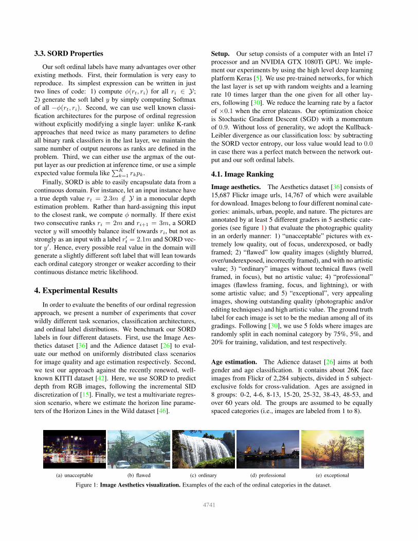
Image aesthetics. The Aesthetics dataset [36] consists of

15,687 Flickr image urls, 14,767 of which were available

for download. Images belong to four different nominal cate-

gories: animals, urban, people, and nature. The pictures are

annotated by at least 5 different graders in 5 aesthetic cate-

gories (see figure 1) that evaluate the photographic quality

in an orderly manner: 1) “unacceptable” pictures with ex-

tremely low quality, out of focus, underexposed, or badly

framed; 2) “flawed” low quality images (slightly blurred,

over/underexposed, incorrectly framed), and with no artistic

value; 3) “ordinary” images without technical flaws (well

framed, in focus), but no artistic value; 4) “professional”

images (flawless framing, focus, and lightning), or with

some artistic value; and 5) “exceptional”, very appealing

images, showing outstanding quality (photographic and/or

editing techniques) and high artistic value. The ground truth

label for each image is set to be the median among all of its

gradings. Following [30], we use 5 folds where images are

randomly split in each nominal category by 75%, 5%, and

20% for training, validation, and test respectively.

Age estimation. The Adience dataset [26] aims at both

gender and age classification. It contains about 26K face

images from Flickr of 2,284 subjects, divided in 5 subject-

exclusive folds for cross-validation. Ages are assigned in

8 groups: 0-2, 4-6, 8-13, 15-20, 25-32, 38-43, 48-53, and

over 60 years old. The groups are assumed to be equally

spaced categories (i.e., images are labeled from 1 to 8).

(a) unacceptable (b) flawed (c) ordinary (d) professional (e) exceptional

Figure 1: Image Aesthetics visualization. Examples of the each of the ordinal categories in the dataset.

4741

Accuracy (%) - higher is better MAE - lower is better

RED- CNNm Niu et CNN-SORD

RED- CNNm Niu et CNN-SORD

SVM [29] [30] al [32] POR [30] SVM [29] [30] al [32] POR [30]

Nature 70.72 70.97 69.81 71.86 73.59 0.309 0.305 0.313 0.294 0.271

Animal 61.05 68.02 69.10 69.32 70.29 0.410 0.342 0.331 0.322 0.308

Urban 65.44 68.19 66.49 69.09 73.25 0.356 0.374 0.349 0.325 0.276

People 61.16 71.63 70.44 69.94 70.59 0.315 0.412 0.312 0.321 0.309

Overall 64.59 69.45 68.96 70.05 72.03 0.330 0.376 0.326 0.316 0.290

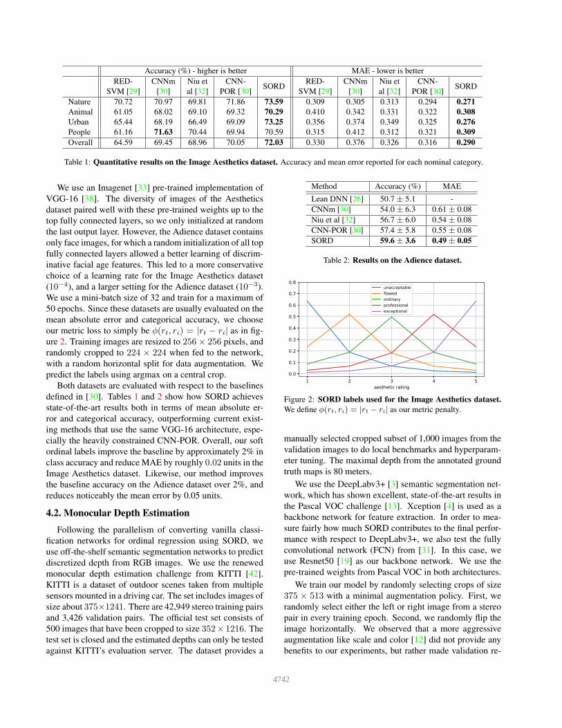
Table 1: Quantitative results on the Image Aesthetics dataset. Accuracy and mean error reported for each nominal category.

We use an Imagenet [33] pre-trained implementation of

VGG-16 [38]. The diversity of images of the Aesthetics

dataset paired well with these pre-trained weights up to the

top fully connected layers, so we only initialized at random

the last output layer. However, the Adience dataset contains

only face images, for which a random initialization of all top

fully connected layers allowed a better learning of discrim-

inative facial age features. This led to a more conservative

choice of a learning rate for the Image Aesthetics dataset

(10−4), and a larger setting for the Adience dataset (10−3).

We use a mini-batch size of 32 and train for a maximum of

50 epochs. Since these datasets are usually evaluated on the

mean absolute error and categorical accuracy, we choose

our metric loss to simply be φ(rt, ri) = |rt − ri| as in fig-

ure 2. Training images are resized to 256× 256 pixels, and

randomly cropped to 224 × 224 when fed to the network,

with a random horizontal split for data augmentation. We

predict the labels using argmax on a central crop.

Both datasets are evaluated with respect to the baselines

defined in [30]. Tables 1 and 2 show how SORD achieves

state-of-the-art results both in terms of mean absolute er-

ror and categorical accuracy, outperforming current exist-

ing methods that use the same VGG-16 architecture, espe-

cially the heavily constrained CNN-POR. Overall, our soft

ordinal labels improve the baseline by approximately 2% in

class accuracy and reduce MAE by roughly 0.02 units in the

Image Aesthetics dataset. Likewise, our method improves

the baseline accuracy on the Adience dataset over 2%, and

reduces noticeably the mean error by 0.05 units.

4.2. Monocular Depth Estimation

Following the parallelism of converting vanilla classi-

fication networks for ordinal regression using SORD, we

use off-the-shelf semantic segmentation networks to predict

discretized depth from RGB images. We use the renewed

monocular depth estimation challenge from KITTI [42].

KITTI is a dataset of outdoor scenes taken from multiple

sensors mounted in a driving car. The set includes images of

size about 375×1241. There are 42,949 stereo training pairs

and 3,426 validation pairs. The official test set consists of

500 images that have been cropped to size 352× 1216. The

test set is closed and the estimated depths can only be tested

against KITTI’s evaluation server. The dataset provides a

Method Accuracy (%) MAE

Lean DNN [26] 50.7 ± 5.1 -

CNNm [30] 54.0 ± 6.3 0.61 ± 0.08

Niu et al [32] 56.7 ± 6.0 0.54 ± 0.08

CNN-POR [30] 57.4 ± 5.8 0.55 ± 0.08

SORD 59.6 ± 3.6 0.49 ± 0.05

Table 2: Results on the Adience dataset.

1 2 3 4 5aesthetic rating

0.0

0.1

0.2

0.3

0.4

0.5

0.6

0.7

0.8unacceptableflawedordinaryprofessionalexceptional

Figure 2: SORD labels used for the Image Aesthetics dataset.

We define φ(rt, ri) = |rt − ri| as our metric penalty.

manually selected cropped subset of 1,000 images from the

validation images to do local benchmarks and hyperparam-

eter tuning. The maximal depth from the annotated ground

truth maps is 80 meters.

We use the DeepLabv3+ [3] semantic segmentation net-

work, which has shown excellent, state-of-the-art results in

the Pascal VOC challenge [13]. Xception [4] is used as a

backbone network for feature extraction. In order to mea-

sure fairly how much SORD contributes to the final perfor-

mance with respect to DeepLabv3+, we also test the fully

convolutional network (FCN) from [31]. In this case, we

use Resnet50 [19] as our backbone network. We use the

pre-trained weights from Pascal VOC in both architectures.

We train our model by randomly selecting crops of size

375 × 513 with a minimal augmentation policy. First, we

randomly select either the left or right image from a stereo

pair in every training epoch. Second, we randomly flip the

image horizontally. We observed that a more aggressive

augmentation like scale and color [12] did not provide any

benefits to our experiments, but rather made validation re-

4742

higher is better lower is better

Network φ δ < 1.25 δ < 1.252 δ < 1.253 absErrorRel sqErrorRel RMSE RMSElog SILog

FCN

SQ 92.75 98.52 99.46 8.38 2.25 3.45 0.132 12.50

SI 92.19 98.65 99.62 9.12 2.04 3.41 0.131 12.00

SL 93.14 98.78 99.62 7.98 1.73 3.31 0.124 11.73

DeepLabv3+

SQUD 95.35 98.96 99.59 7.29 1.43 3.10 0.114 10.68

SQ 95.54 99.04 99.63 6.93 1.42 2.98 0.110 10.32

SI 95.08 99.11 99.71 7.09 1.31 2.95 0.109 10.20

SL 95.10 99.17 99.74 7.07 1.31 2.92 0.107 9.99

SQCS+EV 95.41 99.01 99.69 7.07 1.59 2.85 0.108 10.12

SLCS 95.77 99.21 99.75 6.99 1.27 2.86 0.104 9.73

Table 3: Quantitative results for the KITTI dataset. Values obtained from the official validation subset using the SID discretization,

argmax prediction, and pre-trained weights from Pascal VOC, except for: uniform discretization (UD), pre-trained weights from Cityscapes

(CS), and expected value prediction (EV). The squared log difference (SL) and SILog (SI) obtain better results than the squared difference

(SQ). Overall, the former performs slightly better. Delta thresholds, relative errors, and SILog metrics are multiplied by 100 for readability.

sults worse. We apply a Nesterov momentum of 0.9, along-

side a mini-batch size of 4 images. We train for 30 epochs,

which corresponds approximately to 300k iterations. We

only compute the loss in those image pixels with an asso-

ciated ground truth value. At test time, we zero-pad the

cropped images to recover the original height and width

from the training set. Following [15], we adopt their SID

strategy, extract equally spaced crops alongside the hori-

zontal axis, and average the areas where two or more crops

overlap to infer the depth values.

We explore different interclass distances as our φ metric

losses. We first use two pixel-wise depth measures. Given a

pixel p with ground truth depth rt and a discrete depth rank

value ri from SID, we define the square difference and the

square log difference as:

φ(rt, ri) = ‖rt − ri‖2 (5)

φ(rt, ri) = ‖ log rt − log ri‖2 (6)

Inspired by [12], we also build a pixel-wise version for

the Scale-Invariant logarithmic error as:

φ(rt, ri) = d2rt,ri −drt,rin

(drt,ri +∑

p′ 6=p

dp′) (7)

where drt,ri = log ri − log rt, and dp′ = log r′i − log r′tcomputes the log difference of the ground truth value r′t and

the current depth prediction r′i for any other pixel p′ in the

image. Intuitively, equation 7 computes how much a change

only in the prediction of pixel p contributes to the image-

wise SILog error, assuming that predictions for all other

pixels would remain the same. Hence, this metric penalizes

pixel-wise depth predictions in the opposite direction of the

current average depth error, and credits those that have a

similar one.

1.0 1.5 2.4 3.7 5.8 8.9 13.9 21.5 33.3 51.6 80.0depth (m)

0.0

0.2

0.4

0.6

0.8 3 meters10 meters50 meters

1.0 1.5 2.4 3.7 5.8 8.9 13.9 21.5 33.3 51.6 80.0depth (m)

0.00

0.01

0.023 meters10 meters50 meters

Figure 3: SORD labels under SID discretization. We use K =120 intervals. Top: equation 5. Bottom: equation 6.

We benchmark and finetune our approach by using the

official validation subset of 1,000 cropped images before

submitting our results to the KITTI test server. We use the

same evaluation metrics as in [12]. Table 3 shows our multi-

ple experiments. We observe how the squared log difference

obtains better overall results compared to the other metrics,

improving the pixel-wise SILog metric and the squared dif-

ference. As expected, SID performs better than a uniformly

discretized depth space. FCN achieves good results with a

SILog of 11.73, while DeepLabv3+ reduces this error up

to 9.99. A final set of experiments is conducted by using

the pre-trained weights of the Cityscapes dataset [8], which

are specific to the domain of autonomous driving. This al-

lows the reduction of the SILog error up to 9.73 with re-

spect to equation 6. Table 4 shows that this latter setup is

competitive and achieves the second best rating among the

published methods in the official test set, only outperformed

by DORN. Figure 3 shows examples of the SORD vectors

used. Estimated depths are shown in figure 4.

4743

Image Ground Truth DeepLabv3+ (SQ) DeepLabv3+ (SL) FCN (SI)

Figure 4: Qualitative results on the KITTI dataset. Examples of how the different metrics generate depth maps. Compared to the

squared log metric (SL), the squared difference (SQ) is able to retrieve finer details (trees, railings, etc.), but yields slightly worse results.

As expected, DeepLabv3+ predicts depth better compared to FCN. Ground truth has been interpolated for visualization.

Method SILog sqErrorRel absErrorRel iRMSE

DORN [15] 11.77 2.23 8.78 12.98

SORD 12.39 2.49 10.10 13.48

VGG16-UNet [18] 13.41 2.86 10.60 15.06

DABC [27] 14.49 4.08 12.72 15.53

APMoE [23] 14.74 3.88 11.74 15.63

Table 4: Quantitative results on the KITTI benchmark server.

SORD achieves the second place in the official online rankings,

outperforming specialized depth estimation methods.

Number of intervals. Discretizing the output domain

contributes to predicting depth values more precisely. There

is not a magic number of intervals to set, and this number

typically depends on the task to solve and its domain. As

stated in [15], having too few intervals leads to quantiza-

tion errors, while having too many intervals tends to lose

the benefits of discretization. We explored the sensitivity

of SORD to the number of intervals, by evaluating SID in

a wide range of them (80 to 160). For this ablation study,

we used φ as in equation 5. Figure 5 shows how our soft

labels reach their best performance around K = 120 SID

intervals. It is important to note that SORD tends to plateau

beyond the optimal number of intervals, and that its perfor-

mance does not decay as fast as it does when we use fewer

intervals than the optimal number. This indicates that our

soft ordinal labels also adapt well to the sensitivity of SID,

even at a higher number of intervals than DORN [15].

80 100 120 140 160intervals

94.50

94.75

95.00

95.25

delta

< 1

.25

80 100 120 140 160intervals

3.05

3.10

3.15

RMSE

80 100 120 140 160intervals

1.5

1.6

1.7

Squa

Rel

80 100 120 140 160intervals

10.6

10.8

11.0

SILo

g

Figure 5: SORD performance on different SID intervals. We

observed that our soft ordinal labels are robust to a wide variety of

intervals, and acquired the best results at K = 120.

SORD entropy. We observed that the entropy of our soft

labels had influence over other hyperparameters. For in-

stance, φ performed better when using a learning rate of

10−3 in equation 5 and 10−1 when using equations 6 and

7. The larger the entropy of SORD, the smaller the mag-

nitude of the gradients when performing backpropagation,

hence the need of a bigger learning rate to avoid falling in

a local minima in the early stages of training. At inference

time, we observed that argmax performed better than the ex-

pected value prediction when SORD accounts for the con-

4744

tribution of each rank more evenly: our DeepLabv3+ tests

with equation 6 obtained very poor results when computing

the expected value, with a SILog of 15.06. However, table

3 shows how the expected value does improve results when

using the smaller entropy vectors of equation 5.

4.3. Horizon Estimation

Figuring out the horizon line is an important feature for

scene understanding tasks, in which two parameters need

to be estimated: the angle θ ∈ [−π2 ,

π2 ] with respect to the

horizontal axis, and the signed offset ρ ∈ [− inf, inf], which

defines the closest distance of the horizon line and the im-

age center. This illustrates a great example of how SORD

performs in a multivariate ordinal regression case: by bring-

ing two parameters of very different domains into the same

discrete probability distribution space, this time we aim to

minimize the volume between the surfaces of the joint dis-

tributions of two network outputs and two SORD vectors.

We use the Horizon Lines in the Wild dataset [46] for

this purpose. HLW consists of a curated selection of images

from high quality Structure from Motion models from the

1DSfM, Landmarks, and YFCC100M datasets [44, 28, 20].

The horizon parameters are extracted from the SfM data and

projected into each image plane. HLW contains about 100K

images divided in 96,617, 525, and 2,018 images for train-

ing, validation, and test respectively.

We use the Resnet50 [19] network pre-trained from Im-

agenet. We substitute the last fully connected output layer

by two disjoint fully connected layers, each one dedicated

to predict each of the two parameters θ (in degrees) and ρ (in

pixels). The ranks are determined by a linear interpolation

of N = 100 bins from the cumulative distribution of each

parameter in the training data, following [46]. At training

time, we resize each image to have 256 pixels in the shorter

dimension, and randomly extract 224 × 224 crops that are

randomly flipped horizontally. We use a learning rate of

10−3, and a mini-batch size of 32. We train for a maximum

of 50 epochs. At inference time, we resize the test images

to have 224 pixels in their shorter dimension, and extract a

central crop to estimate the horizon line parameters with re-

spect to the original image size. We use as interclass metrics

the squared difference error of each parameter:

φθ(θt, θi) = min(‖θt − θi‖2,

‖(θt − θi − π) mod 2π‖2)(8)

φρ(ρt, ρi) = ‖ρt − ρi‖2 (9)

We compare our multivariate SORD approach with the

HLW baseline method of [46], and the more recent semantic

line extraction method from [25]. We test both the argmax

and the expected value as predictions at inference time. Ta-

ble 5 benchmarks the results using the area under the curve

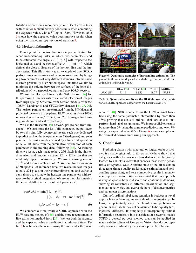
Figure 6: Qualitative examples of horizon line estimation. The

ground truth lines are depicted in a dashed green line, while our

estimation is drawn in yellow.

HLW [46] SLNet [25] SORD SORDEV

AUC (%) 71.16 82.33 88.77 89.98

Table 5: Quantitative results on the HLW dataset. Our multi-

variate SORD approach outperforms the baseline over 7%.

score of [40]. SORD outperforms the HLW original base-

line using the same parameter interpolation by more than

18%, proving that our soft ordinal labels are able to out-

perform hard label assignments. We improve SLNet results

by more than 6% using the argmax prediction, and over 7%

using the expected value (EV). Figure 6 shows examples of

the estimated horizon lines using our approach.

5. Conclusion

Predicting classes with a natural or logical order associ-

ated is a challenging task. In this paper, we have shown that

categories with a known interclass distance can be jointly

learned by a K-class vector that encodes these metric penal-

ties a la Softmax. SORD obtains state-of-the-art results in

three tasks (image quality ranking, age estimation, and hori-

zon line regression), and very competitive results in monoc-

ular depth estimation. We demonstrated that our approach

is very adaptative both in discrete and continuous domains,

showing its robustness in different classification and seg-

mentation networks, and over a plethora of distance metrics

and parameter discretizations.

Our soft ordinal label representation introduces a novel

approach not only to regression and ordinal regression prob-

lems, but potentially even for classification problems in

general where labels may not be assumed to be equally (i.e.,

infinitely) different. Its simplicity at incorporating ordinal

information seamlessly into classification networks makes

SORD a general-purpose method that can be applied in

many subdisciplines of Computer Vision that do not typi-

cally consider ordinal regression as a possible solution.

4745

References

[1] Mohammad Haris Baig and Lorenzo Torresani. Coupled

depth learning. In IEEE Winter Conference on Applications

of Computer Vision (WACV), pages 1–10. IEEE, 2016. 2

[2] Jaime S Cardoso and Joaquim F Costa. Learning to clas-

sify ordinal data: The data replication method. Journal of

Machine Learning Research, 8(Jul):1393–1429, 2007. 1

[3] Liang-Chieh Chen, Yukun Zhu, George Papandreou, Florian

Schroff, and Hartwig Adam. Encoder-decoder with atrous

separable convolution for semantic image segmentation. In

Proceedings of the European Conference on Computer Vi-

sion (ECCV), pages 801–818, 2018. 5

[4] Francois Chollet. Xception: Deep learning with depthwise

separable convolutions. In Proceedings of the IEEE Con-

ference on Computer Vision and Pattern Recognition, pages

1251–1258, 2017. 5

[5] Francois Chollet et al. Keras. https://keras.io, 2015.

4

[6] Wei Chu and Zoubin Ghahramani. Gaussian processes for

ordinal regression. Journal of machine learning research,

6(Jul):1019–1041, 2005. 1

[7] Wei Chu and S Sathiya Keerthi. Support vector ordinal re-

gression. Neural computation, 19(3):792–815, 2007. 1

[8] Marius Cordts, Mohamed Omran, Sebastian Ramos, Timo

Rehfeld, Markus Enzweiler, Rodrigo Benenson, Uwe

Franke, Stefan Roth, and Bernt Schiele. The cityscapes

dataset for semantic urban scene understanding. In The

IEEE Conference on Computer Vision and Pattern Recog-

nition (CVPR), June 2016. 6

[9] Koby Crammer and Yoram Singer. Pranking with ranking.

In Advances in neural information processing systems, pages

641–647, 2002. 1

[10] Raul Dıaz, Sam Hallman, and Charless C Fowlkes. Detecting

dynamic objects with multi-view background subtraction. In

Proceedings of the IEEE International Conference on Com-

puter Vision, pages 273–280, 2013. 2

[11] David Eigen and Rob Fergus. Predicting depth, surface nor-

mals and semantic labels with a common multi-scale con-

volutional architecture. In Proceedings of the IEEE Inter-

national Conference on Computer Vision, pages 2650–2658,

2015. 2

[12] David Eigen, Christian Puhrsch, and Rob Fergus. Depth map

prediction from a single image using a multi-scale deep net-

work. In Advances in neural information processing systems,

pages 2366–2374, 2014. 2, 5, 6

[13] Mark Everingham, Luc Van Gool, Christopher KI Williams,

John Winn, and Andrew Zisserman. The pascal visual object

classes (VOC) challenge. International journal of computer

vision, 88(2):303–338, 2010. 5

[14] Eibe Frank and Mark Hall. A simple approach to ordinal

classification. In European Conference on Machine Learn-

ing, pages 145–156, 2001. 1, 2

[15] Huan Fu, Mingming Gong, Chaohui Wang, Kayhan Bat-

manghelich, and Dacheng Tao. Deep ordinal regression net-

work for monocular depth estimation. In Proceedings of the

IEEE Conference on Computer Vision and Pattern Recogni-

tion, pages 2002–2011, 2018. 2, 4, 6, 7

[16] Andreas Geiger, Philip Lenz, Christoph Stiller, and Raquel

Urtasun. Vision meets robotics: The KITTI dataset. The

International Journal of Robotics Research, 32(11):1231–

1237, 2013. 2

[17] Clement Godard, Oisin Mac Aodha, and Gabriel J Bros-

tow. Unsupervised monocular depth estimation with left-

right consistency. In Proceedings of the IEEE Conference on

Computer Vision and Pattern Recognition, pages 270–279,

2017. 2

[18] Xiaoyang Guo, Hongsheng Li, Shuai Yi, Jimmy Ren, and

Xiaogang Wang. Learning monocular depth by distilling

cross-domain stereo networks. In Proceedings of the Euro-

pean Conference on Computer Vision (ECCV), pages 484–

500, 2018. 7

[19] Kaiming He, Xiangyu Zhang, Shaoqing Ren, and Jian Sun.

Deep residual learning for image recognition. In Proceed-

ings of the IEEE Conference on Computer Vision and Pattern

Recognition, pages 770–778, 2016. 5, 8

[20] Jared Heinly, Johannes L Schonberger, Enrique Dunn, and

Jan-Michael Frahm. Reconstructing the world* in six

days*(as captured by the yahoo 100 million image dataset).

In Proceedings of the IEEE Conference on Computer Vision

and Pattern Recognition, pages 3287–3295, 2015. 8

[21] Ralf Herbrich, Thore Graepel, and Klaus Obermayer. Sup-

port vector learning for ordinal regression. International

Conference on Artificial Neural Networks (ICANN), 1999.

1

[22] Derek Hoiem, Alexei A Efros, and Martial Hebert. Putting

objects in perspective. International Journal of Computer

Vision, 80(1):3–15, 2008. 2

[23] Shu Kong and Charless Fowlkes. Pixel-wise attentional gat-

ing for scene parsing. In 2019 IEEE Winter Conference on

Applications of Computer Vision (WACV), pages 1024–1033.

IEEE, 2019. 7

[24] Lubor Ladicky, Jianbo Shi, and Marc Pollefeys. Pulling

things out of perspective. In Proceedings of the IEEE Con-

ference on Computer Vision and Pattern Recognition, pages

89–96, 2014. 2

[25] Jun-Tae Lee, Han-Ul Kim, Chul Lee, and Chang-Su Kim.

Semantic line detection and its applications. In The IEEE

International Conference on Computer Vision (ICCV), Oct

2017. 2, 8

[26] Gil Levi and Tal Hassner. Age and gender classification us-

ing convolutional neural networks. In Proceedings of the

IEEE Conference on Computer Vision and Pattern Recogni-

tion Workshops, pages 34–42, 2015. 2, 4, 5

[27] Ruibo Li, Ke Xian, Chunhua Shen, Zhiguo Cao, Hao Lu, and

Lingxiao Hang. Deep attention-based classification network

for robust depth prediction. In Proceedings of the Asian Con-

ference on Computer Vision (ACCV), 2018. 7

[28] Yunpeng Li, Noah Snavely, Dan Huttenlocher, and Pascal

Fua. Worldwide pose estimation using 3D point clouds.

In European Conference on Computer Vision, pages 15–29.

Springer, 2012. 8

[29] Hsuan-Tien Lin and Ling Li. Reduction from cost-sensitive

ordinal ranking to weighted binary classification. Neural

Computation, 24(5):1329–1367, 2012. 1, 5

4746

[30] Yanzhu Liu, Adams Wai Kin Kong, and Chi Keong Goh.

A constrained deep neural network for ordinal regression.

In Proceedings of the IEEE Conference on Computer Vision

and Pattern Recognition, pages 831–839, 2018. 2, 4, 5

[31] Jonathan Long, Evan Shelhamer, and Trevor Darrell. Fully

convolutional networks for semantic segmentation. In Pro-

ceedings of the IEEE Conference on Computer Vision and

Pattern Recognition, pages 3431–3440, 2015. 5

[32] Zhenxing Niu, Mo Zhou, Le Wang, Xinbo Gao, and Gang

Hua. Ordinal regression with multiple output CNN for age

estimation. In Proceedings of the IEEE Conference on Com-

puter Vision and Pattern Recognition, pages 4920–4928,

2016. 2, 5

[33] Olga Russakovsky, Jia Deng, Hao Su, Jonathan Krause, San-

jeev Satheesh, Sean Ma, Zhiheng Huang, Andrej Karpathy,

Aditya Khosla, Michael Bernstein, Alexander C. Berg, and

Li Fei-Fei. ImageNet Large Scale Visual Recognition Chal-

lenge. International Journal of Computer Vision (IJCV),

115(3):211–252, 2015. 5

[34] Ashutosh Saxena, Sung H Chung, and Andrew Y Ng. Learn-

ing depth from single monocular images. In Advances in

neural information processing systems, pages 1161–1168,

2006. 2

[35] Ashutosh Saxena, Min Sun, and Andrew Y Ng. Make3D:

Learning 3D scene structure from a single still image. IEEE

Transactions on Pattern Analysis and Machine Intelligence,

31(5):824–840, 2009. 2

[36] Rossano Schifanella, Miriam Redi, and Luca Maria Aiello.

An image is worth more than a thousand favorites: Surfacing

the hidden beauty of flickr pictures. In Ninth International

AAAI Conference on Web and Social Media, 2015. 4

[37] Amnon Shashua and Anat Levin. Ranking with large margin

principle: Two approaches. In Advances in neural informa-

tion processing systems, pages 961–968, 2003. 1

[38] Karen Simonyan and Andrew Zisserman. Very deep convo-

lutional networks for large-scale image recognition. arXiv

preprint arXiv:1409.1556, 2014. 2, 5

[39] Zichang Tan, Shuai Zhou, Jun Wan, Zhen Lei, and Stan Z Li.

Age estimation based on a single network with soft softmax

of aging modeling. In Asian Conference on Computer Vision,

pages 203–216. Springer, 2016. 2

[40] Elena Tretyak, Olga Barinova, Pushmeet Kohli, and Vic-

tor Lempitsky. Geometric image parsing in man-made

environments. International Journal of Computer Vision,

97(3):305–321, 2012. 8

[41] Eric Tzeng, Judy Hoffman, Trevor Darrell, and Kate Saenko.

Simultaneous deep transfer across domains and tasks. In

Proceedings of the IEEE International Conference on Com-

puter Vision, pages 4068–4076, 2015. 2

[42] Jonas Uhrig, Nick Schneider, Lukas Schneider, Uwe Franke,

Thomas Brox, and Andreas Geiger. Sparsity invariant CNNs.

In International Conference on 3D Vision (3DV), pages 11–

20. IEEE, 2017. 4, 5

[43] Xiaolong Wang, David Fouhey, and Abhinav Gupta. Design-

ing deep networks for surface normal estimation. In Pro-

ceedings of the IEEE Conference on Computer Vision and

Pattern Recognition, pages 539–547, 2015. 2

[44] Kyle Wilson and Noah Snavely. Robust global translations

with 1dsfm. In European Conference on Computer Vision,

pages 61–75, 2014. 8

[45] Scott Workman, Richard Souvenir, and Nathan Jacobs. Un-

derstanding and mapping natural beauty. In Proceedings

of the IEEE International Conference on Computer Vision,

pages 5589–5598, 2017. 2

[46] Scott Workman, Menghua Zhai, and Nathan Jacobs. Horizon

lines in the wild. In BMVC, 2016. 2, 4, 8

[47] Junyuan Xie, Ross Girshick, and Ali Farhadi. Deep3D: Fully

automatic 2D-to-3D video conversion with deep convolu-

tional neural networks. In European Conference on Com-

puter Vision, pages 842–857. Springer, 2016. 2

[48] Menghua Zhai, Scott Workman, and Nathan Jacobs. Detect-

ing vanishing points using global image context in a non-

manhattan world. In Proceedings of the IEEE Conference

on Computer Vision and Pattern Recognition, pages 5657–

5665, 2016. 2

[49] Ziyu Zhang, Alexander G Schwing, Sanja Fidler, and Raquel

Urtasun. Monocular object instance segmentation and depth

ordering with cnns. In Proceedings of the IEEE International

Conference on Computer Vision, pages 2614–2622, 2015. 2

4747