Software & Computing ProgrammeInstitute of High Performance Computing

Statistical Modeling of SARS Epidemic Propagation via

Branching Processes

V.Kamalesh, V.Kuralmani, Goh Li Ping, Qian Long, Fu Xiuju, Terence Hung

“To succeed in containing SARS in Singapore, everyone must cooperate and play his part.” - Prime Minister Goh Chok Tong

History of Branching Process

The study of branching processes originated with a mathematical puzzle posed by Sir Francis Galton, the noted cousin of Charles Darwin, in the Educational Times of 1 April 1873.

Branching process may be viewed as a mathematical representation of the evolution of a population wherein the reproduction and death are subject to the laws of chance.

Galton’s PuzzleA large nation, of whom we will only concern ourselves with the adult males, N in number, and who each bear separate surnames, colonise a district. Their law of population is such that, in each generation, P0 per cent of the adult males have no male children who reach adult life; P1 have only one such male child; P2 have 2, and so on up to P5 who have 5.

Find(1) What proportion of the surnames will have become extinct after r generations; and (2) how many instances there will be of the same surname being held by m persons

A solution was proffered by the Rev. Henry William Watson, and from his 1874 joint paper with Galton , the mathematical tool of branching emerged, the Galton-Watson Process.

Examples of BP

Propagation of human and animal species and genes

Nuclear chain reaction

Electronic cascade phenomena

Epidemic Models

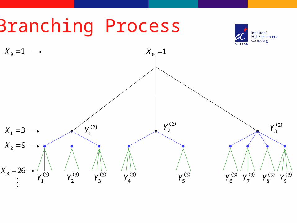
Branching Process

3 26X

1 3X

2 9X

21Y

22Y 2

3Y

31Y 3

2Y 33Y 3

5Y 34Y 3

6Y 38Y 3

7Y 39Y

0 1X 0 1X

Bienayme-Galton-Watson BP

Bienayme-Galton-Watson BP can be thought of as a stochastic model of an evolving population of particles or individuals.

It starts at time 0 with Z(0) particles, each of which splits into a random number of offspring that constitute the first generation, and so on.

The number of “offspring” produced by a single “parent” particle at any time is independent of the history of the process, and of other particles existing at the present.

The archetypal branching Process (Galton-Watson):Discrete reproduction periods (‘generations’; no overlap or parents equivalent to offspring)

1 type of individuals, with identical offspring distribution

They do not affect each other’s reproduction

Distributions of offspring numbers do not change in time

BP as an epidemic Model

Branching processes can be adopted as models for the spread of epidemic diseases.

Infections directly due to an infective are the offspring

One can approximate the infective population during the early stages of the epidemic by a branching process

Minor epidemic: Extinction of the branching processMajor epidemic: Non-extinction of the branching process

Specification & standard details

A Galton-Watson process {xn; n=0,1,2,…} is a Markov chain defined on a probability space (Ω,Γ,P) with state space Δ={0,1,…} and it has the representation

x0 = N, some specified positive integer,x1 = ξ1 + ξ2 + … + ξx0

x2 = ξx0+1 + ξx0+2 + …+ ξx0+x1...

xn = ξx0+x1+…+xn-2+1 + …+ ξx0+x1+…+xn-1

and xn = 0 if xn-1 = 0, n ≥ 1where ξi, i=1,2,… are independent and identically (iid) distributed non-negative integer valued rv on (Ω,Γ,P) and their common probability law is given by

P(ξi = k) = pk, k = 0,1,…; ∑ pk = 1

The Model

A Galton-Watson process is a Markov chain {X(n); n ≥ 0} on the non-negative integers, where for n ≥ 0

X(n+1) = ξ(n+1,1) + … ξ (n+1,X(n)) if X(n) ≥ 0 = 0 if X(n) = 0

and {ξ (n,r); r,n ≥1} are independent random variables, identically distributed like ξ (say) and with other additional assumptions. AlsoE(ξ i) = m

Offspring mean (m)

Since the offspring mean of a branching process indicates almost sure extinction or possible explosion of a population, there is considerable interest in knowing the value of this criticality parameter (growth rate parameter, basic reproductive rate)

The offspring mean (m) is also known as the infection rate and its estimation is of great interest

The problem of estimation of ‘m’ arises when we deal with the problem of determining vaccination policies aimed at preventing major epidemics

Estimation of offspring meanGalton-Watson BP is classified as:Sub-critical if m < 1 (always extinction, finite expected time to extinction)Critical if m = 1 (always extinction, infinite expected time to extinction)Super-critical if m > 1 (probability of extinction smaller than 1)

Offspring mean indicates the (almost) sure extinction or possible explosion of a population

One of the basic problems of the statistics of a G-W process is to find a ‘good’ estimator for m

Estimation methods:MLE, Least-squares, Ratio, Moment type, Bayes, etc.

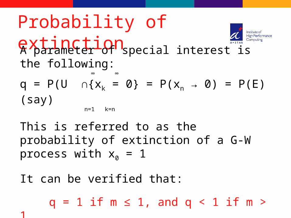
Probability of extinction

A parameter of special interest is the following: ∞ ∞

q = P(U ∩{xk = 0} = P(xn → 0) = P(E) (say) n=1 k=n

This is referred to as the probability of extinction of a G-W process with x0 = 1

It can be verified that:

q = 1 if m ≤ 1, and q < 1 if m > 1

Estimation of q is relevant when one is dealing with the recognition of a new mutation in a genetic population

Immigration Process

Estimation of the offspring mean ‘m’ breaks down in the sub-critical case ( when 0 < m < 1), in view of extinction being almost certain in such situations.

The introduction of an immigration process into the system facilitates the estimation of the offspring and immigration mean under the sub-critical case.

The analysis of a G-W process with immigration has some interesting conclusions: for example, if the mean of the offspring distribution is > 1, immigration makes very little difference to the eventual behaviour of the process.

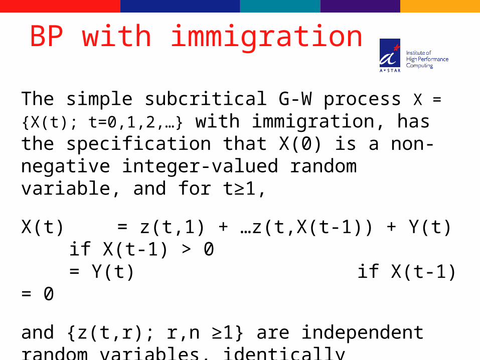
BP with immigration

The simple subcritical G-W process X = {X(t); t=0,1,2,…} with immigration, has the specification that X(0) is a non-negative integer-valued random variable, and for t≥1,

X(t) = z(t,1) + …z(t,X(t-1)) + Y(t) if X(t-1) > 0= Y(t) if X(t-1) = 0

and {z(t,r); r,n ≥1} are independent random variables, identically distributed like z (say) and with other additional assumptions.

Y(t) is the immigration component

Data Source

The data was taken from the following website:

http://sarstracker.blogspot.com/

(source: Straits Times 12 April 2003).

After careful study of the data, we transformed it into a format which could be used to fit the Galton-Watson branching process.

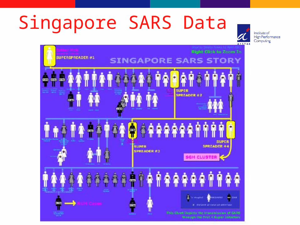
Singapore SARS Data

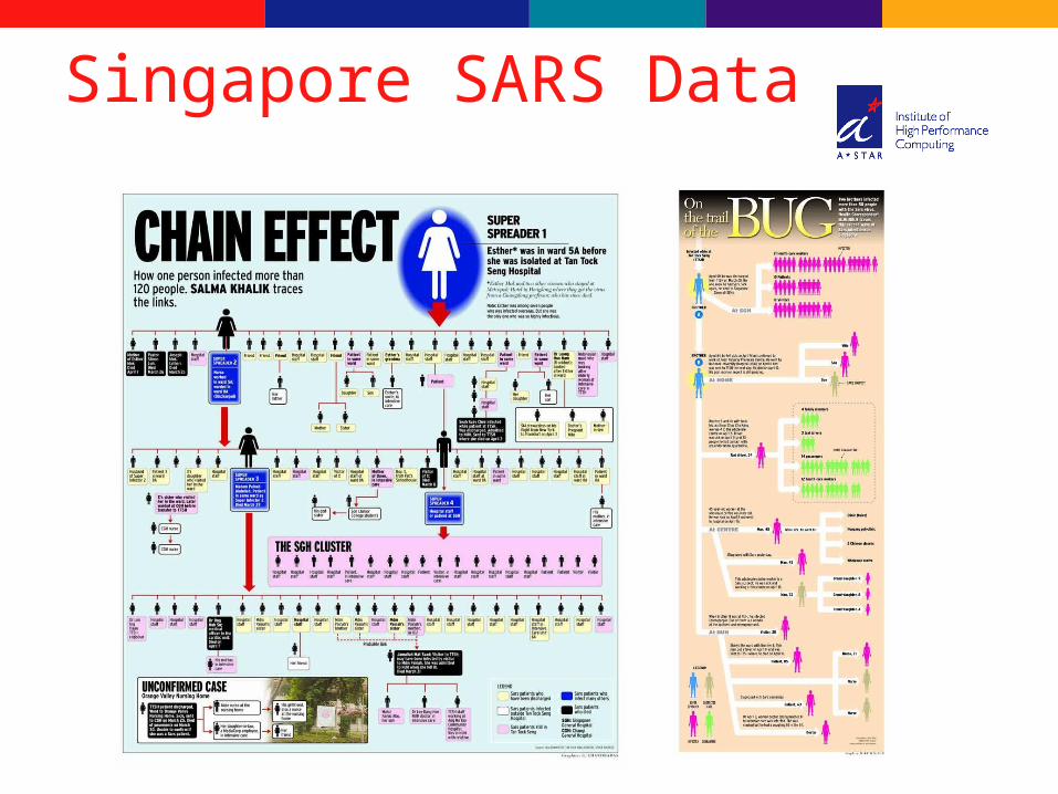
Singapore SARS Data

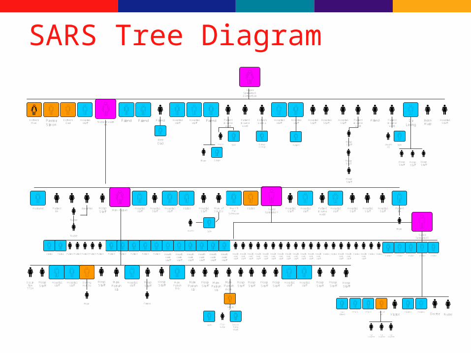
SARS Tree Diagram

HospitalStaff

SuperSpreader 1Esther Mok

Friend Patientin same

ward

IndonMaid

Patientin same

ward

HospitalStaff

DrLeong

HospitalStaff

HospitalStaff

Esther’sMom

Esther’sGrdma

Hospitalstaff

Friend Hospitalstaff

Patientin same

ward

Patientin same

ward

Friend Hospitalstaff

Hospitalstaff

FriendFriendNurse in ward5A

Hospitalstaff

PastorSimon

Esther’sDad

HerDad daughter son

Mom Sister

Esther’s Uncle

Patient

HospStaff

HospStaff

HospStaff

daughter

son

HospStaff

HospStaff

HospStaff

Husband Patient8A

daughter HospStaff

Mdm PaiinahHospital

staffHospital

StaffVisitorHospital

staffBoy 5 fr

PatSchhouse

HospitalStaff

Mom of3 in ICU

sondaughter

Visitor SuperSpreader 4

HospitalStaff

Hospitalstaff

Patientin same

ward

Hospitalstaff

HospitalStaff

HospitalStaff

HospitalStaff

Patient8A

Mom

Nurse

Nurse

Dr Limfrom

TTSH

HospStaff

Hospitalstaff

Hospitalstaff

Dr OngHok Su

Mom

HospStaff

MdmPainah

sis

Hospitalstaff

HospStaff

Friend

HospStaff

MdmPainah

Bro

MdmPainah

sis

HospStaff

MdmPainah

sis

MdmPainahmom

HospStaff

HospStaff

HospStaff

HospStaff

Hospitalstaff

Hospitalstaff

HospStaff

HospStaff

HospStaff

Heathcarestaff

Heathcarestaff

Heathcarestaff

Heathcarestaff

Heathcarestaff

Heathcarestaff

Healthcarestaff

Healthcarestaff

Healthcarestaff

Healthcarestaff

Healthcarestaff

Healthcarestaff

Healthcarestaff

Healthcarestaff

Healthcarestaff

Healthcarestaff

Healthcarestaff

Healthcarestaff

Healthcarestaff

Healthcarestaff

Healthcarestaff

Patient PatientPatient PatientPatientPatientPatientPatientPatientPatient Visitor VisitorVisitor VisitorVisitorVisitor Visitor Visitor Visitor Visitor

Jamailah

Dr LeeKang

Hoe

TTSHnurse

son

Taxidriver

PPWS PPWS PatientJamailah

GrdDaughter

GrdDaughter

GrdDaughter

VisitorPatient

Doctor Nurse

Visitor Visitor

SuperSpreader 5

MethodologyStudy the links between the SARS affected patients and identify the generation they belong to.

For example, z(0) is the initial number of patients, z(1) the next generation and so on.

Hence z(0) is the parent and z(1) is the offspring for the first generation. Similarly z(1) is the parent and z(2) is the offspring for the second generation

The parents are the infectives and the offspring the infection

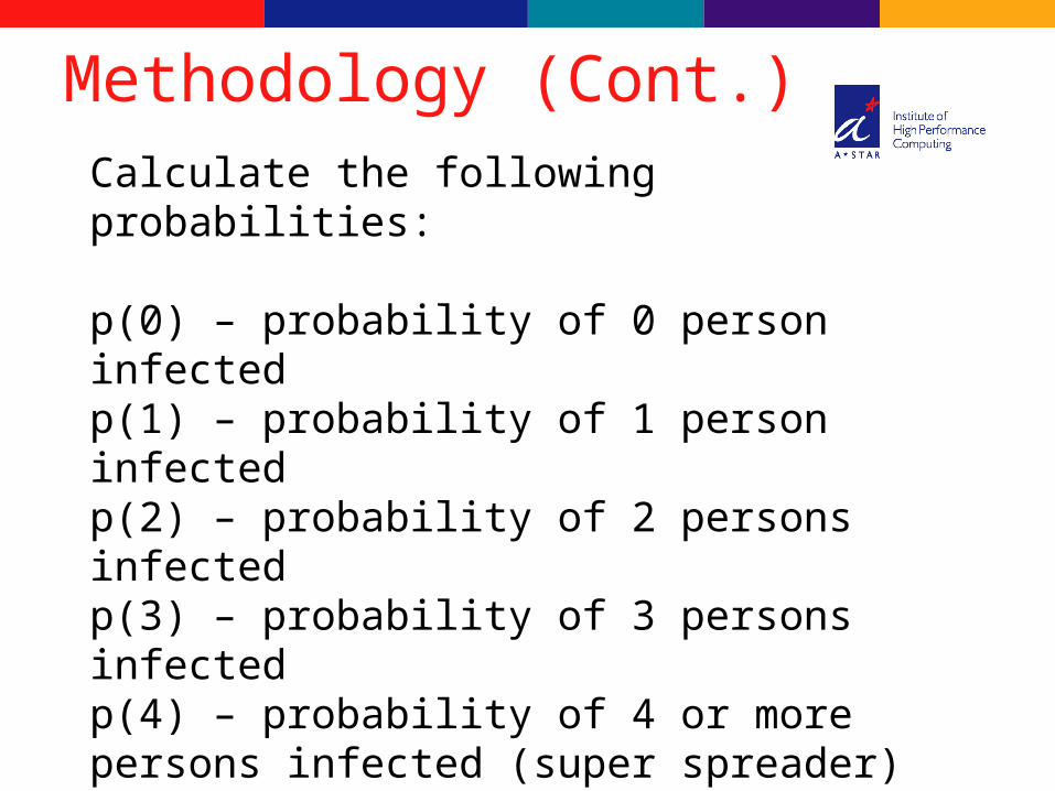
Methodology (Cont.)Calculate the following probabilities:

p(0) – probability of 0 person infected p(1) – probability of 1 person infected p(2) – probability of 2 persons infected p(3) – probability of 3 persons infected p(4) – probability of 4 or more persons infected (super spreader)

Determine the time period and fit the Galton-Watson branching process

Generation Size

Z 0 =1

     

     

     

Z 1 =25

     

     

Z 2 =36

     

     

     

Z 3 =72

     

     

     

     

Z 4 =17

     

     

     

Z 5 =6

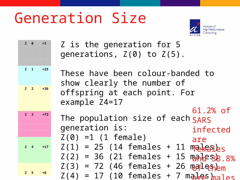
Z is the generation for 5 generations, Z(0) to Z(5).

These have been colour-banded to show clearly the number of offspring at each point. For example Z4=17

The population size of each generation is:Z(0) =1 (1 female)Z(1) = 25 (14 females + 11 males)Z(2) = 36 (21 females + 15 males)Z(3) = 72 (46 females + 26 males)Z(4) = 17 (10 females + 7 males)Z(5) = 6 (4 females + 2 males)

Total = 157 (96 females + 61 males)

61.2% of SARS infected are females and 38.8% of them are males

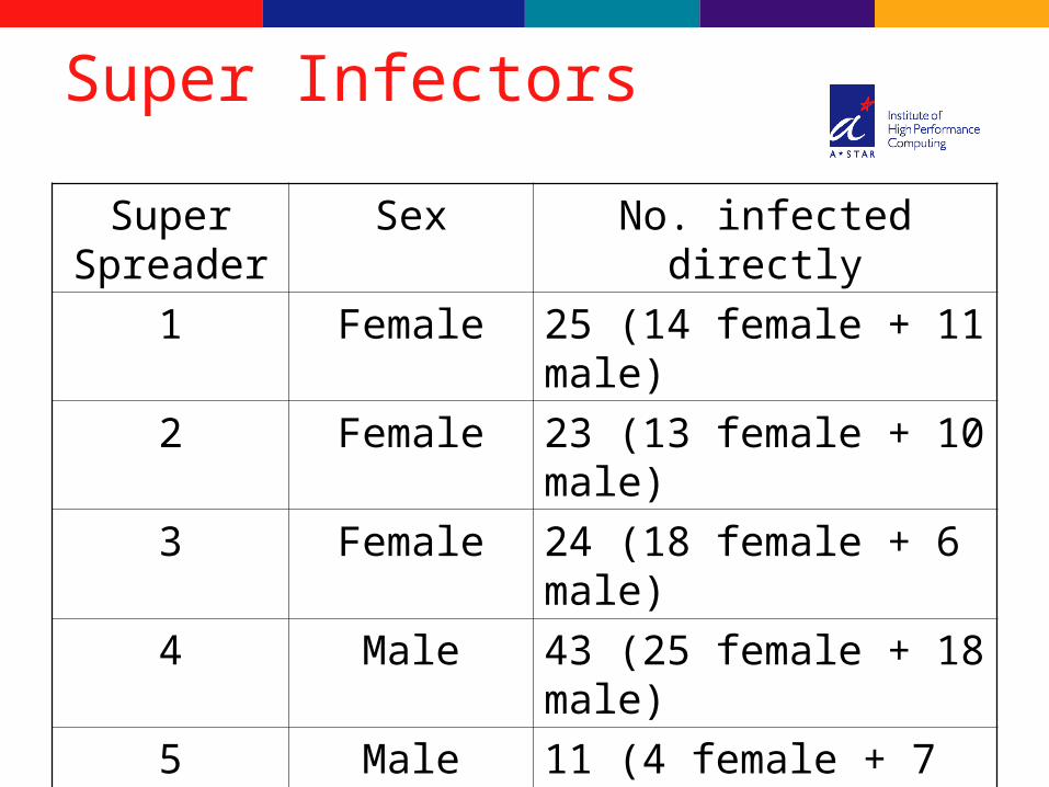
Super Infectors

Super Spreader

Sex No. infected directly

1 Female 25 (14 female + 11 male)

2 Female 23 (13 female + 10 male)

3 Female 24 (18 female + 6 male)

4 Male 43 (25 female + 18 male)

5 Male 11 (4 female + 7 male)

Probability Calculation

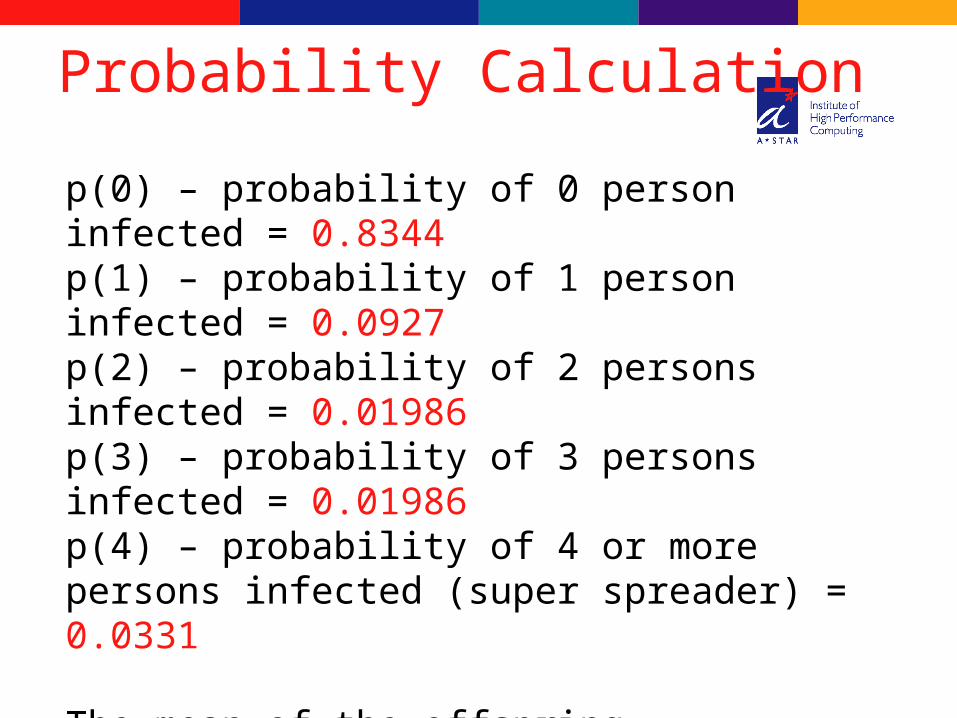
p(0) – probability of 0 person infected = 0.8344p(1) – probability of 1 person infected = 0.0927p(2) – probability of 2 persons infected = 0.01986p(3) – probability of 3 persons infected = 0.01986p(4) – probability of 4 or more persons infected (super spreader) = 0.0331

The mean of the offspring distribution is 1.0331

SoftwareTo model the SARS epidemic we use a JAVA program which simulates a single-type BP and computes the extinction probabilities.

In this program we specify the distribution for offspring in a BP and "Maximum generations" giving the number of generations we wish to observe the BP.

The program computes and displays the probabilities that the branching process will die out by generation g, for g = 1 to Maximum Generations.

Source: Written by Julian Devlin, 8/97, for the text book “Introduction to Probability”, by Charles M. Grinstead & J. Laurie Snell

Probability of extinction

Probability of Extinction of the SARS epidemic

0.75

0.8

0.85

0.9

0.95

1

1.05

1 3 5 7 9 11 13 15 17 19

Generation

Pro

bab

ilit

y

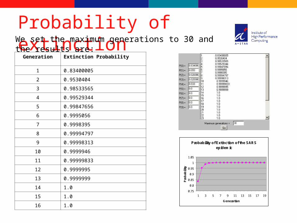
We set the maximum generations to 30 and the results are:

Generation Extinction Probability

1 0.83400005

2 0.9530404

3 0.98533565

4 0.99529344

5 0.99847656

6 0.9995056

7 0.9998395

8 0.99994797

9 0.99998313

10 0.9999946

11 0.99999833

12 0.9999995

13 0.9999999

14 1.0

15 1.0

16 1.0

Some Conclusions

The probability that the SARS epidemic will eventually become extinct is 1.

This is likely to happen in the 14th generation.Since this data has already encountered 5 generations, there can utmost be 9 more generations.

Assuming each generation takes a maximum of 10 days, based on the given data the epidemic will last only for a maximum of 90 more days from 8 April 2003.

This result is conditional upon the same environment and quarantine conditions.

Other related work @ IHPC

Auto-Regressive (AR) model

• Assumptions

Every time series data consist of both deterministic and stochastic components.

The deterministic component gives rises to trends seasonal patterns and cycles.

While the stochastic component causes statistical fluctuations which have a short term correlation structure.

Auto-Regressive (AR) model• Methodology

– Step 1: determine the maximum number of the sample data

– Step 2: calculate the mean value of the sample data for previous time

– Step 3: estimate the unknown parameters from historical data

– Step 4: use the estimated parameters to predict future case numbers

• Software

– An in-house software in FORTRAN language has been developed. It is compatible with Window systems and UNIX systems

Auto-Regressive (AR) model

0

50

100

150

200

0 10 20 30 40 50

Predicted

Observed

Two day prediction

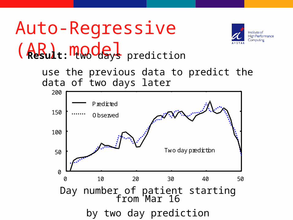
Result: two days prediction

use the previous data to predict the data of two days later

Day number of patient starting from Mar 16

by two day prediction

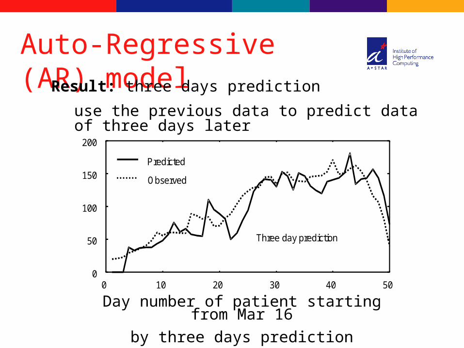
Auto-Regressive (AR) modelResult: three days prediction

use the previous data to predict data of three days later

Day number of patient starting from Mar 16

by three days prediction

0

50

100

150

200

0 10 20 30 40 50

Predicted

Observed

Three day prediction

Future Research …

A Time Series approach to the study of a Branching Process

Motivation: Venkataraman,K.N (1982) A Time Series approach to the study of the simple subcritical Galton-Watson process with immigration, Adv.Appl.Prob., 14, 1-20.

Let ε(t) = 0 for t<0; ε(0) = X(0); and for t≥1,ε(t) = X(t) – m X(t-1) – λ

Heyde and Seneta (1972) were the first to observe that the above equation is analogous to the first-order autoregressive model for time series

Vital difference: In BP ε(t) is determined by X(t) whereas in the analogous time series model X(t) will be determined in terms of ε(t)

Thank you !!!Thank you !!!