Software Engineering 3DX3

Slides 6: Stability

Dr. Ryan Leduc

Department of Computing and SoftwareMcMaster University

Material based on lecture notes by P. Taylor and M. Lawford, and Control Systems Engineering by N. Nise.

c©2006, 2007 R.J. Leduc 1

Introduction

I In this Section, we examine ways to determine if a system isstable.

I Of all design criteria, stability is most important.

I Is system is unstable, then transient response and steady-stateerror are irrelevant.

I We will now examine a few stability definitions for linear,time-invariant systems.

c©2006, 2007 R.J. Leduc 2

Stability and Natural Response

I The total response of a system is

c(t) = cforced(t) + cnatural(t)

1. A system is stable if natural response tends to zero as t →∞.

2. A system is unstable if natural response grows unbounded ast →∞.

3. A system is marginally stable if natural response neitherdecays or grows (stays constant or oscillates with fixedamplitude) as t →∞.

I Definition implies that as t →∞, only the forced responseremains.

c©2006, 2007 R.J. Leduc 3

Bounded-input, Bounded-output (BIBO) Stability

I The BIBO definition is in terms of the total response, so youdon’t need to isolate the natural response first.

1. A system is stable if every bounded input produces a boundedoutput.

2. A system is unstable if any bounded input produces anunbounded output.

c©2006, 2007 R.J. Leduc 4

Stability and Poles

I In order to easily determine if a system is stable, we canexamine the poles of the closed-loop system.

1. A system is stable if all the poles are strictly on the left handside of the complex plane.

2. A system is unstable if any pole is in the right hand side ofthe complex plane or the system has imaginary poles that areof multiplicity > 1.

3. A system is marginally stable if no pole is on the right handside, and its imaginary poles are of multiplicity one.

ie.1

(s2 + ω2)fine, but

1

(s2 + ω2)2is not.

c©2006, 2007 R.J. Leduc 5

Stability and Poles - II

I Imaginary poles of multiplicity greater than one have timeresponses of the form Atn cos(ωt + φ) which tend to infinityas t →∞.

I Implies system with imaginary poles of multiplicty one will beunstable by the BIBO definition as a sinusoid input at samefrequency (ω) will result in a total response with imaginarypoles of multiplicty two!

c©2006, 2007 R.J. Leduc 6

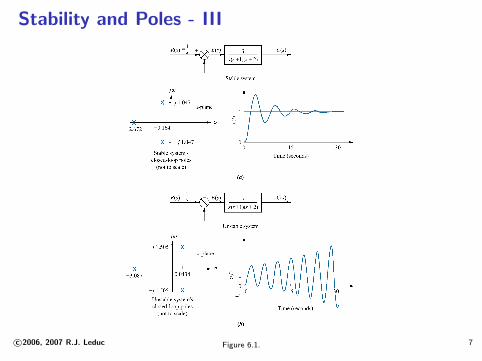
Stability and Poles - III

Figure 6.1.c©2006, 2007 R.J. Leduc 7

Stability Summary

Table: Stability Comparison

Real Part Natural BIBO

of Poles Response

All poles < 0 stable stable

Any pole > 0 or

imaginary poles of

multiplicity > 1 unstable unstable

Poles ≤ 0 marginally unstable

and imaginary poles stable

of multiplicity one

c©2006, 2007 R.J. Leduc 8

Closed-loop Systems

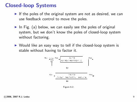
I If the poles of the original system are not as desired, we canuse feedback control to move the poles.

I In Fig. (a) below, we can easily see the poles of originalsystem, but we don’t know the poles of closed-loop systemwithout factoring.

I Would like an easy way to tell if the closed-loop system isstable without having to factor it.

Figure 6.2.

c©2006, 2007 R.J. Leduc 9

Necessary Stability Condition

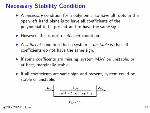
I A necessary condition for a polynomial to have all roots in theopen left hand plane is to have all coefficients of thepolynomial to be present and to have the same sign.

I However, this is not a sufficient condition.

I A sufficent condition that a system is unstable is that allcoefficients do not have the same sign.

I If some coefficents are missing, system MAY be unstable, orat best, marginally stable.

I If all coefficients are same sign and present, system could bestable or unstable.

Figure 6.3.

c©2006, 2007 R.J. Leduc 10

Routh-Hurwitz Criterion

I This method will give us stability info without having to findpoles of closed-loop system.

I Will tell us:I How many poles in left half-plane.I How many poles in right half-plane.I How many poles on imaginary axis.

I Method called Routh-Hurwitz criterion for stability.

I To apply method we need to:

1. Construct a table of data called a Routh table.2. Interpret the table to determine the above classifications.

c©2006, 2007 R.J. Leduc 11

Creating a Basic Routh Table

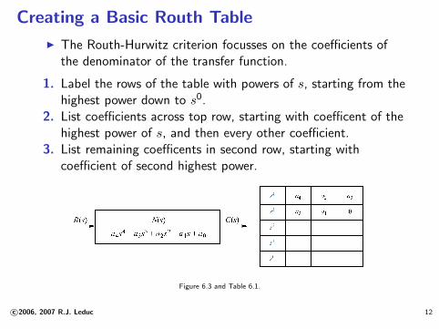
I The Routh-Hurwitz criterion focusses on the coefficients ofthe denominator of the transfer function.

1. Label the rows of the table with powers of s, starting from thehighest power down to s0.

2. List coefficients across top row, starting with coefficent of thehighest power of s, and then every other coefficient.

3. List remaining coefficents in second row, starting withcoefficient of second highest power.

Figure 6.3 and Table 6.1.

c©2006, 2007 R.J. Leduc 12

Creating a Basic Routh Table - II

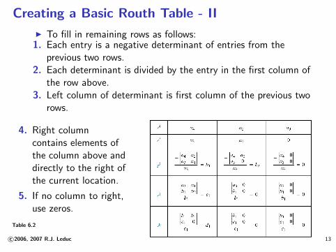
I To fill in remaining rows as follows:1. Each entry is a negative determinant of entries from the

previous two rows.2. Each determinant is divided by the entry in the first column of

the row above.3. Left column of determinant is first column of the previous two

rows.

4. Right columncontains elements ofthe column above anddirectly to the right ofthe current location.

5. If no column to right,use zeros.

Table 6.2

c©2006, 2007 R.J. Leduc 13

Interpreting a Basic Routh Table

I Basic Routh table applies to systems with poles in open left orright hand plane, but no imaginary poles.

I The Routh-Hurwitz criterion states that the number of polesin the right half plane is equal to the number of sign changesin the first coefficient column of the table.

I A system is stable if there are no sign changes in the firstcolumn.

c©2006, 2007 R.J. Leduc 14

Basic Routh Table eg.

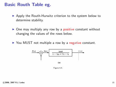
I Apply the Routh-Hurwitz criterion to the system below todetermine stability.

I One may multiply any row by a positive constant withoutchanging the values of the rows below.

I You MUST not multiple a row by a negative constant.

Figure 6.4.

c©2006, 2007 R.J. Leduc 15

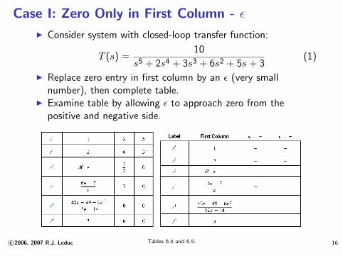
Case I: Zero Only in First Column - ε

I Consider system with closed-loop transfer function:

T (s) =10

s5 + 2s4 + 3s3 + 6s2 + 5s + 3(1)

I Replace zero entry in first column by an ε (very smallnumber), then complete table.

I Examine table by allowing ε to approach zero from thepositive and negative side.

Tables 6.4 and 6.5.c©2006, 2007 R.J. Leduc 16

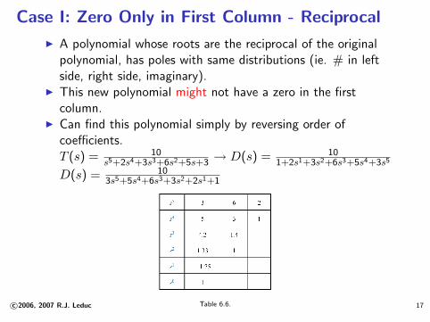
Case I: Zero Only in First Column - Reciprocal

I A polynomial whose roots are the reciprocal of the originalpolynomial, has poles with same distributions (ie. # in leftside, right side, imaginary).

I This new polynomial might not have a zero in the firstcolumn.

I Can find this polynomial simply by reversing order ofcoefficients.T (s) = 10

s5+2s4+3s3+6s2+5s+3→ D(s) = 10

1+2s1+3s2+6s3+5s4+3s5

D(s) = 103s5+5s4+6s3+3s2+2s1+1

Table 6.6.c©2006, 2007 R.J. Leduc 17

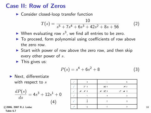
Case II: Row of ZerosI Consider closed-loop transfer function

T (s) =10

s5 + 7s4 + 6s3 + 42s2 + 8s + 56(2)

I When evaluating row s3, we find all entries to be zero.I To proceed, form polynomial using coefficients of row above

the zero row.I Start with power of row above the zero row, and then skip

every other power of s.I This gives us:

P (s) = s4 + 6s2 + 8 (3)

I Next, differentiatewith respect to s

dP (s)

ds= 4s3 + 12s1 + 0

(4)

Table 6.7

c©2006, 2007 R.J. Leduc 18

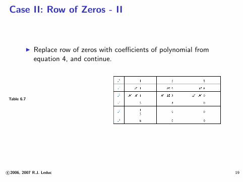
Case II: Row of Zeros - II

I Replace row of zeros with coefficients of polynomial fromequation 4, and continue.

Table 6.7

c©2006, 2007 R.J. Leduc 19

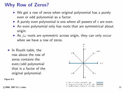
Why Row of Zeros?

I We get a row of zeros when original polynomial has a purelyeven or odd polynomial as a factor.

I A purely even polynomial is one where all powers of s are even.I An even polynomial only has roots that are symmetrical about

origin.I As jω roots are symmetric across origin, they can only occur

when we have a row of zeros.

I In Routh table, therow above the row ofzeros contains theeven/odd polynomialthat is a factor of theoriginal polynomial.

Figure 6.5

c©2006, 2007 R.J. Leduc 20

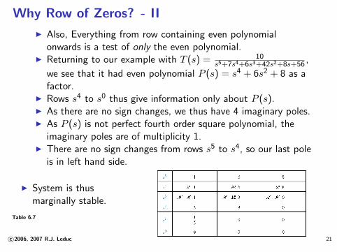
Why Row of Zeros? - II

I Also, Everything from row containing even polynomialonwards is a test of only the even polynomial.

I Returning to our example with T (s) = 10s5+7s4+6s3+42s2+8s+56

,

we see that it had even polynomial P (s) = s4 + 6s2 + 8 as afactor.

I Rows s4 to s0 thus give information only about P (s).I As there are no sign changes, we thus have 4 imaginary poles.I As P (s) is not perfect fourth order square polynomial, the

imaginary poles are of multiplicity 1.I There are no sign changes from rows s5 to s4, so our last pole

is in left hand side.

I System is thusmarginally stable.

Table 6.7

c©2006, 2007 R.J. Leduc 21

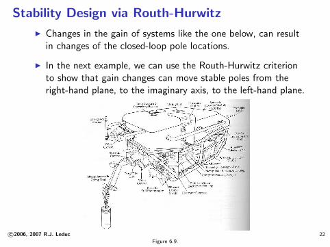
Stability Design via Routh-Hurwitz

I Changes in the gain of systems like the one below, can resultin changes of the closed-loop pole locations.

I In the next example, we can use the Routh-Hurwitz criterionto show that gain changes can move stable poles from theright-hand plane, to the imaginary axis, to the left-hand plane.

Figure 6.9.

c©2006, 2007 R.J. Leduc 22

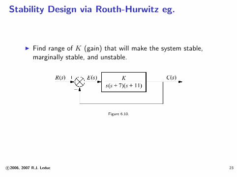
Stability Design via Routh-Hurwitz eg.

I Find range of K (gain) that will make the system stable,marginally stable, and unstable.

Figure 6.10.

c©2006, 2007 R.J. Leduc 23

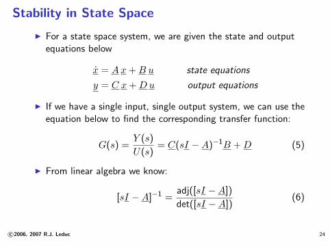
Stability in State Space

I For a state space system, we are given the state and outputequations below

x = A x + B u state equations

y = C x + D u output equations

I If we have a single input, single output system, we can use theequation below to find the corresponding transfer function:

G(s) =Y (s)

U(s)= C(sI −A)−1B + D (5)

I From linear algebra we know:

[sI −A]−1 =adj([sI −A])

det([sI −A])(6)

c©2006, 2007 R.J. Leduc 24

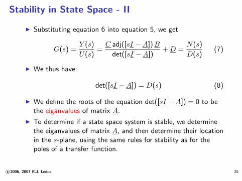
Stability in State Space - II

I Substituting equation 6 into equation 5, we get

G(s) =Y (s)

U(s)=

C adj([sI −A])B

det([sI −A])+ D =

N(s)

D(s)(7)

I We thus have:

det([sI −A]) = D(s) (8)

I We define the roots of the equation det([sI −A]) = 0 to bethe eiganvalues of matrix A.

I To determine if a state space system is stable, we determinethe eiganvalues of matrix A, and then determine their locationin the s-plane, using the same rules for stability as for thepoles of a transfer function.

c©2006, 2007 R.J. Leduc 25