Embed Size (px)
Citation preview
Air Force Institute of Technology Air Force Institute of Technology
AFIT Scholar AFIT Scholar
Theses and Dissertations Student Graduate Works
3-2001
Solar Radiation Pressure Modeling Issues for High Altitude Solar Radiation Pressure Modeling Issues for High Altitude
Satellites Satellites
Dayne G. Cook
Follow this and additional works at: https://scholar.afit.edu/etd
Part of the Astrodynamics Commons
Recommended Citation Recommended Citation Cook, Dayne G., "Solar Radiation Pressure Modeling Issues for High Altitude Satellites" (2001). Theses and Dissertations. 4591. https://scholar.afit.edu/etd/4591
This Thesis is brought to you for free and open access by the Student Graduate Works at AFIT Scholar. It has been accepted for inclusion in Theses and Dissertations by an authorized administrator of AFIT Scholar. For more information, please contact [email protected].
SOLAR RADIATION PRESSURE MODELING ISSUES FOR
HIGH ALTITUDE SATELLITES
THESIS
Dayne G. Cook, Major, USAF
AFIT/GSO/ENY/01M-01
DEPARTMENT OF THE AIR FORCE AIR UNIVERSITY
AIR FORCE INSTITUTE OF TECHNOLOGY Wright-Patterson Air Force Base, Ohio
APPROVED FOR PUBLIC RELEASE; DISTRIBUTION UNLIMITED
20010523 025
The views expressed in this thesis axe those of the author and do not reflect the
official policy or position of the United States Air Force, Department of Defense, or
the U.S. Government.
AFIT/GSO/ENY/OlM-01
SOLAR RADIATION PRESSURE MODELING ISSUES FOR
HIGH ALTITUDE SATELLITES
THESIS
Presented to the Faculty
Department of Aeronautics and Astronautics
Graduate School of Engineering and Management
Air Force Institute of Technology
Air University
Air Education and Training Command
in Partial Fulfillment of the Requirements for the
Degree of Master of Science in Space Operations
Dayne G. Cook, B.S.
Major, USAF
March 2001
APPROVED FOR PUBLIC RELEASE; DISTRIBUTION UNLIMITED
AFIT/GSO/ENY/OlM-01
SOLAR RADIATION PRESSURE MODELING ISSUES FOR
HIGH ALTITUDE SATELLITES
Dayne G. Cook, B.S. Major, USAF
Approved:
* rtAkOi ßtlAr^n\ JO (AA^^ Steven G. Tragesser Date Committee Chair ^ , -
William E. Wiesel Date Committee Member
Gregory S. Agnes Date Committee Member
Acknowledgements
I would be remiss in my duties as a student if I did not thank all those who
have taught me. My sincere appreciation goes to my AFIT instructors, all of whom
played a role in helping me reach this end state. Out in front of all these, I am truly
indebted to my thesis advisor, Dr. Steven Tragesser, for keeping me on the straight
and narrow path. I thank you for all your assistance, mentoring, and continual
guidance in re-vectoring my efforts when I went astray.
This experience would not have been possible without the camaraderie and
constant bolstering of good friends. Thanks to Don Davis, Charles Galbreath and
Jack Oldenburg for your encouragement and support. Special thanks also to those
behind the scenes; administration, EN laboratory staff, and all other support per-
sonnel who make it possible for us to function as graduate students.
I express heartfelt gratitude to my Heavenly Father from whom which all bless-
ings flow. To my parents, I thank you for everything you have taught me and for
your earnest prayers and words of inspiration when I needed them most. Last but
not least, I thank my loving wife, without whom I would never have made it through
this ordeal. To you I express my sincere love and appreciation for your enduring
patience and understanding.
Dayne G. Cook
IV
Table of Contents
Page
Acknowledgements iv
List of Figures vii
List of Tables ix
List of Symbols x
List of Abbreviations xiv
Abstract xv
I. Introduction 1-1
1.1 Motivation 1-1
1.2 Background 1-2
1.2.1 Orbit Perturbations and Solar Radiation Pressure 1-2
1.2.2 Simplified General Perturbation Model .... 1-4
1.3 Problem Statement 1-4
1.4 Research Objectives 1-5
II. Previous Research 2-1
2.1 Early 2-1
2.2 Contemporary 2-3
III. Methodology 3-1
3.1 Perturbation Techniques 3-1
3.2 Models 3-4
3.2.1 Baseline 3-4
Page
3.2.2 Changing Area 3-16
3.2.3 Diffuse Reflection 3-19
3.2.4 Changing Area Revisited 3-27
3.2.5 Conical Eclipse 3-38
3.3 Coordinate Transformations 3-44
3.4 Calculating and Optimizing Residuals 3-49
IV. Results 4-1
4.1 Numerical Examples 4-1
4.2 Baseline Behavior 4-2
4.2.1 IUS in GTO 4-2
4.2.2 DSP in GEO 4-5
4.2.3 Orbital Elements Long-term Periodic Variations 4-9
4.3 Changing Area 4-13
4.4 Diffuse Reflection 4-15
4.5 Conical Eclipse 4-16
4.6 Constant Solar Flux 4-17
V. Conclusion 5-1
5.1 Summary and Recommendations 5-1
5.2 Future Work 5-2
Appendix A. SRP Model FORTRAN Source Code A-l
A.l Simulation Algorithm for SRP Study A-l
A.2 JPL Planetary and Lunar Ephemerides A-21
Bibliography BIB-1
Vita VITA-1
VI
List of Figures Figure Page
2.1. Early Method for Measuring Radiation Pressure 2-1
3.1. Flat Plate Geometry 3-8
3.2. Specular Reflection 3-9
3.3. Isotropie Solar Radiation 3-11
3.4. Cylindrical Earth Shadow Model 3-13
3.5. Differential Area Projection to the Sun 3-16
3.6. Solar Force Geometry 3-17
3.7. Diffuse Reflection 3-20
3.8. Diffuse Ray Geometry 3-21
3.9. Hemisphere Integration 3-23
3.10. Earth-Satellite-Sun Vector Geometry 3-27
3.11. Cylinder (IUS) Body-Frame Geometry 3-29
3.12. Cylinder (IUS) Ends Illumination Geometry 3-33
3.13. DSP Body-Frame Geometry 3-36
3.14. Conical Earth Shadow Model 3-39
3.15. Angular Radius 3-40
3.16. No Eclipse 3-41
3.17. Umbral Eclipse 3-42
3.18. Penumbral Eclipse 3-43
3.19. Inertial to Body-Frame Transformation 3-45
3.20. IUS Body-Frame and Orbital Geometry 3-47
3.21. DSP Body-Frame and Orbital Geometry 3-48
4.1. SRP Baseline Behavior for IUS Semi-major Axis 4-2
4.2. SRP Baseline Behavior for IUS Eccentricity 4-3
Vll
Figure Page
4.3. SRP Baseline Behavior for IUS Inclination 4-4
4.4. SRP Baseline Behavior for IUS Argument of Perigee 4-4
4.5. SRP Baseline Behavior for IUS RAAN 4-5
4.6. SRP Baseline Behavior for DSP Semi-major Axis 4-6
4.7. SRP Baseline Behavior for DSP Eccentricity 4-7
4.8. SRP Baseline Behavior for DSP Inclination 4-7
4.9. SRP Baseline Behavior for DSP Argument of Perigee 4-8
4.10. SRP Baseline Behavior for DSP RAAN 4-8
4.11. SRP Effects on Long-term Variations of Eccentricity 4-9
vin
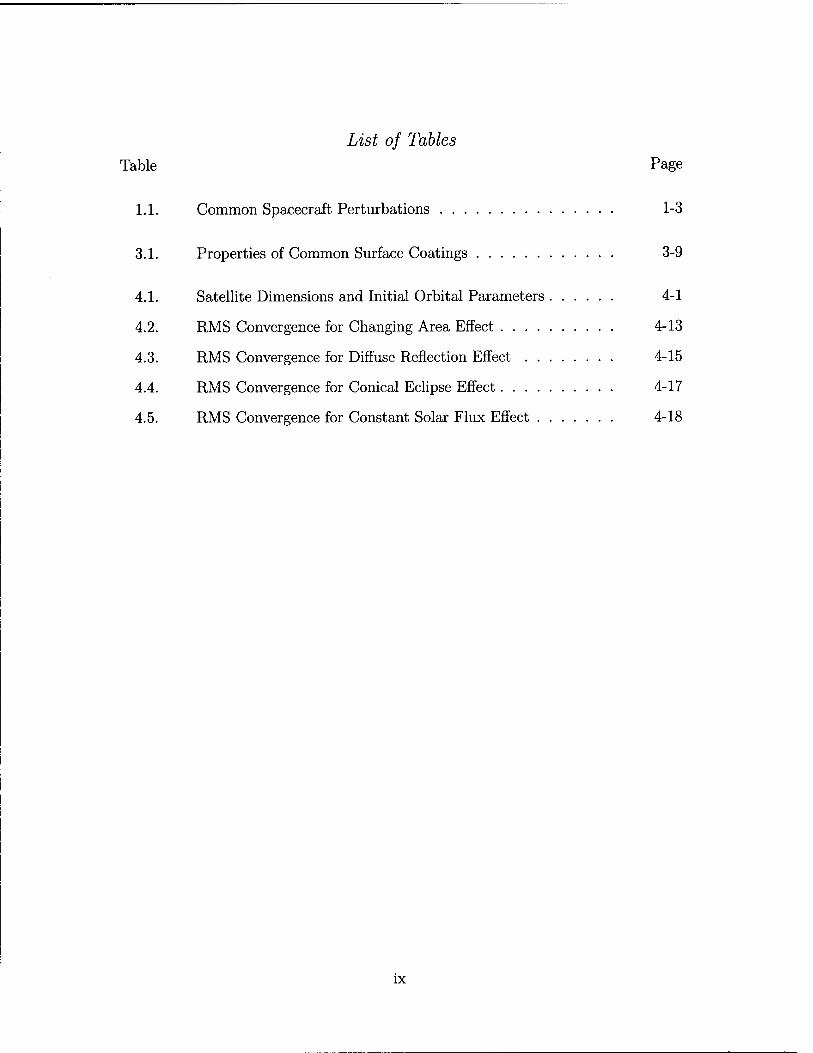
List of Tables Table Page
1.1. Common Spacecraft Perturbations 1-3
3.1. Properties of Common Surface Coatings 3-9
4.1. Satellite Dimensions and Initial Orbital Parameters 4-1
4.2. RMS Convergence for Changing Area Effect 4-13
4.3. RMS Convergence for Diffuse Reflection Effect 4-15
4.4. RMS Convergence for Conical Eclipse Effect 4-17
4.5. RMS Convergence for Constant Solar Flux Effect 4-18
IX
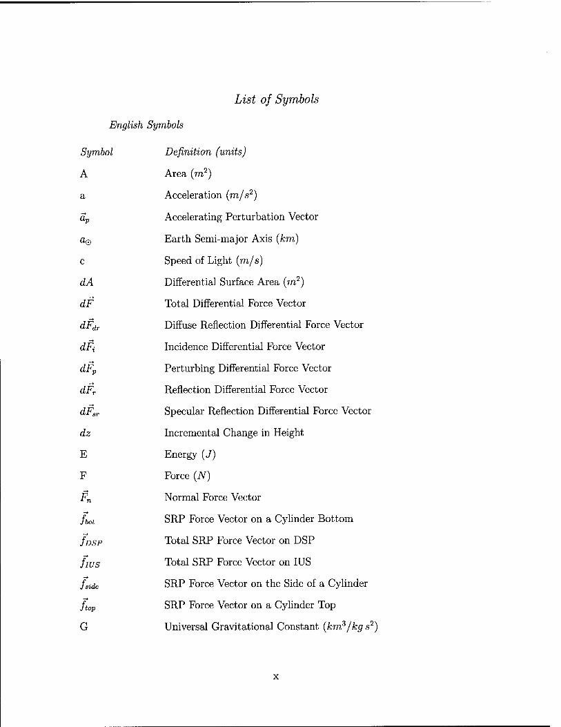
List of Symbols
English Symbols
Symbol Definition (units)
A Area (m2)
a Acceleration (m/s2)
ap Accelerating Perturbation Vector
a0 Earth Semi-major Axis (km)
c Speed of Light (m/s)
dA Differential Surface Area (ra2)
dF Total Differential Force Vector
dFdr Diffuse Reflection Differential Force Vector —*
dFi Incidence Differential Force Vector
dFp Perturbing Differential Force Vector
dFr Reflection Differential Force Vector
dFsr Specular Reflection Differential Force Vector
dz Incremental Change in Height
E Energy (J)
F Force (N)
Fn Normal Force Vector
fbot SRP Force Vector on a Cylinder Bottom
fDSP Total SRP Force Vector on DSP
fws Total SRP Force Vector on IUS
fside SRP Force Vector on the Side of a Cylinder
ftop SRP Force Vector on a Cylinder Top
G Universal Gravitational Constant (km3/kg s2)
x
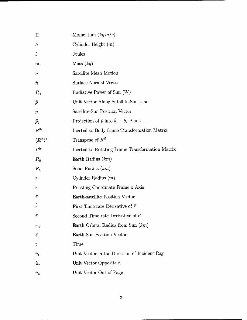
H Momentum (kg m/s)
h Cylinder Height (m)
J Joules
m Mass (kg)
n Satellite Mean Motion
h Surface Normal Vector
Pe Radiative Power of Sun (W)
P Unit Vector Along Satellite-Sun Line
P Satellite-Sun Position Vector
Pi Projection of p into bi — b2 Plane
Rib Inertial to Body-frame Transformation Matrix
(Rib)T Transpose of R11
Rir Inertial to Rotating Frame Transformation Matrix
R® Earth Radius (km)
RQ Solar Radius (km)
r Cylinder Radius (TO)
f Rotating Coordinate Frame x Axis
r Earth-satellite Position Vector
f First Time-rate Derivative of r
f Second Time-rate Derivative of f
r& Earth Orbital Radius from Sun (km)
s Earth-Sun Position Vector
t Time
Ui Unit Vector in the Direction of Incident Ray
Un Unit Vector Opposite h
U0 Unit Vector Out of Page
XI
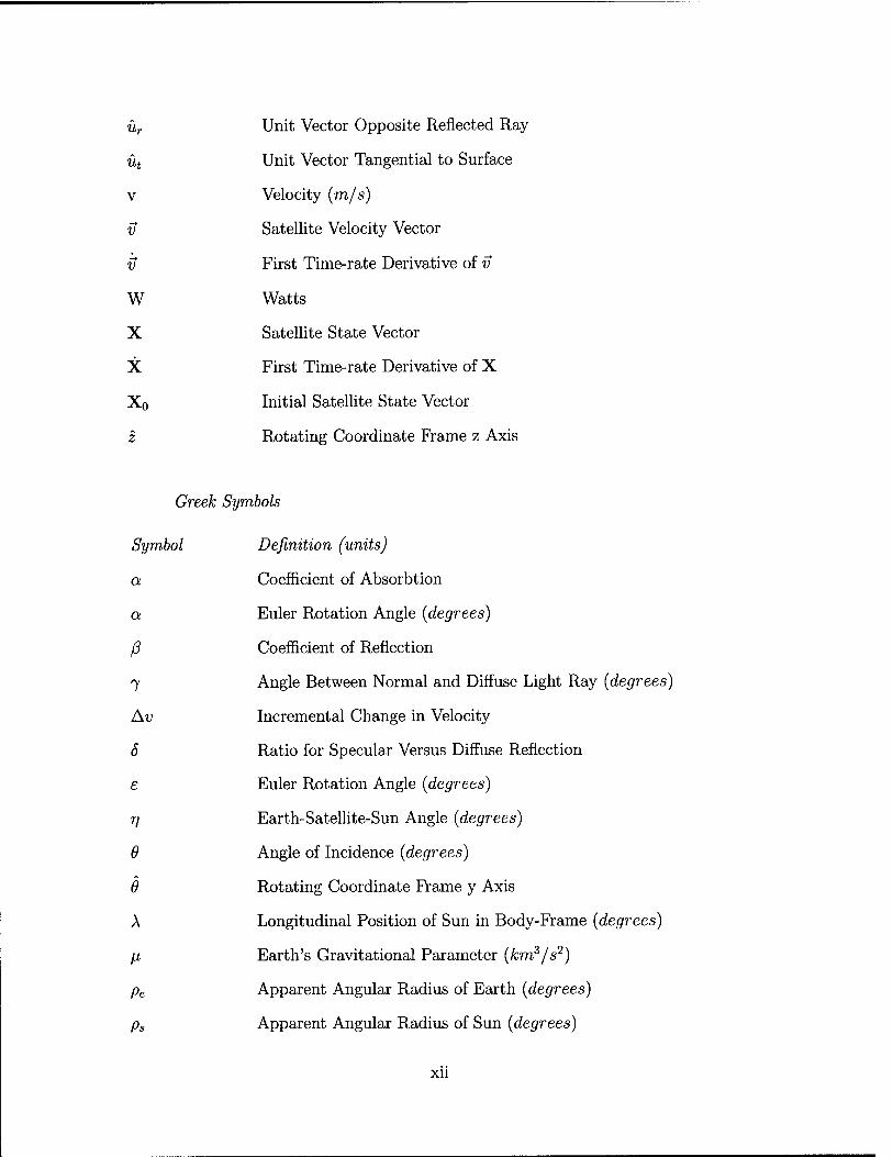
ür Unit Vector Opposite Reflected Ray
ut Unit Vector Tangential to Surface
v Velocity (m/s)
v Satellite Velocity Vector
v First Time-rate Derivative of v
W Watts
X Satellite State Vector
X First Time-rate Derivative of X
Xo Initial Satellite State Vector
z Rotating Coordinate Frame z Axis
Greek Symbols
Symbol Definition (units)
a Coefficient of Absorbtion
a Euler Rotation Angle (degrees)
ß Coefficient of Reflection
7 Angle Between Normal and Diffuse Light Ray (degrees)
Av Incremental Change in Velocity
5 Ratio for Specular Versus Diffuse Reflection
e Euler Rotation Angle (degrees)
T) Earth-Satellite-Sun Angle (degrees)
6 Angle of Incidence (degrees)
6 Rotating Coordinate Frame y Axis
A Longitudinal Position of Sun in Body-Frame (degrees)
// Earth's Gravitational Parameter (km3/s2)
pe Apparent Angular Radius of Earth (degrees)
ps Apparent Angular Radius of Sun (degrees)
xii
T Fraction of Solar Disk Visible from Satellite
$ Solar Flux (W/m2)
$0 Solar Flux Constant (W/m2)
(j) Azimuthal Angle (degrees)
tp Sun-Earth-satellite Angle (degrees)
Q Rotational Spin Rate (rad/s)
xin
Abbreviation
AFRL
AU
DSP
DSST
ECI
GEO
GPS
GTO
IUS
JPL
NASA
NORAD
OD
RAAN
RMS
rpm
SGP
SI
SRP
TDRSS
List of Abbreviations
Definition
Air Force Research Laboratory
Astronomical Unit
Defense Support Program
Draper Semianalytic Satellite Theory
Earth Centered Inertial
Geosynchronous Earth Orbit
Global Positioning Satellite
Geosynchronous Transfer Orbit
Inertial Upper Stage
Jet Propulsion Laboratory
National Aeronautics and Space Administration
North American Aerospace Defense
Orbit Determination
Right Ascension of Ascending Node
Root Mean Square
Revolutions per Minute
Simplified General Perturbation
System International
Solar Radiation Pressure
Tracking and Data Relay Satellite System
xiv
AFIT/GSO/ENY/OlM-01
Abstract
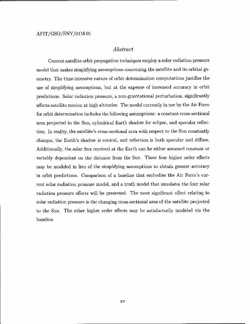
Current satellite orbit propagation techniques employ a solar radiation pressure
model that makes simplifying assumptions concerning the satellite and its orbital ge-
ometry. The time-intensive nature of orbit determination computations justifies the
use of simplifying assumptions, but at the expense of increased accuracy in orbit
predictions. Solar radiation pressure, a non-gravitational perturbation, significantly
affects satellite motion at high altitudes. The model currently in use by the Air Force
for orbit determination includes the following assumptions: a constant cross-sectional
area projected to the Sun, cylindrical Earth shadow for eclipse, and specular reflec-
tion. In reality, the satellite's cross-sectional area with respect to the Sun constantly
changes, the Earth's shadow is conical, and reflection is both specular and diffuse.
Additionally, the solar flux received at the Earth can be either assumed constant or
variably dependent on the distance from the Sun. These four higher order effects
may be modeled in lieu of the simplifying assumptions to obtain greater accuracy
in orbit predictions. Comparison of a baseline that embodies the Air Force's cur-
rent solar radiation pressure model, and a truth model that simulates the four solar
radiation pressure effects will be presented. The most significant effect relating to
solar radiation pressure is the changing cross-sectional area of the satellite projected
to the Sun. The other higher order effects may be satisfactorily modeled via the
baseline.
xv
SOLAR RADIATION PRESSURE MODELING ISSUES FOR
HIGH ALTITUDE SATELLITES
/. Introduction
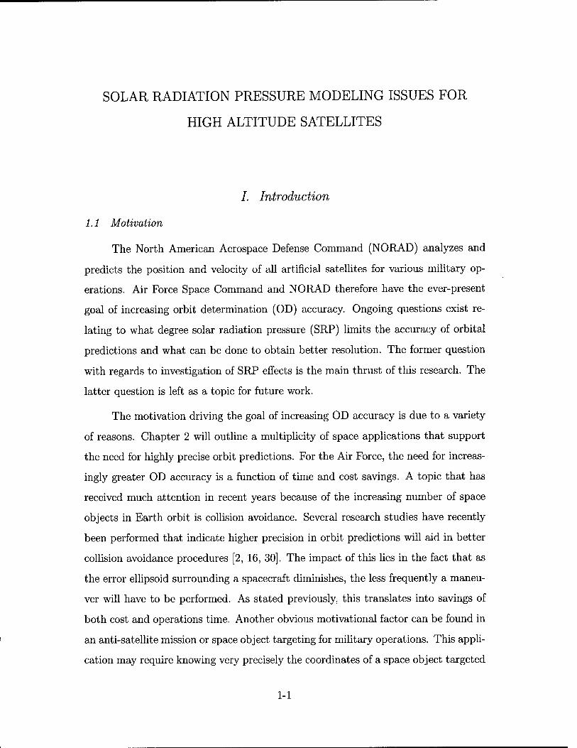
1.1 Motivation
The North American Aerospace Defense Command (NORAD) analyzes and
predicts the position and velocity of all artificial satellites for various military op-
erations. Air Force Space Command and NORAD therefore have the ever-present
goal of increasing orbit determination (OD) accuracy. Ongoing questions exist re-
lating to what degree solar radiation pressure (SRP) limits the accuracy of orbital
predictions and what can be done to obtain better resolution. The former question
with regards to investigation of SRP effects is the main thrust of this research. The
latter question is left as a topic for future work.
The motivation driving the goal of increasing OD accuracy is due to a variety
of reasons. Chapter 2 will outline a multiplicity of space applications that support
the need for highly precise orbit predictions. For the Air Force, the need for increas-
ingly greater OD accuracy is a function of time and cost savings. A topic that has
received much attention in recent years because of the increasing number of space
objects in Earth orbit is collision avoidance. Several research studies have recently
been performed that indicate higher precision in orbit predictions will aid in better
collision avoidance procedures [2, 16, 30]. The impact of this lies in the fact that as
the error ellipsoid surrounding a spacecraft diminishes, the less frequently a maneu-
ver will have to be performed. As stated previously, this translates into savings of
both cost and operations time. Another obvious motivational factor can be found in
an anti-satellite mission or space object targeting for military operations. This appli-
cation may require knowing very precisely the coordinates of a space object targeted
1-1
for either offensive or defensive operations. For these reasons, SRP is an extremely
important factor in modeling the various perturbations acting upon a satellite and
should not be hastily disregarded.
1.2 Background
1.2.1 Orbit Perturbations and Solar Radiation Pressure. All objects in
space experience external forces that influence and characterize their motion. The
primary force acting on an Earth-orbiting satellite is the gravitational attraction
that results if all of the Earth's mass is assumed to occupy a uniform density sphere.
Influences such as Earth's uneven mass distribution, gravitational attraction of ad-
ditional Solar System bodies, atmospheric drag, solar radiation pressure, Earth's
albedo, and other relatively small forces perturb the satellite away from the natural
two-body motion. For this reason, these types of forces are called perturbations.
SRP is the impingement of light energy (photons) on an object's surface and is
responsible for the subsequent exchange of momentum. Table 1.1 lists the common
perturbations acting upon a satellite orbiting the Earth and gives a general idea of
where SRP fits within the range of other force magnitudes [23]. In Table 1.1, A/M
is the ratio of the satellite's area to its mass. Assuming an A/M of 0.01 m2/kg, the
magnitude of SRP acceleration is approximately 4.6 x 10~8 m/s2. The formula for
SRP given in Table 1.1, indicates that an increase in satellite area or a decrease in
satellite mass, will result in an amplified SRP value.
Orbital perturbations may be classified as either gravitational or non-gravitational.
The first four perturbations in Table 1.1 are gravitational and the last three, includ-
ing SRP, are non-gravitational. Note the absence of the Universal Gravitational
Constant term, G, in the formulas for these perturbations. It is evident in Table
1.1 that the gravitational perturbations are dominant for near-Earth orbit. How-
ever, depending on the precision and accuracy required in orbit determination under
specified conditions, non-gravitational perturbations may have a significant effect on
the satellite.
1-2
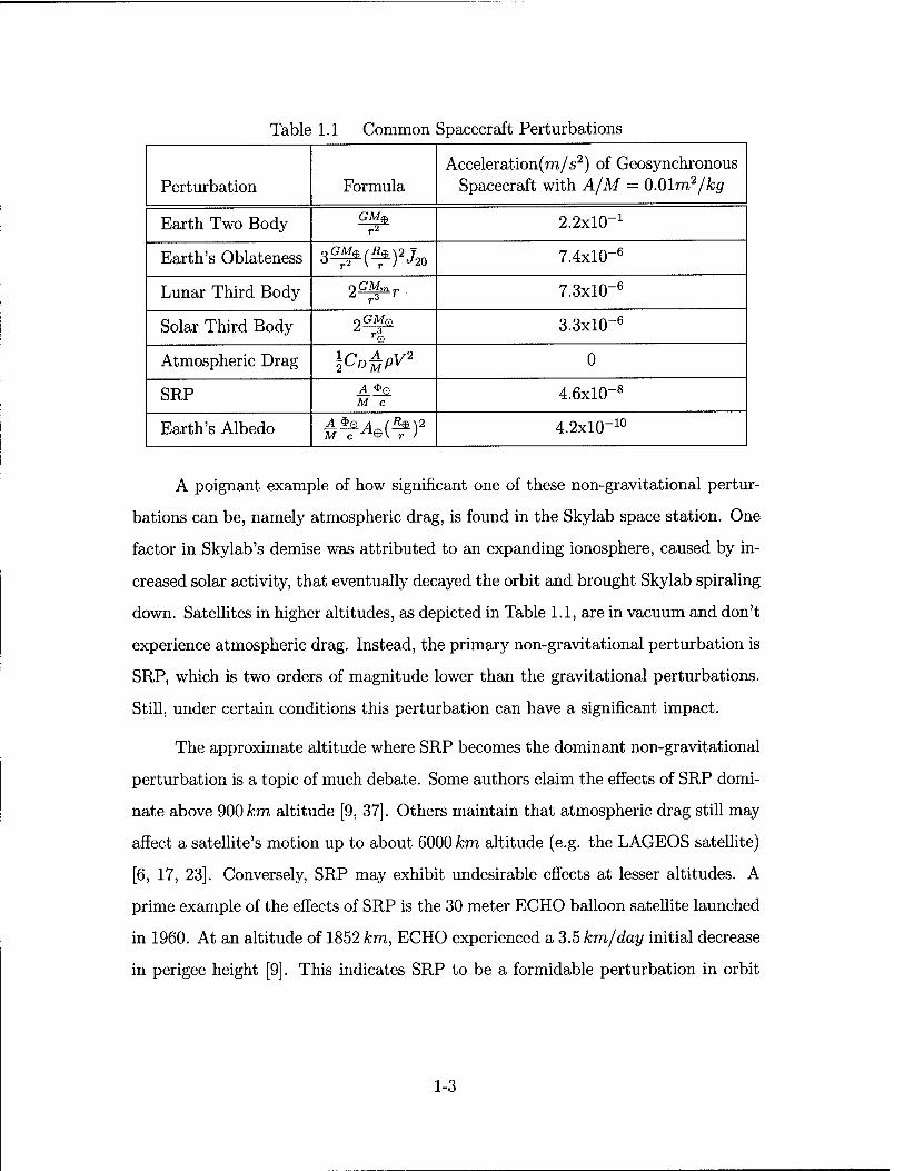
Table 1.1 Common Spacecraft Perturbations
Perturbation Formula Acceleration(ra/s2) of Geosynchronous
Spacecraft with A/M = 0.01m2/kg
Earth Two Body GM9 r2 2.2XKT1
Earth's Oblateness 3^(^)2J20 7.4xl0~6
Lunar Third Body r,GMm r3 7.3xl0-6
Solar Third Body r,GMe 2 r%
3.3xl0~6
Atmospheric Drag pD+pV* 0
SRP A £©_ M c 4.6xl(T8
Earth's Albedo M c ^©V r ) 4.2xl0"10
A poignant example of how significant one of these non-gravitational pertur-
bations can be, namely atmospheric drag, is found in the Skylab space station. One
factor in Skylab's demise was attributed to an expanding ionosphere, caused by in-
creased solar activity, that eventually decayed the orbit and brought Skylab spiraling
down. Satellites in higher altitudes, as depicted in Table 1.1, are in vacuum and don't
experience atmospheric drag. Instead, the primary non-gravitational perturbation is
SRP, which is two orders of magnitude lower than the gravitational perturbations.
Still, under certain conditions this perturbation can have a significant impact.
The approximate altitude where SRP becomes the dominant non-gravitational
perturbation is a topic of much debate. Some authors claim the effects of SRP domi-
nate above 900 km altitude [9, 37]. Others maintain that atmospheric drag still may
affect a satellite's motion up to about 6000 km altitude (e.g. the LAGEOS satellite)
[6, 17, 23]. Conversely, SRP may exhibit undesirable effects at lesser altitudes. A
prime example of the effects of SRP is the 30 meter ECHO balloon satellite launched
in 1960. At an altitude of 1852 km, ECHO experienced a 3.5 km/day initial decrease
in perigee height [9]. This indicates SRP to be a formidable perturbation in orbit
1-3
determination. The challenge then becomes to sufficiently model SRP effects on
satellites in order to accurately make predictions of their motion.
1.2.2 Simplified General Perturbation Model. Given the perturbations that
may influence a satellite's motion, a model is required which accounts for these effects
and accurately propagates the satellite's orbit. One such model used by NORAD in
tracking space objects is the Simplified General Perturbation (SGP) model [24].
Orbital models can be grouped into one of two computational classifications:
numerical and analytical. The former method entails a step-by-step numerical in-
tegration in time of the equations of motion, including any perturbations affecting
the satellite. This method requires pre-determined initial conditions of the satellite's
position and velocity in order to propagate to the desired point in time. The latter
method involves an analytical solution that directly computes the satellite's position
and velocity at a specified time. Numerical integration produces highly accurate
predictions, but requires substantial computation time since the satellite's position
and velocity must be calculated at each time step of the integration.
NORAD is responsible for tracking and cataloging high volumes of objects
in space. The computationally time-prohibitive nature of numerical integration led
NORAD to develop a fully analytical model in the 1970s called SGP. The SGP model
required NORAD to make some simplifying assumptions relating to low satellite
orbital eccentricity and negligible satellite mass compared to the Earth's mass [17].
Over time, the growing number of Earth orbiting satellites became more complex
in both orbital geometry and physical design. In an effort to reap the benefits of
both computational methods, NORAD refined their SGP model. The result is the
semi-analytical SGP4 model currently used by NORAD [24].
1.3 Problem Statement
The SRP acceleration in NORAD's SGP4 model, which is approxiamtely 20
years old, incorporates several simplifying assumptions [24]. The satellite orbit is
1-4
propagated assuming a constant cross-sectional area projected to the Sun, a cylin-
drical Earth shadow for eclipse, and specular reflection. As with any simplifying
assumption made for the sake of computational ease and efficiency, these assump-
tions do not reflect the true state of the environment. The satellite's projected
cross-sectional area with respect to the Sun constantly changes over the course of
one orbital revolution, as well as throughout the course of a year. The Earth's
shadow is actually conical in shape and includes two distinct regions. Reflection
off the satellite's surface is both specular and diffuse. These factors cause the SRP
acceleration to fluctuate in time and results in imprecise orbit predictions if not
modeled properly. Furthermore, the SRP perturbation can result in long-term pe-
riodic oscillations in perigee altitude as well as in eccentricity and semi-major axis
of the orbit. Since gravitational perturbations have been modeled quite carefully in
SGP4, improvements to the SRP model, a non-gravitational perturbation, should
improve OD accuracy. The question this research will address is, how beneficial is it
to employ a complex model that accounts for the SRP higher order effects.
1.4 Research Objectives
The objective of this research is to model the effects of SRP in an orbit per-
turbations model. This goal will be realized through the quantification of modeling
errors in order to determine which higher order aspects of SRP must be incorporated
in the OD process. SRP acceleration varies throughout the satellite's orbit as orbital
characteristics and satellite attitude change. The reasons the SRP acceleration may
fluctuate are the antithesis of the simplifying assumptions identified in Section 1.3,
and hence include:
1. Changes in the satellite cross-sectional area incident to the Sun.
2. Time periods when the satellite is in conical eclipse behind the Earth.
3. Specular versus diffuse reflection off the satellite's surface.
These higher order modeling effects will comprise the bulk of the research analysis
and will be simulated via a computer algorithm. How advantageous modeling these
1-5
higher order SRP effects can be, hinges on the required accuracy of orbit predictions,
motivation of which was presented in the previous section.
Accomplishment of the research objectives will follow a straightforward pro-
gression. The previous research outlined in the next chapter gives a firm foundation
for developing the SRP acceleration model and its higher order effects. Each re-
search effort cited makes contribution to how SRP can more effectively be modeled.
Chapter 3 will discuss the methodology utilized in the development of a SRP model,
including simplifying assumptions and higher order effects. Chapter 4 will illustrate
and numerically quantify results derived from simulation of the model to be devel-
oped in Chapter 3. Chapter 5 will then formulate recommendations and summarize
any conclusions as well as address the subject of future work.
1-6
77. Previous Research
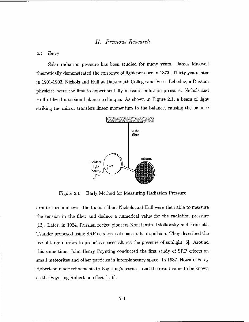
2.1 Early
Solar radiation pressure has been studied for many years. James Maxwell
theoretically demonstrated the existence of light pressure in 1873. Thirty years later
in 1901-1903, Nichols and Hull at Dartmouth College and Peter Lebedev, a Russian
physicist, were the first to experimentally measure radiation pressure. Nichols and
Hull utilized a torsion balance technique. As shown in Figure 2.1, a beam of light
striking the mirror transfers linear momentum to the balance, causing the balance
torsion fiber
mirrors
1
Figure 2.1 Early Method for Measuring Radiation Pressure
arm to turn and twist the torsion fiber. Nichols and Hull were then able to measure
the tension in the fiber and deduce a numerical value for the radiation pressure
[13]. Later, in 1924, Russian rocket pioneers Konstantin Tsiolkovsky and Fridrickh
Tsander proposed using SRP as a form of spacecraft propulsion. They described the
use of large mirrors to propel a spacecraft via the pressure of sunlight [5]. Around
this same time, John Henry Poynting conducted the first study of SRP effects on
small meteorites and other particles in interplanetary space. In 1937, Howard Percy
Robertson made refinements to Poynting's research and the result came to be known
as the Poynting-Robertson effect [1, 9].
2-1
With the advent of the Space Age, SRP became an increasingly important
consideration in precise orbit determination. The effects of SRP on the orbits of
Earth satellites first caught the attention of researchers and space enthusiasts in the
early 1960's. The launch and subsequent perturbations of the Vanguard and ECHO
satellites prompted early researchers to develop models that would suitably account
for SRP effects. Some of these early authors include Musen, Kozai and Koskela
[18, 27]. One thing these authors all had in common was their use of simplifying
assumptions as alluded to in the previous chapter. Namely, these authors assumed
constant cross-sectional area, cylindrical Earth Shadow, and specular reflection, as
well as constant solar flux [18]. The model that these authors describe, minus the
assumption concerning constant solar flux, will be elaborated upon as a baseline
model in Section 3.2.1. Subsequent research began to alter and refine these simplify-
ing assumptions in varying degrees, thereby building up a more complicated but also
more precise model for SRP. The model to be developed in Chapter 3 will consider
each of these effects and explore their impact on SRP acceleration.
The National Aeronautics and Space Administration (NASA) also expressed
concern on the subject of SRP early on in the Space Age. Robert Bryant of the
Goddard Space Flight Center conducted a study on SRP effects for NASA in 1961.
Bryant observed that in the absence of Earth shadow, SRP effects provided only short
periodic terms in the semi-major axis of the orbit. It was only when the obscuring
effect of the Earth was included that SRP manifested a significant perturbation [7].
This observation was later verified by others, the import of which is that the long-
term effects of SRP on the orbit are greater when the satellite encounters eclipsing
of the Sun [27]. Since Bryant's work took place prior to the advent of the modern
computer, his research focused on developing a system of equations for the osculating
orbital elements, that could then be integrated on a large scale computer mainframe
[7].
2-2
2.2 Contemporary
Since the time Bryant conducted his study, satellites have evolved into highly
complex systems with widely varying missions and orbital characteristics. This has
prompted a number of research endeavors to study the various aspects of SRP un-
der diverse conditions. With regards to satellite shape, the most simple model is
that of a spherically symmetric satellite, resulting in a constant cross-sectional area
and acceleration vector along the Sun-satellite line. One such model is examined
by Harwood et al. who use Lagrange equations to solve for the variations in the
orbital elements [14]. As with other models, simplifying assumptions were made for
computational efficiency. Assumptions include a cylindrical Earth shadow and Sun-
satellite vector parallel to the Sun-Earth vector. Additionally, the Earth's distance
from the Sun is allowed to vary in this model, thereby causing the solar flux value to
oscillate and produce a time-varying SRP acceleration. Chapter 3 will discuss how
these assumptions may be refined to achieve more precise SRP calculations.
A more complex modeling effort by Marshall et al. discusses the need for very
precise orbital computations of an oceanographic satellite called TOPEX/Poseidon
[22]. This satellite takes altimeter measurements from which the ocean topography
is mapped. Precise modeling of SRP is justified in this case because even minute
inaccuracies in orbit determination can translate into major discrepancies in topo-
graphical measurements. The required accuracy in these measurements stipulate
orbit predictions within 13 cm root-mean-square (RMS) precision in the radial com-
ponent over a 10-day orbit fit span. The authors assumed a box-wing satellite model
consisting of six flat plates arranged as a box and an additional flat plate for the
solar panel. The cross-sectional area projected by each plate was allowed to change
according to predefined attitude and orbital dynamics. Force components on each
plate were computed individually and then summed to get the total vector accelera-
tion. Other assumptions in this model include a cylindrical Earth shadow, Lambert's
cosine law for diffuse reflection, and constant surface reflective properties. These ba-
sic assumptions will also be applied to the model described in Chapter 3. There is
2-3
one other item of notable mention within Marshall's model. Even though SRP was
assumed to be the primary non-gravitational force, complementary effects due to the
Earth's albedo and infrared emissions, as well as satellite thermal emissions, were
also included in order to obtain the most accurate predictions possible.
TOPEX/Poseidon is not the only satellite system that requires extremely ac-
curate orbit predictions. The Global Positioning Satellite (GPS) is responsible for
providing timely and accurate global navigational data to military, civilian, and com-
mercial agencies. It has been shown that the largest error source for a GPS orbit is
due to the effects of SRP. Springer et al. have recently developed a new SRP model
for GPS that outperforms the previous model derived without SRP effects by an
order of magnitude [31]. The new model consists of a 6-element parameterization
of direct solar radiation terms and biases that define the acceleration as a result of
SRP. The residual RMS of this new model on a 7-day orbit fit came in at the 6 cm
level, an improvement of 69 cm over the model that lacked any SRP effects. As this
model demonstrates, careful attention to how SRP is modeled can have impressive
results in the orbit analysis. It must be emphasized however, that while the 13 cm
RMS of the TOPEX/Poseidon and the 6 cm RMS of the GPS appear to be rather
amazing, their fit spans are over relatively short periods of time. The secular effects
of SRP seem to suggest that it might make more sense to perform the analysis over
a longer time period, in order to obtain a broader perspective of SRP effects. To
this end, it is the intention of the model presented in the next chapter to simulate
over a period of one year.
The previous examples of SRP research were of spacecraft in orbit about the
Earth. SRP however affects all objects in interplanetary space to some degree or an-
other. A Japanese project named SELENE, currently underway for a lunar mission
in 2003, is studying the long-term effects of SRP on a relay satellite in orbit about
the Moon [19]. Since the Moon has no atmosphere to speak of, SRP is the most
dominant non-gravitational perturbation acting on the satellite. The force equation
used in this model is consistent with that used by Chobotov [8], Ries et al. [27],
2-4
and Milani et al. [23] and will be explicitly derived in Chapter 3. The satellite
shape is that of an octagonal column, and as such is modeled as a combination of
flat plates much like TOPEX/Poseidon. It is interesting to note that this project
supports Bryant's research [7], in that no long-term variation in semi-major axis of
the satellite's orbit is evident in the absence of shadow. This is due to the model as-
sumption that shadowing by the Moon is neglected. The model does however exhibit
variations in other orbital elements, primarily eccentricity [19]. These conclusions
will be demonstrated further in Chapter 4.
Other research efforts have focused on the generalities of perturbation model-
ing. Researchers at the Charles Stark Draper Laboratory have developed a mean
element orbit propagator called the Draper Semianalytic Satellite Theory (DSST).
The DSST model allows a user to tailor force modeling options depending on the
desired accuracy and duration of computation time. This method, reminiscent of the
NORAD SGP4 model, incorporates the high speed of a general perturbations model
and the superior accuracy found in a special perturbations model. DSST assumes
a cylindrical Earth shadow and constant coefficient of reflection for its SRP model.
The Air Force Research Laboratory (AFRL) astrodynamics group has successfully
employed DSST since 1994 [28]. The model developed in Chapter 3 of this thesis is of
the special perturbations type, and as such will place greater emphasis on accuracy
than computational time.
The AFRL further articulated interest with regards to SRP in a 1998 report
by Luu and Sabol [21]. With the use of DSST, the authors applied pre-defined
assumptions to the SRP model in order to determine the overall effects on space
debris in supersynchronous orbit. The design interface of DSST allowed the authors
to define input parameters based on the nature of the orbital characteristics of this
particular scenario, which were the basis for their simplifying assumptions. One of
these assumptions was that an object in circular supersynchronous orbit is constantly
sunlit. While this is not completely accurate, the authors justify this assumption
by showing that the long-periodic variations in semi-major axis are at the submeter
2-5
level and therefore negligible for their purposes. However, SRP-induced variations
in eccentricity and argument of perigee are still significant for objects above Geosyn-
chronous Earth Orbit (GEO) and still require inclusion in the model. The variation
in eccentricity over a six-month period may fluctuate from 0.001 to 0.004 in this
case. A similar conclusion regarding the long-periodic variations in semi-major axis,
eccentricity, and argument of perigee over a period of one year will be illustrated in
Chapter 4.
Another non-gravitational perturbation study by Bowman et al. illustrates the
detrimental long-term effects of SRP, atmospheric drag, and Earth albedo [6]. In
1963, one of the first concepts of space communications was realized with the launch
of the West Ford needles package. The idea was to place a myriad of copper dipoles,
1.78 cm long and 0.00178 cm in diameter, in a circular, near-polar orbit at an altitude
of 3650 km. These dipole antennas were intended to relay communications signals
around the country. The orbits of individual needles all decayed within 5 years of
launch. Sixty percent of the needle clusters still remain in orbit and have been tracked
for the past 37 years with rising difficulty. The needle clusters exhibit a large area-to-
mass ratio, which has made them susceptible to the non-gravitational perturbations
mentioned above. Recall in Table 1.1 that a larger area-to-mass ratio (A/M) implies
an increased magnitude in non-gravitational perturbations. The result for the West
Ford needle clusters has been a total displacement of 10 km in the semi-major axis
over the past 34 years. The effects of a varying area-to-mass ratio as related to SRP
will be explored in Chapter 3.
One of the other time-varying factors affecting SRP is the shadowing effect of
Earth eclipses. Up to this point, all previously cited research has assumed either an
Earth cylindrical shadow or has neglected shadowing effects completely. In reality,
the shadow of the Earth is conical in shape and includes both a penumbra and umbra
region. Recall that the consequence of not accurately modeling shadow effects is
diminished precision in predicting long-term variations of the orbit semi-major axis
2-6
[7, 19]. The portent of this conclusion has led some researchers to scrutinize the
shadow model in greater detail.
Vokrouhlicky et al. have written a series of papers on the complete theory
of spacecraft eclipse transition [33, 34, 35, 36]. A similar paper by J. Woodburn
discusses the effects of eclipse boundary crossing on numerical integration [39]. The
supposition in these papers is that the Earth projects a conical shadow with two dis-
tinct shadow regions, penumbra and umbra. As a spacecraft transits the penumbra
region, the perceived size of the solar disk by the spacecraft changes. This transition
determines the fluctuating value of solar intensity, which in turn affects the magni-
tude of SRP [1]. Another item of related interest in Vokrouhlicky's work, but not
considered hereafter in this thesis, is the inclusion of influences on the Earth shadow
structure due to atmospheric density and flattening of the Earth's pole [36]. Various
aspects of the Earth shadow model will be investigated in greater detail in Section
3.2.5 and results given in Chapter 4.
Heretofore, previous SRP research examples have focused on exploiting only
some of the SRP effects mentioned in Section 1.4, but none of them have attempted
to combine all effects at once. There is one research study however that comes close
to nullifying all these basic simplifying assumptions. NASA's Tracking and Data
Relay Satellite System (TDRSS) is a GEO system used for command and tracking
support of user spacecraft. Previously, TDRSS was modeled as a uniform sphere
with constant area for modeling nonconservative forces, including SRP. The model
for TDRSS has since been improved in order to achieve more precise orbit predictions
[20].
TDRSS is now modeled as a combination of twenty-four flat plates, each with
its own radiation force. These individual vector forces are then summed to obtain the
resultant acceleration acting on the spacecraft. The changing area projected by these
flat plates, as perceived by the Sun, is determined by a geometrically defined angle
of incidence. This then nullifies the assumption concerning constant area. Next, the
2-7
new model assumes an Earth umbra/penumbra model versus the cylindrical shadow
model so frequently used before [20]. With regards to surface reflective properties, an
elemental surface behaves as a linear combination of a black body, a perfect mirror
and a Lambert diffuser [23]. This means the model accounts for both specular and
diffuse reflection, and is consistent with the SRP model articulated by Chobotov [8]
and Milani [23]. The authors of this study cite a constant value for the solar radiation
flux, wherein lies the only difference between this model and the one developed in
the next chapter. As will be shown, it is a simple matter to account for the changing
solar radiation flux as a function of distance from the Sun.
2-8
III. Methodology
3.1 Perturbation Techniques
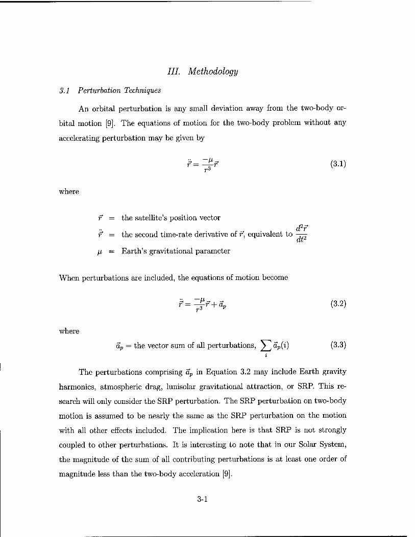
An orbital perturbation is any small deviation away from the two-body or-
bital motion [9]. The equations of motion for the two-body problem without any
accelerating perturbation may be given by
?= =£r (3.i)
where
r = the satellite's position vector
f = the second time-rate derivative of r, equivalent to -—^
H = Earth's gravitational parameter
When perturbations are included, the equations of motion become
f=^tf+ap (3.2)
where
ap = the vector sum of all perturbations, V^ap(i) (3.3) i
The perturbations comprising ap in Equation 3.2 may include Earth gravity
harmonics, atmospheric drag, lunisolar gravitational attraction, or SRP. This re-
search will only consider the SRP perturbation. The SRP perturbation on two-body
motion is assumed to be nearly the same as the SRP perturbation on the motion
with all other effects included. The implication here is that SRP is not strongly
coupled to other perturbations. It is interesting to note that in our Solar System,
the magnitude of the sum of all contributing perturbations is at least one order of
magnitude less than the two-body acceleration [9].
3-1
There are two existing categories of perturbation technique that may be used to
solve Equation 3.2. The two techniques are called special perturbations and general
perturbations. The former technique involves a step-by-step numerical integration of
the equations of motion. General perturbations is an analytical approach based on
a series expansion and integration of the equations of variation in orbit parameters
[3, 9]. As mentioned in Chapter 2, the perturbation technique utilized in this research
is of the special perturbations type.
The special perturbations technique may further be partitioned into two main
methods. CowelPs method was developed by P.H. Cowell in the early 20th cen-
tury and is the most straightforward of the perturbation techniques. Some fifty
years earlier in 1857, Johann Franz Encke formulated Encke's method for solving
perturbations, albeit more complex in nature. The difference lies in the fact that
Cowell's method performs numerical integration on the sum of all accelerations,
whereas Encke's method takes the difference between the primary acceleration and
the perturbing accelerations prior to integrating [3]. The method employed in the
derivation found in this chapter is Cowell's method. Additionally, the Runge-Kutta
method for numerical integration will be used in the computer simulation.
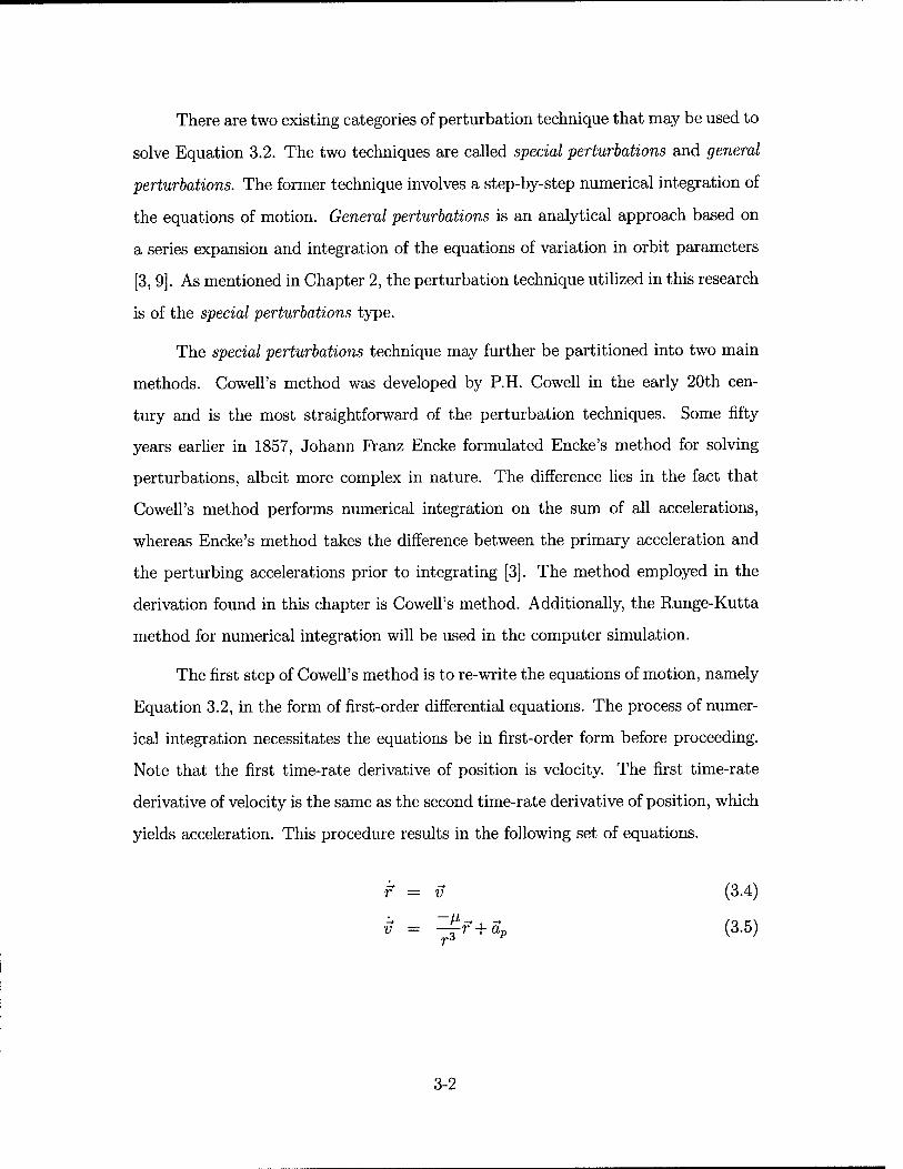
The first step of Cowell's method is to re-write the equations of motion, namely
Equation 3.2, in the form of first-order differential equations. The process of numer-
ical integration necessitates the equations be in first-order form before proceeding.
Note that the first time-rate derivative of position is velocity. The first time-rate
derivative of velocity is the same as the second time-rate derivative of position, which
yields acceleration. This procedure results in the following set of equations.
f = v (3.4)
v = —r + äp (3.5)
3-2
where
r = first time-rate derivative of the satellite position vector
v = satellite velocity vector
v = first time-rate derivative of the satellite velocity vector
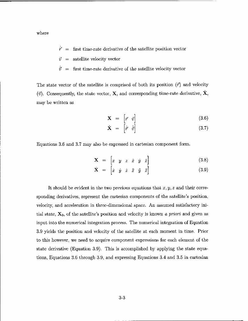
The state vector of the satellite is comprised of both its position (r) and velocity
(v). Consequently, the state vector, X, and corresponding time-rate derivative, X,
may be written as
X =
X =
r v
f v
(3.6)
(3.7)
Equations 3.6 and 3.7 may also be expressed in cartesian component form.
X =
X =
x y z x y z
x y z x y z
(3.8)
(3.9)
It should be evident in the two previous equations that x, y, z and their corre-
sponding derivatives, represent the cartesian components of the satellite's position,
velocity, and acceleration in three-dimensional space. An assumed satisfactory ini-
tial state, X0, of the satellite's position and velocity is known a priori and given as
input into the numerical integration process. The numerical integration of Equation
3.9 yields the position and velocity of the satellite at each moment in time. Prior
to this however, we need to acquire component expressions for each element of the
state derivative (Equation 3.9). This is accomplished by applying the state equa-
tions, Equations 3.6 through 3.9, and expressing Equations 3.4 and 3.5 in cartesian
3-3
component form.
X = X(4)
y = X(5)
z = X(6)
= ~ßX 1 a X (a;2 +2,2 + ^2)3/2 ' aP*
= ~ßV 1 a y (£2 + ^2+3.2)3/2 ' aPV
= ~ßZ 1 a z (x2 + y2 + x2f/2 pz (3.10)
These six equations therefore comprise the first-order differential equations
suitable for numerical integration, the result of which will be predictions of satellite
position and velocity. Given satisfactory initial conditions, the first three formulas
in Equation 3.10 are ready for integration. The remaining formulas however require
further derivation. The ap components found in these formulas represent the accel-
erating perturbation due to SRP. The derivation of the ap components are the focus
of the remainder of this chapter.
3.2 Models
3.2.1 Baseline. The baseline model presented here will be used as a ref-
erence model from which the other effects of SRP may be quantitatively analyzed.
The baseline model will be represented by the SRP model found in NORAD's SGP4
model, which obeys the previously made assumptions [24]:
1. Cross-sectional area incident to the Sun remains constant.
2. Earth cylindrical shadow for satellite in eclipse.
3. Reflection from the satellite's surface is specular.
The derivation of the baseline model begins with the investigation of photon
energy. Photons impinging on a satellite's surface follow the electromagnetic mass-
3-4
energy relationship given by
E = mc2 (3.11)
where
E = photon energy (J)
m = photon mass (kg)
c = speed of light (m/s)
If we divide both sides of Equation 3.11 by c, we get
E — = mc c
(3.12)
Note that the product mc is an increment of momentum, a product of mass and
velocity, and may be re-written as
- = AH (3.13) c
where A if is the change in momentum. The average rate of solar energy received
at the Earth is given by the solar flux constant, $0, and is expressed in units of
W/m2. Energy (E) may now be re-defined as the product of solar flux incident on a
given area and over a specified duration. We can thus substitute this definition into
Equation 3.13 to obtain
5^ = AH (3.14) c
where
A = sunlit surface area of satellite (m2)
At = time interval of sunlight exposure (s)
3-5
Dividing both sides by At yields
$0A _ AH (3.15)
Setting Equation 3.15 aside for the time being, we now consider the force resulting
from the impinging photons. Newton's second law states that the force experienced
by an object is proportional to the time-rate change of its momentum. Mathemati-
cally, this is most commonly expressed as
F = ma (3.16)
where
m = mass of satellite (kg)
a = acceleration of satellite (m/s2)
Replacing the product ma in Equation 3.16 with its time-rate derivative form gives
F=jt (mv) (3.17)
where ^ (mv) is now the time-rate derivative of momentum. This equation applies
to electromagnetic radiation if we substitute the momentum of the photon, H, for
the product mv.
F=df (3.18)
Since we are not interested in this equation in differential form, we can replace the
differential operator with standard A nomenclature.
A ff F==r- (3-19) At v '
3-6
We can now substitute the right-hand side of this equation from Equation 3.15 to
get
F = ^ (3.20) c
We can also substitute the left-hand side of this equation from Equation 3.16 and
obtain
ma = (o.zlj c
Isolate acceleration by now dividing through by mass.
a = *± (3.22) c m
Comparing this equation to the formula for SRP found in Table 1.1, we find that they
are identical. In spite of this, Equation 3.22 is not yet entirely complete. Note that
acceleration is a vector and Equation 3.22 gives only the scalar value. The remaining
elements for this equation include a vector direction for acceleration, a coefficient that
determines how efficient the surface is in reflecting incident radiation, and a scaling
factor to account for the changing solar flux.
One of the previously made simplifying assumptions for the baseline model
is that the cross-sectional area of the satellite facing the Sun remains constant.
Therefore, the satellite shape may be modeled as either a sphere with equivalent
constant area or a flat plate with fixed orientation normal to the Sun. For illustration
purposes, it is easiest to show the case of a flat plate. Figure 3.1 depicts the solar
force geometry on a flat plate with constant area normal to the Sun. Incident light
strikes the flat plate at a perpendicular angle. Reflected light leaves the satellite
along the surface normal vector, n. The resultant force vector, Fn, as well as the
corresponding acceleration vector, are in the opposite direction of the surface normal
vector. Note also that the satellite-Sun line is aligned with n in this scenario. The
effect is that of a push directly away from the Sun. Based on this conclusion, we can
3-7
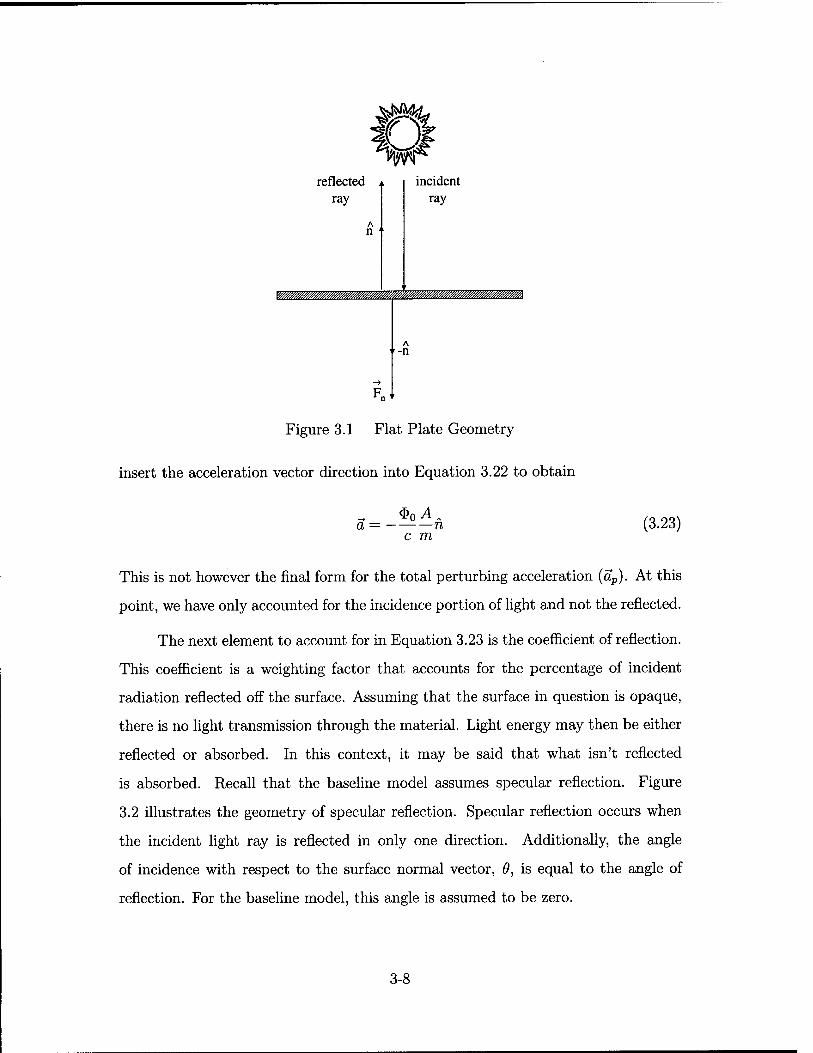
reflected ray
Ät
incident ray
F„..
Figure 3.1 Flat Plate Geometry
insert the acceleration vector direction into Equation 3.22 to obtain
a = n c m
(3.23)
This is not however the final form for the total perturbing acceleration (ap). At this
point, we have only accounted for the incidence portion of light and not the reflected.
The next element to account for in Equation 3.23 is the coefficient of reflection.
This coefficient is a weighting factor that accounts for the percentage of incident
radiation reflected off the surface. Assuming that the surface in question is opaque,
there is no light transmission through the material. Light energy may then be either
reflected or absorbed. In this context, it may be said that what isn't reflected
is absorbed. Recall that the baseline model assumes specular reflection. Figure
3.2 illustrates the geometry of specular reflection. Specular reflection occurs when
the incident light ray is reflected in only one direction. Additionally, the angle
of incidence with respect to the surface normal vector, 9, is equal to the angle of
reflection. For the baseline model, this angle is assumed to be zero.
3-8
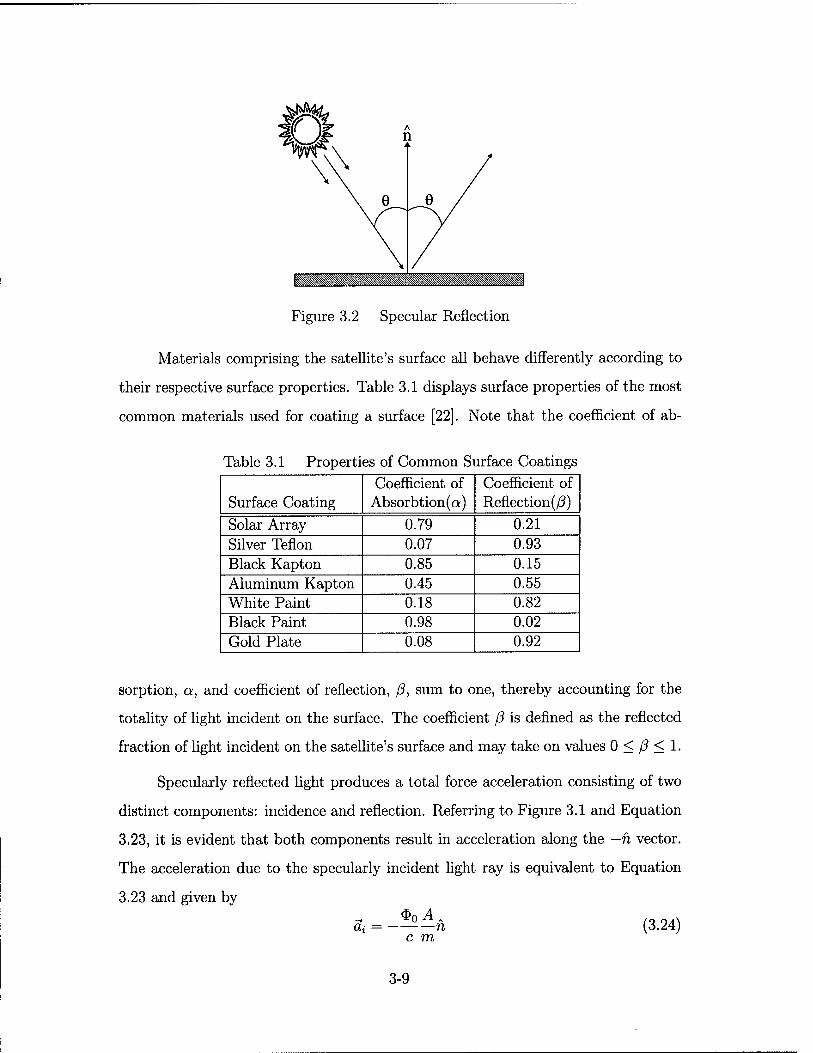
Figure 3.2 Specular Reflection
Materials comprising the satellite's surface all behave differently according to
their respective surface properties. Table 3.1 displays surface properties of the most
common materials used for coating a surface [22]. Note that the coefficient of ab-
Table 3.1 Properties of Common Surface Coatings
Surface Coating Coefficient of
Absorbtion(a;) Coefficient of Reflection(/3)
Solar Array 0.79 0.21 Silver Teflon 0.07 0.93 Black Kapton 0.85 0.15 Aluminum Kapton 0.45 0.55 White Paint 0.18 0.82 Black Paint 0.98 0.02 Gold Plate 0.08 0.92
sorption, a, and coefficient of reflection, ß, sum to one, thereby accounting for the
totality of light incident on the surface. The coefficient ß is defined as the reflected
fraction of light incident on the satellite's surface and may take on values 0 < ß < 1.
Specularly reflected light produces a total force acceleration consisting of two
distinct components: incidence and reflection. Referring to Figure 3.1 and Equation
3.23, it is evident that both components result in acceleration along the — h vector.
The acceleration due to the specularly incident light ray is equivalent to Equation
3.23 and given by
at = n (3.24) c m
3-9
The acceleration due to the specularly reflected light ray is a fraction ofthat produced
by the incident ray and is expressed as a function of ß.
Er = -ß^--h (3.25) c m
In order to obtain the total perturbing acceleration, we must now sum Equations
3.24 and 3.25. This then gives
Op = Si + a r
= n — p n cm cm
= -(1+ßfö-n (3.26) cm
Many perturbation models use Equation 3.26 as their model for SRP acceler-
ation [9, 27, 37]. To do so, they must make one additional simplifying assumption.
The implied assumption is that the solar flux constant (<&o) does not change. In
fact, the solar flux constant is only valid for the average distance from the Sun to
the Earth. This distance is defined by the semi-major axis of the Earth's orbit about
the Sun. The magnitude of solar flux thus depends on the distance from the Sun. At
an average distance from the Sun of 1 Astronomical Unit (AU), the time-rate flow
of radiant energy per unit area is called the solar flux constant. This value is given
as $o = 1367W/m2 with a variance of ±A5W/m2 by some authors [22, 27, 37], and
as $o = 1353Jy/ra2 with a variance of ±20W/m2 by others [8]. The latter value will
be adopted for the purpose of this study.
The variance in the solar flux constant given above is due to the eccentricity
of the Earth's orbit (e w 0.0167). Eccentricity results in the Earth being slightly
closer to the Sun than 1 AU for part of the year and slightly farther away for the
remainder. The SRP acceleration given in Equation 3.26 is a function of the solar
flux constant, and as such needs to be scaled accordingly to handle the variations.
SRP for the NORAD SGP4 model includes a scaling factor accounting for the time-
3-10
varying nature of solar flux, and will also be derived here for inclusion in the baseline
model (Equation 3.26).
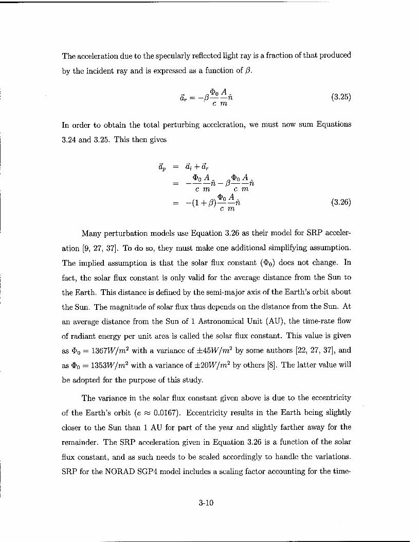
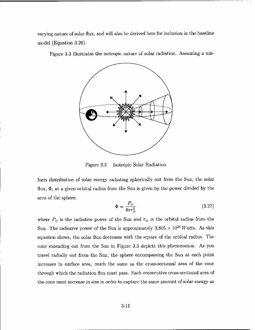
Figure 3.3 illustrates the isotropic nature of solar radiation. Assuming a uni-
4—jjyOlt ►—►—zti
yr J
Figure 3.3 Isotropic Solar Radiation
form distribution of solar energy radiating spherically out from the Sun, the solar
flux, <3>, at a given orbital radius from the Sun is given by the power divided by the
area of the sphere:
$ Pa ©
ATTTQ (3.27)
where P0 is the radiative power of the Sun and r© is the orbital radius from the
Sun. The radiative power of the Sun is approximately 3.805 x 1026 Watts. As this
equation shows, the solar flux decreases with the square of the orbital radius. The
cone extending out from the Sun in Figure 3.3 depicts this phenomenon. As you
travel radially out from the Sun, the sphere encompassing the Sun at each point
increases in surface area, much the same as the cross-sectional area of the cone
through which the radiation flux must pass. Each consecutive cross-sectional area of
the cone must increase in size in order to capture the same amount of solar energy as
3-11
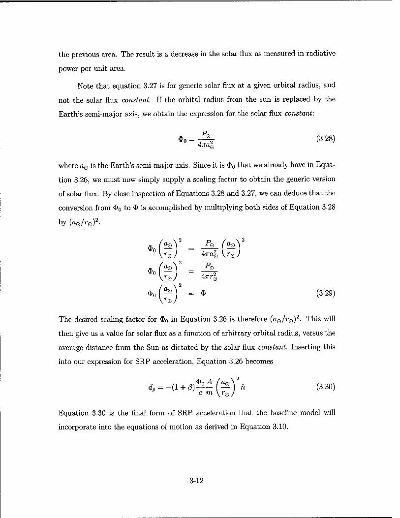
the previous area. The result is a decrease in the solar flux as measured in radiative
power per unit area.
Note that equation 3.27 is for generic solar flux at a given orbital radius, and
not the solar flux constant. If the orbital radius from the sun is replaced by the
Earth's semi-major axis, we obtain the expression for the solar flux constant:
*° = £k (3-28)
where a0 is the Earth's semi-major axis. Since it is $0 that we already have in Equa-
tion 3.26, we must now simply supply a scaling factor to obtain the generic version
of solar flux. By close inspection of Equations 3.28 and 3.27, we can deduce that the
conversion from $0 to $ is accomplished by multiplying both sides of Equation 3.28
by (a0/ro)2.
rQJ Anal \rQ
47rr£ f© J 47T7Q
$o(^) = $ (3-29)
The desired scaling factor for <&0 hi Equation 3.26 is therefore (aQ/rQ)2. This will
then give us a value for solar flux as a function of arbitrary orbital radius, versus the
average distance from the Sun as dictated by the solar flux constant. Inserting this
into our expression for SRP acceleration, Equation 3.26 becomes
ap = -(l + ß)^(^)2n (3.30) c m\rQJ
Equation 3.30 is the final form of SRP acceleration that the baseline model will
incorporate into the equations of motion as derived in Equation 3.10.
3-12
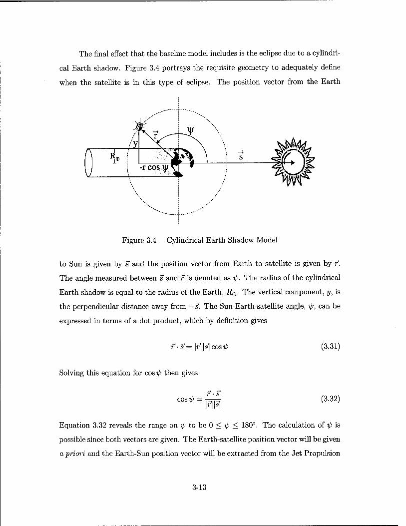
The final effect that the baseline model includes is the eclipse due to a cylindri-
cal Earth shadow. Figure 3.4 portrays the requisite geometry to adequately define
when the satellite is in this type of eclipse. The position vector from the Earth
s
Figure 3.4 Cylindrical Earth Shadow Model
to Sun is given by s and the position vector from Earth to satellite is given by f.
The angle measured between s and r is denoted as ip. The radius of the cylindrical
Earth shadow is equal to the radius of the Earth, R®. The vertical component, y, is
the perpendicular distance away from —s. The Sun-Earth-satellite angle, ip, can be
expressed in terms of a dot product, which by definition gives
r • s |r||s| cos V (3.31)
Solving this equation for cos ip then gives
cos ip r ■ s
MM (3.32)
Equation 3.32 reveals the range on ijj to be 0 < ip < 180°. The calculation of ip is
possible since both vectors are given. The Earth-satellite position vector will be given
a priori and the Earth-Sun position vector will be extracted from the Jet Propulsion
3-13
Laboratory (JPL) Planetary and Lunar Ephemerides [25]. Given the value for cos^,
we can now test whether the satellite is sunlit or in shadow. Solar illumination can
be determined by 2 cases. Case 1: The front side of the Earth facing the Sun is
determined by
If cos^ > 0, then satellite is illuminated (3.33)
This is equivalent to saying ip < 90°. Case 2: If cost/; < 0, then the satellite is
toward the backside of the Earth. When this happens, the angle between -s and f
is 180° - ip. Since cos(180° - if)) = - cos ip, the bottom side of the triangle is given
by -rcos^ as shown in Figure 3.4. Next, by Pythagorean theorem, the satellite's
position in relation to the Earth-Sun line (—s) is
r2 = y2 + (—rcos-0)2
= 2/2 + r2cos2^ (3.34)
Solving for y2 then gives
y2 = r2 - r2 cos2 ip (3.35)
Any value for y2 in Equation 3.35 greater than i?|, indicates the satellite is outside
of shadow. Case 2 then becomes
If cos ip < 0 and r2 — r2 cos2 ip > R^, then satellite is illuminated (3.36)
Obviously, if the satellite is in shadow, the SRP acceleration (ap) is zero. Armed
with Equation 3.30 and the test cases for solar illumination, Equations 3.33 and 3.36,
the baseline model for SRP acceleration is ready for inclusion in Equation 3.10.
There is one last item of notable interest before proceeding with the deriva-
tion of more complicated SRP effects. As stated earlier, the SRP model contained
in NORAD's SGP4 was assumed as the representative baseline model. The SRP
acceleration baseline model, as derived in this section in the form of Equation 3.30,
is identical to the NORAD SGP4 model with a few minor exceptions. First, while
3-14
admittedly incorrect, SGP4 assumes the SRP acceleration vector to be aligned with
the Sun-Earth vector versus the true Sun-satellite vector. Note that Equation 3.30
maintains an acceleration vector direction given by —h which is aligned with the Sun-
satellite vector. SGP4 documentation acknowledges that this assumption introduces
a small periodic error term which it states is acceptable [24].
The second minor difference lies in the use of units nomenclature. The model
previously derived in this section assumes standard System International (SI) units.
The end result is acceleration in units of m/s2. The SGP4 SRP model makes use
of both SI and canonical units. The canonical units define the SRP acceleration in
terms of Earth radii/kemin2. A kemin is a canonical time unit and is equivalent
to the time it takes a hypothetical satellite at the surface of the Earth to travel one
radian of true anomaly around the Earth. A kemin is approximately equal to 806.8
seconds. After some simplification and substitution, the units of both the SGP4
SRP model and the model derived here, can be made to agree in both form and
function. However, since SGP4 is over twenty years old, values for some of the so-
called constants; such as G, <J>0, or R$, as tabulated at that time are not the same
as today. For instance, the semi-major axis of the Earth was previously taken to be
1 AU. In reality, the value is more precisely 1.00000011 AU according to NASA's
J2000 Planetary Orbital Elements [25]. These minor differences account for very
small discrepancies in the models' constant coefficients. Otherwise, both models are
the same, and this then constitutes the baseline.
The goal now is to model improvements to the SRP model as discussed in Sec-
tion 1.4. The modeling of these effects will be realized by correspondingly modifying
the baseline embodied by Equation 3.30. A comparison of the results of these more
complex SRP effects with respect to the baseline model will determine the merit of
modeling said effects. The first, and probably most prominent of these SRP effects,
is the changing area of the satellite cross-section as perceived by the Sun.
3-15
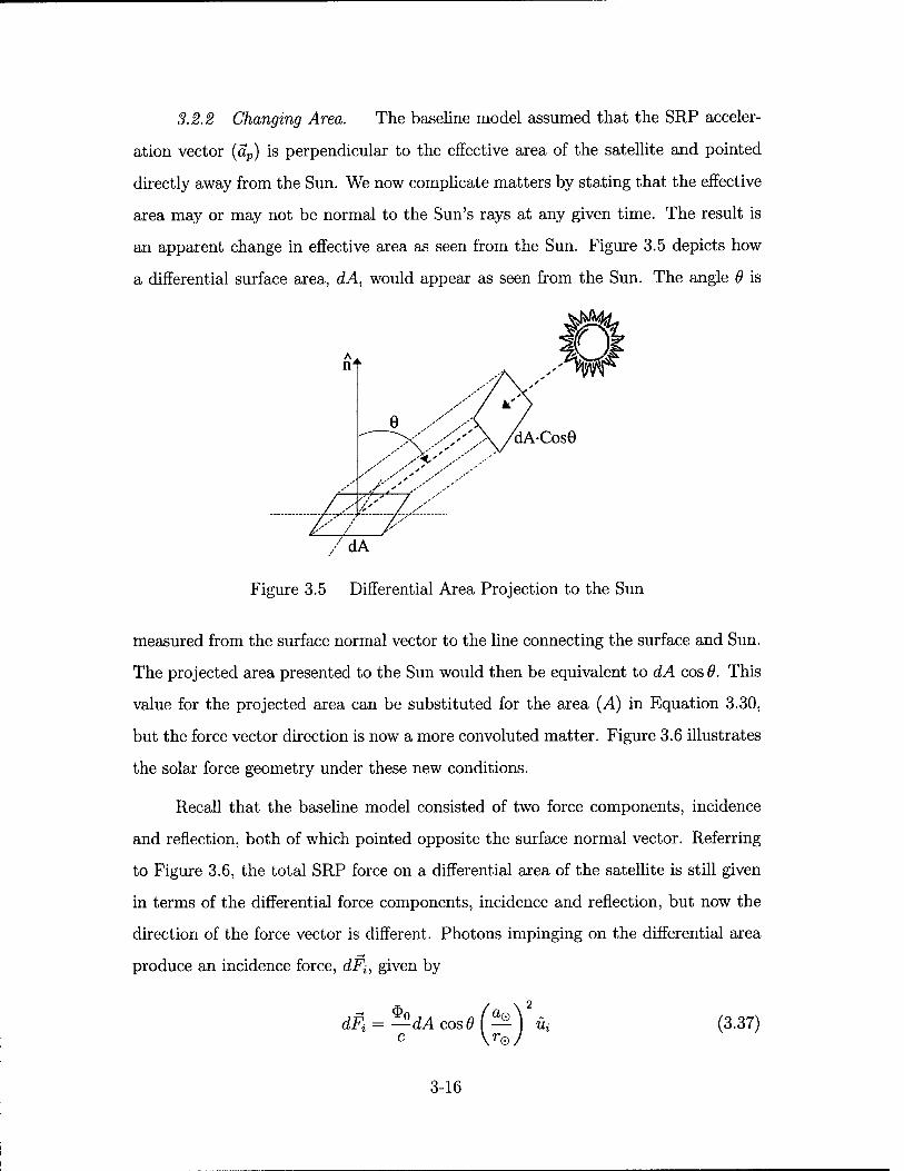
3.2.2 Changing Area. The baseline model assumed that the SRP acceler-
ation vector (äp) is perpendicular to the effective area of the satellite and pointed
directly away from the Sun. We now complicate matters by stating that the effective
area may or may not be normal to the Sun's rays at any given time. The result is
an apparent change in effective area as seen from the Sun. Figure 3.5 depicts how
a differential surface area, dA, would appear as seen from the Sun. The angle 6 is
dA-CosG
Figure 3.5 Differential Area Projection to the Sun
measured from the surface normal vector to the line connecting the surface and Sun.
The projected area presented to the Sun would then be equivalent to dA cos 6. This
value for the projected area can be substituted for the area (A) in Equation 3.30,
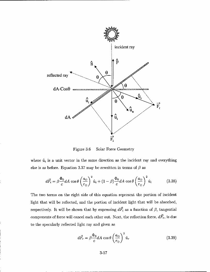
but the force vector direction is now a more convoluted matter. Figure 3.6 illustrates
the solar force geometry under these new conditions.
Recall that the baseline model consisted of two force components, incidence
and reflection, both of which pointed opposite the surface normal vector. Referring
to Figure 3.6, the total SRP force on a differential area of the satellite is still given
in terms of the differential force components, incidence and reflection, but now the
direction of the force vector is different. Photons impinging on the differential area
produce an incidence force, dFi, given by
c Vr© Ui (3.37)
3-16
incident ray
reflected ray
dA-Cos6 .
0 e
0
A Ut
\ \ V
\
0 V
k A
A \
\ r A
U- l ,-''' \ s s*
\ \ ,'
\ ,r ^ ''■
F_
F
Figure 3.6 Solar Force Geometry
where M; is a unit vector in the same direction as the incident ray and everything
else is as before. Equation 3.37 may be rewritten in terms of ß as
dPt = ß%A cosO (^Xüi + (1 - ß)%A cos9 (V * c \rQJ c \rQ
Ui (3.38)
The two terms on the right side of this equation represent the portion of incident
light that will be reflected, and the portion of incident light that will be absorbed,
respectively. It will be shown that by expressing dFi as a function of ß, tangential
components offeree will cancel each other out. Next, the reflection force, dFr, is due
to the specularly reflected light ray and given as
dFr = ß—dA cos 6 (^ ] ur c Vo.
(3.39)
3-17
where üT is a unit vector directly opposite the specularly reflected ray.
Prior to summing the constituent force components, we note that in Figure
3.6, both üi and uT can be broken into orthogonal components of the tangential unit
vector, ut, and the normal unit vector, un.
üi = cos9ün + sm.9üt (3.40)
ur = cos 9 un — sin 9 ut (3-41)
Substituting Equation 3.40 for üi in only the first term on the right side of Equation
3.38, and algebraically simplifying, the differential incidence force becomes
dFi = ß—dA cos2 9 (^] ün + ß—dAcos9sin9(^\ üt c \rQJ c \rQJ
+ (1 - ß)^dA cose (^\ üt (3.42)
Similarly, if we substitute Equation 3.41 for ür in Equation 3.39 and simplify, dFr
will be given by
dPr = ß—dA cos29 (^) ün-ß—dAcos9sm9(^) üf (3.43)
Summing Equations 3.42 and 3.43 now results in the total perturbing force acting
on a differential area of the satellite, dPp. Notice that the tangential unit vector (üt)
components cancel out and the normal unit vector (ün) components combine to give
dFp = dFi + dFr 2 ^ /_ \2
= (i-ß)*°dA<xxe(^) üi + 2ß%Acos29(^) ün (3.44) c \r0/ c \reJ
By close inspection of Figure 3.6, we observe that üi = —p, where p represents the
unit vector along the satellite-Sun line and also that ün = —n. After making these
3-18
simple vector substitutions, Equation 3.44 becomes
dpp = _(l -ß)*°dA cos0 (^)2p - 2ß%A cos2 6 (V)2n (3.45) c \r0/ c \r0/
Summarizing, Equation 3.45 gives the total SRP force on a differential area of
the satellite surface as defined thus far in this thesis. One need only divide through
by mass to obtain the SRP acceleration. The next logical step is to sum up, or rather
integrate, all the differential areas over the entire portion of the satellite's surface
currently being illuminated. This requires detailed knowledge of the satellite's shape
and surface geometry, as well as attitude. The baseline model assumed the simple
shape of a sphere or a flat plate. Section 3.2.4 will demonstrate integration of the
differential area elements over the surface of a satellite with a more complicated
shape, namely that of a cylinder. However, there is one other SRP effect that should
be considered before doing this, since it will also need to be integrated over the
surface of the satellite. The new effect is diffuse reflection.
3.2.3 Diffuse Reflection. The baseline model and Equation 3.45 both as-
sumed only specular reflection, incident light that reflects in only one direction.
Diffuse reflection is where the incident light ray reflects in many different directions.
Figure 3.7 illustrates the concept of diffuse reflection under a three dimensional hemi-
spheric bowl. The dotted lines below the hemispheric bowl represent the direction of
individual force vectors corresponding to each ray of diffusely reflected light, which
eventually will need to be summed. The goal then is to integrate over the hemisphere
to obtain the total SRP force on the differential area, dA, due to diffuse reflection.
First, it is necessary to incorporate into Equation 3.45 coefficients that account for
both specular and diffuse reflection.
Recall ß is defined to be the coefficient of reflection. Reflection can now be
either specular or diffuse. Therefore, ß is that fraction of light being reflected (both
specular and diffuse) and (l-ß) is that fraction being absorbed. Introducing a ratio
3-19
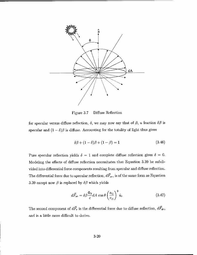
Figure 3.7 Diffuse Reflection
for specular versus diffuse reflection, 5, we may now say that of ß, a fraction Sß is
specular and (1 - S)ß is diffuse. Accounting for the totality of light thus gives
5ß+(l-8)ß + (l-ß) = l (3.46)
Pure specular reflection yields 5 = 1 and complete diffuse reflection gives S = 0.
Modeling the effects of diffuse reflection necessitates that Equation 3.39 be subdi-
vided into differential force components resulting from specular and diffuse reflection.
The differential force due to specular reflection, dFsr, is of the same form as Equation
3.39 except now ß is replaced by 6ß which yields
dFsr = 8ß—dA cos 9 a, _© r0.
Ur (3.47)
The second component of dFr is the differential force due to diffuse reflection, dFdr,
and is a little more difficult to derive.
3-20
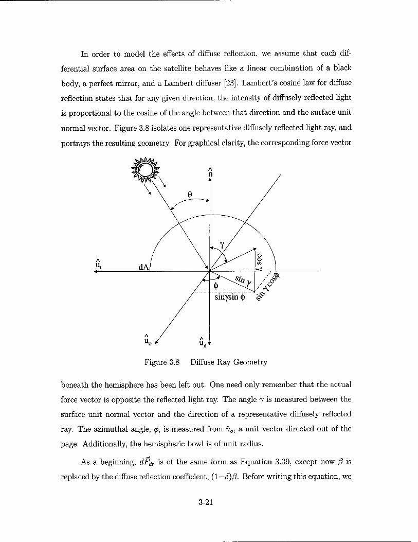
In order to model the effects of diffuse reflection, we assume that each dif-
ferential surface area on the satellite behaves like a linear combination of a black
body, a perfect mirror, and a Lambert diffuser [23]. Lambert's cosine law for diffuse
reflection states that for any given direction, the intensity of diffusely reflected light
is proportional to the cosine of the angle between that direction and the surface unit
normal vector. Figure 3.8 isolates one representative diffusely reflected light ray, and
portrays the resulting geometry. For graphical clarity, the corresponding force vector
Figure 3.8 Diffuse Ray Geometry
beneath the hemisphere has been left out. One need only remember that the actual
force vector is opposite the reflected light ray. The angle 7 is measured between the
surface unit normal vector and the direction of a representative diffusely reflected
ray. The azimuthal angle, </>, is measured from u0, a unit vector directed out of the
page. Additionally, the hemispheric bowl is of unit radius.
As a beginning, dF^r is of the same form as Equation 3.39, except now ß is
replaced by the diffuse reflection coefficient, (l-S)ß. Before writing this equation, we
3-21
note one other minor difference. Previously, the solar flux constant ($0) represented
the intensity of light, both incident on and reflected from the satellite surface. Now
because of Lambert's law, the intensity of each diffusely reflected ray of light is
proportional to cos 7 and not simply equal to $0. Therefore, scaling $0 by the factor
cos 7 produces the scalar expression
dFdr = (1 - ö)ß— cos^dA cos0 (^ J (3.48)
Equation 3.48 is not yet complete because it gives only the force contribution of
one diffusely reflected ray. Since each individual ray of diffusely scattered light will
contribute a force, they must all be summed to obtain the total differential force due
to diffusely reflected light {dFdr). It should be noted that by symmetry, all tangential
force components along both ut and u0 will cancel. This will be analytically proven
in the following analysis.
Since force is a vector, we need to assign a direction to Equation 3.48. The
unit hemispherical bowl in Figure 3.8 offers a method for defining the force vector
direction in spherical coordinates. Figure 3.8 identifies the components of the force
vector of the representative ray. Trigonometric identities, cos(7r/2 — 7) = sin 7 and
sin(7r/2 — 7) = cos 7, aid in determining these components. Recalling that the
force vector for each diffuse ray is opposite in direction to that ray, the force vector
direction is given by
sin 7 cos (fm0
sin 7 sin <^wt (3.49)
cos 7Wn
Inserting this vector direction into Equation 3.48, we now have
dFdr = (1 - S)ß— cosydA cos6 (^ c \rQ
sin 7 cos (fm0
sin 7 sin 4>ut
cos 7&n
(3.50)
3-22
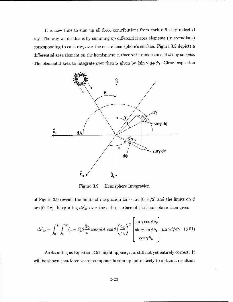
It is now time to sum up all force contributions from each diffusely reflected
ray. The way we do this is by summing up differential area elements (in steradians)
corresponding to each ray, over the entire hemisphere's surface. Figure 3.9 depicts a
differential area element on the hemisphere surface with dimensions of cfy by sin 7#.
The elemental area to integrate over then is given by (sin rfdcfid'y. Close inspection
Figure 3.9 Hemisphere Integration
of Figure 3.9 reveals the limits of integration for 7 are [0, 7r/2] and the limits on (j)
are [0, 2TT]. Integrating dF<tr over the entire surface of the hemisphere then gives
dFdr = [2 ["(1- 5)ß— cos jdA cos 9 (^ JO JO c \rQ
sin 7 cos (jm0
sin 7 sin (f)üt
cos jun
sin 'ydfid'y (3.51)
As daunting as Equation 3.51 might appear, it is still not yet entirely correct. It
will be shown that force vector components sum up quite nicely to obtain a resultant
3-23
vector in the un direction. However, this process also sums up the intensity of the
diffusely scattered light in a linear fashion, when what is required is an average
intensity. An analogy can be seen in summing up temperatures in various locations
throughout a room. The sum of these temperatures does not represent the room
temperature, but an average would. Intensity, like temperature, sums like a scalar in
this case. The obvious remedy is to divide out the totality of diffuse light to obtain
the average intensity.
Whereas the intensity in any one direction is proportional to cos 7, the total
amount of diffuse light is proportional to this value integrated over the hemisphere
as illustrated in Figure 3.9. This is represented by the integral
? /"27T
Fl Jo Jo cos 7 sin 7 d^d'y (3.52)
Therefore, if we divide Equation 3.51 by this integral, we will obtain the correct form
for total force due to diffuse reflection on a differential element of the spacecraft, dA.
JoUfil-W^ax-rdAcoBefe)2
dFdr =
sin 7 cos 4>u0
sin 7 sin (jmt
cos 7&n
sin 'ydcßd'j
Jo Jo * cos 1 s^n ld4>d-y (3.53)
This equation may now be simplified. Factoring out the constants of integration
produces
(l-ö)ß^dAcose^yj}^coS1
dFdr =
sin 7 cos 4>u0
sin 7 sin 4>ut
cos 7«n
sin 'jd^dj
So2 lo * cos 1 s^n ld(j)d^ (3.54)
3-24
There are a total of four distinct integrals that now need to be analytically evaluated.
The integrals involving u0 and ut both evaluate to zero as previously anticipated.
>S /-27T
/ / cos 7 [sin 7 cos cj)ü0] sin yd^dj = 0 (3.55) Jo Jo
/ / cos 7 [sin 7 sin (f)üt] sin 'ydcjxi'y — 0 (3.56) Jo Jo
The integral involving un evaluates to
/"f f2ir 2?r , N / / cos 7 [cos 7«n] sin 7d0d7 = — un (3.57)
Finally, the integral in the denominator accounting for the totality of diffuse light,
evaluates as
/ / cos 7 sin 'ydfid'j = TT (3.58) Jo Jo
Substituting each of the four integral evaluations into Equation 3.54, we can further
simplify to obtain
(1 -5)ß**dA cos0 fe)2fün dFdr = ^ V°; (3.59)
Rearranging variables and canceling the n terms gives the final and most desirable
form of dFdr-
dFdr = (l-5)ß~dAcoso(^\ ün (3.60)
The total perturbing force on a differential area of the satellite's surface due
to SRP can now be expressed as a sum of the constituent components. The three
differential force components include incidence (GLFJ) from Equation 3.38, specular
reflection (dFsr) from Equation 3.47, and diffuse reflection (dFdr) from Equation
3.60.
dF = dPi + dPsr + dPdr (3.61)
Directly substituting the expressions for these components as previously derived,
and algebraically subdividing the first term of dPi and expressing as a function of S,
3-25
results in
dF = 6ß%A cos9 (^Xü, + {l-S)ß^dAcoß0(^\\
+ (i _ ß)*±dA cos 9 (^\ in + Sß^dA cos9 (^\ ur
+ (1 - 5)ß\^dA cos9 (^)\ (3-62) 3 c \r0/
The terms comprising Equation 3.62 denote in order: the incidence force due to
the fraction of light that will be specularly reflected, the incidence force due to the
fraction of light that will be diffusely reflected, the incidence force due to the fraction
of light that will be absorbed, the force due to specular reflection, and the force due
to diffuse reflection.
As seen before in Section 3.2.2, tangential components of force may be made
to drop out by transforming üi and ur in the first and fourth terms of Equation 3.62,
into components of un and ut. Following some algebraic simplification and making
the same unit vector substitutions as before, üi = —p and un = —n, the total SRP
force on a differential area of the satellite's surface becomes
dF = 2Sß—dA cos2 9 + (1 - 6)ß^—dA cos 9 c o c
2
^) h (3.63)
-(l-5ß)%Acos9(a^)2p c Vro/
As stated earlier, one need only divide through by mass to obtain the desired per-
turbing SRP acceleration (ap) that will be included in the equations of motion of
Equation 3.10. Equation 3.63 now needs to be integrated over the entire portion
of the satellite's surface currently being illuminated, thereby summing the force
contributions of each differential area, and arriving at the total perturbing SRP ac-
celeration on the satellite. This requires insight into the satellite's attitude and basic
shape.
3-26
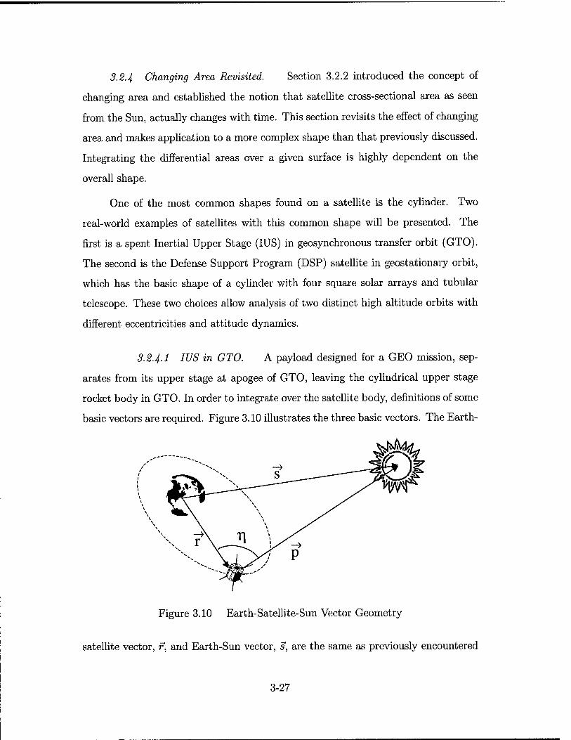
3.2.4 Changing Area Revisited. Section 3.2.2 introduced the concept of
changing area and established the notion that satellite cross-sectional area as seen
from the Sun, actually changes with time. This section revisits the effect of changing
area and makes application to a more complex shape than that previously discussed.
Integrating the differential areas over a given surface is highly dependent on the
overall shape.
One of the most common shapes found on a satellite is the cylinder. Two
real-world examples of satellites with this common shape will be presented. The
first is a spent Inertial Upper Stage (IUS) in geosynchronous transfer orbit (GTO).
The second is the Defense Support Program (DSP) satellite in geostationary orbit,
which has the basic shape of a cylinder with four square solar arrays and tubular
telescope. These two choices allow analysis of two distinct high altitude orbits with
different eccentricities and attitude dynamics.
3.2.4.I IUS in GTO. A payload designed for a GEO mission, sep-
arates from its upper stage at apogee of GTO, leaving the cylindrical upper stage
rocket body in GTO. In order to integrate over the satellite body, definitions of some
basic vectors are required. Figure 3.10 illustrates the three basic vectors. The Earth-
Figure 3.10 Earth-Satellite-Sun Vector Geometry
satellite vector, f, and Earth-Sun vector, s, are the same as previously encountered
3-27
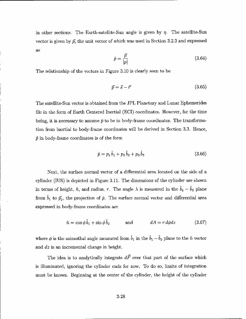
in other sections. The Earth-satellite-Sun angle is given by 77. The satellite-Sun
vector is given by p, the unit vector of which was used in Section 3.2.3 and expressed
as
P = n (3-64) bl The relationship of the vectors in Figure 3.10 is clearly seen to be
p = s-f (3.65)
The satellite-Sun vector is obtained from the JPL Planetary and Lunar Ephemerides
file in the form of Earth Centered Inertial (ECI) coordinates. However, for the time
being, it is necessary to assume p to be in body-frame coordinates. The transforma-
tion from inertial to body-frame coordinates will be derived in Section 3.3. Hence,
p in body-frame coordinates is of the form
p = Pibi+p2b2+ Pz h (3.66)
Next, the surface normal vector of a differential area located on the side of a
cylinder (IUS) is depicted in Figure 3.11. The dimensions of the cylinder are shown
in terms of height, h, and radius, r. The angle A is measured in the bi — b2 plane
from bi to pj, the projection of p. The surface normal vector and differential area
expressed in body-frame coordinates are
ft = cos (j) b\ + sin <f> b2 and dA = r d(j)dz (3.67)
where 4> is the azimuthal angle measured from b\ in the &i — b2 plane to the n vector
and dz is an incremental change in height.
The idea is to analytically integrate dF over that part of the surface which
is illuminated, ignoring the cylinder ends for now. To do so, limits of integration
must be known. Beginning at the center of the cylinder, the height of the cylinder
3-28
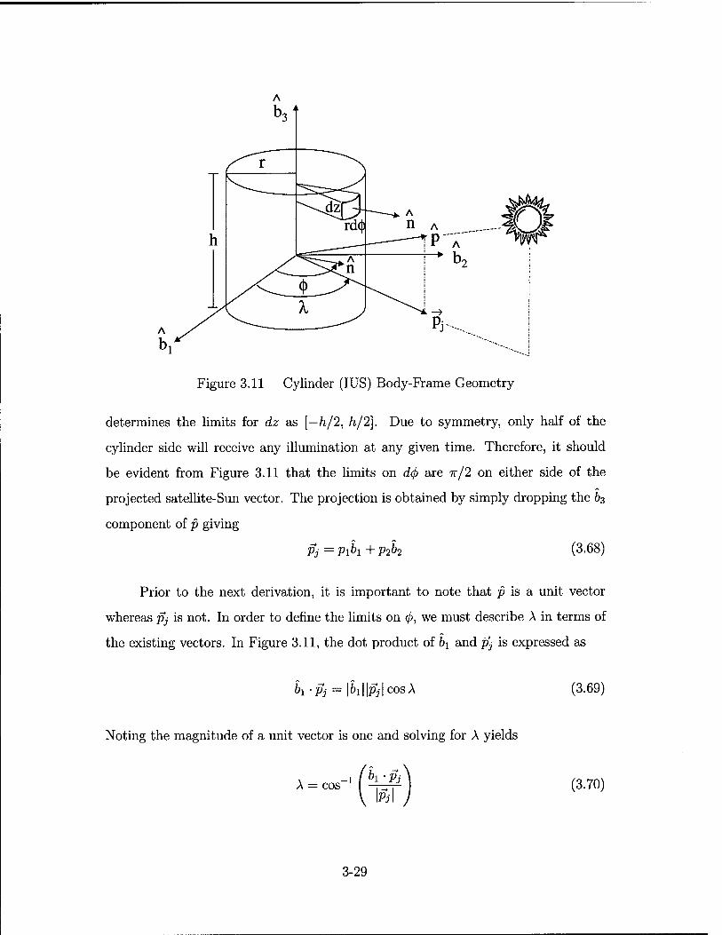
Figure 3.11 Cylinder (IUS) Body-Frame Geometry
determines the limits for dz as [—h/2, h/2]. Due to symmetry, only half of the
cylinder side will receive any illumination at any given time. Therefore, it should
be evident from Figure 3.11 that the limits on dcß are n/2 on either side of the
projected satellite-Sun vector. The projection is obtained by simply dropping the b3
component of p giving
Pj=Pibi+P2h (3-68)
Prior to the next derivation, it is important to note that p is a unit vector
whereas Pj is not. In order to define the limits on </>, we must describe A in terms of
the existing vectors. In Figure 3.11, the dot product of bi and Pj is expressed as
bi-Pj = \h\\Pj\ cosX (3.69)
Noting the magnitude of a unit vector is one and solving for A yields
A = cos" -l / kl • Pi
\Pj\ (3.70)
3-29
A quadrant ambiguity exists when A > 180°. The appropriate quadrant correction
is performed by checking if Pj -b2<0, then A = 2n - A. Having sufficiently defined
A, the limits of integration on d<j> are then expressed as [A - 7r/2, A + w/2].
Integrating over the sunlit side of the cylinder by applying the limits of integra-
tion to dF of Equation 3.63, and substituting for dA from Equation 3.67 produces
the following expression for the total SRP force applied to the cylinder's side.
/, side - CI. 2Sß— cos2 6 + (1 - 6)ß%— cos 6 C o C
-(l-5ß)~-cose(^) p)rd(j>dz
:s: n
(3.71)
We are not including the cylinder ends in this iteration of integration. The double
integral in Equation 3.71 can immediately be collapsed to a single integral since there
is no term in the integrand involving the height (h). The result is an additional factor
of h. Evaluating the inner integral and rearranging or factoring out some common
terms thus transforms Equation 3.71 to
/ side - £>( 2Sß— cos2 6 + (1 - S)ßl— cos0 c o c
n
- (l-Sß)—cos6p \d(j) (3.72)
Equation 3.72 presents an integral that must be evaluated with respect to (j),
but the integrand is in terms of 6. To continue, we must therefore find a way to
describe 6 in terms of <j>. Recall that 9 is denned as the angle measured between the
surface normal vector (n) and the satellite-Sun vector (p) as depicted in Figure 3.6,
but omitted in Figure 3.11 for graphical clarity. By definition of the dot product,
and unit vectors having magnitude of one, these two vectors surrender the needed
relationship.
cos $ = h-p (3.73)
3-30
Substituting the component form of both vectors from Equations 3.66 and 3.67 into
Equation 3.73 gives
cos 6 = (cos <f> bi + sin (j> b2) ■ (pih + p2b2 + P3h)
= pi cos (f) + P2 sin (j) (3.74)
It is now possible to replace cos 6 in Equation 3.72 with the newly derived expression
from Equation 3.74, thereby resulting in
/1 A-5 rHS, 2^5» (;
c \ Px cos 0 + p2 sin 0 ] (3.75)
+ {\-§)ß- — (picos0 + p2sin(/>j 3 c
$0
n
(1 -8ß) — (pi cos(ß + p2 sin<j))p > d(f)
We now substitute body-frame coordinates for n from Equation 3.67 and for p from
Equation 3.66 to obtain
fside = T?r/i(^) I" 2^(plCos^ + p2sin0)2 (3.76)
+ (1 - S)ß-— (piCos</> + p2sm0j ( cos 0 61 + sin0&2J
$0 - (1 - Sß)—(pi cos0 + p2 sin0j fpx 61 + p2 b2 + P3 h) f d<j>
The integrand of Equation 3.76 is now given in terms of 0, allowing us to
evaluate the integral with respect to <j>. The next step is to algebraically simplify
and combine like terms into groups of body-frame elements in hi, b2, and 63. Doing
this results in an expression consisting of three integrals, one for each body-frame
3-31
element.
hide = / rh ( — ) — - 2<5/?p2 cos3 <j) - 46ßp!p2 cos2 0 sin <f> (3.77)
2 2 -28ßp\ sin2 </> cos 0 - (1 - S)ß-pi cos2 0 - (1 - 8)ß-p2 sin 0 cos 0
-(1 - <5/?)p2 cos (p - (1 - Sß)p1p2 sin 0 &i d0
A * vr©y c 2<5/3pf cos 0 sin 0 - ASßpip2 cos 0 sin 0
2 2 -2^/?p2 sin3 <f>- (1- S)ß-pi sin 0 cos 0 - (1 - S)ß-p2 sin2 0
-(1 — öß)pip2 cos 0 — (1 — <5/?)p2 sin (/> b2d(j)
+ A-? Vr©
$0
c (1 - 6ß)pip3 cos 0 - (1 - Sß)p2p3 sin ^ 63d^>
Integrating Equation 3.77 one term at a time, and keeping the body-frame elements
together, the SRP force on the side of the cylinder becomes
/, side -5ßp\ cos A (sin2 A + 2) - -Sßp1p2 sin3 A - -5ßp\ cos3 A
+ q/?Pi7r (<*-!) + 2p2 cos A (5/? - 1) + 2Plp2 sin A ((5/3 - 1) 6i
+ -5ßp\ sin3 A - -8ßpip2 cos3 A - -<J/3pa sin A (cos2 A + 2) do O
+ ^P27r (6 - 1) + 2pip2 cos A (<5/3 - 1) + 2p2 sin A (5/? - 1)
+ 2p3 (<5/3-l) (pi cos A + p2 sin A) 63 }rh r0y c
(3.78)
Equation 3.78 is of the form that will be included in the equations of motion to be
numerically integrated after the vector is transformed to the inertial frame. How-
3-32
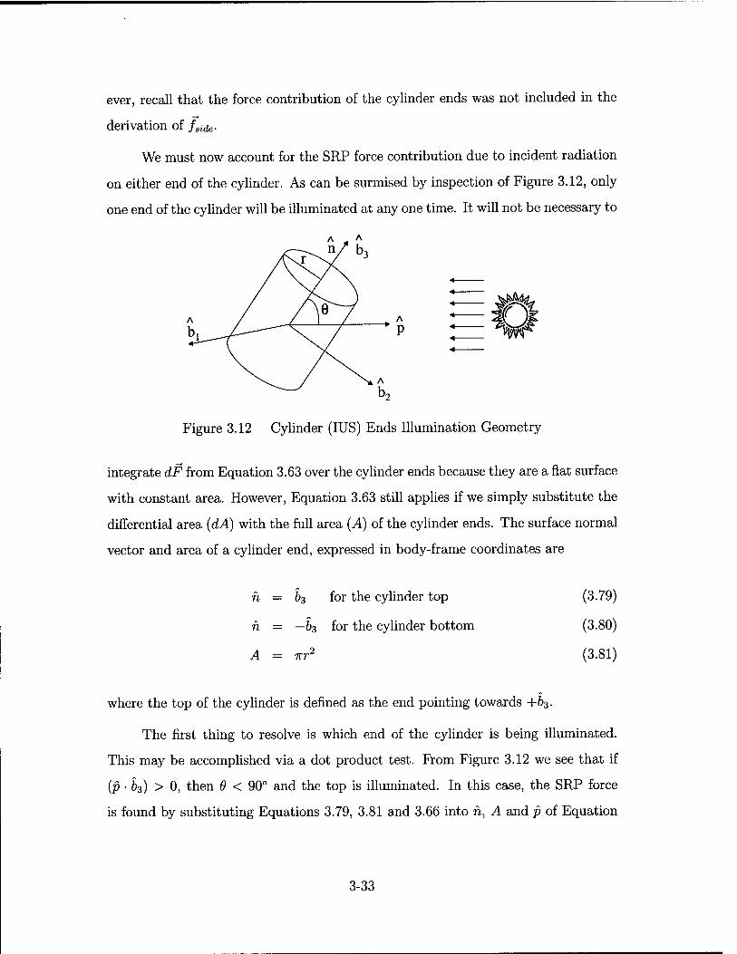
ever, recall that the force contribution of the cylinder ends was not included in the —*
derivation of faide.
We must now account for the SRP force contribution due to incident radiation
on either end of the cylinder. As can be surmised by inspection of Figure 3.12, only
one end of the cylinder will be illuminated at any one time. It will not be necessary to
A „ A b, n
/r/ A / - n ! bi^A^ P J
A
b2
Figure 3.12 Cylinder (IUS) Ends Illumination Geometry
integrate dF from Equation 3.63 over the cylinder ends because they are a flat surface
with constant area. However, Equation 3.63 still applies if we simply substitute the
differential area (dA) with the full area (A) of the cylinder ends. The surface normal
vector and area of a cylinder end, expressed in body-frame coordinates are
n = &3 for the cylinder top
n = — 83 for the cylinder bottom
irr
(3.79)
(3.80)
(3.81)
where the top of the cylinder is defined as the end pointing towards +b3.
The first thing to resolve is which end of the cylinder is being illuminated.
This may be accomplished via a dot product test. From Figure 3.12 we see that if
(p ■ h) > 0, then 9 < 90° and the top is illuminated. In this case, the SRP force
is found by substituting Equations 3.79, 3.81 and 3.66 into h, A and p of Equation
3-33
3.63, being careful to remember that dA is replaced by A.
Jtop = 25/?—Trr2 cos2 9 + (1 - S)ß\ — nr2 cos 0 a0
71 7" UUS (7 I 3 c J Vr0
-(1 - Sß)^nr2 cos9 f ^) (Plh + p2b2 + p3b3) c \re/
(3.82)
It is necessary at this point to express 9 in terms of known variables. Equation 3.73
states cos 9 as a dot product of n and p. With both of these vectors being previously
defined in Equations 3.79 and 3.66, respectively, cos# becomes
cos9 = b3- (pib1+p2b2+p3b3)
= Pz (3.83)
After some algebraic simplification and factoring out of like terms, as well as replacing
cos# with p3, Equation 3.82 becomes
ftop = ^ VW ^ (Sß-l)pi bi + (Sß-l)P2 (3.84)
+ (Sß-1)p3-26ßp3--(l-6)ß
A similar derivation follows for the bottom of the cylinder. If (p • b3) < 0, then
9 > 90° and the bottom is illuminated. Following the same substitution process as
for the cylinder top, and recalling that now n = —b3, the SRP force on the bottom
of the cylinder is expressed as
- 2 /o©\ $o A* = nr ^-j -P3< (öß-l)Pi bi + (Sß - 1)P2 (3.85)
+ (Sß-l)p3 + 2Sßp3 + -(l-6)ß
3-34
Note the only difference between ftop of Equation 3.84 and fbot of Equation 3.85
is a sign change in two terms. One test remains concerning the cylinder ends. If
(p-b3) = 0, then 8 = 90° and neither end is illuminated. In this case, both equations
would evaluate to zero since there is no 63 component of p.
In summary for an IUS in GTO, if the total SRP force acting on a cylinder is
given by fws, then as a function of Equation 3.78 and either Equation 3.84 or 3.85,
we obtain
flUS = fsides + fend (3.86)
where
fend = flap ^ {P ' h) > 0 Or
fend = fbot if (P • 63) < 0
Once Equation 3.86 is divided through by mass and transformed to the inertial
frame to obtain the perturbing acceleration (ap), it can be included in the equations
of motion of Equation 3.10, and is then ready to be numerically integrated via
computer simulation.
3.2.4.2 DSP in GEO. The previous derivation is sufficient in de-
scribing the SRP force on a simplified model of an IUS in GTO. The second satellite
to be modeled is the DSP in a geostationary orbit. Information concerning DSP in
this thesis is available in open source and is in no way classified. Some numerical
values on dimensions have been fabricated for simulation purposes. Sample orbital
elements and physical dimensions of both the DSP and IUS cases used in the simula-
tion of SRP, can be found in Section 4.1. The body geometry of DSP is illustrated in
Figure 3.13. The four solar panels are assumed to be canted downward 45° from the
b\ — b2 plane. Solar panel number 4 is in the back of Figure 3.13 and is therefore not
shown. The spin-rate of DSP about 63 is given by Q in revolutions per minute (rpm).
The telescope assembly mounted on one end of the cylinder is neglected in the SRP
3-35
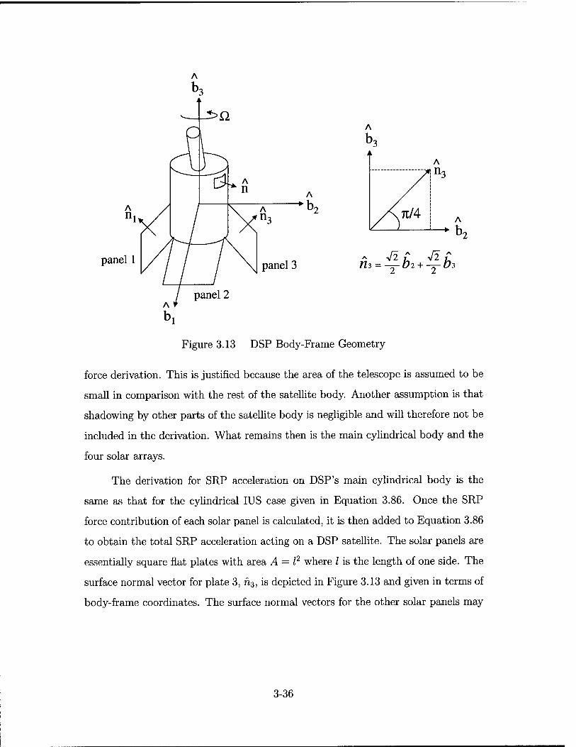
panel 1 panel 3 h^ = ^-k + ^-k
Figure 3.13 DSP Body-Frame Geometry
force derivation. This is justified because the area of the telescope is assumed to be
small in comparison with the rest of the satellite body. Another assumption is that
shadowing by other parts of the satellite body is negligible and will therefore not be
included in the derivation. What remains then is the main cylindrical body and the
four solar arrays.
The derivation for SRP acceleration on DSP's main cylindrical body is the
same as that for the cylindrical IUS case given in Equation 3.86. Once the SRP
force contribution of each solar panel is calculated, it is then added to Equation 3.86
to obtain the total SRP acceleration acting on a DSP satellite. The solar panels are
essentially square flat plates with area A = I2 where I is the length of one side. The
surface normal vector for plate 3, n3, is depicted in Figure 3.13 and given in terms of
body-frame coordinates. The surface normal vectors for the other solar panels may
3-36
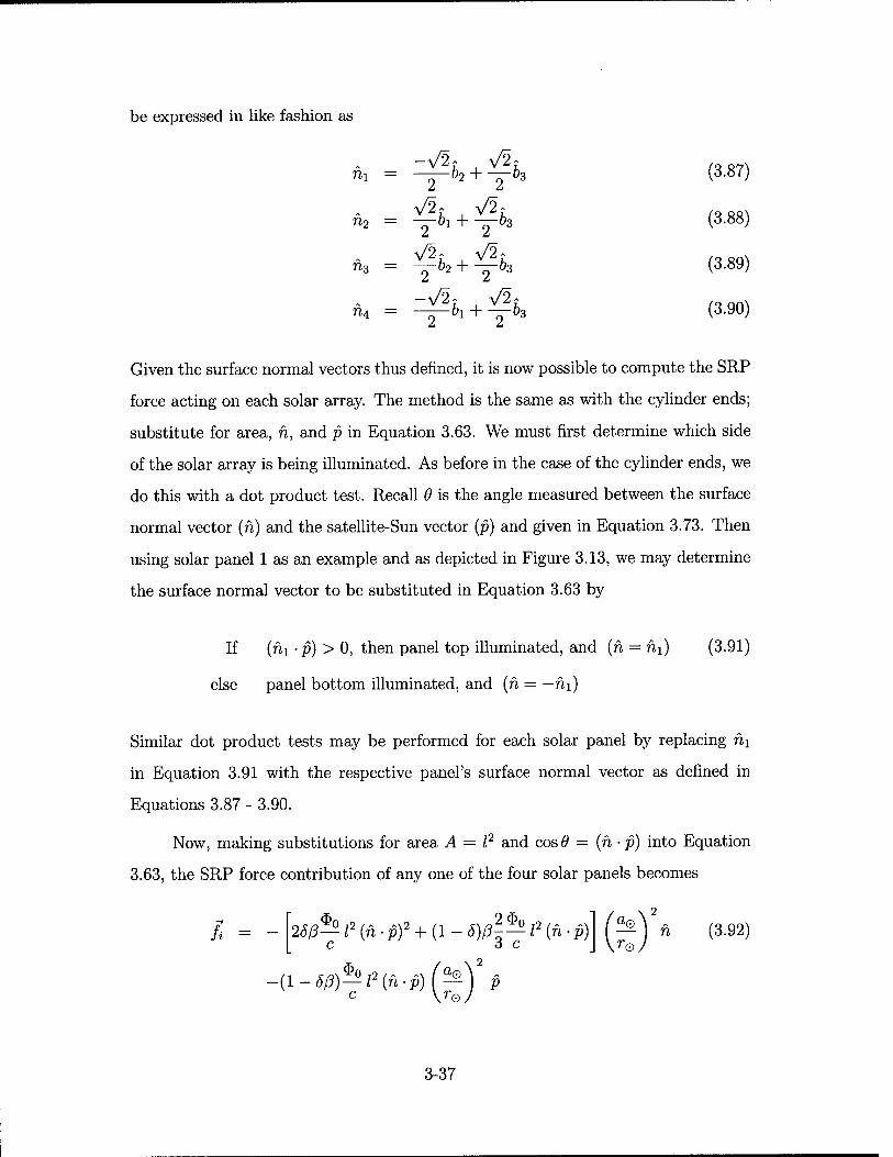
be expressed in like fashion as
ni
n4
-A j- A
A ^ A
-^ + — fts
~61 + l"**
(3.87)
(3.88)
(3.89)
(3.90)
Given the surface normal vectors thus defined, it is now possible to compute the SRP
force acting on each solar array. The method is the same as with the cylinder ends;
substitute for area, h, and p in Equation 3.63. We must first determine which side
of the solar array is being illuminated. As before in the case of the cylinder ends, we
do this with a dot product test. Recall 9 is the angle measured between the surface
normal vector (n) and the satellite-Sun vector (p) and given in Equation 3.73. Then
using solar panel 1 as an example and as depicted in Figure 3.13, we may determine
the surface normal vector to be substituted in Equation 3.63 by
If (hi -p) > 0, then panel top illuminated, and (n = hi) (3.91)
else panel bottom illuminated, and (n = — hi)
Similar dot product tests may be performed for each solar panel by replacing hi
in Equation 3.91 with the respective panel's surface normal vector as defined in
Equations 3.87 - 3.90.
Now, making substitutions for area A = I2 and cos 6 = (h • p) into Equation
3.63, the SRP force contribution of any one of the four solar panels becomes
fi = 2Sß^ I2 (h ■ pf + (1 - 5)ß\^ I2 (h • p) c 3 c
-(l-6ß)^l2(h.p) (I)'*
a, _© n (3.92)
3-37
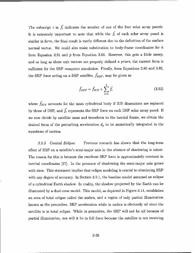
The subscript i in fa indicates the number of one of the four solar array panels.
It is extremely important to note that while the /* of each solar array panel is
similar in form, the final result is vastly different due to the definition of the surface
normal vector. We could also make substitution to body-frame coordinates for h
from Equation 3.91 and p from Equation 3.66. However, this gets a little messy,
and as long as these unit vectors are properly defined a priori, the current form is
sufficient for the SRP computer simulation. Finally, from Equations 3.86 and 3.92,
the SRP force acting on a DSP satellite, JDSP, may be given as
4
fDSP = fws + J2fi <3-93) t=l
where fIUS accounts for the main cylindrical body if IUS dimensions are replaced
by those of DSP, and f{ represents the SRP force on each DSP solar array panel. If
we now divide by satellite mass and transform to the inertial frame, we obtain the
desired form of the perturbing acceleration ap to be numerically integrated in the
equations of motion.
3.2.5 Conical Eclipse. Previous research has shown that the long-term
effect of SRP on a satellite's semi-major axis in the absence of shadowing is minor.
The reason for this is because the resultant SRP force is approximately constant in
inertial coordinates [27]. In the presence of shadowing the semi-major axis grows
with time. This statement implies that eclipse modeling is crucial to simulating SRP
with any degree of accuracy. In Section 3.2.1, the baseline model assumed an eclipse
of a cylindrical Earth shadow. In reality, the shadow projected by the Earth can be
illustrated by a dual-cone model. This model, as depicted in Figure 3.14, establishes
an area of total eclipse called the umbra, and a region of only partial illumination
known as the penumbra. SRP acceleration while in umbra is obviously nil since the
satellite is in total eclipse. While in penumbra, the SRP will not be nil because of
partial illumination, nor will it be in full force because the satellite is not receiving
3-38
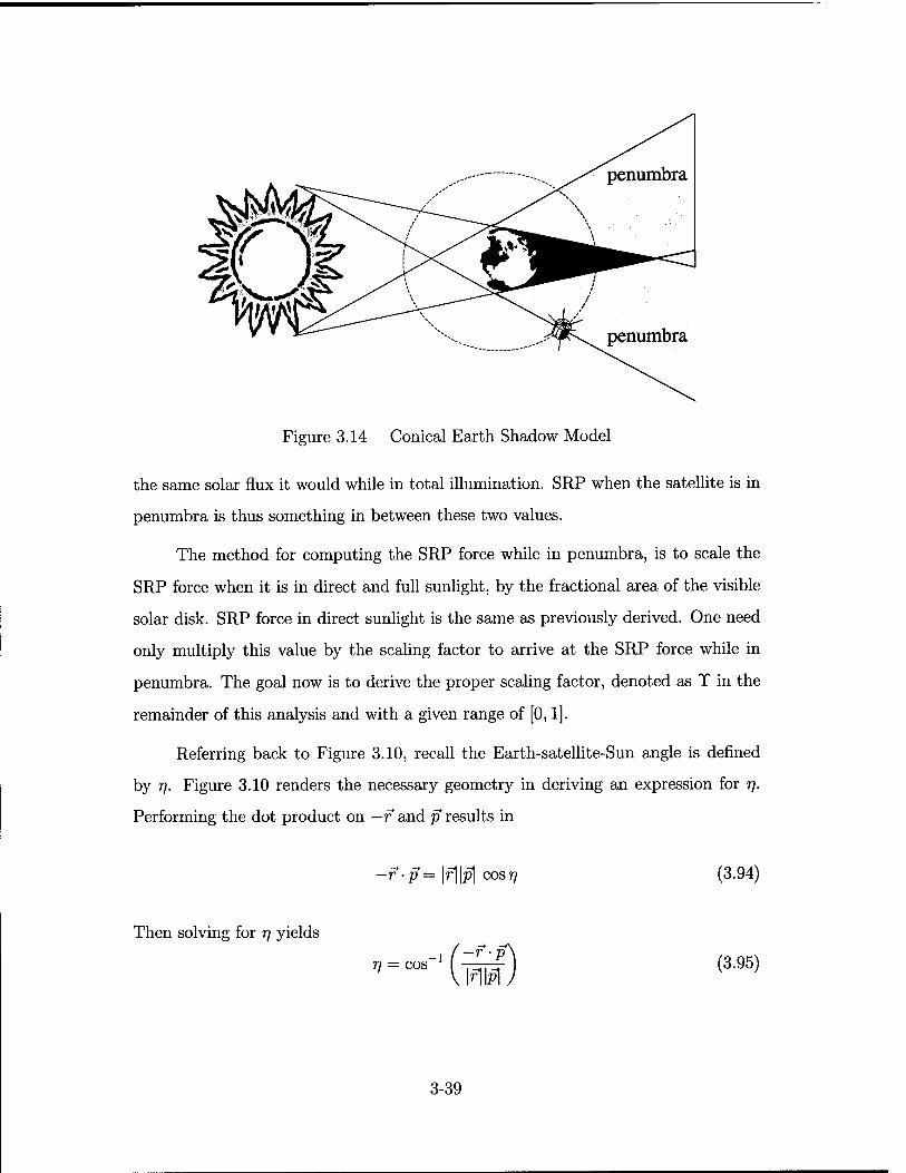
Figure 3.14 Conical Earth Shadow Model
the same solar flux it would while in total illumination. SRP when the satellite is in
penumbra is thus something in between these two values.
The method for computing the SRP force while in penumbra, is to scale the
SRP force when it is in direct and full sunlight, by the fractional area of the visible
solar disk. SRP force in direct sunlight is the same as previously derived. One need
only multiply this value by the scaling factor to arrive at the SRP force while in
penumbra. The goal now is to derive the proper scaling factor, denoted as T in the
remainder of this analysis and with a given range of [0,1].
Referring back to Figure 3.10, recall the Earth-satellite-Sun angle is defined
by rj. Figure 3.10 renders the necessary geometry in deriving an expression for rj.
Performing the dot product on — r and p results in
—f'p= \r\\p\ cos77 (3.94)
Then solving for rj yields
rj = cos —r ■ p
(3.95)
3-39
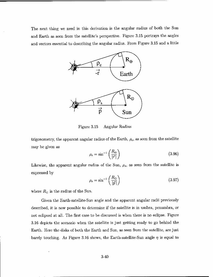
The next thing we need in this derivation is the angular radius of both the Sun
and Earth as seen from the satellite's perspective. Figure 3.15 portrays the angles
and vectors essential to describing the angular radius. From Figure 3.15 and a little
Figure 3.15 Angular Radius
trigonometry, the apparent angular radius of the Earth, pe, as seen from the satellite
may be given as
Pe = sin"1 (^ (3.96)
Likewise, the apparent angular radius of the Sun, ps, as seen from the satellite is
expressed by
ps = sin" AP\
(3.97)
where RQ is the radius of the Sun.
Given the Earth-satellite-Sun angle and the apparent angular radii previously
described, it is now possible to determine if the satellite is in umbra, penumbra, or
not eclipsed at all. The first case to be discussed is when there is no eclipse. Figure
3.16 depicts the scenario when the satellite is just getting ready to go behind the
Earth. Here the disks of both the Earth and Sun, as seen from the satellite, are just
barely touching. As Figure 3.16 shows, the Earth-satellite-Sun angle r\ is equal to
3-40
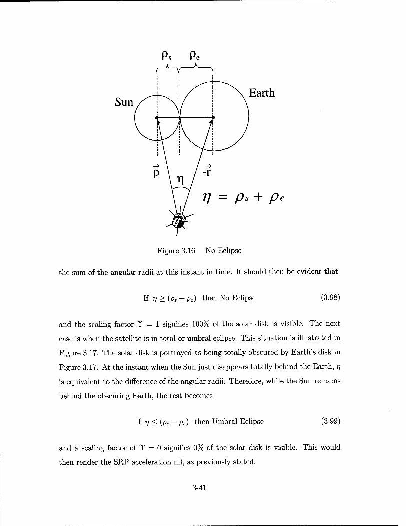
Sun Earth
7] = ps + p<
Figure 3.16 No Eclipse
the sum of the angular radii at this instant in time. It should then be evident that
If 77 > (ps + pe) then No Eclipse (3.98)
and the scaling factor T = 1 signifies 100% of the solar disk is visible. The next
case is when the satellite is in total or umbral eclipse. This situation is illustrated in
Figure 3.17. The solar disk is portrayed as being totally obscured by Earth's disk in
Figure 3.17. At the instant when the Sun just disappears totally behind the Earth, 77
is equivalent to the difference of the angular radii. Therefore, while the Sun remains
behind the obscuring Earth, the test becomes
If 77 < (pe — ps) then Umbral Eclipse (3.99)
and a scaling factor of T = 0 signifies 0% of the solar disk is visible. This would
then render the SRP acceleration nil, as previously stated.
3-41
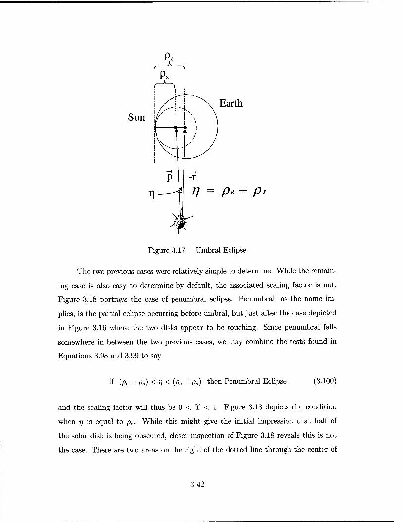
Sun Earth
= P*- P
Figure 3.17 Umbral Eclipse
The two previous cases were relatively simple to determine. While the remain-
ing case is also easy to determine by default, the associated scaling factor is not.
Figure 3.18 portrays the case of penumbral eclipse. Penumbral, as the name im-
plies, is the partial eclipse occurring before umbral, but just after the case depicted
in Figure 3.16 where the two disks appear to be touching. Since penumbral falls
somewhere in between the two previous cases, we may combine the tests found in
Equations 3.98 and 3.99 to say
If (pe — ps) < T) < (pe + Ps) then Penumbral Eclipse (3.100)
and the scaling factor will thus be 0 < T < 1. Figure 3.18 depicts the condition
when r] is equal to pe. While this might give the initial impression that half of
the solar disk is being obscured, closer inspection of Figure 3.18 reveals this is not
the case. There are two areas on the right of the dotted line through the center of
3-42
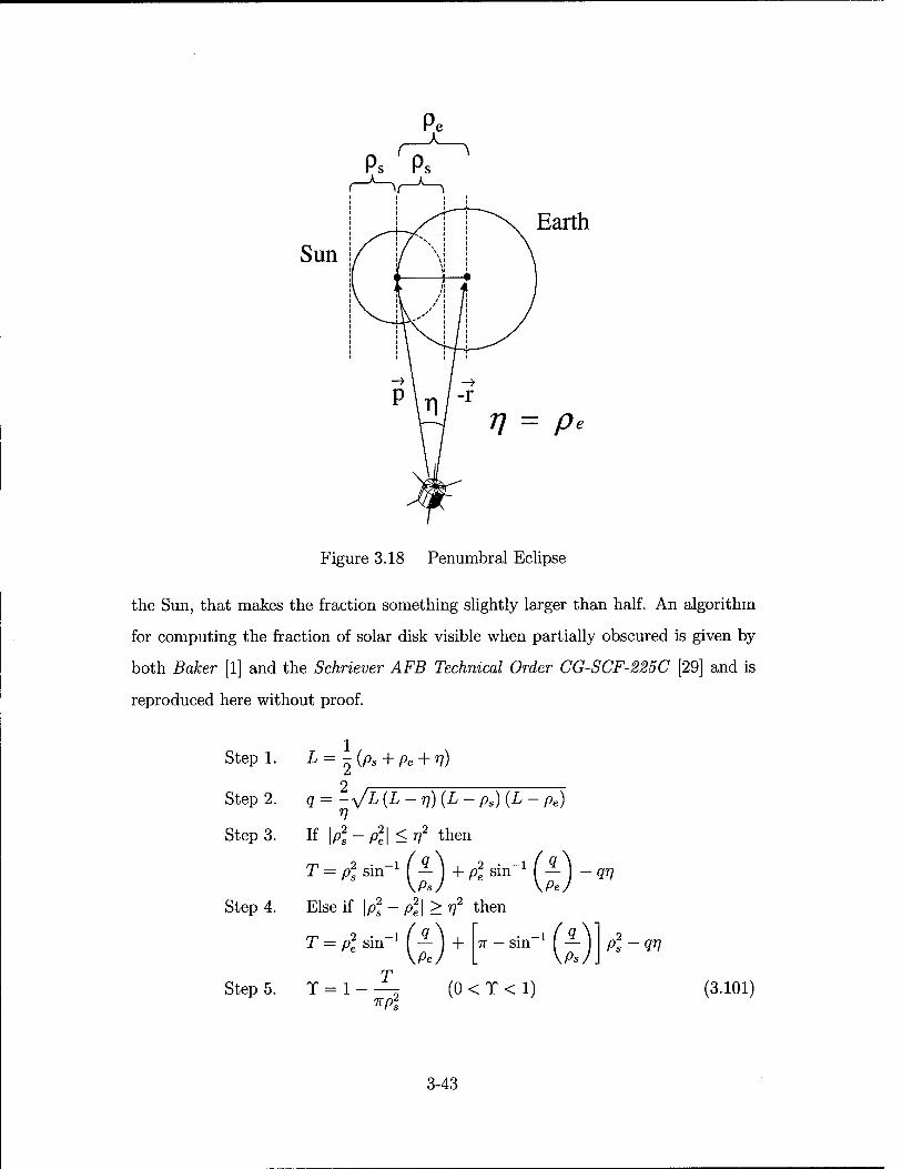
Sun Earth
n = p>
Figure 3.18 Penumbral Eclipse
the Sun, that makes the fraction something slightly larger than half. An algorithm
for computing the fraction of solar disk visible when partially obscured is given by
both Baker [1] and the Schriever AFB Technical Order CG-SCF-225C [29] and is
reproduced here without proof.
1 Step 1. L=7,(Ps + Pe + V)
o Step 2. q = -yjL(L-r))(L- ps) (L - pe)
Step 3. If \pl-pl\<rf then T=^in-'(£)+^-(£H,
Step 4. Else if \p2s - Pel > r]2 then
T-**°-l(ä+ 7T — sm — \PsJ.
P2s
Step 5. T = 1 - -^ (0 < T < 1) Kpi
qr\
(3.101)
3-43
Finally, the previously derived SRP acceleration is now multiplied by the scaling
factor (T) to obtain the most correct value for SRP acceleration due to eclipsing
effects.
The conical eclipse model just derived assumed the angular radius of the Sun
(ps), as seen from the satellite, is smaller than the angular radius of the Earth (pe).
The point at which the angular radius of the Earth becomes as small as the Sun,
may be ascertained by setting Equation 3.96 equal to Equation 3.97 as depicted in
Figure 3.15. This condition yields
§ = fe (3-102) \P\ \r\
We therefore seek the value of r from Equation 3.102. The greatest value of \p\ is
during eclipse when the satellite is directly opposite the Sun. The value of \p\ in this
case is approximately 1AU + r. Substituting this and approximate values for the
constants gives 695508 km 6378 km
1.5 x 10⁸ km + r r
Now solving for r gives a value of r « 1.4 x 10⁶ km, which means a satellite would
have to be a little less then 1.5 million km away from Earth before the angular radii
are equivalent. Hence, we are justified in saying ps < pe for any orbiting satellite in
the near-Earth environment.
3.3 Coordinate Transformations
The satellite-Sun vector (p) was first introduced in Section 3.2.4 and assumed
to be in body-frame coordinates. In actuality, p is given in the ECI frame and must be
transformed to the body frame prior to being used in any of the previous SRP force
derivation. Additionally, differences in assumed satellite attitude dynamics exist
between the IUS and DSP examples that require separate and distinct transformation
matrices. The transformation from inertial to body-frame coordinates for the IUS
will be presented first.
3-44
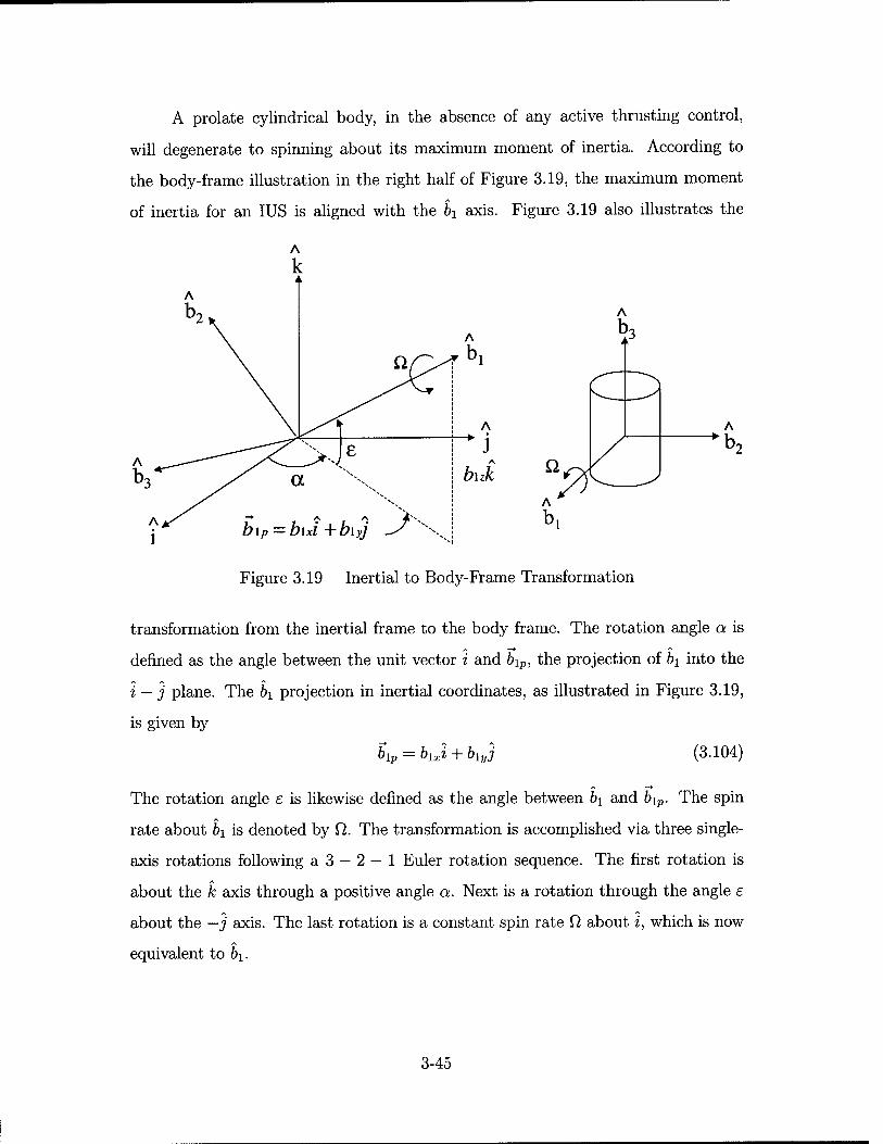
A prolate cylindrical body, in the absence of any active thrusting control,
will degenerate to spinning about its maximum moment of inertia. According to
the body-frame illustration in the right half of Figure 3.19, the maximum moment
of inertia for an IUS is aligned with the bi axis. Figure 3.19 also illustrates the
b\P = but +biyj -/ \
Figure 3.19 Inertial to Body-Frame Transformation
transformation from the inertial frame to the body frame. The rotation angle a is
defined as the angle between the unit vector i and b\p, the projection of b\ into the
i — j plane. The bi projection in inertial coordinates, as illustrated in Figure 3.19,
is given by
biP = hJ + blyj (3.104)
The rotation angle e is likewise defined as the angle between &i and b\v. The spin
rate about by is denoted by £). The transformation is accomplished via three single-
axis rotations following a 3 — 2 — 1 Euler rotation sequence. The first rotation is
about the k axis through a positive angle a. Next is a rotation through the angle e
about the —j axis. The last rotation is a constant spin rate £1 about i, which is now
equivalent to b\.
3-45
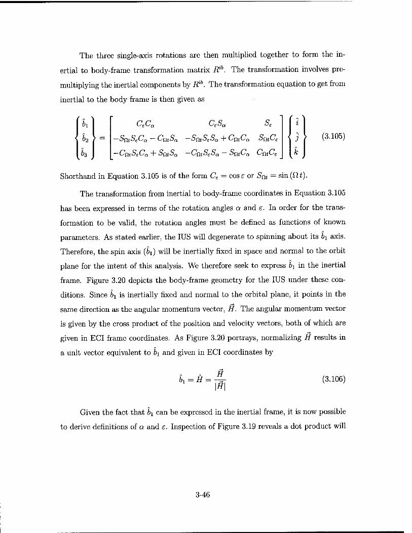
The three single-axis rotations are then multiplied together to form the in-
ertial to body-frame transformation matrix Rib. The transformation involves pre-
multiplying the inertial components by Rib. The transformation equation to get from
inertial to the body frame is then given as
C£Ca &e&a *->£
—SntSeCa — CatSa —ScitS£Sa + CatCa SmCe
— CfttSeCa + SfitSa —CntS£Sa — SntCa CatC£
( - x
i
j
k
(3.105)
Shorthand in Equation 3.105 is of the form Cs = cose or Snt = sin (Qt).
The transformation from inertial to body-frame coordinates in Equation 3.105
has been expressed in terms of the rotation angles a and e. In order for the trans-
formation to be valid, the rotation angles must be defined as functions of known
parameters. As stated earlier, the IUS will degenerate to spinning about its bi axis.
Therefore, the spin axis (Si) will be inertially fixed in space and normal to the orbit
plane for the intent of this analysis. We therefore seek to express bx in the inertial
frame. Figure 3.20 depicts the body-frame geometry for the IUS under these con-
ditions. Since Si is inertially fixed and normal to the orbital plane, it points in the
same direction as the angular momentum vector, H. The angular momentum vector
is given by the cross product of the position and velocity vectors, both of which are
given in ECI frame coordinates. As Figure 3.20 portrays, normalizing H results in
a unit vector equivalent to Si and given in ECI coordinates by
SI = H = 4- \H\
(3.106)
Given the fact that Si can be expressed in the inertial frame, it is now possible
to derive definitions of a and e. Inspection of Figure 3.19 reveals a dot product will
3-46
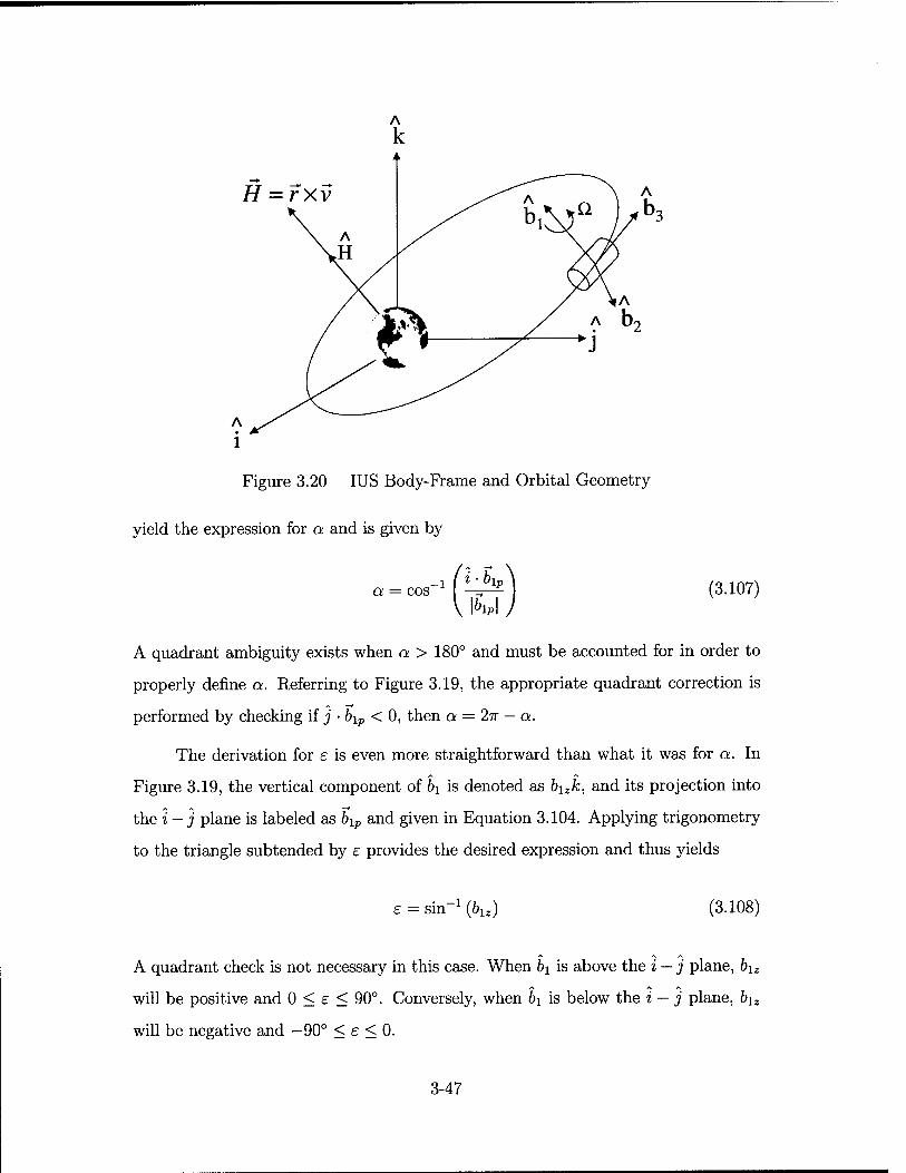
H = rxv
Figure 3.20 IUS Body-Frame and Orbital Geometry
yield the expression for a and is given by
a = cos -l i-b iP
M (3.107)
A quadrant ambiguity exists when a > 180° and must be accounted for in order to
properly define a. Referring to Figure 3.19, the appropriate quadrant correction is
performed by checking if j • 6lp < 0, then a = 2n — a.
The derivation for e is even more straightforward than what it was for a. In
Figure 3.19, the vertical component of b\ is denoted as bizk, and its projection into
the i—j plane is labeled as b\p and given in Equation 3.104. Applying trigonometry
to the triangle subtended by e provides the desired expression and thus yields
e = sin (blz) (3.108)
A quadrant check is not necessary in this case. When b\ is above the i — j plane, biz
will be positive and 0 < e < 90°. Conversely, when b\ is below the i — j plane, b\z
will be negative and —90° < e < 0.
3-47
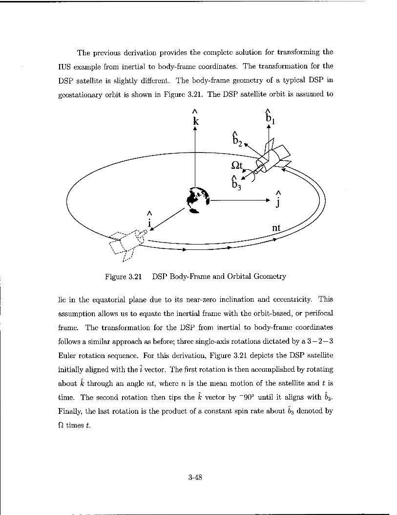
The previous derivation provides the complete solution for transforming the
IUS example from inertial to body-frame coordinates. The transformation for the
DSP satellite is slightly different. The body-frame geometry of a typical DSP in
geostationary orbit is shown in Figure 3.21. The DSP satellite orbit is assumed to
\..-V7
Figure 3.21 DSP Body-Frame and Orbital Geometry
lie in the equatorial plane due to its near-zero inclination and eccentricity. This
assumption allows us to equate the inertial frame with the orbit-based, or perifocal
frame. The transformation for the DSP from inertial to body-frame coordinates
follows a similar approach as before; three single-axis rotations dictated by a 3 —2 —3
Euler rotation sequence. For this derivation, Figure 3.21 depicts the DSP satellite
initially aligned with the i vector. The first rotation is then accomplished by rotating
about k through an angle nt, where n is the mean motion of the satellite and t is
time. The second rotation then tips the k vector by ~90° until it aligns with b3.
Finally, the last rotation is the product of a constant spin rate about b3 denoted by
D, times t.
3-48
The transformation equation for a DSP satellite to get from inertial to the
body frame is then given as
-ScitSnt SntCnt Cm
-CutSnt CntCnt —Seit
~Cnt —Snt 0
(3.109)
Shorthand in Equation 3.109 is also of the form as previously described.
Recall the objective of coordinate transformations in this section is to con-
vert the satellite-Sun vector (p) from inertial to body-frame coordinates. The ECI
coordinates of p are pre-multiplied by the transformation matrix R?b to obtain p in
body-frame coordinates. It is the body-frame form of p that is then incorporated into
the SRP force derivation. The SRP acceleration (ap) is then transformed back to the
inertial frame by pre-multiplying by the transpose of Rlb, denoted by (Rlb)T. Once
this is done, the equations of motion are numerically integrated to obtain new pre-
dictions of satellite position and velocity in ECI coordinates. The remainder of this
chapter describes the process of calculating residuals and subsequent comparative
analysis between the baseline model and the various SRP effects.
3.4 Calculating and Optimizing Residuals
The SRP model in this thesis will be simulated for the duration of one year.
A pre-defined set of classical orbital elements will be converted to initial position
and velocity of the satellite. These initial conditions will then be propagated via
numerical integration in accordance with equations of motion containing the SRP
model found in Equation 3.10. The numerical integrator uses a 5th/6th order Runge-
Kutta with variable step size and a tolerance of 10~12. Prior to simulating, it will
be possible to select from four separate flags that indicate which SRP effect should
be simulated. These simulation control flags include solar flux, area, coefficient of
reflection, and shadow effects. The solar flux flag will permit the user to choose
whether to model a constant or variable solar flux. Similarly, the area flag allows
3-49
the user to toggle between a constant or changing area of the satellite silhouette.
The coefficient of reflection flag switches from specular reflection to both specular
and diffuse reflection, and the shadow flag swaps between the cylindrical or conical
Earth shadow models.
The simulation will actually be performed twice. The first run of the simulation
will propagate the satellite in compliance with user defined flags previously discussed.
This simulation run will hereafter be referred to as the truth model. Satellite position
and velocity at each time step will be archived for subsequent data analysis. The
second simulation run will incorporate the baseline model as derived earlier in the
chapter and will adopt the same name. Recall the baseline model consists of a
variable solar flux, constant area, specular reflection and a cylindrical Earth shadow
model. The second run will also output the satellite position and velocity at each
simulated time step. The two models may further be differentiated in that the truth
model will typically be more complex due to the additional SRP effects, and thus
consumes more computation time.
The objective is to now perform a comparative analysis on the output of the
truth and baseline models, for the purpose of evaluating the merits of modeling higher
order SRP effects as outlined in Section 1.4. This is accomplished by first calculating
residuals at each simulated time step. A residual is defined as the difference between
the actual observed value of some data point, and a prediction of the same point.
Likewise, a residual in this thesis will be defined as the difference between a positional
data point in the truth model, and the corresponding data point from the baseline.
The result will be an array of satellite position residuals computed at 100 second
time increments over the course of one year. In essence, each residual describes how
far off in satellite position, the baseline model is from the truth model at one instant
in time. This data array must now be mathematically summarized in order to assign
some physical dimension to the year-long simulation.
3-50
The function of choice to compress the year's worth of data is the root-mean-
square (RMS). Equation 3.110 illustrates the computation of the RMS vector where
N is the number of time steps.
r> T\ /r q _ , / L^i=\ V truth f baseline) (3 110)
The RMS is a vector at this point in time because the satellite position is a vector.
The RMS first squares each residual and then sums them up. Next, the sum of
the squares is averaged by dividing by the total number of simulation steps. This
mean value is finally square-rooted to obtain the final RMS value. The RMS now
represents the overall variation in satellite position between the truth and baseline
models. It should be obvious that in the final analysis, the lower the RMS, the closer
the truth and baseline models are to each other in modeling SRR Depending on the
acceptable level of prediction accuracy, a low RMS may indicate that use of the
truth model is not warranted, and hence computation time reduced by employing
the baseline.
Recall the position and velocity of the satellite at each time step are output in
ECI coordinates. The calculated RMS is therefore also in ECI coordinates. However,
the ECI frame does not impart the proper physicality one needs in describing the
relative difference in positions of the satellite, as predicted by the truth and baseline
models. It would be more beneficial to describe the RMS in relative terms of radial,
in-track and cross-track components of one of the models, for example the baseline.
This may be achieved by transforming the RMS from inertial to a frame rotating
with the satellite (fOz). The transformation from inertial (ijk) to (f6z) may be
realized by populating a transformation matrix with the inertial frame components
of {r0 z). The position vector of a satellite in the baseline is already given in ECI
coordinates. The unit vector f may thus be obtained by
r = ^ (3.111) In
3-51
The cross-track component z is normal to the orbital plane and thus aligned with
the angular momentum vector H. The unit vector z is then given by
z = t = ^ (3.112) \H\ \rxv\
The third member of the (f 9 z) frame is orthogonal to both z and f, and thus defined
by their cross product and expressed as
§ = zxf (3.113)
All three components of the (f 9 z) frame are now given in ECI coordinates. The
transformation from (i j k) to (f 9 z) coordinates is denoted by RlT and consequently
derived as n r2 r3
Rir= 0! e2 e3 (3.H4)
Z\ 22 z3
Pre-multiplying the RMS by the transformation Rir yields an RMS vector in
terms of radial, in-track and cross-track components rooted in the baseline. The
total magnitude of this vector is given by
RMS = ^RMSf + RMSi + RMSl (3.115)
The scalar RMS value of Equation 3.115 now represents the overall relative distance
separating the predictions of the truth and baseline models after one year of simu-
lation. As previously stated, the smaller the RMS, the closer the truth and baseline
are in propagating the satellite to essentially the same point in space. This case
would indicate that the additional modeling complexity is not warranted. A larger
RMS however, may justify the use of the truth model. One would obviously prefer
the baseline model over the truth model if the RMS could be driven to an acceptably
small enough value. The process that follows is known as optimizing residuals.
3-52
The baseline model contains variables or constants that have an impact on the
predicted satellite position, and therefore impact the value of the RMS. Some of these
variables and constants include the radius of the Earth (R®), effective satellite area
in the form of a flat plate (A), coefficient of reflection (ß), and solar flux constant
($o). The first of these, RQ, is employed in the baseline satellite illumination test
case found in Equation 3.36. The latter three, A, ß, and $0) are primary components
of the baseline model described in Equation 3.30. The RMS may thus be adjusted
somewhat by changing the values of the variables and constants in the baseline.
The objective is to iteratively change these values until a minimum value of RMS is
obtained. Ironically, some of the so-called constants are in fact not precisely known
and are subsequently solved for in the OD process. The residuals calculated in
this manner are therefore more representative of the OD process for which the SRP
model will be used, than the residuals computed when the constants are assumed
to be constant. In essence, this method of calculating and optimizing residuals
functionally mimics the results that one would obtain from an OD filter.
In order to optimize residuals, the baseline model must be iteratively simulated,
changing a selected variable or constant at each iteration, until the minimum RMS is
obtained. When the RMS passes a pre-defined convergence test, the simulation ends
and the RMS, as well as the final value of the variable or constant that was iteratively
changed, are output. If the RMS is at an acceptable level, the conclusion is that the
baseline model is preferred, given the final value of the constant or variable that was
iteratively changed. Otherwise, the new modeling effect in the truth model should
be included to improve OD accuracies. Many optimization techniques exist that may
be employed to minimize the RMS. The method of choice in this simulation is the
Golden Section Search algorithm in one dimension and can be found in Numerical
Recipes by Press et al [26]. Analysis and results of several simulation runs of this
type are found in the next chapter.
3-53
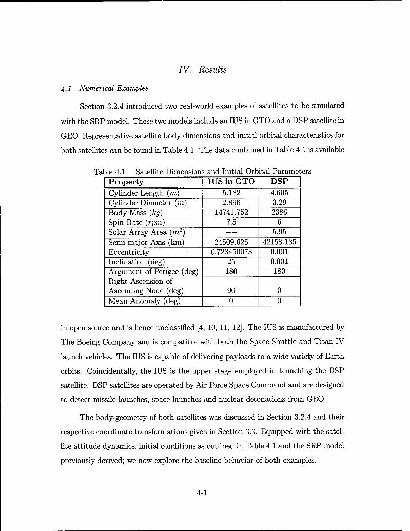
IV. Results
4-1 Numerical Examples
Section 3.2.4 introduced two real-world examples of satellites to be simulated
with the SRP model. These two models include an IUS in GTO and a DSP satellite in
GEO. Representative satellite body dimensions and initial orbital characteristics for
both satellites can be found in Table 4.1. The data contained in Table 4.1 is available
Table 4.1 Satellite Dimensions and Initial Orbital Parameters Property IUS in GTO DSP
Cylinder Length (TO) 5.182 4.605 Cylinder Diameter (TO) 2.896 3.29 Body Mass (kg) 14741.752 2386 Spin Rate (rpm) 7.5 6 Solar Array Area (m2) — 5.95 Semi-major Axis (km) 24509.625 42158.135 Eccentricity 0.723450073 0.001 Inclination (deg) 25 0.001 Argument of Perigee (deg) 180 180 Right Ascension of Ascending Node (deg) 90 0 Mean Anomaly (deg) 0 0
in open source and is hence unclassified [4, 10, 11, 12]. The IUS is manufactured by
The Boeing Company and is compatible with both the Space Shuttle and Titan IV
launch vehicles. The IUS is capable of delivering payloads to a wide variety of Earth
orbits. Coincidentally, the IUS is the upper stage employed in launching the DSP
satellite. DSP satellites are operated by Air Force Space Command and are designed
to detect missile launches, space launches and nuclear detonations from GEO.
The body-geometry of both satellites was discussed in Section 3.2.4 and their
respective coordinate transformations given in Section 3.3. Equipped with the satel-
lite attitude dynamics, initial conditions as outlined in Table 4.1 and the SRP model
previously derived; we now explore the baseline behavior of both examples.
4-1
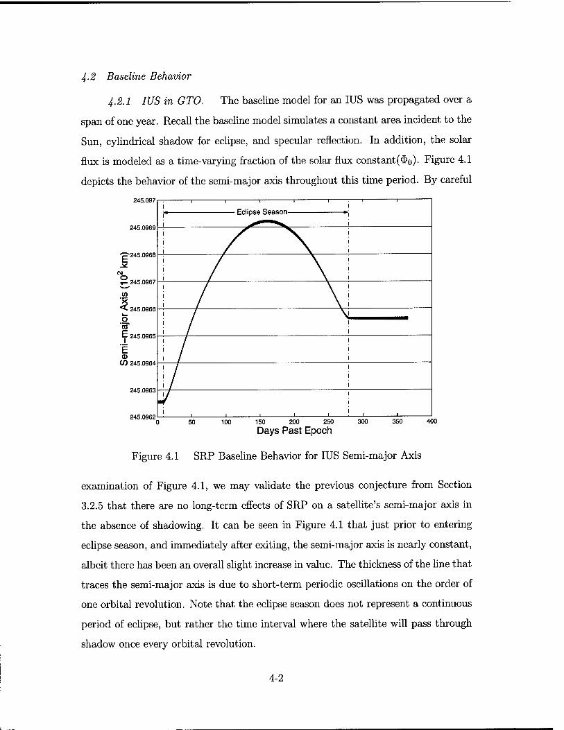
4-2 Baseline Behavior
4.2.1 IUS in GTO. The baseline model for an IUS was propagated over a
span of one year. Recall the baseline model simulates a constant area incident to the
Sun, cylindrical shadow for eclipse, and specular reflection. In addition, the solar
flux is modeled as a time-varying fraction of the solar flux constant($0). Figure 4.1
depicts the behavior of the semi-major axis throughout this time period. By careful
245.097
245.0969
-p-245.0968
CM
■P- 245.0967
245.0966 3 o 'or E 245.0965
1 CO 245.0964
245.0963
245.0962
_ ! r , , 1 . 1 1
! f \ i ! / \ !
I / \: / \i
; / ;
I / ; \ I
! 1 1 1 1 11 1
50 100 150 200 250
Days Past Epoch 300 350 400
Figure 4.1 SRP Baseline Behavior for IUS Semi-major Axis
examination of Figure 4.1, we may validate the previous conjecture from Section
3.2.5 that there are no long-term effects of SRP on a satellite's semi-major axis in
the absence of shadowing. It can be seen in Figure 4.1 that just prior to entering
eclipse season, and immediately after exiting, the semi-major axis is nearly constant,
albeit there has been an overall slight increase in value. The thickness of the line that
traces the semi-major axis is due to short-term periodic oscillations on the order of
one orbital revolution. Note that the eclipse season does not represent a continuous
period of eclipse, but rather the time interval where the satellite will pass through
shadow once every orbital revolution.
4-2
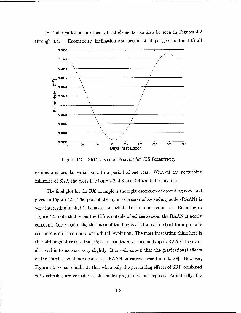
Periodic variation in other orbital elements can also be seen in Figures 4.2
through 4.4. Eccentricity, inclination and argument of perigee for the IUS all
72.3452
72.345
50 100 150 200 250
Days Past Epoch 300 350 400
Figure 4.2 SRP Baseline Behavior for IUS Eccentricity
exhibit a sinusoidal variation with a period of one year. Without the perturbing
influence of SRP, the plots in Figure 4.2, 4.3 and 4.4 would be flat lines.
The final plot for the IUS example is the right ascension of ascending node and
given in Figure 4.5. The plot of the right ascension of ascending node (RAAN) is
very interesting in that it behaves somewhat like the semi-major axis. Referring to
Figure 4.5, note that when the IUS is outside of eclipse season, the RAAN is nearly
constant. Once again, the thickness of the line is attributed to short-term periodic
oscillations on the order of one orbital revolution. The most interesting thing here is
that although after entering eclipse season there was a small dip in RAAN, the over-
all trend is to increase very slightly. It is well known that the gravitational effects
of the Earth's oblateness cause the RAAN to regress over time [9, 38]. However,
Figure 4.5 seems to indicate that when only the perturbing effects of SRP combined
with eclipsing are considered, the nodes progress versus regress. Admittedly, the
4-3
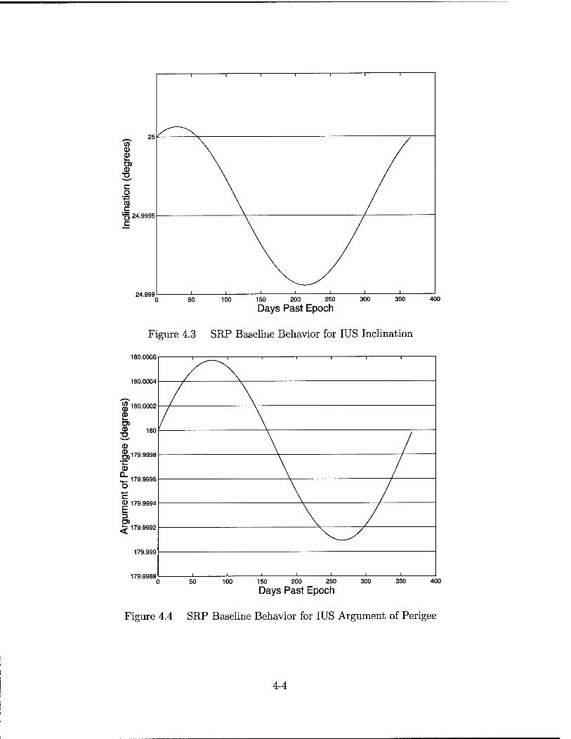
24.999 400
Days Past Epoch
Figure 4.3 SRP Baseline Behavior for IUS Inclination
180.0006
0)
^_ 179.9996 O
Cg 179.9994
3
^p 179.9992
179.999
179.9988 400
Days Past Epoch
Figure 4.4 SRP Baseline Behavior for IUS Argument of Perigee
4-4
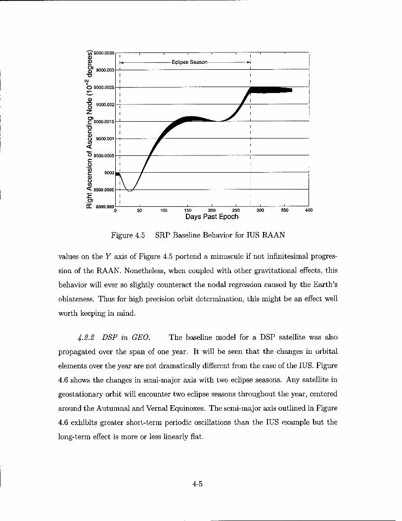
ffl 3000.0035 <D <1> L. U) (11 9000.003 T3
OJ
O 9000.0025 T" *^* a> U o 9000.002
C 9000.0015 T3 C
O 9000.001 OT < t o 3000.0005 c o (0 c 9000 a) u (0 < 3999.9995 ■•-» n u>
CC 8999.999
, , , 1 T. ■ | I I
^^~~ y f /
/
"N / i i i i .I i
50 100 150 200 250
Days Past Epoch 300 350 400
Figure 4.5 SRP Baseline Behavior for IUS RAAN
values on the Y axis of Figure 4.5 portend a minuscule if not infinitesimal progres-
sion of the RAAN. Nonetheless, when coupled with other gravitational effects, this
behavior will ever so slightly counteract the nodal regression caused by the Earth's
oblateness. Thus for high precision orbit determination, this might be an effect well
worth keeping in mind.
4-2.2 DSP in GEO. The baseline model for a DSP satellite was also
propagated over the span of one year. It will be seen that the changes in orbital
elements over the year are not dramatically different from the case of the IUS. Figure
4.6 shows the changes in semi-major axis with two eclipse seasons. Any satellite in
geostationary orbit will encounter two eclipse seasons throughout the year, centered
around the Autumnal and Vernal Equinoxes. The semi-major axis outlined in Figure
4.6 exhibits greater short-term periodic oscillations than the IUS example but the
long-term effect is more or less linearly flat.
4-5
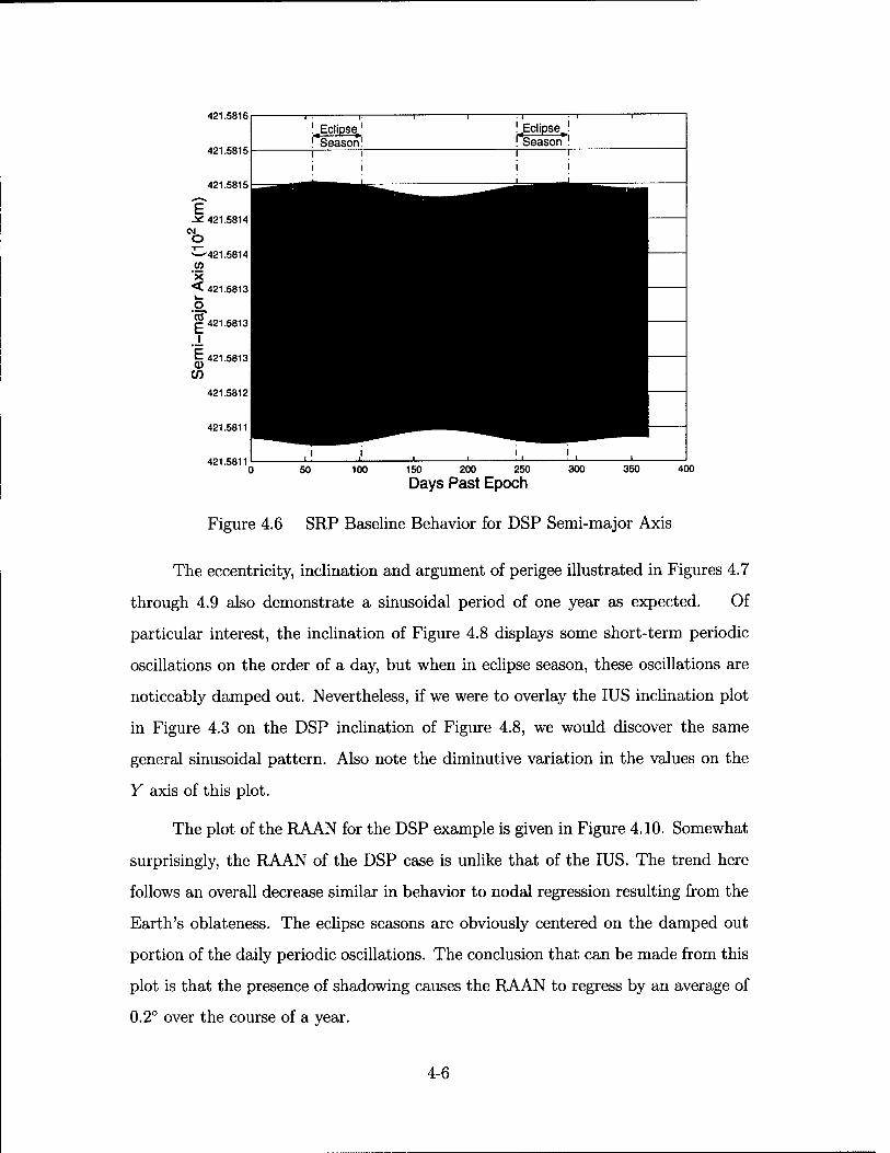
421.5816
421.5815
50 100 150 200 250
Days Past Epoch 300 350 400
Figure 4.6 SRP Baseline Behavior for DSP Semi-major Axis
The eccentricity, inclination and argument of perigee illustrated in Figures 4.7
through 4.9 also demonstrate a sinusoidal period of one year as expected. Of
particular interest, the inclination of Figure 4.8 displays some short-term periodic
oscillations on the order of a day, but when in eclipse season, these oscillations are
noticeably damped out. Nevertheless, if we were to overlay the IUS inclination plot
in Figure 4.3 on the DSP inclination of Figure 4.8, we would discover the same
general sinusoidal pattern. Also note the diminutive variation in the values on the
Y axis of this plot.
The plot of the RAAN for the DSP example is given in Figure 4.10. Somewhat
surprisingly, the RAAN of the DSP case is unlike that of the IUS. The trend here
follows an overall decrease similar in behavior to nodal regression resulting from the
Earth's oblateness. The eclipse seasons are obviously centered on the damped out
portion of the daily periodic oscillations. The conclusion that can be made from this
plot is that the presence of shadowing causes the RAAN to regress by an average of
0.2° over the course of a year.
4-6
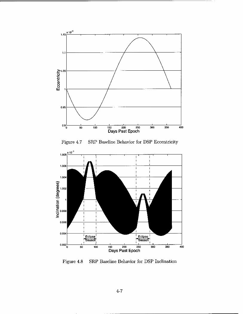
1.15 xicr
50 100 150 200 250 300 350 400
Days Past Epoch
Figure 4.7 SRP Baseline Behavior for DSP Eccentricity
1.008
1.006
1.004
"v> CD 2 1.002 O) CD ■a
,o CO
■M 0.998 Ü C
0.996
0.994
0.992
x10' r^ 1 1— i i -i i
^/VA^ A
^V1^^^. ■ ■ A ^V ^^^^ A ^1 ^r ' ^^^^■r^^l r • ' ^^^H ^^1
^^ ^^i i^B ^r
Eclipse Eclipse ! Reason! '"Season!
. ' i , , ! . ' . 50 100 150 200 250 300 350 400
Days Past Epoch
Figure 4.8 SRP Baseline Behavior for DSP Inclination
4-7
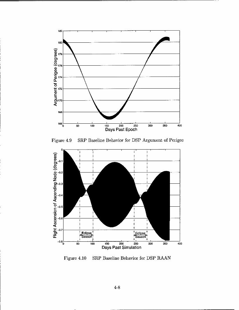
400
Days Past Epoch
Figure 4.9 SRP Baseline Behavior for DSP Argument of Perigee
CO © 0 £-0.1 O) CD ;o CU-0.2
T3 O
O>-0.3 c
8-0.4 tn < w-0.5 c o
'co © -0.6 O CO <
-0.7
-0.8
^ n 1.— i i - i -i i
^k ■ .^^^. ■ ^A j^^^^k :^fl ^V^^^^^L^^I ^r ^^^^B^^^l W\ ^^^^r[ ^^1 :^^^ : ^H
^Eclipse! ! Eclipse^' ^B !*Season! Reason! ^H
50 100 150 200 250 300
Days Past Simulation 350 400
Figure 4.10 SRP Baseline Behavior for DSP RAAN
4-8
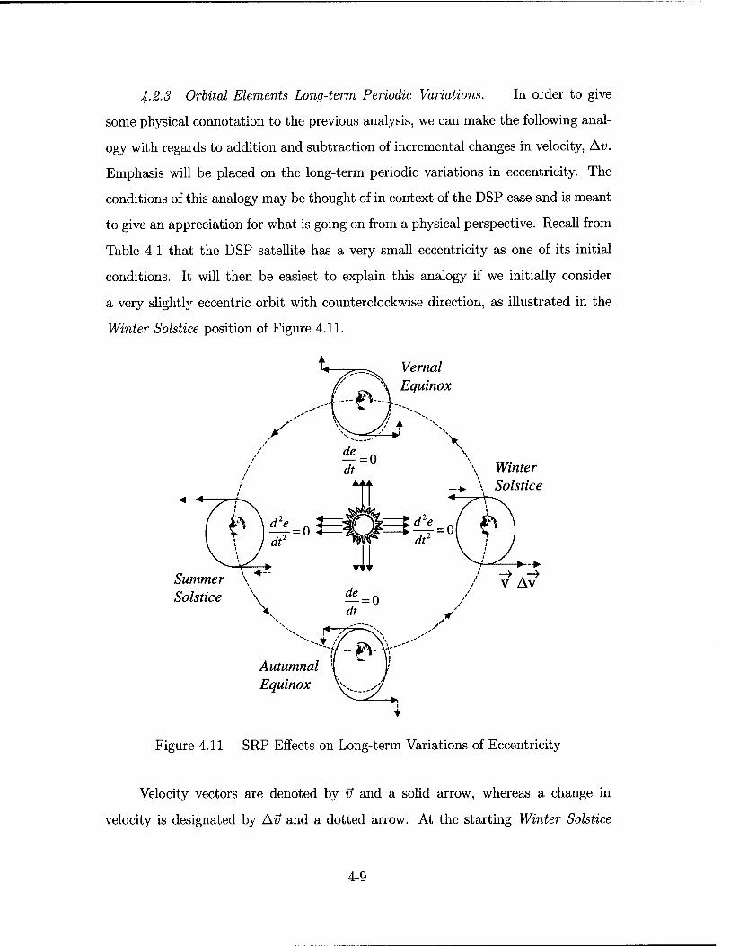
4-2.3 Orbital Elements Long-term Periodic Variations. In order to give
some physical connotation to the previous analysis, we can make the following anal-
ogy with regards to addition and subtraction of incremental changes in velocity, Av.
Emphasis will be placed on the long-term periodic variations in eccentricity. The
conditions of this analogy may be thought of in context of the DSP case and is meant
to give an appreciation for what is going on from a physical perspective. Recall from
Table 4.1 that the DSP satellite has a very small eccentricity as one of its initial
conditions. It will then be easiest to explain this analogy if we initially consider
a very slightly eccentric orbit with counterclockwise direction, as illustrated in the
Winter Solstice position of Figure 4.11.
Vernal _ , Equinox
Winter Solstice
<-<
Summer Solstice
Autumnal Equinox
Figure 4.11 SRP Effects on Long-term Variations of Eccentricity
Velocity vectors are denoted by v and a solid arrow, whereas a change in
velocity is designated by Av and a dotted arrow. At the starting Winter Solstice
4-9
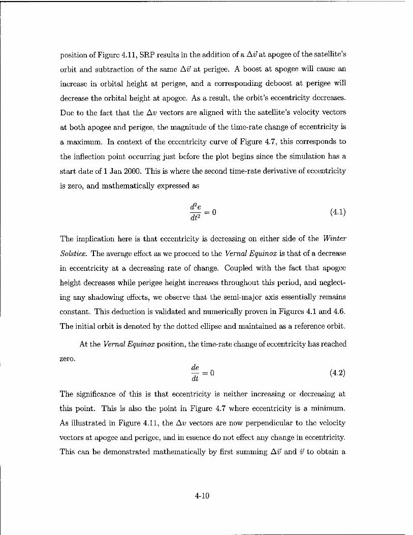
position of Figure 4.11, SRP results in the addition of a Av at apogee of the satellite's
orbit and subtraction of the same Av at perigee. A boost at apogee will cause an
increase in orbital height at perigee, and a corresponding deboost at perigee will
decrease the orbital height at apogee. As a result, the orbit's eccentricity decreases.
Due to the fact that the Av vectors are aligned with the satellite's velocity vectors
at both apogee and perigee, the magnitude of the time-rate change of eccentricity is
a maximum. In context of the eccentricity curve of Figure 4.7, this corresponds to
the inflection point occurring just before the plot begins since the simulation has a
start date of 1 Jan 2000. This is where the second time-rate derivative of eccentricity
is zero, and mathematically expressed as
The implication here is that eccentricity is decreasing on either side of the Winter
Solstice. The average effect as we proceed to the Vernal Equinox is that of a decrease
in eccentricity at a decreasing rate of change. Coupled with the fact that apogee
height decreases while perigee height increases throughout this period, and neglect-
ing any shadowing effects, we observe that the semi-major axis essentially remains
constant. This deduction is validated and numerically proven in Figures 4.1 and 4.6.
The initial orbit is denoted by the dotted ellipse and maintained as a reference orbit.
At the Vernal Equinox position, the time-rate change of eccentricity has reached
zero.
I- M The significance of this is that eccentricity is neither increasing or decreasing at
this point. This is also the point in Figure 4.7 where eccentricity is a minimum.
As illustrated in Figure 4.11, the Av vectors are now perpendicular to the velocity
vectors at apogee and perigee, and in essence do not effect any change in eccentricity.
This can be demonstrated mathematically by first summing Av and v to obtain a
4-10
resultant vector which we will call vnew, and in which the magnitude is given by
vnew = Vv* + Av2 (4.3)
Factoring out a v2 under the radical and bringing it to the outside yields
= *V1+lv)2 (4'4)
Equation 4.4 may be approximated by a binomial series expansion which would then
result in , 1 fAv\2 1 (Av\4 .. cx 1 + 2(vj -B{T)
+'"\ (45)
It should be immediately apparent that since the terms containing Av are higher
order expressions, the orbital eccentricity contribution of Av is effectively nil at
apogee and perigee. The significance of this conclusion is once again that eccentricity
is a minimum and its time-rate of change is zero at the Vernal Equinox. This analysis
is further supported by the DSP plots in Section 4.2.2. Recall from Section 4.2.2 that
an equinox is coincidental to an eclipse season for the DSP satellite. The first eclipse
season depicted in Figure 4.8 is associated with the Vernal Equinox and corresponds
to the minimum value of the eccentricity curve given in Figure 4.7.
At the Summer Solstice position, the At; vectors align with the velocity vectors
at apogee and perigee, thereby once again making their greatest impact on the
eccentric changes in the orbit. The addition of a Av at apogee and subtraction of
the same Av at perigee, now has the opposite effect that it did at Winter Solstice.
The extra kick at perigee will now increase apogee height and the deboost at apogee
will decrease perigee height. Thus, contrary to the Winter Solstice scenario, the
inference is that eccentricity is increasing on either side of Summer Solstice. To be
precise, from the Vernal Equinox to Summer Solstice, eccentricity is increasing at
an increasing rate of change, and from Summer Solstice to the Autumnal Equinox,
eccentricity is increasing at a decreasing rate of change.
4-11
Analogous to the Vernal Equinox scenario, the time-rate change of eccentricity
at the Autumnal Equinox is once again zero for the same reasons as previously
discussed. In contrast however, this zero time-rate of change was arrived at from
the increasing side of eccentricity versus the decreasing side. The import of this
conclusion is that eccentricity is now at a maximum. The Autumnal Equinox is
associated with the second eclipse season depicted in Figure 4.8 and corresponds to
the maximum value of the eccentricity curve given in Figure 4.7. As time progresses
back to the Winter Solstice, eccentricity begins to decrease at an increasing rate, until
the magnitude of the time-rate change of eccentricity again reaches a maximum and
the cycle begins again. In summary, eccentricity increases over a six month period
from Vernal Equinox to Autumnal Equinox, and decreases over the following six
month period back to Vernal Equinox. The conclusions of this analogy may be
verified by close inspection of Figure 4.7.
As previously mentioned, this analogy was presented in terms of long-term
periodic variations in eccentricity. Similar long-term periodic variations occur in
inclination and argument of perigee, as depicted in their corresponding plots found
in Sections 4.2.1 and 4.2.2. The semi-major axis and right ascension of ascending
node essentially remain constant throughout this analogy if shadowing effects are
neglected; a conjecture thus supported by their corresponding plots also found in
Sections 4.2.1 and 4.2.2.
Thus far, the results have only included the behavior of the baseline model and
the resulting variation in the orbital elements. This sets the stage for the next phase
of analysis. While it is interesting to note the change in orbital parameters, the main
objective is to increase OD accuracy through modeling of higher order SRP effects.
Since the basic shape of the plots relating to the variation in orbital elements does
not radically change when other SRP effects are modeled, these plots will not be
reproduced for each effect.
4-12
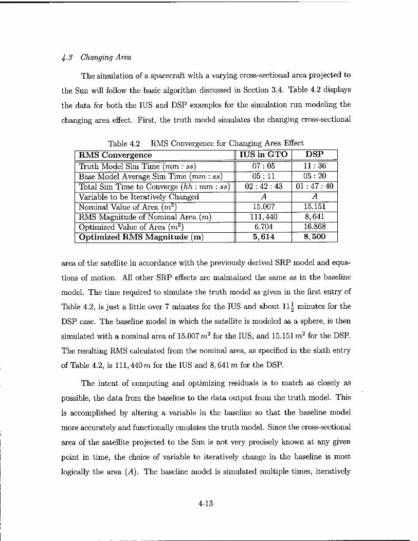
4-3 Changing Area
The simulation of a spacecraft with a varying cross-sectional area projected to
the Sun will follow the basic algorithm discussed in Section 3.4. Table 4.2 displays
the data for both the IUS and DSP examples for the simulation run modeling the
changing area effect. First, the truth model simulates the changing cross-sectional
Table 4.2 RMS Convergence for Changing Area Effect
RMS Convergence IUS in GTO DSP
Truth Model Sim Time (mm : ss) 07:05 11:36 Base Model Average Sim Time (mm : ss) 05: 11 05:20 Total Sim Time to Converge (hh : mm : ss) 02 : 42 : 43 01 : 47 : 40 Variable to be Iteratively Changed A A Nominal Value of Area (m2) 15.007 15.151 RMS Magnitude of Nominal Area (m) 111,440 8,641 Optimized Value of Area (TO
2) 6.704 16.868
Optimized RMS Magnitude (m) 5,614 8,500
area of the satellite in accordance with the previously derived SRP model and equa-
tions of motion. All other SRP effects are maintained the same as in the baseline
model. The time required to simulate the truth model as given in the first entry of
Table 4.2, is just a little over 7 minutes for the IUS and about 111 minutes for the
DSP case. The baseline model in which the satellite is modeled as a sphere, is then
simulated with a nominal area of 15.007 m2 for the IUS, and 15.151 m2 for the DSP.
The resulting RMS calculated from the nominal area, as specified in the sixth entry
of Table 4.2, is 111, 440m for the IUS and 8,641 TO for the DSP.
The intent of computing and optimizing residuals is to match as closely as
possible, the data from the baseline to the data output from the truth model. This
is accomplished by altering a variable in the baseline so that the baseline model
more accurately and functionally emulates the truth model. Since the cross-sectional
area of the satellite projected to the Sun is not very precisely known at any given
point in time, the choice of variable to iteratively change in the baseline is most
logically the area (A). The baseline model is simulated multiple times, iteratively
4-13
changing the value of A until RMS convergence is achieved. The average time to
simulate the baseline on one iteration is just a little over 5 minutes in both examples.
Line three of Table 4.2 indicates the total simulation time required to reach RMS
convergence is on the order of a couple of hours. Each subsequent iteration of the
baseline simulation adjusts the value of A in accordance with the Golden Section
Search algorithm [26]. The bounds on A for the Golden Section Search algorithm
are set to [A/A, 2 A] and denote a range from one-fourth the nominal A to twice that
value. The convergence tolerance is set at 0.001 m, which implies the simulation will
continue until consecutive iterations yield a difference in RMS less than or equal to
0.001m.
The optimized value of A, or in other words the value of A that yields the
smallest residuals, is given in Table 4.2 as 6.704 TO2 for the IUS, and 16.868 m2 for
the DSP case. These optimized values for A result in convergence and an optimized
RMS value of 5,614 m and 8,500 m for the IUS and DSP respectively. One can
quickly observe that the optimized value of A, considerably outperforms the nominal
value by at least 105 km in the IUS case and by only 140 m in the DSP case. The
interpretation of the optimized RMS magnitude is that if the optimized value of area
is employed, it will functionally imitate the manner in which residuals are derived
if the satellite area is included as a solve-for parameter in an OD filter. In the
case of the IUS, after one year the baseline prediction will diverge from the truth
model by about 5.6 km. The residuals calculated within an actual OD filter would
be presumably smaller than what was calculated here, and is hence a topic of future
work in Section 5.2. The interpretation of the optimized RMS in the DSP case is
made in like fashion. Compared to the RMS magnitudes of other effects yet to be
presented, the changing area effect seems to have the greatest impact on OD and
should be a concern for precise navigation. The implication for the effect of changing
area is that the baseline model is probably not sufficient for OD, albeit computation
time is much shorter.
4-14
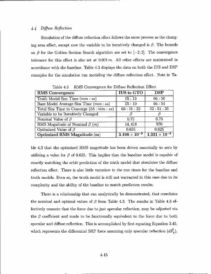
4-4 Diffuse Reflection
Simulation of the diffuse reflection effect follows the same process as the chang-
ing area effect, except now the variable to be iteratively changed is ß. The bounds
on ß for the Golden Section Search algorithm are set to [-2,2]. The convergence
tolerance for this effect is also set at 0.001m. All other effects are maintained in
accordance with the baseline. Table 4.3 displays the data on both the IUS and DSP
examples for the simulation run modeling the diffuse reflection effect. Note in Ta-
Table 4.3 RMS Convergence for Diffuse Reflection Effect
RMS Convergence IUS in GTO DSP
Truth Model Sim Time (mm : ss) 05:13 04:56 Base Model Average Sim Time (mm : ss) 05: 10 04:54 Total Sim Time to Converge (hh : mm : ss) 03 : 21 : 22 02 : 51 : 35 Variable to be Iteratively Changed ß ß Nominal Value of ß 0.75 0.75 RMS Magnitude of Nominal ß (m) 14,418 970 Optimized Value of ß 0.625 0.625 Optimized RMS Magnitude (m) 3.198 x 10"3 1.331 x 10~3
ble 4.3 that the optimized RMS magnitude has been driven essentially to zero by
utilizing a value for ß of 0.625. This implies that the baseline model is capable of
exactly matching the orbit prediction of the truth model that simulates the diffuse
reflection effect. There is also little variation in the run times for the baseline and
truth models. Even so, the truth model is still not warranted in this case due to its
complexity and the ability of the baseline to match prediction results.
There is a relationship that can analytically be demonstrated, that correlates
the nominal and optimal values of ß from Table 4.3. The results in Table 4.3 ef-
fectively connote that the force due to just specular reflection, may be adjusted via
the ß coefficient and made to be functionally equivalent to the force due to both
specular and diffuse reflection. This is accomplished by first equating Equation 3.45,
which represents the differential SRP force assuming only specular reflection (dFp),
4-15
and Equation 3.63 which models both specular and diffuse reflection (dF).
dFp = dF (4.6)
Doing away with the vector notation and dividing out all common terms from both
sides results in
(1 - ß) + 2/? cos 6 = 2Sß cos 6 + (l-6)ßl + {l- 8ß) (4.7)
Since the baseline models the satellite as a sphere, it also assumes 6 — 0. Making
this substitution in Equation 4.7 and after some algebraic simplification, we get the
relationship
ß=\{2 + 5)ß (4.8)
The ß on the left side of this equation comes from dFp, and is representative of the ß
used in the baseline. Equation 4.8 then implies that if the baseline were to append a
factor of | (2 + 6) to its ß, it would produce the same results as the truth model, as
long as this is the only SRP effect being modeled. Note that the factor to multiply ß
by is a function of 6. For both IUS and DSP simulation cases summarized in Table
4.3, 8 assumed a value of |, which from Equation 4.8 yields a multiplicative factor
of |. The optimized value for ß is simply the product of the nominal value, given as
0.75 in Table 4.3, and the | factor. Performing this math yields an optimized value
for ß of 0.625, which is consistent with the numerical results of Table 4.3. Both the
factor and optimized value of ß will take on different magnitudes depending on the
assumed value of 6. Nevertheless, the conclusion is the same. The truth model is
not warranted in the case of diffuse reflection.
4-5 Conical Eclipse
Simulation results for the conical eclipse effect may be found in Table 4.4. The
key variable to iterate on for this effect is the radius of the Earth (i?©), with search
4-16
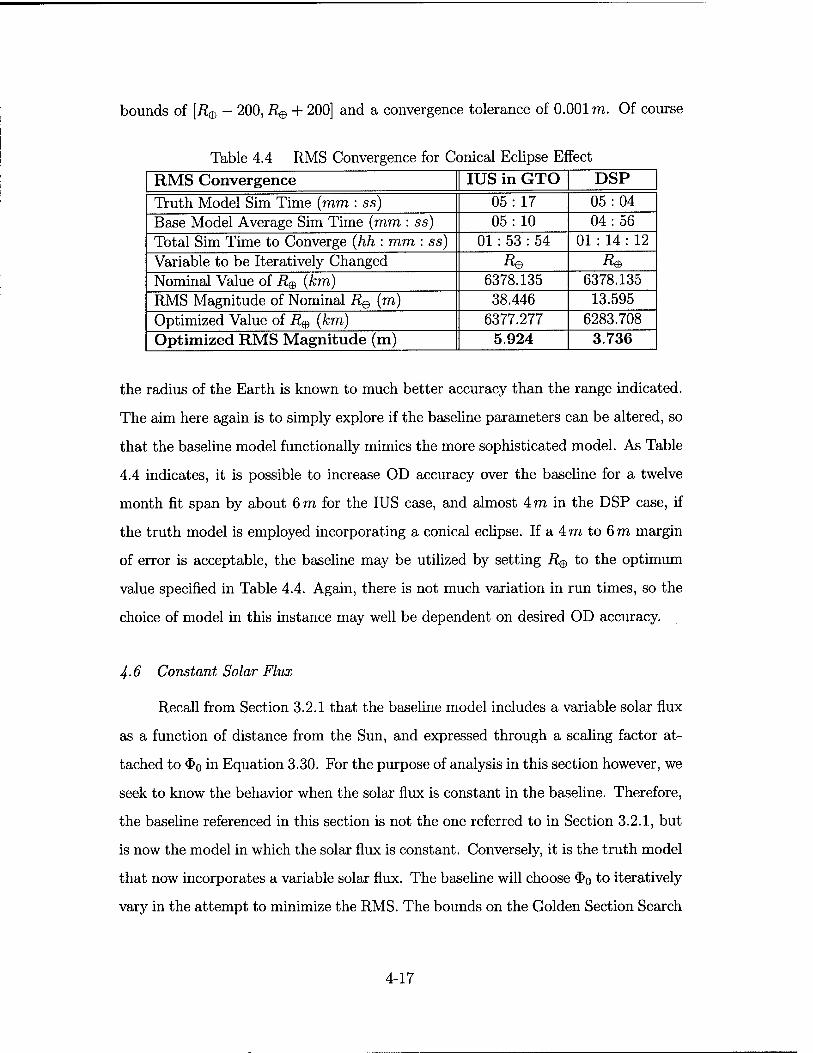
bounds of [Re - 200, i?e + 200] and a convergence tolerance of 0.001 m. Of course
Table 4.4 RMS Convergence for Conical Eclipse Effect
RMS Convergence IUS in GTO DSP
Truth Model Sim Time (mm : ss) 05: 17 05:04 Base Model Average Sim Time (mm : ss) 05: 10 04:56 Total Sim Time to Converge (hh : mm : ss) 01 : 53 : 54 01 : 14 : 12 Variable to be Iteratively Changed R® ■R®
Nominal Value of i?e (km) 6378.135 6378.135 RMS Magnitude of Nominal R® (m) 38.446 13.595 Optimized Value of R9 (km) 6377.277 6283.708 Optimized RMS Magnitude (m) 5.924 3.736
the radius of the Earth is known to much better accuracy than the range indicated.
The aim here again is to simply explore if the baseline parameters can be altered, so
that the baseline model functionally mimics the more sophisticated model. As Table
4.4 indicates, it is possible to increase OD accuracy over the baseline for a twelve
month fit span by about 6 m for the IUS case, and almost 4 m in the DSP case, if
the truth model is employed incorporating a conical eclipse. If a 4 TO to 6 TO margin
of error is acceptable, the baseline may be utilized by setting R® to the optimum
value specified in Table 4.4. Again, there is not much variation in run times, so the
choice of model in this instance may well be dependent on desired OD accuracy.
4-6 Constant Solar Flux
Recall from Section 3.2.1 that the baseline model includes a variable solar flux
as a function of distance from the Sun, and expressed through a scaling factor at-
tached to $o hi Equation 3.30. For the purpose of analysis in this section however, we
seek to know the behavior when the solar flux is constant in the baseline. Therefore,
the baseline referenced in this section is not the one referred to in Section 3.2.1, but
is now the model in which the solar flux is constant. Conversely, it is the truth model
that now incorporates a variable solar flux. The baseline will choose <&o to iteratively
vary in the attempt to minimize the RMS. The bounds on the Golden Section Search
4-17
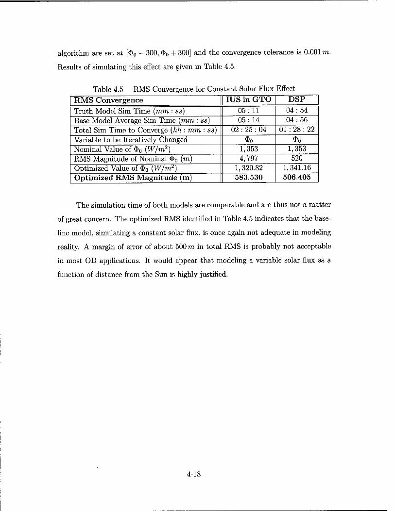
algorithm are set at [$0 - 300, $0 + 300] and the convergence tolerance is 0.001 m.
Results of simulating this effect are given in Table 4.5.
Table 4.5 RMS Convergence for Constant Solar Flux Effect
RMS Convergence IUS in GTO DSP
Truth Model Sim Time (mm : ss) 05: 11 04:54 Base Model Average Sim Time (mm : ss) 05: 14 04:56 Total Sim Time to Converge (hh : mm : ss) 02 : 25 : 04 01 : 28 : 22 Variable to be Iteratively Changed $o $0
Nominal Value of $0 (W/m2) 1,353 1,353 RMS Magnitude of Nominal $0 (m) 4,797 520 Optimized Value of <&0 (W/m2) 1,320.82 1,341.16 Optimized RMS Magnitude (m) 583.530 506.405
The simulation time of both models are comparable and are thus not a matter
of great concern. The optimized RMS identified in Table 4.5 indicates that the base-
line model, simulating a constant solar flux, is once again not adequate in modeling
reality. A margin of error of about 500 m in total RMS is probably not acceptable
in most OD applications. It would appear that modeling a variable solar flux as a
function of distance from the Sun is highly justified.
4-18
V. Conclusion
5.1 Summary and Recommendations
This research has shown that SRP is a significant enough non-gravitational
perturbation, that it cannot be ignored in the OD process. The specific effects of
SRP that may be modeled are constant vs. changing cross-sectional area, specular
vs. specular and diffuse reflection, cylindrical vs. conical eclipse, and constant vs.
varying solar flux. One can choose which of these higher order SRP effects to model,
resulting in varying degrees of accuracy in orbit prediction. Explicit derivation of
the SRP model incorporating these effects was developed in Chapter 3. Numerical
and analytical results indicating the utility of modeling these higher order SRP
effects were presented in Chapter 4. The manner in which these results were derived
functionally imitates the results one might obtain by employing an OD filter.
The SRP simulation in this research, essentially propagates the satellite's initial
state vector over a one year time period by numerically integrating the differential
equations governing its motion, including SRP perturbations. However, the state
vector is never adjusted at any given point in time based on new tracking obser-
vations. Given a sufficient number of tracking observations, the previous satellite
state may be differentially corrected to more accurately fit the new observations,
and thus produce a current estimation of the satellite's orbit prior to generating
more ephemeris. Differential correction is a least squares estimation technique that
iteratively adjusts a state vector in order to minimize the residuals between the state
and the actual observations. This OD filtering process is also capable of solving for
values of A, ß, R®, or <&0 that will best fit the observed tracking data. Inclusion
of these variables as solve-for parameters in an OD filter such as Kaiman or Bayes,
will result in decreasing residuals more than what was obtained in this research.
Based on the rigorously derived results of Chapter 4, and assuming that solve-for
parameters will be included in the OD process, the following is recommended.
5-1
The effect of a changing cross-sectional area incident to the Sun is the most
significant of the four SRP effects. It is highly recommended that the body ge-
ometry, time-varying attitude and orbital dynamics of the satellite be modeled in
order to determine the cross-sectional area of the satellite illuminated by the Sun.
With regards to diffuse reflection, it was discovered there is no notable difference in
the prediction results of modeling specular reflection, as opposed to modeling both
specular and diffuse reflection. Therefore, it is recommended that the simple case
of specular reflection be modeled, remembering to append a factor to the coefficient
of reflection (ß) in accordance with the analytical derivation given in Section 4.4.
Variation between the cylindrical and conical eclipse models appears to be small,
on the order of a few meters over a one year fit span. Modeling a conical eclipse is
recommended in high-precision applications such as the TOPEX/Poseidon satellite
mentioned in Section 2.2, and the cylindrical Earth model is recommended for all
other cases where computation time is of greater importance. Finally, the inclusion
of a variable solar flux in the SRP model is recommended in all cases. The model
including variable solar flux outperformed the model containing a constant solar flux,
without any considerable difference in computation time.
5.2 Future Work
As with any research endeavor, there is always more work that can be done or
further improvements to be made. Since the changing area effect seems to have the
greatest impact on predictions as a result of SRP modeling, OD algorithms should
incorporate this effect in order to obtain the best predictions possible. The results
outlined in Chapter 4 concerning the changing area effect, merely demonstrated that
it is possible to functionally equate the baseline model, given some optimal cross-
sectional area, to the truth model, which more closely simulates the true state of the
satellite. Be that as it may, recall from Table 4.2 that the optimum RMS achieved
for the IUS was over 5 km, indicating that the baseline does not adequately model
reality.
5-2
An optimum value of the cross-sectional area was shown to minimize residuals
in Section 4.3. However, this optimum value for the cross-sectional area in this
methodology, was still treated as a constant and not allowed to change with time.
The challenge is to model the time-dependent attitude dynamics of the satellite,
including such parameters as satellite dimensions, spin rate, direction of spin axis,
and basic geometric shape; such that a reasonable estimation of the cross-sectional
area at each instance in time, may be more effectively utilized in the OD process. In
short, the objective now is to reduce residuals even further by incorporating attitude
dynamics into an OD filter.
5-3
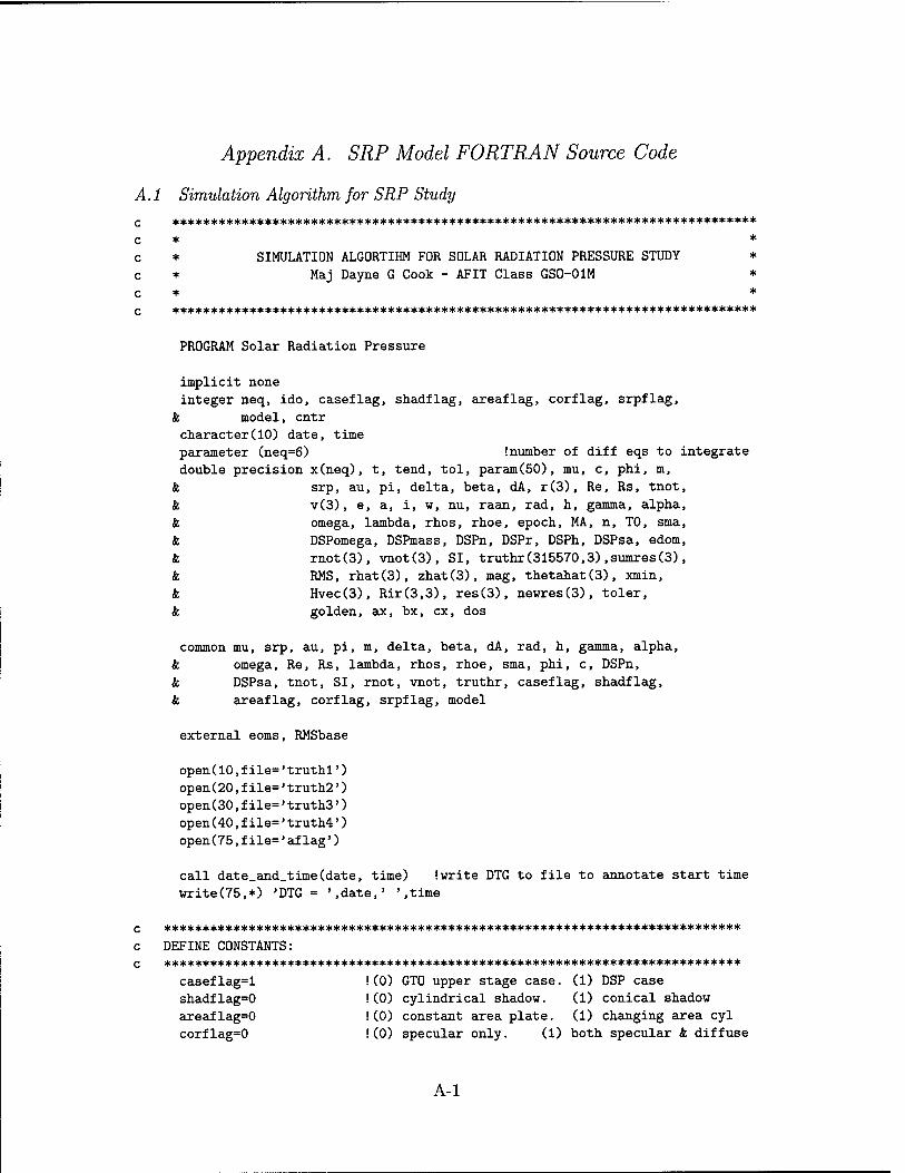
Appendix A. SRP Model FORTRAN Source Code
A.l Simulation Algorithm for SRP Study
c **************************************************************************** c * * c * SIMULATION ALGORTIHM FOR SOLAR RADIATION PRESSURE STUDY *
c * Maj Dayne G Cook - AFIT Class GS0-01M *
c * * c ****************************************************************************
PROGRAM Solar Radiation Pressure
implicit none integer neq, ido, caseflag, shadflag, areaflag, corflag, srpflag,
& model, cntr character(10) date, time parameter (neq=6) !number of diff eqs to integrate
double precision x(neq), t, tend, tol, param(50), mu, c, phi, m,
& srp, au, pi, delta, beta, dA, r(3), Re, Rs, tnot,
& v(3), e, a, i, w, nu, raan, rad, h, gamma, alpha,
& omega, lambda, rhos, rhoe, epoch, MA, n, TO, sma,
& DSPomega, DSPmass, DSPn, DSPr, DSPh, DSPsa, edom,
& mot(3), vnot(3), SI, truthr(315570,3),sumres(3),
& RMS, rhat(3), zhat(3), mag, thetahat(3), xmin,
& Hvec(3), Rir(3,3), res(3), newres(3), toler,
& golden, ax, bx, ex, dos
common mu, srp, au, pi, m, delta, beta, dA, rad, h, gamma, alpha,
& omega, Re, Rs, lambda, rhos, rhoe, sma, phi, c, DSPn,
& DSPsa, tnot, SI, mot, vnot, truthr, caseflag, shadflag,
& areaflag, corflag, srpflag, model
external eoms, RMSbase
open(10,file='truthl')
open(20,file='truth2') open(30,file='truth3')
open(40,file='truth4')
open(75,file='aflag')
call date_and_time(date, time) !write DTG to file to annotate start time
write(75,*) 'DTG = '.date,' '.time
c ***************************************************************************
c DEFINE CONSTANTS: c ***************************************************************************
caseflag=l !(0) GTO upper stage case. (1) DSP case
shadflag=0 !(0) cylindrical shadow. (1) conical shadow areaflag=0 !(0) constant area plate. (1) changing area cyl
corflag=0 !(0) specular only. (1) both specular & diffuse
A-l
srpflag=l
model=0
toler=0.001dO
Re=6378.135d0
Rs=695508d0 pi=dacos(-ldO)
beta=0.75d0
delta=0.5d0 m=14741.752d0
rad=0.001448d0
h=0.005182d0 omega=(pi/4dO)*100dO
DSPomega=(pi/5dO)*100dO
DSPmass=2386dO
DSPn=((2d0*pi)/86145.53)
DSPr=0.00329dO/2dO
DSPh=0.004605dO
DSPsa=5.95d-6 au=149597870.691d0 mu=398600.44180d4
c=299792.458d0
phi=1353d0 sma=l.0000001ldO*au
(0) changing solar flux. (1) constant solar flux
(0) truth model. (1) baseline model
tolerance for golden search algorithm (m)
Radius of the earth (km)
Radius of the sun (km)
define pi=3.14159 fraction of light reflected (coeff of reflection)
fraction of beta specular. (1-delta) is diffuse
satellite mass (kg)
satellite cylindrical radius (km) satellite cylindrical height (km)
spin about bl in 3-21 Euler sequence (rad/100s)
DSP spin rate about b3 (rad/100s)
DSP mass (kg)
*100d0 !DSP mean motion (rad/100s)
!DSP cylinder radius (km)
!DSP cylinder height (km)
!DSP solar array area (km"2)
!1 astronomical unit (km) !gravitational parameter (km~3/100~2s"2)
!speed of light in vacuum (km/s)
!solar radiation flux at sma (W/m"2)
!semi-major axis of earth (km)
if (caseflag==l) then
m=DSPmass
rad=DSPr
h=DSPh
omega=DSPomega
end if
!DSP case
if (corflag==0) then !all specular, no diffuse
delta=ld0
end if
dA=2dO*rad*h ! differential area for baseline (km"2)
c ***************************************************************************
c Given C0ES, convert to r and v c ***************************************************************************
if (caseflag==0) then
a=24509.625d0 e=0.723450073d0
i=25d0*pi/180d0
w=pi raan=pi/2d0
MA=0d0
else if (caseflag==l) then a=42158.135d0
e=0.001d0
i=0.001d0*pi/180d0
w=pi
!typical GT0 orbital elements
!sample DSP orbital elements
A-2
raan=OdO
MA=OdO end if
call COEStoRV(a,e,i,raan,w,MA,rnot,vnot) (Convert COES to r and v
c *********************************************************************
c TRUTH MODEL
c START OF INTEGRATION LOOP FOR EOM'S AND ORBITAL ELEMENTS:
c t and x are both input & output to 'divprk'. 'divprk' stands for double
c precision initial-value problem for ordinary diffeq using Runge-Kutta.
c SET INITIAL CONDITIONS PRIOR TO CALL TO INTEGRATOR:
c t=JD of 1 Jan 2001 in 100 seconds. State vector position x(l-3) is in km. c State vector velocity x(4-6) is in km/100s. tol=iteration tolerance. c ***************************************************************************
tnot=2451910.5d0*864d0 t=tnot
tol=l.d-10 x(l)=rnot(l)
x(2)=rnot(2) x(3)=rnot(3)
x(4)=vnot(l)*100d0
x(5)=vnot(2)*100d0
x(6)=vnot(3)*100d0 cntr=l ido=l !flag indicating state of computation
param(4)=1000000 Isets max # steps allowed
do 100 tend=t,t+315569d0,ld0 Istep size in 100 seconds
call divprk(ido,neq,eoms,t,tend,tol,param,x)
r(l)=x(l) !extract r & v from state x
r(2)=x(2)
r(3)=x(3)
v(l)=x(4)
v(2)=x(5)
v(3)=x(6)
call RVtoC0ES(r,v,a,e,i,raan,w,nu) !input r,v & get COES
c ***************************************************************************
c Write COES and eclipse times to file. c ***************************************************************************
truthr(cntr,:)=r lArchive truth position for future analysis.
cntr=cntr+l
dos=(tend/864d0)-2451910.5d0 !Day of simulation (0-365)
write(20,*) dos.a.e
write(30,*) dos.i.raan
write(40,*) dos.w.nu
if (shadflag==l) then if (lambda <= (rhoe-rhos)) then lumbral
write(10,*) dos, 2d0
A-3
else if (lambda>=(rhoe-rhos) .AND. lambda<=(rhos+rhoe)) then Ipenum
write(10,*) dos, IdO
else write(10,*) dos, OdO !no eclipse
end if
else if (shadflag==0) then
if (SI==0d0) then
write(10,*) dos, IdO
else
write(10,*) dos, OdO
end if
end if
100 continue ido=3 !release workspace
call divprk(ido,neq,eoms,t,tend,tol,param,x) !no integration
c ***************************************************************************
c END OF INTEGRATION LOOP FOR TRUTH MODEL c ***************************************************************************
call date_and_time(date, time) !write DTG to file for computation
write(75,*) 'DTG = '.date,' '.time Itime analysis
write(75,*) 'Truth model run is done.'
close(10, status='save')
close(20, status='save') close(30, status='save')
close(40, status='save')
Q ***************************************************************************
c BASELINE MODEL c ***************************************************************************
model=l !set flag to indicate baseline model
c ax=(dA/4dO) !set bounds on dA for golden section search
C bx=dA
C cx=(2d0*dA)
c RMS=golden(ax,bx,ex,RMSbase,toler,dA)
C write(75,*) 'Minimum RMS in meters is ',RMS
c write(75,*) 'Optimum dA in meters"2 is ',dA*ld6
ax=phi-300d0 !set bounds on phi for golden section search
bx=phi
cx=phi+300d0
RMS=golden(ax,bx,ex,RMSbase,toler,phi)
write(75,*) 'Minimum RMS in meters is ',RMS
write(75,*) 'Optimum phi is ',phi
A-4
call date_and_time(date, time) !write DTG to file for computation
write(75,*) 'DTG = '.date,' '.time Itime analysis
close(75, status='save')
end PROGRAM Solar Radiation Pressure
c *******************************************************************
c END OF MAIN PROGRAM. c ***************************************************************************
c ***************************************************************************
c * *
c * The following routines perform vector manipulation as well as *
c * computation of the classical orbital elements from r and v or *
c * vice versa. * c * * c ***************************************************************************
c ***************************************************************************
c Vector dot product c ***************************************************************************
double precision FUNCTION DOT(V.W) !returns scalar in DOT
implicit none
double precision V(3), W(3)
D0T=V(1)*W(1)+V(2)*W(2)+V(3)*W(3)
return
end
c ***************************************************************************
c Vector cross product c ***************************************************************************
SUBROUTINE CROSS(V.W.Z) !returns vector Z = V cross W
implicit none
double precision V(3), W(3), Z(3)
Z(1)=V(2)*W(3)-W(2)*V(3)
Z(2)=V(3)*W(1)-W(3)*V(1) Z(3)=V(1)*W(2)-W(1)*V(2)
return
end
A-5
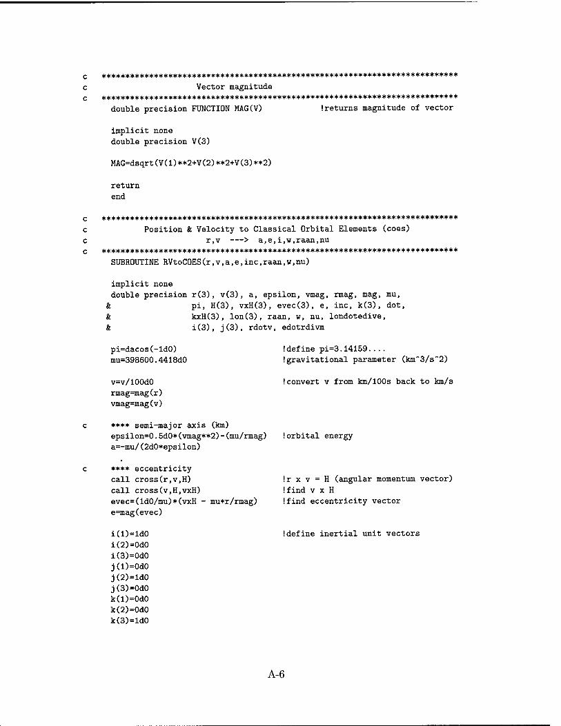
c *************************************************************************** c Vector magnitude c *****************************************************************
double precision FUNCTION MAG(V) !returns magnitude of vector
implicit none
double precision V(3)
MAG=dsqrt(V(l)**2+V(2)**2+V(3)**2)
return
end
c ***************************************************************************
c Position & Velocity to Classical Orbital Elements (coes)
c r,v > a,e,i,w,raan,nu c ***************************************************************************
SUBROUTINE RVtoCOES(r,v,a,e,inc,raan,w,nu)
implicit none double precision r(3), v(3), a, epsilon, vmag, rmag, mag, mu,
& pi, H(3), vxH(3), evec(3), e, inc, k(3), dot,
& kxH(3), lon(3), raan, w, nu, londotedive,
& i(3), j(3), rdotv, edotrdivm
pi=dacos(-ldO)
mu=398600.4418d0
!define pi=3.14159 !gravitational parameter (km~3/s~2)
v=v/100d0 rmag=mag(r)
vmag=mag(v)
!convert v from km/100s back to km/s
**** semi-major axis (km)
epsilon=0.5d0*(vmag**2)-(mu/rmag)
a=-mu/(2d0*epsilon)
!orbital energy
**** eccentricity
call cross(r,v,H)
call cross(v,H,vxH)
evec=(ldO/mu)*(vxH -
e=mag(evec)
mu*r/rmag)
!r x v = H (angular momentum vector)
!find v x H Ifind eccentricity vector
i(l)=ldO
i(2)=0d0
i(3)=0d0
j(l)=0d0
j(2)=ld0
j(3)=0d0 k(l)=OdO
k(2)=0d0 k(3)=ld0
!define inertial unit vectors
A-6
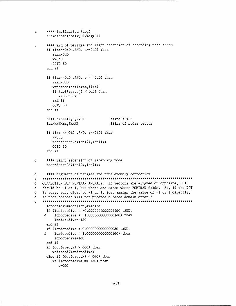
c HC*** inclination (deg)
inc=dacosd(dot(k,H)/mag(H))
c **** arg of perigee and right ascension of ascending node cases
if (inc==0d0 .AND. e==0d0) then
raan=0d0
w=0d0
GOTO 50 end if
if (inc==0d0 .AND. e <> OdO) then
raan=0d0 w=dacosd(dot(evec,i)/e)
if (dot(evec,j) < OdO) then
w=360d0-w
end if
GOTO 50
end if
call cross(k.H.kxH) !find k x H lon=kxH/mag(kxH) lline of nodes vector
if (inc <> OdO .AND. e==0d0) then
w=0d0
raan=datan2d(lon(2),lon(l))
GOTO 50 end if
c **** right ascension of ascending node
raan=datan2d(lon(2) ,lon(D)
c **** argument of perigee and true anomaly correction c ***************************************************************************
c CORRECTION FOR FORTRAN ANOMALY: If vectors are aligned or opposite, DOT c should be -1 or 1, but there are cases where FORTRAN folds. So, if the DOT
c is very, very close to -1 or 1, just assign the value of -1 or 1 directly,
c so that 'dacos' will not produce a 'acos domain error.' c ***************************************************************************
londotedive=dot(Ion,evec)/e
if (londotedive < -0.99999999999999d0 .AND. & londotedive > -l.OOOOOOOOOOOOOldO) then
londotedive=-ldO
end if
if (londotedive > 0.99999999999999d0 .AND.
& londotedive < l.OOOOOOOOOOOOOldO) then
londotedive=ldO
end if
if (dot(evec,k) > OdO) then w=dacosd(londotedive)
else if (dot(evec,k) < OdO) then if (londotedive == IdO) then
w=0d0
A-7
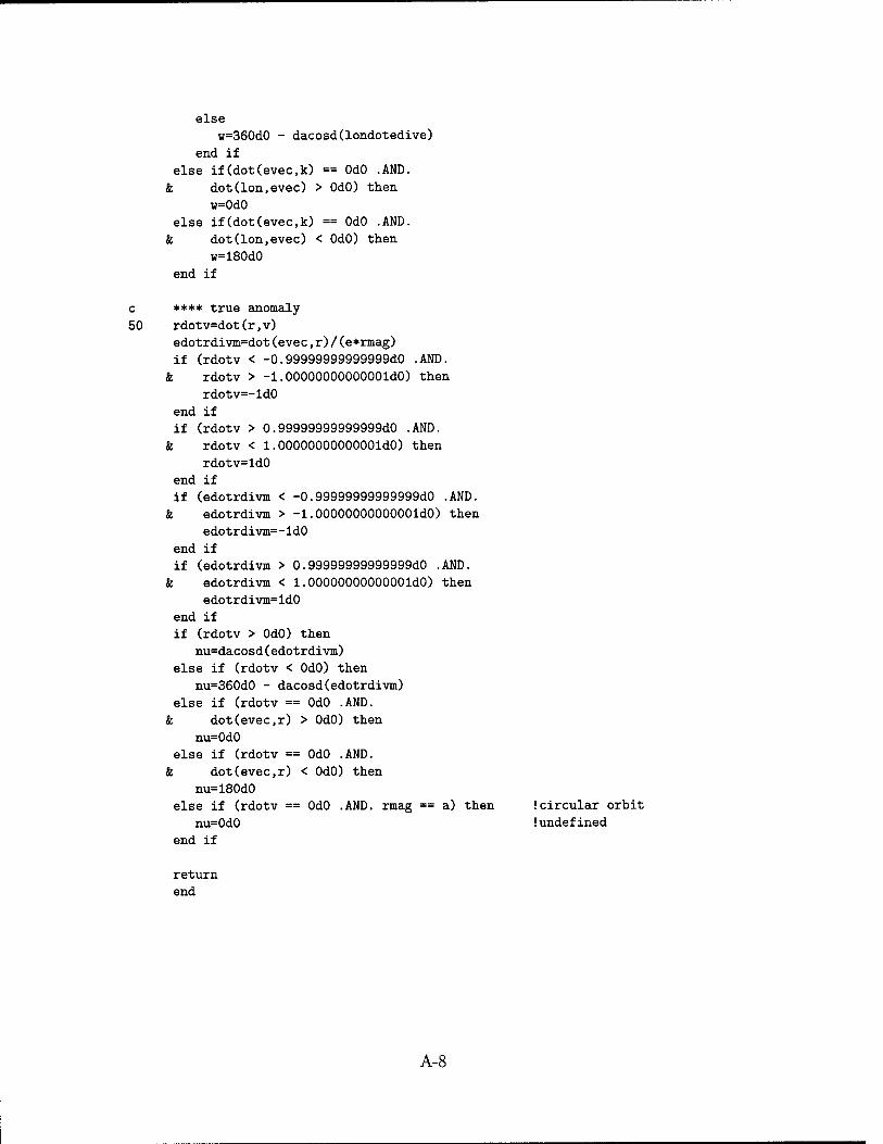
else w=360d0 - dacosd(londotedive)
end if
else if(dot(evec,k) == OdO .AND.
& dot(Ion,evec) > OdO) then
w=0d0 else if(dot(evec,k) == OdO .AND.
& dot(Ion,evec) < OdO) then
w=180d0
end if
c **** true anomaly
50 rdotv=dot(r,v) edotrdivm=dot(evec,r)/(e*rmag)
if (rdotv < -0.99999999999999d0 .AND.
& rdotv > -l.OOOOOOOOOOOOOldO) then
rdotv=-ld0
end if if (rdotv > 0.99999999999999d0 .AND.
& rdotv < l.OOOOOOOOOOOOOldO) then
rdotv=ld0 end if if (edotrdivm < -0.99999999999999d0 .AND.
& edotrdivm > -l.OOOOOOOOOOOOOldO) then
edotrdivm=-IdO
end if if (edotrdivm > 0.99999999999999d0 .AND.
& edotrdivm < l.OOOOOOOOOOOOOldO) then
edotrdivm=ldO
end if
if (rdotv > OdO) then nu=dacosd(edotrdivm)
else if (rdotv < OdO) then
nu=360d0 - dacosd(edotrdivm)
else if (rdotv == OdO .AND.
& dot(evec,r) > OdO) then
nu=0d0 else if (rdotv == OdO .AND.
& dot(evec,r) < OdO) then
nu=180d0 else if (rdotv == OdO .AND. rmag == a) then !circular orbit
nu=0d0 (undefined
end if
return
end
A-8
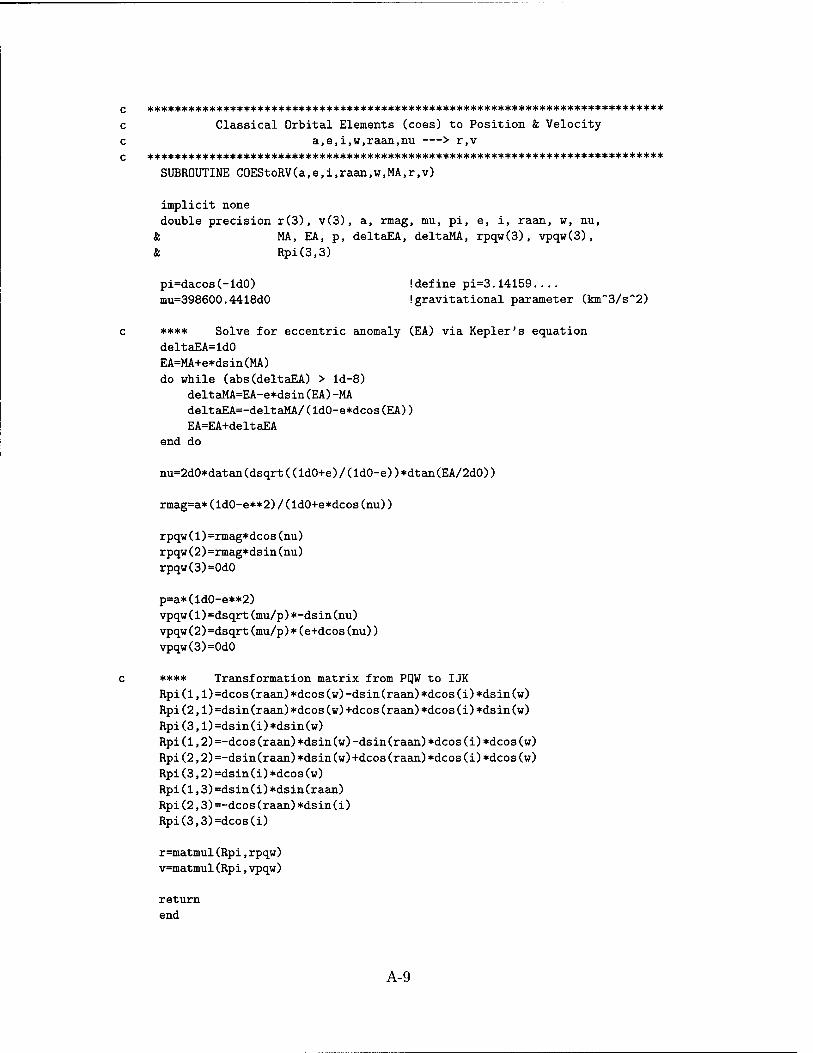
c **************************************************************************
c Classical Orbital Elements (coes) to Position & Velocity
c a,e,i,w,raan,nu > r,v c ***************************************************************************
SUBROUTINE COEStoRV(a,e,i,raan,w,MA,r,v)
implicit none double precision r(3), v(3), a, rmag, mu, pi, e, i, raan, w, nu,
& MA, EA, p, deltaEA, deltaMA, rpqw(3), vpqw(3),
& Rpi(3,3)
pi=dacos(-ldO) Idefine pi=3.14159
mu=398600.4418d0 !gravitational parameter (km~3/s~2)
c **** Solve for eccentric anomaly (EA) via Kepler's equation
deltaEA=ldO
EA=MA+e*dsin(MA)
do while (abs(deltaEA) > ld-8) deltaMA=EA-e*dsin(EA)-MA
deltaEA=-deltaMA/(ldO-e*dcos(EA)) EA=EA+deltaEA
end do
nu=2d0*datan(dsqrt((IdO+e)/(IdO-e))*dtan(EA/2dO))
rmag=a*(ld0-e**2)/(ldO+e*dcos(nu))
rpqw(1)=rmag*dcos(nu)
rpqw(2)=rmag*dsin(nu)
rpqw(3)=0d0
p=a*(ld0-e**2) vpqw(l)=dsqrt(mu/p)*-dsin(nu)
vpqw(2)=dsqrt(mu/p)*(e+dcos(nu))
vpqw(3)=0d0
c **** Transformation matrix from PQW to IJK
Rpi(l,l)=dcos(raan)*dcos(w)-dsin(raan)*dcos(i)*dsin(w)
Rpi(2,1)=dsin(raan)*dcos(w)+dcos(raan)*dcos(i)*dsin(w)
Rpi(3,l)=dsin(i)*dsin(w)
Rpi(1,2)=-dcos(raan)*dsin(w)-dsin(raan)*dcos(i)*dcos(w)
Rpi(2,2)=-dsin(raan)*dsin(w)+dcos(raan)*dcos(i)*dcos(w)
Rpi(3,2)=dsin(i)*dcos(w)
Rpi(l,3)=dsin(i)*dsin(raan)
Rpi(2,3)=-dcos(raan)*dsin(i) Rpi(3,3)=dcos(i)
r=matmul(Rpi,rpqw) v=matmul(Rpi,vpqw)
return end
A-9
*************************************************************************** * * * EQUATIONS OF MOTION (EOMS) SUBROUTINE * * * ****************************************************************************
SUBROUTINE eoms(neq,t,x,xdot) Ixdot is the output
implicit none integer neq, cntr, caseflag, shadflag, areaflag, corflag, srpflag,
i model double precision t, x(neq), xdot(neq), au, mu, srp, sun(6), r(3),
k s(3), svsun(3), mag, dA, dot, Re, Rs, nhat(3), tnot, k svsunhat(3), pi, m, theta, beta, delta, ndotsv, rad, h, sma, k Rbi(3,3), Rib(3,3), gamma, alpha, omega, svsunhatb(3), bl(3), k b2(3), b3(3), Ab(3), Ai(3), svsunhatbpj(3), psi, cylends(3), fc rhos, rhoe, SI, lambda, A, U, Q, cosPsi, v(3), Hvec(3), i(3), fc j(3), bli(3), bliproj(3), phi, c, DSPn, DSPsa, nlhat(3), k n2hat(3), n3hat(3), n4hat(3), SP1(3), SP2(3), SP3(3), SP4(3), it b3i(3), b3check(3), truthr(315570,3), rnot(3), vnot(3)
common mu, srp, au, pi, m, delta, beta, dA, rad, h, gamma, alpha, It omega, Re, Rs, lambda, rhos, rhoe, sma, phi, c, DSPn, k DSPsa, tnot, SI, mot, vnot, truthr, caseflag, shadflag, k areaflag, corflag, srpflag, model
c ***************************************************************************
c EXTRACT SUN VECTOR FROM EPHEMERIS FILE: c 'pleph'(located in 'ephem.f') returns sun vector (r & v) in AU wrt earth, c Define Sat & Sun vectors(ECI). SRP constant is a function of (sma/|s|)"2. c ***************************************************************************
call pleph(t/864d0,11,3,sun) !864 by 100s per block per day
do cntr=l,3 r(cntr)=x(cntr) v(cntr)=x(cntr+3) s(cntr)=sun(cntr)*au
end do
!r = earth to SV !v = sat velocity vector !s = earth to sun (convert to km)
svsun=s-r svsunhat=svsun/mag(svsun)
(define vector SV to sun (ECI) limit vector from SV to sun (ECI)
srp=(phi*(sma/mag(s))**2/c)*100d2 if (model==0 .AND. srpflag==l) then
srp=(phi/c)*100d2 end if
!SRP constant (N/10~7m~2)
!SRP constant (N/10Tm~2)
if (model==0 .AND. shadflag==l) then
A-10
c ***************************************************************************
c CONICAL SHADOW MODEL: c Determine whether SV is in penumbra, umbra, or no eclipse. Additionally,
c find the fraction of solar intensity (SI) in each case.
c Umbra(SI=0) , no eclipse (SI=1) , penumbra(0<SKl) . c ***************************************************************************
lambda=dacos(dot(svsunhat,-r)/mag(r)) !earth-SV-sun angle
rhos=dasin(Rs/mag(svsun)) !sun angular radius from SV rhoe=dasin(Re/mag(r)) !earth angular radius from SV
if (lambda >= (rhos+rhoe)) then !no eclipse
SI=ldO
else if (lambda <= (rhoe-rhos)) then lumbral
SI=0d0 else Ipenumbral
Q=0.5d0*(rhos+rhoe+lambda) U=(2d0/lambda)*dsqrt(Q*(Q-lambda)*(Q-rhos)*(Q-rhoe))
if (abs(rhos**2-rhoe**2) <= lambda**2) then A=(dasin(U/rhos))*rhos**2+(dasin(U/rhoe))*rhoe**2-U*lambda
else if (abs(rhos**2-rhoe**2) > lambda**2) then A=rhoe**2*dasin(U/rhoe)+(pi-dasin(U/rhos))*rhos**2-U*lambda
end if
SI=ldO - A/(pi*rhos**2)
end if
else
c ***************************************************************************
c SIMPLIFIED CYLINDRICAL SHADOW MODEL: c For the baseline model, determine if SV is in cylindrical earth shadow or
c not. In shadow (SI=0), outside of shadow (SI=1). c ***************************************************************************
cosPsi=dot(r,s)/(mag(r)*mag(s)) if (cosPsi<0d0 .AND. (mag(r)**2-mag(r)**2*cosPsi**2)<Re**2) then
SI=0d0 else
SI=ldO
end if end if lend of shadow flag check
c ***************************************************************************
C DEFINE INERTIAL AND BODY FRAME UNIT VECTORS: c ***************************************************************************
i(l)=ldO
i(2)=0d0
i(3)=0d0
j(l)=0d0
j(2)=ld0
j(3)=0d0 bl(l)=ldO
bl(2)=0d0 bl(3)=0d0
b2(l)=0d0
A-ll
b2(2)=ld0
b2(3)=0d0
b3(l)=0d0
b3(2)=0d0
b3(3)=ld0
if (model==l) then
GOTO 500
end if if (areaflag==0) then
GOTO 400
end if
c *****************************************************************
c EULER ROTATION ANGLES:
c For the case of a prolate, cylindrical spent upper stage; the body will
c degenerate to spinning about its' max MOI with spin axis normal to the
c orbital plane as equilibrium. Case of a torque-free axisymmetric rigid body. c ***************************************************************************
if (caseflag==0) then
call cross(r,v,Hvec)
bli=Hvec/mag(Hvec)
bliproj(l)=bli(l)
bliproj(2)=bli(2)
bliproj(3)=0d0
gamma=dasin(bli(3)) alpha=dacos(dot(i.bliproj)/mag(bliproj)) if (dot(j,bliproj) < OdO) then Iquadrant correction: alpha > 180
alpha=2d0*pi-alpha else if (bli(3) == IdO) then !bl is along k
alpha=0d0 end if
end if
c ***************************************************************************
c DEFINE TRANSFORMATION MATRIX: c (0) US cylindrical body — Inertial to {b} via a (3, -2, 1) Euler rotation.
c (1) DSP case — Inertial to {b} via a (3, -2, 3) Euler rotation. c ***************************************************************************
if (caseflag==0) then !GT0 upper stage case
Rib(1,1)=dcos(gamma)*dcos(alpha) Rib(2,l)=-dcos(omega*t)*dsin(alpha)-
& dsin(omega*t)*dsin(gamma)*dcos(alpha)
Rib(3,l)=dsin(omega*t)*dsin(alpha)- & dcos(omega*t)*dsin(gamma)*dcos(alpha)
Rib(1,2)=dcos(gamma)*dsin(alpha)
Rib(2,2)=dcos(omega*t)*dcos(alpha)- & dsin(omega*t)*dsin(gamma)*dsin(alpha)
Rib(3,2)=-dsin(omega*t)*dcos(alpha)- & dcos(omega*t)*dsin(gamma)*dsin(alpha)
Rib(1,3)=dsin(gamma)
A-12
Rib(2,3)=dsin(omega*t)*dcos(gamma)
Rib(3,3)=dcos(omega*t)*dcos(gamma)
else if (caseflag==l) then !DSP case Rib(l,l)=-dsin(omega*(t-tnot))*dsin(DSPn*(t-tnot))
Rib(2,1)=-dcos(omega*(t-tnot))*dsin(DSPn*(t-tnot))
Rib(3,l)=-dcos(DSPn*(t-tnot))
Rib(1,2)=dsin(omega*(t-tnot))*dcos(DSPn*(t-tnot))
Rib(2,2)=dcos(omega*(t-tnot))*dcos(DSPn*(t-tnot)) Rib(3,2)=-dsin(DSPn*(t-tnot))
Rib(1,3)=dcos(omega*(t-tnot))
Rib(2,3)=-dsin(omega*(t-tnot))
Rib(3,3)=0d0
end if
c ************************************************
c TRANSPOSE: Get sv-sun unit vector in {b} components and then calculate the
c angle between its' projection and bl in the bl-b2 plane. c ***************************************************************************
Rbi=transpose(Rib) svsunhatb=matmul(Rib,svsunhat) !transform svsunhat from ECI to [b]
svsunhatbpj(l)=svsunhatb(l) (project svsunhatb into bl-b2 plane
svsunhatbpj(2)=svsunhatb(2)
svsunhatbpj(3)=0d0
psi=dacos(dot(bl,svsunhatbpj)/mag(svsunhatbpj))
if (dot(b2,svsunhatbpj) < OdO) then !quadrant correction
psi=2d0*pi-psi
end if
c ***************************************************************************
c Calculate SRP component acceleration contribution of cylinder ends in {b}.
c dot(svsunhat,b3) determines angle between sv-sun vector and b3 or normal, c ***************************************************************************
if (dot(svsunhatb,b3) > OdO) then !top of cylinder illuminated
nhat=b3 else
nhat=-b3 end if cylends=-(2d0*delta*beta*(srp/m)*dot(svsunhatb,nhat)**2*pi*
& rad**2 + (Id0-delta)*beta*(2d0/3d0)*(srp/m)*pi*rad**2*
& dot(svsunhatb,nhat))*nhat - ((ldO-delta*beta)*(srp/m)*
& dot(svsunhatb,nhat)*pi*rad**2)*svsunhatb
c ***************************************************************************
c Calculate SRP component acceleration contribution of the 4 solar array
c panels on DSP in {b}. c ***************************************************************************
if (caseflag==0) then !If GTO upper stage case, then pad with do cntr=l,3 !zeros and skip over panels section to 300
SPl(cntr)=0d0 SP2(cntr)=0d0
SP3(cntr)=0d0
A-13
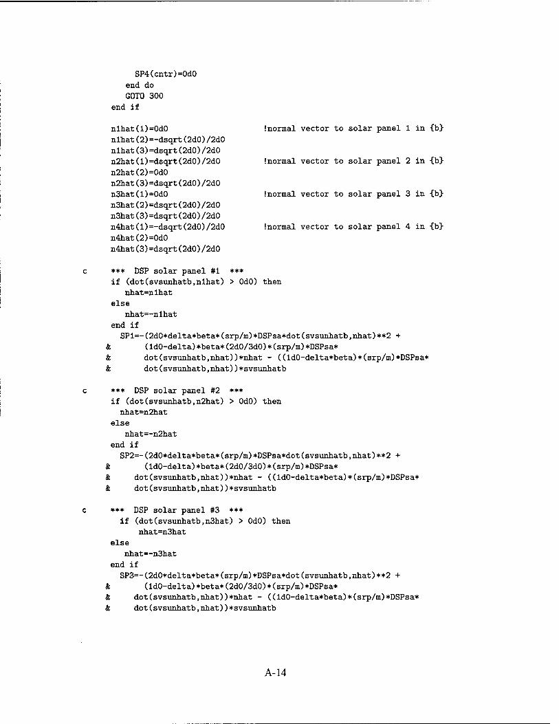
SP4(cntr)=0d0 end do GOTO 300
end if
nlhat(l)= nlhat(2)= nlhat(3)= n2hat(l)= n2hat(2)= n2hat(3)= n3hat(l)= n3hat(2)= n3hat(3)= n4hat(l)= n4hat(2)= n4hat(3)=
=0d0 =-dsqrt(2d0)/2d0 =dsqrt(2d0)/2d0 =dsqrt(2d0)/2d0 'OdO >dsqrt(2d0)/2d0 <0d0 >dsqrt(2d0)/2d0 <dsqrt(2d0)/2d0 >-dsqrt(2d0)/2d0 tfdO <dsqrt(2d0)/2d0
!normal vector to solar panel 1 in {b}
!normal vector to solar panel 2 in {b}
!normal vector to solar panel 3 in {b}
!normal vector to solar panel 4 in {b}
*** DSP solar panel #1 *** if (dot(svsunhatb,nlhat) > OdO) then
nhat=nlhat else
nhat=-nlhat end if SP1=-(2d0*delta*beta*(srp/m)*DSPsa*dot(svsunhatb,nhat)**2 +
fe (IdO-delta)*beta*(2d0/3d0)*(srp/m)*DSPsa* fe dot(svsunhatb,nhat))*nhat - ((ldO-delta*beta)*(srp/m)*DSPsa* fe dot(svsunhatb,nhat))*svsunhatb
*** DSP solar panel #2 *** if (dot(svsunhatb,n2hat) > OdO) then nhat=n2hat
else nhat=-n2hat
end if SP2=-(2d0*delta*beta*(srp/m)*DSPsa*dot(svsunhatb,nhat)**2 +
fc (IdO-delta) *beta* (2d0/3d0) * (srp/m) *DSPsa* I dot(svsunhatb,nhat))*nhat - ((ldO-delta*beta)*(srp/m)*DSPsa* i dot(svsunhatb,nhat))*svsunhatb
*** DSP solar panel #3 *** if (dot(svsunhatb,n3hat) > OdO) then
nhat=n3hat else
nhat=-n3hat end if SP3=-(2dO*delta*beta*(srp/m)*DSPsa*dot(svsunhatb,nhat)**2 +
it (IdO-delta) *beta* (2d0/3d0) * (srp/m) *DSPsa* k dot(svsunhatb,nhat))*nhat - ((ldO-delta*beta)*(srp/m)*DSPsa* i, dot(svsunhatb,nhat))*svsunhatb
A-14
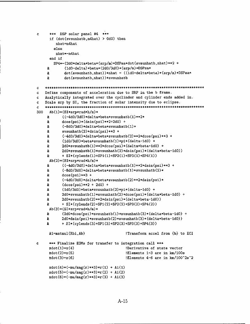
c *** DSP solar panel #4 ***
if (dot(svsunhatb,n4hat) > OdO) then
nhat=n4hat
else
nhat=-n4hat
end if SP4=-(2d0*delta*beta*(srp/m)*DSPsa*dot(svsunhatb,nhat)**2 +
& (IdO-delta)*beta*(2d0/3d0)*(srp/m)*DSPsa* & dot(svsunhatb,nhat))*nhat - ((ldO-delta*beta)*(srp/m)*DSPsa*
& dot(svsunhatb,nhat))*svsunhatb
c *****************************************************************
c Define components of acceleration due to SRP in the b frame.
c Analytically integrated over the cyclinder and cylinder ends added in.
c Scale srp by SI, the fraction of solar intensity due to eclipse. c ***************************************************************************
300 Ab(l)=(SI*srp*rad*h/m)* & ((-4d0/3d0)*delta*beta*svsunhatb(l)**2*
& dcos(psi)*(dsin(psi)**2+2d0) + & (-8d0/3d0)*delta*beta*svsunhatb(l)*
& svsunhatb(2)*dsin(psi)**3 + & (-4d0/3d0)*delta*beta*svsunhatb(2)**2*dcos(psi)**3 +
& (Id0/3d0)*beta*svsunhatb(l)*pi*(delta-ld0) +
& 2d0*svsunhatb(l)**2*dcos(psi)*(delta*beta-ld0) +
& 2d0*svsunhatb(l)*svsunhatb(2)*dsin(psi)*(delta*beta-ld0))
& + SI*(cylends(l)+SPl(l)+SP2(l)+SP3(l)+SP4(D)
Ab(2)=(SI*srp*rad*h/m)* & ((-4d0/3d0)*delta*beta*svsunhatb(l)**2*dsin(psi)**3 +
& (-8d0/3d0)*delta*beta*svsunhatb(l)»svsunhatb(2)*
& dcos(psi)**3 + & (-4d0/3d0)*delta*beta*svsunhatb(2)**2*dsin(psi)*
& (dcos(psi)**2 + 2d0) +
& (Id0/3d0)*beta*svsunhatb(2)*pi*(delta-ld0) +
& 2d0*svsunhatb(l)*svsunhatb(2)*dcos(psi)*(delta*beta-ld0) +
& 2d0*svsunhatb(2)**2*dsin(psi)*(delta*beta-ldO)) & + SI*(cylends(2)+SPl(2)+SP2(2)+SP3(2)+SP4(2))
Ab(3)=(SI*srp*rad*h/m)* & (2d0*dcos(psi)*svsunhatb(l)*svsunhatb(3)*(delta*beta-ld0) +
& 2d0*dsin(psi)*svsunhatb(2)*svsunhatb(3)*(delta*beta-ld0))
& + SI*(cylends(3)+SPl(3)+SP2(3)+SP3(3)+SP4(3))
Ai=matmul(Rbi,Ab) !Transform accel from {b} to ECI
c *** Finalize EOMs for transfer to integration call ***
Xdot(l)=x(4) !Derivative of state vector
xdot(2)=x(5) lElements 1-3 are in km/100s
xdot(3)=x(6) lElements 4-6 are in km/100"2s"2
xdot(4)=(-mu/mag(r)**3)*r(l) + Ai(l)
xdot(5)=(-mu/mag(r)**3)*r(2) + Ai(2) xdot(6)=(-mu/mag(r)**3)*r(3) + Ai(3)
A-15
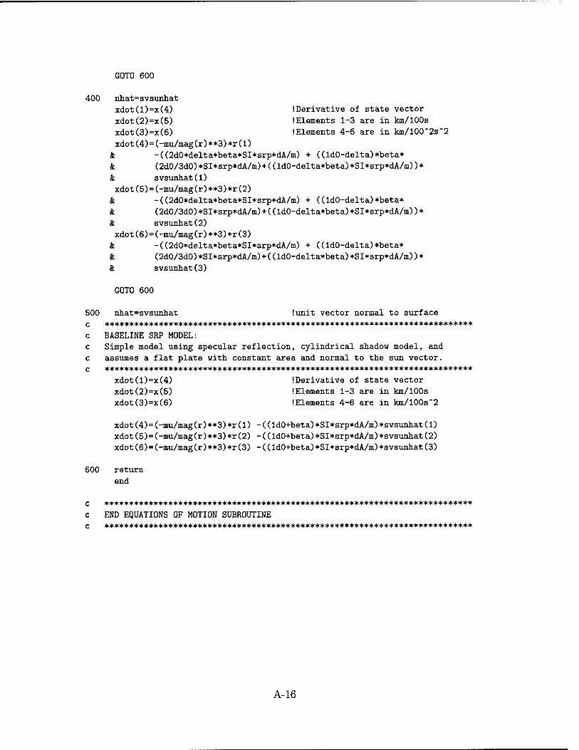
GOTO 600
400 nhat=svsunhat xdot(l)=x(4) IDerivative of state vector
xdot(2)=x(5) !Elements 1-3 are in km/100s
xdot(3)=x(6) (Elements 4-6 are in km/100"2s~2
xdot(4)=(-mu/mag(r)**3)*r(l) & -((2d0*delta*beta*SI*srp*dA/m) + ((ldO-delta)*beta* & (2d0/3d0)*SI*srp*dA/m)+((ld0-delta*beta)*SI*srp*dA/m))*
& svsunhat(1)
xdot(5)=(-mu/mag(r)**3)*r(2)
& -((2dO*delta*beta*SI*srp*dA/m) + ((ld0-delta)*beta*
& (2d0/3d0)*SI*srp*dA/m)+((ldO-delta*beta)*SI*srp*dA/m))*
& svsunhat(2)
xdot(6)=(-mu/mag(r)**3)*r(3)
& -((2dO*delta*beta*SI*srp*dA/m) + ((ldO-delta)*beta* & (2d0/3d0)*SI*srp*dA/m)+((ldO-delta*beta)*SI*srp*dA/m))*
& svsunhat(3)
GOTO 600
500 nhat=svsunhat lunit vector normal to surface c ****************************************************************
c BASELINE SRP MODEL: c Simple model using specular reflection, cylindrical shadow model, and
c assumes a flat plate with constant area and normal to the sun vector. c ***************************************************************************
xdot(l)=x(4) IDerivative of state vector
xdot(2)=x(5) lElements 1-3 are in km/100s xdot(3)=x(6) lElements 4-6 are in km/100s~2
xdot(4)=(-mu/mag(r)**3)*r(1) -((IdO+beta)*SI*srp*dA/m)*svsunhat(1) xdot(5)=(-mu/mag(r)**3)*r(2) -((ld0+beta)*SI*srp*dA/m)*svsunhat(2)
xdot(6)=(-mu/mag(r)**3)*r(3) -((IdO+beta)*SI*srp*dA/m)*svsunhat(3)
600 return
end
c ***************************************************************************
c END EQUATIONS OF MOTION SUBROUTINE c ***************************************************************************
A-16
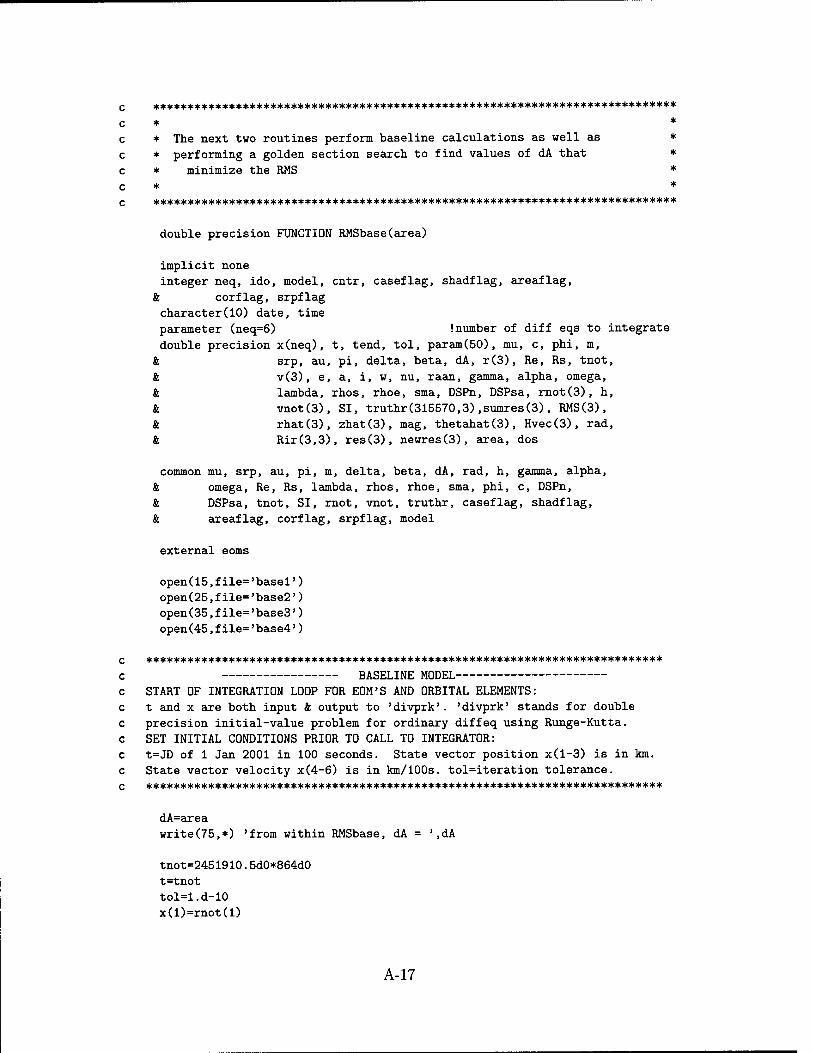
c *************************************************************************
c * * c * The next two routines perform baseline calculations as well as * c * performing a golden section search to find values of dA that * c * minimize the RMS * c * *
c ****************************************************************************
double precision FUNCTION RMSbase(area)
implicit none integer neq, ido, model, cntr, caseflag, shadflag, areaflag,
& corflag, srpflag character(10) date, time parameter (neq=6) !number of diff eqs to integrate double precision x(neq), t, tend, tol, param(50), mu, c, phi, m,
k srp, au, pi, delta, beta, dA, r(3), Re, Rs, tnot, k v(3), e, a, i, w, nu, raan, gamma, alpha, omega, k lambda, rhos, rhoe, sma, DSPn, DSPsa, rnot(3), h, k vnot(3), SI, truthr(315570,3),sumres(3), RMS(3), k rhat(3), zhat(3), mag, thetahat(3), Hvec(3), rad, & Rir(3,3), res(3), newres(3), area, dos
common mu, srp, au, pi, m, delta, beta, dA, rad, h, gamma, alpha, k omega, Re, Rs, lambda, rhos, rhoe, sma, phi, c, DSPn, k DSPsa, tnot, SI, mot, vnot, truthr, caseflag, shadflag, k areaflag, corflag, srpflag, model
external eoms
open(15,file='basel') open(25,file='base2') open(35,file='base3') open(45,file=,base4')
c ***************************************************************************
c BASELINE MODEL c START OF INTEGRATION LOOP FOR EOM'S AND ORBITAL ELEMENTS: c t and x are both input k output to 'divprk'. 'divprk' stands for double c precision initial-value problem for ordinary diffeq using Runge-Kutta. C SET INITIAL CONDITIONS PRIOR TO CALL TO INTEGRATOR: c t=JD of 1 Jan 2001 in 100 seconds. State vector position x(l-3) is in km. c State vector velocity x(4-6) is in km/100s. tol=iteration tolerance. c ***************************************************************************
dA=area write(75,*) 'from within RMSbase, dA = ' ,dA
tnot=2451910.5d0*864d0 t=tnot tol=l.d-10 x(l)=rnot(l)
A-17
x(2)=rnot(2)
x(3)=rnot(3) x(4)=vnot(l)*100d0
x(5)=vnot(2)*100d0 x(6)=vnot(3)*100d0
cntr=l
sumres=OdO ido=l !ido = flag indicating state of computation
param(4)=1000000 Isets max # steps allowed
do 200 tend=t,t+315569d0,ld0 Istep size in 100 seconds call divprk(ido,neq,eoms,t,tend,tol,param,x)
r(l)=x(l) (extract r & v from state x
r(2)=x(2)
r(3)=x(3)
v(l)=x(4)
v(2)=x(5)
v(3)=x(6)
call RVtoC0ES(r,v,a,e,i,raan,w,nu) !input r,v & get C0ES
c call E0V(t, w, raan, edom)
c **********************************************************************
c Write C0ES and eclipse times to file. c ***************************************************************************
dos=(tend/864d0)-2451910.5d0 !day of simulation
write(25,*) dos.a.e
write(35,*) dos,i,raan
write(45,*) dos.w.nu
if (SI==0d0) then write(15,*) tend, IdO
else
write(15,*) tend, OdO
end if
c ***************************************************************************
c Compute transformation ijk to ric. Transform/sum residuals in new frame, c ***************************************************************************
rhat=r/mag(r) call cross(r,v,Hvec)
zhat=Hvec/mag(Hvec)
call cross(zhat.rhat.thetahat)
Rir(l,:)=rhat
Rir(2,:)=thetahat
Rir(3,:)=zhat
res=r-truthr(cntr,:)
newres=matmul(Rir,res) sumres=sumres+newres**2
cntr=cntr+l
A-18
200 continue
ido=3 call divprk(ido,neq,eoms,t,tend,tol,param,x)
close(15, status='save') close(25, status='save') close(35, status='save') close(45, status='save')
RMS=dsqrt(sumres/315570d0)*ld3
RMSbase=mag(RMS)
write(75,*) 'RMSr(m) = \RMS(1)
write(75,*) 'RMSi(m) = ',RMS(2) write(75,*) 'RMSc(m) = ',RMS(3)
write(75,*) 'mag RMS(m) = '.RMSbase
call date_and_time(date, time)
write(75,*) 'DTG = '.date,' '.time
return
end
!release workspace
!no integration
[convert km to m
c ***************************************************************************
c Golden Section Search Algorithm c *********************************************************
double precision FUNCTION golden(ax,bx,ex,RMSbase,toler,phi)
implicit none
double precision ax, bx, ex, toler, dA, RMSbase, beta, & fl, f2, xO, xl, x2, x3, R, C, phi, Re
external RMSbase
parameter(R=0.61803399d0, C=ld0-R)
c ***************************************************************************
c Given a function (RMSbase), and given a bracketing triplet of abscissas
c ax, bx, ex (such that bx is between ax and ex, and f(bx) is less than c f(ax) and f(cx)), this routine performs a golden section search for the
c minimum, isolating it to a fractional precision of about toler. The
c abscissa of the minimum is returned as xmin, and the minimum function
c value is returned as golden. Parameters: The golden ratios. c ***************************************************************************
x0=ax !at any given time, keep track of 4 points;x0,xl,x2,x3
x3=cx if (abs(cx-bx) > abs(bx-ax)) then Imake xO to xl the smaller segment
xl=bx x2=bx+C*(cx-bx) !& fill in the new point to be tried,
else
A-19
x2=bx
xl=bx-C*(bx-ax)
end if
fl=RMSbase(xl) !initial function evaluations, note that we never
f2=RMSbase(x2) !need to evaluate the function at original endpoints.
if (abs(fl-f2) > toler) then
write(*,*) >abs(fl-f2) = >,abs(fl-f2)
write(75,*) Jabs(fl-f2) = ',abs(fl-f2)
if (f2 < fl) then lone possible outcome xO=xl !its housekeeping
xl=x2
x2=R*xl+C*x3
fl=f2 f2=RMSbase(x2) land a new function evaluation
else I the other outcome
x3=x2
x2=xl
xl=R*x2+C*xO f2=fl fl=RMSbase(xl) land its new funstion evaluation
end if goto 1 Iback to see if we're done
end if
if (fl < f2) then I done, output best of current values
golden=f1
dA=xl
else
golden=f2
dA=x2
end if
return end
A-20
A.2 JPL Planetary and Lunar Ephemerides
Q *************************************************************************** C * * C * JPL Planetary and Lunar Ephemerides * C * * Q ***************************************************************************
C C Version : July 8, 1997 C C Program TESTEPH {First part of main program has been deleted so C as not to conflict with main of SRP.f. See original C file, testeph.f for complete testing code — Dayne Cook} C C TESTEPH tests the JPL ephemeris reading and interpolating routine using C examples computed from the original ephemeris. C C TESTEPH contains the reading and interpolating subroutines that are of C eventual interest to the user. Once TESTEPH is working correctly, the C user can extract those subroutines and the installation process is complete. C C You must supply "testpo.XXX" to TESTEPH, via standard input. "testpo.XXX C is the specially formatted text file that contains the test cases for the C ephmeris, DEXXX. C C After the initial identifying text which is concluded by an "EOT" in C columns 1-3, the test file contains the following quantities: C C JPL Ephemeris Number C calendar date C Julian Ephemeris Date C target number (1-Mercury, ...,3-Earth, ,,,9-Pluto, 10-Moon, 11-Sun, C 12-Solar System Barycenter, 13-Earth-Moon Barycenter C 14-Nutations, 15-Librations) C center number (same codes as target number) C coordinate number (1-x, 2-y, ... 6-zdot) C coordinate [au, au/day] C C For each test case input, TESTEPH C C - computes the corresponding state from data contained C in DExxx, C C - compares the two sets, C C - writes an error message if the difference between C any of the state components is greater than 10**(-13). C C - writes state and difference information for every 10th C test case processed. C C C This program is written in standard Fortran-77.
A-21
HOWEVER, there are two parts which are compiler dependent; both have
to do with opening and reading a direct-access file. They are dealt
with in the subroutine FSIZERi, i=l,3. (There are three versions of
this subroutine.
1) The parameter RECL in the OPEN statement is the number of units per
record. For some compilers, it is given in bytes; in some, it is given
in single precision words. In the subroutine FSIZER of TESTEPH, the
parameter NRECL must be set to 4 if RECL is given in bytes; NRECL must
be set to 1 if RECL is given in words. (If in doubt, use 4 for UNIX;
1 for VAX and PC)
2) Also for the OPEN statement, the program needs to know the exact value
of RECL (number of single precision words times NRECL). Since this
varies from one JPL ephemeris to another, RECL must be determined somehow
and given to the OPEN statement. There are three methods, depending
upon the compiler. We have included three versions of the subroutine
FSIZER, one for each method.
a) Use the INQUIRE statement to find the length of the records automatically before opening the file. This works for VAX's;
not in UNIX.
b) Open the file with an arbitrary value of RECL, read the first record,
and use the information on that record to determine the exact value
of RECL. Then, close the file and re-open it with the exact value.
This seems to work for UNIX compilers as long as the initial value of
RECL is less than the exact value but large enough to get the required
information from the first file. (For other compilers, this doesn't
work since you can open a file only with the exact value of RECL.)
c) Hardwire the value of RECL. This number is NRECL*1652 for DE200,
NRECL*2036 for DE405, and NRECL*1456 for DE406.
C C Version 1.0 uses the INQUIRE statement to find out the the record length
C of the direct access file before opening it. This procedure is non-standard,
C but seems to work for VAX machines.
C C THE SUBROUTINE ALSO SETS THE VALUES OF NRECL, NRFILE, AND NAMFIL.
Q ***************************************************************** c ***************************************************************** c
A-22
C THE PARAMETERS NAMFIL, NRECL, AND NRFILE ARE TO BE SET BY THE USER C C *****************************************************************
C NAMFIL IS THE EXTERNAL NAME OF THE BINARY EPHEMERIS FILE
CHARACTER*80 NAMFIL
NAMFIL='c:\cook\sim\ephem\jpleph'
Q *****************************************************************
C NRECL=1 IF "RECL" IN THE OPEN STATEMENT IS THE RECORD LENGTH IN S.P. WORDS C NRECL=4 IF "RECL" IN THE OPEN STATEMENT IS THE RECORD LENGTH IN BYTES C (for a VAX, it is probably 1) C
NRECL=1
C *****************************************************************
C NRFILE IS THE INTERNAL UNIT NUMBER USED FOR THE EPHEMERIS FILE
NRFILE=12
C *****************************************************************
C FIND THE RECORD SIZE USING THE INQUIRE STATEMENT
IRECSZ=0
INQUIRE(FILE=NAMFIL,RECL=IRECSZ)
C IF 'INQUIRE' DOES NOT WORK, USUALLY IRECSZ WILL BE LEFT AT 0
IFCIRECSZ .LE. 0) write(*,*) . ' INQUIRE STATEMENT PROBABLY DID NOT WORK'
KSIZE=IRECSZ/NRECL
RETURN
END C++++++++++++++++++++++++ C
SUBROUTINE FSIZER2(NRECL,KSIZE,NRFILE,NAMFIL) C
C THIS SUBROUTINE OPENS THE FILE, 'NAMFIL', WITH A PHONY RECORD LENGTH, READS C THE FIRST RECORD, AND USES THE INFO TO COMPUTE KSIZE, THE NUMBER OF SINGLE C PRECISION WORDS IN A RECORD. C
A-23
C THE SUBROUTINE ALSO SETS THE VALUES OF NRECL, NRFILE, AND NAMFIL.
IMPLICIT DOUBLE PRECISION(A-H.O-Z)
SAVE
CHARACTER*6 TTL(14,3),CNAM(400) CHARACTER*80 NAMFIL
DIMENSION SS(3)
INTEGER IPT(3,13)
C ***************************************************************** Q *****************************************************************
C C THE PARAMETERS NRECL, NRFILE, AND NAMFIL ARE TO BE SET BY THE USER C C I!«*********************************************** ******* **********
C NRECL=1 IF "RECL" IN THE OPEN STATEMENT IS THE RECORD LENGTH IN S.P. WORDS C NRECL=4 IF "RECL" IN THE OPEN STATEMENT IS THE RECORD LENGTH IN BYTES C (for UNIX, it is probably 4) C
NRECL=1
C NRFILE IS THE INTERNAL UNIT NUMBER USED FOR THE EPHEMERIS FILE
NRFILE=12
C NAMFIL IS THE EXTERNAL NAME OF THE BINARY EPHEMERIS FILE
NAMFIL='c:\cook\sim\ephem\jpleph'
C ***************************************************************** c *****************************************************************
C ** OPEN THE DIRECT-ACCESS FILE AND GET THE POINTERS IN ORDER TO C ** DETERMINE THE SIZE OF THE EPHEMERIS RECORD
MRECL=NRECL*1000
OPEN(NRFILE, * FILE=NAMFIL, * ACCESS='DIRECT', * FORM='UNFORMATTED>, * RECL=MRECL, * STATUS='OLD')
READ(NRFILE,REC=1)TTL,CNAM,SS,NCON,AU,EMRAT, * ((IPT(I,J),I=1,3),J=1,12),NUMDE,(IPT(I,13),I=1,3)
A-24
CLOSE(NRFILE)
C FIND THE NUMBER OF EPHEMERIS COEFFICIENTS FROM THE POINTERS
KMX = 0 KHI = 0
DO I = 1,13 IF (IPT(l.I) .GT. KMX) THEN
KMX = IPT(l.I) KHI = I
ENDIF ENDDO
ND = 3 IF (KHI .EQ. 12) ND=2
KSIZE = 2*(IPT(1,KHI)+ND*IPT(2,KHI)*IPT(3,KHI)-1)
RETURN
END C++++++++++++++++++++++++ C
SUBROUTINE FSIZER3(NRECL,KSIZE,NRFILE,NAMFIL) C C++++++++++++++++++++++++ c C THE SUBROUTINE SETS THE VALUES OF NRECL, KSIZE, NRFILE, AND NAMFIL.
SAVE
CHARACTER*80 NAMFIL
C ***************************************************************** Q *****************************************************************
c C THE PARAMETERS NRECL, NRFILE, AND NAMFIL ARE TO BE SET BY THE USER
C *****************************************************************
C NRECL=1 IF "RECL" IN THE OPEN STATEMENT IS THE RECORD LENGTH IN S.P. WORDS C NRECL=4 IF "RECL" IN THE OPEN STATEMENT IS THE RECORD LENGTH IN BYTES
NRECL=1
C NRFILE IS THE INTERNAL UNIT NUMBER USED FOR THE EPHEMERIS FILE (DEFAULT: 12)
A-25
NRFILE=12
C *****************************************************************
C NAMFIL IS THE EXTERNAL NAME OF THE BINARY EPHEMERIS FILE
NAMFIL='c:\cook\sim\ephem\jpleph'
Q *****************************************************************
C KSIZE must be set by the user according to the ephemeris to be read
C For de200, set KSIZE to 1652 C For de405, set KSIZE to 2036 C For de406, set KSIZE to 1456
KSIZE = 1652
Q *******************************************************************
RETURN
END C++++++++++++++++++++++++++ C
SUBROUTINE PLEPH ( ET, NTARG, NCENT, RRD ) C C++++++++++++++++++++++++++ C NOTE : Over the years, different versions of PLEPH have had a fifth argument: C sometimes, an error return statement number; sometimes, a logical denoting C whether or not the requested date is covered by the ephemeris. We apologize C for this inconsistency; in this present version, we use only the four necessary C arguments and do the testing outside of the subroutine. C C C C THIS SUBROUTINE READS THE JPL PLANETARY EPHEMERIS C AND GIVES THE POSITION AND VELOCITY OF THE POINT 'NTARG' C WITH RESPECT TO 'NCENT'. C C CALLING SEQUENCE PARAMETERS: C C ET = D.P. JULIAN EPHEMERIS DATE AT WHICH INTERPOLATION C IS WANTED. C C ** NOTE THE ENTRY DPLEPH FOR A DOUBLY-DIMENSIONED TIME ** C THE REASON FOR THIS OPTION IS DISCUSSED IN THE C SUBROUTINE STATE C C NTARG = INTEGER NUMBER OF 'TARGET' POINT. C
A-26
C NCENT = INTEGER NUMBER OF CENTER POINT. C C THE NUMBERING CONVENTION FOR 'NTARG' AND 'NCENT' IS:
C C 1 = MERCURY 8 = NEPTUNE C 2 = VENUS 9 = PLUTO C 3 = EARTH 10 = MOON C 4 = MARS 11 = SUN C 5 = JUPITER 12 = SOLAR-SYSTEM BARYCENTER C 6 = SATURN 13 = EARTH-MOON BARYCENTER C 7 = URANUS 14 = NUTATIONS (LONGITUDE AND OBLIQ) C 15 = LIBRATIONS, IF ON EPH FILE C C (IF NUTATIONS ARE WANTED, SET NTARG = 14. FOR LIBRATIONS, C SET NTARG = 15. SET NCENT=0.) C C RRD = OUTPUT 6-WORD D.P. ARRAY CONTAINING POSITION AND VELOCITY C OF POINT 'NTARG' RELATIVE TO 'NCENT'. THE UNITS ARE AU AND C AU/DAY. FOR LIBRATIONS THE UNITS ARE RADIANS AND RADIANS C PER DAY. IN THE CASE OF NUTATIONS THE FIRST FOUR WORDS OF C RRD WILL BE SET TO NUTATIONS AND RATES, HAVING UNITS OF C RADIANS AND RADIANS/DAY. C C The option is available to have the units in km and km/sec. C For this, set km=.true. in the STCOMX common block. C
IMPLICIT DOUBLE PRECISION (A-H.O-Z)
DIMENSION RRD(6),ET2Z(2),ET2(2),PV(6,13) DIMENSION SS(3),CVAL(400),PVSUN(3,2)
LOGICAL BSAVE.KM.BARY LOGICAL FIRST DATA FIRST/.TRUE./
INTEGER LIST(12),IPT(39),DENUM
COMMON/EPHHDR/CVAL,SS,AU,EMRAT,DENUM,NCON,IPT
COMMON/STCOMX/KM,BARY,PVSUN
C INITIALIZE ET2 FOR 'STATE' AND SET UP COMPONENT COUNT C
ET2(1)=ET ET2(2)=0.D0 GO TO 11
C ENTRY POINT 'DPLEPH' FOR DOUBLY-DIMENSIONED TIME ARGUMENT C (SEE THE DISCUSSION IN THE SUBROUTINE STATE)
A-27
ENTRY DPLEPH(ET2Z,NTARG,NCENT,RRD)
ET2(1)=ET2Z(1) ET2(2)=ET2Z(2)
11 DO 1=1,6 RRD(I)=O.DO ENDDO
IF(FIRST) CALL STATE(0.DO,0,0.DO,0.DO) FIRST=.FALSE.
96 IF(NTARG .EQ. NCENT) RETURN
DO 1=1,12 LIST(I)=0 ENDDO
CHECK FOR NUTATION CALL
IFCNTARG.NE.14) GO TO 97 IF(IPT(35).GT.O) THEN LIST(11)=2 CALL STATE(ET2,LIST,PV.RRD) RETURN
ELSE WRITE(6,297)
297 FORMATC ***** NO NUTATIONS ON THE EPHEMERIS FILE *****') STOP
ENDIF
CHECK FOR LIBRATIONS
97 IF(NTARG.NE.15) GO TO 98 IF(IPT(38).GT.O) THEN LIST(12)=2 CALL STATE(ET2,LIST,PV.RRD) DO 1=1,6 RRD(I)=PV(I,11) ENDDO RETURN
ELSE WRITE(6,298)
298 FORMATC ***** NO LIBRATIONS ON THE EPHEMERIS FILE *****') STOP
ENDIF
FORCE BARYCENTRIC OUTPUT BY 'STATE'
98 BSAVE=BARY BARY=.TRUE.
A-28

SET UP PROPER ENTRIES IN 'LIST' ARRAY FOR STATE CALL
DO 1=1,2 K=NTARG IFU .EQ IF(K LE.
2) K=NCENT 10) LIST(K)=2
IF(K .EQ. 10) LIST(3)=2 IF(K .EQ. 3) LIST(10)=2 IF(K .EQ. 13) LIST(3)=2 ENDDO
MAKE CALL TO STATE
CALL STATE(ET2,LIST,PV.RRD)
IF(NTARG .EQ. 11 .OR. NCENT .EQ. 11) THEN c DO 1=1,6 c PV(I,11)=PVSUN(I) c ENDDO
pv(l,ll)=pvsuii(l,l) pv(2,ll)=pvsun(2,l) pv(3,ll)=pvsun(3,l) pv(4,ll)=pvsun(l,2) pv(5,ll)=pvsun(2,2) pv(6,ll)=pvsun(3,2) ENDIF
Icode modified by Dayne Cook
IF(NTARG .EQ. 12 .OR. DO 1=1,6 PV(I,12)=0.D0 ENDDO ENDIF
NCENT .EQ. 12) THEN
IFCNTARG .EQ. 13 .OR. DO 1=1,6 PV(I,13)=PV(I,3) ENDDO ENDIF
NCENT .EQ. 13) THEN
IF(NTARG*NCENT DO 1=1,6 PV(I,3)=0.D0 ENDDO GO TO 99 ENDIF
.EQ. 30 .AND. NTARG+NCENT .EQ. 13) THEN
IF(LIST(3) .Eq. 2) THEN DO 1=1,6 PV(I,3)=PV(I,3)-PV(I,10)/(1.D0+EMRAT) ENDDO ENDIF
A-29
IF(LIST(10) .EQ. 2) THEN DO 1=1,6 PV(I,10)=PV(I,3)+PV(I,10) ENDDO ENDIF
99 DO 1=1,6 RRD(I)=PV(I,NTARG)-PV(I,NCENT) ENDDO
BARY=BSAVE
RETURN END
C+++++++++++++++++++++++++++++++++ C
SUBROUTINE INTERP(BUF,T,NCF,NCM,NA,IFL,PV) C C+++++++++++++++++++++++++++++++++ c C THIS SUBROUTINE DIFFERENTIATES AND INTERPOLATES A C SET OF CHEBYSHEV COEFFICIENTS TO GIVE POSITION AND VELOCITY C C CALLING SEQUENCE PARAMETERS: C C INPUT: C C BUF 1ST LOCATION OF ARRAY OF D.P. CHEBYSHEV COEFFICIENTS OF POSITION C C T T(l) IS DP FRACTIONAL TIME IN INTERVAL COVERED BY C COEFFICIENTS AT WHICH INTERPOLATION IS WANTED C (0 .LE. T(l) .LE. 1). T(2) IS DP LENGTH OF WHOLE C INTERVAL IN INPUT TIME UNITS. C C NCF # OF COEFFICIENTS PER COMPONENT C C NCM # OF COMPONENTS PER SET OF COEFFICIENTS C C NA # OF SETS OF COEFFICIENTS IN FULL ARRAY C (I.E., # OF SUB-INTERVALS IN FULL INTERVAL) C C IFL INTEGER FLAG: =1 FOR POSITIONS ONLY C =2 FOR POS AND VEL C C C OUTPUT: C C PV INTERPOLATED QUANTITIES REQUESTED. DIMENSION C EXPECTED IS PV(NCM,IFL), DP. C C
IMPLICIT DOUBLE PRECISION (A-H.O-Z)
A-30
c
c SAVE
DOUBLE PRECISION BUF(NCF,NCM,*),T(2),PV(NCM,*),PC(18),VC(18)
DATA NP/2/ DATA NV/3/ DATA TWOT/O.DO/ DATA PC(1),PC(2)/1.D0,0.D0/ DATA VC(2)/1.D0/
C C ENTRY POINT. GET CORRECT SUB-INTERVAL NUMBER FOR THIS SET C OF COEFFICIENTS AND THEN GET NORMALIZED CHEBYSHEV TIME C WITHIN THAT SUBINTERVAL. C
DNA=DBLE(NA) DT1=DINT(T(D) TEMP=DNA*T(1) L=IDINT(TEMP-DT1)+1
C TC IS THE NORMALIZED CHEBYSHEV TIME (-1 .LE. TC .LE. 1)
TC=2.D0*(DM0D(TEMP,1.D0)+DT1)-1.D0
C CHECK TO SEE WHETHER CHEBYSHEV TIME HAS CHANGED, C AND COMPUTE NEW POLYNOMIAL VALUES IF IT HAS. C (THE ELEMENT PC(2) IS THE VALUE OF Tl(TC) AND HENCE C CONTAINS THE VALUE OF TC ON THE PREVIOUS CALL.)
IF(TC.NE.PC(2)) THEN NP=2 NV=3 PC(2)=TC TWOT=TC+TC
ENDIF C C BE SURE THAT AT LEAST 'NCF' POLYNOMIALS HAVE BEEN EVALUATED C AND ARE STORED IN THE ARRAY 'PC. C
IF(NP.LT.NCF) THEN DO 1 I=NP+1,NCF PC(I)=TW0T*PC(I-l)-PC(I-2)
1 CONTINUE NP=NCF
ENDIF C C INTERPOLATE TO GET POSITION FOR EACH COMPONENT C
DO 2 1=1,NCM PV(I,l)=O.DO DO 3 J=NCF,1,-1
A-31
PV(I,1)=PV(I,1)+PC(J)*BUF(J,I,L) 3 CONTINUE 2 CONTINUE
IF(IFL.LE.l) RETURN C C IF VELOCITY INTERPOLATION IS WANTED, BE SURE ENOUGH C DERIVATIVE POLYNOMIALS HAVE BEEN GENERATED AND STORED. C
VFAC=(DNA+DNA)/T(2) VC(3)=TW0T+TW0T IF(NV.LT.NCF) THEN
DO 4 I=NV+1,NCF VC(I)=TW0T*VC(I-l)+PC(I-l)+PC(I-l)-VC(I-2)
4 CONTINUE NV=NCF
ENDIF C C INTERPOLATE TO GET VELOCITY FOR EACH COMPONENT C
DO 5 1=1,NCM PV(I,2)=0.D0 DO 6 J=NCF,2,-1 PV(I,2)=PV(I,2)+VC(J)*BUF(J,I,L)
6 CONTINUE PV(I,2)=PV(I,2)*VFAC
5 CONTINUE C
C RETURN
END
C+++++++++++++++++++++++++ C
SUBROUTINE SPLIT(TT.FR) C C+++++++++++++++++++++++++ C C THIS SUBROUTINE BREAKS A D.P. NUMBER INTO A D.P. INTEGER C AND A D.P. FRACTIONAL PART. C C CALLING SEQUENCE PARAMETERS: C C TT = D.P. INPUT NUMBER C C FR = D.P. 2-WORD OUTPUT ARRAY. C FR(1) CONTAINS INTEGER PART C FR(2) CONTAINS FRACTIONAL PART C C . FOR NEGATIVE INPUT NUMBERS, FR(1) CONTAINS THE NEXT C MORE NEGATIVE INTEGER; FR(2) CONTAINS A POSITIVE FRACTION. C C CALLING SEQUENCE DECLARATIONS
A-32
IMPLICIT DOUBLE PRECISION (A-H.O-Z)
DIMENSION FR(2)
MAIN ENTRY ~ GET INTEGER AND FRACTIONAL PARTS
FR(1)=DINT(TT) FR(2)=TT-FR(1)
IFCTT.GE.O.DO .OR. FR(2).EQ.O.DO) RETURN
MAKE ADJUSTMENTS FOR NEGATIVE INPUT NUMBER
FR(l)=FR(l)-l.DO FR(2)=FR(2)+1.D0
RETURN
END
C++++++++++++++++++++++++++++++++ C
SUBROUTINE STATE(ET2,LIST,PV.PNUT) C C++++++++++++++++++++++++++++++++ c
THIS SUBROUTINE READS AND INTERPOLATES THE JPL PLANETARY EPHEMERIS FILE
CALLING SEQUENCE PARAMETERS:
INPUT:
ET2 DP 2-WORD JULIAN EPHEMERIS EPOCH AT WHICH INTERPOLATION IS WANTED. ANY COMBINATION OF ET2(1)+ET2(2) WHICH FALLS WITHIN THE TIME SPAN ON THE FILE IS A PERMISSIBLE EPOCH.
A. FOR EASE IN PROGRAMMING, THE USER MAY PUT THE ENTIRE EPOCH IN ET2(1) AND SET ET2(2)=0.
B. FOR MAXIMUM INTERPOLATION ACCURACY, SET ET2(1) = THE MOST RECENT MIDNIGHT AT OR BEFORE INTERPOLATION EPOCH AND SET ET2(2) = FRACTIONAL PART OF A DAY ELAPSED BETWEEN ET2(1) AND EPOCH.
C. AS AN ALTERNATIVE, IT MAY PROVE CONVENIENT TO SET ET2(1) = SOME FIXED EPOCH, SUCH AS START OF INTEGRATION, AND ET2(2) = ELAPSED INTERVAL BETWEEN THEN AND EPOCH.
LIST 12-WORD INTEGER ARRAY SPECIFYING WHAT INTERPOLATION IS WANTED FOR EACH OF THE BODIES ON THE FILE.
A-33
= 1: MERCURY = 2: VENUS = 3: EARTH-MOON BARYCENTER = 4: MARS = 5: JUPITER = 6: SATURN = 7: URANUS = 8: NEPTUNE = 9: PLUTO =10: GEOCENTRIC MOON =11: NUTATIONS IN LONGITUDE AND OBLIQUITY =12: LUNAR LIBRATIONS (IF ON FILE)
c C LIST(I)=0, NO INTERPOLATION FOR BODY I C =1, POSITION ONLY C =2, POSITION AND VELOCITY C C THE DESIGNATION OF THE ASTRONOMICAL BODIES BY I IS: C C C C C C C C C C C C C C C C OUTPUT: C C PV DP 6 X 11 ARRAY THAT WILL CONTAIN REQUESTED INTERPOLATED C QUANTITIES. THE BODY SPECIFIED BY LIST(I) WILL HAVE ITS C STATE IN THE ARRAY STARTING AT PV(1,I). (ON ANY GIVEN C CALL, ONLY THOSE WORDS IN 'PV WHICH ARE AFFECTED BY THE C FIRST 10 'LIST' ENTRIES (AND BY LIST(12) IF LIBRATIONS ARE C ON THE FILE) ARE SET. THE REST OF THE 'PV ARRAY C IS UNTOUCHED.) THE ORDER OF COMPONENTS STARTING IN C PV(1,I) IS: X,Y,Z,DX,DY,DZ. C C ALL OUTPUT VECTORS ARE REFERENCED TO THE EARTH MEAN C EQUATOR AND EQUINOX OF J2000 IF THE DE NUMBER IS 200 OR C GREATER; OF B1950 IF THE DE NUMBER IS LESS THAN 200. C C THE MOON STATE IS ALWAYS GEOCENTRIC; THE OTHER NINE STATES C ARE EITHER HELIOCENTRIC OR SOLAR-SYSTEM BARYCENTRIC, C DEPENDING ON THE SETTING OF COMMON FLAGS (SEE BELOW). C C LUNAR LIBRATIONS, IF ON FILE, ARE PUT INTO PV(K,11) IF C LIST(12) IS 1 OR 2. C C NUT DP 4-WORD ARRAY THAT WILL CONTAIN NUTATIONS AND RATES, C DEPENDING ON THE SETTING OF LIST(ll). THE ORDER OF C QUANTITIES IN NUT IS: C C D PSI (NUTATION IN LONGITUDE) C D EPSILON (NUTATION IN OBLIQUITY) C D PSI DOT C D EPSILON DOT C
A-34
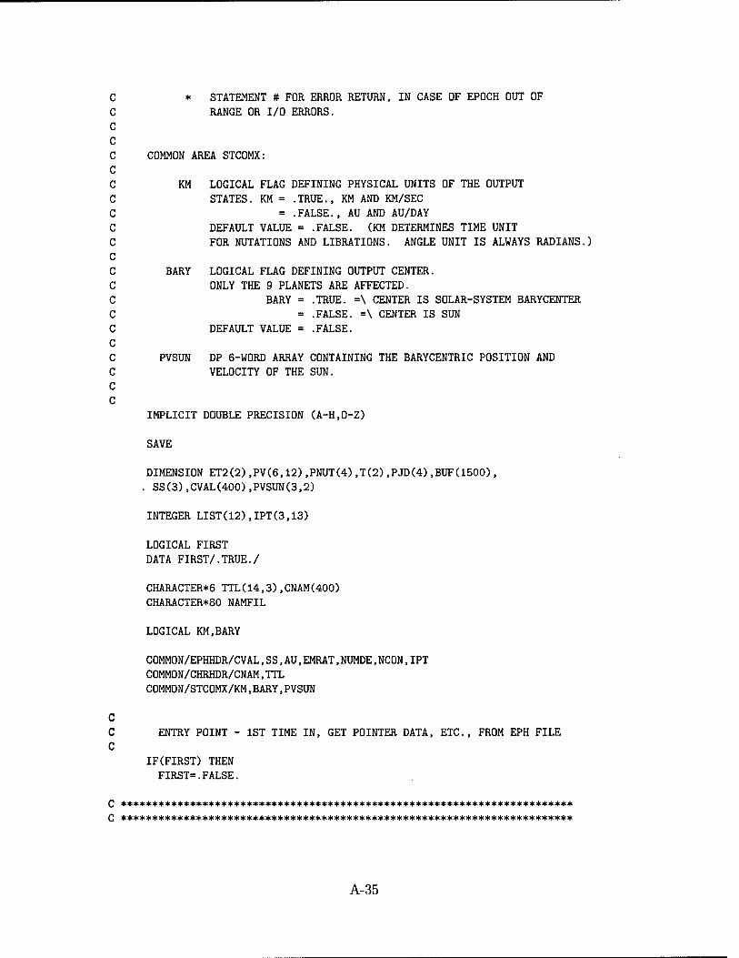
C * STATEMENT # FOR ERROR RETURN, IN CASE OF EPOCH OUT OF C RANGE OR I/O ERRORS. C C C COMMON AREA STCOMX: C C KM LOGICAL FLAG DEFINING PHYSICAL UNITS OF THE OUTPUT C STATES. KM = .TRUE., KM AND KM/SEC C = .FALSE., AU AND AU/DAY C DEFAULT VALUE = .FALSE. (KM DETERMINES TIME UNIT C FOR NUTATIONS AND LIBRATIONS. ANGLE UNIT IS ALWAYS RADIANS.) C C BARY LOGICAL FLAG DEFINING OUTPUT CENTER. C ONLY THE 9 PLANETS ARE AFFECTED. C BARY = .TRUE. =\ CENTER IS SOLAR-SYSTEM BARYCENTER C = .FALSE. =\ CENTER IS SUN C DEFAULT VALUE = .FALSE. C C PVSUN DP 6-WORD ARRAY CONTAINING THE BARYCENTRIC POSITION AND C VELOCITY OF THE SUN. C C
IMPLICIT DOUBLE PRECISION (A-H.O-Z)
SAVE
DIMENSION ET2(2),PV(6,12),PNUT(4),T(2),PJD(4),BUF(1500), . SS(3),CVAL(400),PVSUN(3,2)
INTEGER LIST(12),IPT(3,13)
LOGICAL FIRST DATA FIRST/.TRUE./
CHARACTER*6 TTL(14,3),CNAM(400) CHARACTER*80 NAMFIL
LOGICAL KM,BARY
COMMON/EPHHDR/CVAL,SS,AU,EMRAT,NUMDE,NCON,IPT COMMON/CHRHDR/CNAM,TTL COMMON/STCOMX/KM,BARY,PVSUN
C C ENTRY POINT - 1ST TIME IN, GET POINTER DATA, ETC., FROM EPH FILE C
IF(FIRST) THEN FIRST=.FALSE.
A-35
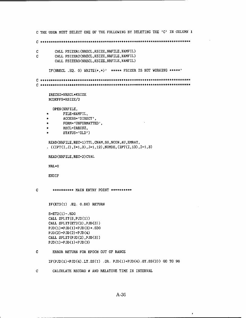
C THE USER MUST SELECT ONE OF THE FOLLOWING BY DELETING THE 'C IN COLUMN 1
Q *********************************************************************
C CALL FSIZERKNRECL.KSIZE.NRFILE.NAMFIL) C CALL FSIZER2(NRECL,KSIZE,NRFILE,NAMFIL)
CALL FSIZER3(NRECL,KSIZE,NRFILE,NAMFIL)
IF(NRECL .EQ. 0) WRITE(*,*)' ***** FSIZER IS NOT WORKING *****'
C ************************************************************************
c ************************************************************************
IRECSZ=NRECL*KSIZE NC0EFFS=KSIZE/2
OPENCNRFILE, * FILE=NAMFIL, * ACCESS='DIRECT', * FORM='UNFORMATTED', * RECL=IRECSZ, * STATUS='OLD')
READ(NRFILE,REC=1)TTL,CNAM,SS)NC0N,AU,EMRAT) . ((IPT(I,J),I=1,3),J=1,12))NUMDE,(IPT(I,13),I=113)
READ(NRFILE,REC=2)CVAL
NRL=0
ENDIF
C ********** MAIN ENTRY POINT **********
IF(ET2(1) .EQ. O.DO) RETURN
S=ET2(1)-.5D0 CALL SPLIT(S,PJD(D) CALL SPLIT(ET2(2),PJD(3)) PJD(1)=PJD(1)+PJD(3)+.5D0 PJD(2)=PJD(2)+PJD(4) CALL SPLIT(PJD(2),PJD(3)) PJD(1)=PJD(1)+PJD(3)
C ERROR RETURN FOR EPOCH OUT OF RANGE
IF(PJD(1)+PJD(4).LT.SS(1) .OR. PJD(1)+PJD(4).GT.SS(2)) GO TO 98
C CALCULATE RECORD # AND RELATIVE TIME IN INTERVAL
A-36
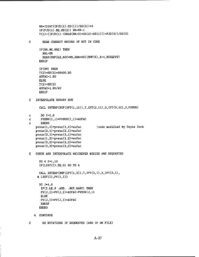
NR=IDINT((PJD(l)-SS(l))/SS(3))+3 IF(PJD(1).EQ.SS(2)) NR=NR-1 T(1)=((PJD(1)-(DBLE(NR-3)*SS(3)+SS(1)))+PJD(4))/SS(3)
C READ CORRECT RECORD IF NOT IN CORE
IF(NR.NE.NRL) THEN NRL=NR READ(NRFILE,REC=NR,ERR=99)(BUF(K),K=1.NCOEFFS)
ENDIF
IF(KM) THEN T(2)=SS(3)*86400.D0 AUFAC=l.DO ELSE T(2)=SS(3) AUFAC=l.DO/AU ENDIF
C INTERPOLATE SSBARY SUN
CALL INTERP(BUF(IPT(1,11)),T,IPT(2,11),3,IPT(3,11),2,PVSUN)
c DO 1=1,6 c PVSUN(I,1)=PVSUN(I,1)*AUFAC c ENDDO
pvsun(l,l)=pvsun(l,l)*aufac Icode modified by Dayne Cook pvsun(2,l)=pvsun(2,l)*aufac pvsun(3,l)=pvsun(3,l)*aufac pvsun(l,2)=pvsun(l,2)*aufac pvsun(2,2)=pvsun(2,2)*aufac pvsun(3,2)=pvsun(3,2)*aufac
C CHECK AND INTERPOLATE WHICHEVER BODIES ARE REQUESTED
DO 4 1=1,10 IF(LIST(I).EQ.O) GO TO 4
CALL INTERP(BUF(IPT(1,I)),T,IPT(2,I),3,IPT(3,I), & LIST(I),PV(1,D)
DO J=l,6 IFU.LE.9 .AND. .NOT.BARY) THEN PV(J,I)=PV(J,I)*AUFAC-PVSUN(J,1) ELSE PV(J,I)=PV(J,I)*AUFAC ENDIF
ENDDO
4 CONTINUE
C DO NUTATIONS IF REQUESTED (AND IF ON FILE)
A-37
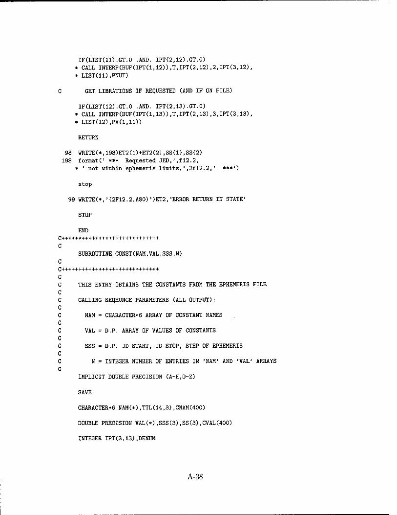
IF(LIST(ll).GT.O .AND. IPT(2,12).GT.O) * CALL INTERP(BUF(IPT(1,12)),T,IPT(2,12),2,IPT(3,12), * LIST(ll).PNUT)
C GET LIBRATIONS IF REQUESTED (AND IF ON FILE)
IF(LIST(12).GT.O .AND. IPT(2,13).GT.O) * CALL INTERP(BUF(IPT(1,13)),T,IPT(2,13),3,IPT(3,13), * LIST(12),PV(1,11))
RETURN
98 WRITE(*,198)ET2(1)+ET2(2),SS(1),SS(2) 198 formatC *** Requested JED,',f12.2,
* ' not within ephemeris limits,',2f12.2,' ***')
stop
99 WRITE(*,'(2F12.2,A80),)ET2,'ERROR RETURN IN STATE'
STOP
END C+++++++++++++++++++++++++++++ C
SUBROUTINE CONST(NAM,VAL.SSS.N)
C C THIS ENTRY OBTAINS THE CONSTANTS FROM THE EPHEMERIS FILE C C CALLING SEQEUNCE PARAMETERS (ALL OUTPUT): C C NAM = CHARACTER*6 ARRAY OF CONSTANT NAMES C C VAL = D.P. ARRAY OF VALUES OF CONSTANTS C C SSS = D.P. JD START, JD STOP, STEP OF EPHEMERIS C C N = INTEGER NUMBER OF ENTRIES IN 'NAM' AND 'VAL' ARRAYS C
IMPLICIT DOUBLE PRECISION (A-H.O-Z)
SAVE
CHARACTER+6 NAM(*),TTL(14,3),CNAM(400)
DOUBLE PRECISION VAL(*),SSS(3),SS(3),CVAL(400)
INTEGER IPT(3,13),DENUM
A-38
COMMON/EPHHDR/CVAL,SS,AU,EMRAT,DENUM,NCON,IPT COMMON/CHRHDR/CNAM,TTL
C CALL STATE TO INITIALIZE THE EPHEMERIS AND READ IN THE CONSTANTS
CALL STATE(O.DO,0,O.DO,O.DO)
N=NCON
DO 1=1,3 SSS(I)=SS(I) ENDDO
DO 1=1,N NAM(I)=CNAM(I) VAL(I)=CVAL(I) ENDDO
RETURN END
A-39
Bibliography
1. Baker, Robert M.L. Astrodynamics: Applications and Advanced Topics. New York: Academic Press, 1967.
2. Bar-Sever, Yoaz. Orbit Determination Accuracy Requirements for Collision Avoidance. AAS Paper 01-181, Santa Barbara CA: AAS/AIAA Space Flight Mechanics Conference, Feb 2001.
3. Bate, Roger R., Donald D. Mueller and Jerry E. White. Fundamentals of As- trodynamics. New York and London: Dover Publications, 1971.
4. "Boeing Inertial Upper Stage Defense Support Program Mission." Boeing Com- pany, http://www.boeing.com/defense-space/space/ius, November 2000.
5. Bowman, W. Jerry, Kenneth A. Carpenter and Christopher P. Chaplin. "Non- chemical Propulsion." Written by the Aerospace Engineering Department at the Air Force Institute of Technology, Wright-Patterson AFB OH, Spring 1994.
6. Bowman, Bruce R., William N. Barker and William G. Schick. Orbit Perturba- tion Analysis of West Ford Needles Clusters. Technical Report AIAA-2000-4236, Schriever AFB CO: Space Warfare Center, 2000. Printed by the American In- stitute of Aeronautics and Astronautics.
7. Bryant, Robert W. The Effect of Solar Radiation Pressure on the Motion of an Artificial Satellite. Technical Note NASA TN D-1063, National Aeronautics and Space Administration, September 1961.
8. Chobotov, Vladimir A. Spacecraft Attitude Dynamics and Control. Orbit Foun- dation Series, Malabar FL: Krieger Publishing Company, 1991.
9. Chobotov, Vladimir A., editor. Orbital Mechanics (Second Edition). AIAA Ed- ucation Series, Reston VA: American Institute of Aeronautics and Astronautics, 1996.
10. Clark, Phillip, editor. Jane's Space Directory (Thirteenth Edition). Alexandria VA: Jane's Information Group Inc., 1997-1998.
11. "Defense Support Program Satellites Fact Sheet." United States Air Force, http://www.af.mil/news/factsheets/DefenseSupportProgramSatel.html, November 2000.
12. "DSP Block 14 Quicklook." National Aeronautics and Space Administration, http://msl.jpl.nasa.gov/QuickLooks/dsp3QL.html, November 2000.
13. Halliday, David and Robert Resnick. Fundamentals of Physics (Second Edition). New York: John Wiley and Sons Inc., 1981.
BIB-1
14. Harwood, N.M. and G.G. Swinerd. "Long-Periodic and Secular Perturbations to the Orbit of a Spherical Satellite Due to Direct Solar Radiation Pressure," Celestial Mechanics and Dynamical Astronomy, 62:71-80 (1995).
15. Humble, Ronald W., Gary N. Henry and Wiley J. Larson. Space Propulsion Analysis and Design (First-revised Edition). Space Technology Series, New York: McGraw-Hill Companies Inc., 1995.
16. Jenkin, A.B. and R.A. Gick. Analysis of the Collision Risk Associated with GPS Disposal Orbit Instability. AAS Paper 01-115, Santa Barbara CA: AAS/AIAA Space Flight Mechanics Conference, Feb 2001.
17. Kelso, Thomas S. "Orbit Propagation: Part II," Satellite Times, i(4):80-81 (March/April 1995).
18. Koskela, P.E. "Orbital Effects of Solar Radiation Pressure on an Earth Satellite," The Journal of the Astronautical Sciences, iX(3):71-82 (1962).
19. Kubo-oka, T. "Long-Term Effect of Solar Radiation on the Orbit of an Octagonal Satellite Orbiting Around the Moon," Advances in Space Research, 23 (A):727- 731 (1999).
20. Luthcke, S.B., J.A. Marshall and S.C. Rowton. "Enhanced Radiative Force Modeling of the Tracking and Data Relay Satellites," The Journal of the Astro- nautical Sciences, ^5(3):349-370 (July-September 1997).
21. Luu, Kim and Chris Sabol. Effects of Perturbations on Space Debris in Su- persynchronous Storage Orbits. Technical Report AFRL-VS-PS-TR-1998-1093, Kirtland AFB NM: Air Force Research Laboratory, October 1998.
22. Marshall, J.A., P.G. Antreasian and G.W. Rosborough. Modeling Radiation Forces Acting on Satellites for Precision Orbit Determination. AAS Paper 91- 357, San Diego CA: American Astronautical Society, 1991.
23. Milani, Andrea, Anna Maria Nobili and Paolo Farinella. Non-Gravitational Per- turbations and Satellite Geodesy. Bristol, UK: Adam Hilger, 1987.
24. Perturbation Models. NORAD Technical Publication SCC 008, Schriever AFB CO: Space Warfare Center, April 1982.
25. "Planetary Orbital Elements." National Aeronautics and Space Administration, http://ssd.jpl.nasa.gov/elemplanets.html, November 2000.
26. Press, William H., Brian P. Flannery and Saul A. Teukolsky. Numerical Recipes (FORTRAN Version). New York: Cambridge University Press, 1989.
27. Ries, J.C., C.K. Shum and B.D. Tapley. "Surface Force Modeling for Precision Orbit Determination," Geophysical Monograph 73, IUGG Vol 13, Environmental Effects on Spacecraft Positioning and Trajectories:111—124 (1993).
28. Sabol, Chris, Scott Carter and Megan Bir. Analysis of Preselected Orbit Gener- ator Options for the Draper Semianalytic Satellite Theory. Technical Report
BIB-2
AIAA-2000-4231, Kirtland AFB NM: Air Force Research Laboratory, 2000. Printed by the American Institute of Aeronautics and Astronautics.
29. Solar Events: Solar Eclipse Predictions. Technical Order CG-SCF-225C, Schriever AFB CO: Third Space Operations Squadron, December 1989.
30. Spencer, David. Covariance Generation for Space Objects Using Public Data. AAS Paper 01-113, Santa Barbara CA: AAS/AIAA Space Flight Mechanics Conference, Feb 2001.
31. Springer, T.A., G. Beutler and M. Rothacher. "A New Solar Radiation Pressure Model for GPS," Advances in Space Research, 23(4):673-676 (1999).
32. Tascione, Thomas F. Introduction to the Space Environment (Second Edition). Orbit Foundation Series, Malabar FL: Krieger Publishing Company, 1994.
33. Vokrouhlicky, D. and P. Farinella. "Radiative Forces and LAGEOS' Orbit," Advances in Space Research, i£(12):(12)15-(12)19 (1995).
34. Vokrouhlicky, D., P. Farinella and F. Mignard. "Solar Radiation Pressure Per- turbations for Earth Satellites: I. A complete theory including penumbra tran- sitions," Astronomy and Astrophysics, 280:295-312 (1993).
35. Vokrouhlicky, D., P. Farinella and F. Mignard. "Solar Radiation Pressure Per- turbations for Earth Satellites: II. An approximate method to model penumbra transitions and their long-term orbital effects on LAGEOS," Astronomy and Astrophysics, 255:333-343 (1994).
36. Vokrouhlicky, D., P. Farinella and F. Mignard. "Solar Radiation Pressure Per- turbations for Earth Satellites: IV. Effects of the Earth's polar flattening on the shadow structure and the penumbra transitions," Astronomy and Astrophysics, 507:635-644 (1996).
37. Wertz, James R. and Wiley J. Larson, editors. Space Mission Analysis and Design (Third Edition). Space Technology Series, Torrance CA: Microcosm Press, 1999.
38. Wiesel, William E. Spaceflight Dynamics (Second Edition). Boston MA: Irwin/McGraw-Hill, 1997.
39. Woodburn, J. Effects of Eclipse Boundary Crossings on the Numerical Inte- gration of Orbit Trajectories. Technical Report AIAA-2000-4027, Analytical Graphics, Inc., 2000. Printed by the American Institute of Aeronautics and Astronautics.
BIB-3
Vita
Major Dayne G. Cook was born and raised in Payson, Utah. He graduated
valedictorian from Payson High School in 1982. He entered undergraduate studies
at Brigham Young University in Provo, Utah where he graduated with a Bachelor of
Science degree in Computer Science in December 1988, and was then commissioned
through AFROTC. During his college years, he served as a proselyting missionary
for The Church of Jesus Christ of Latter-day Saints in Seoul, South Korea from 1983
to 1985. Major Cook's first Air Force assignment was to Undergraduate Space Train-
ing at Lowry AFB, Colorado, after which he was assigned to the 4th Space Warning
Squadron at Holloman AFB, New Mexico, as a Space Operations Crew Comman-
der. Other positions held while at Holloman AFB include Flight Operations Control
Officer and Deputy Chief of Training. In January 1993, he relocated to Colorado
Springs where he served one year as an AFSPACECOM Consolidated Operations
Center Crew Commander at Schriever AFB. Continuing his tour at Schriever AFB,
he then went on to become the Chief, Orbit Analysis Section at the 3rd Space Oper-
ations Squadron, followed by duty as a Flight Commander in the same squadron. In
November 1996, he returned to Korea to serve as Security Engineer and C2 Require-
ments Officer in J6 Information Systems, United States Forces Korea at Yongsan
Army Garrison, Seoul, Republic of Korea (ROK). After 18 months, his Korean lan-
guage training earned him the position of Aide-de-Camp to the Commander, ROK
Air Force Operations Command, 7th Air Force, Osan AB, Republic of Korea. He
entered the Space Operations Program, Graduate School of Engineering and Man-
agement, Air Force Institute of Technology, in August 1999. Upon graduation, Major
Cook will be assigned to Air Force Space Command Headquarters, Peterson AFB,
Colorado.
VITA-1
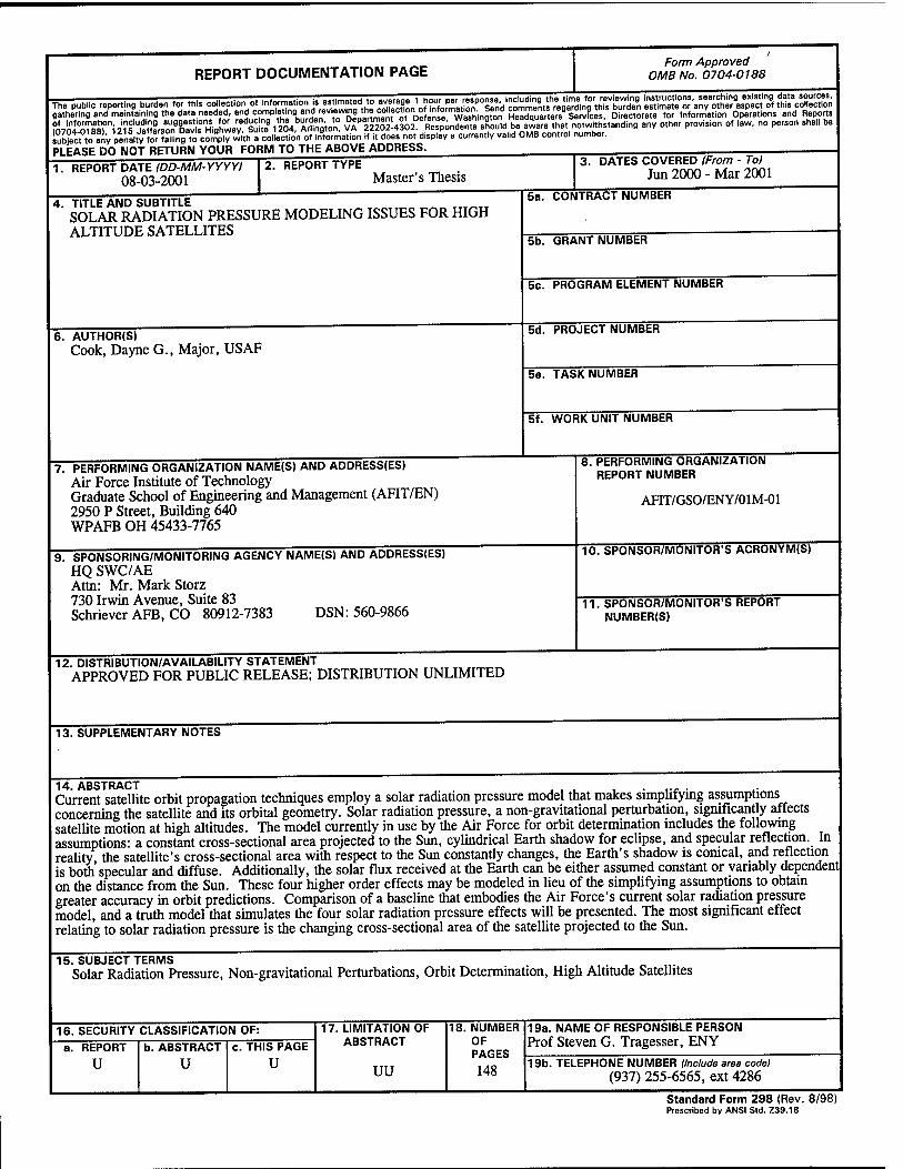
REPORT DOCUMENTATION PAGE Form Approved
OMB No. 0704-0188
The public reporting burden for «hi. collection of Information is »time.ed to ,.verage 1 *™%£V™%1 ^l^jaS^^^ffa gathering and maintaining the data needed. °"^°7'0«nS^ HeadquartersÄces SSrectorate for Information Operations and Reports SUÄ? mtÄs3" VDra2r22^!4§02DeSondem^nou,d be alre that notwithstanding any other provision of law, no person shall be iubteot to8any penaltZ ?aiLg to »mplywhh a collection of information if it does not display a currently vahd OMB contro! number. PLEASE DO NOT RETURN YOUR FORM TO THE ABOVE ADDRESS. 1. REPORT DATE (DD-MM-YYYY)
08-03-2001 2. REPORT TYPE
Master's Thesis
4. TITLE AND SUBTITLE SOLAR RADIATION PRESSURE MODELING ISSUES FOR HIGH ALTITUDE SATELLITES
6. AUTHOR(S) Cook, Dayne G., Major, USAF
7. PERFORMING ORGANIZATION NAME(S) AND ADDRESS(ES) Air Force Institute of Technology Graduate School of Engineering and Management (AFIT/EN) 2950 P Street, Building 640 WPAFB OH 45433-7765
3. DATES COVERED (From - To) Jun 2000 - Mar 2001
5a. CONTRACT NUMBER
5b. GRANT NUMBER
5c. PROGRAM ELEMENT NUMBER
5d. PROJECT NUMBER
5e. TASK NUMBER
5f. WORK UNIT NUMBER
9. SPONSORING/MONITORING AGENCY NAME(S) AND ADDRESS(ES) HQ SWC/AE Atta: Mr. Mark Storz 730 Irwin Avenue, Suite 83 Schriever AFB, CO 80912-7383 DSN: 560-9866
8. PERFORMING ORGANIZATION REPORT NUMBER
AFIT/GSO/ENY/01M-01
10. SPONSOR/MONITOR'S ACRONYM(S)
11. SPONSOR/MONITOR'S REPORT NUMBER(S)
12. DISTRIBUTION/AVAILABILITY STATEMENT APPROVED FOR PUBLIC RELEASE; DISTRIBUTION UNLIMITED
13. SUPPLEMENTARY NOTES
In
14. ABSTRACT J , , . ... . Current satellite orbit propagation techniques employ a solar radiation pressure model that makes simplifying assumptions concerning the satellite and its orbital geometry. Solar radiation pressure, a non-gravitational perturbation, significantly affects satellite motion at high altitudes. The model currently in use by the Air Force for orbit determination mcludes the following assumptions: a constant cross-sectional area projected to the Sun, cylindrical Earth shadow for eclipse, and specular reflection, reality the satellite's cross-sectional area with respect to the Sun constantly changes, the Earth's shadow is conical, and reflection is both'specular and diffuse. Additionally, the solar flux received at the Earth can be either assumed constant or variably dependent on the distance from the Sun. These four higher order effects may be modeled in lieu of the simplifying assumptions to obtain greater accuracy in orbit predictions. Comparison of a baseline that embodies the Air Force's current solar radiation pressure model, and a truth model that simulates the four solar radiation pressure effects will be presented. The most significant effect relating to solar radiation pressure is the changing cross-sectional area of the satellite projected to the Sun.
15. SUBJECT TERMS Solar Radiation Pressure, Non-gravitational Perturbations, Orbit Determination, High Altitude Satellites
16. SECURITY CLASSIFICATION OF: REPORT
u b. ABSTRACT
U c. THIS PAGE
U
17. LIMITATION OF ABSTRACT
uu
18. NUMBER OF PAGES 148
19a. NAME OF RESPONSIBLE PERSON Prof Steven G. Tragesser, ENY 19b. TELEPHONE NUMBER (Include area code)
(937) 255-6565, ext 4286
Standard Form 298 (Rev. 8/98) Prescribed by ANSI Std. Z39.18