Solar Radiation Theory - DiVA portaluu.diva-portal.org/smash/get/diva2:1305017/FULLTEXT01.pdf2.2 Planck’s radiation law In order to understand the properties of the solar radiation

Solar Radiation Theory

Joakim Widen and Joakim MunkhammarDepartment of Engineering Sciences

Uppsala University

Solar Radiation Theory, Uppsala University 2019.

Copyright c© Joakim Widen and Joakim Munkhammar 2019.

ISBN 978-91-506-2760-2

DOI 10.33063/diva-381852

URN http://urn.kb.se/resolve?urn=urn:nbn:se:uu:diva-381852

Cover figure: The front page of Opticae Thesaurus from 1572, showing ships set on firewith the help of parabolic mirrors, an application of solar irradiance first attributed bylegend to the greek astronomer and mathematician Archimedes. The image also showsother optical phenomena such as a rainbow and distorted images due to refraction inwater. (Image from Wikimedia Commons, public domain.)

Contents 1

Contents

Preface 5

1 Introduction 7

2 Black-body radiation and the Sun 9

2.1 The source of solar energy . . . . . . . . . . . . . . . . . 9

2.2 Planck’s radiation law . . . . . . . . . . . . . . . . . . . 10

2.3 The solar constant . . . . . . . . . . . . . . . . . . . . . 13

2.4 Categorization of radiation . . . . . . . . . . . . . . . . . 15

3 Available solar radiation on Earth 17

3.1 Atmospheric attenuation . . . . . . . . . . . . . . . . . . 17

3.2 Air mass . . . . . . . . . . . . . . . . . . . . . . . . . . . 18

3.3 Radiation components . . . . . . . . . . . . . . . . . . . 19

3.4 Temporal and geographical variations in solar energy avail-ability . . . . . . . . . . . . . . . . . . . . . . . . . . . . 21

3.5 Earth’s energy balance . . . . . . . . . . . . . . . . . . . 25

4 Quantifying available solar energy on planar surfaces 27

4.1 Measured solar irradiance data . . . . . . . . . . . . . . . 28

4.2 Solar time . . . . . . . . . . . . . . . . . . . . . . . . . . 30

2 Contents

4.3 Solar angles . . . . . . . . . . . . . . . . . . . . . . . . . 31

4.4 Extraterrestrial radiation . . . . . . . . . . . . . . . . . . 33

4.5 Beam radiation on tilted surfaces . . . . . . . . . . . . . 34

4.6 Diffuse radiation on tilted surfaces . . . . . . . . . . . . . 35

4.7 Ground-reflected radiation . . . . . . . . . . . . . . . . . 37

4.8 Complete model for tilted plane global radiation . . . . . 37

4.9 Some notes on optimization of surface orientation . . . . 37

5 Exercises 39

A Derivation of the incidence angles of beam radiation 45

A.1 Zenith angle of incidence . . . . . . . . . . . . . . . . . . 45

A.2 Incidence angle on an arbitrarily oriented plane . . . . . 47

Nomenclature 3

Nomenclature

Symbol Description Value Unit

a First Angstrom coefficient – –Ai Anisotropy index – –b Second Angstrom coefficient – –c Speed of light in vacuum 2.998× 108 ms−1

d Day of year – –fview View factor – –G0n, G0 Extraterrestrial radiation, nor-

mal and on horizontal plane– Wm−2

Gb Total blackbody radiation – Wm−2

Gbλ Wavelength distribution ofblackbody radiation

–Wm−2µm−1

Gc Clear-sky irradiance – Wm−2

Gsc Solar constant 1367 Wm−2

h Planck’s constant 6.626× 10−34 JsH Total monthly irradiation – kWhm−2

Hc Total monthly clear-sky irradia-tion

– kWhm−2

I0 Extraterrestrial radiation onhorizontal plane over a time in-terval

– Wm−2

I, IT Global radiation on horizontaland tilted planes over a timeinterval

– Wm−2

4 Nomenclature

Symbol Description Value Unit

Ib, IbT Beam radiation on horizontaland tilted planes over a time in-terval

– Wm−2

Id, IdT Diffuse radiation on horizontaland tilted planes over a time in-terval

– Wm−2

IgT Ground-reflected radiation ontilted plane over a time interval

– Wm−2

k Boltzmann’s constant 1.380× 10−23 JK−1

Lloc Local meridian – ◦

Lst Standard meridian – ◦

m Air mass – –n Refractive index – –Rb Geometric factor – –S Fraction of bright sunshine hours – –ts Solar time – mintst Standard clock time – minT Temperature – Kβ Tilt angle – ◦

δ Declination – ◦

γ Azimuth angle – ◦

κ Clear-sky index – –λ Wavelength of electromagnetic

radiation– µm

ω Hour angle – ◦

φ Latitude – ◦

Φbλ Wavelength distribution of pho-ton flux

– s−1m−2µm−1

ρg Albedo of the ground – –σ Stefan-Boltzmann constant 5.670× 10−8 Wm−2K−4

θz Angle of incidence on tiltedplane

– ◦

θz Zenith angle of incidence – ◦

Preface 5

Preface

One of the challenges in solar engineering is that the availability of thesolar resource varies with time and location. An important engineeringtask is to design solar energy systems that are able to collect as muchsolar radiation as possible under these constraints. This book introducesthe basic properties of solar radiation that are required to understandhow the solar resource can be converted into useful heat and electricity,and what the limitations are. It also shows how solar radiation on planarsurfaces can be modeled mathematically. This is useful when optimizingthe orientation of collecting surfaces and predicting the performance ofdifferent system designs. The book builds upon lecture notes from solarengineering courses at Uppsala University, carefully edited to suit a widerscientific and engineering audience. The two authors have, together,more than two decades’ experience of teaching, research and developmentin the field of solar irradiance modeling.

Chapter 1 gives a short historical background to utilization of solar ir-radiance. Chapter 2 reviews the most important concepts of black-bodyradiation and electromagnetic radiation. Chapter 3 gives an overviewof the availability of the solar resource on Earth. Chapter 4 providesthe mathematical framework for modeling solar energy availability onarbitrarily oriented, planar surfaces, based on measurements in the hor-izontal plane. Review questions on the content as well as exercises areincluded in chapter 5. Additionally, a derivation of the incidence anglesof beam radiation (not commonly explained in the available literature)is presented in the appendix.

Uppsala, April 2019Joakim Widen and Joakim Munkhammar

6 Preface

Chapter 1. Introduction 7

Chapter 1

Introduction

The Sun has played an important role in human cultures throughouthistory. Archaeological sources provide glimpses of sun-worshipping inprehistoric societies and of early astronomical records in Mesopotamiancivilizations. The abundance of the Sun’s energy and its seasonal avail-ability have naturally set the limits of human life and societal prosperityand growth, governing the turn of seasons and the wheel of the yearin agrarian societies. However, direct use of solar radiation for specificpurposes such as heating and providing power, made its appearance rel-atively late in history. The Greeks were aware of various optical phe-nomena, and Archimedes is said to have used parabolic mirrors, perhapshighly polished bronze or copper shields, to put fire to Roman enemyships outside Syracuse in 212 B.C.,1 but more practical use of solar en-ergy came with the scientific revolution [1, p. 386].

Starting in the 17th century, attempts were made not only to concentratesunlight but to also make it perform mechanical work. In the beginning ofthe century, french physicist Salomon de Caus constructed the first proto-type for a sun-fuelled steam engine using concentrating lenses. However,these devices would be more accurately described as toys than usablemachines. In 1861 Augustin Mouchot, a French mathematics teacher,

1In the 18th century French naturalist Georges Buffon attempted a reconstructionof the Archimedean myth and apparently managed to set fire to an old house usingaround 150 mirrors at a distance of 60 meters. More modern reconstructions were madeboth in 1992 and 2005, concluding that the effectiveness of the mirror tactic would havebeen minor both in terms of manpower and inflicted damage [1].

8 Chapter 1. Introduction

managed to produce enough steam to drive a small engine. After yearsof research and development he succeeded in producing an engine largeenough to power a printing press, which was presented to the world atthe Universal Exhibition in Paris in 1878. Even if widespread use ofsolar power was to take another one hundred-odd years to emerge, thetechnology for producing mechanical work with the help of the Sun wasin place [1, p. 389].

The technology for producing solar electricity was also in place, by addinga generator to Mouchot’s engine. In fact, the first solar power plant wentinto construction in Egypt in 1912, but after the First World War oiland coal provided more competitive means of producing electric power.Instead, a completely different technology was to harness the solar ir-radiance on a large scale. Soon after a breakthrough with silicon solarcells at Bell Labs in the U.S. the first commercial photovoltaic (PV)panels, called ”Solar Batteries”, were produced in the 1950s [1, pp. 392-394]. The devices soon found their use in various products, ranging frompocket calculators to satellites, but it was after massive subsidy schemeswere introduced in Germany and Japan in the 1990s that rooftop PVsystems connected to the power grid began to get widely used. Marketsexpanded, prices gradually dropped and solar power began making itsway into power systems.

For all of these solar-powered devices, the properties of solar radiationset the operational constraints. In the following chapters, we will giveyou an understanding of basic solar radiation theory and how to use itfor quantifying the solar energy on any device, be it a polished bronzemirror or a utility-scale solar power plant.

Chapter 2. Black-body radiation and the Sun 9

Chapter 2

Black-body radiation and the Sun

This section reviews the fundamentals of electromagnetic and black-bodyradiation that are required to understand the nature of the Sun and ofthe solar radiation that reaches Earth. It also defines some importantconcepts that are useful for practical applications of solar radiation.

2.1 The source of solar energy

The Sun, our closest star, is a spherical gaseous self-gravitating bodyconsisting mainly of hydrogen. It is located at the center of the solarsystem, on average 1.5 × 1011 m from Earth. At the inner core of theSun, the gravitational force creates a pressure which generates nuclearfusion that turns hydrogen into helium. In this process a portion of themass is converted into an abundant amount of electromagnetic radiation,which makes the Sun the dominant source of radiative energy in thesolar system. The Sun has a complex physical structure and consistsof several regions, from the dense inner core to the outer atmosphericallayer, the corona. Both the corona and the core are very hot, in theorder of 106 − 107 K, while the intermediate regions that transport andemit energy as outgoing radiation are cooler (although hot by earthlystandards).

Energy from fusion reactions in the Sun’s interior is transported throughsuccessive convection, radiation, absorption, emission and reradiation tothe Sun’s equivalent of a surface, the photosphere, which absorbs and

10 Chapter 2. Black-body radiation and the Sun

emits a continuous spectrum of radiation. The photosphere is the sourceof most visible radiation reaching Earth. It has a surface temperature,or, more correctly, an effective black-body temperature of 5777 K (this isthe temperature of a black-body radiating the same amount of energy asthe Sun). Although it consists of several absorbing and emitting layersand has a considerable temperature gradient across its radius, the Sunclosely resembles the ideal concept of a black-body, the properties ofwhich will be explored in the next section.

2.2 Planck’s radiation law

In order to understand the properties of the solar radiation reachingEarth, it is useful to review some concepts of electromagnetic radiationand the properties of black-bodies. Electromagnetic radiation can be re-garded as a wave, characterized by its wavelength λ. All electromagneticradiation travels at the speed of light c (2.998×108 m/s) in a vacuum (orc/n in a material with refractive index n) and has a frequency ν such thatc = λν. By quantum mechanics, electromagnetic radiation can also beregarded as a flux of photons, where the energy content in each photondepends on the frequency. In electromagnetic radiation with a certainwavelength λ a photon has the energy

E = hν =hc

λ(2.1)

where h is Planck’s constant (6.626× 10−34 Js).

The radiation emitted from a hot object like the Sun, or any objectfor that matter, is distributed over a range of wavelengths and, conse-quently, consists of a flux of photons with different energy content. Thedistribution of radiated energy over wavelengths, as well as the totalenergy flux, depends on the temperature of the object. This can be ap-proximated with a black-body, which is an idealized state of an objectin thermodynamical equilibrium, where the object is a perfect absorberand emitter of radiation. That is, it absorbs all the radiation incident onit and emits the maximum possible amount of radiation. Based on bothquantum mechanics and thermodynamics a black-body can be described


by Planck’s radiation law, where the wavelength distribution of radiationemitted from a black-body with temperature T is given by:

Gbλ =2πhc2

λ5(e

hcλkT − 1

) (2.2)

where k is Boltzmann’s constant (1.380×10−23 JK−1). Gbλ is often givenin units of Wm−2µm−1. We can also express this distribution in termsof photon flux by dividing the emitted power at each wavelength by thecorresponding photon energy:

Φbλ =λ

hcGbλ (2.3)

in units of s−1m−2µm−1. By differentiating the distribution in Equa-tion 2.2 with respect to wavelength and equating to zero, the wavelengthcorresponding to the maximum of the distribution can be found. Therelation between this wavelength and the black-body temperature is

λmaxT = 2897.8 µmK (2.4)

which is known as Wien’s displacement law and states that the maxi-mum wavelength is inversely proportional to the temperature. Anotheruseful relation, which can be obtained by integrating Planck’s law overall wavelengths, is the Stefan-Boltzmann equation. It expresses the totalemitted black-body radiation:

Gb =

∫ ∞0

Gbλdλ = σT 4 (2.5)

where σ is the Stefan-Boltzmann constant (5.670× 10−8 Wm−2K−4). Gb

is in units of Wm−2. Note that this is also the unit most often used forincident solar radiation.

The latter two equations tell us something fundamental and familiarabout heated objects: the Stefan-Boltzmann equation shows that thetotal radiated power increases with the temperature of the object andWien’s displacement law shows that the peak wavelength decreases withincreasing temperature, which, for example, causes metals to glow brighteras they get hotter.


0 0.2 0.4 0.6 0.8 1 1.2 1.4 1.6 1.8 2Wavelength ( m)

0

1

2

3

4

5

6

7

8

9

10

Spe

ctra

l em

issi

ve p

ower

(W

/m2

m)

107

T = 6000 K

T = 5000 K

T = 4000 K

(a)

0 2 4 6 8 10 12 14 16 18 20Wavelength ( m)

102

104

106

108

Spe

ctra

l em

issi

ve p

ower

(W

/m2

m)

T = 6000 K

T = 400 K

(b)

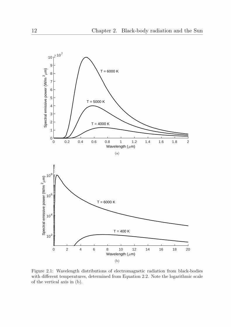
Figure 2.1: Wavelength distributions of electromagnetic radiation from black-bodieswith different temperatures, determined from Equation 2.2. Note the logarithmic scaleof the vertical axis in (b).


These two properties of black-body radiation are shown in Figures 2.1(a)and 2.1(b). Both figures show the spectral distribution of the thermalradiation from a black-body with a temperature of 6000 K (approxi-mately the surface temperature of the Sun). If the Sun were a trueblack-body, this is what we would expect its radiation distribution tolook like. The figures also show black-body radiation curves at lowertemperatures. Figure 2.1(b) (note the scale on the y-axis) clearly showsthe difference between radiation from a black-body with a temperatureof 6000 K and one with 400 K (127 ◦C), which is closer to temperaturesencountered in our daily environment.

2.3 The solar constant

Let us now turn to the actual solar radiation that reaches Earth’s atmo-sphere. How much radiation is there and how is it distributed over thewavelengths? To start with, we note that solar radiation levels in thesolar system drop with the square of the distance to the Sun. To real-ize this, assume that the Sun’s radius is r and its surface temperatureT . The surface area of the Sun is then 4πr2 and the total radiative fluxfrom the Sun is, using the Stefan-Boltzmann equation, σT 4×4πr2. Now,the surface of a larger imaginary sphere with radius l with the Sun atits center will receive the same amount of radiation, but over the largerarea 4πl2. Consequently, the energy flux per unit area at the distance lfrom the Sun is

Gl =σT 4 × 4πr2

4πl2= σT 4

(rl

)2. (2.6)

If you use the black-body temperature of the Sun (5777 K), the radiusof the Sun (6.957× 108 m) and the distance between the Sun and Earth(1.495 × 1011 m), you will get the average radiative flux just outsideEarth’s atmosphere, per unit area facing the Sun: 1367 W/m2. This willbe denoted by Gsc and is called the solar constant, or the air mass zero(AM0) radiation.

Gsc is not determined experimentally in this way but the other wayaround: it is the Sun’s surface temperature that is inferred from mea-surements ofGsc at Earth by using Equation 2.6 solved for the black-body


temperature T . Estimates of Gsc have gradually improved by radiationmeasurements outside the atmosphere using aircraft, ballons and space-craft. The value 1367 W/m2, adopted by the World Radiation Center(WRC), is commonly used in the solar engineering literature [2].

Through measurements it is also possible to determine the spectral distri-bution of the AM0 radiation. Figure 2.2 shows the standardized WRCspectral irradiance curve, obtained from high-altitude and space mea-surements. The spectral distribution of the AM0 radiation follows closelythe shape of the black-body radiation curve that is obtained from evalu-ating Planck’s law close to the surface temperature of the Sun (cf. Fig-ure 2.1). The dissimilarities in the spectral distributions are due toabsorption in the cooler, upper parts of the Sun’s photosphere.

0 200 400 600 800 1000 1200 1400 1600 1800 2000Wavelength (nm)

0

0.5

1

1.5

2

2.5

Sol

ar s

pect

ral i

rrad

ianc

e (W

/m2nm

)

Figure 2.2: The standard WRC spectrum of AM0 radiation. Data obtained fromNREL, USA [3].

Due to Earth’s elliptic orbit around the Sun the actual solar radiationoutside the atmosphere at a given time (the extraterrestrial radiation)will differ from Gsc. Over the year, it varies from 1412 W/m2 at thebeginning of July to 1322 W/m2 at the turn of the year; a 3.3% variation


from the mean value. This can be expressed mathematically as

G0n = Gsc

(1 + 0.033× cos

(360

d

365

))(2.7)

where d is the day of the year. The subscript 0 denotes zero air mass(AM0) and the subscript n indicates that the radiation is on a planenormal to the Sun-Earth axis.

2.4 Categorization of radiation

Based on properties and field of applications, electromagnetic radiationis categorized into wavelength bands. Figure 2.3 shows some commonclassifications in the ranges relevant for solar engineering purposes. Thevast majority of solar radiation is in the wavelength range of approxi-mately 0.3 to 3 µm and spans parts of the ultraviolet (UV) and infrared(IR) ranges. A simpler classification of the wavelengths of importancein solar engineering is to divide the spectrum of solar and IR radiationinto short-wave and long-wave radiation. Short-wave is the same as so-lar radiation and long-wave is everything with longer wavelengths. Forthe purpose of solar collectors it is a useful fact that the incident solarradiation in the short-wave range and the emitted radiation from solarcollectors in the long-wave ranges do not overlap significantly. This isbeneficial because it makes it possible to design materials and devicesthat have entirely different properties for short-wave solar and long-wavethermal radiation.


Visible, 0.4–0.8

Solar, 0.3–3

Infrared, 0.8–1000

Ultraviolet, 0.01–0.4

10–2 10–1 100 101 102 103

Wavelength (µm)

Figure 2.3: Some common wavelength bands in the spectrum of electromagnetic radi-ation.

Chapter 3. Available solar radiation on Earth 17

Chapter 3

Available solar radiation on Earth

Extraterrestrial radiation is affected in various ways during passage throughthe atmosphere. This section reviews these mechanisms and describesthe properties of the solar radiation available at Earth’s surface. A shortdiscussion on the radiation and energy balance of Earth is also included.

3.1 Atmospheric attenuation

When passing through the atmosphere, solar radiation with normal inci-dence is subject to two sources of attenuation: scattering and absorption.

Scattering occurs when the radiation interacts with air molecules, waterand dust in the atmosphere. The degree of scattering is determined bythe wavelength of the radiation in relation to particle size, the concen-tration of particles in the atmosphere and the total mass of air that theradiation has to travel through. The most important process is Rayleighscattering, in which light is scattered off air molecules. This type of scat-tering is most effective for shorter wavelengths in the blue end of thespectrum, mainly those shorter than 0.6 µm. This scattering processexplains the blue color of the sky at daytime, the yellow color of theSun and the reddening of the sky at night. This occurs because mostof the radiation reaching the ground from other directions than directlyfrom the Sun has been scattered by Rayleigh scattering. Note that asignificant amount of the scattered light is redirected back into space.

18 Chapter 3. Available solar radiation on Earth

Absorption of solar radiation occurs in the UV range due to ozone andin the IR range due to water and carbon dioxide. In the process ofabsorption, the solar radiation is converted to heat, which is emitted bythe particles as long-wave radiation.

The effect of Rayleigh scattering is quite large and wavelength-dependent,as can be seen in Figure 3.1.

0 200 400 600 800 1000 1200 1400 1600 1800 2000Wavelength (nm)

0

0.5

1

1.5

2

2.5

Sol

ar s

pect

ral i

rrad

ianc

e (W

/m2 nm

)

6000 K blackbody

AM0

AM1.5

Figure 3.1: The AM1.5 spectrum in relation to the AM0 spectrum and the 6000 K black-body radiation distribution weighted as in Equation 2.6. The drop in peak intensityat roughly 500 nm is due to Rayleigh scattering, the other dips are due to absorbtionfrom oxygen (O2), ozone (O3), water (H2O) and carbon dioxide (CO2). The AM1.5spectrum is specified by the National Renewable Energy Laboratory (NREL), USA [3].

3.2 Air mass

Attenuation of solar radiation depends on how far the radiation has totravel through the atmosphere. The longer the path length, the moreparticles the light has to interact with. This varies over the year andover individual days, with the longest path in the evenings, when theSun is close to the horizon. The path length is described by the airmass. Formally, air mass is the ratio of the atmospheric mass through


which the radiation passes from the Sun’s current position in the sky,to the mass that it would pass through if the Sun were at the zenith(directly overhead). For example, at air mass 2, the path length throughthe atmosphere is two times longer than if the Sun were directly overhead.If the zenith angle, i.e. the angle from overhead to the Sun, is denotedby θz, the air mass is to close approximation

m =1

cos θz(3.1)

θz < 70◦ as shown in Figure 3.2. For higher angles the curvature of Earthbecomes influential. For θz = 85◦ the error is 10%. A more thoroughdiscussion of air mass can be found in [4].

θz DDcos zθ

Figure 3.2: Atmospherical path length D of solar radiation at zenith angle θz.

Because the atmospheric conditions vary over time, a standard spectrumfor radiation at ground level is needed for development and testing of so-lar devices. The accepted standard is the distribution for m = 1.5, theAM1.5 spectrum, which corresponds to a zenith angle of 48.2◦. Figure 3.1shows the so-called AM1.5 spectrum and compares it to the extraterres-trial WRC spectrum and a 6000 K black-body distribution.

3.3 Radiation components

Because of scattering, radiation on Earth’s surface consists of two com-ponents. Part of the incoming radiation is preserved as beam radiation,


while the rest is scattered in the atmosphere and is either reflected backinto space or reaches the ground as diffuse radiation. In contrast to beamradiation, which has a well-defined direction, diffuse radiation originatesfrom all over the sky dome. Although diffuse radiation is most intensenear the Sun, a good approximation is to assume that it is isotropic, i.e.,uniformly distributed on all directions.

The proportions of diffuse and beam radiation are strongly dependenton weather conditions. In sunny weather with clear skies, some 10-20% of the radiation is diffuse. In cloudy weather with a lack of brightsunshine most of the incident radiation is diffuse. Figure 3.3 shows theseproportions on two days in Norrkoping, Sweden (59◦35′31” N 17◦11′8”E). Over the year, the total diffuse part can be significant. For example,in Norrkoping, between 1983 and 1998, the diffuse share of the totalradiation was 51% on average. As a comparison, in one of Sweden’smost sunny locations, Visby (57◦38′5” N 18◦17′57” E), the diffuse partwas still 47% for the same years [6].

00:00 12:00 24:00Time

0

200

400

600

800

1000

W/m

2

July 3, 2008

GlobalDiffuse

00:00 12:00 24:00Time

0

200

400

600

800

1000

W/m

2

July 8, 2008

GlobalDiffuse

Figure 3.3: Global and diffuse radiation on the horizontal plane in Norrkoping, Sweden,on two summer days in 2008, one clear day (left) with a few moving clouds in theafternoon and one completely overcast day (right). On the clear day the diffuse fractionwas 14.2%, on the overcast day it was 99.7%. Note that the time here is UTC, i.e.Swedish standard time minus one hour (minus two hours including summer daylightsavings time).

In addition, diffuse radiation has a different spectrum than beam radia-


tion. The high-frequency part of the spectrum is more pronounced be-cause Rayleigh scattering mainly affects shorter wavelengths. However,for most practical purposes the spectral distribution can be assumed tobe the same as for beam radiation.

A third radiation component that has to be considered in solar energyapplications is radiation reflected from the ground and from other sur-rounding objects onto a sloped surface. It depends on the reflectivity ofthe ground, the so-called albedo.

3.4 Temporal and geographical variations in solar energy avail-ability

Solar energy variability is fundamental to life on Earth as we know it.Due to Earth’s tilted axis with respect to its orbit around the Sun, the so-lar energy availability varies over the year, giving rise to seasons. BecauseEarth rotates around its own axis, we have nights and days. Figure 3.4(a)shows Earth’s tilt relative to the Sun at three particular points in time.On the summer solstice, the Northern Hemisphere is tilted maximallytowards the Sun and experiences its longest day of the year. On thewinter solstice, the Northern Hemisphere is tilted maximally away fromthe Sun and the day is the shortest of the year. Midway between the sol-stices are the equinoxes, where Earth’s axis of rotation is perpendicularto the Sun and the Northern and Southern Hemispheres receive equalamounts of radiation.

The daily movement of the Sun across the sky for a latitude of 60◦

N, passing near by Norrkoping, Sweden, on the same days is shownin Figure 3.4(b). At the summer solstice, the Sun reaches its highestposition in the sky and at the winter solstice its lowest. Note also thatat the equinoxes the Sun rises exactly in the east and sets exactly inthe west (±90◦). During the summer half-year the Sun rises north ofwest (in the Northern Hemisphere) and sets north of east (if we are notabove the Arctic Circle where the Sun sometimes does not set at all),and during winter it rises and sets south of east and west. How long theSun is up and at which height (higher elevation means lower air mass)


directly affects how much solar energy is maximally available each day.These seasonal and daily variations are completely predictable and formpart of the mathematical framework outlined in Chapter 4.

These variations aside, there are also those caused by cloud movementsand a varying turbidity (transparency) of the atmosphere. The short-term irradiance variability that is caused by moving clouds can be con-siderable for a point location (cf. Figure 3.3), but over a larger area ora set of distributed surfaces the variations are smoothed out because alllocations are not cloud-covered at the same time. Clear days, as wellas completely overcast days, experience no significant short-term vari-ability. Over the year, these stochastic variations tend to even out, butdepending on the location there could be more consistent variations incloudiness that may adversely affect certain seasons or parts of the day.

The solar radiation variability on Earth’s surface due to cloudiness canmore easily be quantified if the clear-sky irradiance is used to normalizeit. This is called the clear-sky index and is defined as:

κ ≡ G

Gc(3.2)

where G is the global horizontal irradiance and Gc is the clear-sky irra-diance over some period of time. An example histogram of the clear-skyindex based on nearly instantaneous (1-s) solar irradiance data from apyranometer network on the Island of Oahu, Hawaii [5], and estimatedclear-sky irradiance data (for solar elevation angles above 20 degrees toavoid effects of low solar elevations), is shown in Figure 3.5. The clear-sky index distribution varies between locations, but typically has twopronounced peaks, one at around κ = 1, which corresponds to brightsunshine, and one peak at around κ = 0.5 which typically correspondsto overcast cloudiness. Values of κ above 1 correspond to irradiancelevels higher than for bright sunshine, and this occurs when sunlight isreflected off clouds. This effect is called cloud enhancement, which canalso be seen in Figure 3.3 where there is a high peak exceeding the regularclear-sky pattern on the mainly clear day when clouds pass by.

Although the solar irradiance varies over time and location, there aremeasures which are preserved for each location over time when the radi-


(a)

Summer solstice Equinox Winter solstice

δ = 23.45° δ = - 23.45°δ = 0°

(b)

−150 −120 −90 −60 −30 0 30 60 90 120 1500

10

20

30

40

50

60

Solar azimuth angle (°)

Sol

ar a

ltitu

de a

ngle

(°)

South WestEast

Summersolstice

Equinox

Wintersolstice

Figure 3.4: Seasonal and daily variations in Earth’s tilt relative to the Sun and theirimpact on the solar altitude and azimuth. In (a) Earth’s tilt with respect to thedirection of incident solar radiation is shown at the summer solstice, the equinoxesand the winter solstice. The corresponding declination (the angle between the Sun’sposition and the equatorial plane) is shown. In (b) the corresponding Sun charts areshown at latitude 60◦ N. The solar altitude angle is 90◦ − θz.


0 0.2 0.4 0.6 0.8 1 1.2 1.4

Fre

quen

cy

Figure 3.5: Histogram of the near-instantaneous clear-sky index, determined from 401days 1-s resolution global horizontal irradiance measured in Oahu, Hawaii, in 2010 and2011 [5].

ation is averaged over a certain time period. A typical example of thisis the Angstrom equation [2, p.64]:

H

Hc= a+ bS. (3.3)

This equation relates the total irradiation H over a longer period (typi-cally monthly), the total clear-sky irradiation Hc, and the fraction S ofnumber of bright sunshine hours relative to the total number of potentialsunshine hours. In this equation a and b are set by local conditions andcan be estimated by measuring H, calculating Hc and obtaining a linearfit to S. For Stockholm, Sweden (59◦19′46” N 18◦4′7” E), the parame-ters were estimated by Angstrom to a = 0.235 and b = 0.765 [7]. Theequation is named after the meteorologist Anders Angstrom (1888-1981),not to be confused with his grandfather the physicist and solar spectrumresearcher Anders Jonas Angstrom (1814-1874) [9].

The Sun’s movements across the sky in combination with the local cli-mate, weather and terrain conditions make the solar resource vary geo-graphically. There is a consistent variation with the latitude, with lessenergy available in the north and more in the south, but also latitude-


independent variations that are due to weather and terrain. In general,more solar energy is available in coastal regions and less in mountainousareas.

3.5 Earth’s energy balance

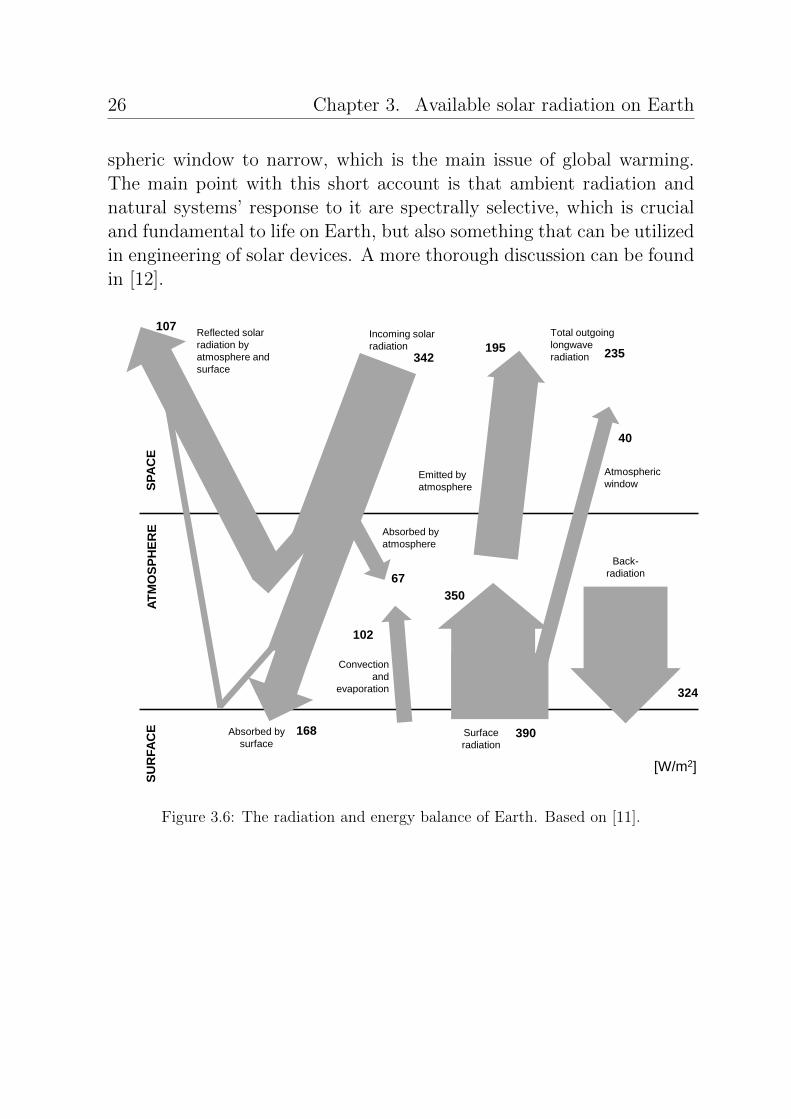
Solar radiation is the most important source of energy on the planet.Other sources include geothermal energy and tidal energy resulting fromthe moon’s gravitational pull, but the flux of solar energy is very highin comparison. Around 130 000 Gtoe (toe = tonnes of oil equivalents)reach Earth every year, while the contribution from geothermal energyfrom Earth’s mantle is 19 Gtoe and from tidal energy 2 Gtoe [8].

An intricate energy balance between incoming and outgoing radiation ismaintained on Earth. Almost one third of the incident solar energy is re-flected back into space, while the rest is absorbed in the atmosphere, byoceans and in inorganic and organic matter on Earth. The absorbed solarenergy drives meteorological and hydrological processes such as winds,waves and ice melting, and it fuels photosynthesis in the biosphere. Thetotal radiation balance is maintained by outgoing long-wave radiationemitted from Earth’s surface. Part of this radiation leaves Earth whilea substantial part is re-radiated back to Earth. This cycle of surfaceradiation and back-radiation by the atmosphere is maintained by thegreenhouse gases. A simplified outline of this complex balance is sum-marized in Figure 3.6.

Atmospheric damping by absorption influences both solar radiation reach-ing Earth and thermal emission from the ground. Most solar energy canbe transmitted to ground level, due to a gap in the atmospheric absorp-tion, with the exception of the UV and IR parts of the solar spectrum,which are strongly damped (cf. Figure 3.2). Thermal radiation is ab-sorbed by the atmosphere, except in the 8-13 µm range. This is theso-called atmospheric window (cf. Figure 3.6), which is the main chan-nel for loss of gained energy from Earth’s surface. Absorption in this partof the spectrum is dominated by CO2 and H2O. Consequently, increasedconcentrations of greenhouse gases in the atmosphere cause the atmo-


spheric window to narrow, which is the main issue of global warming.The main point with this short account is that ambient radiation andnatural systems’ response to it are spectrally selective, which is crucialand fundamental to life on Earth, but also something that can be utilizedin engineering of solar devices. A more thorough discussion can be foundin [12].

Absorbed by

atmosphere

Convection

and

evaporation

Surface

radiation

Back-

radiation

Atmospheric

window Emitted by

atmosphere

Total outgoing

longwave

radiation

Incoming solar

radiation

Reflected solar

radiation by

atmosphere and

surface

107

342 195

40

350

324

390

102

67

Absorbed by

surface

168

235

SP

AC

E

AT

MO

SP

HE

RE

S

UR

FA

CE

[W/m2]

Figure 3.6: The radiation and energy balance of Earth. Based on [11].

Chapter 4. Quantifying available solar energy on planar surfaces 27

Chapter 4

Quantifying available solar energyon planar surfaces

Solar energy systems typically have a receiving surface that collects so-lar radiation, e.g., a PV array or a solar collector. In order to optimizethe orientation of this surface, we must be able to estimate how muchsolar energy differently oriented surfaces collect. This is complex be-cause the Sun is moving across the sky and seldom faces a fixed surfacedirectly, and because the different radiation components (beam, diffuseand ground-reflected) reach the surface from different angles. Varyingweather conditions also make the availability of these different compo-nents differ from one time to another. For a reliable yield calculation, wemust be able to convert commonly available hourly solar radiation dataon the horizontal plane to radiation on a sloped, planar surface.

The aim of the following sections is to provide a mathematical frame-work for converting solar radiation measured on the horizontal plane toradiation on an arbitrarily oriented planar surface. This set of equationsis often used in professional software for simulation and optimization ofsolar thermal or photovoltaic systems based on measured horizontal irra-diance. It is also very useful for understanding the important parametersthat influence collection of solar energy on a surface. These and otherradiation formulae and mathematical models are discussed in more depthin [2].

28 Chapter 4. Quantifying available solar energy on planar surfaces

4.1 Measured solar irradiance data

Determination of solar irradiance on tilted surfaces typically starts frommeasurements in the horizontal plane. Solar radiation is commonly mea-sured by two main classes of instruments: pyrheliometers and pyranome-ters. A pyrheliometer measures solar radiation coming directly from theSun and a small portion of the sky around the Sun at normal incidence.In this device sunlight typically enters through a window to a thermopile(a device that converts heat to electricity). The electrical signal that isgenerated can be recorded and converted into W/m2. The window of thepyrheliometer acts as a filter that only lets through sunlight in the 0.3-3µm range.

The pyranometer measures total hemispherical (diffuse plus beam) solarradiation, usually on the horizontal plane. This means that the devicemust give an unbiased response to radiation from all directions. It con-sists of a thermopile sensor that is horizontally oriented and a glass domethat limits the wavelength range, as in the pyrheliometer. The glass domepreserves the 180◦ view and shields the thermopile from air convection.Schematic illustrations of a pyranometer and a pyrheliometer are shownin Figure 4.1.

Glass dome

ThermopileThermopile

Tube

Glass window

Acceptance angle

(a) (b)

Figure 4.1: A schematic illustration of a pyranometer (a) and a pyrheliometer (b),based on [9] and [10].


While pyrheliometers only measure normal-incidence beam radiation,global or diffuse radiation can be measured with pyranometers. To mea-sure diffuse radiation a shading ring is attached to the pyranometer toblock beam radiation. A correction factor is then used to compensatefor the loss of view. Beam radiation on the horizontal surface can indi-rectly be measured by two pyranometers, one measuring diffuse and onemeasuring global, and then be obtained as the difference between globalradiation and diffuse radiation.

In the following, we will deal with average radiative flux over some periodof time, typically one hour, which is how monitored data are available.This means that the available radiation is integrated over both time andwavelengths. We will denote integrated and averaged radiation by theletter I:

I =1

t2 − t1

∫ t2

t1

G(t)dt. (4.1)

Monitored radiation is available in time series, and the equations beloware all applied one time step at a time. The time t always refers to themidpoint of the monitored time interval:

t =t1 + t2

2. (4.2)

We will assume that we have the beam and diffuse radiation componentsIb and Id on the horizontal plane. From these we want to obtain thebeam, diffuse and ground-reflected radiation components IbT , IdT andIgT on a tilted planar surface. Expressed in global radiation we wish togo from radiation on the horizontal plane:

I = Ib + Id (4.3)

to radiation on the tilted plane:

IT = IbT + IdT + IgT . (4.4)

The basic strategy is to find the incidence angles of radiation on thehorizontal and tilted surfaces, which are used to weight beam radiation,and the view factor of the tilted plane, which determines the incidentisotropic radiation on the tilted plane.


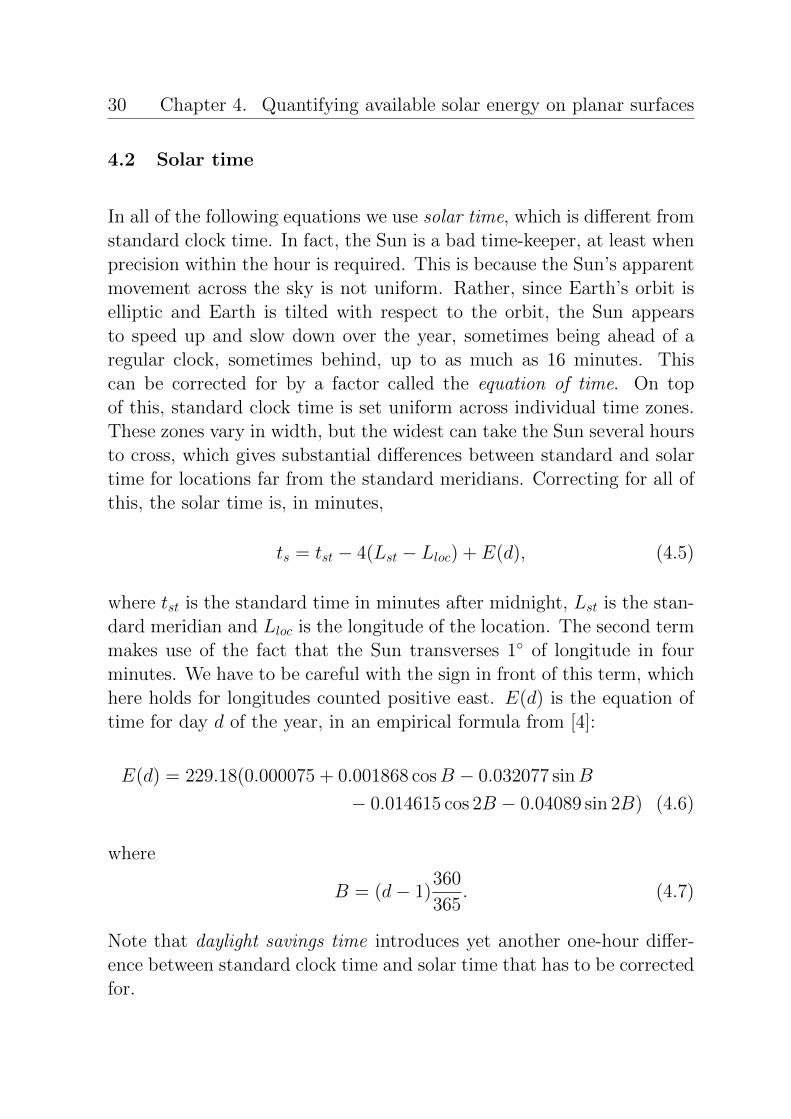
4.2 Solar time

In all of the following equations we use solar time, which is different fromstandard clock time. In fact, the Sun is a bad time-keeper, at least whenprecision within the hour is required. This is because the Sun’s apparentmovement across the sky is not uniform. Rather, since Earth’s orbit iselliptic and Earth is tilted with respect to the orbit, the Sun appearsto speed up and slow down over the year, sometimes being ahead of aregular clock, sometimes behind, up to as much as 16 minutes. Thiscan be corrected for by a factor called the equation of time. On topof this, standard clock time is set uniform across individual time zones.These zones vary in width, but the widest can take the Sun several hoursto cross, which gives substantial differences between standard and solartime for locations far from the standard meridians. Correcting for all ofthis, the solar time is, in minutes,

ts = tst − 4(Lst − Lloc) + E(d), (4.5)

where tst is the standard time in minutes after midnight, Lst is the stan-dard meridian and Lloc is the longitude of the location. The second termmakes use of the fact that the Sun transverses 1◦ of longitude in fourminutes. We have to be careful with the sign in front of this term, whichhere holds for longitudes counted positive east. E(d) is the equation oftime for day d of the year, in an empirical formula from [4]:

E(d) = 229.18(0.000075 + 0.001868 cosB − 0.032077 sinB

− 0.014615 cos 2B − 0.04089 sin 2B) (4.6)

where

B = (d− 1)360

365. (4.7)

Note that daylight savings time introduces yet another one-hour differ-ence between standard clock time and solar time that has to be correctedfor.


4.3 Solar angles

In order to make conversions between horizontal and tilted planes, it isnecessary to know the geometric relationships between the planes andbetween the planes and the Sun at any instant of time. A set of angles,defined below and shown in Figure 4.2, are used to define these relation-ships. First, we have the constant angles defining the orientation andlocation of the tilted plane:

• β, tilt of the plane with respect to the horizontal, 0◦ ≤ β ≤ 180◦

• γ, azimuth angle of the tilted plane, zero due south, west positive,−180◦ ≤ γ ≤ 180◦

• φ, latitude of the location, north positive, −90◦ ≤ φ ≤ 90◦

Second, we have the two time-varying angles that define the position ofthe Sun relative to the celestial sphere1 and Earth:

• δ, declination of the Sun, the ”vertical” position of the Sun on thecelestial sphere, measured in degrees above or below the celestialequator, north positive −23.45◦ ≤ δ ≤ 23.45◦

• ω, hour angle, the angular displacement of the Sun relative to thelocal meridian, zero at noon, afternoon positive, −180◦ ≤ ω ≤ 180◦

The declination makes a complete cycle in one year and can therefore bemodeled with reasonable accuracy as a function of the day of the year d:

δ = 23.45 sin

(360

284 + d

365

). (4.8)

The hour angle, which is the measure of time in the equations, is de-termined from the time of the day. It makes a complete cycle over 24

1The celestial sphere is an imaginary sphere surrounding Earth, on which all celestialobjects are projected. When Earth moves around the Sun, it views the Sun againstthis backdrop of surrounding space. From the viewpoint of Earth, the Sun continuouslytraverses the celestial sphere, making a complete path across it in one year. This pathis called the ecliptic. The celestial equator is the projection of Earth’s equator on thecelestial sphere.


(a)

W

E S

N

γ

θz

β

φ

Lloc

Sun

(b)

ω

δ

Lloc Earth

Sun

Ecliptic

Celestial

equator

23.45°

Figure 4.2: Solar angles used in the calculations. In (a) the angles that define thelocation and orientation of the tilted plane are shown. These are the plane tilt β, theazimuth angle γ and the latitude φ. Also shown are the longitude Lloc and the zenithangle θz. In (b) the angles defining the Sun’s position relative to Earth and the celestialsphere are shown; the declination δ and the hour angle ω.


hours. Since the Sun is displaced 15◦ westward each hour due to rotationof Earth around its own axis and is zero at solar noon, the hour angle is

ω = 15(ts60− 12), (4.9)

where ts is the solar time of the day in minutes.

From these angles, we can find:

• θ, angle of incidence, the angle between the normal to the tiltedplane and the beam radiation on that surface, −180◦ ≤ θ ≤ 180◦.

The angle of incidence is related to all the other angles according to thefollowing equation:

cos θ = sin δ sinφ cos β

− sin δ cosφ sin β cos γ

+ cos δ cosφ cos β cosω

+ cos δ sinφ sin β cos γ cosω

+ cos δ sin β sin γ sinω.

(4.10)

For a horizontal plane, the plane tilt β = 0, and the above relationshipis simplified accordingly. The resulting angle of incidence θz, the zenithangle, which we have already encountered in the discussion on air mass,satisfies

cos θz = cosφ cos δ cosω + sinφ sin δ. (4.11)

For a derivation of these equations for θ and θz, see Appendix A.

4.4 Extraterrestrial radiation

For many radiation calculations it is useful to know the extraterrestrialradiation on the horizontal plane. We have already seen that extraterres-trial radiation with normal incidence can be expressed by Equation 2.7.To obtain the radiation on the horizontal plane, simply multiply by thecosine of the zenith angle:

G0 = Gsc

(1 + 0.033 cos

360d

365

)cos θz. (4.12)


An explanation of why this weighting provides the radiation on the hori-zontal plane is given in Figure 4.3. To obtain the average extraterrestrialradiation in a whole time step we would have to integrate this betweenthe endpoints of the interval. However, as a good approximation we willassume

I0 ≈ G0, (4.13)

which means we pick the instantaneous value for the midpoint of thetime interval.

l

lcos!z

!z

!z

G0n

A B

C

Figure 4.3: Conversion between extraterrestrial radiation with normal incidence andextraterrestrial radiation on the horizontal plane. In the triangle ABC, defined bythe plane perpendicular to the radiation, the horizontal plane and the path of theradiation, the length of side AC is a factor cos θz shorter than the side AB. This holdsalso for sections of the triangle sides defined by parallel rays of radiation (as indicatedby the sections with lengths l and l cos θz). Consequently, the same amount of radiationincident on a unit area on the normal plane will reach an area 1/ cos θz on the horizontalplane, which means the radiation on the horizontal plane is a factor cos θz less intense.Note that this relation holds for all beam radiation and all planes.

4.5 Beam radiation on tilted surfaces

When converting beam radiation between planes we use the geometricfactor Rb, which is defined as the ratio of beam radiation on the tiltedplane to beam radiation on the horizontal plane:

Rb =IbTIb. (4.14)


Following the same reasoning as in Figure 4.3, we find that if Ibn denotesthe beam radiation on a plane perpendicular to the incident radiation,then IbT = Ibn cos θ and Ib = Ibn cos θz, and consequently,

Rb =Ibn cos θ

Ibn cos θz=

cos θ

cos θz. (4.15)

We can then express beam radiation on the tilted plane as

IbT = RbIb (4.16)

An Rb value evaluated at the midpoint of a time interval is used as rep-resentative of the whole interval. As mentioned in [2], this is often agood-enough procedure for hourly values. The conversion is only per-formed when the Sun is above the horizon. Thus, Rb is defined as abovewhen both cos θ > 0 and cos θz > 0, and is zero otherwise. One thing tobe cautious about is the risk of getting unrepresentative values of Rb onintervals involving sunrise and sunset when cos θz is close to zero, whichmay cause highly unrealistic morning or evening radiation peaks.

4.6 Diffuse radiation on tilted surfaces

Now that we can handle beam radiation, we need some similar weightingfor scattered diffuse radiation. If we assume that the diffuse radiationfrom the sky is purely isotropic, this weighting factor is:

fview,sky =1 + cos β

2(4.17)

which is the sky view factor of the surface and describes how much of thesky is visible to the surface. It is easy to see that this expression makessense, noting, e.g., that fview,sky = 1 when the surface is horizontal,fview,sky = 1

2 when it is tilted by 90◦ and fview,sky = 0 when it is facingthe ground. Analogously, the view factor to isotropic radiation from theground can be found as

fview,ground =1− cos β

2. (4.18)


The diffuse radiation component is normally considered to consist ofthree parts – isotropic diffuse, circumsolar diffuse and horizon brighten-ing – which differ in their origin in the sky. The isotropic diffuse partis uniform from every direction, the circumsolar diffuse part is concen-trated around the Sun’s position in the sky and horizon brightening isconcentrated near the horizon. Different models have been formulatedto describe diffuse radiation on the tilted plane. For this compendiumthe so-called Hay and Davies model was chosen. Besides treating partof the diffuse radiation as isotropic, it also models circumsolar radiation.As has been shown in [13], the Hay and Davies model performs similarlyto other, more complex models.

In the Hay and Davies model, diffuse radiation on the tilted surface isexpressed as

IdT = Id

[(1− Ai)

(1 + cos β

2

)+ AiRb

](4.19)

where the anisotropy index Ai is defined as the ratio between the incidentbeam radiation Ib and the extraterrestrial radiation I0 on the horizontalplane:

Ai =IbI0

(4.20)

Thus, since I0 is the incident radiation that would be theoretically pos-sible if there was no atmosphere, Ai is the fraction of radiation that ispreserved as beam radiation after it has passed through the atmosphere.Under clear conditions, Ib approaches I0, causing Ai to be close to 1, andthe diffuse is treated in the same way as beam radiation:

IdT ≈ IdRb. (4.21)

When there is no beam radiation, Ai is zero, and the diffuse radiation isconsidered purely isotropic:

IdT = Id

(1 + cos β

2

)(4.22)

where Id is modified only by the view factor to the sky.


4.7 Ground-reflected radiation

The third and last component of the total radiation on the tilted planeis the radiation reflected from the ground. In reality, numerous objectssuch as buildings, different ground materials, trees, etc., reflect incidentradiation onto the tilted surface. A simplified but standard approach isto assume reflected radiation from one composite source, a horizontal,diffusely reflecting ground. The ground-reflected radiation on the tiltedplane is then dependent only on the reflectance of the ground and theview factor to the ground of the tilted surface:

IgT = Iρg

(1− cos β

2

)(4.23)

where ρg is the ground reflectance and I = Ib + Id is the global radiationon the horizontal plane. The ground reflectance ρg depends on the sur-roundings. At high latitudes, a seasonal variation in ground reflectanceis likely because of snow coverage in the winter.

4.8 Complete model for tilted plane global radiation

The complete model for global radiation on a tilted plane is:

IT = IbT + IdT + IgT . (4.24)

With the formulae for each component in Equations 4.16, 4.22 and 4.23the complete model is:

IT = IbRb + Id

[(1− Ai)

(1 + cos β

2

)+ AiRb

]+

+(Ib + Id)ρg

(1− cos β

2

).

(4.25)

4.9 Some notes on optimization of surface orientation

Some general rules of thumb can be drawn up about how a surface shouldbe tilted to maximize collection of solar radiation over a certain period of


time. Further details can be found, e.g., in [14]. In general, the surfaceshould be oriented so that the incidence angle θ is as close to zero aspossible, as often as possible. Only a two-axis tracking system can keepthe incidence angle at zero at all times. For a fixed surface we have tofind an orientation that is suboptimal on most occasions but as good aspossible over a longer period of time.

The azimuth angle γ should be chosen so that the surface catches the Sunwhen it is at its highest point on the sky. On the northern hemisphere thesurface should be directed south and on the southern hemisphere north.Exceptions include if there is some object shading the Sun (if there isshading in the east, the surface should be oriented west and vice versa),if there are systematic climatic conditions favoring morning or eveningsun or if the collection should match some specific demand profile withpeaks in the morning or evening (which applies mainly to off-grid PVsystems).

The surface tilt β depends on which season the collection is optimizedfor. Summer collection favors lower tilt angles than annual collectionand winter collection requires even higher tilts. For sites within 30◦

of the equator annual energy collection is optimized when the tilt isset roughly equal to the latitude. At higher latitudes lower tilt anglesare more favorable in summer because more energy is available in thesummer than at lower latitudes. A high albedo further favors high tiltangles because it is better with a higher view factor to the ground.

Chapter 5. Exercises 39

Chapter 5

Exercises

Check your understanding

These questions cover the most important concepts. All answers arefound in the sections above.

1. Describe, qualitatively, how the radiation emitted from a black-bodychanges when its temperature increases. How are the total radiationand the wavelength distribution affected?

2. Explain how the Sun’s surface temperature can be determined bymeasuring the flux of solar radiation outside Earth’s atmosphere.

3. What is the solar constant and why does it vary over the year?

4. Which wavelength bands are electromagnetic radiation commonlydivided into? In what way are these wavelength bands relevant insolar engineering?

5. How do the wavelength spectra for extraterrestrial radiation andradiation on Earth’s surface differ? What is the explanation forthese differences?

6. What is the air mass and how can it be approximated?

7. What is the AM1.5 spectrum? Why is it useful in solar engineering?

8. Explain the difference between diffuse and beam radiation. Whydoes solar radiation arrive at Earth’s surface in these two forms?

40 Chapter 5. Exercises

9. What quantities does the Angstrom equation relate?

10. What are the summer and winter solstices and the equinoxes? Howare they related to the Sun’s declination?

11. Describe, for latitudes between the tropics and the polar circles, howthe Sun’s apparent path across the sky changes between the winterand summer solstice.

12. Suggest a setup of measurement devices to monitor beam and diffuseradiation on the horizontal plane.

13. In what ways does solar time differ from local clock time?

14. What is the difference between the angle of incidence and the zenithangle of incidence? Why are these useful when determining thebeam radiation incident on a surface?

15. Explain in a qualitative way what the view factor of a surface is.

16. Describe, qualitatively, how diffuse radiation is handled in the Hayand Davies model when:

(a) The weather is clear.

(b) The sky is completely overcast.

Problems

1. Compare two black-bodies, one with temperature 500 K and onewith temperature 3000 K.

(a) How do they differ in terms of peak wavelength?

(b) How much total radiation is emitted from each of them?

2. A futuristic concept known as a Dyson sphere envisions the entireSun being covered with PV panels. If such a megastructure of panelswas placed around the Sun, covering it entirely, what would be it’stotal power output, given a PV panel efficiency of 15%?


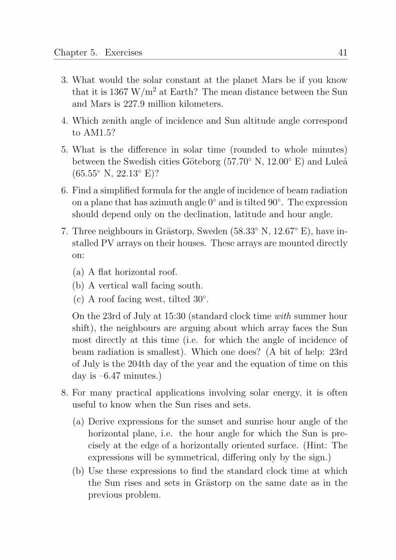
3. What would the solar constant at the planet Mars be if you knowthat it is 1367 W/m2 at Earth? The mean distance between the Sunand Mars is 227.9 million kilometers.

4. Which zenith angle of incidence and Sun altitude angle correspondto AM1.5?

5. What is the difference in solar time (rounded to whole minutes)between the Swedish cities Goteborg (57.70◦ N, 12.00◦ E) and Lulea(65.55◦ N, 22.13◦ E)?

6. Find a simplified formula for the angle of incidence of beam radiationon a plane that has azimuth angle 0◦ and is tilted 90◦. The expressionshould depend only on the declination, latitude and hour angle.

7. Three neighbours in Grastorp, Sweden (58.33◦ N, 12.67◦ E), have in-stalled PV arrays on their houses. These arrays are mounted directlyon:

(a) A flat horizontal roof.

(b) A vertical wall facing south.

(c) A roof facing west, tilted 30◦.

On the 23rd of July at 15:30 (standard clock time with summer hourshift), the neighbours are arguing about which array faces the Sunmost directly at this time (i.e. for which the angle of incidence ofbeam radiation is smallest). Which one does? (A bit of help: 23rdof July is the 204th day of the year and the equation of time on thisday is –6.47 minutes.)

8. For many practical applications involving solar energy, it is oftenuseful to know when the Sun rises and sets.

(a) Derive expressions for the sunset and sunrise hour angle of thehorizontal plane, i.e. the hour angle for which the Sun is pre-cisely at the edge of a horizontally oriented surface. (Hint: Theexpressions will be symmetrical, differing only by the sign.)

(b) Use these expressions to find the standard clock time at whichthe Sun rises and sets in Grastorp on the same date as in theprevious problem.


9. If you know the zenith angle at solar noon, how should you orient asurface to face the Sun directly at this particular time?

10. Consider again the two tilted arrays in Problem 6.

(a) Which are the corresponding geometric factors for beam radia-tion at 15:30 on July 23rd?

(b) Assume that the area of each array is 10 m2. How much beamradiation would these arrays receive if the beam radiation on thehorizontal plane is 500 W/m2 at this time?

11. Find a simplified expression for the zenith incidence angle at solarnoon on the day of the spring or autumn equinox.

12. On a spring day (which happens to be the day of the spring equinox)a group of engineering students have gathered for a picnic at solarnoon in Eslov, Sweden (55.83◦ N, 13.30◦ E). One of them has broughta homebuilt electric stove powered by a PV array, but the othersare unsure if it will be able to collect enough solar energy. At solarnoon on this day, the horizontal plane receives 621 W/m2 of globalradiation, of which 236 W/m2 are diffuse.

(a) It is decided that the PV array is oriented to collect as muchbeam radiation as possible at solar noon. Which tilt and azimuthangles should be chosen?

(b) Assuming that the ground has an albedo of 20%, how much dif-fuse, beam and ground-reflected radiation does the array collectat this orientation? Use the Hay and Davies model for diffuseradiation. Extraterrestrial radiation with normal incidence onthis day is 1376 W/m2.


Answers to problems

1. (a) 5.8 and 0.97 µm, respectively. (b) 3.5 kW/m2 and 4.6 MW/m2.

2. 15% of the total radiative power of the Sun, or 5.79×1025 W. Noticealso that this does not depend on the radius of the Dyson sphere.

3. 588.2 W/m2.

4. Zenith angle 48.2◦, Sun altitude angle 41.8◦.

5. 41 minutes.

6. cos θz = − sin δ cosφ+ cos δ sinφ cosω.

7. Beam radiation on these three arrays has incidence angles (a) 45.4◦,(b) 60.8◦, (c) 58.8◦. Array (a) wins.

8. (a) Sunset hour angle: ω = arccos(− tanφ tan δ), sunrise hour angle:ω = − arccos(− tanφ tan δ). (b) The Sun rises at 03:51 and sets at20:40 (04:51 and 21:40 with summer hour shift). Note that thisresult may differ by several minutes from more detailed calculationsof sunrise and sunset that take into account the angular diameter ofthe Sun and use other, more precise expressions for declination andthe equation of time.

9. γ = 0, β = θz.

10. (a) 0.695 and 0.738, respectively. (b) 3.48 and 3.69 kW per array.

11. θz = φ.

12. (a) γ = 0, β = 55.83◦. (b) GbT = 685 W/m2, GdT = 302 W/m2,GgT = 27.2 W/m2.


Appendix A. Derivation of the incidence angles of beam radiation 45

Appendix A

Derivation of the incidence anglesof beam radiation

A.1 Zenith angle of incidence

The zenith angle θz is the angle between the normal to the horizontalplane at a given location, and the incident beam radiation. The geomet-ric components involved in finding an expression for θz are outlined inFigure A.1. The figure shows the local horizontal plane at some arbitrarylocation on Earth. The plane is defined by its inclination with respect tothe celestial equator, which is the projection of Earth’s equator on thecelestial sphere. The angle between the equator plane and the normalvector of the local plane (v) is equal to the latitude φ of the location.

Over the course of the day, Earth rotates with respect to the celestialsphere, making a complete cycle in one day. This movement is indicatedby the hour angle ω, which is the angle between the position of thecurrent local meridian Lloc of Earth (as projected on the equator plane)and the meridian’s position at solar noon, Lnoon. The Sun’s position onthe celestial sphere is further defined by the declination δ, which is theangular displacement of the Sun from the equator plane. The incidenceangle θz can now be found as the angle between the vector u , whichpoints from the center of the celestial sphere to the Sun’s position, andthe normal vector v of the horizontal plane.

A convenient choice of coordinate system is to have the x axis pointing in

46 Appendix A. Derivation of the incidence angles of beam radiation

δ

ω

φ

Lloc Celestial

equator

Local

horizontal

plane

Lnoon

Sun

u

v

x

y z

θz

Figure A.1: Outline of the geometric relations between the Sun, the celestial equatorand the horizontal plane of Earth at a given location.

the direction of Lloc, the y axis orthogonally to x in the equator plane, andz normal to the equator plane. This makes it possible to directly identifythe components of the vectors u and v from the angles in Figure A.1.Since v by definition is in the xz plane, its components are given solelyby the angle φ as:

v = (cosφ, 0, sinφ)T (A.1)

The vector u is displaced from the xz plane by the angle ω, and by theangle δ from the xy plane, giving the following vector components:

u = (cosω, sinω, tan δ)T , (A.2)

which can be scaled into a unit vector by multiplying with cos δ:

u = (cos δ cosω, cos δ sinω, sin δ)T , (A.3)

Now, since both u and v are unit vectors, the cosine of the angle θzbetween them are given by the dot product:

cos θz = u • v = cosφ cos δ cosω + sinφ sin δ (A.4)

Appendix A. Derivation of the incidence angles of beam radiation 47

A.2 Incidence angle on an arbitrarily oriented plane

The incidence angle of beam radiation on an arbitrarily tilted plane is abit more tricky to derive. Figure A.2 shows how a tilted surface is placedon the horizontal plane of Earth. The orientation of the tilted plane isdefined by the azimuth angle γ and the tilt angle β, defined with respectto the local meridian and the normal of the horizontal plane, respectively.What we now want to find is the angle θ between the Sun vector u andthe normal vector w of the tilted plane.

Celestial

equator

Local

horizontal

plane

v

w

β

ϒ

Tilted

surface

Figure A.2: The geometric relations between the horizontal plane and an arbitrarilyoriented surface.

As Figure A.2 indicates, w can be found by first rotating v around the yaxis by the angle β, then rotating this vector around the original directionof v by the angle γ. A first step, to make this rotation conveniently, isto change the basis of the coordinate system so that x is pointing in thedirection of v while keeping the same y direction. This means that thenew base vectors are:

i = v = (cosφ, 0, sinφ)T

j = (0, 1, 0)T

k = v × j = (− sinφ, 0, cosφ)T

48 Appendix A. Derivation of the incidence angles of beam radiation

The transformation matrix for this operation is:

A =(i j k

)−1=

cosφ 0 sinφ0 1 0

− sinφ 0 cosφ

i.e. a rotation around the y axis by the latitude angle. Applying thistransformation to the Sun vector u we get:

u’ = Au =

cosφ cos δ cosω + sinφ sin δcos δ sinω

− sinφ cos δ cosω + cosφ sin δ

Since the normal vector of the horizontal plane is equal to the new i basevector, we simply have v’ = (1, 0, 0).

Now, to find the normal to the tilted plane, w’ , we rotate v’ an angle βaround the y axis, then an angle γ around the new x axis:

w’ =

1 0 00 cos γ − sin γ0 sin γ cos γ

cos β 0 sin β0 1 0

− sin β 0 cos β

v’ =

cos βsin γ sin β− cos γ sin β

As before, we can now find the cosine of the angle θ as the dot productbetween u’ and w’ :

cos θ = u’ •w’ = sin δ sinφ cos β

− sin δ cosφ sin β cos γ

+ cos δ cosφ cos β cosω

+ cos δ sinφ sin β cos γ cosω

+ cos δ sin β sin γ sinω

Bibliography 49

Bibliography

[1] R. Cohen (2010), Chasing The Sun: The Epic Story of the Star ThatGives Us Life, London, GB: Simon & Schuster.

[2] J.A. Duffie, W.A. Beckman (2006), Solar Engineering of ThermalProcesses, Hoboken, NJ: Wiley.

[3] Solar Spectra, NREL: http://rredc.nrel.gov/solar/spectra/ (2019-04-14).

[4] M. Iqbal (1983), Introduction to Solar Radiation, Toronto: AcademicPress.

[5] M. Sengupta, A. Andreas (2010), Oahu Solar Measure-ment Grid (1-Year Archive): 1-Second Solar Irradiance;Oahu, Hawaii (Data), NREL Report No. DA-5500-56506.http://dx.doi.org/10.5439/1052451

[6] T. Persson (2000), Measurements of Solar Radiation in Sweden 1983-1998, RMK No. 89, Swedish Meteorological and Hydrological Insti-tute (SMHI), Sweden.

[7] A. Angstrom (1928), Recording solar radiation, messages from theSwedish meteorological and hydrological institute, 4:3.

[8] B. Sorensen (2004), Renewable Energy: Its Physics, Engineering, Use,Environmental Impacts, Economy and Planning Aspects, Amster-dam: Elsevier Academic Press.

[9] O. Beckman (1997), Angstrom: Father and Son, Acta UniversitatisUpsaliensis C. Organisation och Historia 60, Uppsala University.

50 Bibliography

[10] M. Paulescu, E. Paulescu, P. Gravila, V. Badescu (2013), Chap-ter 2, Weather Modeling and Forecasting of PV Systems Operation,Springer.

[11] J.T. Kiehl, K.E. Trenberth (1997), Earth’s Annual Global MeanEnergy Budget, Bulletin of the American Meteorological Society 78:197-208.

[12] G.B. Smith, C.G. Granqvist (2011), Green Nanotechnology: Solu-tions for Sustainability and Energy in the Built Environment, BocaRaton, FL: CRC Press.

[13] D.T. Reindl, W.A. Beckman, J.A. Duffie (1990), Evaluation ofhourly tilted surface radiation models, Solar Energy 45: 9-17.

[14] B. Perers (1999), The Solar Resource in Cold Climates, in: M. Ross,J. Royer (Eds.), Photovoltaics in Cold Climates, London: James &James.

Author biographies

Joakim Widen is a Full Professor at the Depart-ment of Engineering Sciences at Uppsala Univer-sity, Sweden, and Chair of the Division of CivilEngineering. His main area of expertise is spatio-temporal modeling of solar irradiance and its ap-plication in energy system operation and urban-scale building modeling.

Joakim Munkhammar is an Associate Professorat the Department of Engineering Sciences at Up-psala University. His research is mainly focusedon solar irradiance variability modeling and fore-casting, as well as applications in energy systemssuch as electric vehicle charging.

Documents

Solar Radiation Theory - DiVA portaluu.diva-portal.org/smash/get/diva2:1305017/FULLTEXT01.pdf2.2 Planck’s radiation law In order to understand the properties of the solar radiation