Embed Size (px)
Citation preview

SOLID MODELING USING IMPLICIT SOLID ELEMENTS
By
JONGHO LEE
A DISSERTATION PRESENTED TO THE GRADUATE SCHOOL OF THE UNIVERSITY OF FLORIDA IN PARTIAL FULFILLMENT
OF THE REQUIREMENTS FOR THE DEGREE OF DOCTOR OF PHILOSOPHY
UNIVERSITY OF FLORIDA
2003

Copyright 2003
by
Jongho Lee

To my lovely family

ACKNOWLEDGMENTS
I would like to express my sincere gratitude to my advisor and the chairman of my
supervisory committee, Dr. Ashok V. Kumar, for his guidance, encouragement and
patience throughout my study. I feel myself very fortunate not only to have benefited
from his academic guidance but also to have enjoyed his invaluable friendship. Without
his assistance this study would never have been completed.
I am also grateful to my committee members, Dr. John C. Ziegert, Dr. John K.
Schueller, Dr. Carl C. Crane and Dr. Baba C. Vemuri, for their advice, comments and
patience in reviewing this dissertation.
I would also like to thank my parents, brothers, my wife, Duyoung Kim, and my
lovely two daughters, Jasmine and Anna, for their valuable love and continuous support
during my study.
iv

TABLE OF CONTENTS Page ACKNOWLEDGMENTS ................................................................................................. iv
LIST OF TABLES........................................................................................................... viii
LIST OF FIGURES ........................................................................................................... ix
ABSTRACT..................................................................................................................... xiii
CHAPTER 1 INTRODUCTION ........................................................................................................1
1.1 Overview.................................................................................................................1 1.2 Goal and Objectives................................................................................................4 1.3 Outline ....................................................................................................................4
2 SOLID REPRESENTATION SCHEMES ...................................................................6
2.1 Geometric Modeling...............................................................................................6 2.2 Constructive Solid Geometry (CSG) ......................................................................7 2.3 Boundary Representation (B-Rep) .......................................................................11 2.4 Hybrid System ......................................................................................................13 2.5 Sweep Features .....................................................................................................14 2.6 Implicit Surfaces or Level Set Surfaces................................................................15
3 IMPLICIT SOLID ELEMENTS ................................................................................17
3.1 Definition of Implicit Solid Elements...................................................................17 3.2 Definition of the Solid within an Implicit Solid Element.....................................20 3.3 3D Hexahedral Solid Elements.............................................................................21 3.4 Defining and Editing Primitives ...........................................................................23 3.5 Defining Complex Geometries using Implicit Solid Elements ............................25 3.6 Heterogeneous Solid Model Capability................................................................26
4 TWO DIMENSIONAL PRIMITIVES.......................................................................28
4.1 2D Primitives by 9-Node Quadrilateral Elements ................................................28 4.2 Mapping in 2D Solid Elements.............................................................................32
v

5 CONSTANT CROSS-SECTION SWEEP.................................................................36
5.1 Extrude Elements..................................................................................................37 5.2 Revolve Elements .................................................................................................40 5.3 Sweep Elements....................................................................................................42
6 VARIABLE CROSS SECTION SWEEP ..................................................................46
6.1 Straight Blend Element.........................................................................................47 6.2 Smooth Blend Element .........................................................................................55 6.3 Sweep Blend .........................................................................................................67
7 CSG REPRESENTATION USING IMPLICIT ELEMENTS ...................................69
7.1 Surface Normal Vectors .....................................................................................69 7.2 Set membership classification within an element...............................................74 7.3 Constructive Solid Geometry using Implicit Solid Elements...............................77
8 VOLUME OF THE SOLID MODEL ........................................................................88
8.1 Linear Approximate Step Function ......................................................................88 8.2 Constructing the Step Function for the CSG Solid...............................................91 8.3 Computing the volume of the solid ......................................................................93
9 ALGORITHM FOR GRAPHICAL DISPLAY........................................................101
9.1 Overview of Computer Graphics........................................................................101 9.2 2D Primitive Display ..........................................................................................102 9.3 2D Boolean Result Display ................................................................................104 9.4 3D Primitive Display ..........................................................................................106 9.5 3D Boolean Result Display ................................................................................108 9.6 Discussions and Suggestion for improvement....................................................116
10 CONCLUSION AND DISCUSSION ......................................................................118
10.1 Conclusion ........................................................................................................118 10.2 Future Work......................................................................................................119
APPENDIX SCENEGRAPH AND CLASS STRUCTURE................................................................120
A.1 SceneGraph Structure for Java3D.....................................................................120 A.2 SDModeler Classes...........................................................................................121 A.3 SDModeler Class Structure ..............................................................................122
vi

LIST OF REFERENCES.................................................................................................125
BIOGRAPHICAL SKETCH ...........................................................................................127
vii

LIST OF TABLES
Table page 3-1. Basis functions for the 9 node quadrilateral element .................................................19
3-2. Hexahedral 8-node basis functions.............................................................................22
3-3. Hexahedral 18-node basis functions...........................................................................22
4-1. Samples of 2D primitive design .................................................................................30
4-2. Analytical solutions for the 4 node quadratic element mapping (parallelogram) ......34
4-3. Analytical solutions for the 4 node quadratic element mapping (non-parallelogram)35
7-1. Surface normal vectors on the boundary of the element ............................................73
8-1. Simple examples for Boolean operation between approximate step functions where f1 and f2 both represent squares....................................................................................90
8-2. Function operator denoted by B where hA and hB are any arbitrary step functions ....93
8-3. Volume integration of Figure 8-6 by changing subdivision number where exact volume is 1.589 (Order of integration = 3, ε =0.001).............................................98
8-4. Volume integration of Figure 8-6 by changing the order of gauss integration where exact volume is 1.589 (Subdivision # = 4, ε =0.001) .............................................99
8-5. Volume integration of Figure 8-6 by changing ε in the linear step function where exact volume is 1.589 (Order of integration = 3, Subdivision # = 4)......................99
8-6. Examples for computing the volume of the solid.......................................................99
viii

LIST OF FIGURES
Figure page 2-1. Example of CSG binary tree structure..........................................................................8
2-2. Comparison between the ordinary Boolean and regularized Boolean operation .........8
2-3. Regularized Boolean treatment in overlapped case......................................................9
2-4. Examples of neighborhood models on the vertices in 2D..........................................10
2-5. Mathematical description of the primitives by half-spaces A) Half-space by x-y plane B) Block by half spaces C) Cylinder by half spaces ......................................11
2-6. Basic concept of B-Rep model ...................................................................................12
2-7. Example of typical B-Rep data structure....................................................................13
3-1. Quadrilateral 9-node element in two different coordinate systems A) Parametric space (r, s coordinates) B) Real space (x, y : Global coordinates)..........................18
3-2. Density distribution within a 9 node quadratic element A) Density fringes B) Density contours C) Density Plot ..........................................................................................20
3-3. Solids defined using 3D hexahedral elements A) 8 Node element B) 18 Node element .....................................................................................................................23
3-4. Editing the face represented using 2D element ..........................................................24
3-5. Three ways of editing solids represented using 3D element ......................................25
3-6. Implicit representation of planar face using shape density function A) Density Grid B) Contours of density function ...............................................................................25
3-7. 3D Composition Destribution A) 8-node element B) 18-node element.....................27
4-1. 2D primitive examples A) Rectangle B) Circle C) Ellipse ........................................28
4-2. Constructing a 2D primitive by the part of an existing shape ....................................31
4-3. 2D primitives and its nodal density distribution A) Quarter circle B) Semi circle C) Triangle D) Wedge shape.........................................................................................31
ix

5-1. 2D primitive element and the corresponding extrude element...................................37
5-2. Solid created by extruding ellipse ..............................................................................39
5-3. Extrusion of profile defined using multiple elements ................................................40
5-4.. Cylindrical coordinate system for revolving .............................................................40
5-5. Mapping from cylindrical to Cartesian coordinates ...................................................41
5-6. Examples for revolved solids .....................................................................................42
5-7. Relationship between the global and local coordinate systems..................................43
5-8. Examples of solids created using sweep elements .....................................................45
6-1. Two neighboring straight blend elements having quadrateral 9 node elements as 2D profile .......................................................................................................................49
6-2. A straight blend element having quadratic 9 node elements as 2D profiles...............50
6-3. Cross section at a certain t* in the straight blend element ..........................................52
6-4. Examples of straight blend using blend elements ......................................................55
6-5. Two neighboring smooth blend elements having quadratic 9 node elements as 2D profile .......................................................................................................................57
6-6. A smooth blend element having quadratic 9 node elements as 2D profile ................60
6-7. Cross section at a certain t* in smooth blend elements ..............................................62
6-8. Examples of Smooth blend using blend elements ......................................................67
7-1. Flow chart for set-membership classification in an individual solid element ............76
7-2. CSG tree data structure...............................................................................................77
7-3. 2D Boolean operation in CSG....................................................................................78
7-4. 3D Constructive Solid Geometry Tree .......................................................................79
7-5. surface normal vectors and corresponding triangles ..................................................82
7-6. Constructing a triangle from one normal vector.........................................................82
7-7. Constructing two triangles from two normal vectors .................................................83
7-8. Constructing three triangles from three normal vectors .............................................84
x

7-9. Neighborhood model using graphical method............................................................86
8-1. Linear approximate step function graph.....................................................................88
8-2. Transform from the implicit surface function to its linear approximate step function89
8-3. Implicit surfaces defining a solid within an element in the parametric space A) 2D solid element B) 3D solid element ...........................................................................91
8-4. Labeling CSG tree nodes for constructing the approximate step-function ................92
8-5. Subdivision of the 2D element and subdividing method A) Quadtree subdivision in a 2D element B) An example of quadtree representation structure C) An example of octree representation structure .................................................................................95
8-6. A simple 2D example used for comparing the numerical integration results by changing some parameters such as subdivision number, order of integration and ε ...............................................................................................................................98
9-1. Graphics of a curve...................................................................................................101
9-2. Graphics of a sphere and its triangulation ................................................................102
9-3. Ray methods for finding points on the boundary of the solid in 2D ........................103
9-4. Computing the points on the boundary of the ellipse...............................................104
9-5. Union of two squares in 2D......................................................................................105
9-6. Bounding box for a 2D solid element.......................................................................106
9-7. Computing the points on the boundary of the solid A) 2D profile to be swept B) Points on the extrude C) Points on the revolve D) Points on the sweep ................107
9-8. Finding the points on the boundary of the varying cross section sweep ..................108
9-9. 3D CSG tree structure...............................................................................................110
9-10. All triangleArrays composing the base and dependent solid .................................111
9-11. Bounding cylinder method between two elements.................................................112
9-12. All triangleArrays relevant to intersected elements ...............................................112
9-13. Triangle-Triangle intersection A) Plane-Edge intersection B) Edge-Edge intersection .............................................................................................................113
9-14. TriangleArrays having actually intersected triangles .............................................113
xi

9-15. Mapping the triangle in space onto the local u-v plane..........................................114
9-16. Subdivided triangles after Delaunay triangulation .................................................115
9-17. Flow chart for constructing the graphics for the 3D Boolean result ......................116
A-1. SceneGraph structure for the solid modeler using implicit solid elements .............120
A-2. Class structure for the solid modeler using implicit solid elements ........................122
A-3. ShapeDensity class structure ...................................................................................123
A-4. InteractiveCommand class structure........................................................................123
A-5. CommandList class structure...................................................................................124
A-6. PositionConstraint class structure............................................................................124
xii

Abstract of Dissertation Presented to the Graduate School of the University of Florida in Partial Fulfillment of the Requirements for the Degree of Doctor of Philosophy
SOLID MODELING USING IMPLICIT SOLID ELEMENTS
By
Jongho Lee
August 2003
Chair: Ashok V. Kumar Major Department: Mechanical and Aerospace Engineering
A solid modeling technique using implicit surface representation is presented
where the implicit surface function (referred to here as density function) is defined by
piece-wise interpolation within quadrilateral elements in 2D and hexahedral elements in
3D. Within each element the density function is defined as a parametric function. The
solid is defined as the region within the element where the density is greater than a
threshold or “level set” value. The boundary of the solid is therefore a contour of the
density function along which the density is equal to the level set value or the boundary of
the element where the density is greater than the level set value. Simple shapes or
primitives can often be defined using a single implicit solid element while more complex
geometry can be represented either using a grid/mesh of elements or by Boolean
combination of simple primitives. The geometry of the primitives can be edited or
modified by changing the density values at the nodes of the elements, by changing the
size of the element as well as by changing the level set value. In this study, hexahedral
xiii

elements are presented along with basis functions that can be used to represent primitive
solids created by sweeping 2D geometry along trajectories that can be lines, arcs or
arbitrary parametric curves. In traditional solid modeling software based on the B-Rep
(boundary representation) approach, solid primitives are often created by sweep
operations. The elements described in this study enable the representation of such solids
using implicit surfaces. This primitive representation scheme is axes independent because
the implicit function representing the solid is defined as a parametric function within
quadrilateral or hexahedral elements while general implicit surface functions are axes
dependent. In general it is easier to determine whether a given point is inside, outside or
on the boundary of a solid if the boundary is represented using implicit equations. Since it
is necessary to repeatedly classify points in this manner for many graphical display and
volumetric property evaluation algorithms implicit representation is particularly suited
for representing primitives in a CSG tree. For the implicit solid element representation, it
is also necessary to first map from global coordinates to parametric coordinates to
perform this classification. This mapping is shown to be easy to perform if the elements
have parallel edges and faces. The volume of the solid can be computed by defining the
linear approximate step function, which has a unit value almost everywhere in the interior
of the solid and zero in exterior of the solid. This linear approximate step function can be
numerically integrated to compute the volume.
xiv

CHAPTER 1 INTRODUCTION
1.1 Overview
Solid modeling is the fundamental technology on which CAD/CAM/CAE
(Computer Aided Design/Manufacturing/Engineering) systems have been built. Solid
modeling technique (sometimes called volumetric modeling) has been used for many
applications including visualization, geometry design, assembly verification, engineering
analysis and generating NC machining codes. The use of solid models for design and
manufacturing is becoming more widespread with the increasing availability of computer
technology.
Solid models enable one to construct unambiguous models of three-dimensional
objects. Such unambiguous models are necessary to construct algorithms for
automatically computing volumetric properties such as surface area and volume of the
solid. Algorithms for automatic generation finite element mesh for engineering analysis
also depend on the ability to construct precise, unambiguous models of solids.
Algorithms have also been developed to generate tool paths for machining given the solid
model of the part to be machined. More recently developed fabrication and prototyping
technology called the layered-manufacturing technique (also known as rapid prototyping
or the solid freeform fabrication technique) also need solid models of the part to be
constructed.
The most popular schemes in current solid modeling are Boundary Representation
(or B-Rep) and Constructive Solid Geometry (CSG). In B-Rep, a solid is represented by
1

2
the boundary information of the solid where vertices, edges and faces (geometry
information) are saved together with the information on how they are connected to build
the boundary of the solid (topology information). The geometry of the boundaries are
represented using parametric equations of the form X(u) or X(u,v) where X is a position
vector of a point on the curve or surface. In CSG representation, Boolean operations
applied on primitives that are simple shapes such as a block, cylinder, sphere or cone are
saved in the binary tree data structure where primitives are defined by Boolean
combination of half-spaces. Half spaces are implicit equations of curves or surfaces that
are represented as f(x,y) ≥ 0 (curves) or f(x,y,z) ≥ 0 (surfaces).
Current commercial solid modeling systems typically use a hybrid system where
the solid is constructed by the Boolean combination of primitives that are represented
using B-Rep models. The B-Rep model of the resultant solid is automatically constructed
from the CSG tree using algorithms known as Boundary evaluation.
In almost all current solid modeling systems, a feature based approach is provided
as the user interface for creating solids where primitives are constructed by sweeping 2D
profiles along a trajectory. Such sweep features for creating 3D primitives are popular
because it enables the user to create primitives interactively. B-Rep solid models use
parametric equations for geometric components such as lines, curves and surfaces.
Creating B-Rep primitives by sweep operations is simple and straight forward because it
is easy to define the equations of surfaces created by sweeping a curve along a trajectory
in the parametric form. However, it is difficult to construct such sweep primitives by a
Boolean combination of half-spaces as is done in traditional CSG systems.

3
Solid modeling systems based on B-Rep models is very difficult and expensive to
implement. The main reason for the difficulty is that the B-Rep model for the resultant
geometry has to be constructed automatically from B-Rep models of the primitives using
the information about the Boolean operations used to combine them. For each regularized
Boolean operation, the boundary evaluator algorithm, detects intersections between
participating solids, computes intersection geometries (intersection points and curves as
well as sub-divided faces) and classifies them according to whether the geometry is in, on
or outside the final solid defined by the Boolean operation. As mentioned earlier, B-Rep
models need topology information as well as geometric information. Constructing
connectivity (topology) between geometric components automatically is very difficult to
be performed for complex geometries. And it is also very expensive to classify a given
point, curve or face as being inside, outside or on the solid. The procedure for such
classification is called set-membership classification.
In traditional CSG models, the topology of the solid is not explicitly represented.
Therefore, there is no need for Boundary evaluation algorithms. An algorithm is needed
to generate the graphics of the resultant solid using the information available in the CSG
tree. Even though in general the graphics image is difficult to generate for implicit curves
and surfaces, the implementation of a CSG solid modeling system is easier because there
is no need for Boundary evaluation algorithms. However, in order for such a modeling
system to be useful it is necessary that a feature based modeling interface can be
constructed. No attempt has been made to construct sweep features using implicit curves
and surfaces since all current solid modeling systems use B-Rep models. Therefore one

4
of the motivations of this study is to develop a feature based solid modeling system
where all the boundaries of the solid are represented using implicit equations.
1.2 Goal and Objectives
The goal of this research is to study the feasibility, advantages, and disadvantages
of building a feature based solid modeling system that uses only implicit equations for
curves and surfaces as it is done in traditional CSG solid modeling systems. Such solid
models in this thesis are referred as implicit solid models. In order to develop such a
system, implicit solid elements that are quadrilateral and hexahedral elements used to
represent implicit curves and surfaces respectively have been used. The main objectives
of the thesis are listed below.
1. Develop quadrilateral implicit solid elements to represents simple 2D primitives such as circles, ellipses, rectangles and triangles.
2. Develop hexahedral implicit solid elements to represent solid primitives obtained by extruding, revolving or sweeping 2D primitives defined using quadrilateral implicit solid elements.
3. Develop hexahedral implicit solid elements to represent a solid primitive obtained by blending between two or more different 2D primitives
4. Construct algorithms for displaying solids created by Boolean combinations of primitives represented using implicit solid elements.
5. Construct algorithms for automatically computing volumetric properties. 1.3 Outline
In Chapter 2, current popular solid modeling techniques are introduced to give an
overview for the reader. In Chapter 3, the definition of implicit solid elements is
described and in Chapter 4, simple 2D primitives using 2D implicit solid elements are
introduced. In Chapters 5 and 6, constant cross-section sweep elements and variable
cross-section sweep elements are described respectively. Algorithms for set membership
classification at a given point with respect to a primitive and a solid represented by a
CSG tree structures are described in Chapter 7. In Chapter 8, the method to compute the

5
volume of the solid is presented and in Chapter 9, issues associated with generating the
computer graphics of the solid are described. Finally, Chapter 10 provides conclusions
and discussions.

CHAPTER 2 SOLID REPRESENTATION SCHEMES
2.1 Geometric Modeling
Geometric Modeling systems are used in the design process for visualization,
assembly verification, engineering analysis, generating NC machining codes, etc. It often
eliminates the need for making many physical prototypes to test design concepts. There
are three different types of geometric modeling systems: wireframe modeling, surface
modeling and solid modeling.
Wireframe Modeling is the earliest method, where a shape is represented by its
characteristic lines and points. Although it has some advantages such as simple user
inputs and ease of implementation, the following two disadvantages make this
representation unpopular. First, the shapes represented only by lines and points are very
ambiguous. Second, there is no information about the inside and outside boundary
surfaces of the object. Therefore it cannot be used for mass property computation, tool
path generation or finite element analysis.
Surface Modeling has surface information in addition to the wireframe model
information. Therefore, the tool path for the NC machines can be generated for the
surfaces. However, since it also does not have information to distinguish between the
inside and the outside of the object, Boolean operations cannot be used to combine such
models and it is difficult or impossible to construct other algorithms for automatically
manipulating such models as an example when generating a mesh.
6

7
Solid Modeling was introduced to overcome some of the limitations of the other
schemes mentioned above. Solid modeling techniques began to develop in the late 1960s
and early 1970s. The fundamental concepts and definitions of solid modeling are well
introduced in many books [Hoffmann, 1987, Zeid, 1991., Mortenson, 1997., Lee, 1999].
The most popular schemes in current solid modeling are Boundary Representation (or B-
Rep) and Constructive Solid Geometry (CSG). In B-Rep, a solid is represented by the
boundary information of the solid where vertices, edges, and faces are saved together
with the information on how they are connected to build the boundary of the solid. In
CSG representation, Boolean operations applied on primitives are saved in the binary tree
data structure. These two representation schemes are described in the following section.
2.2 Constructive Solid Geometry (CSG)
The constructive solid geometry representation technique defines complex solids as
Boolean combinations of simpler solids called primitives. A Boolean operation is one of
the best methods to create complex solids. It dramatically increases the repertoires of the
shapes to be modeled. A binary tree data structure is used to save the Boolean operations
between primitives. The following is an example of CSG tree data structure, where the
final solid is generated by the union of the primitive A and B, followed by the difference
of the primitive C.
In this tree structure, leaf nodes (or primitive nodes) represent primitive solids and
branch nodes have Boolean types such as union, difference, and intersect. Boolean
operations can be explained by set theory. However, the set theory applied here is
different from the original set theory. A modified Boolean operation has been defined for
solid modeling which is referred to as Regularized Boolean operation, where the Boolean
combination results between primitives are closed and dimensionally homogeneous.

8
CU
A B
Figure 2-1. Example of CSG binary tree structure
The following example shows how the regularized Boolean operation is different
from the original Boolean operation. Regularized Boolean operations are denoted by ∪*,
∩*, and −* respectively while the ordinary Boolean operations are denoted by ∪, ∩, and
−.
Union Intersection Difference
∪ ∪* ∩ ∩* − −*
B
A
B
A
Figure 2-2. Comparison between the ordinary Boolean and regularized Boolean operation
As shown in Figure 2-2, problems always occur when the boundaries of the
primitives overlap. These special cases can be treated to create a regularized result by
comparing the directions of both boundary normal vectors. For example, in the
regularized intersection, if both boundary normal vectors have the same direction, the

9
boundary is also the boundary of the regularized Boolean combination. On the contrary,
if they have opposite directions, it should be removed to construct the regularized
Boolean combination. The following shows all-special cases, where nA and nB are the
boundary normal vectors of the primitive A and B at the overlapped part respectively.
∪* ON IN ∩* ON OUT −* OUT ON
BnB
A nA
B A nB
nA
Figure 2-3. Regularized Boolean treatment in overlapped case
The method using normal vectors for the regularized Boolean combination in solid
modeling cannot be used when multiple normal vectors are involved. For instance
vertices in 2D or 3D and edges in 3D cannot be simply classified as in, out or on the solid
because those have multiple normal vectors. This problem can be solved by using a
neighborhood model where points close to the given point (or in its neighborhood) are
examined. Figure 2-4 shows an example of a neighborhood model where a small disk
symbolizes the neighborhood, and the shaded area indicates points inside the solid. The
neighborhood model at a point for the Boolean result is constructed by applying the
Boolean operation to the neighborhood models at the point for the two participating
solids.

10
Figure 2-4. Examples of neighborhood models on the vertices in 2D
AB
A
B
B
A
On
On
AUB
AUB
There are three important subsets defined by a solid, where the solid is considered a
set of points. Those are the set of interior points, points on the boundary of the solid, and
all points outside the solid. Set-membership classification of a point involves assigning
the point to one of these sets. It is an essential step to do a Boolean operation.
Primitives are simple shapes such as a block, cylinder, sphere or cone, where the
mathematical descriptions of the primitives are defined by the intersection of a set of
curved or planar half-spaces. A half space divides the space into two regions, for
instance, an infinite x-y plane divides the space into the region of z>0 and the region of
z<0 as shown in Figure 2-5A. Figure 2-5B and Figure 2-5C show how to define the
primitive block and cylinder by half-spaces respectively. Where the block is represented
by the intersection of six planar half-spaces and the cylinder is represented by the
intersection of a cylindrical half-space and two planar half-spaces.

11
ax ≥
by ≥
ez ≥
az ≥
bz ≤
z
z>0
z
y z<0 x
(A) (B) (C)
Figure 2-5. Mathematical description of the primitives by half-spaces A) Half-space by x-y plane B) Block by half spaces C) Cylinder by half spaces
Arrows indicate the direction of the material. The detailed mathematical
descriptions can be represented as follows:
Block : , bxa ≤≤ dyc ≤≤ , fze ≤≤
Cylinder : 0 , 222 ryx ≤+≤ bza ≤≤
This kind of description is good for set membership classification because the sign
of the implicit function representing the half space can be used to classify the point. CSG
representation does not include topology information and therefore additional
computation is necessary to determine the connectivity between boundary entities. Such
connectivity information is used in many applications such as mesh generation and tool
path generation for machining.
2.3 Boundary Representation (B-Rep)
The B-Rep model of a solid consists of parametric equations of the vertices, edges
and faces of the solid together with the connectivity information between them. The
geometry information in a B-Rep model is composed of surface equations, curve

12
equations, and point coordinates. The connectivity between the geometric entities is the
topology information which is the interrelationship among faces, edges and vertices.
It is based on the idea that the boundary of a solid consists of faces (surfaces)
bounded by edges (curves), which in turn are bounded, by vertices (points). In B-Rep, a
face is a subset or limited region of some more extensive surface. For example, planar
faces are subsets of infinite planes that are bounded by edges, while curved faces are
represented as parametric surfaces bounded by edges. Thus, these equations are saved in
the B-Rep data structure. The topology information is represented as relations between
faces, edges, and vertices. In Figure 2-6, the face F1 is composed of four edges (E1, E2,
E4, E3) and each edge is represented by two vertices. E1 V1V2 F3
F1F1 E2 E4 F2
V4V3 E3
Figure 2-6. Basic concept of B-Rep model
An array of faces, edges, and vertices can be used to represent this kind of simple
polyhedral model. Figure 2-7 shows the typical data structure [Spatial Technology Inc.,
1995] used to represent B-Rep models which consists of shells, faces, loops, half
edges(or coedges), and vertexes.
Figure 2-7 shows classes used to represent the solid model. A solid is denoted as a
BODY which consists of one or more LUMPs. A LUMP is a connected 3D region whose
boundaries are represented using closed SHELLs. A closed SHELL consist of a list of
faces forming a closed volume. As mentioned earlier, the geometry of a face is defined
by a parametric surface equation and is bounded by LOOPs that define its external and
internal boundaries. Loops are defined as a list of half-edges (COEDGEs), which are

13
edges with a direction. Half edges are connected together to form loops such that the
direction of the loop is counter clockwise for the external boundary and clockwise for
internal boundaries when the face is viewed from the outside. Assigning directions to
loops in this manner assists in determining whether a given point is inside, on, or outside
the solid. If the solid has a lot of faces, this kind of set membership classification is
difficult and it requires significant computation. Since every entity is interconnected with
other entities, changing the topology is very complicated in the B-Rep model approach.
F1
V1
E1
C5
C1
V2
L1
L2
Ex )
E1 V1, V2
C1 E1
L1 C1, C2, C3, C4
F1 L1, L2
S1 F1, F2, ….., F10
Lump1 S1
next previous
next
next
POINT
CURVE
SURFACE
VERTEX
EDGE
COEDGE
LOOP
FACE
SHELL
LUMP
BODY
Figure 2-7. Example of typical B-Rep data structure
2.4 Hybrid System
Creating B-Rep models directly by defining each vertex, edge, and surface is
extremely cumbersome. Therefore, hybrid systems were developed where the solid is
represented procedurally using a CSG tree but the primitives are represented using B-
Rep. The B-Rep model of the solid represented by the CSG tree is evaluated

14
automatically using “Boundary Evaluator” algorithms [Requicha and Voelcker, 1985].
For each regularized Boolean operation, the boundary evaluator algorithm, detects
intersections between participating solids, computes intersection geometries (intersection
points and curves as well as sub-divided faces) and classifies them using set membership
classification algorithms to determine whether the geometry is in, on, or outside the final
solid defined by the Boolean operation. While set membership classification is easy when
the solid is represented as a combination of half spaces (where the surfaces are implicit
equations, f(x,y,z) = 0), it is more difficult to do for B-Reps. Furthermore, constructing
the topology of the resultant solid automatically is also difficult. As a result it is very
expensive to build robust and reliable software that can handle every special case.
However, over the years many commercial systems have been developed that have very
reliable boundary evaluator algorithms that are robust and can handle almost all special
and degenerate cases including non-manifold topologies. To cope with the high cost of
implementing these algorithms, many companies in the CAD industry buy “geometric
modeling kernels” from other companies that have already implemented them [Spatial
Technology Inc., 1995].
2.5 Sweep Features
A sweep feature is defined by sweeping a planar shape along an arbitrary space
curve referred to as a sweep trajectory, where the cross section of the sweep solid can be
either constant or varying. This is a very popular and useful method due to the fact that
the solid represented by sweeping is simple to understand and execute. If the sweep
trajectory is a straight line, it is called as translational sweep (or extruded solid). When
the sweep trajectory is a circular arc, it is termed a rotational sweep (or revolved solid).
When the sweep trajectory is an arbitrary parametric curve, it is referred to as a general

15
sweep. Recent research related to sweeping includes three-dimensional object sweeping
and sweep surface representation using coordinate transforms and blending [Martin and
Stephenson, 1990, Choi and Lee, 1990].
2.6 Implicit Surfaces or Level Set Surfaces
Traditionally, implicit curves and surfaces are represented as f(x) = c where 2R∈x
for planar curves and for surfaces. They are sometimes referred to as level sets or
iso-curve/surface since the curve or surface corresponds to a constant value of the
function f(x). If c = 0 then the curve or surface is called the zero set of f(x). An implicit
surface divides space into regions where f(x) > 0 and f(x) < 0. Therefore, if the
boundaries of the solid are represented implicitly as half-spaces one can use the sign of
f(x) to perform set membership classification that is to determine whether a given point is
inside, outside, or on the solid. Despite this advantage, implicit representation for curves
and surfaces has traditionally been considered inferior to parametric representation. The
reasons suggested for this include axis dependence of implicit curves, difficulty in tracing
or generating graphics, as well as difficulty in fitting and manipulating freeform shapes.
Considerable progress has been made to solve some of these problems due to which
implicit curves and surfaces now have numerous applications in graphics and animation
[Bloomenthal et al., 1997].
3R∈x
To enable graphical display a variety of polygonization, tessellation, or tracing
algorithms have been developed [Wyvill and Overveld, 1997., Lorensen and Cline,
1987]. Ray tracing algorithms have also been used for visualization of implicit surfaces
[Glassener, 1989]. When the implicit function f(x) is a polynomial, the surface is called
an algebraic surface. Most common primitive shapes such as sphere, ellipse, cone, and

16
cylinders can be expressed as algebraic surfaces using quadratic polynomials. For more
complex shapes, implicit algebraic surface patches (or A-splines) have been developed
[Bajaj et al., 1995]. These patches can be used for C1 and C2 interpolations or
approximations and also for interactive free-form modeling schemes. Implicit curves and
surfaces have also been used for visualization problems such as shape reconstruction
from unorganized data sets [Zhao et al., 2000] and dynamic fluid flow [Osher and
Redkiw, 2003]. Recently, R-functions [Shapiro, 1998] have been used to define implicit
solids. The sign of an R-function depends only on the sign of its arguments and not its
magnitude. This property of R-functions can be used to construct implicit functions for
representing solids created by a Boolean combination of implicit surfaces. Furthermore,
the advantage using geometry represented using implicit curves and surfaces in solving
boundary and initial value problems with time varying geometries and boundary
conditions has also been illustrated [Shapiro and Tsukanov, 1999].
Implicit surfaces are often used in computer graphics for representing soft or
deformable objects such as humans, animals, and amorphous blobs. Sometimes, an
implicit surface can be represented by the distance relationship between the surface and a
given basic structure such as point, line, and circle. This kind of method is called distance
metrics or the skeleton method [Tigges and Wyvill, 1999].

CHAPTER 3 IMPLICIT SOLID ELEMENTS
3.1 Definition of Implicit Solid Elements
The implicit curves and surfaces are represented here as the level set of an implicit
surface function φ(r,s) = φb for planar faces or φ(r,s,t) = φb for solids. The implicit
surface function, φ, has been referred to in this study as the shape density function (or
simply density function) [Kumar and Gossard, 1996]. The density function has a value
greater than a threshold or level set value, φb, inside the solid and less than φb outside the
solid. Unlike the traditional approach, where the implicit surface function is defined
directly in terms of the x, y, z or Cartesian coordinates, the density function used here is a
parametric function whose arguments are the parametric coordinates of an implicit solid
element. This is illustrated using a two dimensional example in Figure 3-1 where the
element has nine nodes and its geometry in the parametric space is shown in Figure 3-1A
while its real geometry is shown in Figure 3-1B. In the parametric space the element is a
square whereas in the real space the element can be a distorted quadrilateral. The
mapping between the parametric coordinates and the real coordinates x, y and z is defined
as,
n
i ii 1n
i ii 1n
i ii 1
x(r,s, t) x M (r,s, t),
y(r,s, t) y M (r,s, t) and
z(r,s, t) z M (r,s, t)
=
=
=
=
=
=
∑
∑
∑ (3-1)
17

18
In Eq. 3-1. (xi, yi, zi) are the coordinates of the node i, are mapping basis
functions that define the mapping between the parametric space (r,s,t) and the real space
(x,y,z) and n is the total number of nodes per element. (x,y,z) and n is the total number of nodes per element.
iM (r,s, t)
(A) (A) (B) (B)
5
φ = φb9
1
8
4
3 7
6
2
y
x
9
1
8
3 7 4
6
5 2
s
r
Figure 3-1. Quadrilateral 9-node element in two different coordinate systems A) Parametric space (r, s coordinates) B) Real space (x, y : Global coordinates)
Figure 3-1. Quadrilateral 9-node element in two different coordinate systems A) Parametric space (r, s coordinates) B) Real space (x, y : Global coordinates)
The density functions are defined within the elements by specifying the values of
the functions at the nodes of these elements. The value of the function within each
element is obtained by interpolating the values at the nodes using appropriate basis
functions or interpolation functions. A parametric interpolation scheme is used as shown
below where parameters (r, s, t) vary between –1 and 1.
∑=
=n
iii srNsr
1),(),( φφ ∑
=
=n
iii srNsr
1),(),( φφ for 2D elements (3-2) for 2D elements (3-2)
∑=
=n
iii tsrNtsr
1),,(),,( φφ ∑
=
=n
iii tsrNtsr
1),,(),,( φφ for 3D elements (3-3) for 3D elements (3-3)
Where, φi is the density at the node i, Ni is the interpolation basis function at the
node i used to interpolate the density, and n is the total number of nodes in the element.
Each element is a cube (or square in 2D) of side length equal to 2 in the parametric space
since the parameters r, s and t vary from -1 to 1 within each element. If the mapping basis
functions are identical to the density interpolation basis functions
Where, φ
iM (r,s, t)iM (r,s, t) iN (r,s, t)iN (r,s, t)
i is the density at the node i, Ni is the interpolation basis function at the
node i used to interpolate the density, and n is the total number of nodes in the element.
Each element is a cube (or square in 2D) of side length equal to 2 in the parametric space
since the parameters r, s and t vary from -1 to 1 within each element. If the mapping basis
functions are identical to the density interpolation basis functions

19
then the element can be referred to as “iso-parametric element”. However, it is often
beneficial to use simpler basis functions for the mapping.
In this formulation, even though the boundary of the solid is represented in the
implicit form φ(x,y,z) = φb, the density function itself is represented in a parametric form,
φ(r, s, t) with a mapping defined between the parameters (r,s,t) and the global coordinates
(x,y,z). Therefore, many of the advantages traditionally associated with parametric curves
and surfaces are also applicable to the implicit solid element approach including axes
independence and the ease in tracing. The parametric form of the density function enables
the development of simple algorithms to polygonize the surface for graphical display.
The detailed description for one way of graphical display used in this system is explained
in Chapter 9.
The following table shows the basis functions for the 9 node quadrilateral element
where the numbering system is as shown in Figure 3-1.
Table 3-1 Basis functions for the 9 node quadrilateral element N1 = 0.25(r2+r)(s2+s) N2 = 0.25(r2-r)(s2+s) N3 = 0.25(r2-r)(s2-s) N4 = 0.25(r2+r)(s2-s) N5 = 0.5(1-r2)(s2+s) N6 = 0.5(r2-r)(1-s2) N7 = 0.5(1-r2)(s2-s) N8 =0.5(r2+r)(1-s2) N9 = (1-r2)(1-s2)
These shape functions are derived by Lagrange interpolation such that Ni is, equal
to 1 at node i and is zero at other nodes. For instance, N1 = 0 at node 2 to 9 is equivalent
to requiring that N1 = 0 along edges r = 0, r = -1, s = 0 and s = -1. Therefore N1 can be
represented by
N1 = c(r2+r)(s2+s) where c is some constant that is determined from the condition N1 = 1 at node 1.
Since r = 1 and s =1 at node 1, yields

20
1 = c(12+1)(12+1)= 4c Which yields c = 0.25.
Similarly other shape functions at nodes 2 to 9 are derived as shown in Table 3-1.
Figure 3-2 shows the density distribution within a 9-node element when the density
at the corner nodes are set equal to 0, the density at mid-edge nodes are set to 0.5 and the
density is 1 at the center node.
(A)
-1 -0.8 -0.6 -0.4 -0.2 0 0.2 0.4 0.6 0.8 1
-1
-0.8
-0.6
-0.4
-0.2
0
0.2
0.4
0.6
0.8
1
r
s
0.4
0.4
0.5
0.5
0.50.5
0.5
0.6
0.6
0.6
0.6
0.60.6
0.6
0.6
0.7 0.70.7
0.7
0.7
0.7
0.8
0.8
0.80.8
0.8
0.9
0.9
0.9
0.9
(B)
(C)
Figure 3-2 Density distribution within a 9 node quadratic element A) Density fringes B) Density contours C) Density Plot
In Figure 3-2B each contour line corresponds to constant shape density values.
Therefore the boundary of the solid in this system is one of the contours whose value is
equal to the boundary density value ( bφ ). For instance if 0.5 is set to bφ , the boundary of
the solid would be a circular shape as highlighted in Figure 3-2A.
3.2 Definition of the Solid within an Implicit Solid Element
In brief, the definition of the solid used here can be represented as bφφ ≥ where φ
is a density value defined at the isoparametric coordinates namely, 1≤1 ≤− r and
in 2D (and 11 ≤≤− s 11 ≤≤− t in 3D). Therefore, the solid in this system may now be
defined as the set of points S such that

21
≤≤−≤≤−
=≥== ∑∑==
11,11
),(,),(11
srwhere
srMXsrNn
iiib
n
iii XXS φφφ for 2D elements
≤≤−≤≤−≤≤−
=≥== ∑∑==
11,11,11
),,(,),,(11
tsrwhere
tsrMXtsrNn
iiib
n
iii XXS φφφ for 3D elements (3-4)
where, 2RX∈ for 2D elements and 3RX∈ for 3D elements.
Since the boundary of the geometry is very critical in some cases, clear definition
of the boundary of the solid is required in any solid modeling system. In this system there
are two criterions defining the boundary of the solid. Therefore, the boundary of the solid
represented by an element can be defined as the set of points B such that
±=±=
=≥=
≤≤−≤≤−
===
=
∑∑
∑∑
==
==
11
),(,),(
11,11
),(,),(
11
11
sorrwhere
srMXsrN
ANDsrwhere
srMXsrN
n
iiib
n
iii
n
iiib
n
iii
XX
XX
B
φφφ
φφφ
for 2D elements
±=±=±=
=≥=
≤≤−≤≤−≤≤−
===
=
∑∑
∑∑
==
==
111
),,(,),,(
11,11,11
),,(,),,(
11
11
torsorrwhere
tsrMXtsrN
ANDtsrwhere
tsrMXtsrN
n
iiib
n
iii
n
iiib
n
iii
XX
XX
B
φφφ
φφφ
for 3D elements (3-5)
3.3 3D Hexahedral Solid Elements
Three-dimensional primitives can be defined using hexahedral elements such as
hexahedral 8-node or 18-node elements. Figure 3-3 shows these two 3D elements and the
node numbering scheme used. The basis functions of a hexahedral 8-node element and
the interpolation within each element are trilinear. Therefore, the higher order 18-node

22
element is required to create cylindrical and conical shapes. The basis functions of the 8-
node and 18-node hexahedral element are listed in the following tables.
Table 3-2 Hexahedral 8-node basis functions N1 = 0.125(1+r)(1+s)(1+t) N2 = 0.125(1-r)(1+s)(1+t) N3 = 0.125(1-r)(1-s)(1+t) N4 = 0.125(1+r)(1-s)(1+t) N5 = 0.125(1+r)(1+s)(1-t) N6 = 0.125(1-r)(1+s)(1-t) N7 = 0.125(1-r)(1-s)(1-t) N8 = 0.125(1+r)(1-s)(1-t) Table 3-3 Hexahedral 18-node basis functions N1= 0.125(1+r)(1+s)(1+t)rs N2= -0.125(1-r)(1+s)(1+t)rs N3= 0.125(1-r)(1-s)(1+t)rs N4= -0.125(1+r)(1-s)(1+t)rs N5= 0.125(1+r)(1+s)(1-t)rs N6= -0.125(1-r)(1+s)(1-t)rs N7= 0.125(1-r)(1-s)(1-t)rs N8= -0.125(1+r)(1-s)(1-t)rs N9= 0.25(1-r2)(1+s)(1+t)s N10= -0.25(1-r)(1-s2)(1+t)r N11= -0.25(1-r2)(1-s)(1+t)s N12= 0.25(1+r)(1-s2)(1+t)r N13= 0.5(1-r2)(1-s2)(1+t) N14= 0.25(1-r2)(1+s)(1-t)s N15= -0.25(1-r)(1-s2)(1-t)r N16= -0.25(1-r2)(1-s)(1-t)s N17= 0.25(1+r)(1-s2)(1-t) N18= 0.5(1-r2)(1-s2)(1-t)
Figure 3-3 shows two solids defined using these hexahedral elements with the
boundary density value 5.0=bφ . In Figure 3-3A, an 8-node element is used with the
following values of the nodal densities: φ 1=0.4 φ 2 =1.0 φ 3 =0.2 φ 4 = 1.0 φ 5= 0.4 φ 6 =
0.9 φ 7 = 0.3 φ 8 = 1.0. Figure 3-3B shows a cylindrical solid with the elliptical cross-
section created using the 18-node element. The density values at the nodes were set as
follows to create this geometry: φ 1 =φ 2=φ 3 =φ 4 =φ 5 =φ 6=φ 7 =φ 8 =0.0, φ 9 =φ 10=φ 11
=φ 12 =φ 14 =φ 15=φ 16 =φ 17 =0.5, and φ 13 =φ 18 = 1.
1
2 3 4
5
6 7
8
s
r
t
9
10 11
12 13
14 15
16
17 18
t
r 8 7 6
5
4 3 2
1 s

23
(A) (A) (B) (B)
Figure 3-3 Solids defined using 3D hexahedral elements A) 8 Node element B) 18 Node element
Figure 3-3 Solids defined using 3D hexahedral elements A) 8 Node element B) 18 Node element
In the following section, the method to define and edit primitives using implicit
solid elements is described.
In the following section, the method to define and edit primitives using implicit
solid elements is described.
3.4 Defining and Editing Primitives 3.4 Defining and Editing Primitives
The geometry defined within each element can be edited by modifying the density
values at each node, the shape of the element. or level set value of density. This diversity
in editing methods enables the creation of a variety of primitives using a single element.
Figure 3-4 shows how the solid geometry is changed in response to the change in such
parameters as density value at each node, nodal coordinates of the element, and boundary
density value. In Figure 3-4A, the density value at the nodes of the 9-node element is set
such that the density at all nodes is set to φb = 0.5, except the central node where density
is set equal to 1. The geometry is therefore identical to that of the element since every
point within has density greater than φb. The geometry in Fig. 3-4B is obtained by
changing the density values at nodes to
The geometry defined within each element can be edited by modifying the density
values at each node, the shape of the element. or level set value of density. This diversity
in editing methods enables the creation of a variety of primitives using a single element.
Figure 3-4 shows how the solid geometry is changed in response to the change in such
parameters as density value at each node, nodal coordinates of the element, and boundary
density value. In Figure 3-4A, the density value at the nodes of the 9-node element is set
such that the density at all nodes is set to φb = 0.5, except the central node where density
is set equal to 1. The geometry is therefore identical to that of the element since every
point within has density greater than φb. The geometry in Fig. 3-4B is obtained by
changing the density values at nodes to φ 1 =0.2, φ 2=0.3, φ 3 =0.4, φ 4 =φ 5=φ 6 =φ 7 =φ 8
= 0.5 and φ 9 =1.
Changing the shape of the element as shown in Figure 3-4C where the element
nodes are moved to stretch the element into a rectangle can also modify the geometry.

24
Note that the element shape should be a parallelogram in this system. This method of
editing the geometry enables a variety of quadrilateral primitives, such as rectangles,
trapezoids and parallelograms, to be constructed by deforming the element in
Figure 3-4A.
(A) (B) (C) (D) Figure 3-4 Editing the face represented using 2D element
Yet another way to modify the geometry is by changing the level set value, φb, so
that a different level set or contour of the density function becomes the boundary of the
solid. This is illustrated in Figure 3-4, where the solid in Figure 3-4D is obtained from the
solid in Figure 3-4C by changing the level set value from 0.5 to 0.6.
Figure 3-5 shows the above three methods of editing for a 3D element. The solid in
Figure 3-5B is obtained by just changing the density values of the solid in Figure 3-5A
and it is further modified by changing the shape of the element to obtain the solid in
Figure 3-5C. Finally, the solid in Figure 3-5D is obtained by modifying the level set
value bφ .

25
Figure 3-5 Three ways of editing solids represented using 3D element
(A) (B) (C) (D)
3.5 Defining Complex Geometries using Implicit Solid Elements
Simple solid primitives may be defined using a single implicit solid element. Using
a grid of elements as illustrated in Figure 3-6, it is possible to create more complex
primitives. Figure 3-6A shows the two-dimensional mesh or grid used to represent the
shape and Figure 3-6B shows the density values using gray scale such that white is φ = 1
and black is φ = 0. The boundary of the geometry is represented partly by the contours of
the density function φ = 0.5 (which is highlighted) and partly by the boundaries of the
mesh where φ ≥ 0.5. When the primitive is modeled using a mesh that has many elements
as in Figure 3-6, the solid model is the union of the solids defined by the individual
elements in the mesh.
(A)
(B)
Figure 3-6 Implicit representation of planar face using shape density function A) Density Grid B) Contours of density function

26
A variety of elements and basis functions can be defined and used to represent the
solids in 2D and 3D. Higher degree polynomials can be used as basis functions for
elements with a larger number of nodes per element. If the geometry to be represented is
simple (e.g. rectangle, circle or ellipse) then it is often possible to define the required
shape density function using just one element. Primitives thus defined using one or more
elements can be combined using various Boolean operations to create a procedural
definition of more complex solids, expressed as a CSG tree. Refer to Chapter 7 for the
detailed description about CSG representation scheme used in this system.
3.6 Heterogeneous Solid Model Capability
Conventional solid modeling systems have been developed based on the
assumption that the solid is perfectly homogeneous. Thus they cannot represent internal
properties or offer ways of representing internal behavior. In this solid representation
using implicit solid elements, material composition can be defined within each element
by interpolating nodal values of composition. Many biomechanical structures such as
bones, shells, and muscular tissues are heterogeneous. Once heterogeneous objects are
modeled as the solid models, they can be manufactured by recently developed
manufacturing methods such as layered manufacturing technique, also known as rapid
prototyping or solid freeform fabrication. The following examples illustrate this idea
where material composition distributions are represented within solids by defining
composition values at each node and using the same interpolation scheme used in
defining geometries.

27
(A)
(B)
Figure 3-7 3D Composition Destribution A) 8-node element B) 18-node element
In this case, two materials termed A, B respectively are used for composing the
heterogeneous objects. The A material is shown as red in Figure 3-7 and the material B is
shown as blue. Let ξ be the volume percentage of material A at a point. Then 1-ξ is the
volume percentage of B at the same point. The nodal density values are larger than the
boundary density value (φ b) for both examples in Figure 3-7. The material compositions
(volume percentage of material A) at the nodes for creating Figure 3-7 were defined as
follows:
(A) ξ 1 =ξ 2=ξ 5 =ξ 6 =1.0 ξ 3 =ξ 4 =ξ 7 =ξ 8 =0.0
(B) ξ 1 =ξ 2=ξ 3 =ξ 4 =ξ 5 =ξ 6=ξ 7 =ξ 8 =0.0,
ξ 9 =ξ 10=ξ 11 =ξ 12 =ξ 14 =ξ 15=ξ 16 =ξ 17 =0.5, and ξ 13 =ξ 18 = 1 (3-6)

CHAPTER 4 TWO DIMENSIONAL PRIMITIVES
As mentioned in the proceeding chapter, simple primitives are combined using
Boolean operations to create more complex solids. In this chapter, 2D implicit elements
used for constructing 2D primitives are presented.
4.1 2D Primitives by 9-Node Quadrilateral Elements
A quadrilateral primitive can be represented directly using quadrilateral elements
by setting the nodal values of density to be greater than or equal to the level set value.
While it is possible to create a variety of implicit solid elements, the 9-node quadrilateral
element for two-dimensional primitives such as quadrilaterals, circles and ellipses has
been used primarily. A variety of elements and interpolation functions can be used for
defining primitives however for brevity and consistency a 9-node element was chosen
among lots of capable elements to create all primitives in this system.
The following figures show examples of 2D primitives defined by the quadratic 9-
node element.
(A) (B) (C)
Figure 4-1 2D primitive examples A) Rectangle B) Circle C) Ellipse
28

29
Rectangular primitives as shown in Figure 4-1A can be defined by giving density
values larger than the boundary density value (φb) at each node. Then any rectangular
shapes can be created by modifying the size of the element.
A primitive circle can be defined using a single 9-node quadrilateral element. The
boundary is defined as
),( srφ = = ∑=
9
1),(
iii srN φ bφ = 0.5 (4-1)
Expanding the above equation by substituting Ni listed in Table 3-1, yields
0.5 = N1φ 1 + N2φ 2 + N3φ 3 + N4φ 4 + N5φ 5 + N6φ 6 + N7φ 7 + N8φ 8 + N9φ 9 (4-2) = φ 9 + (0.5φ 6 –0.5φ 8 )r + (-0.5φ 5 +0.5φ 7 )s + (0.5φ 6 +0.5φ 8 -φ 9)r2
+ (0.5φ 5 +0.5φ 7 -φ 9)s2 + (0.25φ 3 –0.25φ 2 -0.25φ 4 –0.25φ 1 )rs
+ (-0.25φ 2 +0.5φ 5 +0.25φ 4 +0.25φ 3 - 0.25φ 1 –0.5φ 7 )r2 s
+ (-0.25φ 1 +0.25φ 2 +0.25φ 3 -0.25φ 4 - 0.5φ 6 +0.5φ 8 )r s2
+ (φ 9 +0.25φ 1 -0.5φ 5 -0.5φ 6 + 0.25φ 4 +0.25φ 3+0.25φ 2 -0.5φ 7 -0.5φ 8 )r2 s2
To be an equation of circle, the coefficients of r, s, rs, r2s, rs2 and r2s2 should be
equal to zero and the coefficients of r2 and s2 must be same. In other words, the following
conditions should be satisfied.
(0.5φ 6 –0.5φ 8 ) = 0
(-0.5φ 5 +0.5φ 7 ) = 0
(0.25φ 3 –0.25φ 2 -0.25φ 4 –0.25φ 1 ) = 0
(-0.25φ 2 +0.5φ 5 +0.25φ 4 +0.25φ 3 - 0.25φ 1 –0.5φ 7 ) = 0
(-0.25φ 1 +0.25φ 2 +0.25φ 3 -0.25φ 4 - 0.5φ 6 +0.5φ 8 ) = 0
(φ 9 +0.25φ 1 -0.5φ 5 -0.5φ 6 + 0.25φ 4 +0.25φ 3+0.25φ 2 -0.5φ 7 -0.5φ 8 ) = 0
(0.5φ 6 +0.5φ 8 -φ 9) = (0.5φ 5 +0.5φ 7 -φ 9) (4-3) From the above equations, the following conditions are derived.
φ 1=φ 2 =φ 3 =φ 4
φ 5=φ 6 =φ 7 =φ 8

30
φ 9=2φ 5 -φ 1
φ 9 ≠ φ 5 (4-4) This results in a circle of unit radius within the element in the parametric space
whose equation is r2 + s2 = 1. The geometry in the real space will also be a circle if the
shape of the element is square and diameter of the circle will be equal to the size of the
square as shown in Figure 4-1B. If the element shape is a rectangle in real space, then the
circle in the parametric space maps into an ellipse in the real space with the major and
minor diameters equal to the length and height of the rectangle as shown in Figure 4-1C.
Clearly there is no unique representation for any given primitive. In the following
examples quadrilateral 9node elements are used for all primitives.
Table 4-1: Samples of 2D primitive design bφ Element
shape φ i (Nodal densities)
Rectangle 0.5 Square φ 1=φ 2 =φ 3 =φ 4 =φ 5=φ 6 =φ 7 =φ 8 = 0.5 and φ 9 =1 Circle 0.5 Square φ 1 =φ 2=φ 3 =φ 4 =0.0, φ 5=φ 6 =φ 7 =φ 8 = 0.5 and φ 9 =1 Ellipse 0.5 Rectangle φ 1 =φ 2=φ 3 =φ 4 =0.0, φ 5=φ 6 =φ 7 =φ 8 = 0.5 and φ 9 =1
Figure 4-2 shows more 2D primitive examples created using the 9-node elements.
The value of density at the node is displayed near each node. The density values at each
node can be found using the same approach that was used for computing the nodal
density for the circle. Alternatively, one can make use of the property of Lagrange
interpolation that the interpolation obtained is unique. Therefore if the implicit equation
of a curve is known then the value of the function evaluated at the nodal coordinates can
be assigned as the nodal values.

31
01 =φ5.05 =φ02 =φ
5.06 =φ 5.08 =φ19 =φ
5.07 =φ 04 =φ03 =φ
)1,1(1 φφ =)1,5.0(5 φφ =)1,0(2 φφ =
)5.0,0(6 φφ = )5.0,1(8 φφ =)5.0,5.0(9 φφ =
)0,5.0(7 φφ = )0,1(4 φφ =)0,0(3 φφ =
Figure 4-2 Constructing a 2D primitive by the part of an existing shape
Figure 4-2 shows how to compute nodal density values for a quarter circle
primitive from the primitive circle where the density function used is as follows:
29
1
2
21
211),(),( srsrNsr
iii −−== ∑
=
φφ
5.05 =φ
01 =φ
5.04 =φ
875.09 =φ
17 =φ5.03 =φ
02 =φ
375.08 =φ875.06 =φ
01 =φ375.05 =φ5.02 =φ
875.06 =φ 375.08 =φ75.09 =φ
875.07 =φ 5.04 =φ13 =φ
(A) (B) 625.05 =φ5.02 =φ 11 =φ
125.06 =φ25.09 =φ
03 =φ 125.07 =φ 5.04 =φ
625.08 =φ
25.05 =φ5.02 =φ 01 =φ
75.06 =φ5.09 =φ
13 =φ 75.07 =φ 5.04 =φ
25.08 =φ
(C ) (D)
Figure 4-3. 2D primitives and its nodal density distribution A) Quarter circle B) Semi circle C) Triangle D) Wedge shape

32
4.2 Mapping in 2D Solid Elements
The 9-node quadrilateral element has bi-quadratic basis functions as shown in
Table 3-1. The same basis functions could be used to define the mapping between the
parametric space and the real space. However, it can be shown that the same mapping is
obtained when the bilinear basis functions are used if the element is a parallelogram with
straight edges in the real space and the mid nodes are at the center of each edge. In
addition the center node should be located at the center of the element. Using the bilinear
basis function for mapping simplifies inverse mapping from real space to the parametric
space. If the biquadratic basis functions are used, the mapping equations are non-linear
simultaneous equations having multiple solutions in general. The following equations
show the 4-node mapping basis functions.
( )( ) ( )( )
( )( ) ( )(
1 2
3 4
1 1M 1 r 1 s , M 1 r 1 s4 41 1M 1 r 1 s ,M 1 r 1 s4 4
= + + = − +
= − − = + − ) (4-5)
A simple proof is given below to show that the mapping from the real space to the
parametric space using biquadratic basis functions of 9 node quadrilateral elements is
identical to the mapping using bilinear 4 node basis functions if the element has straight
edges with mid nodes at mid points of each edge and the center node at the center of the
element. The mapping equations using biquadratic basis functions are as follows
∑=
=9
1),(
iii srM XX
922
822
722
622
522
422
322
222
122
)s-)(1r-(1)s-r)(1(r21s)-)(sr-(1
21
)s-r)(1-(r21 s))(sr-(1
21s)-r)(s(r
41
s)-r)(s-(r41s)r)(s-(r
41s)r)(s(r
41
XXX
XXX
XXX
++++
+++++
+++++=
(4-6)

33
where Xi is the nodal coordinates at node i and the numbering scheme used
corresponds to Figure 2-1.
The condition that mid-edge nodes are at the mid points of each edge and the center
node is at the centroid of the parallelogram can be stated as follows.
221
5XXX +
= , 2
326
XXX += ,
243
7XXX +
= , 2
148
XXX +=
1 2 39 4
+ + +=
X X X XX 4 (4-7)
Substituting Eq. 4-7 into Eq.4-6 and rearranging yields
∑
∑
=
=
=−++
−−++−+++==
4
14
321
9
1
),(s)r)(1(141
s)r)(1(141s)r)(1(1
41s)r)(1(1
41),(
iii
iii
srM
srM
XX
XXXXX (4-8)
The above equation shows that the mapping for the 9 node element is identical to
mapping for the 4 node element when the 9 node element is a parallelogram satisfying
the conditions in Eq. 4-7.
Parametric coordinates corresponding to a given global coordinates are unique for a
4-node quadrilateral element when it is a parallelogram. To make the calculation simple
and fast, an analytical solution for the quadratic 4-node element has been used. But in
general there is no analytical solution for higher order elements such as quadratic 8 or 9
node elements. For such elements, in general, it is necessary to use iterative methods such
as the Newton-Raphson method to find a solution for inverse mapping. However such
numerical computation can be avoided when the higher order elements are
parallelograms because, as shown above, the mapping is identical to that of bilinear
elements when the mid nodes are centered.

34
The analytic solution for the inverse mapping for 4 node quadratic elements can be
obtained as follows. The mapping equations are:
x(r, s) = (4-9) ∑=
4
1),(
iii xsrN
= 0.25(1+r)(1+s)x1 + 0.25(1-r)(1+s)x2 + 0.25(1-r)(1-s)x3 + 0.25(1+r)(1-s)x4
y(r, s) = (4-10) ∑=
4
1),(
iii ysrN
= 0.25(1+r)(1+s)y1 + 0.25(1-r)(1+s)y2 + 0.25(1-r)(1-s)y3 + 0.25(1+r)(1-s)y4 Expanding and rearranging the above equations are be expressed as follows.
x(r, s) = = a∑=
4
1),(
iii xsrN 1 + b1 r + c1s + d1rs (4-11)
where
−+−=−−+=+−−=+++=
) x x x0.25(x d) x x x0.25(x c) x x x0.25(x b) x x x0.25(x a
43211
43211
43211
43211
y(r, s) = = a∑=
4
1),(
iii ysrN 2 + b2 r + c2s + d2rs (4-12)
where
−+−=−−+=+−−=+++=
)y y y 0.25(y d)y y y 0.25(y c)y y y 0.25(y b)y y y 0.25(y a
43212
43212
43212
43212
If the element is a parallelogram in real space, its two diagonals bisect each other.
Therefore, d1 = 0 and d2 = 0. Then the following simple analytical solution as shown in
Table 4-2 can be found.
Table 4-2. Analytical solutions for the 4 node quadratic element mapping (parallelogram) b1 ≠ 0 and c2 ≠ 0 b1 = 0, b2 ≠ 0 and c1 ≠ 0
1
11
bscaxr −−
=2
1
1122 )(
cb
scaxbays
−−−−
=1
11
crbaxs −−
=2
1
1122 )(
bc
rbaxcayr
−−−−
=

35
Even if the element is not a parallelogram, an analytical solution for the mapping
from global coordinates to parametric coordinates can be found even though the solution
to the mapping equations is not necessarily unique. Therefore, in this case, the validity of
(r, s) should be performed by checking if the obtained r and s satisfy Eq. 4-6.
As shown in Table 4-3, the mapping for a non-parallelogram element can have
multiple solutions including imaginary solutions. Therefore the 2D element shape in this
system is restricted to parallelogram to avoid such ambiguity in mapping.
Table 4-3. Analytical solutions for the 4 node quadratic element mapping (non-parallelogram)
A ≠ 0 A = 0 and B ≠ 0
ABsCr −
= 7 BArCs −
=
B ≠ 0 B = 0 A ≠ 0 A = 0
lnlmms
242 −±−
=
where m2 – 4nl ≥ 0
mns −
= l
nlmmr2
42 −±−=
where m2 – 4nl ≥ 0
mnr −
=
Where
Where
−−=−−=
=
CbAaAxnCdAcBbm
Bdl
11
111
1
where
+−−=
−=
−=
11
22
1
2
11
22
11
22
add
axdd
yC
cdd
cB
bdd
bA
where
−−=−−=
=
CcBaBxnCdAbAcm
Adl
11
111
1
+−−=
−=
−=
11
22
1
2
11
22
11
22
add
axdd
yC
cdd
cB
bdd
bA

CHAPTER 5 CONSTANT CROSS-SECTION SWEEP
It is possible to create commonly used primitive solids such as spheres, cylinders
and cones using 3D implicit solid elements. However, the current solid modeling practice
involves creating design features by sweep operations such as extrude, revolve and sweep
along arbitrary curves. While implementing such operations are easy using B-Rep
models, it has not been attempted using implicit surfaces models. In B-Rep models, 2D
profiles are defined as a loop of edges and swept along a curve to create sweep features.
Surfaces generated by sweeping these edges along any curve are easy to define as
parametric surfaces. To accomplish the same using implicit solid elements, the 2D
profiles that are swept to create 3D features can be defined by Boolean combination of
simple 2D primitives defined as described in the previous chapter. To define a 3D sweep
feature using this 2D profile, it is necessary to define 3D implicit solid elements for
sweep operations that are derived from any 2D implicit solid element that has been used
to define the 2D profile. If the profile is defined using Boolean combination of multiple
2D primitives, then a corresponding 3D primitive is created for each 2D primitive. The
3D sweep feature is then obtained by a similar Boolean combination of the 3D primitives.
In the following sections, 3D implicit solid elements are defined for representing solids
obtained by extruding, revolving and sweeping a given 2D primitive where constant
cross-sections along the parametric t direction are obtained. A more general sweep
operation is discussed in the next chapter where variable cross-sections are allowed.
36

37
5.1 Extrude Elements
The extrude element is used to represent the solid obtained by extruding (or
sweeping along a straight line) a given 2D primitive defined using an implicit solid
element. The direction of extrusion is assumed to be normal to the plane of the 2D
primitive. By definition, every section of the extruded solid normal to the direction of
extrusion should have a cross-section identical to the 2D primitive being extruded.
Assuming that the 2D primitive to be extruded is defined by an implicit solid element
with n nodes, the density function within the element can be expressed as follows
n2D 2D 2D
i ii 1
(r,s) N (r,s)=
φ = φ∑ (5-1)
The nodal values of density 2Diφ are interpolated within the element using
polynomial basis functions . Figure 5-1 shows the 2D element being extruded
and its corresponding extrude element that has twice the number of nodes and its depth D
in the parametric direction t is the desired depth of extrusion. Each node “i” on the front
face (t=1) of the element and the corresponding node (i+n) on the back face (t=-1) are set
to have equal values of density to ensure that both faces represent the same cross-section
geometry.
2DiN (r,s)
D
Extrusion
Figure 5-1. 2D primitive element and the corresponding extrude element
The density distribution within the extrude element is interpolated as

38
23
1
( , , )n
Ext D Exti i
i
r s t N=
φ = ∑ φ (5-2)
The basis functions for interpolating the density within the extrude element are
derived such that the cross sectional shape at any t is identical. The basis function at
the node i for this element can be defined as follows.
3DiN
3 21( , , ) (1 )2
= +D Di iN r s t t N for ni .....1= (5-3)
3 21( , , ) (1 )2
= −D Dj iN r s t t N for inj +=
The above basis functions ensures that the density distribution within the element is
independent of t as shown below
),(
)1(21)1(
21),,(
222
1
2
1
2
1
22
1
3
srN
NtNtNtsr
DDi
n
i
Di
n
i
Exti
Di
n
i
Exti
Di
Exti
n
i
Di
Ext
φφ
φφφφ
==
−++==
∑
∑∑∑
=
=== (5-4)
where, the condition used is . Di
Extin
Exti
2φφφ == +
This ensures that every cross section from the front to the back face of the extrude
element is identical to the geometry represented by the 2D primitive element regardless
of the type of the 2D element and the geometry represented by it. The mapping from
parametric space to real space can be defined as follows for the extrude element.
23
1
( , , ) ( , , )=
= ∑X Xn
Ext Di i
i
r s t M r s t (5-5)
The mapping has to be linear in t to ensure that the solid represented by the element
is not distorted in the extrusion direction. In general, it is possible to use the basis
functions used for interpolation for mapping also to create an isoparametric element.
However, if the edges of the element are straight lines, the mid-edge nodes are at the
center of the edges and the center node is at the centroid, then regardless of the number of

39
nodes in the 2D element it is possible to use the following trilinear interpolation functions
( , , )iM r s t for extrusion.
( )( ) ( )( ) ( )( )
( )( ) ( )( ) ( )( )
( )( ) ( )( )
1 2 3
4 5 6
7 8
1 1 11 1 (1 ), 1 1 (1 ), 1 1 (1 )8 8 81 1 11 1 (1 ), 1 1 (1 ), 1 1 (1 )8 8 81 11 1 (1 ), 1 1 (1 )8 8
= + + + = − + + = − − +
= + − + = + + − = − + −
= − − − = + − −
M r s t M r s t M r s t
M r s t M r s t M r s t
M r s t M r s t
(5-6)
An examples of a solid created by extrusion are shown in Figure 5-2 where an
ellipse represented using a single 9-node element is extruded to create the solid in Figure
5-2B.
(A)
(B)
Figure 5-2 Solid created by extruding ellipse
The profile to be extruded can be created using multiple elements as shown in
Figure 5-3 where four elements are used. The first primitive was a rectangle from which
an ellipse was subtracted at the bottom. A circle was added to this geometry by union at
the top and another smaller concentric circle was subtracted. Upon extrusion, a 3D
primitive is created for each of the 2D primitive used to define the profile. These
primitives are then combined using the same Boolean operations that were used in the 2D
profile to create the solid in Figure 5-3B.

40
(A)
(B)
Figure 5-3 Extrusion of profile defined using multiple elements
5.2 Revolve Elements
The revolve element is an implicit solid element used to represent the solid
obtained by revolving (or sweeping along an arc) a given profile defined using a 2D
implicit solid element. The revolved solid element is defined by specifying the 2D
element, an axis of revolution and an angle of revolution. It is convenient to use a
cylindrical coordinate system to define the nodal coordinates of the element as
. The cylindrical coordinate system is chosen such that its z-axis is along
the axis of revolution of the element. The radial coordinates of the centroid of 2D
primitive element is as shown in Figure 5-4.
= θC Ti i i iR Z
0R
θ
0R
t r
s
R
Z
Figure 5-4. Cylindrical coordinate system for revolving
As in the extrude element, the density distribution at the front and back element
faces as well as any cross-section in between should be identical. Therefore, the

41
interpolation functions used in the extrude element is also used here to interpolate the
density within the revolve element as
vi
n
i
Di
v Ntsr Re2
1
3Re ),,( φφ ∑=
= (5-7)
where, are the densities at the nodes of the revolved element and viReφ 3D
iN are the
basis functions defined in Eq 5-3. The mapping between the parametric space and the real
space can be expressed as:
2
1
( , , ) ( , , )n
i ii
r s t M r s t=
= ∑C C (5-8)
In the above equation, ( , , )R Z= θC
i
is the coordinates of an arbitrary point in the
element and Ci are the nodal coordinates both with respect to a cylindrical coordinate
system. The mapping basis functions M could be the same as the interpolation basis
functions or when the 2D element’s edges are straight lines, one could use the trilinear
interpolations functions given in Table 3-2. To express the geometry with respect to a
Cartesian coordinate system yet another mapping is required as illustrated in Figure 5-5.
Let C be the coordinates of a point in the cylindrical coordinate system and X =
(X, Y, Z) be the coordinates of this point in the global coordinate system.
( , , )R Z= θ
( )×a b
θ
X0
X Z
X
ba R
Z
C(R, θ, Z)
Y
Figure 5-5 Mapping from cylindrical to Cartesian coordinates

42
The global coordinates with respect to the Cartesian coordinates can be expressed
as:
0( , , ) ( , , ) cos( ( , , )) ( , , ) sin( ( , , ))( ) ( , , )r s t R r s t r s t R r s t r s t Z r s t= + θ − θ × +X X a a b b
(5-9) In the above equation, X0 is the position vector of the origin of the cylindrical
coordinate system while a and b are vectors along the radial and axial directions
respectively of the cylindrical coordinate system.
Figure 5-6. Examples for revolved solids
Two examples of solids created by revolved elements are shown in Figure 5-6,
where a sphere is constructed by revolving a semi-circle. The second solid is created by
revolving a profile defined using three elements. Two circles are subtracted from a square
to create the profile which is revolved 210o about an axis that is parallel to the edges of
the square.
5.3 Sweep Elements
The sweep element is used to represent a solid obtained by sweeping a profile
represented by a 2D implicit solid element along an arbitrary parametric curve.
Therefore, the sweep element is defined by specifying the 2D element, a sweep trajectory
as well as an orientation vector d that controls the orientation of the swept profile.
The sweep trajectories can be any kind of parametric curves including composite curves.
If the trajectory is a composite curve, the number of the 3D elements required to define
the swept solid is equal to the number of curves used in the composite curve. The basis
( )tR ( )t

43
functions, 3DiN
ts ),,
, defined in Eq. 5-3 can be used for this element also to ensure that the
density distribution within the element is independent of the parameter t, so that the
cross-sections will be identical at any value of t. Therefore, the density distribution in a
sweep element can be expressed as
ˆ
l dd
l
Swpi
n
i
Di
Swp Nr φφ ∑=
=2
1
3( (5-10)
d
Sweep trajectory
y x
z u
v
n
m
0R
( )tR
l
Figure 5-7 Relationship between the global and local coordinate systems
For the sweep element also it is convenient to use an intermediate (or local)
coordinate system as shown in Fig. 4-7. The local coordinate system is defined using
three unit vectors , and . The vector is tangent to the sweep trajectory can be
computed as the derivative of the parametric curve equation R(t).
l m n l
ˆ = t
t
Rl
R, where ( )d t
dt=t RR
ˆˆ
ˆ
ˆ ˆ
×=
×
= ×
nl
m n
(5-11)
If d is invariant along the sweep trajectory, the sweep will be not be twisted. On the
other hand, when d is a function of t and varies along the sweep trajectory, a twisted

44
sweep will be obtained. In order to create a twisted sweep the user must specify d(t). It is
important to ensure that d is not parallel to the curve anywhere along the trajectory.
The nodal coordinates of the sweep element is represented with respect to the local
coordinate system as L . The mapping between the parametric
space and the local coordinates u and v can be expressed as
( , , ) ( , ) ( , ) Tr s t u r s v r s t=
2
1
2
1
( , ) ( , )
( , ) ( , )
nD
i iin
Di i
i
u r s u N r s
v r s v N r s
=
=
=
=
∑
∑ (5-12)
where, ui, vi are nodal coordinates of the 2D element with respect to the local
coordinate system. The mapping between parametric and the global coordinates can
therefore be expressed as:
2
1 1
ˆ ˆ( , , ) or
ˆ ˆ( , , ) ( , ) ( , )n n
Di i i i
i i
r s t t u v
r s t t u N r s v N r s= =
= + +
= + +∑ ∑
X R( ) n m
X R( ) n m 2D (5-13)
Figure 5-8 shows two examples created using sweep elements. In the first example,
a circle is swept along a cubic spline composed of three Hermite curves. Three sweep
elements are therefore used, one for each curve of this composite curve. In the second
example a more complex profile defined using nine 2D element is swept along an
arbitrary composite curve. The resultant solid is obtained by Boolean combination of the
solids represented by individual elements.

45
Figure 5-8 Examples of solids created using sweep elements

CHAPTER 6 VARIABLE CROSS SECTION SWEEP
As mentioned in Chapter 5, a more general sweep operation can have variable
cross-sections. Therefore the variable cross-section sweep using blend solid elements are
described in this chapter.
Blend elements are used to represent solids created by blending between a pair of
2D primitives (or cross-sections) represented by 2D implicit solid elements. The 2D
implicit solid elements used for representing the 2D primitives to be blended are referred
to as “2D profile elements” in the following. Since a blended solid can be generated from
two or more 2D profile elements, the total number of blend elements used for generating
a blended solid depends upon the number of 2D profile elements. In other words, if m 2D
profile elements are given then (m-1) 3D blend elements are required to create a solid
primitive that blends between these 2D profiles. Unlike extrude, revolve and sweep
elements, the shape of the cross-section can vary from one profile to another profile along
the t direction in the parametric coordinates. Therefore the intermediate shape from one
profile to the next has been studied to obtain a clear understanding of the nature of the
blended solid obtained.
Two different types of blended solid primitives have been defined in this chapter,
namely, straight blend and smooth blend. This classification is based on the surface
continuity between the solids defined in adjacent elements. Straight blend is C0
continuous while smooth blend defines a C1 continuous blend so that the surface of the
primitive defined by these elements is tangent continuous at the interface between
46
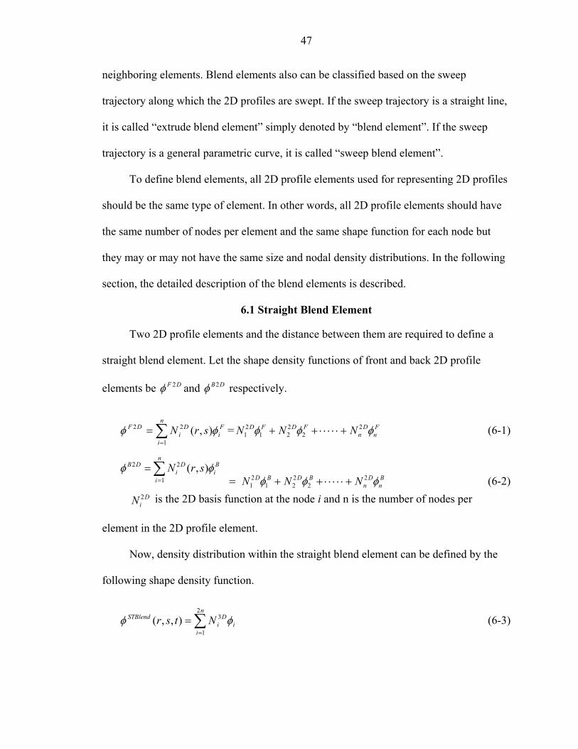
47
neighboring elements. Blend elements also can be classified based on the sweep
trajectory along which the 2D profiles are swept. If the sweep trajectory is a straight line,
it is called “extrude blend element” simply denoted by “blend element”. If the sweep
trajectory is a general parametric curve, it is called “sweep blend element”.
To define blend elements, all 2D profile elements used for representing 2D profiles
should be the same type of element. In other words, all 2D profile elements should have
the same number of nodes per element and the same shape function for each node but
they may or may not have the same size and nodal density distributions. In the following
section, the detailed description of the blend elements is described.
6.1 Straight Blend Element
Two 2D profile elements and the distance between them are required to define a
straight blend element. Let the shape density functions of front and back 2D profile
elements be and respectively. DF 2φ DB2φ
∑=
=n
i
Fi
Di
DF srN1
22 ),( φφ = (6-1) Fn
Dn
FDFD NNN φφφ 22
221
21 +⋅⋅⋅⋅⋅++
∑=
=n
i
Bi
Di
DB srN1
22 ),( φφ (6-2) = B
nD
nBDBD NNN φφφ 22
221
21 +⋅⋅⋅⋅⋅++
DiN 2 is the 2D basis function at the node i and n is the number of nodes per
element in the 2D profile element.
Now, density distribution within the straight blend element can be defined by the
following shape density function.
∑=
=n
ii
Di
STBlend Ntsr2
1
3),,( φφ (6-3)

48
The basis functions for interpolating the nodal densities are designed to give linear
interpolation in the parametric direction t that is the desired direction of depth. The
following equation shows the basis function at the node i.DiN 3
),()1(21),,( 23 srNttsrN D
iD
i += for ni .....1= at the front face of the element
),()1(21),,( 23 srNttsrN D
iD
j −= for inj += at the back face of the element (6-4)
The mapping from the parametric space to the real space for the straight blend
element can be defined as
∑=
=n
i
Di
Di tsrMtsr
2
1
33 ),,(),,( XX (6-5)
Di3X and are the nodal coordinates and the mapping basis function at the node
i respectively. As in the previous chapter, it is assumed that the mid-edge nodes are at the
mid point of the edges and that the center node is at the centroid so that the trilinear
mapping functions defined in Eq. 5-6 can be used.
DiM 3
The cross-sectional shape at the common face between elements is identical to the
2D primitive used for creating the straight blend element. Therefore the blended solid
defined by the straight blend element has the following properties.
Property 6.1-1: The blended solid represented using the straight blend elements
satisfies C0 continuity at the interface between each neighboring element.

49
Element B
Element A
Neighboring face[t= -1 at Element A, t= 1 at Element B]
t = -1 atElement B
t = 1 atElement A
bφφ =
bφφ >
bφφ =
Figure 6-1. Two neighboring straight blend elements having quadrateral 9 node elements as 2D profile
Proof: It can be verified by showing that the density distributions at t = -1 at the
element A and t = 1 at the element B are identical to the density distribution of the 2D
profile element used for the common face. Therefore the shape of interest at the common
face between two neighboring elements is same as the 2D profile used.
DBA
n
i
Bi
Di
STBlendA srNsr 2
1
2 ),()1,,( φφφ ==− ∑=
at the element A
DFB
n
i
Fi
Di
STBlendB srNsr 2
1
2 ),()1,,( φφφ == ∑=
at the element B (6-6)
DFB
DBA
22 φφ = because the same profile element is used for representing the back
face of the element A and the front face of the element B.
As mentioned earlier, the 2D profile elements may or may not have the same
density distribution. If the density distributions of the front and back 2D profile elements
are identical, the surfaces connecting the front and back 2D profiles have the following
property.

50
Property 6.1-2. The surface connecting the front and the back 2D profiles in the
straight blend element is composed of straight lines that connect points having the same r
and s but different t value (i.e. t = -1 and t =1 respectively) only if . Bi
Fi φφ =
X(r*, s*, -1)
X(r*, s*, 1)
X(r*, s*, t)Front face where t=1
Back face where t = -1
bφφ ≥bφφ ≥
Figure 6-2. A straight blend element having quadratic 9 node elements as 2D profiles
Proof: If the density distribution for the front and the back 2D profile elements are
the same, the shape density function for the straight blend element can be obtained by
applying the condition as follows. Bi
Fii φφφ ==
∑∑==
=
−++=
n
ii
Di
n
ii
Di
STBlend srNttsrN1
2
1
2 ),()1(21)1(
21),( φφφ (6-7)
Eq. 6-7 shows that the cross-sectional shapes along the parametric direction t are
invariant with respect to the t in the parametric space. Suppose (r*,s*) is the parametric
coordinates of a point on the boundary so that (boundary density) then
X(r
bD sr φφ =),( **2
*, s*, t) is the position vector of a point on the curve along the surface of the solid
connecting points on the front and back faces that share the same parametric coordinates
(r*,s*). It would now be shown that this curve is a straight line.

51
n n2D * * F 2D * * Bi i i
i 1 i 1n n
* * 2D * * F 2D * * Bi i i
i 1 i 1n n
2D * * F 2D * * Bi i i
i 1 i 1
1 1N (r ,s ) (1 t)x N (r ,s ) (1 t)x2 2x1 1X(r ,s , t) y N (r ,s ) (1 t)y N (r ,s ) (1 t)y2 2
z1 1N (r ,s ) (1 t)z N (r ,s ) (1 t)z2 2
= =
= =
= =
+ + −
= = + + −
+ + −
∑ ∑
∑ ∑
∑ ∑
i
i
i
BF tt XX )1(21)1(
21
−++= (6-8)
In the above equation, and are the nodal coordinates at
the front and the back face of the straight blend element respectively and and are
defined as
),,( Fi
Fi
Fi zyx ),,( B
iBi
Bi zyx
FX BX
=
∑
∑
∑
=
=
=
n
i
Fi
Di
n
i
Fi
Di
n
i
Fi
Di
F
zsrN
ysrN
xsrN
1
**2
1
**2
1
**2
),(
),(
),(
X and (6-9)
=
∑
∑
∑
=
=
=
n
i
Bi
Di
n
i
Bi
Di
n
i
Bi
Di
B
zsrN
ysrN
xsrN
1
**2
1
**2
1
**2
),(
),(
),(
X
Eq. 6-8 represents a line equation connecting the point and . From Eq. 6-7
the density values at and are same and the densities through the line is also same.
Therefore it is verified that the surface is composed of straight lines connecting two
points having the same r and s and different t = –1 and t = 1 respectively. Such a surface
is known as a lofted surface (or ruled surface) [Filip and Ball, 1989]. Intuitively, it is
clear that in general when the 2D profile elements defining the blend element have
different density distributions the blending surfaces are not guaranteed to be lofted
surfaces.
FX BX
FX BX
Investigating cross section shapes of the blend element along the parametric t
direction, the following property can be obtained.

52
Property 6.1-3. The cross-sectional shape of the straight blend element at a
certain parameter t* is a parallelogram if the mid-edge nodes are at the center of each
edge and mid-face node is at the centroid of the face.
t =1 t = -1t = t*
r = 1
s = 1
r = -1
s = -1
r = 1
s = 1
r = -1
s = -1
X(1,1, t*)X(-1,1, t*)
X(-1,-1, t*) X(1,-1, t*)
1
2
3
4
8
5
6
7
Figure 6-3: Cross section at a certain t* in the straight blend element
Proof: To prove that the cross-section is a parallelogram it is first shown that the
edges of the cross-section are straight lines. It can be assumed that the mapping basis
functions are tri-linear regardless of the number of nodes in the element if the mid-edge
nodes are at midpoint of the edges and mid face nodes are at the centroid of the face.
Therefore the mapping equation can be expressed as
8
ii 1
(r,s, t) M (r,s, t)=
= ∑X iX (6-10)
In the above equations Mi are the trilinear basis functions and Xi are the nodal
coordinate points in the global coordinate system. Expanding the above equation by
substituting the trilinear basis functions for Mi(r,s,t), yields,

53
87
654
321
)1)(1)(1(81)1)(1)(1(
81
)1)(1)(1(81)1)(1)(1(
81)1)(1)(1(
81
)1)(1)(1(81)1)(1)(1(
81)1)(1)(1(
81
XX
XXX
XXXX
tsrtsr
tsrtsrtsr
tsrtsrtsr
−−++−−−+
−+−+−++++−++
+−−+++−++++=
(6-11)
At any cross-section of the element t is constant so it will be denote as t*. The
equation of the boundaries of the element at this cross-section can be obtained by setting
parametric coordinates r and s to –1 or 1.
Consider the edge where r = 1, the equation of the edge, X(1,s,t*), can be expressed
as
8
541
*)1)(1(41
*)1)(1(41*)1)(1(
41*)1)(1(
41*),,1(
X
XXXX
ts
tstststs
−−+
−+++−+++= (6-12)
Rearranging,
−++−+
−+++= 8451 *)1(
21*)1(
21)1(
21*)1(
21*)1(
21)1(
21*),,1( XXXXX ttsttsts
Since t*, X1,X5,X4 and X8 are constants, it is clear that the equation of X is that of a
straight line where only s is a variable. Similarly it can be verified that other three edges
defined by r = 1, s = -1 and s = 1 are also straight lines. Now to show that the
quadrilateral defined by these four straight lines is a parallelogram it needs to be verified
that the diagonal of this quadrilateral bisect each other.
Let four vertices of the cross-section of the element at a given t* be , , and
respectively.
*1X *
2X *3X
*4X
5*
1**
1* )1(
21)1(
21),1,1( XXXX ttt −++==
6*
2**
2* )1(
21)1(
21),1,1( XXXX ttt −++==−

54
7*
3**
3* )1(
21)1(
21),1,1( XXXX ttt −++==−−
8*
4**
4* )1(
21)1(
21),1,1( XXXX ttt −++==− (6-13)
The mid point of each diagonal can be represented by
+−+++=
+ ))(1(21))(1(
21
21
2 75*
31*
*3
*1 XXXXXX tt
+−+++=
+ ))(1(21))(1(
21
21
2 86*
42*
*4
*2 XXXXXX tt (6-14)
From the fact that 2D profile elements are parallelograms, the following equations
can be obtained.
224231 XXXX +
=+ and
228675 XXXX +
=+ (6-15)
Applying the above conditions to Eq.6-14, the following relationship can be
obtained.
22
*4
*2
*3
*1 XXXX +
=+ (6-16)
Therefore the midpoints of the two diagonals are the same thus proving that the
cross-section is a parallelogram.
This is a very important property because it can be used for the mapping from the
global coordinates to the parametric coordinates. Once it is verified that the cross-section
shape of the straight blended element at a certain parametric coordinate t* is a
parallelogram, then two-dimensional mapping techniques can be used for finding the
parametric coordinates r and s.
Examples of solids created by blending 2D profiles are shown in the following
figure where four 2D profiles are used for both examples. Figure 6-4A shows the

55
blending between circular shapes and figure 6-4B shows the blending between circular
and rectangular shapes.
(A) (B)
Figure 6-4. Examples of straight blend using blend elements
6.2 Smooth Blend Element
Smooth blend elements construct a C1 continuous blended solid between 2D
profile elements defined along a straight line. The shape density function for the smooth
blend element can be defined by
∑=
+=n
iti
Dtii
Di
SMBlend NNtsr2
1
33 )(),,( φφφ (6-17)
iφ and tiφ are the nodal density and its corresponding tangent component at the
node i respectively. The basis functions for interpolating the nodal densities are designed
to give Hermite interpolation in the parametric direction t. The following shows the basis
function and at the node i. DiN 3 D
tiN 3
DiN 3 =
+
−
+ 32
2
212
213 ttN D
i = for i12 HN Di n.....1=
DitN 3 =
+
+
+
−32
2
21
21 ttN D
i = for i22 HN Di n.....1= (6-18)

56
DjN 3 =
+
+
+
−32
2
212
2131 ttN D
i = for 32 HN Di inj +=
DtjN 3 =
+
+
+
−+ 32
2
21
212
21 tttN D
i = for 42 HN Di inj +=
A composite Hermite curve is guaranteed to be C1 continuous regardless of the
tangent at the nodes. However, to set the tangent components at each node automatically,
the following two additional conditions are used. First, the second derivative at the end
each element should be equal to that at the beginning of the adjacent element. Second, the
second-order derivatives are set to zero at both ends of the primitive. According to these
conditions, the following linear equations are obtained, by which an automatic method
for setting the tangent components can be achieved. The following equation is a matrix
form for N simultaneous linear equations. Therefore, the tangent components can be
computed by solving the following equation.
210001410:0141:0......::........::......::.......0:1410:01410........0012
−'
'1
'3
'2
'1
:::::
N
N
RR
RRR
= (6-19)
−−
−−−
−
−
1
2
24
13
12
3333
:::::
333333
NN
NN
RRRR
RRRRRR
In the above equation, = φiR i and ' = φiR ti . In the smooth blend element, the
mapping from the parametric space to the real space can be performed as
)),,(),,((),,( 332
1
33 Dti
Dti
n
i
Di
Di tsrMtsrMtsr XXX += ∑
=
(6-20)

57
Di3X and are nodal coordinates and its tangent components at the node i.
and are mapping basis functions that are identical to
Dti3X
DiM 3 D
tiM 3 DiN 3
and DtiN 3
3= X
respectively for this element. is computed from Eq. 6-19 setting Dti3X D
i iR and
' = 3X DiR ti . The following property is proved to show that the solid created using the
smooth blend elements has C1 continuity along the parametric coordinate t.
Property 6.2-1. The blended solid using the smooth blend elements satisfies C1
continuity at the interface between adjacent elements.
Element B
Element A
Common face[t= -1 at Element A, t= 1 at Element B]
t = -1 atElement B
t = 1 atElement A
bφφ ≥
)1,,()1,,( srsr EBEA φφ −∇=−∇−
Figure 6-5. Two neighboring smooth blend elements having quadratic 9 node elements as 2D profile
Proof: This property can be verified by showing that the surface normal vector is
continuous at the interface between each neighboring element. Suppose the face of
interest is the back face (i.e. t = -1) in the element A denoted by EA and the front face
(i.e. t = 1) in the element B denoted by EB as shown in figure 6-5. The surface normal
vector is computed by gradient of the shape density function or normal to the element
surface in this system. The following is the formula for computing the gradient of the
shape density function with respect to the global coordinates x, y, z.

58
[ ]
∂∂∂∂∂∂
=
∂∂∂∂∂∂
=∇ −
t
s
r
z
y
x
φ
φ
φ
φ
φ
φ
φ 1J Where, the Jacobian matrix [ ]
∂∂
∂∂
∂∂
∂∂
∂∂
∂∂
∂∂
∂∂
∂∂
=
tz
ty
tx
sz
sy
sx
rz
ry
rx
J (6-21)
Let the shape density function at the element A and the element B be EAφ and EBφ
respectively, then
[ ]BEAti
BEAi
FEAti
FEAi
n
i
DiEA tHtHtHtHsrNtsr φφφφφ )()()()(),(),,( 4321
1
2 +++= ∑=
[ ]BEBti
BEBi
FEBti
FEBi
n
i
DiEB tHtHtHtHsrNtsr φφφφφ )()()()(),(),,( 4321
1
2 +++= ∑=
(6-22)
Since both element A and element B are sharing the 2D profile element at the
common face, the density distributions at the back face of the element A and the front
face of the element B are identical. Therefore,
FEBi
BEAii φφφ == and (6-23) F
EBtiBEAtiti φφφ ==
Differentiating EAφ and EBφ with respect to r, s and t and thereafter substituting –1
for the parameter t at the element A and 1 for the parameter t at the element B into Eq. 6-
22 and applying Eq. 6-21.
rsr
rsrN
rsr EB
n
ii
DiEA
∂∂
=∂
∂=
∂−∂ ∑
=
)1,,(),()1,,(1
2 φφ
φ
ssr
ssrN
ssr EB
n
ii
DiEA
∂∂
=∂
∂=
∂−∂ ∑
=
)1,,(),()1,,(1
2 φφ
φ
tsr
srNtsr EB
n
iti
Di
EA
∂∂
==∂
−∂ ∑=
)1,,(),(
21)1,,(
1
2 φφ
φ (6-24)
Similarly, the above procedure for x, y and z instead of φ can be applied.
Now, let x, y and z be and with respect to the
corresponding elements. Then
EAx EAy EAz EBx EBy EBz
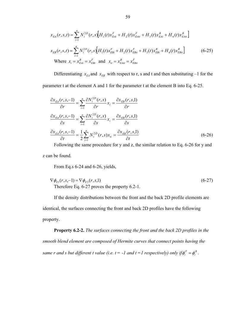
59
[ ]BEAti
BEAi
FEAti
FEAi
n
i
DiEA xtHxtHxtHxtHsrNtsrx )()()()(),(),,( 4321
1
2 +++= ∑=
[ ]BEBti
BEBi
FEBti
FEBi
n
i
DiEB xtHxtHxtHxtHsrNtsrx )()()()(),(),,( 4321
1
2 +++= ∑=
(6-25)
Where and FEBi
BEAii xxx == F
EBtiBEAtiti xxx ==
Differentiating and with respect to r, s and t and then substituting –1 for the
parameter t at the element A and 1 for the parameter t at the element B into Eq. 6-25.
EAx EBx
rsrx
xr
srNr
srx EBn
ii
DiEA
∂∂
=∂
∂=
∂−∂ ∑
=
)1,,(),()1,,(1
2
ssrx
xs
srNssrx EB
n
ii
DiEA
∂∂
=∂
∂=
∂−∂ ∑
=
)1,,(),()1,,(1
2
tsrx
xsrNtsrx EB
n
iti
Di
EA
∂∂
==∂
−∂ ∑=
)1,,(),(
21)1,,(
1
2 (6-26)
Following the same procedure for y and z, the similar relation to Eq. 6-26 for y and
z can be found.
From Eq.s 6-24 and 6-26, yields,
)1,,()1,,( 21 srsr EE φφ ∇=−∇ (6-27) Therefore Eq. 6-27 proves the property 6.2-1.
If the density distributions between the front and the back 2D profile elements are
identical, the surfaces connecting the front and back 2D profiles have the following
property.
Property 6.2-2. The surfaces connecting the front and the back 2D profiles in the
smooth blend element are composed of Hermite curves that connect points having the
same r and s but different t value (i.e. t = -1 and t =1 respectively) only if . Bi
Fi φφ =

60
X(r*, s*, -1)
X(r*, s*, 1)
X(r*, s*, t)Front face where t=1
Back face where t = -1
bφφ ≥bφφ ≥
Figure 6-6. A smooth blend element having quadratic 9 node elements as 2D profile
Proof: If the density distributions for the front and the back 2D profile elements are
same (i.e. ), it implies that all tangential componentsBi
Fi φφ = tiφ are zeros according to
Eq.6-22. Therefore the density function can be simplified as follows.
∑∑==
+
+
+
−+
+
−
+
=n
i
Bi
Di
n
i
Fi
Di
SMBlend ttsrNttsrN1
322
1
322
212
2131),(
212
213),( φφφ
Bi
Fii φφφ ==Applying the condition , then
∑=
=n
ii
Di
SMBlen srN1
2 ),( φφ (6-28)
The above equation shows that the cross-sections along the direction of t in the
parametric coordinate system are invariant. Let (r*, s*) be the parametric coordinate of a
point on the boundary of the solid so that (boundary density), then density
value at every point on a straight line connecting (r
bD sr φφ =),( **2
*, s*, -1) and (r*, s*, 1) in the
parametric coordinate system is bφ because Eq. 6-28 shows that density is invariant with
respect to t. Therefore, this line is guaranteed to be on the surface of the solid. The
parametric equation of the line mentioned above in the global coordinate system is

61
[ ]
[ ]
[ ]
+++
+++
+++
=
=
∑
∑
∑
=
=
=
Bti
Bi
Fti
Fi
n
i
Di
Bti
Bi
Fti
Fi
n
i
Di
Bti
Bi
Fti
Fi
n
i
Di
ztHztHztHztHsrN
ytHytHytHytHsrN
xtHxtHxtHxtHsrN
zyx
tsr
)()()()(),(
)()()()(),(
)()()()(),(
),,(
43211
**2
43211
**2
43211
**2
**X
= (6-29) Bt
BFt
F tHtHtHtH XXXX )()()()( 4321 +++This is a Hermite curve equation where
=
=
∑
∑
∑
=
=
=
n
i
Fi
Di
n
i
Fi
Di
n
i
Fi
Di
F
F
F
F
zsrN
ysrN
xsrN
zyx
1
**2
1
**2
1
**2
),(
),(
),(
X and (6-30)
=
=
∑
∑
∑
=
=
=
n
i
Fti
Di
n
i
Fti
Di
n
i
Fti
Di
Bt
Bt
Bt
Ft
zsrN
ysrN
xsrN
zyx
1
**2
1
**2
1
**2
),(
),(
),(
X
=
=
∑
∑
∑
=
=
=
n
i
Bi
Di
n
i
Bi
Di
n
i
Bi
Di
B
B
B
B
zsrN
ysrN
xsrN
zyx
1
**2
1
**2
1
**2
),(
),(
),(
X and (6-31)
=
=
∑
∑
∑
=
=
=
n
i
Bti
Di
n
i
Bti
Di
n
i
Bti
Di
Bt
Bt
Bt
Bt
zsrN
ysrN
xsrN
zyx
1
**2
1
**2
1
**2
),(
),(
),(
X
This curve is also a cardinal spline if it satisfies the following equation.
( )FEA
BEB
BEBtt
FEAt XXXXX −=++ 34 (6-32) Where F
EBtBEAtt XXX ==
This equation can be written as follows.
−
−
−
=
++
++
++
∑
∑
∑
∑
∑
∑
=
=
=
=
=
=
n
i
FEAi
BEBi
Di
n
i
FEAi
BEBi
Di
n
i
FEAi
BEBi
Di
n
i
BEBtiti
FEAti
Di
n
i
BEBtiti
FEAti
Di
n
i
BEBtiti
FEAti
Di
zzsrN
yysrN
xxsrN
zzzsrN
yyysrN
xxxsrN
1
**2
1
**2
1
**2
1
**2
1
**2
1
**2
),(
),(
),(
3
4),(
4),(
4),(
Or
(∑∑==
−=++n
i
FEAi
BEBi
Di
n
i
BEBtiti
FEAti
Di srNsrN
1
**2
1
**2 ),(34),( XXXXX ) (6-33)

62
Since the solid element is defined such that ( )FEAi
BEBi
BEBtiti
FEAti XXXXX −=++ 34
(see Eq. 6-19), the above equation is automatically correct. Therefore when density
distribution is identical for front and back faces the smooth blend primitives have C2
continuity along the t direction at the common face between neighboring solid elements
because curves on its surface in the parametric direction t are Cardinal splines.
However, in general when 2D profile elements defining the smooth blend element
have different density distributions, the resulting blended solid’s boundary is not
composed of cardinal splines.
Investigating cross-sectional shapes of the smooth blend element along the
parametric direction t, the following property can be obtained.
Property 6.2-3. The cross-section shape of the smooth blend element at a certain
parameter t* is a parallelogram if the mid-edge nodes are at the center of each edge and
mid-face node is at the centroid of the face.
E2
E1
Common face[t= -1 at element A , t= 1 at element B]
t = -1 at element B
t = 1 atelement A
t = t*
r = 1
s = 1
r = -1
s = -1
X(1,1, t*)X(-1,1, t*)
X(-1,-1, t*) X(1,-1, t*)
1
1
4
3
2
5
8
7
6
10
1112
9
Figure 6-7. Cross section at a certain t* in smooth blend elements

63
Proof: To prove this property, it is first verified that it is true in the smooth blend
element. Initially it is assumed that 4 node quadrilateral elements are used for the 2D
profile elements. The mapping equation as shown in figure 6-7 is
∑=
+=8
1
)),,(),,((),,(i
titiii tsrNtsrNtsr XXX (6-34)
Consider the edge where r = 1, for any cross-section t=t*. The points on this edge,
X, can be written as
8454
4212
8353
4111
)()1(21)()1(
21
)()1(21)()1(
21
)()1(21)()1(
21
)()1(21)()1(
21),,1(
tt
tt
tHstHs
tHstHs
tHstHs
tHstHsts
XX
XX
XX
XXX
−+++
−+++
−+++
−++=
(6-35)
From Eq. 6-19, it is known that,
1551 332 XXXX −=+ tt
4884 332 XXXX −=+ tt
19951 334 XXXXX −=++ ttt
4121284 334 XXXXX −=++ ttt According to the above relationships, X(1,s,t) can be simplified as
84834241
54531211
)()()()()1(21
)()()()()1(21),,1(
tt
tt
tHtHtHtHs
tHtHtHtHsts
XXXX
XXXXX
+++−+
++++= (6-36)
Since t, X1, X5, X4, X8, Xt1, Xt5, Xt4 and Xt8 are constants, therefore the final form
of X(1,s,t) is a line equation where the variable is s. Similarly it can be verified that other
three edges defined by r = 1, s = -1 and s = 1 are also straight lines. This proves that the

64
cross sectional shape of the blend element at a certain t* is a quadrilateral. This
quadrilateral is a parallelogram if its diagonals bisect each other as shown below.
Let four vertices of the cross-sectional shape be , , and respectively. *1X *
2X *3X *
4X
54531211*1
* )()()()(),1,1( tt tHtHtHtHt XXXXXX +++==
64632221*2
* )()()()(),1,1( tt tHtHtHtHt XXXXXX +++==−
74733231*3
* )()()()(),1,1( tt tHtHtHtHt XXXXXX +++==−−
84834241*4
* )()()()(),1,1( tt tHtHtHtHt XXXXXX +++==− (6-37) The midpoints of the two diagonals are
[]))(())((
))(())((21
2754753
312311
*3
*1
tt
tt
tHtH
tHtH
XXXX
XXXXXX
++++
+++=+
[]))(())((
))(())((21
2864863
422421
*4
*2
tt
tt
tHtH
tHtH
XXXX
XXXXXX
++++
+++=+
(6-38)
Again from Eq. 6-19, the followings can be obtained.
1551 332 XXXX −=+ tt
2662 332 XXXX −=+ tt
3773 332 XXXX −=+ tt
4884 332 XXXX −=+ tt
The above equations can be combined to yield the following equations.
)(3)(3)()(2 31757531 XXXXXXXX +−+=+++ tttt
)(3)(3)()(2 42868642 XXXXXXXX +−+=+++ tttt (6-39) From the fact that the 2D profile elements used to define the smooth blend are
parallelograms,
224231 XXXX +
=+ and
228675 XXXX +
=+ (6-40)
Therefore, the following equation can be obtained from Eq. 6-39.
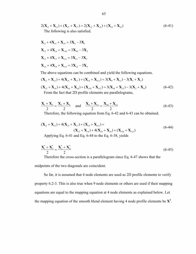
65
)()(2)()(2 86427531 tttttttt XXXXXXXX +++=+++ (6-41) The following is also satisfied.
19951 334 XXXXX −=++ ttt
2101062 334 XXXXX −=++ ttt
3111173 334 XXXXX −=++ ttt
4121284 334 XXXXX −=++ ttt
The above equations can be combined and yield the following equations.
)(3)(3)()(4)( 311191197531 XXXXXXXXXX +−+=+++++ tttttt
)(3)(3)()(4)( 42121012108642 XXXXXXXXXX +−+=+++++ tttttt (6-42) From the fact that 2D profile elements are parallelograms,
224231 XXXX +
=+ and
221210119 XXXX +
=+ (6-43)
Therefore, the following equation from Eq. 6-42 and 6-43 can be obtained.
)()(4)()()(4)(
12108642
1197531
tttttt
tttttt
XXXXXXXXXXXX
+++++=+++++
(6-44)
Applying Eq. 6-41 and Eq. 6-44 to the Eq. 6-38, yields
22
*4
*2
*3
*1 XXXX +
=+ (6-45)
Therefore the cross-section is a parallelogram since Eq. 6-47 shows that the
midpoints of the two diagonals are coincident.
So far, it is assumed that 4 node elements are used as 2D profile elements to verify
property 6.2-3. This is also true when 9 node elements or others are used if their mapping
equations are equal to the mapping equation at 4 node elements as explained below. Let
the mapping equation of the smooth blend element having 4 node profile elements be X4.

66
∑
∑
=++
=
++
+=
4
1)4(442
4
131
4
)),(),((
)),(),((),,(
iitiii
itiiii
srNHsrNH
srNHsrNHtsr
XX
XXX (6-46)
The following shows the mapping function at the smooth blend element where
quadratic elements having n nodes are used for 2D profile elements.
∑
∑
=++
=
++
+=
n
initinii
n
itiiii
n
srNHsrNH
srNHsrNHtsr
1)(42
131
)),(),((
)),(),((),,(
XX
XXX (6-47)
If the mapping equation in the 2D profile element having n nodes is same as the
mapping equation in the 4 node quadrilateral element, i.e., if
(as proved in Chapter 4 for 9 node elements, Eq. 4-8), the
following is also true.
4
1 1( , ) ( , )
n
i i ii i
N r s N r s= =
=∑ ∑X iX
),,(),,(4 tsrtsr nXX = (6-48) This property can be used for the mapping from the global coordinates to the
parametric coordinates. Once it is verified that the cross-section shape of the smooth
blend element at a certain parametric coordinate t* is a parallelogram, then two-
dimensional mapping techniques can be used for finding the parametric coordinates r and
s.
Examples of solids created by blending 2D profiles are shown in the following
figure where four 2D profiles are used for both examples. Figure 6-8A shows the
blending between circular shapes and figure 6-8B shows the blending between circular
and rectangular shapes.

67
(A) (B)
Figure 6-8. Examples of Smooth blend using blend elements
6.3 Sweep Blend
The sweep blend element is used to represent a solid obtained by sweeping 2D
profiles represented by 2D implicit solid elements along an arbitrary parametric curve.
Therefore, the sweep blend element is defined by specifying the 2D profile elements, a
sweep trajectory as well as an orientation vector that controls the orientation
of the swept profile. The detailed description regarding sweep trajectories is explained in
Chapter 5.
( )tR )(td
Two different types of blending functions, straight and smooth blending can be
applied to sweep blend too. Therefore all properties illustrated already in the previous
sections are also applicable to sweep blend.
Since the nodal coordinates of the sweep blend elements are represented with
respect to the local coordinate system as L(r,s,t) =u(r,s,t) v(r,s,t) tT, the mapping
between the parametric coordinates and the local coordinates u and v can be expressed as
∑=
=n
iii tsrNutsru
1),,(),,(

68
∑=
=n
iii tsrNvtsrv
1),,(),,( (6-49)
where, ui, vi are nodal coordinates of the sweep solid element with respect to the
local coordinate system. Ni(r,s,t) are basis functions for both the mapping from the
parametric coordinates r, s and t and interpolating nodal densities. Therefore the basis
functions are different with respect to the blend types such as straight blend and smooth
blend.
Examples of solids created using sweep blend element are shown in the following
figure where four 2D profiles are used for both examples. Figure 6-9A shows the sweep
straight blending between rectangular shapes and figure 6-9B shows the sweep smooth
blending between circular shapes.
(A) (B)
Figure 6-9. Examples of Sweep Blending A) Sweep straight blend B) Sweep
smooth blend

CHAPTER 7 CSG REPRESENTATION USING IMPLICIT ELEMENTS
CSG representation scheme is used for representing a solid in this solid modeling
system where implicit solid elements are used for representing primitives instead of half
spaces. The final solid is constructed by combining simple primitives using regularized
Boolean operations to define a solid as a closed region in space. It is necessary to
compute points and surface normal vectors on the boundary of the solid for graphically
displaying it. The following sections, describe the CSG tree structure used in this system,
how to compute surface normal vectors, and how to perform set-membership
classification.
7.1 Surface Normal Vectors
To graphically display primitives defined using implicit solid elements, it is
necessary to evaluate points on the surface and to compute surface normal vectors at
these points. The method for evaluating points on the surface is explained in chapter 9.
Here, the method for computing the surface normal vector at a given point on a primitive
represented by an implicit solid element is described.
To compute the surface normal vector at a given point on the boundary of a solid
represented using an implicit solid element, the point has to be first classified as inside
the element ( ) or on the boundary of the element
( r ). If the point is inside the implicit solid element, the gradient of
the density function is computed since it is a vector normal to the surface at the point of
b , 1 r 1, 1 s 1, 1 t 1φ = φ − < < − < < − < <
1 or t= 1± ±1 or s== ±
69

70
interest. The gradient of φ with respect to the global coordinates (x, y, z) can be computed
as:
[ ]
∂∂∂∂∂∂
=
∂∂∂∂∂∂
=∇ −
t
s
r
z
y
x
φ
φ
φ
φ
φ
φ
φ 1J (7-1)
Where [ ]
∂∂
∂∂
∂∂
∂∂
∂∂
∂∂
∂∂
∂∂
∂∂
=
tz
ty
tx
sz
sy
sx
rz
ry
rx
J (7-2)
The [J] matrix or the Jacobian matrix can be easily obtained since the mapping
expresses x, y and z as functions of r, s and t. For instance, the first component of the
Jacobian matrix can be expressed as where ∑=
=n
tii tsrNxx
1),,( .
( ) ( ) ( )r
tsrNxr
tsrNxr
tsrNxr
tsrNx
rx nn
n
iii
∂∂
++∂
∂+
∂∂
=∂
∂
=∂∂ ∑
= ),,(),,(),,(),,(
22111 (7-3)
Similarly, the other components of the first column are
( ) ( ) ( )s
tsrNxs
tsrNxs
tsrNxs
tsrNx
sx nn
n
iii
∂∂
++∂
∂+
∂∂
=∂
∂
=∂∂ ∑
= ),,(),,(),,(),,(
22111
( ) ( ) ( )t
tsrNxt
tsrNxt
tsrNxt
tsrNx
tx nn
n
iii
∂∂
++∂
∂+
∂∂
=∂
∂
=∂∂ ∑
= ),,(),,(),,(),,(
22111 (7-4)
The second and third columns of the Jacobian matrix can be computed by replacing
x with y and z in Eq. (7-3) to (7-4) respectively.

71
Note that the gradient points towards the direction of increasing density φ that is
towards the inside of the solid. Therefore, the surface normal is set in the opposite
direction as . = −∇φn
The actual equations for finding each component of the Jacobian matrix depend
upon the mapping functions of r, s and t. Therefore, the solid elements having different
mapping functions need to be treated accordingly. Since extrude, revolve and sweep
elements have their own mapping functions that are different from each other, they have
their own corresponding equations for finding the components of the Jacobian matrix as
follows.
In extrude elements including extrude blend elements, Eq. 7-3 and Eq. 7-4 can be
used directly because the global coordinates (x, y, z) are just functions of the parametric
coordinates (r, s, t). Therefore each component of the Jacobian matrix can be computed
by just differentiating the mapping function with respect to the parametric coordinates (r,
s, t). However revolve elements use the cylindrical coordinate system whereas the
extrude elements use the Cartesian coordinates system. Therefore one more step is
required to find the surface normal vectors for revolve elements. The following is an
example where the first components of the Jacobian matrix is computed.
rZ
Zx
rx
rR
Rx
rx
∂∂
∂∂
+∂θ∂
θ∂∂
+∂∂
∂∂
=∂∂ (7-5)
Here Rx
∂∂ ,
θ∂∂x and
Zx
∂∂ can be derived from Eq. 5-9 explicitly.
θθ sincos xx caRx
−=∂∂ , θθ
θcossin RcRax
xx −−=∂∂ and xb
Zx
=∂∂ (7-6)
Since R, θ and Z are represented by the interpolation using the nodal basis
functions, their differentiations are

72
r
tsrNR
rR
n
iii
∂
∂
=∂∂ ∑
=
),,(1
r
tsrN
r
n
iii
∂
∂
=∂∂ ∑
=
),,(1θ
θ (7-7)
r
tsrNZ
rZ
n
iii
∂
∂
=∂∂ ∑
=
),,(1
In sweep elements, the following equations are used for computing the each
component of the Jacobian matrix where the notations used in Eq. 7-8 are followed from
chapter 5.
∑∑==
+=
=n
ii
Di
n
ii
Di v
drsrdNu
drsrdN
drdzdrdydrdx
drtsrd
1
2
1
2 ),(),(),,( mnP
∑∑==
+=
=n
ii
Di
n
ii
Di v
dssrdNu
dssrdN
dsdzdsdydsdx
dstsrd
1
2
1
2 ),(),(),,( mnP (7-8)
dtd
dtdzdtdydtdx
dttsrd R(t)P
=
=),,(
If the point of interest is on the boundary of the element, the surface normal vector
is equal to the vector normal to the element face on which the point is located. The
position vector of an arbitrary point within the element is expressed as follows ),,( tsrR

73
n
i ii 1n
i ii 1n
i ii 1
x M (r,s, t)x
(r,s, t) y y M (r,s, t)z
z M (r,s, t)
=
=
=
= =
∑
∑
∑
R (7-9)
The six faces of a hexahedral element are represented as , ,
, , ,
),,1( tsR ),,1( ts−R
),1,( trR ),1,( tr −R )1,,( srR )1,,( −srR
,,1( tsR
respectively. Since these are parametric
equations of surfaces, the normal vector for any point on these faces can be easy
computed as the cross product of the tangent vectors along the parametric directions. For
example, normal vector to the face is )
(1,s, t) (1,s, t)s t
∂ ∂= ×
∂ ∂R Rn (7-10)
Similarly, the normal vectors can be computed on the other five faces. Table 7-1
shows the normal vectors on all six faces of the element.
Table 7-1 Surface normal vectors on the boundary of the element Element Face Normal Vector Element Face Normal Vector
),,1( tsR t
tss
ts∂
∂×
∂∂ ),,1(),,1( RR
),,1( ts−R s
tst
ts∂−∂
×∂−∂ ),,1(),,1( RR
),1,( trR r
trt
tr∂
∂×
∂∂ ),1,(),1,( RR
),1,( tr −R t
trr
tr∂
−∂×
∂−∂ ),1,(),1,( RR
)1,,( srR s
srr
sr∂
∂×
∂∂ )1,,()1,,( RR
)1,,( −srR rsr
ssr
∂−∂
×∂
−∂ )1,,()1,,( RR
Surface normal is ambiguous for points along the edges and vertices of the implicit
solid element unless a face of the element is also specified whose normal is to be
computed at the point.

74
7.2 Set membership classification within an element
An important requirement for any unambiguous solid model representation is that
one should be able to classify a given point as being inside, on, or outside the solid.
Algorithms for such point set member classification are non-trivial for B-Reps. For
traditional implicit surfaces, one can use the value of the implicit surface function to
determine which side of the surface a point lies on. However, for primitives defined using
implicit solid elements, the density function is expressed as a function of the parametric
coordinates and therefore it is necessary to first map a point from the real space into the
parametric space to evaluate the density. The mapping between those two spaces is
typically non-linear. If the given point is pX then the following equations for the
parameters pr , ps and pt that corresponds to this point need to be solved.
p i i p p pM (r ,s , t )=X X (7-11) If the mapping basis functions, , are nonlinear three simultaneous non-
linear equations need to be solved. Since it is not always possible to obtain analytical
solution for such equations it is necessary to use numerical methods such as Newton-
Raphson method to find a solution. Clearly, these equations will be easier to solve if
simple basis functions for the mapping are used. For example, when a 9-node element is
used, the interpolation basis function is bicubic, but one could use a simpler bilinear (4-
node) basis functions for the mapping if the element edges are not distorted into curves
and mid-nodes are mid points of each edge. Moreover the mapping function can be
solved analytically to find the parametric coordinates from the given global coordinates
as shown in Chapter 4.
i p p pM (r ,s , t )

75
An analogous set of mapping equations for (x, y, z) can be derived for the 8-node
hexahedral element where trilinear basis functions are used. Even though for the general
case these equations are nonlinear, they reduce to linear simultaneous equations for
elements whose opposing faces are parallel. Therefore, if the shape of the element in the
real space is a parallelogram in 2D or a parallelepiped in 3D then the mapping is linear
and easy to perform in either direction.
However, in general, three nonlinear simultaneous equations need to be solved
numerically to compute the parametric coordinate. To avoid such numerical computation
3D problems are reduced to 2D problems that can be solved analytically. This is based on
the idea that the cross-sections of the implicit solid element along the sweep direction are
parallelograms and the mapping from the real space to the parametric coordinates of this
parallelogram is bilinear. All predefined 2D primitives are parallelograms so that the
mapping equations can be solved analytically.
Therefore the first step in mapping is to find the parametric value t for the given
point. When the sweep trajectory is a straight line, the parameter t* can be easily
computed by comparing the distance from the given point and the element front face and
the depth of the element. Similarly, when the sweep trajectory is an arc, the parameter t*
can be computed by comparing the angle between the given point and the element front
face and the total angle of revolution of the element.
In the case of sweep elements including sweep blend elements where the sweep
trajectories are arbitrary parametric curve equations, the nonlinearity in the mapping is
introduced by the sweep trajectory. The parameter t* can be computed as the optimal
solutions obtained by minimizing ( )t − pR X that is by finding the closest point on the
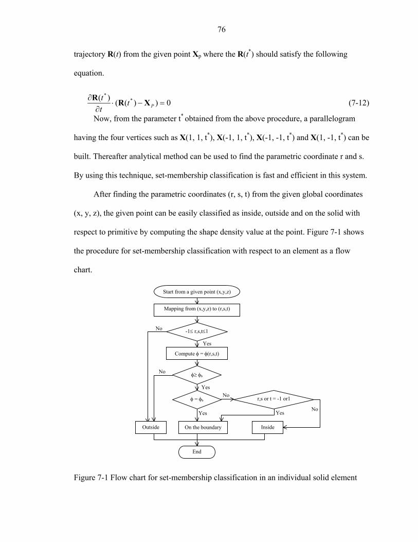
76
trajectory R(t) from the given point Xp where the R(t*) should satisfy the following
equation.
0))(()( **
=−⋅∂
∂Pt
tt XRR (7-12)
Now, from the parameter t* obtained from the above procedure, a parallelogram
having the four vertices such as X(1, 1, t*), X(-1, 1, t*), X(-1, -1, t*) and X(1, -1, t*) can be
built. Thereafter analytical method can be used to find the parametric coordinate r and s.
By using this technique, set-membership classification is fast and efficient in this system.
After finding the parametric coordinates (r, s, t) from the given global coordinates
(x, y, z), the given point can be easily classified as inside, outside and on the solid with
respect to primitive by computing the shape density value at the point. Figure 7-1 shows
the procedure for set-membership classification with respect to an element as a flow
chart.
Yes Yes
Yes
No
No
No
Outside
No
Yes
End
Inside On the boundary
r,s or t = -1 or1φ = φb
Compute φ = φ(r,s,t)
φ≥ φb
-1≤ r,s,t≤1
Mapping from (x,y,z) to (r,s,t)
Start from a given point (x,y,z)
Figure 7-1 Flow chart for set-membership classification in an individual solid element

77
7.3 Constructive Solid Geometry using Implicit Solid Elements
As mentioned earlier, CSG representation is a well-established technique for
representing solid models and is used to construct solid models by Boolean combination
of primitives that are represented either as B-Rep or using implicit half spaces. The same
approach can be used with primitives represented by the implicit solid elements. An
advantage of using the implicit surfaces is that set membership classification is
computationally less expensive than with B-Rep. Furthermore, there is no need for
expensive boundary evaluation algorithm, which is needed in the hybrid approach to
automatically construct the B-Rep model of the solid represented by the CSG tree. This
step is necessary in the hybrid approach because the B-Rep model of the Boolean result is
needed for creating the graphical display and also for subsequent operations such as set
membership classification. However, if the primitives used in the CSG tree are
represented using implicit solid elements, it is possible to directly compute the solid’s
properties, generate graphical display and perform set membership classification based
on the procedural description of the solid embodied in a CSG tree. The following figure
shows the CSG tree data structure used in this system.
(a) 2D CSG tree (b) 3D CSG tree
Primitive Node
Boolean Node
Figure 7-2 CSG tree data structure

78
The CSG tree shown in Figure 7-2 illustrates how a solid is represented in this
system. Every leaf node represents a primitive defined by implicit solid elements and the
branch node represents a Regularized Boolean type such as union, intersection and
subtraction ( respectively). Before performing Boolean operations the two
participating solids need to be positioned correctly with respect to each other. This could
be achieved by translations and rotations specified by the user but for dimension driven
editing the required transformation must be computed based on specified positioning
constraints. In this implementation, a sequential constraint imposition method [Kumar,
2000] was used to compute the transformation matrix required to impose position
constraints between solids. Typically, position constraints are specified between vertices,
edges and faces of a solid if the solid is represented using a B-Rep model. Even though
such entities are not available in implicit solid models, the nodes, edges and faces of the
implicit element itself serve as useful datum that can be used for specifying constraints.
−//∩∪
Figure 7-3 is a simple example where the 2D profile is obtained by the union of a
rectangle and a circle followed by the subtraction of an ellipse. Figure 7-4 shows a 3D
example.
U
Figure 7-3 2D Boolean operation in CSG

79
Figure 7-4 3D Constructive Solid Geometry Tree
For a primitive solid defined using a single element, the shape density value at a
point can be computed as used to classify the point as inside the solid, on the boundary of
the solid or outside the solid. When many primitives have been combined using Boolean
operations, a procedure for classifying points with respect to the Boolean results are
required. In order to apply the same procedure for the Boolean result the shape density at
every point within the solid including regions where multiple primitives may intersect
needs to be defined. This can be accomplished by using the following definition that is
commonly used in the literature on level set methods.
),max( BABA φφφ =∪ Union
),min( BABA φφφ =∩ Intersection (7-13)

80
),min( BABA φφφ −=− Subtraction In the above definitions, A B∪φ is the density at any given point within the solid
defined as the union between two solids A and B whose shape density values are Aφ and
Bφ respectively. It can be easily verified that A B∪φ will be greater than the level set value
at every point within the solid defined by the union. It is equal to the level set value at the
boundary and less than equal to outside the solid. Similar definitions are given above for
the intersection and difference between solids.
Another way to define density at every point within a solid is by using R-functions
[Shapiro, 1998], [Shapiro, Tsukanov, 1999] which can be used to define the density for
the solid defined using Boolean operations. The sign of such a function depends only on
the sign of its arguments and not their magnitude. This property can be used to define
density values at points where two or more primitives intersect. However, to use R-
functions it is necessary that every point on the boundary of the solid have value equal to
the level set value φb. In implicit solid elements, the solids boundary can be the same as
element boundary where the density need not be the level set value. Therefore, to use R-
function method the definition of the implicit solid element will have to be modified
accordingly. In this implementation, R-functions to define density for Boolean solids
were not used.
As mentioned Chapter 2, when the given point is on both the base and the
dependent solids, it is difficult to determine its set membership with respect to the
regularized Boolean result by simply comparing its set membership with respect to base
and dependent solids. In order to apply the rules of regularized Boolean operations, it is
necessary to study the neighborhood of the given point to check whether it is on the

81
boundary or the interior of the solid. Alternately, one can compare the direction of
surface normal of the solids between which the regularized set operation is being applied
[Mantyla, 1988]. This approach can be applied recursively to perform set membership
classification for arbitrarily large CSG trees. By applying this procedure the density
functions only at the primitive level are used.
As mentioned in Chapter 2, the neighborhood model enables us to classify points
with respect to the regularized Boolean when multiple normal vectors are involved. From
a theoretical point of view, the neighborhood model at a given point is easy to understand
but it is very difficult to construct an algorithm based on this model since there are
infinite points in a neighborhood that needs to be checked. In this system, a graphical
method for constructing the neighborhood model is proposed and implemented. This
method is based on the assumption that the maximum number of normal vectors involved
at a given point is three in the level of solid elements and it is convex not concave.
Therefore triangles from the normal vectors that represent half spaces can be constructed.
The detailed description for constructing triangles from the surface normal vectors is
explained in the following.
In a solid element, triangles can be constructed from the surface normal vectors as
shown where a face of the solid has one normal vector, an edge of the solid has two
normal vectors and a vertex of the solid has three normal vectors respectively.

82
nC2nC1
nB3
nB2
nB1
nA1
nA1
nB1
nB3
nB2
nC1
nC2
Figure 7-5. surface normal vectors and corresponding triangles
When there is only one surface normal vector at a given point, a triangle normal to
this vector can be constructed by the following procedure.
nA
B
C
a
bc
P
Figure 7-6: Constructing a triangle from one normal vector
In the Figure 7-6, n is the unit surface normal vector ( 1=n ). a, b and c are unit
vectors perpendicular to the surface normal vector n. a can be chosen from any arbitrary
vector perpendicular to the surface normal n. Therefore, a should satisfy the following
condition.
0=⋅ na and 1=a Then point A can be computed as
aPA s+= (7-14)

83
The scalar s is the distance from the given point P to the point A. Therefore it
defines the size of the triangle. Since the size of the triangle does not matter while
constructing neighborhood model, any value can be used for s. In this implementation 0.5
is used for s. After computing a, the vectors b can be computed by rotating a 120 degree
about axis n and similarly c can be computed by rotating b 120 degrees. Then points B
and C can be computed as.
bPB s+=
cPC s+= (7-15) When the number of surface normal vectors is two, the corresponding two triangles
can be obtained by the following procedure. Let n1 and n2 be the two unit surface normal
vectors at the point of interest.
1=1n and 1=2n
a
bEdge
n1
n2
c
d
AC
B
D
P
Figure 7-7. Constructing two triangles from two normal vectors
a is computed as the cross product of n1 and n2.
21 nna ×= (7-16) b = -a
c and d can be computed by cross product.

84
anc 1 ×=
bnd 2 ×= To use c and d vectors for constructing triangles, their direction should be verified.
Since it is assumed that each solid primitive is the intersection of half spaces that are
normal to n1 and n2 respectively, the following equations show its validity.
If , c = c. if not c = -c. 0≤⋅ cn2
If , d = d. if not d = -d. 0≤⋅ dn1
After finding vectors a, b, c and d, the points composing vertices of the triangles
can be computed as
aPA s+= , , CbPB s+= cP s+= and dPD s+= (7-17) Finally, when the number of surface normal vectors is three, the corresponding
three triangles can be obtained by the following procedure. In Figure 7-8, n1, n2 and n3
are unit normal vectors at the point of interest.
1=1n , 1=2n and 1=3n
Edgen1
n3
n2
AB
P
C
ab
c
Edge
Edge
Vertex
Figure 7-8. Constructing three triangles from three normal vectors
a is computed as the cross product between n1 and n3.
a (7-18) 31 nn ×=
If , a = a. if not a = -a. 0≤⋅ an2
Similarly,

85
b 12 nn ×=
If , b = b. if not b = -b. 0≤⋅bn3
c 23 nn ×=
If , c = c. if not c = -c. 0≤⋅ cn1
After finding vectors a, b, c and d, the points composing the vertices of the
triangles can be computed as
aPA s+= , and CbPB s+= cP s+= (7-19) After constructing the triangles for all the primitives whose boundaries pass
through the point of interest, the neighborhood at the point is constructed by performing
the Boolean operations between the triangles treating each triangle as a half space, which
divides the space into two regions inside and outside. At first, intersections between
triangles from the base and dependent solids are computed for each Boolean operation,
and then the triangles will be subdivided at the intersections. Thereafter set membership
classification of the triangles with respect to the half spaces (instead of the actual solid) is
performed to collect the valid triangles.
To classify the triangles, first the centroid Q of the triangle is computed and then
this point is classified with respect to Boolean result recursively starting from the bottom
of the CSG tree. It is assumed that the classification of the centroid is identical to the
classification of the triangle. In addition, subdivided triangles that do not contain the
point of interest are removed from the valid triangles because the neighborhood model
can be constructed without those triangles. If there are triangles at the final node, it means
that the set membership is on the solid. If there are no triangles, then it implies that the set
membership is in or out.
The above algorithm can be used for 2D or 3D CSG tree with the difference that
lines are used to represent half spaces in 2D. Figure 7-9 shows an example that shows

86
how to construct the neighborhood at a given point. As shown in Figure 7-9, the point of
interest from A and B has multiple normal vectors. Two triangles and three triangles are
derived from the solid A and B respectively. A union operation between those triangles is
performed to get the valid triangles at the union node where four triangles are obtained
after union. Therefore the point of interest can be classified as on the solid after union.
AB A B
U
Figure 7-9. Neighborhood model using graphical method
Figure 7-10 shows examples of solids created by Boolean operations using this
software implementation

87
Figure 7-10. Examples of 3D Boolean solids.

CHAPTER 8 VOLUME OF THE SOLID MODEL
8.1 Linear Approximate Step Function
Even though implicit surface equations can be used for representing the interior,
exterior and boundary of the surface, it can not be directly used to compute the volume of
the solid by integrating the equations because its values are not guaranteed to be 1 at the
interior of the solid. Therefore an approximation using a linear step function is proposed
here to construct a implicit function whose value is 1 in the interior of the solid. The
linear approximate step function used is defined as follows.
−≤
≤≤−+
≥
=
ε
εεε
ε
x
xxx
xh
022
11
)( (8-1)
Figure 8-1 Linear approximate step function graph
x
1
0.5
h(x)
ε− ε
Suppose f(x) is an implicit surface function where the region f(x) ≥ 0 is the solid,
then the zero level set is the boundary of the solid. The zero level set function can be
converted to the linear approximate step function by replacing x in Eq. 8-1 by the implicit
88

89
function f(x) that is a scalar function. Then the set-membership classification at a given
point can be performed by the linear approximate step function value as follows.
))(( xfh > 0.5 inside the solid
))(( xfh = 0.5 boundary of the solid (8-2)
))(( xfh < 0.5 outside the solid
The function provides an alternative implicit representation of the
solid such that its value changes from 0 to 1 across the boundary of the solid. It will be
therefore referred to as the function as the step function of the solid which can
be used to define the solid as per Eq. 8-2. In Eq. 8-1,
( ( )) 0.5−xh f
))(( xfh
ε is a tunable parameter. As
0→ε , the step function value becomes 1 almost everywhere in the interior of the solid.
By using this property, the volume of the solid can be directly computed by integrating
the step function of the solid.
21))(( =xfh0)( =xf
0)( >xf
0)( <xf
1))((21
≤< xfh
21))((0 <≤ xfh
Figure 8-2. Transform from the implicit surface function to its linear approximate step function
Boolean operation between two approximate step functions of the implicit
functions fA and fB can be performed by the following equations by which a new step
function representing the Boolean result can be constructed systematically.

90
)()( ABBBAABA hhhhhhhhh −+−=∪ Union operation
)()( BABABABA hhhhhhhhh −+−=∩ Intersection operation (8-3)
)()( BABBAABA hhhhhhhhh −−−=− Subtraction operation
Where and h)( AA fhh = )( BB fh=
These functions represent the step function of the Boolean between the solids
represented by fA and fB. The solid represented by this equation is not a regularized
Boolean result but is suitable for computing the volume of the solid. The difference
between ordinary Boolean result and the Regularized Boolean are lines in 2D or faces in
3d that do not contribute to the volume therefore the volume computed for ordinary
Boolean is the same as the volume of the Regularized Boolean.
Table 8-1. Simple examples for Boolean operation between approximate step functions where f1 and f2 both represent squares.
BAh ∪
BAh ∩
BAh −
1=∪BAh
21
=∪BAh 1=∪BAh1=∪BAh 1=∪BAh
1=∪BAh
21
=∪BAh
0=∩BAh
21
=∩BAh 0=∩BAh1=∩BAh 0=∩BAh
0=∩BAh
21
=∩BAh
1=−BAh
21
=−BAh 0=−BAh0=−BAh 0=−BAh
1=−BAh
21
=−BAh

91
8.2 Constructing the Step Function for the CSG Solid
A solid primitive is defined by intersections of the half spaces corresponding to the
edges of the element and region where the density function has value greater than the
level set value. The edges of the element can be defined by implicit functions defined in
the parametric space. For example, in Figure 8-3, r =1 represents the right side of the
element which divides the space into r>1 and r<1. The side where r =1 can be represented
by the implicit function f1=1-r. Similarly all boundaries of the element can be represented
by implicit functions. In Figure 8-3, all implicit functions within an element are
displayed.
1 r
s
f 1
1f 2
f 3
f 4
f 5
r
s
f 1
f 2
f 3
f 6
t
f 4f 5
f 7
(A) (B)
Figure 8-3. Implicit surfaces defining a solid within an element in the parametric space A) 2D solid element B) 3D solid element
In Figure 8-3A, the five implicit surface functions in a 2D solid element are
f1 = 1-r, f2 = 1-s, f3 = 1+r, f4 = 1+s, f5 = fφ = φ(r,s) - φb
In Figure 8-3B, the seven implicit surface functions in a 3D solid element are
f1 = 1-r, f2 = 1-s, f3 = 1+r, f4 = 1+s, f5 = 1-t, f6 = 1+t, f7 = fφ = φ(r,s,t) - φb

92
Since the Boolean operations between implicit functions in an element are all
intersections, it can be simply treated as follows because it does not depend on the order
of the Boolean operation.
In a 2D element 5432154321 ffffffefffffE hhhhhhhhh === ∩∩∩∩ φ
In a 3D element 76543217654321 ffffffffefffffffE hhhhhhhhhhh === ∩∩∩∩∩∩ φ (8-4)
Where in 2D , 4321 ffffe hhhhh =
654321 ffffffe hhhhhhh = in 3D
Linear approximate step function representing the Boolean solid can be constructed
by applying Boolean operation between solid elements whose step function is defined
using Eq. 8-4.
Hn
∩
∪
∪H n-1
H1
h1h0
hn-1
hn
Figure 8-4. Labeling CSG tree nodes for constructing the approximate step-function
Let the approximate step function for the Boolean solid be Hn, then it can be
written as follows.
),(),( 12111 nnnnnnn hHBhhHBHH −−− += where n≥1
)( 000 fhhH == (8-5)

93
)( nn fhh =
In Eq. 8-5, new operators referred to as B1 and B2 are used. The definitions of B1
and B2 operators depend on the Boolean operation used. These definition are given in
Table 8-2.
Table 8-2. Function operator denoted by B where hA and hB are any arbitrary step functions
Boolean type of F1 U ∩ –
),(1 BA hhB )( BA hhh − )( AB hhh − )( BA hhh −
2 ( , )A BB h h )( AB hhh − )( BA hhh − )( BA hhh −−
As shown in Eq. 8-5, the linear step function for the solid can be constructed by
expanding the equation recursively. It gives us a systematic way of constructing a single
implicit function that represents the solid defined by the CSG tree.
8.3 Computing the volume of the solid
The volume of the solid can be computed by integrating the approximate step
function that represents the solid. Therefore the equation computing the volume of the
solid can be simply written as
dVHV nS ∫Ω
= (8-6)
The domain of the integration Ω is the interior of the solid.
Hn defined in Eq. 8-5 can be rewritten as follows.
nnn ChChChChH ++++= 221100 (8-7)
The coefficients Cn can be systematically constructed by the following equations.
),(),(),(),( 113212111010 nn hHBhHBhHBhhBC −=

94
),(),(),(),( 112111112 nnmmmmmmm hHBhHBhHBhHBC −+++−= Where 0<m<n (8-8)
),( 12 nnn hHBC −=
Therefore, Eq. 8-6 can be written as follows.
dVChdVChdVChdVChdVCh
dVHV
nn
nnnn
nS
∫∫∫∫∫
∫
ΩΩ−−
ΩΩΩ
Ω
+++++=
=
−1210
11221100
(8-9)
Ωn is the volume of the element n.
Eq 8-8 shows that the volume of the solid can be computed as the sum volume
integrals over each element. The volume integrals over each element can be computed by
dividing the element by quatree subdivision in 2D and octree subdivision in 3D.
Thereafter Gauss quadrature will be used for computing the volume in subdivided
elements numerically.
Figure 8-5A shows the process of recursively subdividing the element and Figure
8-5B and 8-5C show the general quadtree and octree representation structures that are
used for subdividing the solid element in 2D and 3D respectively. If a subdivided element
is completely outside the solid, there is no need to subdivide further and it will not be
integrated. If a subdivided element is completely inside the solid, gauss quadrature is
used to integrate within the subdivided elements. If a subdivided element is neither
completely inside nor completely outside the solid, it is subdivided into four quadrants in
2D or eight octants in 3D by halving its sides. Then each subdivide element is classified
according to its relative location with respect to the solid. If the subdivied element is
completely outside the solid, it will be referred to as an external cell, and there is no need

95
to integrate within this cell. If the subdivided element is completely inside, it is referred
to as an internal cell and will be integrated by gauss quadrature. If the sudivided element
is neither internal cell or external cell, it is a partial cell and that is subdivided again. This
subdivision process is repeated until a termination criteria is satisfied. Therefore the total
volume in an solid element is computed as the sum of the volumes of the internal cells
and the partial cells.
r
s
u
v
1
1
1
1
ith subdivided element
(A)
(B) (C)
Node representing a internal cell
Node representing a partial cell
Node representing a external cell
Node with descendant
Figure 8-5 Subdivision of the 2D element and subdividing method A) Quadtree subdivision in a 2D element B) An example of quadtree representation structure C) An example of octree representation structure

96
The isoparametric coordinate is used for integration as shown in Figure 8-5A. The
integration within parametric space can be represented as the sum of the integration
within cells. (ai, ci) is the left bottom corner point and (bi di) is the right upper corner
point in the parametric coordinates at the ith cell in 2D.
[ ]
[ ]∑∫ ∫
∫ ∫∫
=
− −Ω
=
==
celli
i
i
i
n
n
i rs
d
c
b
a nn
rsnnnne
drdssrCsrh
drdssrCsrhdVyxCyxhV
1
1
1
1
1
det),(),(
det),(),(),(),(
J
J (8-10)
[J]rs is the Jacobian matrix which is defined as follows.
[ ]
∂∂
∂∂
∂∂
∂∂
=
sy
sx
ry
rx
rsJ (8-11)
A local coordinate system (u, v) for the subdivied cell as shown Figure 8-5A is
used to integrate within the ith cell.
Integration within the subdivided cell can be represented as
[ ]
[ ] [ ] dudvvuCvuh
drdssrCsrhV
uvrsnn
rs
d
c
b
a nncelli
i
i
i
JJ
J
detdet),(),(
det),(),(
1
1
1
1∫ ∫
∫ ∫
− −=
= (8-12)
u, v is a local coordinate system defined for the subdivided element. The relation
between r, s coordinate to the u, v coordinate is
iii au
abr ++
−= )1(
2)(
2
)( ii abur −
=∂∂ 0=
∂∂vr
iii cv
cds ++
−= )1(
2)(
0=∂∂ur
2)( ii cd
vs −
=∂∂ (8-13)

97
Jacobian matrix [J]uv can be computed as
[ ]
−
−
=
∂∂
∂∂
∂∂
∂∂
=
2)(
0
02
)(
ii
ii
uv cd
ab
vs
vr
us
ur
J (8-14)
Similarly the following equations are obtained for 3D. (ai, ci , ei )is the left bottom
corner point at the front face and (bi di, fi)is the right upper corner point at the back face
in the parametric coordinates at the ith cell in 3D.
[ ]
[ ]∑ ∫ ∫ ∫
∫ ∫ ∫∫
=
− − −Ω
=
==
cell i
i
i
i
i
i
n
n
i
f
e
d
c
b
arstnn
rstnnnne
drdsdttsrCtsrh
drdsdttsrCtsrhdVzyxCzyxhV
1
1
1
1
1
1
1
det),,(),,(
det),,(),,(),,(),,(
J
J
(8-15)
[ ]
[ ] [ ] dudvdwwvuCwvuh
drdsdttsrCtsrhV
uvwrstnn
f
e
d
c
b
arstnncell
i
i
i
i
i
i
JJ
J
detdet),,(),,(
det),,(),,(
1
1
1
1
1
1∫ ∫ ∫
∫ ∫ ∫
− − −
=
=
(8-16)
[J]rst is the Jacobian matrix defined as
[ ]
∂∂
∂∂
∂∂
∂∂
∂∂
∂∂
∂∂
∂∂
∂∂
=
wz
wy
wx
vz
vy
vx
uz
uy
ux
rstJ (8-17)
u, v, w are the local coordinates of the subdivided cell. The relation between r, s, t
coordinate and the u, v , w coordinate is
iii au
abr ++
−= )1(
2)(
2
)( ii abur −
=∂∂ 0=
∂∂vr 0=
∂∂wr

98
iii cv
cds ++
−= )1(
2)(
0=∂∂us
2)( ii cd
vs −
=∂∂ 0=
∂∂ws
iii eweft ++
−= )1(
2)( 0=
∂∂ut 0=
∂∂vt
2)( ii ef
wt −
=∂∂
Jacobian matrix [J]uvw can be computed as
[ ]
( ) 0 02
( )02
( )0 02
−∂ ∂ ∂
0
∂ ∂ ∂
−∂ ∂ ∂ = = ∂ ∂ ∂ −∂ ∂ ∂
∂ ∂ ∂
J
i i
i iuvw
i i
b ar s tu u u
d cr s tv v v
f er s tw w w
(8-18)
Figure 8-6 shows the union between square and circle that is used for comparing
the numerical integration results by changing some parameters such as subdivision
number, order of integration and ε .
1
1
R0.5
A
B
BA ∪
589.15.04311 2 =+×= πArea
Figure 8-6. A simple 2D example used for comparing the numerical integration results by changing some parameters such as subdivision number, order of integration and ε
Table 8-3. Volume integration of Figure 8-6 by changing subdivision number where exact volume is 1.589 (Order of integration = 3, ε =0.001)
Subdivision # 1 2 3 4 5 6 7 1.50694 1.59432 1.59852 1.58857 1.58955 1.58876 1.58890
Error (%) -5.164 0.334 0.599 -0.027 0.034 -0.015 -0.006
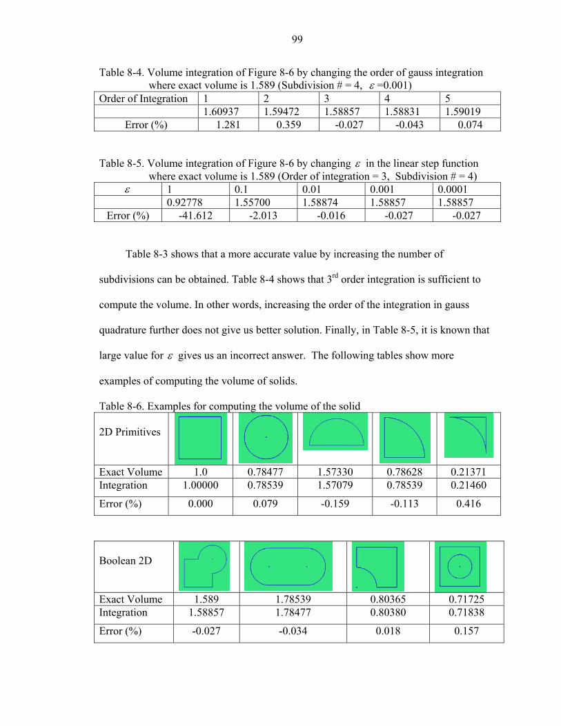
99
Table 8-4. Volume integration of Figure 8-6 by changing the order of gauss integration where exact volume is 1.589 (Subdivision # = 4, ε =0.001)
Order of Integration 1 2 3 4 5 1.60937 1.59472 1.58857 1.58831 1.59019
Error (%) 1.281 0.359 -0.027 -0.043 0.074
Table 8-5. Volume integration of Figure 8-6 by changing ε in the linear step function where exact volume is 1.589 (Order of integration = 3, Subdivision # = 4)
ε 1 0.1 0.01 0.001 0.0001 0.92778 1.55700 1.58874 1.58857 1.58857
Error (%) -41.612 -2.013 -0.016 -0.027 -0.027
Table 8-3 shows that a more accurate value by increasing the number of
subdivisions can be obtained. Table 8-4 shows that 3rd order integration is sufficient to
compute the volume. In other words, increasing the order of the integration in gauss
quadrature further does not give us better solution. Finally, in Table 8-5, it is known that
large value for ε gives us an incorrect answer. The following tables show more
examples of computing the volume of solids.
Table 8-6. Examples for computing the volume of the solid 2D Primitives
Exact Volume 1.0 0.78477 1.57330 0.78628 0.21371 Integration 1.00000 0.78539 1.57079 0.78539 0.21460
Error (%) 0.000 0.079 -0.159 -0.113 0.416
Boolean 2D
Exact Volume 1.589 1.78539 0.80365 0.71725 Integration 1.58857 1.78477 0.80380 0.71838
Error (%) -0.027 -0.034 0.018 0.157

100
3D Examples
Exact Volume 1.0 3.14159 0.58333 1.589 0.35862 Integration 1.00000 3.14159 0.58333 1.59852 0.35964 Error (%) 0.000 0.000 0.000 0.599 0.284
So far it has been only investigated the method to compute the volume of the solid
has been investigated. Surface area is another volumetric properties of the solid that
needs to be computed. One way of computing the surface areas is by summation of the
areas of triangles generated for graphical display of the solid. To compute the surface
area of the solid more systematically further research is needed.

CHAPTER 9 ALGORITHM FOR GRAPHICAL DISPLAY
To display the solid graphically it is necessary to polygonize or tessellate the
surface of the solid. Many algorithms have been developed [Bloomenthal, 1994], [Wyvill
and Overveld, 1997] for algebraic surfaces that can be easily adapted to generate
graphical display of primitives represented using implicit solid elements. An algorithm
has been developed that first tessellates the primitives and then uses these surface
triangles to construct the graphical display for the solid created by Boolean combination
of these primitives. The intersections between surface-triangles from different primitives
are computed followed by set membership classification to eliminate unnecessary
triangles. The details of this graphics algorithm are discussed in the following sections.
9.1 Overview of Computer Graphics
Even though there are the exact equations for curves in 2D and surfaces in 3D, their
computer graphics is displayed on the screen using lines and polygonal approximations.
Figure 9-1. Graphics of a curve
As shown in Figure 9-1, the graphics of a curve is composed of many line segments
where the number of line segments composing the curve determines the resolution of the
graphics. In other words, more line segments are required to obtain better graphics of the
101

102
curve. Such lines represented by two points need to be computed and stored for
displaying 2D graphics. Since this program is implemented by Java and Java3D, such
lines representing 2D graphics are stored in a class called LineArray.
Figure 9-2. Graphics of a sphere and its triangulation
Graphics for surfaces can be represented by any type of polygons such as triangles
or quadrilaterals. Figure 9-2 shows an example where a sphere is represented by many
triangles. As shown in Figure 9-2, the graphics of a surface is composed of many
triangles where the number of triangles composing the surface determines the resolution
of the graphics. The triangles are defined by three vertex points that need to be computed
and stored as arrays for displaying its 3D graphics. A class called TriangleArray is used
in Java3D for storing a triangulated approximation of surfaces for graphics display.
9.2 2D Primitive Display
Points on the boundary of the solid can be computed as intersection of rays from
the center of the element in general. A ray from the center in the direction
can be expressed as in the parametric space. The vectors n
r sˆ ˆn n i n= + j
unu ˆ)( =R r and ns are
expressed as cosine and sine of angle θ varying from 0 to 2π to evenly divide the space.

103
The intersection of this ray with the surface can be computed by solving the
equation
r s b(n u,n u) 0φ − φ = (9-1) Since the above equation is nonlinear, it has to be solved using Newton-Raphson
method in general (Point A in Figure 9-3). Note that the intersection of the ray and
boundary of the solid must be within the element. If no intersection of the ray and the
implicit Eq. 9-1 is found within the element then the intersection of the ray with the
boundary of the element needs to be found (Point B in Figure 9-3). The following figure
shows an example in the parametric space.
r
s
1
1
θ
bsr φφ =),(
)(uR
A
)(uR
B
Figure 9-3 Ray methods for finding points on the boundary of the solid in 2D
The LineArray for displaying the boundary of the solid in 2D is constructed by
connecting points computed by ray intersection with the boundary. Let a point on the
boundary of the solid be P(θ) which satisfies Eq. (9-1). Then the neighboring point can
be represented by P(θ+∆θ) where ∆θ is the step size of the angle increment. The
resolution of the 2D graphics depends on ∆θ. Therefore, smaller ∆θ must be used to
obtain higher resolution for the graphics of the 2D solid.

104
When the solid primitive to be displayed has an analytic equation, points on the
boundary can be found faster by directly using the analytic (parametric) equation of the
boundary. For quadrilaterals, the nodes of the element can be connected to form the
required line array. For an ellipse, the parametric coordinates of points on the boundary
of the ellipse can be easily computed using the equation
)sin,(cos),( ** θθ=sr Once the parametric coordinates of a point on the boundary are found, it
can be mapped to the global coordinates by the mapping function X(r, s).
),( ** sr
x
yr
s
1
1
)sin,(cos),( ** θθ=sr
θ
)sin,(cos),( ** θθXX =sr
Figure 9-4. Computing the points on the boundary of the ellipse
Even though all lines composing a 2D primitive can be saved in one LineArray,
they are separately listed in separate LineArrays where each LineArray represents each
edge in a 2D primitive. This is done for simplifying the algorithm to compute the
graphics for the Boolean result as described later in Section 9.5.
9.3 2D Boolean Result Display
At first in this algorithm for computing the LineArray to display the result of a 2D
Boolean operation, all the intersection points between the line segments of the base and
dependent solids are computed first. Thereafter the lines having intersections are divided
at these intersection points. This is based on the idea that the resultant geometry is

105
composed of lines divided at the intersections. Finally, set-membership classification is
applied to each divided line segment to determine line segments that are on the surface of
the Boolean result.
P (Intersection point)
B_v2
B_v3 B_v4
D_v1
D_v2
D_v3
D_v4
B_v1
B_v2B_v1 B_v2
B_v3B_v3B_v4
B_v4
PP
B_v1
D_v2D_v1 D_v2
D_v3D_v3D_v4
D_v4
PP
D_v1
Union
Dependent solid
Base solid
Figure 9-5. Union of two squares in 2D
As shown in Figure 9-5, the side B_v1-B_v4 in the base solid and the side D_v1-
D_v4 in the dependent solid are divided by the intersection point P. Therefore five line
segments each are obtained for the base and dependent solid. After applying set
membership classification on all line segments, the union result from the valid six line
segments is constructed.
The detailed procedure for 2D Boolean operation is explained in the following.
Input: n LineArrays from the base solid m LineArrays from the dependent solid
Output: LineArrays composing the Boolean solid 1. for i = 1 to n 2. if ith LineArray from the base solid intersects the bounding box of the dependent 3 solid element 4 then 5 for j =1 to m 6 for k = 1to number of lines composing ith LineArray 7 for l = 1 to number of lines composing jth LineArray 8 find intersection between two lines and save the intersection point 8 // end of l 9 // end of k 10 // end of j 12 else do set-membership classification on any line composing ith LineArray 11 if on the solid 12 then add ith LineArray for the Boolean solid

106
13 else discard ith LineArray 14 divide lines at the intersection points for ith LineArray 16 perform set-membership classification on each line 17 collect valid lines and make new LineArrays 18 // end of i 19 for j =1 to m 20 divide lines at intersection points for jth LineArray of the dependent solid 21 perform set-membership classification on each line segment of the array 22 collect valid lines and make new LineArrays 23 // end of j
As written in line 2 above, the bounding box method is used to check if an element
intersects another element. The bounding boxes are constructed by simply creating
rectangles by using the maximum and the minimum values in the nodal coordinates as
shown in the following figure.
solid element
Bounding box of the solidelement
x
y
Figure 9-6. Bounding box for a 2D solid element
Note that bounding box method only tells us that there is no intersection between
two solid elements when bounding boxes do not intersect each other. In other words, two
solid elements may not intersect each other even though their bounding boxes intersect
each other.
9.4 3D Primitive Display
There are two different algorithms for creating 3D primitive graphics depending on
whether the cross-section is constant or varying. For constant cross-sectional sweep, the

107
cross-section does not vary in the t direction. Therefore, points X(r*, s*, -1) on the
boundary of the 2D profile to be swept can be computed first and then similar points for
other t values as X(r*, s*, -1+j∆t) can be computed.
r
s
1
1 ),( ** srP
),,( ** tsrX
),,( ** tsrX
),,( ** tsrX
(A) (B)
(C) (D)
Figure 9-7. Computing the points on the boundary of the solid A) 2D profile to be swept B) Points on the extrude C) Points on the revolve D) Points on the sweep
As mentioned in section 9-1, TriangleArray is used for saving triangles where the
number of TriangleArrays for representing a 3D primitive depends on the number of
LineArray composing the 2D profile used.
For varying cross-sectional sweep, a more general method for finding points on the
boundary of the solid is needed. The points on the boundary of the solid can be computed
as the intersection of rays from the center of the cross-section. A ray from the center in
the direction can be expressed as r sn n= +n i j uu nR =)( in the parametric space. Similar

108
to 2D, nr and ns are expressed as cosine and sine of angle θ varying from 0 to 2π to
evenly divide the space.
The intersection of this ray with the surface can be computed by solving the
equation
0),,( * =− bsr tunun φφ (9-2) where, t* is the value of t at which points on the boundary are computed using this
ray algorithm. Since the above equation is nonlinear, it has to be solved using the
Newton-Raphson method in general.
Cross section where t = t*t=t*
r1
1
)(uR
θ
Figure 9-8. Finding the points on the boundary of the varying cross section sweep
After finding such points on the boundary of the solid for many evenly spaced
points in the t direction, these points are connected to construct the triangles needed to
display the 3D primitive solid.
9.5 3D Boolean Result Display
The triangle array to display the 3D Boolean result between the base and the
dependent solid is constructed directly from the triangle arrays of the base and dependent
solid. The elements of both base and dependent solid are first classified into intersecting
or non-intersecting elements so that only triangles of the intersecting elements need to be
investigated to find intersecting triangles thus simplifying the computation. After

109
computing all intersection between triangles to compute intersection points and lines, the
intersected triangles are sub-divided into smaller triangles by re-triangulating the vertices
and intersection points. Finally, set-membership classification is performed to classify all
triangles so as to collect all valid triangles that represent the Boolean result. The
procedure for computing the triangle array for the 3D Boolean result can be stated as the
following four steps.
Step1) Determine element to element intersection
Step2) Compute intersection points and lines from triangle to triangle intersection
Step3) Re-triangulate intersected triangles to include intersection points and lines
Step4) Perform set-membership classification to collect valid triangles
These steps are described in more detail below.
Step1) Determine element-element intersection
First of all, elements from base and dependent solids that intersect are determined
to minimize the total number of triangles that need to be searched to find intersections.
To obtain the benefit from this procedure, each triangle should be labeled so that the 3D
elements that contributed to creating the triangle can be determined. Before any Boolean
operations are performed each triangle is associated with a unique element. However,
during the Boolean operations if faces of two elements are coincident then after the
Boolean all the triangles on the coincident face are labeled as belonging to both the
elements. For each Boolean operation, only a few elements intersect each other, even
though the solids are composed of a lot of elements. Identifying the intersecting elements
will dramatically decrease the number of triangles that have to be search for possible

110
intersection. All 3D elements of the dependent solid are compared with all 3D elements
of the base solid in order to find intersecting elements.
Boolean solid Dependent
solid Base solid
Non-Intersected element node
Intersected element node
Figure 9-9. 3D CSG tree structure
Figure 9-9 shows a solid represented by a CSG tree where each 3D primitive node
is another binary tree. In other words, each 3D primitive is composed of one or more 3D
elements. Although the number of triangles for each solid is very large, the number of
triangles associated with the intersecting elements is much smaller. All TriangleArrays
associated with the intersecting elements are collected for the next step. Then set-
membership classification for non-intersecting triangle arrays is performed to determine
valid TriangleArrays among all non-intersecting TriangleArrays. If one of the triangles
from a TriangleArray is on the Boolean solid, the entire TriangleArray must be part of the
Boolean solid. Figure 9-9 illustrates the TriangleArrays of the base and dependent solid
as bars where each segment of the bar represents a triangle. The total number of
TriangleArrays of the base and the dependent solid are N and M respectively.
M dependent TriangleArraysN base TriangleArrays

111
Figure 9-10. All triangleArrays composing the base and dependent solid
To check whether two elements intersect bounding cylinder method is used. The
sweep trajectories connecting the centroids of the profile elements are defined for the two
elements of interest where sweep trajectory can be line in extrude, arc in revolve or
arbitrary curve in sweep. Thereafter, the closest points between the two trajectories are
computed as the optimal solutions obtained by minimizing )()( 21 tt SS − as shown in
Figure 9-10. Let D1 be the maximum diagonal at the 2D profiles used for creating
element 1and D2 be the maximum diagonal at the 2D profiles used for creating element
2. Then the minimum distance between two trajectories is compared with D1+D2 to
determine whether the bounding cylinders intersect. Let the minimum distance between
two trajectories be d, then
If d > D1+D2 bounding cylinders do not intersect
If d ≤ D1+D2 bounding cylinders intersect
Since bounding cylinder method is just an approximation, the bounding cylinder
method only tells us that there is no intersection between two solid elements when the
bounding cylinders do not intersect each other. In other words, two solid elements may
not intersect each other even though their bounding cylinders intersect each other.

112
Sweep trajectory(S1(t))
Closest points betweentwo trajectories
D1
D2
Sweep trajectory(S2(t))
Figure 9-11. Bounding cylinder method between two elements
Suppose the number of TriangleArrays from the intersected elements is n for the
base and m for the dependent, N-n TriangleArrays from the base and M-m
TriangleArrays from the dependent are either added to or removed from the Boolean
solid by the set-membership classification. Therefore, only n TriangleArrays from the
base solid and m TriangleArrays from the dependent solid will be considered in the
second step.
n base TriangleArrays m dependent TriangleArrays
Figure 9-12. All triangleArrays relevant to intersected elements
Step 2) Searching for intersection points and lines on triangles
As stated earlier, intersection between triangles that belong to the intersecting
elements is searched for now. Intersecting triangles may be coincident or intersecting
along a line. If two triangles are coincident, then intersection between edges of the

113
triangles to find “Edge-Edge” intersection points is searched for. On the other hand if the
triangles are intersecting but not coincident, then intersection between the edges of each
triangle with the other triangle is searched for to find “Plane-Edge” intersection point.
Representative examples of these two cases are shown in the following figure.
(B) (A)
Figure 9-13. Triangle-Triangle intersection A) Plane-Edge intersection B) Edge-Edge intersection
For each triangle, intersection points with edges of other triangles and intersection
lines with other triangles need to be stored so that they can be used for the next step of
the algorithm. Suppose the number of TriangleArrays having actually intersected
triangles is n* for the base and m* for the dependent, n-n* non-intersecting
TriangleArrays from the base and m-m* non-intersecting TriangleArrays from the
dependent are either added to or removed from the graphics by performing set-
membership classification. Therefore, only n* TriangleArrays from the base solid and m*
TriangleArrays from the dependent solid will be considered in the third step.
n* base TriangleArrays m* dependent TriangleArrays
Non-intersected triangle
Intersected triangle
Figure 9-14. TriangleArrays having actually intersected triangles

114
Step3) Triangulation
Different types of triangulation procedures are used to handle the coincident and
intersecting triangles. If the two or more triangles are coincident, all these triangles will
be simultaneously triangulated. On the other hand intersecting triangle are triangulated
individually. The well known Delaunay triangulation algorithm with some minor
modifications is used in this system. Since Delaunay triangulation algorithm works for
points on a plane, a mapping procedure to transform points in 3D to points in 2D is
needed. This mapping is described below.
P Pu
w v
V3
V1 V2 V2
V3
V1
v
y
z
u
x
Figure 9-15. Mapping the triangle in space onto the local u-v plane
In Figure 9-14, u is a unit vector connecting V1 to V2. w is the unit vector which is
normal to the triangle. Then v can be computed by
v=w×u Let a point P be a given point on the triangle. Its coordinates (u, v) with respect to a
local 2D coordinates system is computed as
u = d cosθ v = d sinθ
where d = distance from the V1 to P
θ = angle between u and the vector V1-P
Once all points are mapped to u-v plane, those points are used for the Delaunay
triangulation. The swap procedure in the triangulation algorithm is modified to make sure
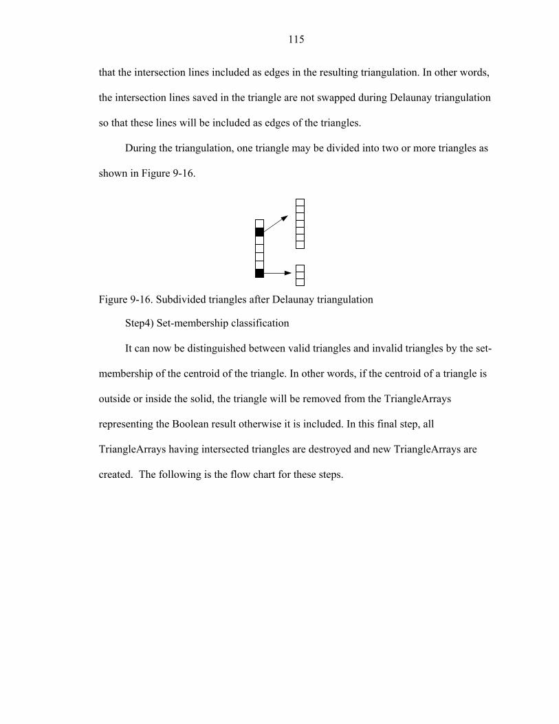
115
that the intersection lines included as edges in the resulting triangulation. In other words,
the intersection lines saved in the triangle are not swapped during Delaunay triangulation
so that these lines will be included as edges of the triangles.
During the triangulation, one triangle may be divided into two or more triangles as
shown in Figure 9-16.
Figure 9-16. Subdivided triangles after Delaunay triangulation
Step4) Set-membership classification
It can now be distinguished between valid triangles and invalid triangles by the set-
membership of the centroid of the triangle. In other words, if the centroid of a triangle is
outside or inside the solid, the triangle will be removed from the TriangleArrays
representing the Boolean result otherwise it is included. In this final step, all
TriangleArrays having intersected triangles are destroyed and new TriangleArrays are
created. The following is the flow chart for these steps.

116
Task 3:
Task 2:
Task 1:
Triangulation for each triangle
Triangulation for all coincident planes simultaneously
Set-membership classification on N-n non-intersected base TriangleArrays M-m non-intersected base TriangleArrays Collect valid TriangleArrays and add to the Boolean solid
End
Set-membership classification Collect valid triangles and create new TriangleArrays which will be added to the Boolean solid
Finding intersections on all intersected triangles
Element-Element Intersection n intersected base TriangleArrays m intersected dependent TriangleArrays
No
Yes
N base TriangleArrays M dependent TriangleArrays
Start
Coincident cases exist
Task 4:
Figure 9-17. Flow chart for constructing the graphics for the 3D Boolean result
9.6 Discussions and Suggestion for improvement
The method used for displaying the graphics of the solids in this system is not very
efficient and needs to be improved to obtain better display speed. There are many reasons
for the inefficiency of the algorithm.
Currently an iterative numerical method is used find points on the boundary of the
primitives. This cannot be avoided if the equation representing the intersection of a ray
and the boundary is a high degree nonlinear equation. Using analytical solution whenever
possible instead of numerical method, can significantly improve the graphics display
117
speed. Set membership classification needs to be performed repeatedly during the
procedure to classify a very large number of triangles. Better algorithms for determining
element to element intersection, element to triangle array intersection or triangle to
element intersection can reduce the number of triangles whose intersections need to be
computed.

CHAPTER 10 CONCLUSION AND DISCUSSION
10.1 Conclusion
In this study, an approach for representing primitive solids using implicit solid
elements is presented. These primitives can be combined using Boolean operation to
create more complex solids. In traditional CSG approach the primitives are defined by
Boolean combination of half-spaces. Instead, in this approach, the primitives are defined
using implicit surface functions that are represented parametrically within quadrilateral or
hexahedral elements. By representing the density function parametrically, many of the
advantages of parametric curve and surface representation such as axes independence and
ease of tracing are inherited by the implicit solid element representation. A primitive
represented using implicit solid element can be edited by changing the nodal density
values, level set value ( bφ ) or by changing the size of the element.
The implicit solid elements introduced in this study enable the representation of
sweep solids using implicit surface boundaries. The solid elements for representing
sweep solids are classified by the type of sweep trajectory as well as by the cross-section
shapes. Implicit solid elements were developed for each type of sweep solid including
extrude, revolve and general sweep. In general the biggest draw back of implicit surface
representation is that it is necessary to solve equations to compute points on the
boundaries of the solid. However, when the implicit surface functions are defined within
quadrilateral and hexahedral elements that are not distorted, fairly simple algorithms can
be developed for generating tesellations required for graphical display. The main
118

119
advantage is that set membership classification is easier for implicit solid elements
compared to B-Rep models especially when the elements are not distorted. Another
advantage is that Boundary evaluation algorithms are not required when the solid is
represented using either implicit half spaces (as in conventional CSG technique) or when
implicit solid elements are used to define the primitives.
Furthermore when the implicit solid elements are used for representing the solids
additional information such as material properties can be super-impose by assigning
nodal values for these properties. The variation of these properties within the solid can be
represented using appropriate interpolation within the element. If necessary, the element
can be sub-divided into smaller elements to provide the necessary resolution to represent
material variation required to represent any type of heterogeneous solids. The algorithms
presented in this study are implemented using Java and Java3D to verify the algorithms
and to compare performance with B-Rep models.
10.2 Future Work
Since this approach is just introduced, there are still many problems to be solved. It
is required to develop implicit solid elements for freeform modeling as well as for
representing other types of features routinely used in current CAD systems. And most
solid models can be used for FEA (Finite Element Analysis) after generating meshes on
them and for finding NC tool path for manufacturing. To establish such abilities in this
solid modeling system, further study is needed. Without developing these techniques
implicit solid modeling is unlikely to be a viable alternative to the currently popular B-
Rep technology.

APPENDIX SCENEGRAPH AND CLASS STRUCTURE
A.1 SceneGraph Structure for Java3D
Locale
Base Solid Dependent Solid
BranchGroup(BG)
TransformGroup(TG)
BG
Face Edge Vertex Mesh Node FlipArrowDimensionLine
Dimension
RefEdgeRefFace RefVertex
BGBG
TG
PickTranslate PickRotate PickZoom
ViewModel
MousePick
Figure A-1 SceneGraph structure for the solid modeler using implicit solid elements
120

121
A.2 SDModeler Classes
Class structure Packages
commandList constraint delauny equationSolver graphicsComponent interactiveCommand shapedensity solidModel userInterface
Main Class : SDModeler
commandList
ClAssembly ClBoolean ClEdit ClFile ClHelp ClMain ClSelect ClSolid2D ClSolid3D ClView
delauney
Dtriangle
constraint
ConstraintSet PositionConstraint Utility VL_C VL_D VP_D VV_A VV_C VV_D VV_P
graphicsComponent
Curve CurveHermite DimensionText2D Line PickPoint PickPtElementNode PickPtIntersection PickPtstatic PickVector SdLineArray SdPointArray SdTriangleArray Triangle UtilGeometry
equationSolver
CCNewtonRaphson CLNewtonRaphson EquationSolver
InteractiveCommand IcAlignLines IcDimensionChange IcExtrude IcRevolve IcSolid2DPrimitives IcVLC IcVLD IcVPD IcVVA IcVVC IcVVD IcVVP InteractiveCommand
shapedensity
Q4Node Q8Node Q9Node Sd3DExtrude Sd3DRevolve Sd3DSMBlend Sd3DSTBlend Sd3DSweep ShapeDensity ShapeDensity2D ShapeDensity3D T10Node
solidModel
CSG_History Constraints CsgNode Solid Solid2D Solid2dCircle Solid2dEllipse Solid2dRectangle Solid2dTriangle Solid2dSemiCircle Solid2dQuaterCircle Solid2dWedge Solid3D Solid3dExtrude Solid3dRevolve Solid3dSMBlend Solid3dSTBlend Solid3dSweep
userInterface
FileIO Java3DUniverse MainDialogBoxes MousePick SDModelerFrame ViewCanvas

122
A.3 SDModeler Class Structure
ViewCanvas
Solid
CSG_History
CsgNode
Java3DUniverseSDModelerFrame
CommandList
JFrame
SDModeler
Canvas3D
Constraints
ShapeDensity
Solid2D Solid3D
Solid2dCircle Solid2dEllipse
Solid2dRectangle
Solid3dExtrude Solid3dSweep
InteractiveCommand
Solid3dRevolve
Solid3dSweepSTBlend
Solid3dSweepSMBlendSolid3dSTBlend
Solid3dSMBlend
Solid2dSemiCircle
Solid2dQuaterCircle Solid2dTriangle
Solid2dWedge
Figure A-2 Class structure for the solid modeler using implicit solid elements
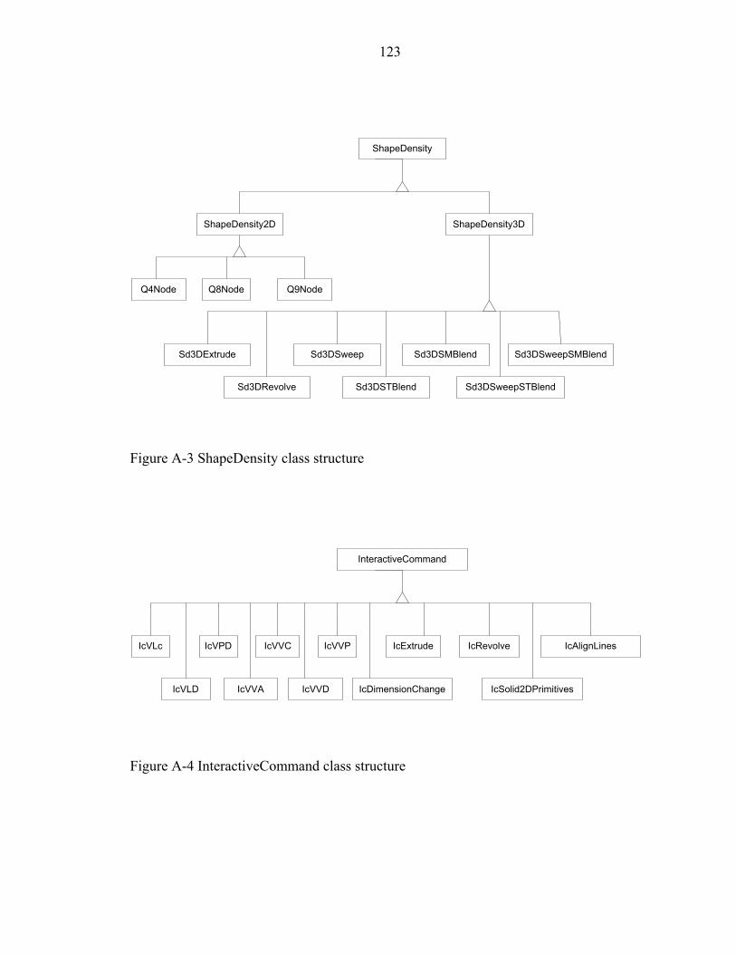
123
ShapeDensity2D
ShapeDensity
ShapeDensity3D
Q4Node Q8Node Q9Node
Sd3DExtrude
Sd3DRevolve
Sd3DSweep
Sd3DSTBlend
Sd3DSMBlend
Sd3DSweepSTBlend
Sd3DSweepSMBlend
Figure A-3 ShapeDensity class structure
InteractiveCommand
IcExtrudeIcVLc
IcVLD
IcVPD
IcVVA
IcVVC
IcVVD
IcVVP
IcDimensionChange
IcRevolve
IcSolid2DPrimitives
IcAlignLines
Figure A-4 InteractiveCommand class structure

124
CommandList
ClSolid3DClAssembly
ClBoolean
ClEdit
ClFile
ClHelp
ClMain
ClSelect
ClSollid2D ClView
Figure A-5 CommandList class structure
ConstraintSet
VP_DVP_D VP_DVP_DVP_DVL_D VL_C
PositionConstraint Figure A-6 PositionConstraint class structure

LIST OF REFERENCES
Bajaj C, Chandrajit L, Chen J and Xu G, 1995, Modeling with Cubic A-Patches, ACM Transactions on Graphics, 14(2), pp.103-133.
Bloomenthal, J., 1994, An Implicit Surface Polygonizer, Graphics Gems IV, New York, Academic Press.
Bloomenthal J, Bajaj C, Blinn J, Cani-Gascuel MP, Rockwood A, Wyvill B and Wywill G, 1997, Introduction to Implicit Surfaces, Morgan Kaufmann Publisher Inc, San Francisco, CA.
Choi B.K. and Lee C.S., 1990, Sweep Surfaces Modeling via Coordinate Transformations and Blending. Computer-Aided Design, 22:87-96.
Filip, D. J.and Ball, T. W., 1989, Procedurally Representing Lofted surfaces, IEEE Computer Graphics and Applications v 9 n6 p 27-33.
Glassener A, 1989, An Introduction to Ray Tracing, Academic Press, London.
Hoffmann C, 1987, Geometric and Solid Modeling-An Introduction, Morgan Kaufmann Publishers, San Mateo, CA.
Kumar, A. V. and Gossard D. C., 1996, Synthesis of Optimal Shape and Topology of Structures, Journal of Mechanical Design, Transaction of the ASME, vol. 118, no. 1, pp. 68.
Kumar, A. V. and Yu, L., 2001, Sequential Constraint Imposition for Dimension-Driven Solid Models, Computer Aided Design, 33(6), pp. 475-486.
Lee K, 1999, Principles of CAD/CAM/CAE System, Addison Wesley, Reading, MA.
Lorensen W. and Cline H., 1987, Marching Cubes-A High Resolution 3D Surface Construction Algorithm, Computer Graphics, 21(4), pp.163-69.
Mantyla M, 1988, An Introduction of Solid Modeling, Computer Science Press, Rockville, MD.
Tigges M. and Wyvill B., 1999, A Field Interpolated Texture Mapping Algorithm for Skeletal Implicit Surfaces, Proceedings of Computer Graphics International, Canmore, Canada.
125

126
Martin R.R. and Stephenson, 1990, P.C. Sweeping of Three-Dimensional Objects. Computer-Aided Design , 22:223-234.
Mortenson ME, 1997, Geometric Modeling Second Edition, Wiley Computer Publishing, John Wiley and Sons, New York.
Osher S. and Redkiw R., 2003, Level Set Methods and Dynamic Implicit Surfaces, Springer-Verlag Inc., New York
Requicha, AAG and Voelcker HB, 1985, Boolean Operations in Solid Modeling: Boundary Evaluation and Merging Algorithms, Proceedings of the IEEE, 73(2), pp. 30-40.
Shapiro V., 1998, Theory of R-functions and Applications: A Primer. CPA Technical Report CPA88-3, Cornell Programmable Automation, Sibley School of Mechanical Engineering, Ithaca, NY 14853.
Shapiro V. and Tsukanov, 1999, Meshfree Simulation of Deforming Domains, Computer-Aided Design, 31, pp. 459-471.
Spatial Technology Inc., 1995, Geometry Modeler Application Guide, Spatial Technology Inc., Boulder, CO.
Wyvill, B. and Overveld, K. V., 1997, Polygonization of Implicit Surfaces with Constructive Solid Geometry, J. of Shape Modeling, 2(4), pp. 257-273.
Zeid I.,1991, CAD/CAM Theory and Practice. McG Computer Science Series, Singapore.
Zhao HK, Osher S, Merriman B and Kang M, 2000, Implicit and NonParametric Shape Reconstruction from Unorganized Data Using a Variational Level Set Method, Computer Vision and Image Understanding, 80, pp.295-314

BIOGRAPHICAL SKETCH
The author was born on September 6, 1970, in Seoul, Korea. In 1996, he graduated
with a Bachelor of Science degree in mechanical engineering from Inha University,
Inchon, Korea. He entered the Master of Science program in the Mechanical Engineering
Department at the University of Florida in 1997 and obtained his master’s degree in
1998. Thereafter he continued to study in the Ph.D. program.
On November 23, 1996, he was married to Duyoung Kim. He is the father of two
lovely daughters, Jasmine and Anna.
127