Solid State Physics

Study Support

Prof. RNDr.Pavel Koštial,CSc.

Ostrava 2015

VYSOKÁ ŠKOLA BÁŇSKÁ – TECHNICKÁ UNIVERZITA OSTRAVA

FAKULTA METALURGIE A MATERIÁLOVÉHO INŽENÝRSTVÍ

1

Title:Solid State Physics

Code:

Author: Prof. RNDr. Pavel Koštial,CSc.

Edition: first, 2015

Number of pages: 76

Academic materials for the Advanced Engineering Materials study programme at the

Faculty of Metallurgy and Materials Engineering.

Proofreading has not been performed.

Execution: VŠB - Technical University of Ostrava

2

STUDY INSTRUCTIONS

This text serves as the basic orientation material for the study of the subject Physics of

Solids for the second stage of higher education. It is an overview of the concepts of the

subject of study, but it is not a classic textbook. The material is also varied with a series of

images that should make them more legible. For a deeper understanding is needed, however,

to resort to classical textbooks .

The subject is included in the master's study and study support is divided into parts,

chapters, which correspond logically divided the study drug but not equally extensive.

Estimated time to study chapters can vary widely, so are large chapters further divided into

numbered subsections and answers them structure described below. The material is suitable

for students with a focus on material engineering, diagnostics of materials, chemistry, as well

as other interested parties of technical fields.

At the outset, this chapter is given the time needed to study the substance. Time is only

indicative.. Further such goals are to be achieved student after studying this chapter and

specific knowledge. Followed by the interpretation of the study material, the introduction of

new concepts, explanations, all of which is accompanied by images and tablesi.At the end of

each chapter are repeated the main concepts.. To verify fully mastered the material chapter, a

student at the and of every chapeter have of several theoretical questions.

Communication

Prof. RNDr.Pavel Koštial, CSc..

email: pavel.kostial@vsb.cz

tel. +420597324498

3

CONTENT

1. Tensors 4

1.1 Transformation of coordinates 4-13

1.2 Properties of tensors 13-17

1.3 Stress tensor 17-20

1.4 Strain tensor 20-23

1.5 Elastic constants tensor 23-25

1.6 Compressibility 25

1.7 Impact of lattice symmetry on tensor representation 26-30

2.The basics of statistical physics

and quantum mechanics 32

2.1 Statistical interpretation of a physical systems

description with many particles 32-36

2.2 The basics of wave particle description 37-39

2.3 Quantum statistics 39-43

2.4 Schrodinger equation 43-44

2.5 The phace space 45-46

3. Viscous and viscous-elastic behaviourof materials 48

3.1 Charasteristics of viscous and

viscous elastic materials 49-63

3.2 Models of viscous elastics materials 63-70

3.3 Payne effect 70-74

4

1 Tensors

Study time 5 hours

Objectives

you will be familiar with the tensor description of the anisotropic properties of

materials

you will learn about the basis of tensors number in applications on materials

you will learn about calculations of specific physical quantities in anisotropic

materials

you will understand the relationship between the structure of material and its

mathematical description

LLecture

1.1.Transformation of coordinates

The term mass point, whose position in space is determined by the position

vector r , is one of the fundamental concepts of classical mechanics. The first

derivation of the position vector by time determines the velocity, and the second

derivation the mass point acceleration.

In the case of an N system of mass points the number of coordinates

determining the position of such a system is equal to 3N . If the mass points are

independent, then the number of degrees of freedom is also 3N .

From the elementary course on physics we know that the mass point

position is always determined with regard to a selected reference system. This

system allows us to describe the mass point position in general N with

5

independent variables qi, (i=1, 2, ..N), which characterise the system position with

N degrees of freedom, and we call them generalized coordinates.

Their first derivation by time we call generalized velocity and the second

derivation generalized acceleration..

The full determination of such a mechanical system requires to know N

number of generalized coordinates and N number of generalized velocities.

A good example of such generalized coordinates can be illustrated by the

polar coordinates r and , suitable e.g. to describe a mass point movement on a

circle.

Movement of the mechanical system is determined by kinetic equations,

such as the differential relations between coordinates and velocities. Motion

equations, expressed in generalized coordinates, have also generalized forms.

From the elementary physics course we know that we can distinguish scalar

physical quantities (also called zero-order tensors), which are fully

determined by entering numbers (scalar values), which are independent of

coordinate system selection. This can be described mathematically in a three

dimensional space using the scalar function of coordinates f(x 1 , x 2 , x 3 ), which is

invariant against the coordinate axes transformations, and so it holds that f(x 1 , x 2

, x 3 ) = f(x 1 ', x 2 x 3 ', '). These include physical quantities such as mass, density,

temperature, and more.

In contrast to them, there are also vector quantities (also called tensors of the

first order). If we identify a suitable coordinate system, which is dependant on

transformation rules (see relations in 1.13, 1.14), then the vector is fully

determined by entering its components´ values in the direction of these coordinate

axes.

Thus, we understand the vector also as an ordered triple system (in a

general n-th system) of the scalar values - vector coordinates in the selected

coordinate system. Among vector physical quantities belong acceleration, force,

etc.

6

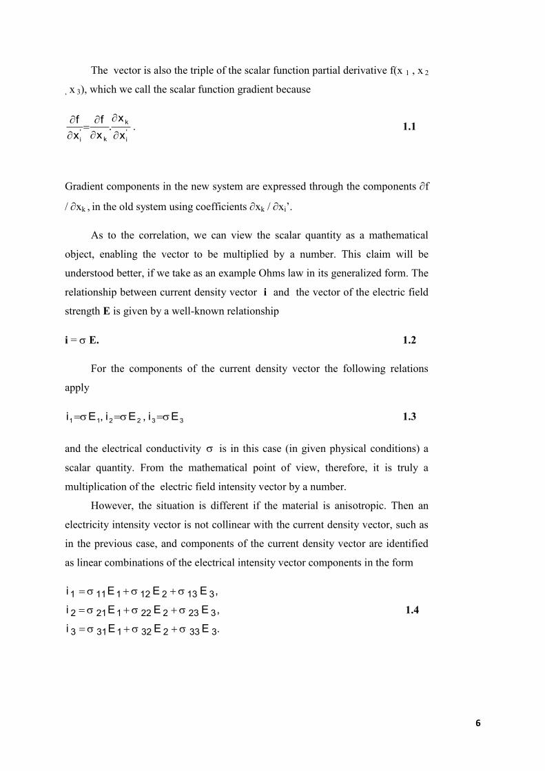
The vector is also the triple of the scalar function partial derivative f(x 1 , x 2

, x 3), which we call the scalar function gradient because

'

i

k

k'

i x

x.

x

f

x

f

. 1.1

Gradient components in the new system are expressed through the components f

/ xk , in the old system using coefficients xk / xi’.

As to the correlation, we can view the scalar quantity as a mathematical

object, enabling the vector to be multiplied by a number. This claim will be

understood better, if we take as an example Ohms law in its generalized form. The

relationship between current density vector i and the vector of the electric field

strength E is given by a well-known relationship

i = E. 1.2

For the components of the current density vector the following relations

apply

332211 Ei,Ei,Ei 1.3

and the electrical conductivity is in this case (in given physical conditions) a

scalar quantity. From the mathematical point of view, therefore, it is truly a

multiplication of the electric field intensity vector by a number.

However, the situation is different if the material is anisotropic. Then an

electricity intensity vector is not collinear with the current density vector, such as

in the previous case, and components of the current density vector are identified

as linear combinations of the electrical intensity vector components in the form

i E E E

i E E E

i E E E

1 11 1 12 2 13 3

2 21 1 22 2 23 3

3 31 1 32 2 33 3

,

,

.

1.4

7

It is clear that the electrical conductivity is no longer a scalar quantity, but

each of the values ij has its specific physical importance.

If the electric field is applied in the direction of the axis x 1 , then the vector

of the electric field intensity components are

E = (E 1 , 0.0) 1.5

and the current density vector will include

131312121111 Ei;Ei;Ei . 1.6

Importance of the current density vector components can be seen in Figure 1.1.

Figure 1.1. Importance of the current density vector components

Thus, the electrical conductivity in the case of an anisotropic crystalline material

is generally determined by nine independent components, which form the tensor

of the second order (named after the number of components indices), which can

be written in the form of a matrix

11 12 13

21 22 23

31 32 33

. 1.7

8

The second order tensor may be seen as a mathematical object

(operator), which clearly defines the relation between the two vector

quantities.

Later, we will demonstrate that the fourth order tensor is determined by the

functional relationship between two tensors of the second order.

Equation 1.3, which illustrates the dependence of the current density vector on the

electric field intensity vector, can also be written in the reduced form

32,1,i,32,1,j,Ei3

1j

jiji

1.8

or

,3,2,1j,iEi jiji 1.9

while we have used the so-called Einstein summation convention, under which

we always add up following the index, which is repeated twice. In this case, it is

the index j, which we call the summational index . Index i is called the free

index.

Many times, when solving physical tasks, we are confronted with the

problem that it is necessary to pass from one coordinate system (related, for

example, to the crystallographic orientation) to the coordinate system of work, in

which the task is solved (e.g. the dynamics of the elastic waves propagation in the

crystal, in a specified direction, and in a given plane). We will try to explain some

parts of these interesting problems here.

Before we proceed to study the issue of transformations, let us define one

general rule, which must be met, regardless of what type of transformation we are

dealing with.

9

In the transition (transformation) from one coordinate system to

another, only the form of the transformed quantity notation changes, but not

the transformed quantity itself .

To keep this rule, it is necessary to define the transformation rules, which

will be based on Figure 1. 2.

For transforming coordinate axes we will assume that both systems have a

common origin. Relations between the "old" and "new" axes are determined by

a table (matrix)

"the old axis" 1.10

"the new axis"

333231

232221

131211

aaa

aaa

aaa

The first index in the matrix refers to the 'new' axes and the second one to the

"old" axes.

10

Figure 1.2. Transformation of the coordinate axes

Note .

From transformation theory we know that the so-called relations orthogonality

must be met, from which the first can be written in the form (the sum of

squares for direction cosine equals to one)

.1aaa

,1aaa

,1aaa

2

33

2

32

2

31

2

23

2

22

2

21

2

13

2

12

2

11

In the reduced form these equations can be expressed as 1aa jkik for i=j.

The second condition (orthogonality ) is met if the equation

.0aaaaaa

,0aaaaaa

,0aaaaaa

231322122111

133312321131

332332223121

Reduced notation of these equations will be 0aa jkik for ji .

11

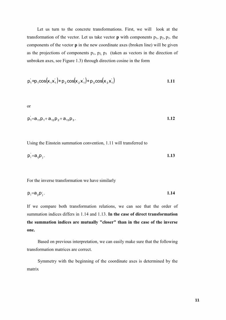
Let us turn to the concrete transformations. First, we will look at the

transformation of the vector. Let us take vector p with components p1, p2, p3. the

components of the vector p in the new coordinate axes (broken line) will be given

as the projections of components p1, p2, p3 (taken as vectors in the direction of

unbroken axes, see Figure 1.3) through direction cosine in the form

( ) ( ) ( )'133

'

122

'

111

'

1 xxcosp+xxcosp+xxcosp=p 1.11

or

313212111

'

1 papapap . 1.12

Using the Einstein summation convention, 1.11 will transferred to

jij

'

i pap . 1.13

For the inverse transformation we have similarly

,

jiji pap . 1.14

If we compare both transformation relations, we can see that the order of

summation indices differs in 1.14 and 1.13. In the case of direct transformation

the summation indices are mutually "closer" than in the case of the inverse

one.

Based on previous interpretation, we can easily make sure that the following

transformation matrices are correct.

Symmetry with the beginning of the coordinate axes is determined by the

matrix

12

100

010

001

SS . 1.15

From the plane of symmetry perpendicular to the axis x 3 the following

applies

100

010

001

3XM . 1.16

The coordinate system rotations by the angle 2 / 3 about the diagonal dice

is determined by matrix

001

100

010

32;111 . 1.17

For the torsion of an angle around axes x 1 and x 2 these transformation

matrices should have the form

cossin0

sincos0

001

;x1 1.18

and

cos0sin

010

sin0cos

;x 2.

13

Figure 1.3. Transformation of the vector

1.2. Properties of tensors

In the previous section we have dealt with the issues of zero-order tensors

(scalars) and the first order (vectors). In this section we will deal with tensors of

higher-orders and the mathematical apparatus, which describes them. First, we

will examine transformation relations applicable to tensors of higher-orders. The

transformation of a tensor (let us see it as a mathematical object enabling the

functional relationship between two vectors) will be explained on a general

example, using the vectors of effect u and the causes p. We will proceed

following the scheme

u’ u p p’. 1.19

Then we gradually get

kik

'

i uau . 1.20

If we use k as a free index and l as a summation index, then, in accordance with

I.13, we get

.pT=u lklk 1.21

By analogy, we replace the summation index l for the free now, and we have

'

jjll pap 1.22

14

or

.paTapTauau '

jjlkliklklikkik

'

i 1.23

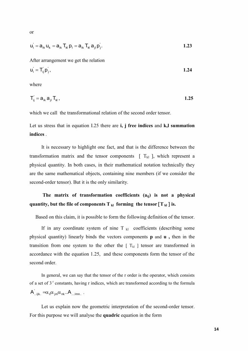
After arrangement we get the relation

'

j

'

ij

'

i pTu , 1.24

where

kljlik

'

ij TaaT , 1.25

which we call the transformational relation of the second order tensor.

Let us stress that in equation I.25 there are i, j free indices and k,l summation

indices .

It is necessary to highlight one fact, and that is the difference between the

transformation matrix and the tensor components Tkl , which represent a

physical quantity. In both cases, in their mathematical notation technically they

are the same mathematical objects, containing nine members (if we consider the

second-order tensor). But it is the only similarity.

The matrix of transformation coefficients (aij) is not a physical

quantity, but the file of components T kl forming the tensor T kl is.

Based on this claim, it is possible to form the following definition of the tensor.

If in any coordinate system of nine T kl coefficients (describing some

physical quantity) linearly binds the vectors components p and u , then in the

transition from one system to the other the [ Tkl ] tensor are transformed in

accordance with the equation 1.25, and these components form the tensor of the

second order.

In general, we can say that the tensor of the r order is the operator, which consists

of a set of 3 r constants, having r indices, which are transformed according to the formula

....lmn..

'

...ijk.. AA ..nkjmil .

Let us explain now the geometric interpretation of the second-order tensor.

For this purpose we will analyse the quadric equation in the form

15

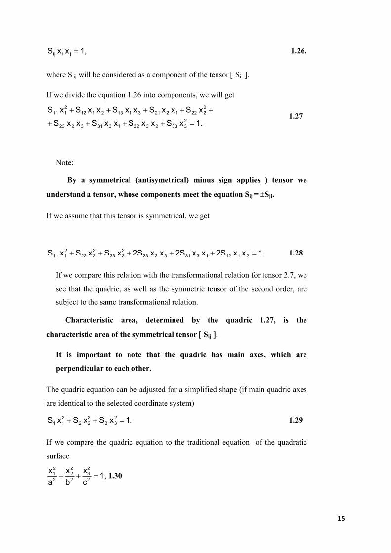
1xxS jiij , 1.26.

where S ij will be considered as a component of the tensor Sij .

If we divide the equation 1.26 into components, we will get

.1xSxxSxxSxxS

xSxxSxxSxxSxS

2

333233213313223

2

222122131132112

2

111

1.27

Note:

By a symmetrical (antisymetrical) minus sign applies ) tensor we

understand a tensor, whose components meet the equation Sij = Sji.

If we assume that this tensor is symmetrical, we get

.1xxS2xxS2xxS2xSxSxS 211213313223

2

333

2

222

2

111 1.28

If we compare this relation with the transformational relation for tensor 2.7, we

see that the quadric, as well as the symmetric tensor of the second order, are

subject to the same transformational relation.

Characteristic area, determined by the quadric 1.27, is the

characteristic area of the symmetrical tensor Sij .

It is important to note that the quadric has main axes, which are

perpendicular to each other.

The quadric equation can be adjusted for a simplified shape (if main quadric axes

are identical to the selected coordinate system)

.1xSxSxS 2

33

2

22

2

11 1.29

If we compare the quadric equation to the traditional equation of the quadratic

surface

1c

x

b

x

a

x2

2

3

2

2

2

2

2

1 , 1.30

16

we are getting for the main half axes the values

,S

1,

S

1,

S

1

321

1.31

where S i are diagonal components of the tensor Sij .

If all the components of the Si are positive, then the characteristic surface is an

ellipsoid. If there are two coefficients positive and one negative, the area is a uni-

axial hyperboloid. If there are two coefficients negative and one positive, the

characteristic area is two axial hyperboloids (see Figure 1.4).

Figure 1.4. Ellipsoid (a), uni-axial hyperboloid (b), two axial

hyperboloids(c)

.0S ijij 1.32

i j is Kronecker's symbol. Three roots define the main axes of the characteristic

surface and it can be demonstrated that all the three main axes are mutually

orthogonal, and that the following ’= S1, ’’= S2, ’’’= S3 applies.

Quantities are also called eigenvalues of tensor Sij .

The sum of the eigenvalues of tensor Sij is its invariant.

17

Vectors determined by the equation 1.33 are called the eigenvalues of tensor

Sij . Eigenvalues of the tensor Sij are real values and the directions

determined by these values are mutually orthogonal.

From a practical point of view, we often need to determine the value of the

tensor variable in a given direction. For this problem solving, depending on the

coordinate system we recognize two cases, which again we will demonstrate

using the electrical conductivity of a tensor.

1.Let the direction cosines 3,21 ll,l determine the selected direction of

electrical conductivity. If the electric field is oriented in this direction, then we

can express it using the form El,El,ElE 321 . Then for a current density applies

El,El,Eli 332211 . The component of the current density projected in the E

direction will be ElElEli 3

2

32

2

21

2

1 . Then the electrical conductivity in

direction li will be 3

2

32

2

21

2

1 lll .

2. Let the coordinate system be oriented arbitrarily toward the main axes of

the electrical conductivity tensor.

If we have direction cosines li with an arbitrary coordinate system, so it is

ii l.EE . The component of the current density i in the direction E will be E/Ei

or written as tensor E

Ei ii . For the electrical conductivity we get

2

ijij

2

ii

E

EE

E

Ei , or jiij ll .

1.3. Stress tensor

We have understood these forces tacitly as the "point effect". In fact, real

forces operate within a certain area, and thus we no longer talk about the power,

but about the mechanical stress that causes distortion. In the basic course of

physics you have already analysed these terms, but for an isotropic body.

It was stated that the "mechanical stress is homogeneous throughout the

whole body", "all its particles are statistically balanced", "volume powers and

18

volume moments are negligible". Now we will broaden our knowledge with a

comprehensive view of the issue.

We will follow the Figure 1.5 with the unit cube.

Figure 1.5. Distribution of stress in a homogeneously tensed solid matter.

From this picture it is clear that the components of tensor distortions [Tij]

are positive in the case of stresses causing dilatation to a solid body, and negative,

if these tensions cause any contraction. It is also clear that the diagonal

components of the stress tensor T 11, T 22, T 33 represent normal stress components,

and components T ij for i j are tangential components.

But let us return to the definition of the mechanical stress concept. We will use

Figure I. 6.

On the surface of S2, which normally is parallel to the x2 axis, the stresses T12,

T22, T32 operate , where e.g. T12 is defined by the relation

2

1

0S12

S

FlimT2

1.33

or generally

k

i

0Sik

S

FlimTk

. 1.34

19

Figure 1.6. Definition of mechanical stress. Element of the surface is

perpendicular to the coordinate axis (a). Arbitrarily oriented element

of the area (b).

T ik represents the i –th component of a force applied to the surface

perpendicular to the axis xk . Perhaps its environment, based on the law of action

and reaction, will act with an equally large, but reversed force.

In conclusion, here are some special cases of the stress tensor. For uniaxial

tension the stress tensor is in the form

T11 0 0

0 0 0

0 0 0

. 1.35

For the two axes stress there will apply

T

T

11

22

0 0

0 0

0 0 0

. 1.36

"Pure" shear stress will be expressed in the form

20

0 0

0 0

0 0 0

12

12

T

T

. 1.37

Hydrostatic pressure p shall be expressed by the matrix

p

p

p

0 0

0 0

0 0

. 1.38

1.4. Strain tensor

Strain tensor describes the "response" of a solid body to the stress

operation. In this section, we will analyse also other processes in connection

with the changes of the body dimensions, such as e.g. thermal expansion. We

shall start with the already known Figure 1.7 , which describes the deformation of

a "unilaterally fixed" bar oriented in the direction of the F force.

If we take on this rod a length piece with the M and N end points, which

Figure 1. 7. Deformation of this "unilaterally fixed" rod under the influence

of the F force

have the coordinates x and x + x, then after the deformation influenced by F

force we will get

21

the new coordinates of the mentioned point in the form of x + u(x) and x + x +

u(x +x), where u(x) is the connected function of coordinates.

Relative elongation of the MN element is then defined in the vicinity of the

M point (i.e. for x 0) by the first derivative as per x in the form

dx

du

x

ulime

0x

. 1.39

Let us stress that distortion is a dimensionless value . From the above

mentioned explanation it is clear that the influence of the F force should cause

only the linear deformation (the motion of atoms in the direction of the force

operation), if we do not consider changing the diameter of the bar used.

But the reality is more complicated and here is no physical reason for the

real material to act in such a way. The movement of atoms is dependent inter alia

also on the crystallographic system and, therefore, also on the type of chemical

bonds operating among atoms.

Strain tensor can be expressed using the relation

j

k

i

k

i

j

j

iij

x

u

x

u

x

u

x

u

2

1S , 1.40

Nine constituents Sij form the second-order tensor [Sij], which we call the strain

tensor.

Most of them are small deformations and the following applies

i

j

i

iij

x

u

x

u

2

1S , 1.41

While we have neglected the second-order expression

j

k

i

k

x

u

x

u

1.42

This approximation then leads to the so-called linear elastic theory, but

basically this deformation is non-linear.

22

Let us look at the importance of the individual components of the strain

tensor.

It is clear that e11 represents the elongation per unit of length, shown on the

x1axis. Quantity e 21 represents the counterclockwise rotation.

By analogy, we would also get the physical sense of the e 12 component, which

represents the rotation of the same element in a clockwise direction.

Any second-order tensor can be factored out into symmetric and

antisymmetric parts ijijij Se , where the tensor

)ee(2

1S jiijij 1.43

represents the deformation and the tensor

)ee(2

1jiijij 1.44

its rotation.

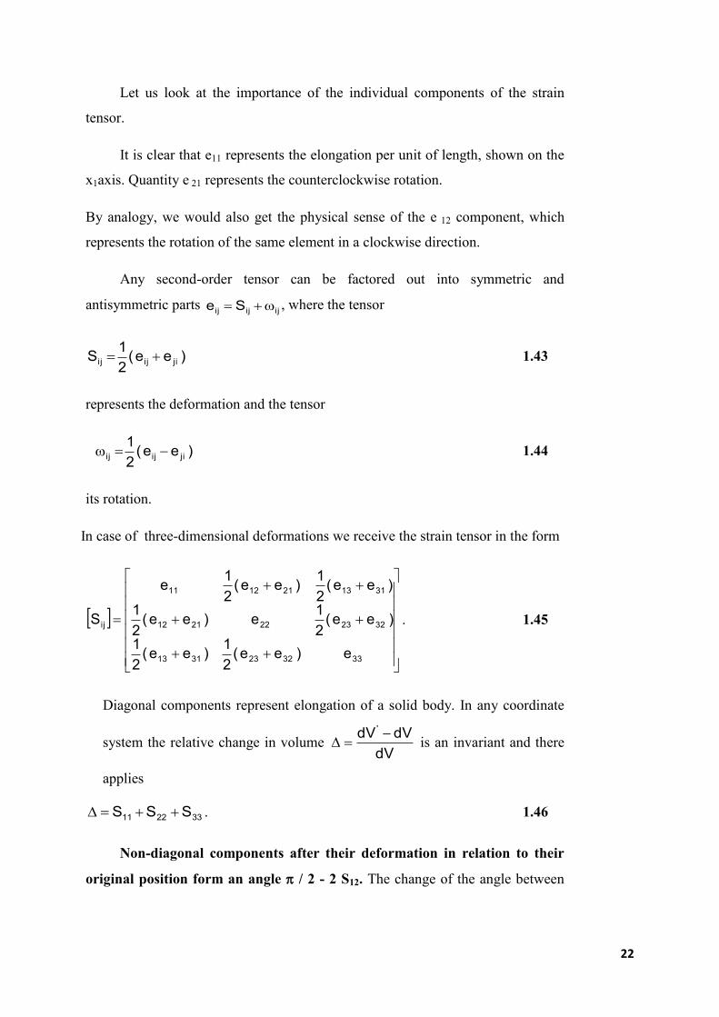
In case of three-dimensional deformations we receive the strain tensor in the form

3332233113

3223222112

3113211211

ij

e)ee(2

1)ee(

2

1

)ee(2

1e)ee(

2

1

)ee(2

1)ee(

2

1e

S . 1.45

Diagonal components represent elongation of a solid body. In any coordinate

system the relative change in volume dV

dVdV ' is an invariant and there

applies

332211 SSS . 1.46

Non-diagonal components after their deformation in relation to their

original position form an angle / 2 - 2 S12. The change of the angle between

23

the two mutually perpendicular sections dxi, dxj is due to shear strain Sij, and thus

equal to -2S ij .

So far we have dealt with changes of the samples length due to physical

stresses. Changes of the samples length, however, can also have different causes,

and this can be e.g. thermal expansion.

For small temperature changes we can consider the deformation to be

homogeneous, and for the strain tensor we can write

TS ijij . 1.47

ij are called coefficients of expansion. Let us note that both [ ij ] and [ Sij ]

are second-order tensors.

1.5. Elastic constants tensor

In these course tasks we will expect these distortions to be small (flexible)

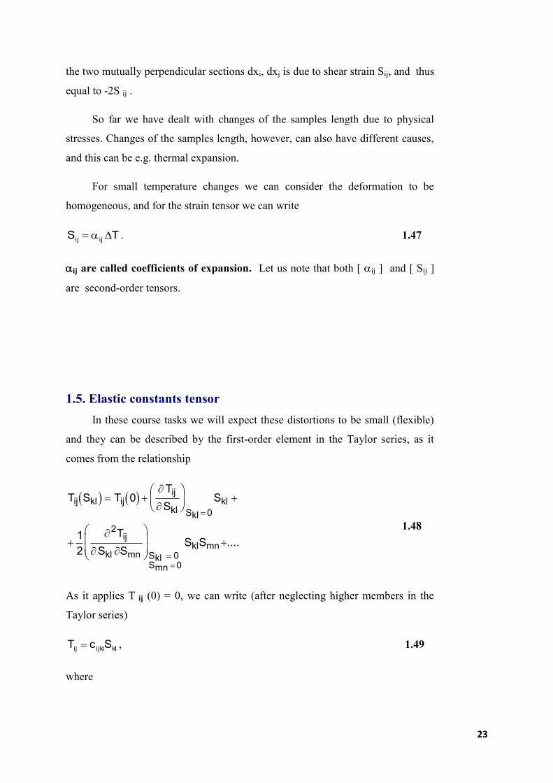
and they can be described by the first-order element in the Taylor series, as it

comes from the relationship

T S TT

SS

T

S SS S

ij kl ijij

kl Skl

kl

ij

kl mn SklSmn

kl mn

0

1

2

0

2

00

....

1.48

As it applies T ij (0) = 0, we can write (after neglecting higher members in the

Taylor series)

klijklij ScT , 1.49

where

24

cT

Sijkl

ij

kl Skl

0

. 1.50

Expression 1.50 is a modulus of elasticity tensor and the expression 1.49

we call the generalized Hook´s law . The tensor of elastic constants is the fourth-

order tensor and it has 3 4 =

81 components. Stress and strain tensors are

symmetrical, and therefore the values of elastic constants do not change when

switching the first two or the other two indexes, and so it is

c c c cijkl jikl ijkl ijlk ; . 1.51

Relationship 1.51 reduces the number of independent elastic constants to 36.

Further reduction, as we shall see later, will be caused by the symmetry of

crystals.

In respect to the above stated fact that the order of indices (e.g. i, j ) is

commutable, there are only six pairs of combinations, numbered from one to six,

as follows:

(11) 1, (22) 2, (33) 3, (23) = (32) 4, (31) = (13) 5, (12) = (21) 6.

1.52

With the unevenly pairs of indices the "renumbering" can be determined in a way

that we add figure 3 to the missing number of the triple group 1,2,3.

If we would like to express distortion as a stress function, then the

generalized Hook´s law has the form

,TsS klijklij 1.53

where the set of values sijkl, the so-called coefficients of compliance, is again the

fourth-order tensor. For the mathematical expression of the elastic constants

tensor [cijkl] and the compliance tensor [sijkl] in the form of matrix it applies that

s= (c)-1

or s c = , where is the Kronecker symbol, which we can

also interpret as a matrix, in which the both tensors s, c are mutually inverse.

25

Note.

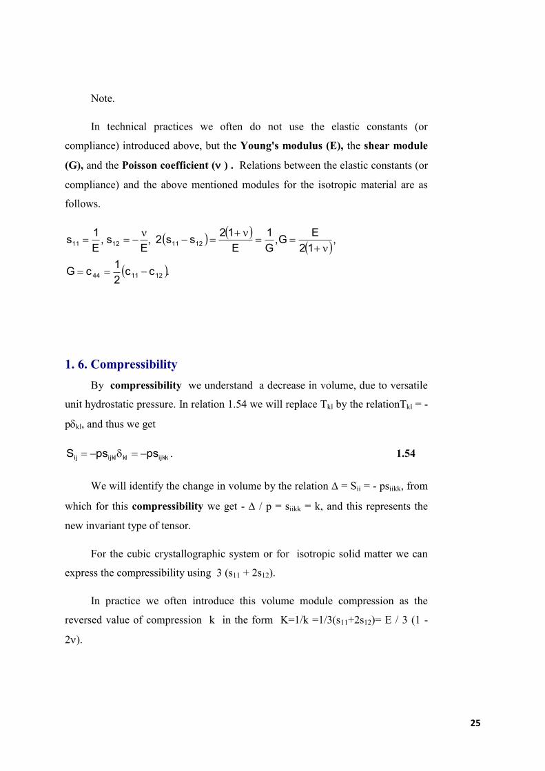
In technical practices we often do not use the elastic constants (or

compliance) introduced above, but the Young's modulus (E), the shear module

(G), and the Poisson coefficient ( ) . Relations between the elastic constants (or

compliance) and the above mentioned modules for the isotropic material are as

follows.

.cc2

1cG

,12

EG,

G

1

E

12ss2,

Es,

E

1s

121144

12111211

1. 6. Compressibility

By compressibility we understand a decrease in volume, due to versatile

unit hydrostatic pressure. In relation 1.54 we will replace Tkl by the relationTkl = -

pkl, and thus we get

ijkkklijklij pspsS . 1.54

We will identify the change in volume by the relation = Sii = - psiikk, from

which for this compressibility we get - / p = siikk = k, and this represents the

new invariant type of tensor.

For the cubic crystallographic system or for isotropic solid matter we can

express the compressibility using 3 (s11 + 2s12).

In practice we often introduce this volume module compression as the

reversed value of compression k in the form K=1/k =1/3(s11+2s12)= E / 3 (1 -

2).

26

1. 7. Impact of lattice symmetry on tensor representation

The periodicity of lattice reduces the number of possible elements of

symmetry and creates relationships between some of them, and so there are only

seven groups of symmetries, each of which determines one crystallographic

system.

There are two basic types of elementary symmetric operations. It is a direct

and inverse symmetry.

Elementary direct symmetries are related to the axis of symmetry, with the axis

of symmetry An of the n order, where n is a whole number if by rotating the

crystal around this axis by angle 2 / n this crystal gets into the starting position,

in which it was before rotating.

Inverse symmetry is bound to the centre of symmetry and the inverse axis.

The centre of symmetry C corresponds to an inverse transformation of the

crystal with respect to a point.

The inverse axis of the n order, denoted as An

i re-transforms the crystal

from the initial position by turning it using the 2 / n angle and the subsequent

inversion with regard to the point. Thus the equation An

i = AnC = C An

applies.

The plane of symmetry is a special case of inversion axis of the second

order, or the mirror plane M perpendicular to the axis at the point of inversion,

and thus A 2

i = M.

Equally, the centre of symmetry is equivalent to the inverse axis of the first

order, and so it is C = A1i .

As we have already mentioned above, the periodicity of the crystal structure,

except for reducing the types of symmetry, also leads to the relationships of

equivalence between the individual symmetries .

As a result of crystals symmetry only certain types of symmetrical

operations may exist and only the axis of a certain order symmetry. Overall,

27

there are thirty-two classes of crystals point symmetry. For the three

dimensional lattice there are fourteen types of so-called Bravaiselementary

lattice types. These fourteen types of lattices are grouped in seven

crystallographic systems, according to the seven types of elementary cells.

Principles applicable to the so-called point symmetry of the crystal lattices can be

summed up into the following statements.

1. Each straight line parallel to the axis of symmetry of the n order, which

passes through a node of lattice, is the axis of symmetry of the same order.

2. Each axis of symmetry passing through the node is identical with the

lattice order.

3. Each node of the lattice is the centre of symmetry.

4. The axis of symmetry of the order n 2 creates n of the perpendicular

axes of the second order.

In the next section we will focus on symmetrical operations, which are

permitted in respect to the lattice periodicity, and which determine the seven

crystallographic systems.

For greater clarity there are the individual symmetrical operations and geometric

parameters of the individual crystallographic systems stated in Figure 1.8 .

At the very beginning of our chapter on the impact of symmetry on the

tensor representation of physical quantities, we will deal with second-order

symmetrical tensors, which describe physical properties which have central

symmetry. These tensors have six independent components, if they relate to any

coordinate system.

If, however, the crystal has a certain symmetry, the number of independent

components is declining. The symmetry of the characteristic area of the tensor is

identical to the symmetry of the given physical property described by the tensor.

In the context of physical properties symmetry, and the point symmetry of

the crystal it is useful to come closer to the so-called Neuman´s principle that

says:

28

Elements of physical quantity symmetry, which characterises the

crystal, involve elements of point group crystal symmetry.

Physical quantity may therefore have a certain symmetry, which is manifested

independently of the symmetry in a given crystal. In accordance with Neuman´s

principle, however, the physical property must also have all the elementary

symmetries, which have a crystal. For example, the flexibility of a hexagonal

crystal is not only centrally symmetrical, but also has elements of symmetry of

this crystalline system.

If we introduce transformation matrix l , we get

...pqr..

'

..ijk.. SS ......... r

k

q

j

p

i lll , 1.55

Therefore, the invariance of the physical properties in relation to

selected symmetrical operations leads to the transformation equation

...pqr.....ijk.. SS ......... krjqip lll 1.56

Let us go, however, to some specific cases. The centre of symmetry is described

using matrix 1.15 or in a short entry ij

j

i , whereij is the Kronecker symbol.

Then ...ijk.....ijk.. SS ......... kkjjii lll ,

or for the tensor of n order it is valid S S...ijk..

n

...ijk.. 1

If n is odd, then (- 1) n =

-1, and therefore all tensor components are zero.

This result can also be interpreted, so that centrally symmetrical crystals cannot

have physical properties described by the tensors of unpaired orders. This applies,

for example, to piezoelectric and pyroelectric phenomenon, which are described

precisely by tensors of the third order. If n is paired, there are no changes caused

by the centre of symmetry.

At the very beginning of our chapter on the impact of symmetry on the

tensor representation of physical quantities, we will deal with second-order

symmetrical tensors, which describe physical properties which have a central

29

symmetry. These tensors have six independent components, if they relate to any

coordinate system.

If, however, the crystal has a certain symmetry, the number of independent

components is declining. The symmetry of the characteristic area of a tensor is

identical to the symmetry of the given physical property described by the tensor.

In the context of physical properties symmetry, and the point symmetry of

the crystal it is useful to come closer to the so-called Neuman´s principle that

says:

Elements of physical quantity symmetry, which characterises the

crystal, involve elements of point group crystal symmetry.

The physical quantity may therefore have a certain symmetry, which is

manifested independently of the symmetry in a given crystal. In accordance with

Neuman´s principle, however, the physical property must also have all the

elementary symmetries, which have a crystal. For example, the flexibility of a

hexagonal crystal is not only centrally symmetrical, but also has the elements of

symmetry of this crystalline system.

If we introduce transformation matrix l, we get

...pqr..

'

..ijk.. SS ......... r

k

q

j

p

i lll , 1.57

Therefore, the invariance of the physical properties in relation to selected

symmetrical operations leads to the transformation equation

...pqr.....ijk.. SS ......... krjqip lll 1.58

Let us go, however, to some specific cases. The centre of symmetry is described

by the relationship ij

j

i , where ij is the Kronecker symbol. Then, or more

precisely for the tensor of the n order there is valid S S...ijk..

n

...ijk.. 1

If n is odd, then (- 1) n =

-1, and therefore all tensor components are zero.

This result can also be interpreted, so that centrally symmetrical crystals

cannot have physical properties described by tensors of unpaired orders.

This applies, for example, to piezoelectric and pyroelectric phenomenon, which

30

are described precisely by tensors of the third order. If n is paired, there are no

changes caused by the centre of symmetry. Relevant symmetrical operations in

crystalographic systems is presented in Figure 1.8.

Figure 1.8. Crystallographic systems and their relevant symmetrical operations

Summary of terms

Transformation of coordinates and tensors, properties of the second-order tensors,

stress tensors, distortions and Hook´s law in general form, compressibility, the impact of

lattice symmetry on the the number of independent components of the tensor.

Questions to the topic

1. How to transform the second-order tensor?

2. What relationship determines the stress tensor constituents?

3. Explain Hook´s law in its general form.

4. How can we calculate the compressibility of anisotropic material?

31

5. What is the impact of symmetry on the number of independent components of the second-

order tensor?

6. Explain the term invariant tensor, and what it determines?

32

2. The basics of statistical physics and quantum mechanics

Study time 5 hours

Objectives

you will be familiar with the statistical description of large groups of

particles.

you will get acquainted with the basics of the wave description of

particles.

you will understand the difference between the micro and macro world.

you will understand the importance of introducing the concept of phase

space.

LLecture

2.2 1. Statistical interpretation of a physical systems description with

many particles

In this section we will formulate the basic relations of a multi-

particle system description and monitor their progress, depending on the

changes of various physical parameters. Why is there a need for the

introduction of another mathematical approach, as we were used to

traditional Newton´s physics? The answer to this question is presented

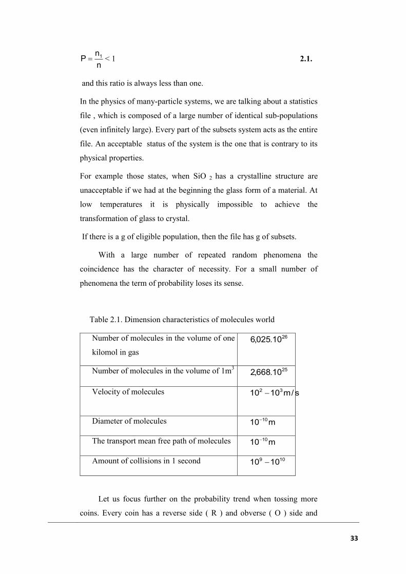
in Table 2.1.

From the numbers above we can see that the multi-particle systems

descriptions, such as e.g. gases, using the differential equations of

Newton´s mechanics, would be extremely difficult, but in particular

scientifically difficult to solve.

Therefore, for the description of multi-particle systems the methods of

mathematical statistics are used. Mathematical probability is defined as

the ratio of expected phenomena to all 1n possible phenomena n ,

which can be expressed by the relation

33

n

nP 1 < 1 2.1.

and this ratio is always less than one.

In the physics of many-particle systems, we are talking about a statistics

file , which is composed of a large number of identical sub-populations

(even infinitely large). Every part of the subsets system acts as the entire

file. An acceptable status of the system is the one that is contrary to its

physical properties.

For example those states, when SiO 2 has a crystalline structure are

unacceptable if we had at the beginning the glass form of a material. At

low temperatures it is physically impossible to achieve the

transformation of glass to crystal.

If there is a g of eligible population, then the file has g of subsets.

With a large number of repeated random phenomena the

coincidence has the character of necessity. For a small number of

phenomena the term of probability loses its sense.

Table 2.1. Dimension characteristics of molecules world

Number of molecules in the volume of one

kilomol in gas

2610.025,6

Number of molecules in the volume of 1m3 2510.668,2

Velocity of molecules s/m1010 32

Diameter of molecules m10 10

The transport mean free path of molecules m10 10

Amount of collisions in 1 second 109 1010

Let us focus further on the probability trend when tossing more

coins. Every coin has a reverse side ( R ) and obverse ( O ) side and

34

when tossing a set of coins the different ratio of R:O appears. To

describe such a process we use combinatorics. If every coin is an

individual element of the coins file, and we number them from 1 to 10,

and we take into consideration only one side of them, we can build out

of these ten numbered coins a total of 3,628,800 arranged series of

different sequences of numbered coins, as

36288001......8.9.10!10!n .

After each toss of these coins we get the different ratio of R and O in

the series, but with the identical ratio and in various combinations. If we

consider variations of both sides of the coins in the series with ten coins

( R= 0-10, L=10 - 0), according to the rules of combinatorics, the

number of all variations is 1024210 .

For example, for four coins we receive 1624 variations. Hence, we

can make 16 patterns with four coins, in which there are different

variations in sides R,O. The probability of phenomenon, in which when

tossing ten coins we will get all R or only O is 10

10

22

1

, and for

that case we need to toss them at least 1,024 times.

For a number of equal and repeating cases the following relationship

applies

!nn!n

!nn

!n!n

!n

11

21

21

, 2.2.

where 21 nnn is the number of expected phenomena.

For 21 nn we get relationship

!n!n

!ng

11

, 2.3.

which was called by Planck thermodynamic probability, and it is also

called the statistical weight, or the degree of system degeneration ( the

number of equal conditions) .

Probability that we will toss Ln1 and Rn2 will be given by the

35

relation

nn

21

2

!L!R

!LR

2

!n!n

!n

P

, where

21

n

21 nnn,10242,Ln,Rn .

Let us now further investigate the interpretation of thermodynamic

probability. Imagine the two identifiable (marked, but identical)

molecules in an enclosed space with a filter, which divides the space

into two halves. Possible distribution of molecules in each part (

statistical conditions or also microstates ) is in the Table 2.2.

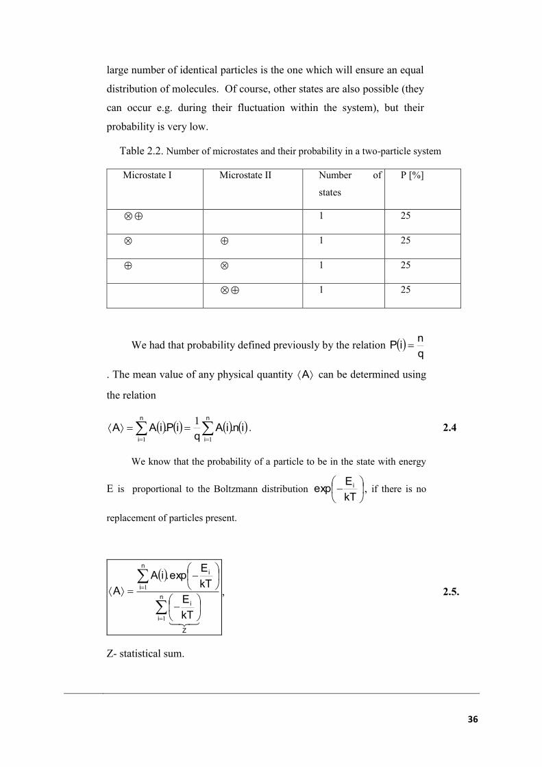
If we apply this example of the above mentioned relations, we will

get the total number of microstates of 422 , but only three

thermodynamic (also called macrostates) states, or the state of gas

determined by the group of molecules, regardless of which individual

molecule creates this state of gas. Equal distribution of molecules on

both sides of the filter appears twice ( 2!1!1

!2

!n!n

!ng

11

) and the

total probability P of this state is thus 50 percent.

Lets´ investigate the further development of such a twin-

microstate system with an increasing number of molecules. For four

molecules we get 1624 states, while the even distribution will

appear in six cases, or 6!2!2

!4

!n!n

!ng

11

.

The probability of the spontaneous compression of molecules in one

part of this system decreases with an increasing number of molecules. If

it was 25 percent for two molecules, in case of four molecules it will be

only 6.25 percent, and with ten molecules the figure will be 410.8

percent.

What is more interesting, the thermodynamic probability g of the

state of equilibrium (distribution), on the other hand, will grow quickly.

With ten molecules these states reach 252, with 100 molecules it is even

2810.15,11 , and with a thousand molecules we get 29910.7,2 . Based on

these considerations it is clear that the most probable distribution of a

36

large number of identical particles is the one which will ensure an equal

distribution of molecules. Of course, other states are also possible (they

can occur e.g. during their fluctuation within the system), but their

probability is very low.

Table 2.2. Number of microstates and their probability in a two-particle system

Microstate I Microstate II Number of

states

P [%]

1 25

1 25

1 25

1 25

We had that probability defined previously by the relation q

niP

. The mean value of any physical quantity A can be determined using

the relation

in.iAq

iP.iAAn

i

n

i

11

1. 2.4

We know that the probability of a particle to be in the state with energy

E is proportional to the Boltzmann distribution

kT

Eexp i , if there is no

replacement of particles present.

n

i

Z

i

n

i

i

kT

E

kT

Eexp.iA

A

1

1

, 2.5.

Z- statistical sum.

37

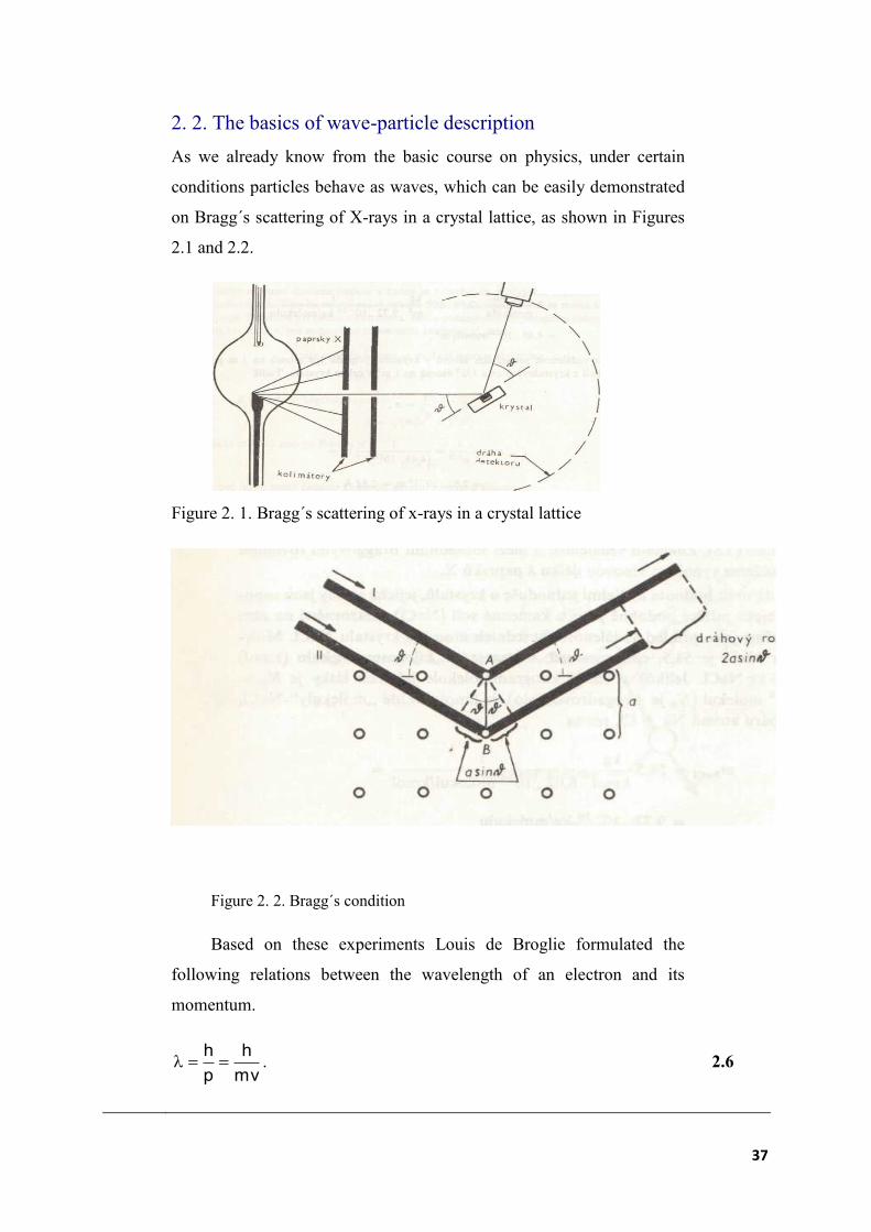
2. 2. The basics of wave-particle description

As we already know from the basic course on physics, under certain

conditions particles behave as waves, which can be easily demonstrated

on Bragg´s scattering of X-rays in a crystal lattice, as shown in Figures

2.1 and 2.2.

Figure 2. 1. Bragg´s scattering of x-rays in a crystal lattice

Figure 2. 2. Bragg´s condition

Based on these experiments Louis de Broglie formulated the

following relations between the wavelength of an electron and its

momentum.

mv

h

p

h . 2.6

38

Wave functions themselves does not provide any relevant physical

information, as it is comprehensive.

Physical signification, however, has the product of real and imaginary

components 22222* B+A=Bi-A=ψψ , the so-called probability

density , which represents a real number. This product gives the probability

that a particle will occur at a given time and at a given space.

On the basis of such a wave function interpretation then W.

Heisenberg formulated the so-called uncertainties relation, which does

not to simultaneously allow the same accuracy to measure a coordinate

and momentum because of the principle.

ΔxΔp≥h/ 2π. 2.7

Let us now describe the n particles system using the wave

functions. Such a "total" wave function can be expressed as a product of

functions of the individual parts in the form

( ) ( ) ( ) ( ).nψ.......2ψ1ψ=N:::::.2.1ψ 2.8

If there is one particle in state a and the second in state b, the probability

density should not change and there must apply

( ) ( )22

1,2ψ=2,1ψ. 2.9

Wave functions ( )1,2ψ after replacement of particles may be either

symmetrical, or antisymmetric, and so one of the two following relations

applies

( ) ( )1,2ψ=2,1ψ ,

( ) ( )1,2ψ=2,1ψ- . 2.10

If there is particle 1 in state a and particle 2 in state b, or particle 1 in

state b and particle 2 in state a, this equation can be applied

( ) ( )

( ) ( ).1ψ2ψ=ψ

,2ψ1ψ=ψ

ba2

ba1

2.11

39

Both functions properly describe the system, and so the resulting

function of the whole system is given by their linear combination

( ) ( ) ( ) ( )( )1ψ2ψ+2ψ1ψ2

1=ψ babas

,

( ) ( ) ( ) ( )( )1ψ2ψ-2ψ1ψ2

1=ψ babaa

. 2.12

Antisymmetric features describe those particles with a half-integer

spin, so-called Fermions ( electrons, protons, neutrons..)

Particles with an integer spin, such as photons, are described using

symmetrical functions, and they are also referred to as Bosons,

2. 3. Quantum statistics

As we already know from the previous parts of this textbook,

which was dealing with the quantum-mechanical principles of the micro

world, an electron can be in only one energy state at the same time,

with two different orientations of spins (the Pauli principle). Particles

operating under this principle are also called fermions (and include, e.g.

also 3 He - 2 protons, 1 neutron). Let us return to the model used in

Chapter 4, and we will assume that the system (with only one electron

possessing energy , or a free-vacant, and its energy is equal to zero) is

in the thermal and diffusion contact with a reservoir, as seen in Figure

2.3.

Figure 2. 3. Possible states of a fermion according to the Pauli

1. R

e

s

e

r

v

o

i

r

vacant

energy

=0

2. R

e

s

e

r

v

o

i

r

1

electro

n

energy

40

principle

Large amount 9 (not only there is an exchange of energy taking

place within the system, but also an exchange of particles), we can write

for fermions the following

Z = 1 + exp(-/), 2.13

because kTkTkTkT

0

e1eeeZ

. For the mean value of the

system occupancy we get the expression

kT

kT

e.1

e.n

, 2.14.

or we define the function

( )

1+e

1=εn=)ε(f

kT

με

, 2.15

which we call Fermi - Dirac distribution.

In the subject of solid physics the chemical potential at absolute

zero is called Fermi energy or even the Fermi level.

If at any temperature the value the energy of a system is equal to the

chemical potential, then the medium-sized occupancy of the system is

equal to one-half, which is based on the relationship

.5,011

1

1kT/exp

1f

Development of the Fermi-

Dirac partition function is shown in Figure 2. 4.

41

0 0,2 0,4 0,6 0,8 1,0 1,2 1,4

0,2

1,0

0,8

0,6

0,4

1f( )=

Figure 2. 4. Fermi-Dirac distribution 5,0 μττ

Note:

It should be noted that the occupation of the levels in the Fermi-

Dirac partition function is identical to the probability of its

occupancy.

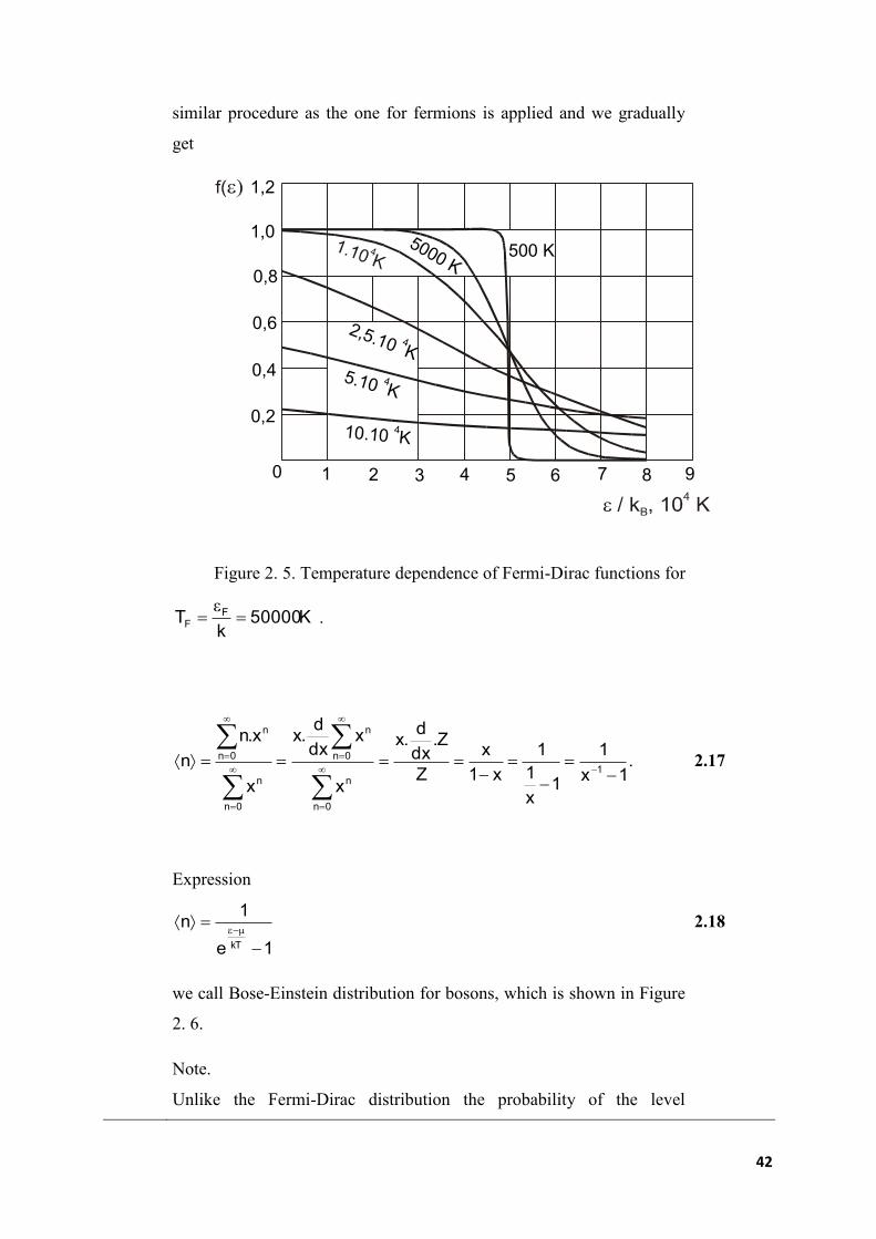
Temperature dependence of the Fermi-Dirac function for

K50000k

T FF

ε is shown in Figure 2. 5.

In addition to fermions there is also another class of particles with

an integer spin (e.g. photons, 4 He, 2 protons, 2 neutrons), which are

subject to other statistical rules as fermions. To these particles the Pauli

principle does not apply, and so the system, which is in thermal and

diffusion contact with the reservoir can be filled with any number of

particles, and for a large amount this expression is valid

x1

1=x=e=

kT

εnμnexp=)kT,μ(Z

0=n

n

0=n

n

kT

εμ

0=n

∑∑∑∞∞∞

, 2.16.

where x = exp((-)/kT). The sum of geometric series for x 1 converts

a for x 1 diverges. For the mean number of particles in the system a

42

similar procedure as the one for fermions is applied and we gradually

get

987654321

0,8

0,6

0,4

0,2

1,0

1,2

0

500 K5000 K

2,5.10 4K

5.10 4K

10.10 4K

Figure 2. 5. Temperature dependence of Fermi-Dirac functions for

K50000k

T FF

ε .

.1x

1

1x

1

1

x1

x

Z

Z.dx

d.x

x

xdx

d.x

x

x.n

n1

0n

n

0n

n

0n

n

0n

n

2.17

Expression

1e

1n

kT

2.18

we call Bose-Einstein distribution for bosons, which is shown in Figure

2. 6.

Note.

Unlike the Fermi-Dirac distribution the probability of the level

43

occupancy is not in the bosons statistics identical to its occupancy, as it

was in the case with fermions. The less the energy, the greater the

number of particles.

210-1-20

Boseho -Einsteinoverozdelenie

Fermiho -Diracoverozdelenie

n (

1

2

3

4

Figure 2. 6. Bose-Einstein and Fermi-Dirac distribution.

In Figure 2.6 you can also see that for the 'great power' both

distributions valid for the world of quanta within limits are getting

near each other (the unit for the denominator ceases to play an

important role) and pass into the "traditional" Maxwell-Boltzmann

distribution in (if we contemplate the pre-exponential member).

.

2. 4. Schrödinger equation

Let's write an equation for a wave travelling in the direction of the axis x in

the form

Ψ=Aexp[-iω(t-x/v)]. 2.19

As it applies

E=hν

and 2.20

λ=h/p

44

we can rewrite the equation 2.19 as

Ψ=Aexp[-i/ħ(Et-xp)], 2.21

which is valid for a free particle .

In order to monitor the dynamics of phenomena, which means

changes in coordinates, or time, we have to calculate the relevant

derivations.

2

2

2

2 Ψp-=

x∂

Ψ∂

2.22.

ΨiE-=

t∂

Ψ∂

For the total energy of particles the following relation applies

V+m2

p=E

2

, 2.23

or after adjustment

ΨV+m2

Ψp=ΨE

2

. 2.24

Further applies

t

Ψ

i-=ΨEΨ

iE-=

t

Ψ

∂

∂→

∂

∂

2.25

Ψp=x

Ψ- 2

2

2

2

∂

∂

where we come to the time-dependent form of Schrödinger equation of

0=ΨEm2

+x

Ψ→ΨV-

x

Ψ

m2=

t

Ψ

i 22

2

2

22

∂

∂

∂

∂

∂

∂, 2.26

45

2. 5. The phase space

In traditional mechanics, the immediate status of a particle is

clearly described by the value of coordinates and pulse, which, as we

know, are in principle also measurable with the same accuracy. The laws

of Newton´s mechanics with regard to their deterministic nature enable

us to identify the behaviour of particles at the time. Entering

instantaneous values of generalized coordinates q and generalized pulse

p is equivalent to the point within the two-dimensional space p vs. q,

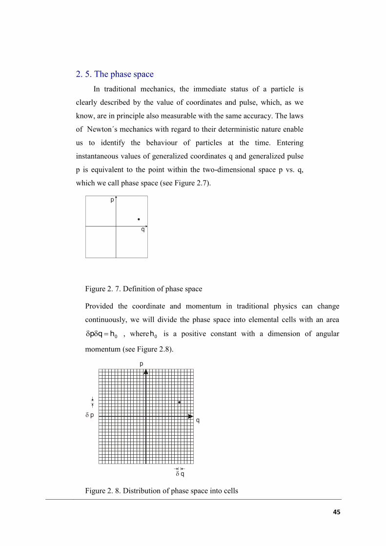
which we call phase space (see Figure 2.7).

Figure 2. 7. Definition of phase space

Provided the coordinate and momentum in traditional physics can change

continuously, we will divide the phase space into elemental cells with an area

0hqp , where 0h is a positive constant with a dimension of angular

momentum (see Figure 2.8).

Figure 2. 8. Distribution of phase space into cells

46

In order for the status particles to be described it is sufficient to

prove that the coordinate is in the range of phase space qq,q and

the momentum is from the interval pp,p . Now, we need to answer

the question what size must constant 0h be? In traditional physics its

value may be infinitely small, and our task is reduced to answer the

question, what is the "serial " number of a cell in the phase space, in

which the coordinate and momentum of a particle are situated?

As we know from quantum mechanics, the volume of a phase

space cell is clearly determined by the Heisenberg uncertainty principle.

In conclusion here are practical technical applications of the phase

space.

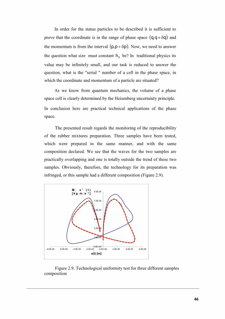
The presented result regards the monitoring of the reproducibility

of the rubber mixtures preparation. Three samples have been tested,

which were prepared in the same manner, and with the same

composition declared. We see that the waves for the two samples are

practically overlapping and one is totally outside the trend of these two

samples. Obviously, therefore, the technology for its preparation was

infringed, or this sample had a different composition (Figure 2.9).

Figure 2.9. Technological uniformity test for three different samples

composition

0.0E+00

1.5E-05

3.0E-05

4.5E-05

6.0E-05

7.5E-05

9.0E-05

-8.0E-05 -6.0E-05 -4.0E-05 -2.0E-05 0.0E+00 2.0E-05 4.0E-05 6.0E-05

M . x ' ( t ) [ k g . m . s - 1 ]

x(t) [m]

47

Summary of terms

Statistical description multi-particle systems, mean values of physical quantities, wave particle

description, probability density, Fermi-Dirac distribution function, Bose-Einstein distribution

function, Schrödinger equation, the phase space.

Questions to the topic

1. How is the probability of a phenomenon defined?

2.What is the thermodynamic probability?

3. How do we calculate the mean value of a physical quantity?

4. Characterize Fermi-Dirac statistics.

5. Characterize Bose-Einstein statistics.

6. Explain the Schrödinger equation.

7.What are symmetrical and antisymmetric wave functions?

8. Explain the term the wave function of particles.

9. When can the electron be seen as a traditional particle?

10. Explain the Heisenberg uncertainty principle.

11. Explain the concept of the phase space.

48

3. Viscous and viscous-elastic behaviour of materials

Time for learning: 5 hours

you will be familiar with viscous and viscous-elastic concepts.

you will learn about these environments models.

you will get acquainted with the characteristics of real materials.

you will learn to understand microstructural aspects of materials flow.

you will understand the processes accompanying material flow.

Lecture

3. 1. Characteristics of viscous and viscous-elastic environments

The term viscosity is most frequently associated with liquid and gaseous

states. Viscosity is a physical phenomenon caused by Van der Waals´ forces

acting among particles in liquid or gas during their motions. If this movement is

only of a "shear" nature, then, as we already know from the basic course on

physics, Newton´s viscous law applies as

dy

dvTyx , 3.1.

where T is stress and η is the dynamic viscosity . We call them Newton´s fluids.

Real fluids, however, are different from Newton´s ones. Also water, as a liquid

with a relatively low viscosity, responds "flexibly", if we apply to it e.g. enormous

stresses in short pulses. This phenomenon is well known e.g from "spoiled

jumps" into water, when we hit our abdomen (the flexible response of water is

felt sufficiently in that very moment). Development over time of a mechanically

loaded viscous environment thus also depends on the duration of load action.

We know from our experience that on asphalt roads so-called "tracks"

appear, caused by heavy lorries and vehicles, especially during the summer time.

49

Certainly, you can recall the prints of female high-heel shoes, the so-called

needles, in asphalt during the summer months. We also know that if we heat

honey, it becomes more liquid, and we can find even more similar examples.

There is, however, one fact, namely that material viscosity is, along with the

length of exposure and the size of attached mechanical tension (a so-called

thixotropic substance) also a function of temperature.

In our interpretation of this phenomenon we will draw on the so-called the

hole model of fluids. In this model, it is assumed that fluid is composed of

molecules and of vacant places, so-called holes, which may appear in a liquid, e.g.

after the evaporation of some molecules. The jump of a molecule into a new, more

energy-advantageous position is only possible if the neighbouring place is free,

and thus there is a hole. The concentration of such holes (the ratio of vacant places

n to the total sum of the nodes N of this structural network) will be

RT/HeN

n , 3.2.

Where ΔH is enthalpy, which is needed to create a hole (and it is approximately

equal to 2/5.ΔH cal. ), R is the gas constant and T is the absolute temperature.

Molecules oscillate around equilibria positions, and 2ν-times per second attack the

surrounding potential barriers. Then for the frequency of possible jumps of

molecules we get

BA

RT/QRT/H HHQ;e2eN

n2

1

. 3.3

The first of enthalpies represents the activation enthalpy, necessary for the

creation of holes, and the second represents the height of barriers, which the

molecule must overcome in self-diffusion. If we identify the coordination

number of the z molecule (the number of nearest neighbours is z), then for the

frequency of jumps it is zτ

1=ν .

If the diffusion process is assisted by the external force F, then the

molecules will be moving in the direction of this force and the mean speed of

50

molecules will be proportional to this force, the coefficient of proportion is called

the mobility of molecules.

Fqv . 3.4

If between the liquid layers, which are mutually slipping, the distance δ is equal

to the atomic distance, then the following relationship applies

δq

1=η 3.5

and for dynamic viscosity coefficient we get (without stating further steps, which

are of a mathematical character)

RT/Q

33e

νδ2

zkT=

δ

τzkT=η , 3.6

where k is the Boltzmann constant. We can see that the dynamic viscosity

coefficient decreases with increasing temperature, as we have discussed

above. The mentioned model is of course a qualitative one, and for different types

of materials and temperature ranges of other relations are also used.

Now we extend our knowledge of the physical interpretation of viscous flow

to polymers and rubbers. It is well known that molecular "jumping over" takes

place mainly in amorphous areas, while for crystallite they occur in their

interfaces or degraded areas. It may also result in a partial turn of all crystallites.

The kinetics of flow is described using two different processes.

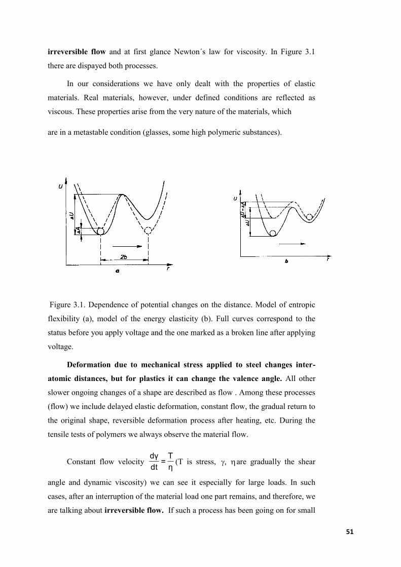
Let us analyse the first process. Molecules jumping over in the direction of

flow lead to an arrangement with less entropy without changing their internal

energy; this process is called entropic elasticity. The process is shown in Figure

3.1a. It can also cause filling states with higher energy, which is conditioned by

the existence of nodal points, and this is so-called energy flexibility, and it

corresponds to the situation displayed in Figure 3.1b.

In the later case, molecules or their parts distract from their surroundings

and the nodal points shall cease to exist. The distribution of this potential energy

does not change on average, as there are new potential barriers being built, which

have the same energy distribution as the original one. This flow is called

51

irreversible flow and at first glance Newton´s law for viscosity. In Figure 3.1

there are dispayed both processes.

In our considerations we have only dealt with the properties of elastic

materials. Real materials, however, under defined conditions are reflected as

viscous. These properties arise from the very nature of the materials, which

are in a metastable condition (glasses, some high polymeric substances).

Figure 3.1. Dependence of potential changes on the distance. Model of entropic

flexibility (a), model of the energy elasticity (b). Full curves correspond to the

status before you apply voltage and the one marked as a broken line after applying

voltage.

Deformation due to mechanical stress applied to steel changes inter-

atomic distances, but for plastics it can change the valence angle. All other

slower ongoing changes of a shape are described as flow . Among these processes

(flow) we include delayed elastic deformation, constant flow, the gradual return to

the original shape, reversible deformation process after heating, etc. During the

tensile tests of polymers we always observe the material flow.

Constant flow velocity η

T=

dt

γd(T is stress, , are gradually the shear

angle and dynamic viscosity) we can see it especially for large loads. In such

cases, after an interruption of the material load one part remains, and therefore, we

are talking about irreversible flow. If such a process has been going on for small

52

stresses, we can say that this material does not have supple strength. Supple

strength was first seen in crystals, and this deformation is usually called plastic.

For illustration in Figure 3.2 there is shown the rate of change for the original

right angle γ of the prism, on which tangential stress is applied, as a function of

the attached mechanical stress for various types of materials.

Deformation of vulcanised natural rubber is almost immediate, and it is

permanent only for a tiny part of this material. After that load interruption

material returns to its original state and hysteresis is small (the hysteretic curve

has a small area), as we can see in Figure 3.3.

The measured elastic deformation of rubber is composed of two parts. This

deformation leads both to a reduction in entropy due to the increase in the

orderliness of this system, and this process will also be reflected in a fall of

specific heat capacity of this material. Module E 1 flowing from this decrease in

entropy is directly proportional to its absolute temperature. In non-ideal

vulcanized rubber one part of deformation work is bound to internal energy,

resulting in a change of inter-atomic distances, but in particular the changes of

valence angles and the corresponding change of module E 0 . For the overall

module then we get10 E

1

E

1

E

1 , or

T

tatankonš

E

1

E

1

0

.

3. 2. Newton´s fluid (a), non-Newton fluid (b), substance with supple

strength (c)

53

3.3. Hysteretic curve. Mechanical stress versus deformation

As can be seen from Figure 3.4 with increasing temperature the module

increases (curve a), which is the result of the entropic nature of the flexibility

rubber, but for plastics it decreases (curve b), as the share of contributions of

reversible, and time-dependent deformation increases.

Change of the module between points A and B depends on the transition to

the ideal flexible behaviour of the material under the glass transition temperature.

Rubber substance (a), viscous elastic substances (b).

Figure 3. 4. Dependence of module E on temperature.

The module of rubber is significantly lower than those of the other

substances. The Elastic deformation of rubber in many cases exceeds the initial

54

length of material. It is therefore not possible in one diagram to display the stress

and deformation of rubber, plastic and steel.

Such a comparison is only possible using a logarithmic scale, as seen in

Figure 3. 5.

Let us now describe polymers in terms of their structures and physical

properties. As with all substances, also for polymers we can define three basic

states: gas, liquid and solid. Despite the general similarities, in polymers there are

certain specifics properties, which distinguish them from low molecular

substances.

.

3. 5. Tensile waves in a logarithmic scale for rubber (a), viscous elastic

substance (b), steel (c)

In general the gaseous state is characterised by an intensive flow of particles,

where the distances between molecules are great. As the interaction of particles,

within the meaning of attractive force, decreases with the sixth square distance,

for molecules in gaseous state the mutual attractive forces in view of the distance

between molecules can be practically disregarded.

55

In the liquid state the thermal movement of molecules is still very intense, but in

contrast to the gas state, the distances between molecules are considerably smaller

and the molecules strongly affect each other.

In the solid state, the intensity of heat movement is reduced so much that it

is not sufficient to break up the molecular contacts. Molecules will take a

permanent, defined position within the space, and only perform vibratory

movements with a frequency of 10 13-14

Hz . The distances between molecules do

not differ too much from the liquid state, which can be easily proven by

comparing the density of substances in all three states. While the difference in

density between gas and liquid reaches several orders, the difference between the

density of liquid and solid substances is small. It can be said that the distance

between the particles are approximately on the same level of molecular sizes.

From differences in molecules mobility also some significant differences in

properties result.

For the liquid state the intensive translational movement of molecules along

with rotary and vibration movement is typical, in the solid state all molecules are

occupying more or less constant positions, and translational movement is reduced

to a minimum. While liquid easily changes its shape with minimum force, e.g.

using its own weight (gravity force), for the deformation of a solid body we

usually need to apply a relatively large force.

When discussing arrangement in a solid state, it should be noted that there

are two possible arrangements. The first one is random arrangement, similar to

those in a liquid state, with the significantly lower thermal mobility of particles.

The second one is a crystalline arrangement, where molecules are arranged

regularly showing a clear symmetry along spatial axes. It can be seen that the

solid materials can exist in different structural phases, which have different way of

molecule arrangement, but it is not always possible to separate these stages from

one another. In this case we can distinguish between two definitions of phases,

according to the structural or thermodynamic point of view, and in the second

case, the phases are different as to the thermodynamic parameters, and they are

separated in clearly distinguishable interfaces and they are separable.

56

Typical examples of a material containing various structural phases is the

coexistence of a crystalline state, with a regular arrangement of particles into

crystalline lattices and an overcooled liquid state, in which the mobility of

molecules is low, but their arrangement in the space is random, without signs of

symmetry. In the event of accidental deposit in the area we are talking about the

so-called amorphous state (from the Greek "morphe = shape", "amorphous =

formless" ). Phases of this material are chemically identical, but they significantly

differ in their arrangement. As an example of phases defined from the

thermodynamic point of view we can mention a composite composed of two

different materials, such as soft clay suspension in water.

Below the melting temperature of water the whole system is in solid state,

with two thermodynamically different components, separated by a strictly defined

interface and mutually detachable. For polymers we can introduce as an example

the composite of a plastic and inorganic filler.

When we discuss the phase conditions, in which the different substances are

under different conditions, we do not consider a gaseous state for polymers,

because of the molecular cohesion given the length of chains, and thus the

resulting number of contacts is much higher than the strength of the covalent

bindings. That is why, before there could appear a drift of individual

macromolecules to their gaseous state, there will be the destruction of the chain

caused by thermal degradation. The liquid and solid state, the nature of phase

transitions is more complex than for the low-molecular substances. For this

discussion it is favourable, if we do not envisage the mobility of entire

macromolecules, but these will be divided into the parts of a chain - segments, in

typical cases e.g. 12 to 60 carbons in the main chain. At low temperatures, the

equilibrium position of segments is constant and movement is limited to vibration

or rotary-vibratory oscillations about equilibrium positions. A polymer behaves in

the same way as a low-molecular substance in a solid state. When applying the

deformation, the entire system observes Hooke´s law, Young's elastic modulus is

high, and the material is fragile. As the behaviour of a polymer is similar to glass,

this state is called the vitreous status. Vitreous status is observed at low

temperatures up to the so-called temperature of vitreous transition. In the area of

vitreous transition temperature T g the qualitative change of segments movement

57

appears, which in the area above T g changes to rotation. A chain may take a large

number of different conformational shapes, material has a lower modulus of

elasticity and it behaves as a highly elastic body. We are talking about the so-

called a highly elastic, or rubber state. This state is typical for the linear

polymers and except for polymers it is not familiar in any other materials.

By further increasing temperature the rotary movement of segments

becomes more intense, to finally allow the first realignments of segments and later

of the whole macromolecules. After reaching the so-called creep temperature a

polymer is in a viscous-plastic state, when it comes to non-reversible flow. Above

this temperature, polymers are heat-plastically formable.

These considerations are also valid for the non-arranged amorphous solid

phase. Many polymers, however, create a crystalline phase, and this almost

without exception coexists with the amorphous phase in the form of so-called

semicrystallic materials. The crystalline phase is acting in the same way as the

solid one, and above the so-called melting temperature, when the crystallites

crash, it is transformed into the liquid phase, the viscous-plastic one. From the

temperature point of view, at which there are significant transformations taking

place, we differentiate between the temperatures

Vitreous transition - T g

melting - T m

creep - Tf

while Tg < Tm ~ Tf..

Change of the state, the transformation of an amorphous substance into the

crystalline and vice versa, or the transformation of one crystalline system to

another is termed as a phase, or a state transition. Next to each other several stages

may exist, which are in thermodynamic equilibrium, separated by a clearly

identifiable interface and one phase area of finite dimensions. At the interface the

internal energy is changing, and so do the specific heat and the thermal expansion

coefficient. Because of the nature of this transformation we are talking about the

phase transitions of the first or the second order.

58

Phase transitions are determined from dependencies f internal energy

changes on the rise in temperature. Experimentally, the easiest way to determine

them is to use their thermal dependence on the specific volume. In the phase

transition of the 1st order on both dependencies the jump change is evident. A

typical phase transition of the 1st order is melting, or a reversed action -

solidification at a point melting/solidification point. At this point for example, for

melting we supply heat into the system, i.e. internal energy grows, but the

temperature does not change. Only after the entire crystalline share is melted, the

temperature, now of a liquid state, starts to rise again. A similar picture can be

seen if we watch the change of a specific volume with temperature, where at the

melting point there is a significant change of this parameter without any change in

temperature.

At the phase transition of the 2nd order we are seeing for these

dependencies a break instead of a jump. Dependence e.g. of the volume on

temperature is linear, when direction line dV / dT is a coefficient of thermal

expansion. During the phase transition, this direction line will change, but its

dependency will still be continuous, uninterrupted. In fact, in most cases of

polymers there is a bigger or a smaller bending instead of a break occurring,

within the temperature interval of several degrees (typically 5 - 15 o

C). Then the

temperature of vitreous transition can be set using linear extrapolation as the

intersection of two straight lines.

The way the melt gets back into the solid state, depends on the structure of a

polymer chain and its speed of cooling.

If the matter has non-symmetrical molecules, there cannot be a regular

arrangement, and material does not crystallize. Under all circumstances an

amorphous solid phase will form. On the other hand, even at the maximum

regularity of the polymer structure, the entire volume of the overcooled melt will

virtually never crystallize. After reduction in temperature to a temperature of

crystallization, the polymeric segments begin to organise themselves into the

crystalline lattice. Segments that are already built into a crystalline lattice have

well defined positions and their translational movement will stop. At the same

time, the mobility of neighbouring segments decreases, which therefore crystallize

59

more slowly, or even have no chance to organize themselves into any regular

shape and create an amorphous phase, i.e. a frozen solid, but non-crystalline

structure.

From this point of view, the superposition of crystallization speed and the

mobility of segments with a decreasing temperature of crystallisation is

interesting. The lower the crystallisation temperature, the greater the driving force,

which forces segments to organize themselves into some crystalline lattice.

Simultaneously, the viscosity of the overcooled melt grows and the mobility of

segments decreases. Therefore, the dependence of the crystallization speed from T

m is to maximum, when during small supercooling the driving force of

crystallization is small, while at high supercooling the driving force is great, but

the mobility of segments, allowing their arrangement, is low.

Finally, in the T g area the translational movement of segments virtually

stops and a part of the material, which did not manage to crystallize, is being

transformed into a vitreous condition. It is clear that at a sufficiently high speed of

crystallization it is theoretically possible to obtain each substance in the form of

amorphous glass.

Another consequence of this process is that, as long as the cooling is not

infinitely slow, there are always areas in the material which are not in

thermodynamic balance. This leads to the so-called secondary crystallization

phenomenon, when the temperature increases to the area (far below the melting

temperature) the mobility of segments may increase so that the additional

crystallization will be possible.

As it was said above, vitreous transition temperature Tg is defined as a

temperature at which a bend or a break appears, depending on the specific volume

on temperature. In the same temperature field the break of temperature

dependencies of thermodynamic functions is occurs, such as enthalpy and

entropy. The first derivation of the basic thermodynamic functions, the

temperature coefficient of volume dV/dT, and the temperature coefficient of

enthalpy dH/dT = Cp (heat capacity) changes in a leap. Also, leap changes are

occurring for temperature coefficients in transport properties, such as viscosity,

60

gas diffusion and tension relaxation, and modulus of elasticity rises by several

orders. Absorption of mechanical and electrical energy reaches the maximum.

To determine the temperature of the vitreous transition there are several methods

that are using the changes of the properties in the Tg. T g can be determined for

example dilatometrically, monitoring the heat expansion. Another commonly used

method is calorimetry, particularly differential scanning calorimetry DSC . One

important method is also the dynamic-mechanical analysis, which in a gradual

increase of temperature directly detects the release of certain movements, while

the most significant response is to be observed with the release of movements in

the main chain segments, which correspond to temperature T g .

The methods for the determination of T g are related one important

parameter, the so-called free volume. The concept of the free volume can be

explained using the following reflection. In a solid body molecules are not quite

closely stacked, among them there are free vacancies. These relate to the freezing,

or to the limitation of movement in the real time and in a certain condition.

Increasing temperature leads to thermal volume expansion. Yet, in the volume

itself a molecule does not change with temperature and practically the only

changes take place in space between molecules and, at the same time, the mobility

of molecules increases. According to the theory of Cohen and Turnbulla, in the

liquid there is a systematic redistribution in the size of vacancies, when a

molecule can skip only into an area of at least a minimum volume. Leap

frequency is not determined by energy factors, but by the factors of probabilities,

while an important determinant is the critical mass. Probability that a certain

molecule jumps to another location is given by the probability that there is a large

enough vacancy in its vicinity.

Volume thermal expansivity is caused by an increase in free volume.

Probability can be expressed as variable f, the share of occupied and vacant

space. The dependence of f on temperature is linear

f = f (T - T), 3.7

61

where T and T is the system temperature and the reference temperature and f is

the thermal expansion temperature. Based on these assumptions the relationships

for the diffusion coefficient D can be derived in the form

D = D exp (-1 / f (T - T) 3.8

or other quantities, like viscosity η

η = η exp (-1 / f (T - T) 3.9

An alternative to the probability theory is the energy theory. According to

these the jump of a fluid particle is only possible if the particle has a certain

surplus energy, which will allow it to overcome the energy barrier. Temperature

dependencies are the two parameters and have the shape of the Arrhenus equation

D = D e-Ea/RT

, 3.10

where Ea can be regarded as an activation energy, or the temperature coefficient

of the process. In doing so, it should be noted that the overall energy system

depends on temperature, but the energy of each individual particle (or moving

segment in case of a polymer) is not identical with the other particles and that it is

not constant. Particles (segments) are mutually clashing and giving their energy to

one another, while some particle may randomly take energy sufficient to break the

energy barrier constructed surrounding particles. When this occurs, a reordering -

a translation movement - takes place.

At the temperature T = 0 K the diffusion coefficient drops to zero and

viscosity gains infinite value.

In 1921 Vogel, Fulcher and Tamman derived during their study of inorganic

glasses viscosity one important empirical equation, allowing a direct calculation

of viscosity melt η for any temperature T, if there is experimentally determined

constant B and its viscosity at the reference temperature T

log = log + B / (T - T) 3.11

By comparing these relations we can see that

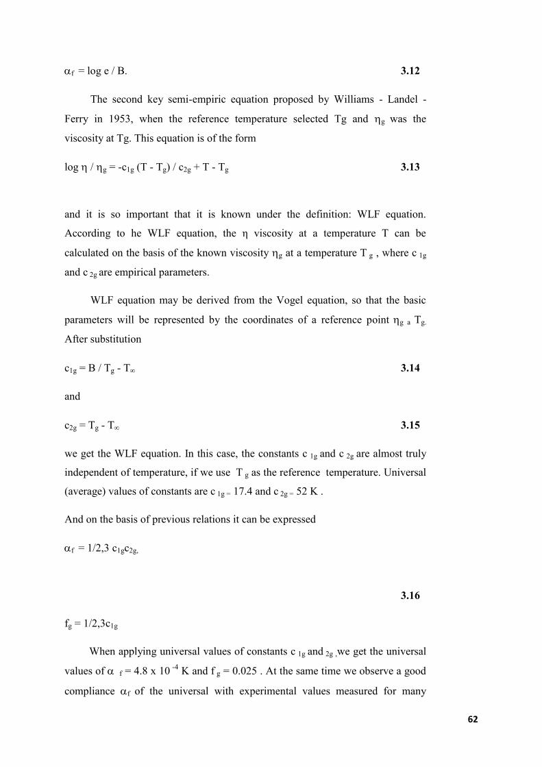
62

f = log e / B. 3.12

The second key semi-empiric equation proposed by Williams - Landel -

Ferry in 1953, when the reference temperature selected Tg and g was the

viscosity at Tg. This equation is of the form

log / g = -c1g (T - Tg) / c2g + T - Tg 3.13

and it is so important that it is known under the definition: WLF equation.

According to he WLF equation, the η viscosity at a temperature T can be

calculated on the basis of the known viscosity g at a temperature T g , where c 1g

and c 2g are empirical parameters.

WLF equation may be derived from the Vogel equation, so that the basic

parameters will be represented by the coordinates of a reference point g a Tg.

After substitution

c1g = B / Tg - T 3.14

and

c2g = Tg - T 3.15

we get the WLF equation. In this case, the constants c 1g and c 2g are almost truly

independent of temperature, if we use T g as the reference temperature. Universal

(average) values of constants are c 1g = 17.4 and c 2g = 52 K .

And on the basis of previous relations it can be expressed

f = 1/2,3 c1gc2g,

3.16

fg = 1/2,3c1g

When applying universal values of constants c 1g and 2g ,we get the universal

values of f = 4.8 x 10 -4

K and f g = 0.025 . At the same time we observe a good

compliance f of the universal with experimental values measured for many

63

polymers. Also, from the definition for f g it implies that at T g the free volume is

2.5% of the total volume of body, i.e. 97.5 % are occupied by matters of

molecules. When temperature rises by 100 o

C above T g, the parameter fg will

reach a value of 0.075 g , i.e. , the free volume will be increased to 7.5 %.

This result can be interpreted also in a way that under T g the free volume is

virtually constant. In this case, the measured thermal expansion of a material in a

vitreous condition will be only the measure of the expansion of molecules itself.

Based on the considerations of Simha and Boyer, the volume of molecules Vm can

be obtained at absolute zero by extrapolation from the liquid.

As it was said above, T g is formally the transition of the 2nd order . From

the thermodynamic standpoint, however, this claim is not quite accurate, because

the measurements of thermodynamic quantities in the environment of T g are not

at equilibrium, but the time factor (the rate of temperature change) plays a role

here, as well as the history of a sample (the method for preparation). Therefore, T

g cannot be considered as a thermodynamically defined transition. The result is the

fact that the experimental determination of T g for a specific polymer depends on

the method used, and to some extent on the conditions of the experiment.

Therefore, within the professional literature the mentioned values T g differ,

sometimes by more than dozens of o

C .

Thermodynamic theory, which was presented by Gibbs and Di Marzio, says

that the equilibrium transition actually exists and it is situated in the surroundings

of Vogel temperatureT. In practice, however, these measurements are

impracticable, because it would require infinitely slow changes in temperature. A

relatively reliable picture can be obtained using a grid-model, with which we can

calculate a conformational energy system and conformational entropy. With

decreasing temperature, the number of viable macro-conformations reduces, while

of course the energy-poorer conformation prevail. At the limit temperature of

absolute zero in a perfectly frozen condition all macro-conformations should be

trans, the number of possible statuses would be 1 and conformational entropy

zero. Real systems freeze several tens of degrees above this temperature, where

the number of conformational transitions is small and transitions rare.

64

3.2. Models of viscous elastic materials

Let us now follow the issue of viscous environment phenomenologically.

For elastic environment, as we already know, Hook´s law applies in its symbolic

form

σ=Eε . 3.17

Newton´s law of viscous creep can be written as

σ = η ε’, 3.18

where ε’ represents the strain rate.

Equation 3.18 does not describe distortions causing changes in volume during a

deformation of the environment, but it only describes shear deformation.

Nevertheless, in the dissemination of the elastic waves in viscous environments,

under certain conditions deformations of volume and the consequent contribution

to viscosity environment arise, also called bulk viscosity η'.

The real environment, as we have said, has viscous and elastic properties.

Measured time dependence of the shear deformation, as shown in Figure 3.6a, we

can therefore divide into three components, namely elastic, viscous, and relaxation

(Figure 3.6b, c, d).

Let us suppose that the stress is composed of the 'flexible stress" σ E and

from "viscous stress" σ η

'

ηE 'ηε+εE=σ+σ=σ 3.19

This equation is also called Kelvin´s equation.

If, at the time t=0 we apply the rectangular pulse of the mechanical tension T0 to

such an environment, then the environment will be described by relations

( )E

η=τ;e-1

E

σ=ε τ/t0

. 3.20

65

Figure 3. 6. Experimental time-dependent shear deformation (a). Distribution

of deformation into flexible (b), viscous (c), and relaxation component (d)

For a sufficiently long time in the environment there is created a time-

independent constant deformation E

σ=ε

0

∞ and the environment acts as non-

viscous . Reaction of the environment to the applied stress is probably not

immediate, but it progressively achieves the maximum value. Similarly, after

an interruption of the stress, this deformation exponentially decreases to zero,

while the time of relaxation is determined by the relationshipE

η=τ . This type

of deformation is called the delayed deformation.

Another approach to describe a viscous elastic environment was used by

Maxwell, who anticipated that within the environment two types of

deformations occur, elastic and viscous.

ε=εE+εη . 3.21

After derivation 3.6 by time and the substitution from relations 3.2 and 3.3 we

get

η

σ+

E

σ=ε

'

'. 3.22

From this equation it is clear that this deformation is composed of a

deformation proportional to the stress and viscous creep.

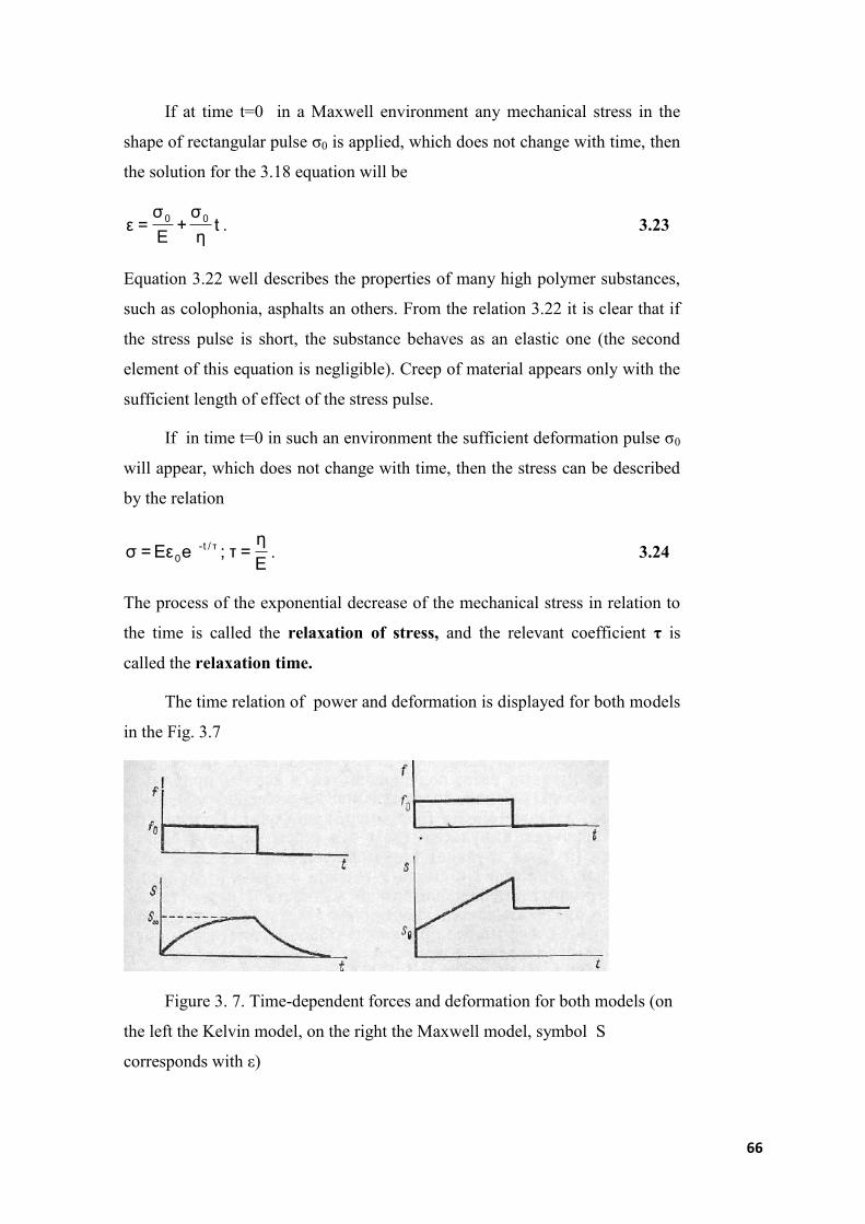
66

If at time t=0 in a Maxwell environment any mechanical stress in the

shape of rectangular pulse σ0 is applied, which does not change with time, then

the solution for the 3.18 equation will be

tη

σ+

E

σ=ε

00. 3.23

Equation 3.22 well describes the properties of many high polymer substances,

such as colophonia, asphalts an others. From the relation 3.22 it is clear that if

the stress pulse is short, the substance behaves as an elastic one (the second

element of this equation is negligible). Creep of material appears only with the

sufficient length of effect of the stress pulse.

If in time t=0 in such an environment the sufficient deformation pulse σ0

will appear, which does not change with time, then the stress can be described

by the relation

E

η=τ;eεE=σ τ/t-

0 . 3.24

The process of the exponential decrease of the mechanical stress in relation to

the time is called the relaxation of stress, and the relevant coefficient τ is

called the relaxation time.

The time relation of power and deformation is displayed for both models

in the Fig. 3.7

Figure 3. 7. Time-dependent forces and deformation for both models (on

the left the Kelvin model, on the right the Maxwell model, symbol S

corresponds with ε)

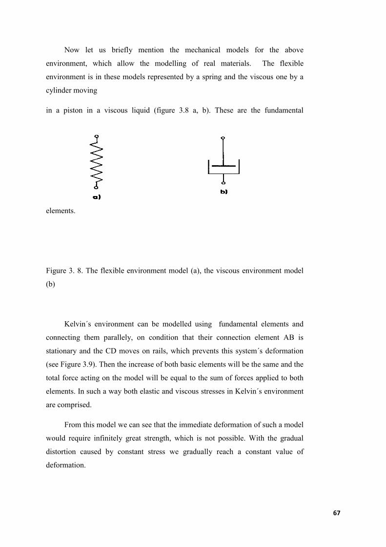
67

Now let us briefly mention the mechanical models for the above

environment, which allow the modelling of real materials. The flexible

environment is in these models represented by a spring and the viscous one by a

cylinder moving

in a piston in a viscous liquid (figure 3.8 a, b). These are the fundamental

elements.

Figure 3. 8. The flexible environment model (a), the viscous environment model

(b)

Kelvin´s environment can be modelled using fundamental elements and

connecting them parallely, on condition that their connection element AB is

stationary and the CD moves on rails, which prevents this system´s deformation

(see Figure 3.9). Then the increase of both basic elements will be the same and the

total force acting on the model will be equal to the sum of forces applied to both

elements. In such a way both elastic and viscous stresses in Kelvin´s environment

are comprised.

From this model we can see that the immediate deformation of such a model

would require infinitely great strength, which is not possible. With the gradual

distortion caused by constant stress we gradually reach a constant value of

deformation.

68

Figure 3.9. Model of Kelvin´s environment

Maxwell´s environment can be modelled using the series connections of

basic elements, as seen in Figure 3. 10. In this case the same force acts on both

elements and their extensions are composite

Figure 3. 10. Model of the Maxwell´s environment

Real viscous elastic environments are behaving in a more complex way. One of

the models is the so-called Knezer´s model shown in Figures 3. 11.

In Figure 3.12 the flow curve of a rubber mixture is shown, which is qualitatively

very similar to Knezerś model.

69

On the basis of acquired knowledge we can now define a comprehensive

Young's modulus, which is described schematically in Figure 3.13, and from

which we get that the viscous elastic properties of a viscous model are

described by the imaginary part of this module and by the elastic real part

of the module.

Figure 3. 11. Knezer´s model (left diagram, right time course of the force and

deformation)

.

Figure 3. 12. The flow curve of the rubber mixture

70

Figure 3.13. Complex Young's modulus

Module and the viscosity are thus frequency-dependent, which is typical

for the viscous elastic materials.

The operator of the effective module will have in Maxwell´s environment the

shape

dt

dτ+1

dt

dη

=E . 3.25

For the harmonic signal we get

i1

iE .

If we divide the expression for the effective module into its real and imaginary

parts, we get

2222

22

1i

1EE

. 3.26

Quantity

E1

EERe

22

22

3.27

is called the dynamic module.

221EIm

1 3.28

is called the dynamic viscosity.

From relations 3.26 and 3.27 we can see that at low frequencies (ωτ<< 1)

Maxwell´s environment acts as a viscous liquid, because its dynamic module is

very small and its dynamic viscosity is frequency-independent. With the

growth of its frequency the dynamic viscosity begins to fall, the dynamic

module is growing, and for very high frequencies (ωτ>>1) Maxwell´s

environment acts like a solid. This process is called the relaxation of viscosity

.

71

In the case of Kelvin´s environment the dynamic module and its dynamic

viscosity are frequency-independent.

3.3 Payne effect

Adding some filler to a polymeric matrix significantly affects the behaviour

of individual dynamic characteristics depending on increasing the instance of the

dynamic deformation, with regard to the quality of interactions established

between the particles in the fillers themselves, and between the particles in a filler

and the polymer matrix. The quality of these interactions can be assessed by

measuring the dynamic-mechanic properties of the prepared composites at various

amplitudes of the dynamic deformation.

The values of the elastic module (E') for not filled vulcanizates do not change

significantly with a raising level of dynamic distortion; in the case of stuffed

vulcanizates, however, there is a decrease in the module, and this effect is more

pronounced for vulcanizates with a higher content of filler. This phenomenon is

called the Payne effect.

In the case of a leaking module (E' ), like in the case of the elastic module,

the increase of its values with the increasing degree of polymer filling in a whole

range of dynamic distortions is observed. Depending on the increase in

deformation, however, there are no monotonous value decreases observed, as in

the case of an elastic module, but the maximum at a certain deformation,

characteristic for a given pair of the polymer-filler. It is assumed that the

development of the loss module is controlled by extinction and the recovery

of the filler particles networks. Consequently, the loss module is dependent on

the speed of extinction and recovery of the network. The speed of extinction and

recovery of the network is based on the dynamic deformation phenomenon. When

the distortion is large, the disappearance of a network is significant, and its

recovery practically does not occur. If the deformation is sufficiently large for the

network to recover at a given frequency, the impact of the network on the loss

module will be eliminated.

72

Similarly, if a deformation is small (or the network is sufficiently strong) to

trigger the extinction of a network, the loss module is not dependent on the given

deformation, but it will mainly depend on the contribution of the polymeric matrix

during the cyclic dynamic deformations of the composite.

A change of each of the modules (elastic and loss) depending on the size of

dynamic distortion is based on other mechanisms. While an elastic module

depends to a large extent on the presence of a physical network (its gradual

disappearance in with the increasing dynamic deformation) consisting of

filler particles in a polymeric matrix, the loss-making module is affected by

the repeated process of dissolution and the recovery of its structure during

the cyclical stress.

The polymer-filler interaction causes the absorption of the polymer chains to

the surface of the filler, thus limiting the mobility of the polymer segments. The

result is the creation of a polymeric layer on the filler surface, where the

viscosity and the module of polymer will increase. A very high module in

proximity to the surface of the filler particles within the polymer shell with an

increasing distance from the surface filler will fall, until at a certain distance it

will be the same as the module for the polymer matrix. If there are two or more

particles of the filler or units which are close together enough, they create an

agglomerate of a mechanism of mutual breaches of the polymer shells in filler

particles. The network, set up using such a mechanism, will be less rigid than the

network, set up using a direct contact between the aggregates. This type of

network can begin to fade already at relatively small deformations.

In the case of a network created by the direct contact of aggregates the

process of repeated extinction and subsequent recovery of a network causes

higher loss energy. This shows that at high temperatures the internal friction

between the aggregates is the dominant mechanism. When reducing

temperature, the polymer gets into the glass transition area, where the

polymer mix has the major proportion of the losses of the included

mechanical energy.

If the network consists of the mutually breached shells of particles, the

mechanism of contribution to the energy losses is different than the one for the

73

network described above. At higher temperatures the polymer matrix is in a

rubber condition, but the polymer adsorbed on the filler surface is in the

phase of transition. This leads us to the fact that the shell can absorb more

energy. As the temperature increases, the thickness of the shell decreases, which

increases the mobility of chains, which leads to a lower hysteresis. Reversed re-

agglomeration of the filler during cyclic dynamic deformation reaches a higher

degree.

The most significant impact on the dynamic properties changes of

polymers is represented by the morphology of the filler particle, namely the

size of particles or their specific surface, and particles structure. With an

increasing specific surface of the soot at the constant replacement, a sharper

decrease in the elastic module is observed, with an increasing degree of the

dynamic deformation. An increase in the Payne effect indicates the great ability of

small particles (aggregates) in soot to agglomerate in a polymeric matrix.

From these considerations it is clear that the measurements of the

Payne effect may contribute significantly to the characterisation of

interactions between the components of the filled vulcanizate in the dynamic

conditions.

We will monitor the Payne effect on the developments of the dynamic

characteristics of polymers with a different content of fillers, according to the

degree of the dynamic deformation.

The addition of filler into the polymeric matrices in general affects the

increase of elastic module values, which is caused by the nature of a filler,

which behaves as a Hook´s element. By comparing the values of modules for a

given temperature, frequency, the amplitude of distortion, and the selection of a

pair polymer matrix - we can see that the values of modules grow with the degree

of filling .

In Figures 3.14 and 3.15 there are displayed the dependences of modules of

E and G for the tread mixture. It is visible that even during the static

measurements of elastic modules the Payne effect is demonstrated by a decrease

in the values for both modules.

74

Figure 3.14. Dependence of Young´s modulus on the perpendicular

operating pressure

Figure 3 15. Dependence of the shearing module on perpendicularly

operating pressure

Summary of terms

Transformation of coordinates and tensors, properties of the second-order tensors,

stress tensors, distortions and Hook´s law in general form, compressibility, the impact of

lattice symmetry on the the number of independent components of the tensor.

1.Define Newton's liquid.

2. Qualitatively describe the material flow from a microscopic point of view.

75

3. What is entropic flexibility?

4. Describe the glass stage conditions.

5. What equations describe the glass transition in polymers?

6. Explain Kelvin´s model.

7. Explain Maxwell´s model.

8. Explain Knezer´s model.

9. Explain the fundamentals of the complex Young´s model.

10. Explain Payne phenomenon.

Questions to the topic

1. How to transform the second-order tensor?

2. What relationship determines the stress tensor constituents?

3. Explain Hook´s law in its general form.

4. How can we calculate the compressibility of anisotropic material?

5. What is the impact of symmetry on the number of independent components of the second-

order tensor?

6. Explain the term invariant tensor, and what it determines?

76