Solitons and instantons in gauge theories - cvut.cz · Solitons and instantons in gauge theories⁄ Petr Jizba FNSPE, Czech Technical University, Prague, Czech Republic ITP, Freie

Solitons and instantons in gauge theories∗

Petr Jizba

FNSPE, Czech Technical University, Prague, Czech Republic

ITP, Freie Universitat Berlin, Germany

March 15, 2007

∗From: M. Blasone, PJ and G. Vitiello,Quantum Field Theory and its Macroscopic Manifestations (WS, 2007)

Praha, 15.3.2007

1

Outlook:

2

Outlook:

•

2

Outlook:

• Introduction & motivations

2

Outlook:


• Korteweg–de Vries solitons

2

Outlook:



• Topological solitons in 1 + 1 relativistic field theories

2

Outlook:




−

2

Outlook:




− sine-Gordon solitons

2

Outlook:





−

2

Outlook:





− φ4 solitary waves

2

Outlook:






• Topological solitons in gauge theories with SSB

2

Outlook:







−

2

Outlook:







− Nielsen–Olesen vortex solution

2

Outlook:








−2

Outlook:








− ’t Hooft–Polyakov magnetic monopole solution2

Outlook:








− ’t Hooft–Polyakov magnetic monopole solution

•2

Outlook:








− ’t Hooft–Polyakov magnetic monopole solution

• Homotopy theory and soliton classification2

Introduction & motivation

In QM bound states describe extended structures (nucleons, atoms,

molecules) that are inherently quantum (they are stable against radi-

ation only in the QM setting).

3





Q.:

3





Q.: Can we have stable bound states in (relativistic) QFT which are

not inherently quantum?

3







A:

3







A: Yes. In a non-linear field theory, with an“appropriate” amount of

non-linearity, stable bound states can exist on a classical, as well

as quantum level. Such bound states are called solitons.

3







A: Yes. In a non-linear field theory, with an“appropriate” amount of

non-linearity, stable bound states can exist on a classical, as well

as quantum level. Such bound states are called solitons.

⇒ solitons can be viewed as elementary objects in much the same way

as elementary particles are (sol. are stabilized by topological charge).

3

Other properties

•

4

Other properties

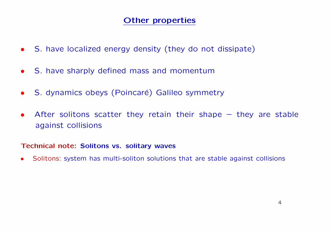
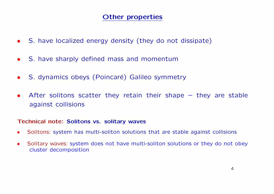
• S. have localized energy density (they do not dissipate)

4

Other properties


• S. have sharply defined mass and momentum

4

Other properties



• S. dynamics obeys (Poincare) Galileo symmetry

4

Other properties




• After solitons scatter they retain their shape – they are stable

against collisions

4

Other properties





against collisions

Technical note: Solitons vs. solitary waves

4

Other properties





against collisions


•

4

Other properties





against collisions


• Solitons: system has multi-soliton solutions that are stable against collisions

4

Other properties





against collisions


• Solitons: system has multi-soliton solutions that are stable against collisions

• Solitary waves: system does not have multi-soliton solutions or they do not obeycluster decomposition

4

Korteweg–de Vries solitons

5

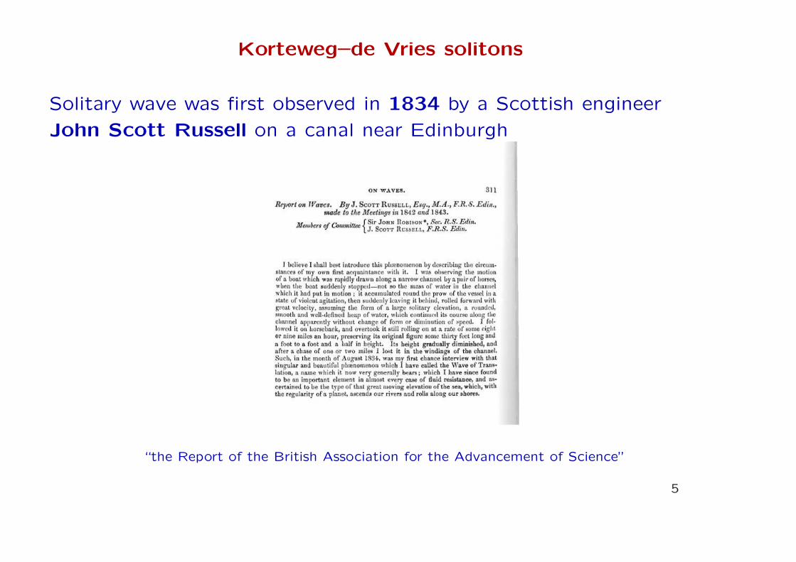
Korteweg–de Vries solitons

Solitary wave was first observed in 1834 by a Scottish engineer

John Scott Russell on a canal near Edinburgh

“the Report of the British Association for the Advancement of Science”

5

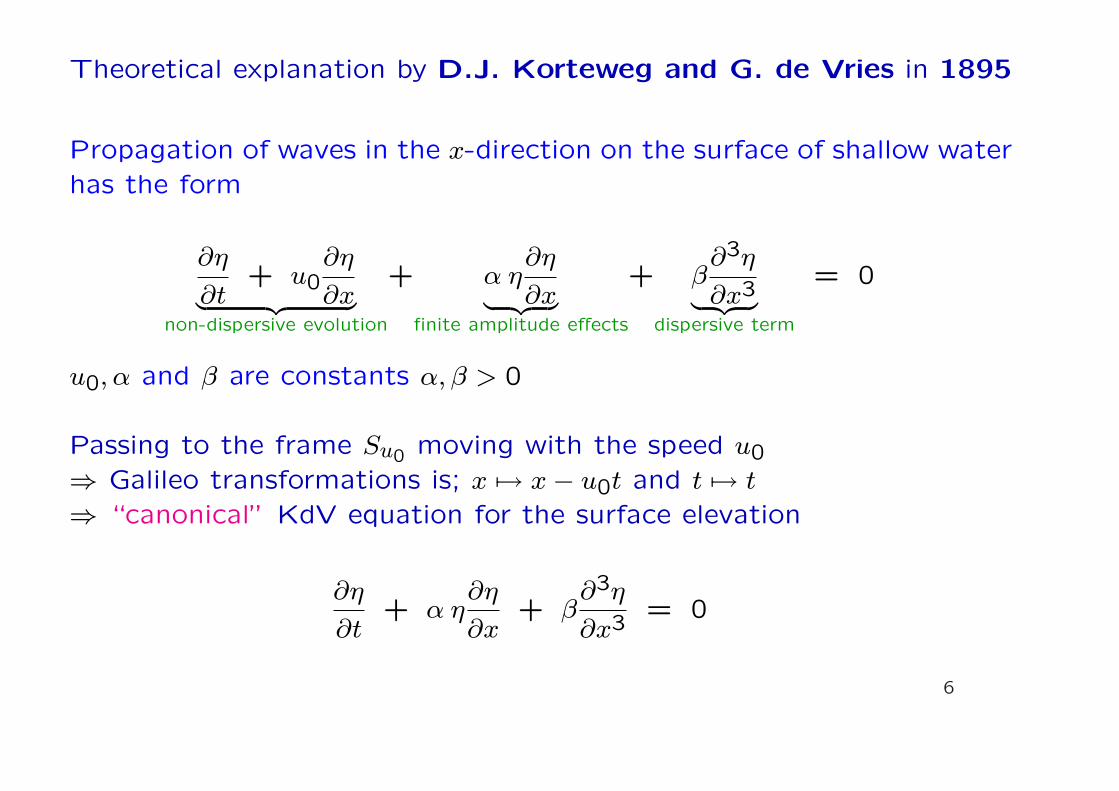
Theoretical explanation by D.J. Korteweg and G. de Vries in 1895

Propagation of waves in the x-direction on the surface of shallow waterhas the form

∂η

∂t+ u0

∂η

∂x︸︷︷︸non-dispersive evolution

+ α η∂η

∂x︸︷︷︸finite amplitude effects

+ β∂3η

∂x3︸︷︷︸dispersive term

= 0

u0, α and β are constants α, β > 0

Passing to the frame Su0 moving with the speed u0

⇒ Galileo transformations is; x 7→ x− u0t and t 7→ t

⇒ “canonical” KdV equation for the surface elevation

∂η

∂t+ α η

∂η

∂x+ β

∂3η

∂x3= 0

6

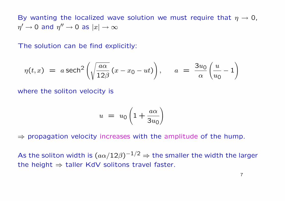
By wanting the localized wave solution we must require that η → 0,

η′ → 0 and η′′ → 0 as |x| → ∞

The solution can be find explicitly:

η(t, x) = a sech2(√

aα

12β(x− x0 − ut)

), a =

3u0

α

(u

u0− 1

)

where the soliton velocity is

u = u0

(1 +

aα

3u0

)

⇒ propagation velocity increases with the amplitude of the hump.

As the soliton width is (aα/12β)−1/2 ⇒ the smaller the width the larger

the height ⇒ taller KdV solitons travel faster.

7

Note: The localized behavior results from a balance between nonlin-ear steepening and dispersive spreading and so it cannot be attainedin linear equations because an appropriate amount of nonlinearity isnecessary.

!!! KdV equation allows for a superposition of solitons and hence itcan describe an interaction between solitons.

Numerical investigations of the interaction of two solitons reveal thatif a high, narrow soliton is formed behind a low, broad one, it willcatch up with the low one, they undergo a non-linear interaction —the high soliton passes through the low one — and both emerge withtheir shape unchanged.

Note: KdV equation can be generalized. Ensuing equations are calledhigher-order KdV equations and they have form

∂η

∂t+ u0

∂η

∂x+ (p + 1)ηp∂η

∂x+

∂3η

∂η3= 0 , p ≥ 2

8

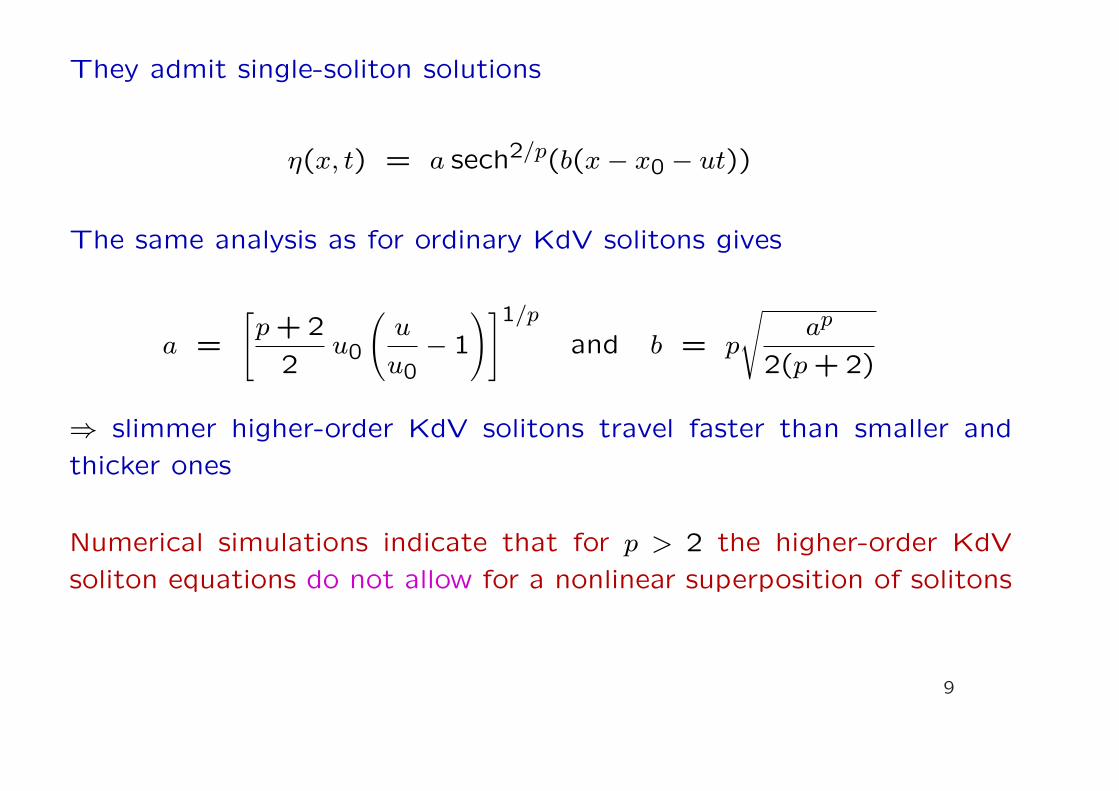
They admit single-soliton solutions

η(x, t) = a sech2/p(b(x− x0 − ut))

The same analysis as for ordinary KdV solitons gives

a =

[p + 2

2u0

(u

u0− 1

)]1/p

and b = p

√ap

2(p + 2)

⇒ slimmer higher-order KdV solitons travel faster than smaller and

thicker ones

Numerical simulations indicate that for p > 2 the higher-order KdV

soliton equations do not allow for a nonlinear superposition of solitons

9

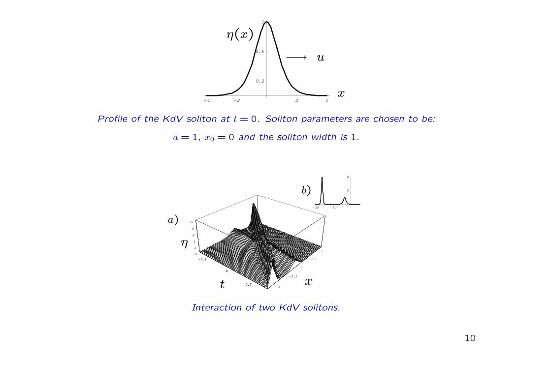
-4 -2 2 4

0.2

0.6

1

Profile of the KdV soliton at t = 0. Soliton parameters are chosen to be:

a = 1, x0 = 0 and the soliton width is 1.

−→ u

η(x)

x

-0.2

0

0.2-5

-2.5

0

2.5

5

0

2

4

6

8

10

-0.2

0

0.2

-20 -10

4

8

Interaction of two KdV solitons.

b)

a)

xt

η

10

Topological solitons in 1 + 1 relativistic field theories

Important class of systems which often exhibit solitonic solutions are1 + 1 dimensional relativistic field theories.

For the single scalar field φ the Lagrangians reads

L =1

2(φ)2 − 1

2(φ′)2 − V (φ)

and the corresponding E–L equation is

φ − φ′′ = −dV (φ)

dφ

The energy is obtained from the 00 component of the E-M tensor ⇒

E[φ] =∫

dx T00(φ) =∫

dx

(1

2(φ)2 +

1

2(φ′)2 + V (φ)

)

11

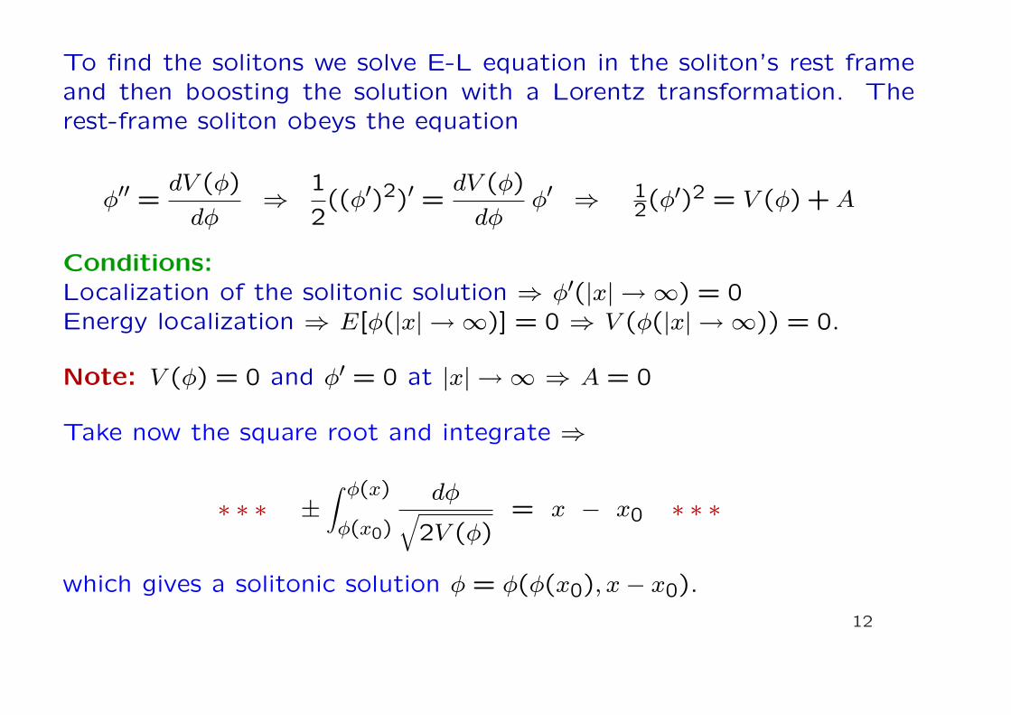
To find the solitons we solve E-L equation in the soliton’s rest frameand then boosting the solution with a Lorentz transformation. Therest-frame soliton obeys the equation

φ′′ = dV (φ)

dφ⇒ 1

2((φ′)2)′ = dV (φ)

dφφ′ ⇒ 1

2(φ′)2 = V (φ) + A

Conditions:Localization of the solitonic solution ⇒ φ′(|x| → ∞) = 0Energy localization ⇒ E[φ(|x| → ∞)] = 0 ⇒ V (φ(|x| → ∞)) = 0.

Note: V (φ) = 0 and φ′ = 0 at |x| → ∞ ⇒ A = 0

Take now the square root and integrate ⇒

∗ ∗ ∗ ±∫ φ(x)

φ(x0)

dφ√2V (φ)

= x − x0 ∗ ∗ ∗

which gives a solitonic solution φ = φ(φ(x0), x− x0).

12

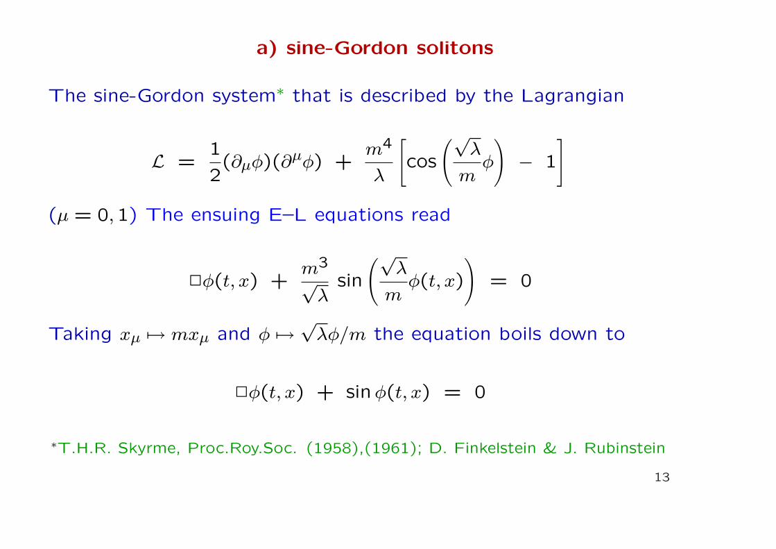
a) sine-Gordon solitons

The sine-Gordon system∗ that is described by the Lagrangian

L =1

2(∂µφ)(∂µφ) +

m4

λ

[cos

(√λ

mφ

)− 1

]

(µ = 0,1) The ensuing E–L equations read

2φ(t, x) +m3√

λsin

(√λ

mφ(t, x)

)= 0

Taking xµ 7→ mxµ and φ 7→ √λφ/m the equation boils down to

2φ(t, x) + sinφ(t, x) = 0

∗T.H.R. Skyrme, Proc.Roy.Soc. (1958),(1961); D. Finkelstein & J. Rubinstein

13

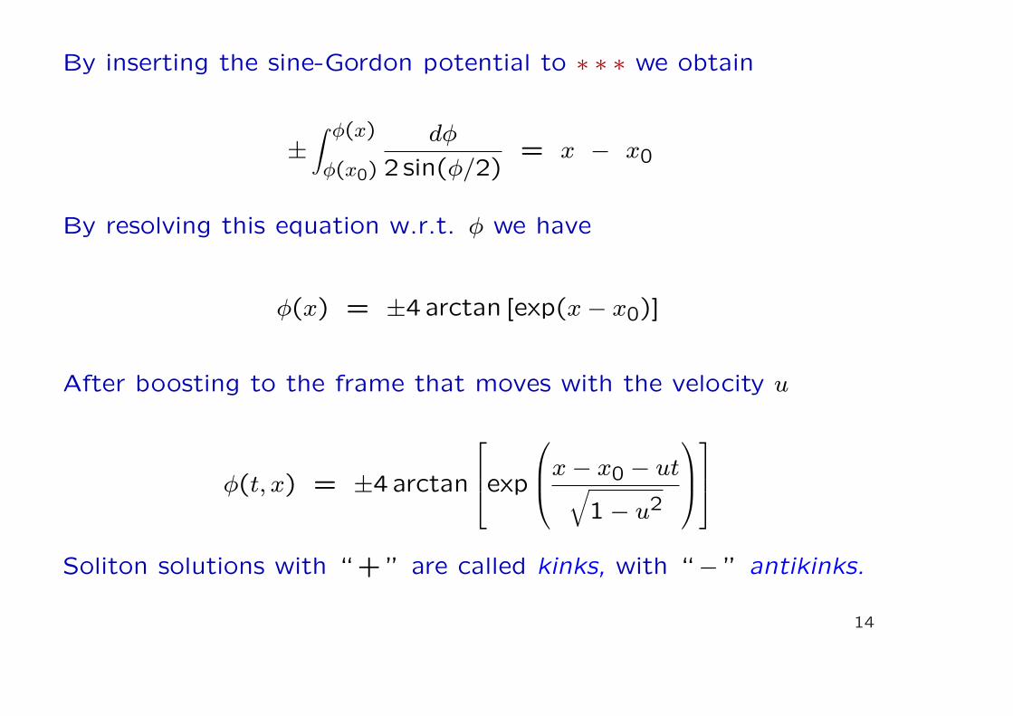
By inserting the sine-Gordon potential to ∗ ∗ ∗ we obtain

±∫ φ(x)

φ(x0)

dφ

2 sin(φ/2)= x − x0

By resolving this equation w.r.t. φ we have

φ(x) = ±4arctan [exp(x− x0)]

After boosting to the frame that moves with the velocity u

φ(t, x) = ±4arctan

exp

x− x0 − ut√1− u2

Soliton solutions with “ + ” are called kinks, with “− ” antikinks.

14

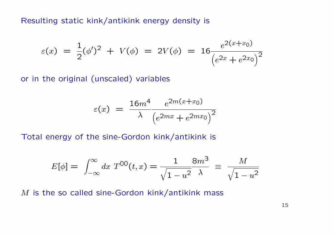
Resulting static kink/antikink energy density is

ε(x) =1

2(φ′)2 + V (φ) = 2V (φ) = 16

e2(x+x0)

(e2x + e2x0

)2

or in the original (unscaled) variables

ε(x) =16m4

λ

e2m(x+x0)

(e2mx + e2mx0

)2

Total energy of the sine-Gordon kink/antikink is

E[φ] =∫ ∞−∞

dx T00(t, x) =1√

1− u2

8m3

λ≡ M√

1− u2

M is the so called sine-Gordon kink/antikink mass

15

-6 -4 -2 2 4 6

3

6

-6 -4 -2 2 4 6

2

4

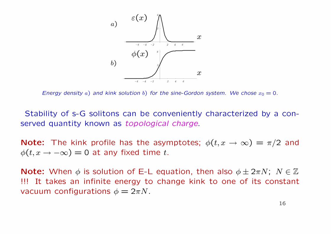
Energy density a) and kink solution b) for the sine-Gordon system. We chose x0 = 0.

b)

a)

x

x

ε(x)

φ(x)

Stability of s-G solitons can be conveniently characterized by a con-served quantity known as topological charge.

Note: The kink profile has the asymptotes; φ(t, x → ∞) = π/2 andφ(t, x → −∞) = 0 at any fixed time t.

Note: When φ is solution of E-L equation, then also φ± 2πN ; N ∈ Z!!! It takes an infinite energy to change kink to one of its constantvacuum configurations φ = 2πN .

16

As S. are finite-energy solutions they must at x → ±∞ tend towardsone of vacua, labeled by N ⇒ define the conserved charge Q as

Q =∫ ∞−∞

dx J0(t, x) ≡ 1

2π

∫ ∞−∞

dx φ′(t, x)

=1

2π[φ(t, x →∞) − φ(t, x → −∞)] = N2 − N1

N1 and N2 are integers corresponding to asymptotic values of the field.Jµ that satisfies the continuity equation can be defined as

Jµ(t, x) =1

2πεµν∂νφ(t, x)

(εµν is the 2-dimensional Levi–Civita tensor)

Q = const. ⇒ S. with one Q cannot evolve into S. with a different Q.

Note: Topological charge Q cannot be derived from Noether’s theoremsince it is not related to any continuous symmetry of the Lagrangian.

17

b) φ4 solitary waves

For small field elevations, we can expand in s-G sin(. . .) up to the thirdorder. After rescaling λ/3! to λ the resulting E–L equation is

2φ(t, x) + m2φ(t, x) − λφ3(t, x) = 0

Ensuing Lagrange density can be written as

L =1

2(∂µφ)(∂µφ) − λ

4

(φ2 − m2

λ

)2

Inserting the V (φ) into ∗ ∗ ∗ ⇒ static kink equation

±∫ φ(x)

φ(x0)

dφ√λ2

(φ2 − m2

λ

) = x − x0

18

⇒

φ(x) = ± m√λ

tanh

[m√2(x− x0)

]

The boosted solution then reads

φ(t, x) = ± m√λ

tanh

m√2

(x− x0 − ut)√1− u2

One calls solutions with “ + ” as kinks and “ − ” sign solutions asantikinks. Resulting kink/antikink energy density T00 is

T00(t, x) =1

2(φ)2 +

1

2(φ′)2 + V (φ)

=m4

2λ(1− u2)sech4

m√2

(x− x0 − ut)√1− u2

19

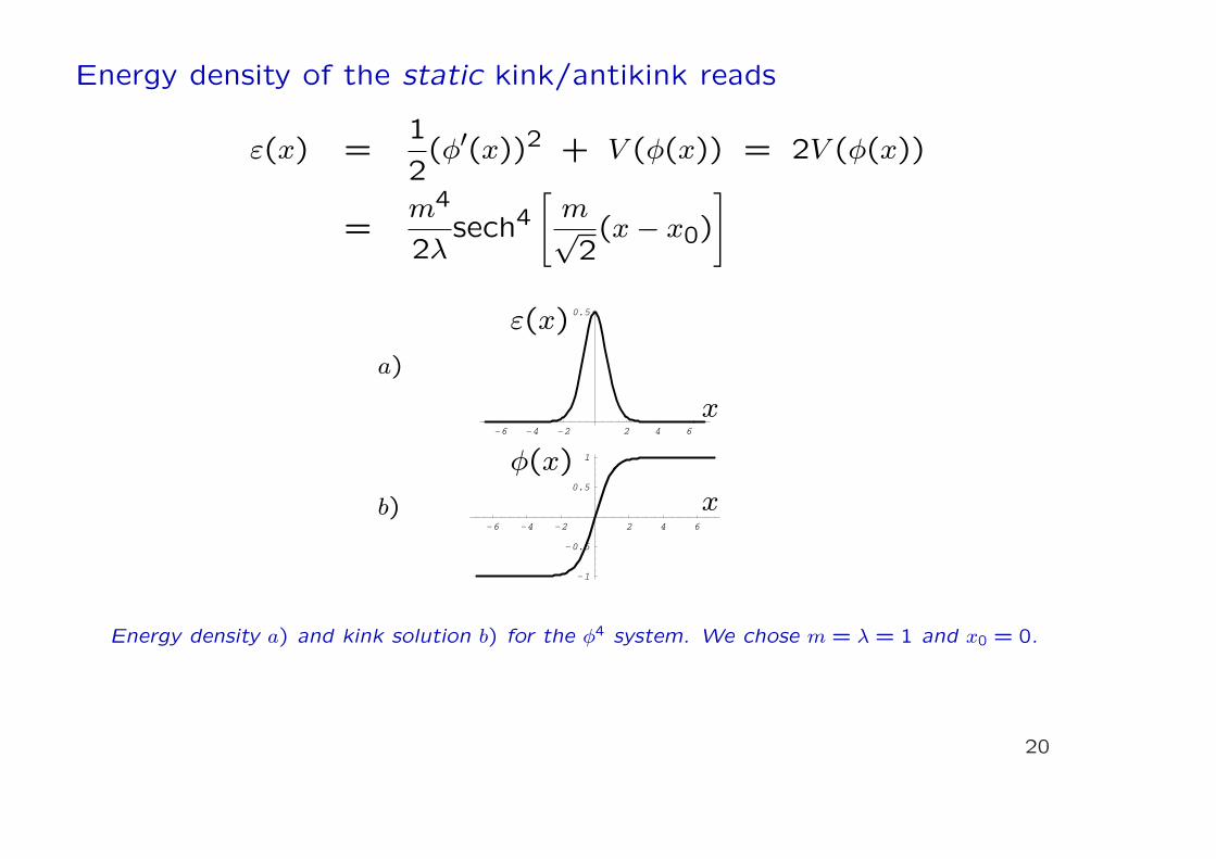
Energy density of the static kink/antikink reads

ε(x) =1

2(φ′(x))2 + V (φ(x)) = 2V (φ(x))

=m4

2λsech4

[m√2(x− x0)

]

-6 -4 -2 2 4 6

-1

-0.5

0.5

1

-6 -4 -2 2 4 6

0.5

Energy density a) and kink solution b) for the φ4 system. We chose m = λ = 1 and x0 = 0.

b)

a)

x

x

ε(x)

φ(x)

20

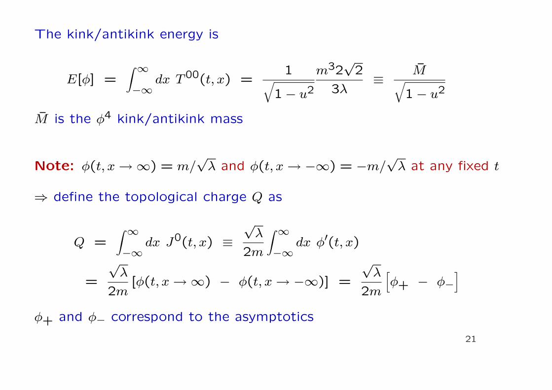
The kink/antikink energy is

E[φ] =∫ ∞−∞

dx T00(t, x) =1√

1− u2

m32√

2

3λ≡ M√

1− u2

M is the φ4 kink/antikink mass

Note: φ(t, x →∞) = m/√

λ and φ(t, x → −∞) = −m/√

λ at any fixed t

⇒ define the topological charge Q as

Q =∫ ∞−∞

dx J0(t, x) ≡√

λ

2m

∫ ∞−∞

dx φ′(t, x)

=

√λ

2m[φ(t, x →∞) − φ(t, x → −∞)] =

√λ

2m

[φ+ − φ−

]

φ+ and φ− correspond to the asymptotics

21

The associated topological current Jµ can be defined as

Jµ(t, x) =

√λ

2mεµν∂νφ(t, x)

⇒ possible values of Q are {−1,0,1}

Note: Values |N | > 1 are not a allowed because the corresponding

field configurations do not have boundary conditions compatible with

the finite energy

⇒ no multi-solitonic solutions with |N | > 1 can exist

Note: Field configurations containing a finite mixture of kinks and

antikinks alternating along the x-direction preserving N = {−1,0,1}can be (numerically) constructed

but there are no static solutions of this type

22

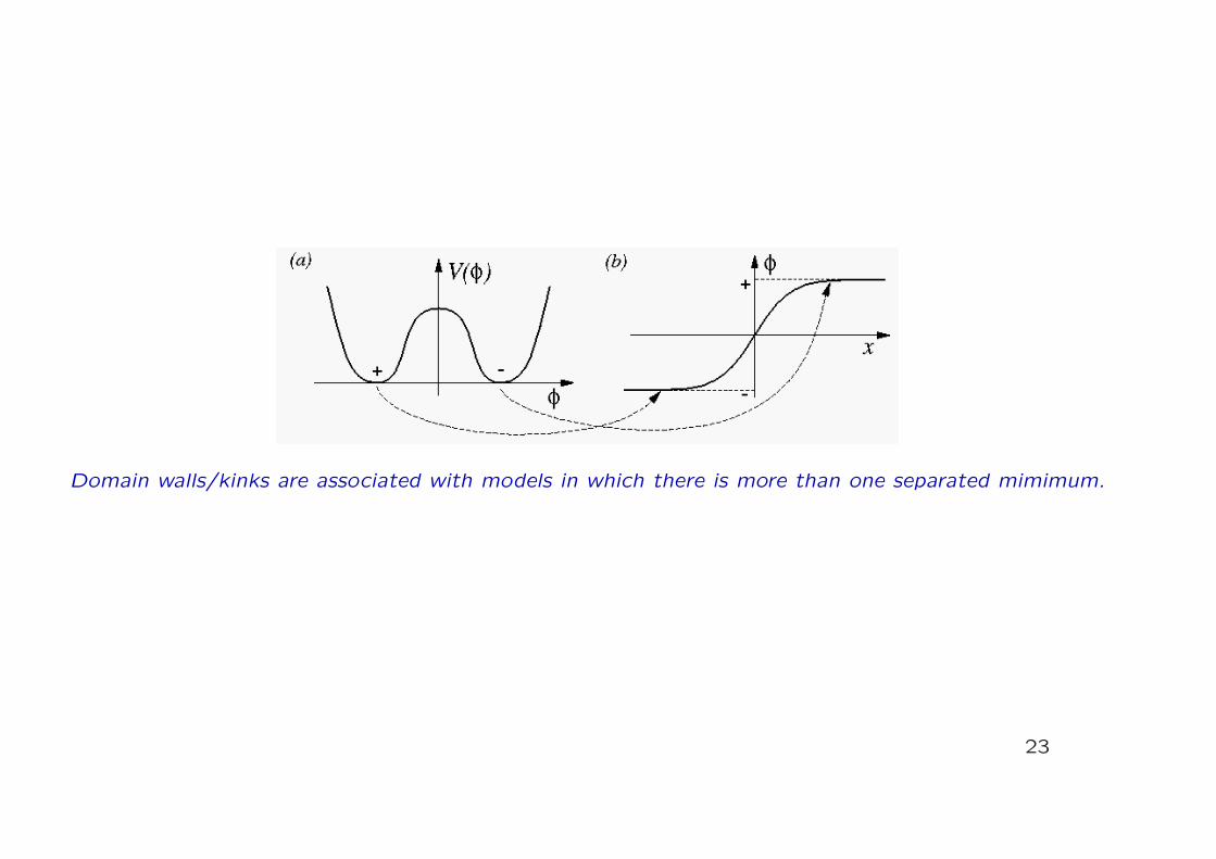
Domain walls/kinks are associated with models in which there is more than one separated mimimum.

23

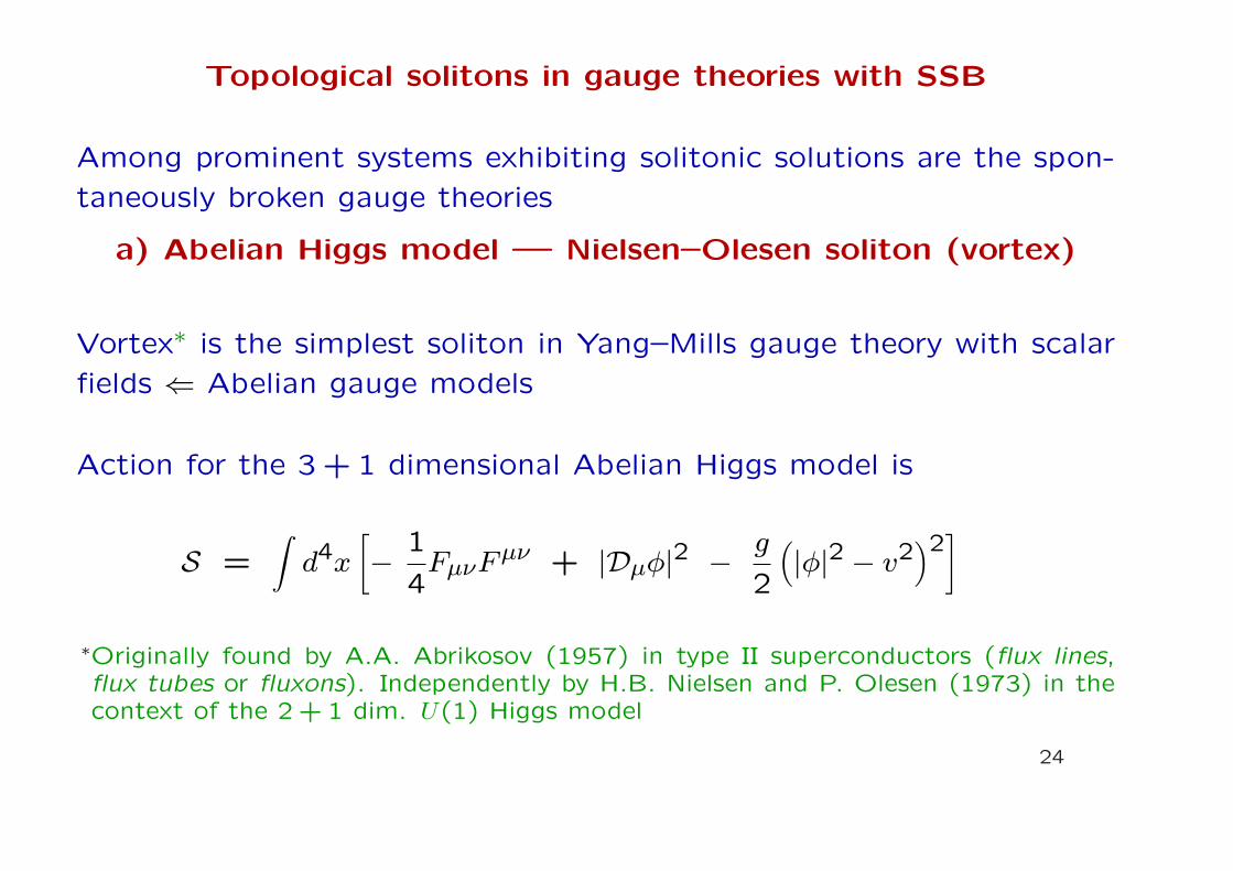
Topological solitons in gauge theories with SSB

Among prominent systems exhibiting solitonic solutions are the spon-

taneously broken gauge theories

a) Abelian Higgs model — Nielsen–Olesen soliton (vortex)

Vortex∗ is the simplest soliton in Yang–Mills gauge theory with scalar

fields ⇐ Abelian gauge models

Action for the 3 + 1 dimensional Abelian Higgs model is

S =∫

d4x

[− 1

4FµνFµν + |Dµφ|2 − g

2

(|φ|2 − v2

)2]

∗Originally found by A.A. Abrikosov (1957) in type II superconductors (flux lines,flux tubes or fluxons). Independently by H.B. Nielsen and P. Olesen (1973) in thecontext of the 2 + 1 dim. U(1) Higgs model

24

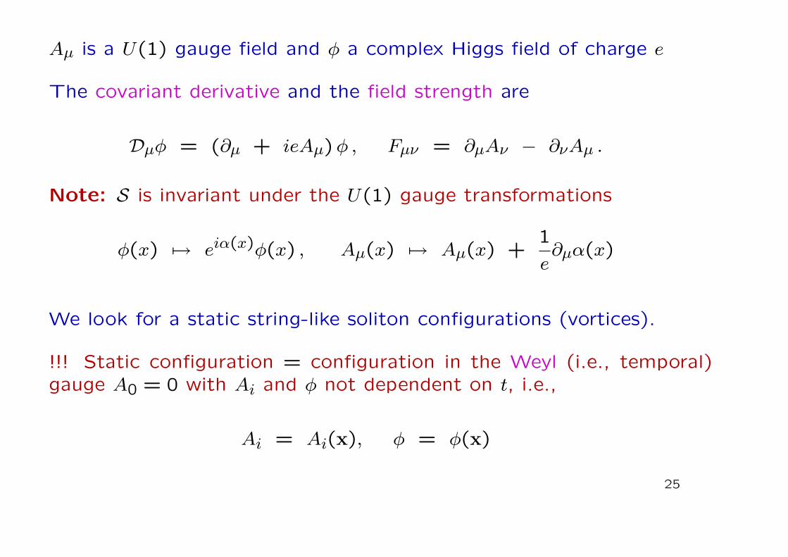
Aµ is a U(1) gauge field and φ a complex Higgs field of charge e

The covariant derivative and the field strength are

Dµφ = (∂µ + ieAµ)φ , Fµν = ∂µAν − ∂νAµ .

Note: S is invariant under the U(1) gauge transformations

φ(x) 7→ eiα(x)φ(x) , Aµ(x) 7→ Aµ(x) +1

e∂µα(x)

We look for a static string-like soliton configurations (vortices).

!!! Static configuration = configuration in the Weyl (i.e., temporal)gauge A0 = 0 with Ai and φ not dependent on t, i.e.,

Ai = Ai(x), φ = φ(x)

25

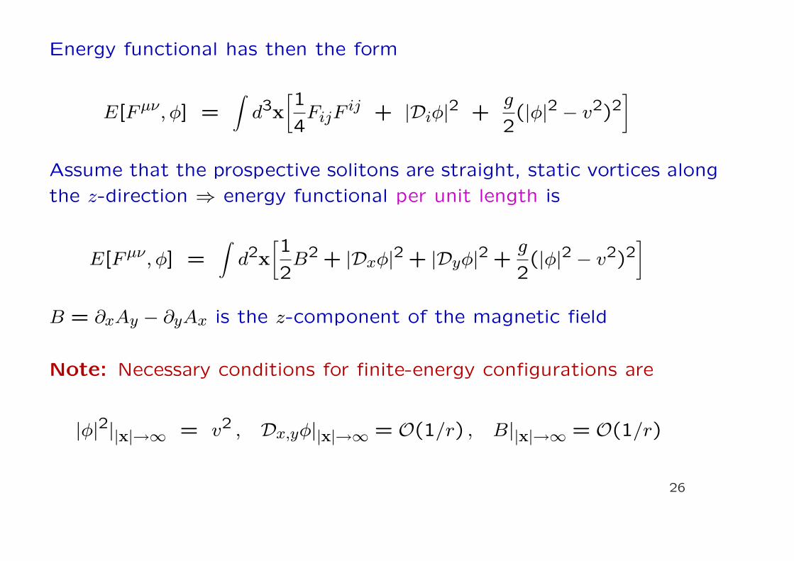
Energy functional has then the form

E[Fµν, φ] =∫

d3x[1

4FijF

ij + |Diφ|2 +g

2(|φ|2 − v2)2

]

Assume that the prospective solitons are straight, static vortices along

the z-direction ⇒ energy functional per unit length is

E[Fµν, φ] =∫

d2x[1

2B2 + |Dxφ|2 + |Dyφ|2 +

g

2(|φ|2 − v2)2

]

B = ∂xAy − ∂yAx is the z-component of the magnetic field

Note: Necessary conditions for finite-energy configurations are

|φ|2||x|→∞ = v2 , Dx,yφ||x|→∞ = O(1/r) , B||x|→∞ = O(1/r)

26

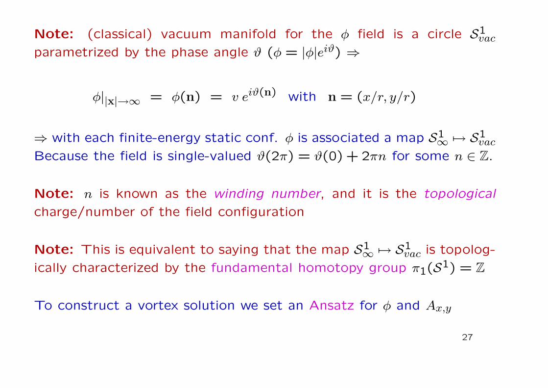
Note: (classical) vacuum manifold for the φ field is a circle S1vac

parametrized by the phase angle ϑ (φ = |φ|eiϑ) ⇒

φ||x|→∞ = φ(n) = v eiϑ(n) with n = (x/r, y/r)

⇒ with each finite-energy static conf. φ is associated a map S1∞ 7→ S1vac

Because the field is single-valued ϑ(2π) = ϑ(0) + 2πn for some n ∈ Z.

Note: n is known as the winding number, and it is the topological

charge/number of the field configuration

Note: This is equivalent to saying that the map S1∞ 7→ S1vac is topolog-

ically characterized by the fundamental homotopy group π1(S1) = Z

To construct a vortex solution we set an Ansatz for φ and Ax,y

27

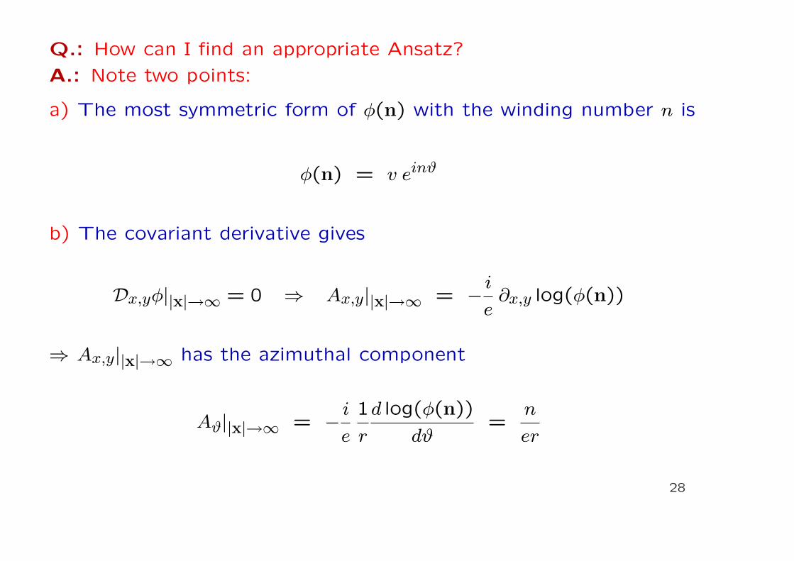
Q.: How can I find an appropriate Ansatz?

A.: Note two points:

a) The most symmetric form of φ(n) with the winding number n is

φ(n) = v einϑ

b) The covariant derivative gives

Dx,yφ||x|→∞ = 0 ⇒ Ax,y||x|→∞ = − i

e∂x,y log(φ(n))

⇒ Ax,y||x|→∞ has the azimuthal component

Aϑ||x|→∞ = − i

e

1

r

d log(φ(n))

dϑ=

n

er

28

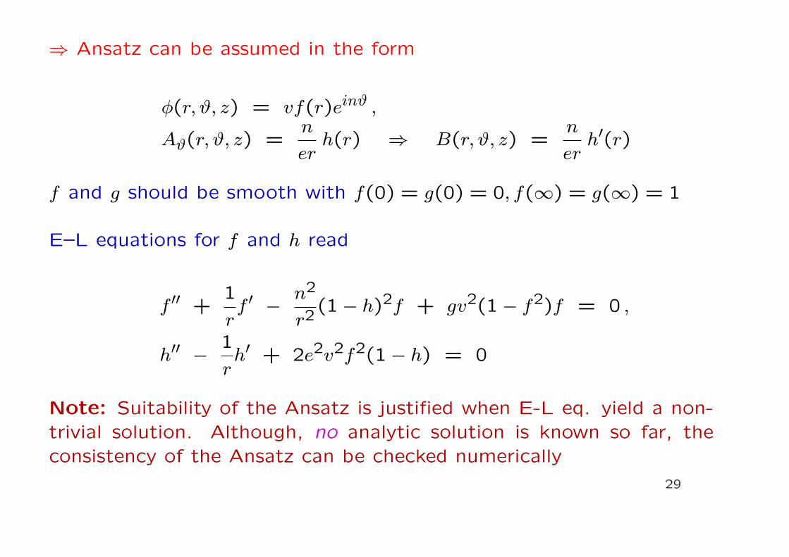
⇒ Ansatz can be assumed in the form

φ(r, ϑ, z) = vf(r)einϑ ,

Aϑ(r, ϑ, z) =n

erh(r) ⇒ B(r, ϑ, z) =

n

erh′(r)

f and g should be smooth with f(0) = g(0) = 0, f(∞) = g(∞) = 1

E–L equations for f and h read

f ′′ +1

rf ′ − n2

r2(1− h)2f + gv2(1− f2)f = 0 ,

h′′ − 1

rh′ + 2e2v2f2(1− h) = 0

Note: Suitability of the Ansatz is justified when E-L eq. yield a non-trivial solution. Although, no analytic solution is known so far, theconsistency of the Ansatz can be checked numerically

29

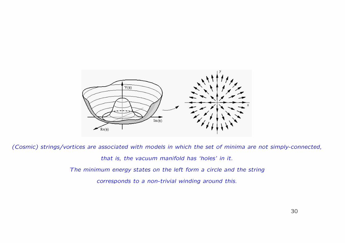
(Cosmic) strings/vortices are associated with models in which the set of minima are not simply-connected,

that is, the vacuum manifold has ‘holes’ in it.

The minimum energy states on the left form a circle and the string

corresponds to a non-trivial winding around this.

30

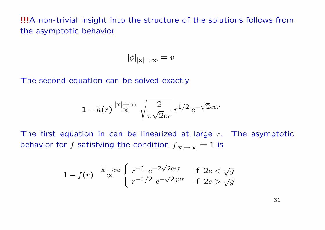
!!!A non-trivial insight into the structure of the solutions follows from

the asymptotic behavior

|φ||x|→∞ = v

The second equation can be solved exactly

1− h(r)|x|→∞∝

√2

π√

2evr1/2 e−

√2evr

The first equation in can be linearized at large r. The asymptotic

behavior for f satisfying the condition f|x|→∞ = 1 is

1− f(r)|x|→∞∝

r−1 e−2√

2evr if 2e <√

g

r−1/2 e−√

2gvr if 2e >√

g

31

Note: There are two length scales governing the large r behavior of f

and h, namely the inverse masses of the scalar and vector excitations

(Higgs and gauge particles), i.e.,

m2s = 2gv2 , m2

v = 2e2v2

Note: Asymptotic behavior depends on the ration (Ginzburg–Landau

parameter)

κ =m2

s

m2v

=g

e2

for κ < 4 the behavior of f is controlled by ms

for κ > 4, mv controls behaviors of f and h

32

Note: In superconductors, the two length scales are known as thecorrelation length ξ = 1/ms and the London penetration depth λ =1/mv

Values of κ distinguish type II and type I superconductors

In type II superconductors ξ < λ

⇒ superconductors can be penetrated by magnetic flux lines

Note: Vortices with |n| > 1 are unstable ⇒ repulsive force betweenparallel n = 1 ⇒ lattice of vortices (Abrikosov vortex lattice)

In type I superconductors ξ > λ

⇒ no penetration by magnetic flux lines (Meissner–Ochsenfeld effect)

33

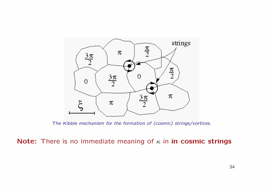
The Kibble mechanism for the formation of (cosmic) strings/vortices.

Note: There is no immediate meaning of κ in in cosmic strings

34

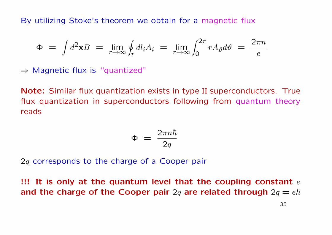
By utilizing Stoke’s theorem we obtain for a magnetic flux

Φ =∫

d2xB = limr→∞

∮

rdliAi = lim

r→∞∫ 2π

0rAϑdϑ =

2πn

e

⇒ Magnetic flux is “quantized”

Note: Similar flux quantization exists in type II superconductors. Trueflux quantization in superconductors following from quantum theoryreads

Φ =2πn~2q

2q corresponds to the charge of a Cooper pair

!!! It is only at the quantum level that the coupling constant e

and the charge of the Cooper pair 2q are related through 2q = e~35

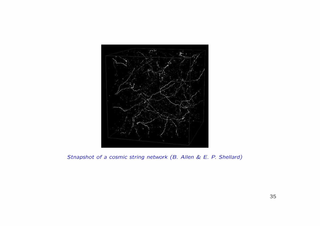
Stnapshot of a cosmic string network (B. Allen & E. P. Shellard)

35

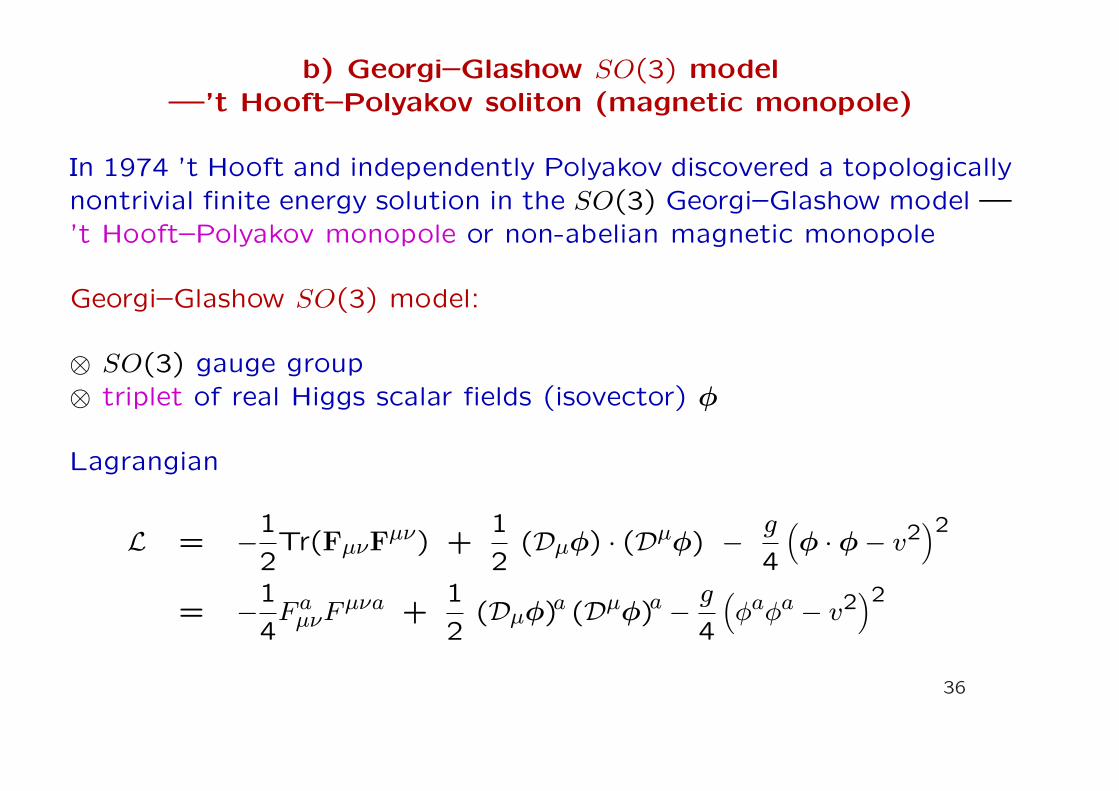
b) Georgi–Glashow SO(3) model—’t Hooft–Polyakov soliton (magnetic monopole)

In 1974 ’t Hooft and independently Polyakov discovered a topologicallynontrivial finite energy solution in the SO(3) Georgi–Glashow model —’t Hooft–Polyakov monopole or non-abelian magnetic monopole

Georgi–Glashow SO(3) model:

⊗ SO(3) gauge group⊗ triplet of real Higgs scalar fields (isovector) φ

Lagrangian

L = −1

2Tr(FµνF

µν) +1

2(Dµφ) · (Dµφ) − g

4

(φ · φ− v2

)2

= −1

4F a

µνFµνa +1

2(Dµφ)a (Dµφ)a − g

4

(φaφa − v2

)2

36

Note: Convention

⊗ µ, ν = 0,1,2,3

⊗ (Killing) normalization for T a s.t. Tr(T aT b) = 12δab

⊗ 3× 3 matrices T a are the SO(3) generators

⊗ Fµν = F aµνT a, Aµ = Aa

µT a

Note: Some elements of non-Abelian gauge theories

Recall that the algebraic structure of d dim. Lie algebra is given by

the commutators

[Ta, Tb] = iC cab Tc

C cab are the structure constants and a = 1, . . . , d

37

Adjoint representation is defined so that

(Ta)c

b = iC cba or equivalently (Ta)bc = −iCabc

⇒ Ta is d× d matrix

Example: adjoint representation for SU(2) ∼= SO(3) has d = 3 ⇒representation space is 3 dim. vector space with matrix elements (Ta)bc:

(Ta)bc = −iεabc

Note: Gauge fields correspond to elements of a Lie algebra in its

adjoint representation

Fundamental representation corresponds to the defining matrix repre-

sentation38

Example:

FR of SO(3) corresponds to 3× 3 orthogonal matrices of determinant1 ⇒ representation space is 3 dim.

FR of SU(2) has 2 dim. representation space

The covariant derivative is

Dµφ = ∂µφ − ieAaµT aφ

e is a real constant (gauge coupling constant)

Under the gauge transformation

φ(x) 7→ g(x)φ(x) ,

Aµ(x) 7→ g(x)Aµ(x)g−1(x) + ie−1(∂µg(x))g−1(x)

39

the covariant derivative transforms covariantly

Dµφ(x) 7→ g(x)Dµφ(x)

The field strength Fµν transforms under the gauge transformation co-

variantly

Fµν = ∂µAν − ∂νAµ + ie[Aµ,Aν] = −ie−1[Dµ,Dν]

7→ gFµνg−1

⇒ L is invariant under the SO(3) gauge group

To show that topological soliton exist in this model we consider static

field configurations with finite energy

40

Static configuration are configurations in the Weyl gauge Aa0 = 0 and

Aai and φa are t indep., i.e.

Aai = Aa

i (x) , φa = φa(x)

⇒ energy functional is

E[Fµν, φ] =∫

d3x[1

4F a

ijFaij +

1

2(Diφ)a (Diφ)a +

g

4

(φaφa − v2

)2]

Necessary condition for the finiteness of the energy is that

(φaφa)||x|→∞ = v2

The vacuum φa may depend on the direction in the physical space, i.e.

φa||x|→∞ = φa(n) n = x/r

41

⇒ each configuration of fields with finite energy is associated with the

mapping S2∞ 7→ S2vac

Note:

From algebraic topology the second homotopy group π2(S2) = Z

⇒ mapping S2∞ 7→ S2vac is classified by integer topological numbers

n = 0,±1,±2, . . .

Q.: How can I choose the soliton Ansatz

A.: Note that the most symmetric form of φa(n) corresponding to a

mapping S2∞ 7→ S2vac is

φa||x|→∞ = nav

As for the asymptotic behavior Aai (x), note the covariant derivative

42

Dµφ = ∂µφ − ieAaµT aφ

must vanish at r →∞. At the same time

∂iφa||x|→∞ =

1

r(δai − nani)v

Requirement of zero covariant derivative → asymptotic gauge field:

Aai (x)||x|→∞ =

1

erεaijnj

Here we have used that (Ta)bc = iεbac and

εijkεilm = δjlδkm − δjmδkl

43

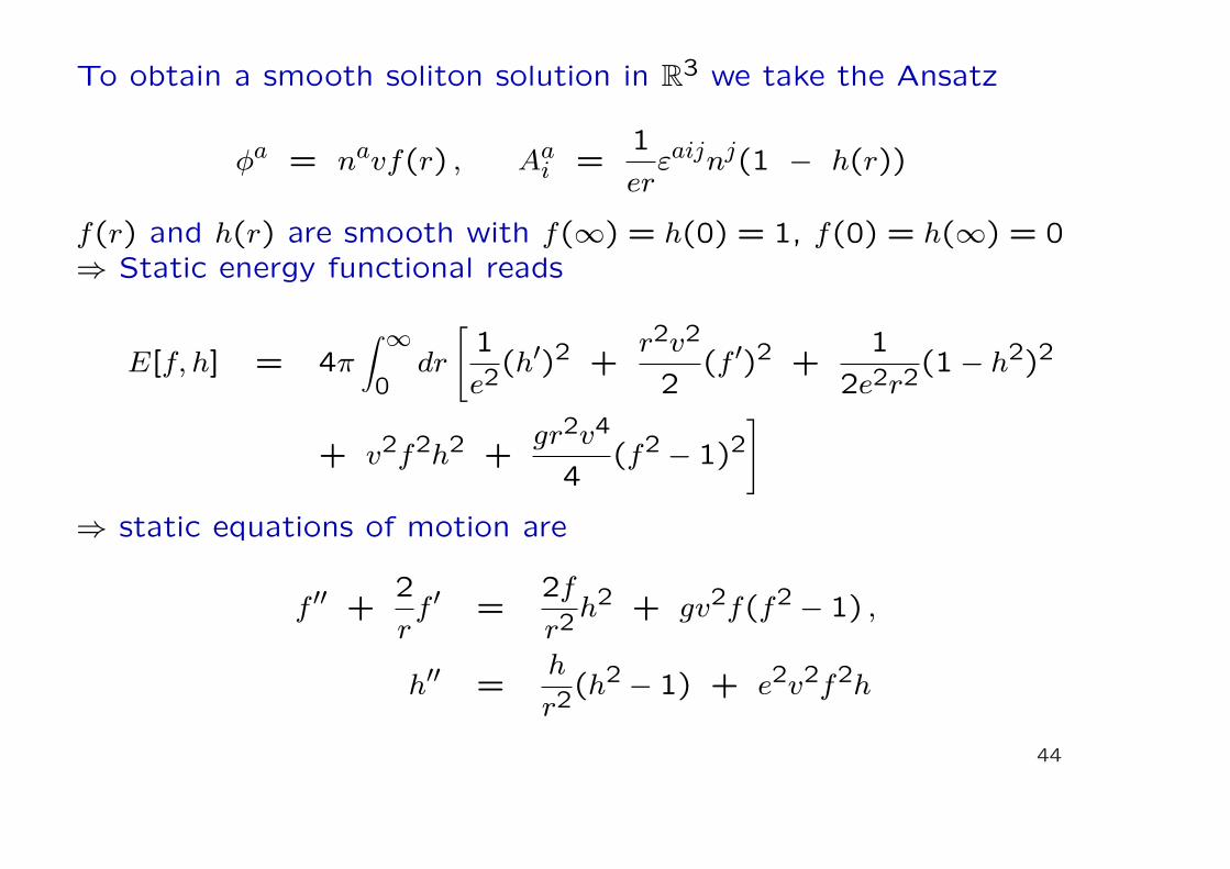
To obtain a smooth soliton solution in R3 we take the Ansatz

φa = navf(r) , Aai =

1

erεaijnj(1 − h(r))

f(r) and h(r) are smooth with f(∞) = h(0) = 1, f(0) = h(∞) = 0⇒ Static energy functional reads

E[f, h] = 4π∫ ∞0

dr

[1

e2(h′)2 +

r2v2

2(f ′)2 +

1

2e2r2(1− h2)2

+ v2f2h2 +gr2v4

4(f2 − 1)2

]

⇒ static equations of motion are

f ′′ +2

rf ′ =

2f

r2h2 + gv2f(f2 − 1) ,

h′′ =h

r2(h2 − 1) + e2v2f2h

44

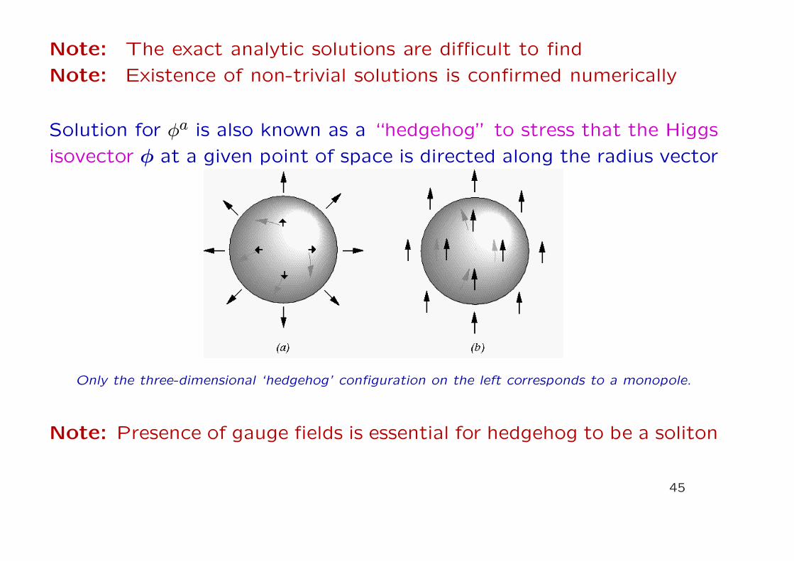
Note: The exact analytic solutions are difficult to find

Note: Existence of non-trivial solutions is confirmed numerically

Solution for φa is also known as a “hedgehog” to stress that the Higgs

isovector φ at a given point of space is directed along the radius vector

Only the three-dimensional ‘hedgehog’ configuration on the left corresponds to a monopole.

Note: Presence of gauge fields is essential for hedgehog to be a soliton

45

Without gauge fields the Higgs field would be linearly divergent corre-

sponding to the infinite rather than finite energy solution

Q.: Why is ’t Hooft–Polyakov soliton a magnetic monopole?

A.: Notice that we have theory with SSB (SO(3) → SO(2)). One

may then identify the unbroken SO(2) ∼= U(1) symmetry with the

electromagnetic field

To be able to identify the (physically observable) electromagnetic field

that is embedded in the original SO(3) theory ’t Hooft proposed the

gauge invariant definition of the electromagnetic field in in the form

Fµν =φa

|v|Faµν − 1

e|v|3εabc φa(Dµφb)(Dνφc)

46

In the broken phase one can chose φa = δ3a|v| then Fµν fulfills the

usual Maxwell equations

Fµν = ∂µA3ν − ∂νA3

µ

⇒ The massless gauge boson corresponding to the unbroken U(1)

group can be identified with the photon i.e., A3µ = Aµ provided we fix

φa = δ3a|v|

⇒ Fµν is a 4× 4 combination of magnetic and electric fields with the

components

Fij = εijkBk, F0i = Ei = 0

⇒ static soliton configuration carries only magnetic field

47

Using that F aµν has at large distances the asymptotic behavior:

F aij

∣∣∣|x|→∞ =nknav

er2εijk =

nk

er2εijk φa||x|→∞ , F a

0i = 0

we have

Bk∣∣∣|x|→∞ =

1

2εkij Fij

∣∣∣|x|→∞ =nk

er2

Applying Gauss’s law, the total magnetic-monopole charge is

Q = limr→∞

∮

S2r

B · ds =4π

e

⇒ ’t Hooft–Polyakov m. satisfies the Dirac-like quantization condition

Qe = 2πn, n ∈ N+

for n = 248

Note: As in the Nielsen–Olesen case, the origin of the “quantization”

condition is purely topological and is not related to the dynamics nor

quantum theory

True Dirac’s quantization condition is Qq = 2π~n (in the CGS units

Qq = ~n/2) Dirac’s quantization condition emerges only at the quan-

tum level which enforces the Lagrange coupling constant e to be related

with the electric charge q via q = ~e

49

Documents

Solitons and instantons in gauge theories - cvut.cz · Solitons and instantons in gauge theories⁄ Petr Jizba FNSPE, Czech Technical University, Prague, Czech Republic ITP, Freie