Embed Size (px)
Citation preview

Solution Manual for Business Statistics 2nd Edition by Donnelly
Link download full: https://testbankservice.com/download/solution-
manual-for-business-statistics-2nd-edition-by-donnelly
CHAPTER 2
Displaying Descriptive Statistics
2.1 a) 2
7 128 100 therefore use 7 classes.
b) 29 512 300 therefore use 9 classes.
c) 210
1, 024 1, 000 therefore use 10 classes.
d) 211
2, 048 2, 000 therefore use 11 classes.
2.2 2 6 64 50 therefore use 6 classes.
Estimated Class Width = 74 −16
= 9.7 10≈ 6
a) 16-25, 26-35, 36-45, 46-55, 56-65, 66-75 b) 16 to under 26, 26 to under 36, 36 to under 46,
46 to under 56, 56 to under 66, 66 to under 76
2.3
Cumulative
Frequency Relative Relative
Number Frequency Frequency
1 6 0.250 0.250
2 6 0.250 0.500
3 5 0.208 0.708
4 4 0.167 0.875
5 3 0.125 1.00
Total 24 1.00
2.4 25 32 30 therefore use 5 classes.
Estimated Class Width = 42.8 −13.9
= 5.8 6 ≈
5

2-1 Copyright ©2015 Pearson Education, Inc.

2-2 Chapter 2
Cumulative
Frequency Relative Relative
Class Frequency Frequency
13 to less than 19 6 0.200 0.200
19 to less than 25 11 0.367 0.567
25 to less than 31 4 0.133 0.700
31 to less than 37 7 0.233 0.933
37 to less than 43 2 0.067 1.0
Total 30 1.00
2.5 2 6 64 36 therefore use 6 classes.
Estimated Class Width = $5, 927 − $162 = $960 $1, 000 ≈
6
a, b, c)
Cumulative
Frequency Relative Relative
Class Frequency Frequency
Less than $1,000 12 0.333 0.333
$1,000 to less than $2,000 8 0.222 0.555
$2,000 to less than $3,000 3 0.083 0.638
$3,000 to less than $4,000 2 0.056 0.694
$4,000 to less than $5,000 6 0.167 0.861
$5,000 to less than $6,000 5 0.139 1.000
Total 36 1.000
d) The following histogram was constructed using bins $999, $1,999, $2,999, $3,999, $4,999,
and $5,999.
Copyright ©2015 Pearson Education, Inc.
Displaying Descriptive Statistics 2-3
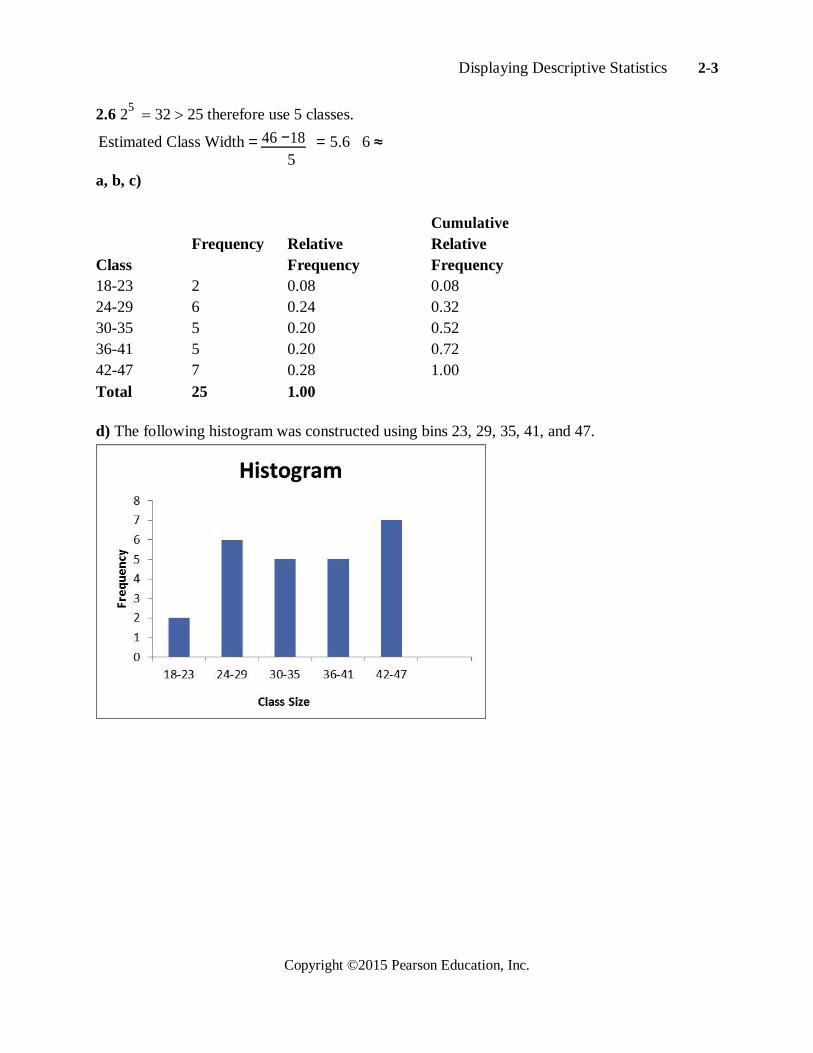
2.6 25 32 25 therefore use 5 classes.
Estimated Class Width = 46 −18 = 5.6 6 ≈
5
a, b, c)
Cumulative
Frequency Relative Relative
Class Frequency Frequency
18-23 2 0.08 0.08
24-29 6 0.24 0.32
30-35 5 0.20 0.52
36-41 5 0.20 0.72
42-47 7 0.28 1.00
Total 25 1.00
d) The following histogram was constructed using bins 23, 29, 35, 41, and 47.
Copyright ©2015 Pearson Education, Inc.

2-4 Chapter 2
2.7
a, b, c)
Cumulative
Frequency Relative Relative
Number Frequency Frequency
0 3 0.043 0.043
1 21 0.300 0.343
2 23 0.329 0.672
3 15 0.214 0.886
4 8 0.114 1.000
Total 70 1.000
d) The following histogram was constructed using bins 0, 1, 2, 3, and 4.
2.8 2 6 64 40 therefore use 6 classes.
Estimated Class Width (Current) = 76 −19
= 9.5 10≈ 6
Results would be similar using the laid-off ages.
Class Bins Midpoint
19 to less than 29 28.9 24
29 to less than 39 38.9 34
39 to less than 49 48.9 44
49 to less than 59 58.9 54
59 to less than 69 68.9 64
69 to less than 79 78.9 74
Copyright ©2015 Pearson Education, Inc.

Displaying Descriptive Statistics 2-5
An extra bin (18.9) was added to Excel to provide the open-ended class required by PHStat.
a)
b)
Copyright ©2015 Pearson Education, Inc.

2-6 Chapter 2
c) According to these polygons, it appears that the current workforce is younger than the laid-off
employees. It appears that the laid-off employees may have a case for age discrimination.
2.9 29 512 350 therefore use 9 classes.
Estimated Class Width = $349.99 − $2.19
= $38.64 $40 ≈ 9
a, b, c)
Cumulative
Frequency Relative Relative
Class Frequency Frequency
Less than $40 52 0.149 0.149
$40 to less than $80 103 0.294 0.443
$80 to less than $120 91 0.260 0.703
$120 to less than $160 65 0.186 0.889
$160 to less than $200 15 0.043 0.932
$200 to less than $240 11 0.031 0.963
$240 to less than $280 5 0.014 0.977
$280 to less than $320 5 0.014 0.991
$320 to less than $360 3 0.009 1.000
Total 350 1.000
d) The following histogram was constructed using bins 39.999, 79.999, 119.999, 159.999,
199.999, 239.999, 279.999, 319.999, and 359.999.
Copyright ©2015 Pearson Education, Inc.

Displaying Descriptive Statistics 2-7
2.10 2 7 128 125 therefore use 7 classes.
Estimated Class Width = 83.2 − 71.0
= 1.7 2 ≈
7
a, b, c)
Cumulative
Frequency Relative Relative
Class Frequency Frequency
71 to less than 73 5 0.040 0.040
73 to less than 75 37 0.296 0.336
75 to less than 77 44 0.352 0.688
77 to less than 79 31 0.248 0.936
79 to less than 81 6 0.048 0.984
81 to less than 83 1 0.008 0.992
83 to less than 85 1 0.008 1.000
Total 125 1.000
d) The following histogram was constructed using bins 72.99, 74.99, 76.99, 78.99, 80.99, 82.99,
and 84.99.
e) For 68.8% of the days, ocean temps were lower than 77 degrees.
Copyright ©2015 Pearson Education, Inc.

2-8 Chapter 2
2.11
a, b, c)
Cumulative
Frequency Relative Relative
Category Frequency Frequency
Google 20 0.667 0.667
Yahoo 5 0.167 0.833
Bing 2 0.067 0.900
Baidu 2 0.067 0.967
Other 1 0.033 1.000
Total 30 1.000
d)
2.12
a, b, c)
Cumulative
Frequency Relative Relative
Category Frequency Frequency
Excellent 16 0.267 0.267
Good 31 0.517 0.783
Fair 8 0.133 0.917
Poor 5 0.083 1.000
Total 60 1.000
Copyright ©2015 Pearson Education, Inc.

Displaying Descriptive Statistics 2-9
d)
e) 78.3% rated their dining experience as either Excellent or Good.
2.13
Copyright ©2015 Pearson Education, Inc.

2-10 Chapter 2
2.14
2.15
Copyright ©2015 Pearson Education, Inc.

Displaying Descriptive Statistics 2-11
2.16
2.17
2.18
Copyright ©2015 Pearson Education, Inc.

2-12 Chapter 2
2.19 Because all the possible categories appear to be included in the data, a pie chart would be
a good choice to display this data.
2.20 Because we are comparing data from a sample of countries over different time periods, a
clustered bar chart would be a good choice to display this data. A stacked bar chart would not be
the best choice because adding the GDPs for 2 time periods that are 10 years apart is not very
meaningful.
2.21
Grade Female Male Total
A 5 2 7
B 5 7 12
C 2 3 5
Total 12 12 24
Copyright ©2015 Pearson Education, Inc.
Displaying Descriptive Statistics 2-13
71% (5/7) of the As were earned by females even though they comprise of 50% (12/24) of the
students in the class. The females appear to have done better grade-wise than the males.
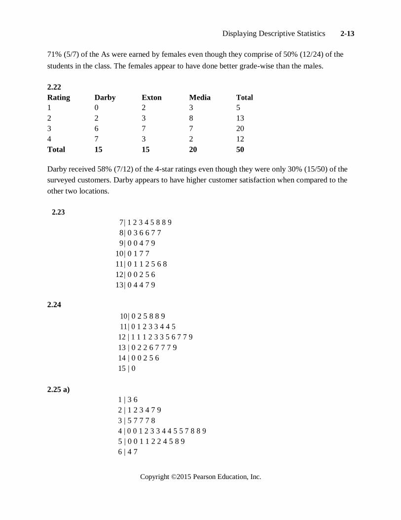
2.22
Rating Darby Exton Media Total
1 0 2 3 5
2 2 3 8 13
3 6 7 7 20
4 7 3 2 12
Total 15 15 20 50
Darby received 58% (7/12) of the 4-star ratings even though they were only 30% (15/50) of the
surveyed customers. Darby appears to have higher customer satisfaction when compared to the
other two locations.
2.23
7 | 1 2 3 4 5 8 8 9
8 | 0 3 6 6 7 7
9 | 0 0 4 7 9
10 | 0 1 7 7
11 | 0 1 1 2 5 6 8
12 | 0 0 2 5 6
13 | 0 4 4 7 9
2.24
10 | 0 2 5 8 8 9
11 | 0 1 2 3 3 4 4 5
12 | 1 1 1 2 3 3 5 6 7 7 9
13 | 0 2 2 6 7 7 7 9
14 | 0 0 2 5 6
15 | 0
2.25 a)
1 | 3 6
2 | 1 2 3 4 7 9
3 | 5 7 7 7 8
4 | 0 0 1 2 3 3 4 4 5 5 7 8 8 9
5 | 0 0 1 1 2 2 4 5 8 9
6 | 4 7
Copyright ©2015 Pearson Education, Inc.
2-14 Chapter 2
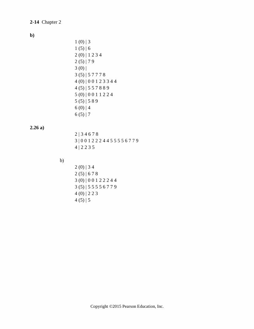
b)
1 (0) | 3
1 (5) | 6
2 (0) | 1 2 3 4
2 (5) | 7 9
3 (0) |
3 (5) | 5 7 7 7 8
4 (0) | 0 0 1 2 3 3 4 4
4 (5) | 5 5 7 8 8 9
5 (0) | 0 0 1 1 2 2 4
5 (5) | 5 8 9
6 (0) | 4
6 (5) | 7
2.26 a)
2 | 3 4 6 7 8
3 | 0 0 1 2 2 2 4 4 5 5 5 5 6 7 7 9
4 | 2 2 3 5
b)
2 (0) | 3 4
2 (5) | 6 7 8
3 (0) | 0 0 1 2 2 2 4 4
3 (5) | 5 5 5 5 6 7 7 9
4 (0) | 2 2 3
4 (5) | 5
Copyright ©2015 Pearson Education, Inc.

Displaying Descriptive Statistics 2-15
2.27 It appears that the number of Netflix subscribers is increasing during this time period.
2.28 There does not appear to be a consistent relationship between the amount of time on the
web site and the order size.
Copyright ©2015 Pearson Education, Inc.

2-16 Chapter 2
2.29
2.30 2 6 64 40 therefore use 6 classes.
Estimated Class Width = 23 − 0 = 3.8 4≈
6
a, b, c)
Cumulative
Frequency Relative Relative
Class Frequency Frequency
0-3 8 0.200 0.200
4-7 5 0.125 0.325
8-11 15 0.375 0.700
12-15 3 0.075 0.775
16-19 6 0.150 0.925
20-23 3 0.075 1.000
Total 40 1.000
d) The following histogram was constructed using bins 3, 7, 11, 15, 19, and 23.
Copyright ©2015 Pearson Education, Inc.

Displaying Descriptive Statistics 2-17
2.31
a, b, c)
Cumulative
Frequency Relative Relative
Number Frequency Frequency
0 16 0.32 0.32
1 9 0.18 0.50
2 7 0.14 0.64
3 11 0.22 0.86
4 5 0.10 0.96
5 2 0.04 1.00
Total 50 1.00 d) The following histogram was constructed using bins 0, 1, 2, 3, 4, and 5.
Copyright ©2015 Pearson Education, Inc.

2-18 Chapter 2
e) 50%
2.32 2 6 64 48 therefore use 6 classes.
Estimated Class Width = 1,187 − 43
= 190.7 200≈
6
a, b, c)
Cumulative
Frequency Relative Relative
Class Frequency Frequency
0 to under 200 15 0.313 0.313
200 to under 400 13 0.271 0.584
400 to under 600 11 0.229 0.813
600 to under 800 4 0.083 0.896
800 to under 1,000 4 0.083 0.979
1,000 to under 1,200 1 0.021 1.000
Total 48 1.000
d) The following histogram was constructed using bins 199.9, 399.9, 599.9, 799.9, 999.9,
and 1,199.9.
2.33 2 7 128 72 therefore use 7 classes.
Estimated Class Width = 795 −190
= 86.4 100≈ 7
Copyright ©2015 Pearson Education, Inc.

Displaying Descriptive Statistics 2-19
a, b, c)
Cumulative
Frequency Relative Relative
Class Frequency Frequency
101-200 2 0.028 0.028
201-300 2 0.028 0.056
301-400 9 0.125 0.181
401-500 15 0.208 0.389
501-600 31 0.431 0.820
601-700 9 0.125 0.945
701-800 4 0.056 1.001
Total 72 1.001
d) The following histogram was constructed using bins 200, 300, 400, 500, 600, 700, and 800.
2.34 25 32 30 therefore use 5 classes.
Estimated Class Width (Day) = 100 − 66
= 6.8 7 ≈ 5
Results would be similar using the evening grades.
Class Bins Midpoint
66-72 72 69
73-79 79 76
80-86 86 83
87-93 93 90
94-100 100 97
Copyright ©2015 Pearson Education, Inc.

2-20 Chapter 2
An extra bin (65) was added to Excel to provide the open-ended class required by PHStat.
a)
b)
c) The evening class grades appear to be noticeably higher than the day class grades.
Copyright ©2015 Pearson Education, Inc.

Displaying Descriptive Statistics 2-21
2.35 29 512 300 therefore use 9 classes.
Estimated Class Width = 39 − −14
= 5.9 6 ≈ 9
a, b, c)
Relative
Frequency Relative Cumulative
Class Frequency Frequency
–14 to under –8 6 0.020 0.020
–8 to under –2 28 0.093 0.113
–2 to under 4 40 0.133 0.246
4 to under 10 58 0.193 0.439
10 to under 16 68 0.227 0.666
16 to under 22 61 0.203 0.869
22 to under 28 27 0.090 0.959
28 to under 34 9 0.030 0.989
34 to under 40 3 0.010 0.999
Total 300 0.999
d) The following histogram was constructed using bins –8.1, –2.1, 3.9, 9.9, 15.9, 21.9, 27.9, 33.9, and 39.9.
e) Approximately 226 out of 300 flights were not late (75.3%).
Copyright ©2015 Pearson Education, Inc.

2-22 Chapter 2
2.36 a)
b)
2.37 2 7 128 100 therefore use 7 classes.
Estimated Class Width (Wayne) = 259 −12 = 35.3 40≈
7
Results would be similar using the Dover data.
Class Bins Midpoint
1-40 40 20.5
41-80 80 60.5
81-120 120 100.5
121-160 160 140.5
161-200 200 180.5
201-240 240 220.5
241-280 280 260.5
An extra bin (0) was added to Excel to provide the open-ended class required by PHStat.
Copyright ©2015 Pearson Education, Inc.
Displaying Descriptive Statistics 2-23
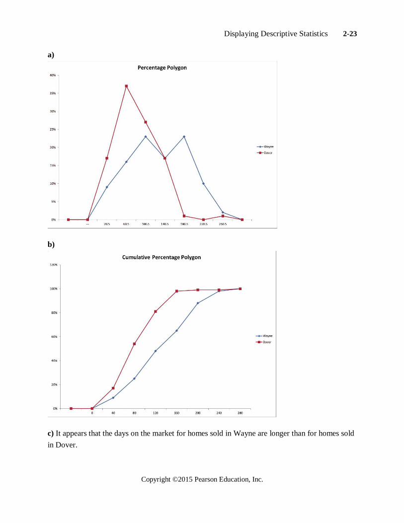
a)
b)
c) It appears that the days on the market for homes sold in Wayne are longer than for homes sold
in Dover.
Copyright ©2015 Pearson Education, Inc.

2-24 Chapter 2
2.38 a)
b)
Copyright ©2015 Pearson Education, Inc.
Displaying Descriptive Statistics 2-25
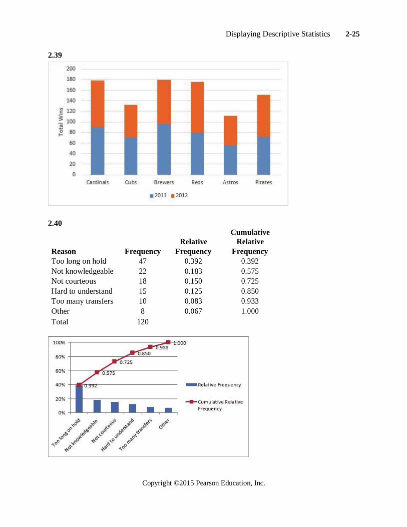
2.39
2.40
Cumulative
Relative Relative
Reason Frequency Frequency Frequency
Too long on hold 47 0.392 0.392
Not knowledgeable 22 0.183 0.575
Not courteous 18 0.150 0.725
Hard to understand 15 0.125 0.850
Too many transfers 10 0.083 0.933
Other 8 0.067 1.000
Total 120
Copyright ©2015 Pearson Education, Inc.

2-26 Chapter 2
2.41
Relative Cumulative
Reason Frequency Frequency Relative Frequency
Transmission 721 0.385 0.385
Body 437 0.233 0.619
Wheels 164 0.088 0.706
Drivetrain 139 0.074 0.780
Windows 89 0.048 0.828
Engine 55 0.029 0.857
Interior 45 0.024 0.881
Electrical 44 0.024 0.905
Steering 42 0.022 0.927
Suspension 41 0.022 0.949
AC/heater 26 0.014 0.963
Brakes 22 0.012 0.975
Other 47 0.025 1.000
Total 1872
Copyright ©2015 Pearson Education, Inc.

Displaying Descriptive Statistics 2-27
2.42
2.43
Copyright ©2015 Pearson Education, Inc.

2-28 Chapter 2
2.44
2.45 A bar chart would be appropriate for categorical data. The time data needs to be converted
to common units (minutes).
Copyright ©2015 Pearson Education, Inc.

Displaying Descriptive Statistics 2-29
2.46 A clustered bar chart would be appropriate for this data. A stacked bar chart would also
be an option.
2.47 A bar chart, either horizontal or vertical, is the best choice for this data. A pie chart would
not be appropriate because all brands are not included. The total percentage does not equal
100%.
Copyright ©2015 Pearson Education, Inc.

2-30 Chapter 2
2.48 A pie chart is the best choice because all categories are included and the percentage sums to 100%.
2.49 A bar chart, either horizontal or vertical, is the best choice for this data.
Copyright ©2015 Pearson Education, Inc.

Displaying Descriptive Statistics 2-31
2.50 A bar chart is the best display for qualitative data organized in categories.
2.51 A bar chart is the best display for quantitative data organized in categories.
Copyright ©2015 Pearson Education, Inc.

2-32 Chapter 2
2.52 Pie charts are a good choice for displaying qualitative data when the proportions add to 100%.
2.53 A stacked bar chart is the best choice to compare totals from different groups.
2.54 26 64 55 therefore use 6 classes.
Estimated Class Width = 66 − 26
= 6.7 7 ≈ 6
Copyright ©2015 Pearson Education, Inc.

Displaying Descriptive Statistics 2-33
a, b, c)
Cumulative
Frequency Relative Relative
Class Frequency Frequency
26-32 11 0.200 0.200
33-39 10 0.182 0.382
40-46 16 0.291 0.673
47-53 12 0.218 0.891
54-60 4 0.073 0.964
61-67 2 0.036 1.00
Total 55 1.00
d) The following histogram was constructed using bins 32, 39, 46, 53, 60 and 67.
Copyright ©2015 Pearson Education, Inc.

2-34 Chapter 2
2.55 A pie chart is the best choice because the probabilities add to 100%.
2.56 a, b, c)
Cumulative
Frequency Relative Relative
Class Frequency Frequency
0 2 0.033 0.033
1 1 0.017 0.050
2 13 0.217 0.267
3 16 0.267 0.554
4 11 0.183 0.717
5 10 0.167 0.884
6 4 0.067 0.951
7 3 0.050 1.001
Total 60 1.001
Copyright ©2015 Pearson Education, Inc.

Displaying Descriptive Statistics 2-35
d) The following histogram was constructed using bins 0, 1, 2, 3, 4, 5, 6 and 7.
2.57 a)
6 | 4 7 7 9 9
7 | 0 0 0 1 1 1 4 5 6 7 7 8
8 | 1 2 3 5 6 7 7 8 9
9 | 0 0 1 5 6 7 8
10 | 2 4
11 | 7
b)
6 (0) | 4
6 (5) | 7 7 9 9
7 (0) | 0 0 0 1 1 1 4
7 (5) | 5 6 7 7 8
8 (0) | 1 2 3
8 (5) | 5 6 7 7 8 9
9 (0) | 0 0 1
9 (5) | 5 6 7 8
10 (0) | 2 4
10 (5) |
11 (0) |
11 (5) | 7
Copyright ©2015 Pearson Education, Inc.
2-36 Chapter 2
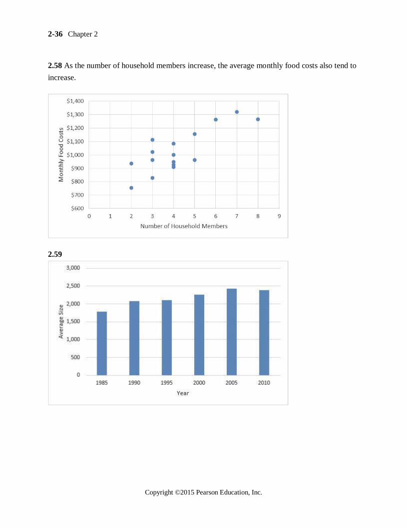
2.58 As the number of household members increase, the average monthly food costs also tend to
increase.
2.59
Copyright ©2015 Pearson Education, Inc.

Displaying Descriptive Statistics 2-37
2.60
2.61
a, b, c)
Cumulative
Frequency Relative Relative
Category Frequency Frequency
Cheez-Its 16 0.667 0.667
Cheese Nips 5 0.208 0.875
No Prefer 3 0.125 1.000
Total 24 1.000
2.62
1 | 2 3 5 8
2 | 1 1 3 6 6 7 7 8
3 | 0 3 3 5 6 6 9
4 | 0 0 2 2 4 6 7 9
5 | 0 1 7
Copyright ©2015 Pearson Education, Inc.

2-38 Chapter 2
2.63
2.64
Brand Diet Regular Total
Coke 6 6 12
Mt. Dew 2 8 10
Pepsi 4 7 11
Total 12 21 33
50% (6/12) of the Coke customers preferred Diet even though only 36% (12/33) of all the
customers prefer Diet soda. Coke customers appear to have a higher percentage of
customers who prefer diet soda than other brands.
2.65
Age Callaway Nike Taylor Made Total
20-29 4 2 19 25
30-39 9 15 10 34
40-49 16 6 8 30
50-59 3 3 5 11
Total 32 26 42 100
Younger golfers seem to prefer Taylor Made clubs while older golfers seem to refer Callaway.
Copyright ©2015 Pearson Education, Inc.

Displaying Descriptive Statistics 2-39
2.66 a) 1 | 8 9 9
2 | 0 0 0 2 2 3 3 5 5 5 6 8 8 8 8 9 3 | 0 1 1 1 1 2 2 3 5 5 5 6 6 9 9
4 | 1 3 3 5 6
5 | 1
b)
1 (5) | 8 9 9
2 (0) | 0 0 0 2 2 3 3
2 (5) | 5 5 5 6 8 8 8 8 9
3 (0) | 0 1 1 1 1 2 2 3
3 (5) | 5 5 5 6 6 9 9
4 (0) | 1 3 3
4 (5) | 5 6
5 (0) | 1
2.67 a) 7 | 0 0 2 2 4 5 6 7 7 7
8 | 1 2 5 8 9 | 0 1 2 2 3 3 3 4 5 7 7 9 9
10 | 0 1 2 4 5
11 | 2 8 9
12 | 5
13 | 0 0 1 8
Copyright ©2015 Pearson Education, Inc.

2-40 Chapter 2
b)
7 (0) | 0 0 2 2 4
7 (5) | 5 6 7 7 7
8 (0) | 1 2
8 (5) | 5 8
9 (0) | 0 1 2 2 3 3 3 4
9 (5) | 5 7 7 9 9
10 (0) | 0 1 2 4
10 (5) | 5
11 (0) | 2
11 (5) | 8 9
12 (0) |
12 (5) | 5
13 (0) | 0 0 1
13 (5) | 8
2.68
There does not appear to be a consistent relationship between payroll and wins during the 2012
season.
Copyright ©2015 Pearson Education, Inc.

Displaying Descriptive Statistics 2-41
2.69
The trend in gasoline prices appear to rise consistently except for the time period around Month
220.
2.70
a)
Status
Airline Late On Time Total
Delta 5 38 43
Southwest 5 22 27
United 7 23 30
Total 17 83 100
b)
Status
Airline Late On Time Total
Delta 0.05 0.38 0.43
Southwest 0.05 0.22 0.27
United 0.07 0.23 0.30
Total 0.17 0.83 1.00
c) Delta has the highest on-time percentage (38/43 = 0.88) while United has the lowest (23/30
= 0.77)
Copyright ©2015 Pearson Education, Inc.

2-42 Chapter 2
2.71
Using Chicago data, 2 6 64 60 therefore use 6 classes.
Estimated Class Width = 85 −1
= 14.0 ≈15 6
Class Bins Midpoint
0 to less than 15 14.9 7.5
15 to less than 30 29.9 22.5
30 to less than 45 44.9 37.5
45 to less than 60 59.9 52.5
60 to less than 75 74.9 67.5
75 to less than 90 89.9 82.5
An extra bin (–0.1) was added to Excel to provide the open-ended class required by PHStat.
Copyright ©2015 Pearson Education, Inc.

Displaying Descriptive Statistics 2-43
2.72 A line chart would be the best display for these data.
Copyright ©2015 Pearson Education, Inc.