Solution of discrete-time optimal control problems on ...pages.cs.wisc.edu/~swright/papers/WrightParallelComputing90.pdf · Solution of discrete-time optimal control problems on parallel

Parallel Comput ing 16 (1990) 221-237 221 North-Holland

Solution of discrete-time optimal control problems on parallel computers *

Stephen J. W R I G H T

Department of Mathematics, Box 8205, North Carolina State University, Raleigh, NC27695, USA

Received August 1989 Revised J anua ry / June 1990

Abstract. We describe locally-convergent algorithms for discrete-time optimal control problems which are amenable to multiprocessor implementation. Parallelism is achieved both through concurrent evaluation of the component functions and their derivatives, and through the use of a parallel band solver which solves a linear system to find the step at each iteration. Results from an implementation on the Alliant F X / 8 are described.

Keywords. Discrete-time optimal control problems, Constrained optimization problem, Parallel band solver, Multiprocessor implementation, Shared memory multiprocessor.

1. Introduction

The uncons t ra ined N-stage d iscre te- t ime op t ima l cont ro l p r o b l e m with Bolza object ives has the form

N def N + 1

m i n F ( u ) = IN+I(X ) + Y'. l , ( x i, U') (1.1) u i=1

x t = a (f ixed) (1.2)

X i + l = f i ( x i ' u i ) ,

where x i ~ R n, i = 1 . . . . . N + 1, and u i ~ R m, i = 1 . . . . . N. The x i var iables are usual ly referred to as states and the u i as controls. This p r o b l e m m a y arise, for example as a d iscre t iza t ion of the con t inuous- t ime p r o b l e m

minflL(x(t), u(t), t )dt + u(t) J0

s . t . ~ = f ( x , u, t), x ( 0 ) = x 0 ,

(Polak [12], J acobson and M a y n e [7], Kel ley and Sachs [8]), bu t it is also of in teres t in its own right in model l ing cer ta in phys ica l processes.

In some s i tuat ions there may be stagewise cons t ra in ts on the x ~ and u~; in their mos t general form these can be wri t ten as

g i ( x i , u i) <.~ O, i = 1 . . . . . N , (1.3)

* Research partially performed while the author was visiting Argonne National Laboratory, Argonne, IL, and supported by the National Science Foundat ion under Grants DMS-8619903, DMS-8900984 and ASC-8714009, and the Air Force Office of Scientific Research under Grant AFOSR-ISSA-87-0092

0167-8191/90/$03.50 © 1990 - Elsevier Science Publishers B.V. (North-Holland)

222 SJ. Wright / Discrete-time optimal control problems

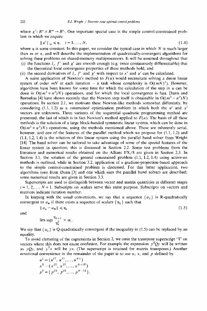
where gi: R" × R m ~ R ~'. One important special case is the simple control-constrained problem in which we require

II u ' l l~ ~<n, i = 1 . . . . . N, (1.4)

where 77 is some constant. In this paper, we consider the typical case in which N is much larger than m or n, and will describe the implementation of quadratically-convergent algorithms for solving these problems on shared-memory multiprocessors. It will be assumed throughout that (i) the functions l i, f f and gi are smooth enough (e.g. twice continuously differentiable) that

the theoretical local convergence properties of these methods hold, and (ii) the second derivatives of l~, f~ and g~ with respect to x ~ and u ~ can be calculated.

A naive application of Newton's method to F(u) would necessitate solving a dense linear system of order mN at each iteration - a task whose complexity is O((mN)3). However, algorithms have been known for some time for which the calculation of the step in u can be done in O((m3 + n3)N) operations, and for which the local convergence is fast. Dunn and Bertsekas [4] have shown recently that the Newton step itself is obtainable in O((m 3 + n3)N) operations. In section 2.1, we motivate these Newton-like methods somewhat differently, by considering (1.1, 1.2) as a constrained optimization problem in which both the u ~ and x i vectors are unknowns. Three variants of the sequential quadratic programming method are presented, the last of which is in fact Newton's method applied to F(u). The basis of all these methods is the solution of a large block-banded symmetric linear system, which can be done in O((m3 + n3)N) operations, using the methods mentioned above. These are inherently serial, however, and one of the features of the parallel method which we propose for (1.1, 1.2) and (1.1, 1.2, 1.4) is the solution of this linear system using the parallel band solver from Wright [14]. The band solver can be tailored to take advantage of some of the special features of the linear system in question; this is discussed in Section 2.2. Some test problems from the literature and numerical results obtained on the Alliant F X / 8 are given in Section 2.3. In Section 3.1, the solution of the general constrained problem (1.1, 1.2, 1.4) using active-set methods is outlined, while in Section 3.2, application of a gradient-projection-based approach to the simple control-constrained problem is discussed. For this latter application, two algorithms (one from Dunn [3] and one which uses the parallel band solver) are described; some numerical results are given in Section 3.3.

Superscripts are used to distinguish between vector and matrix quantities at different stages i = 1, 2 . . . . . N + 1. Subscripts on scalars serve this same purpose. Subscripts on vectors and matrices indicate iteration number.

In keeping with the usual conventions, we say that a sequence {a k } is R-quadratically convergent to a , if there exists a sequence of scalars { ~/k } such that

II a k - - a , II ~ nk (1.5) and

T/k+1 lim sup ~ < ~ .

We say that { a k } is Q-quadratically convergent if the inequality in (1.5) can be replaced by an equality.

To avoid cluttering of the expressions in Section 2, we omit the transpose superscript 'T ' on vectors where this does not cause confusion. For example the expression yTQy will be written as yQy, and y~x will be yx. (The superscript is retained for matrix transposes.) Another notational convenience in the remainder of the paper is to use u, x, and p defined by

( u < u . . . . . u

xT= (X 2T, x3T,..., X N+IT) pX= (p2-r, p3"r . . . . . pN+IT).

S.J. Wright / Discrete-time optimal control problems 223

(p*+~ is the Lagrange multiplier vector for the 'constraint' (1.2).) In keeping with omission of

the transpose on vectors, (u, x, p) will be used for .

2. The unconstrained problem

2.1 Algorithms with fast local convergence

Specialized algorithms for solving (1.1) which are both quadratically convergent and for which the cost of calculating successive iterates increases only linearly with N have been known for some time. The best-known examples are the differential dynamic programming (DDP) algorithm of Jacobson and Mayne [7] and the method described by Polak [12, pp. 92-102]. The DDP algorithm is quadratically convergent in u, since it produces steps which are asymptotically similar to Newton steps. It was used in preference to Newton's method because it was apparently believed for some time that the Newton step is much more expensive to calculate. This is not true; Dunn and Bertsekas [4] show that the Newton step can be obtained by using dynamic programming to solve a linear-quadratic optimal control problem. Polak's approach also solves a linear-quadratic subproblem.

In this section, we consider the treatment of (1.1, 1.2) as a problem in constrained optimization, where x and u are both variable and the state equations (1.2) are constraints. Application of the sequential quadratic programming (SQP) method yields, under the usual second-order sufficiency assumptions, Q-quadratic convergence in the triple (u, x, p), where the vector p is made up of Lagrange multipliers pi+l which correspond to the 'constraint' x i+ 1 = f i(xi ' u i). Modifications to the SQP algorithm produce variants which are Q-quadratically convergent in (u, x) and in u alone; the latter is in fact Newton's method. These variants are successively less parallelizable, and since there is little practical difference in the convergence rates (all are R-quadratically convergent in u), SQP should certainly be considered as an alternative to Newton's method, at least in the neighbourhood of a solution. We take up this point later.

We assume throughout that there are vectors u, and x , which satisfy second-order sufficient conditions to be a solution of (1.1). These are defined after we have introduced some notation. Further, we assume that all iterates are sufficiently close to u, and x , that the usual local convergence properties hold. Convergence to a solution from an arbitrary starting point is of course desirable from a practical point of view - a Levenberg-style modification is discussed in Dunn and Bertsekas [4] which would help in this aim. We put this issue aside here, since we are mainly concerned with the basic algorithm and its implementation in a parallel setting.

The Lagrangian for (1.1) is, using the notation already introduced for Lagrange multipliers, N N

~L#(u, x , p ) = IN+I(X N+I) + E li( xi , ui) -- E ( x i + l - f i ( xi , u i ) ) P i+1 (2.1) i~1 i = l

First-order conditions for (u, x, p) to be a solution of (1.1) are that

~,~ al i i a f i+l 3u ~ ~u i + ~ u ~ p = 0 , i = l . . . . . N (2.2)

i a£~' ~l i pi + 3 f i+1 3x ~ 3x ~ ~ x , p = 0 , i = 2 . . . . . N (2.3)

~"~ ~IN+I pN+l 3xN+ 1 ~xN+ 1 = 0 (2.4)

~L/:' x *+' + f i ( x i , u ~) = O, i = 1 . . . . . N . (2.5) ~pi+l

224 S.J. Wright / Discrete-time optimal control problems

(Here we have fixed X 1 = a and eliminated it from the problem.) We introduce the following notation, some of which has been used elsewhere (Dunn [3], Dunn and Bertsekas [4]), although defined there in terms of Hamiltonians rather than the Lagrangian.

Qi = " Ri = - - ; s i = O(ui.)2 ' ~(x i ) 2 ' ~x i abl i

a i = Of i . B i = Of i . t i = O S r i = ~¢~ Ox i ' Ou ~ , Ox i , Ou i •

(2.6)

Assumption 1. There exist vectors u. and x . which satisfy second-order sufficient conditions for (1.1), that is,

(i) there exists at least one vector p . such that the equations (2.2-2.5) hold (with all quantities evaluated at (u. , x.)),

(ii) for some p . satisfying (i), and all nonzero directions (v, y) such that

yl = 0

yi+l = A , , y i + Bi .v i

we have that

that is,

(v, y)W2Lf(u, , x , , p , ) ( v , y ) > 0 ,

N 1 N + I ~ N + I N + I " " " 7Y ~ . Y + ½ Y'. ( Y ' Q ' . Y ' + 2 y i R i . v i + vSi*v ' ) > 0

i=l

(where the subscript ' , ' denotes evaluation at (u, , x , , p,)).

It is well known (see Fletcher [5]) that in the neighbourhood of a point (u. , x .) satisfying Assumption 1, SQP is equivalent to applying Newton's method to (2.2-2.5). In the following, we use v i, y i and qi to denote components of the Newton steps in the control, state and multiplier vectors (Su, 8x and 8p) respectively. Linearization of (2.2-2.5) gives the following system to be solved to find these quantities:

r i + RiTy i + Sly i + BiTq i+l = 0,

t i + Riv i + Qiyi _ qi +AiTqi+l = O,

i N + l + Q N + l y N + I _ qN+I = 0 ,

[__xi+l + f i ( x i ' ui)] __yi+l + Aiyi + B i d = O ,

Using the notation

pi= Oil ~i Oli y = __xi+l + f i ( x i ' Hi), O U i ' O X i '

(2.7-2.10) can be written alternatively as

pi + RiTyi + Sivi + BiXp++l = O,

~i + R i d + Oiy i _ p + + AiTp++l= 0,

?N+I + QN+lyN+1 _pN++l = 0,

~i __ yi+ l + Aiyi + Biv i = O,

i = 1 . . . . , N, (2.7)

i = 1 . . . . . N, (2.8)

(2.9)

i = 1 . . . . . N. (2.10)

p + = p + q ,

i = 1 . . . . . N, (2.11)

i = 2 . . . . . N , (2.12)

(2.13)

i = 1 . . . . . N . (2.14)


The (locally equivalent) SQP form of (2.7-2.10) is of course N

lnln E rivi + tiy i+ l ( y i p i y i + 2ytRivi + vtSiv i) _~_ tN+lyN+a _}_ lyN+IQN+lyN+I v,y i=1

yl =0

(2.15)

s . t . y i+1 = A i y i w B i v i + ~ i, i = l , . . . , N .

where the q~ are the Lagrange multipliers for the (linear) constraints at the solution of (2.15). The system (2.11-2.14) has a similar quadratic-programming representation, with the optimal Lagrange multipliers being p++ 1 instead of qi+ 1

We can summarize the resulting algorithm as follows:

Algorithm I (SQP/Lagrange-Newton).

k~-O repeat

1. Solve (2.7-2.10) (or the alternatives) for v i, yi and qi+l (or p,++l) 2. Set

u i ~ u i + v i, i = 1 , . . . , N

x i~ - - - x i+y i, i = 2 . . . . , N + 1

p i+ l ,__p i+ l+q i+ l=p++l , i = l , . . . , N

3. k * - - k + 1 until convergence.

The following convergence result is a standard one for SQP methods; its proof is omitted.

Theorem 2.1. Let u , and x , satisfy the second-order sufficient conditions for (1.1) with optimal Lag, range multipliers p , . Denote the sequence of iterates produced by Algorithm I as ( uk, Xk, Pk )" Then if the initial estimates (Uo, Xo, Po) are sufficiently close to (u , , x , , p , ) , the estimate

II(Uk+a - - U , , X k + ~ - - X , , Pk+l --P*)II = o ( II(Uk -- u , , X k - - X,, Pk --P*)II 2)

holds, that is, the sequence ( ( Uk, Xk, Pk) ) is Q-quadratically convergent.

One variant of this approach is to update the multipliers pi+l using the formulae (2.3-2.4), rather than setting pi+l ~ p%÷ 1. The resulting algorithm is

Algorithm II.

k~-O repeat

1. Solve (2.7-2.10) (or the alternatives) for v i, yi and qi+l (or p++l) 2. Set

ui"c----ui-3t-v i, i = 1 . . . . , N

xi ~'-- xi'q- y i, i = 2 , . . . , N + l

3. Evaluate A i, F, i = 2 . . . . . N (at the new (u, x ) iterate) 4. p N + l * - - t N + l ; f o r i = N . . . . ,2 pi~--ti+AiTpi+l; 5. k ~ k + l

until convergence.


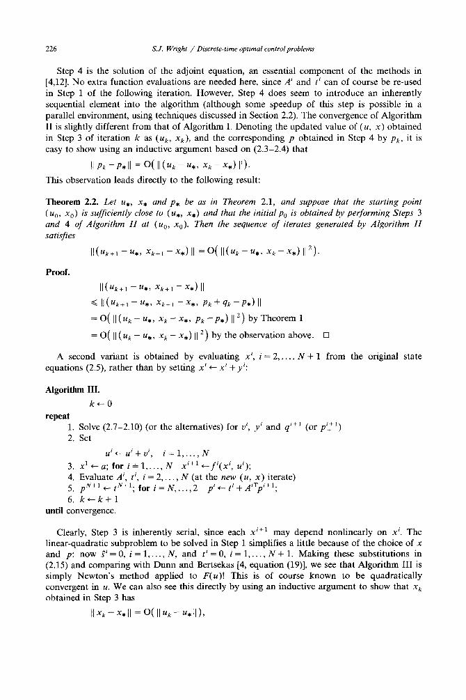
Step 4 is the solution of the adjoint equation, an essential component of the methods in [4,12]. No extra function evaluations are needed here, since A ~ and t ~ can of course be re-used in Step 1 of the following iteration. However, Step 4 does seem to introduce an inherently sequential element into the algorithm (although some speedup of this step is possible in a parallel environment, using techniques discussed in Section 2.2). The convergence of Algorithm II is slightly different from that of Algorithm I. Denoting the updated value of (u, x) obtained in Step 3 of iteration k as (u k, xk), and the corresponding p obtained in Step 4 by Pk, it is easy to show using an inductive argument based on (2.3-2.4) that

II p k - p , II = o ( II ( u k - u , , xk - x , ) II) .

This observation leads directly to the following result:

Theorem 2.2. Let u,, x , and p , be as in Theorem 2.1, and suppose that the starting point ( Uo, xo) is sufficiently close to ( u,, x , ) and that the initial po is obtained by performing Steps 3 and 4 of Algorithm H at (Uo, Xo). Then the sequence of iterates generated by Algorithm H satisfies

II(Uk+l--U., Xk+I--X.)II = O ( [ l ( U k - U . , Xk - -X . ) 112).

Proof.

I I ( u k + l - u , , x ~ + l - x , ) I I

~< II ( u k ÷ l - u , , x k ÷ l - x , , Pk + qk - P * ) II

= O ( II ( u k - u , , xk - x , , p k - P , ) I I 2) by T h e o r e m 1

= O( I[(u~ - u , , xk - x , ) I I 2) by the observation above. []

A second variant is obtained by evaluating x i, i = 2 . . . . . N + 1 from the original state equations (2.5), rather than by setting x i ~ x~+ y~:

Algorithm III.

k , - 0 repeat

1. Solve (2.7-2.10) (or the alternatives) for v i, yi and qi+l (or p/+÷l) 2. Set

u ~ u i + v ~, i = l , . . . , N 3. x 1 ~ a; for i = 1 . . . . . N X i+l ~"-fi(xi, ui); 4. Evaluate A i, t i, i = 2 . . . . . N (at the new (u, x ) iterate) 5. pS+l ~ t u + l ; for i = N , . . . , 2 pi~'-ti-I-AiTpi+l; 6. k ~ k + l

until convergence.

Clearly, Step 3 is inherently serial, since each M +1 may depend nonlinearly on x i. The linear-quadratic subproblem to be solved in Step 1 simplifies a little because of the choice of x and p; now g~ = 0, i = 1 . . . . . N, and t i = 0, i = 1 . . . . . N + 1. Making these substitutions in (2.15) and comparing with Dunn and Bertsekas [4, equation (19)], we see that Algorithm III is simply Newton's method applied to F(u)! This is of course known to be quadratically convergent in u. We can also see this directly by using an inductive argument to show that x k obtained in Step 3 has

II xk - x , II = O ( II u~ - u , II) ,


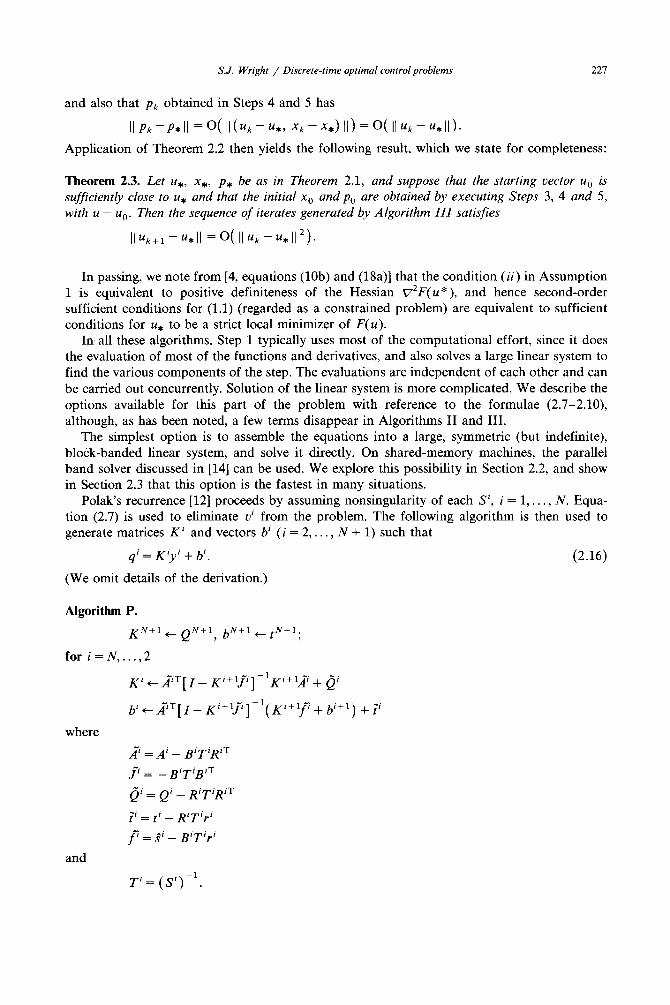
and also that Pk obtained in Steps 4 and 5 has

II pk - p , II = O ( I I (uk - u , , xk - x , ) II) = O ( II uk - u , II).

Application of Theorem 2.2 then yields the following result, which we state for completeness:

Theorem 2.3. Let u,, x , , p , be as in Theorem 2.1, and suppose that the starting vector u o is sufficiently close to u , and that the initial x o and Po are obtained by executing Steps 3, 4 and 5, with u = u o. Then the sequence of iterates generated by Algorithm I I I satisfies

II Uk-I-1 - - U , II = O ( II uk - u , II 2) .

In passing, we note from [4, equations (10b) and (18a)] that the condition ( i i) in Assumption 1 is equivalent to positive definiteness of the Hessian V'EF(u *), and hence second-order sufficient conditions for (1.1) (regarded as a constrained problem) are equivalent to sufficient conditions for u, to be a strict local minimizer of F(u) .

In all these algorithms, Step 1 typically uses most of the computational effort, since it does the evaluation of most of the functions and derivatives, and also solves a large linear system to find the various components of the step. The evaluations are independent of each other and can be carried out concurrently. Solution of the linear system is more complicated. We describe the options available for this part of the problem with reference to the formulae (2.7-2.10), although, as has been noted, a few terms disappear in Algorithms II and III.

The simplest option is to assemble the equations into a large, symmetric (but indefinite), block-banded linear system, and solve it directly. On shared-memory machines, the parallel band solver discussed in [14] can be used. We explore this possibility in Section 2.2, and show in Section 2.3 that this option is the fastest in many situations.

Polak's recurrence [12] proceeds by assuming nonsingularity of each S ~, i = 1 . . . . . N. Equa- tion (2.7) is used to eliminate v ~ from the problem. The following algorithm is then used to generate matrices K i and vectors b ~ (i = 2 . . . . . N + 1) such that

qi = K i y i + b i. (2.16)

(We omit details of the derivation.)

Algorithm

for i = N , .

where

and

P°

K N + I ~ QN+I , bN+l ~._tN+l;

. . , 2

K i , - - 2 T [ I - K ' + a f ] - IK~+I~ + ~

b' ~__ ~ T [ I _ K i + l f i ] - l ( K i + l f i + bi+l) + ?i

.~i = A i _ B i T t R i T

f i = _ B i T , B i T

O i = Qi _ R i T t R i T

,{i = t i _ R i T i r i

f i = gi -- B i Z i r i

T'= (S')


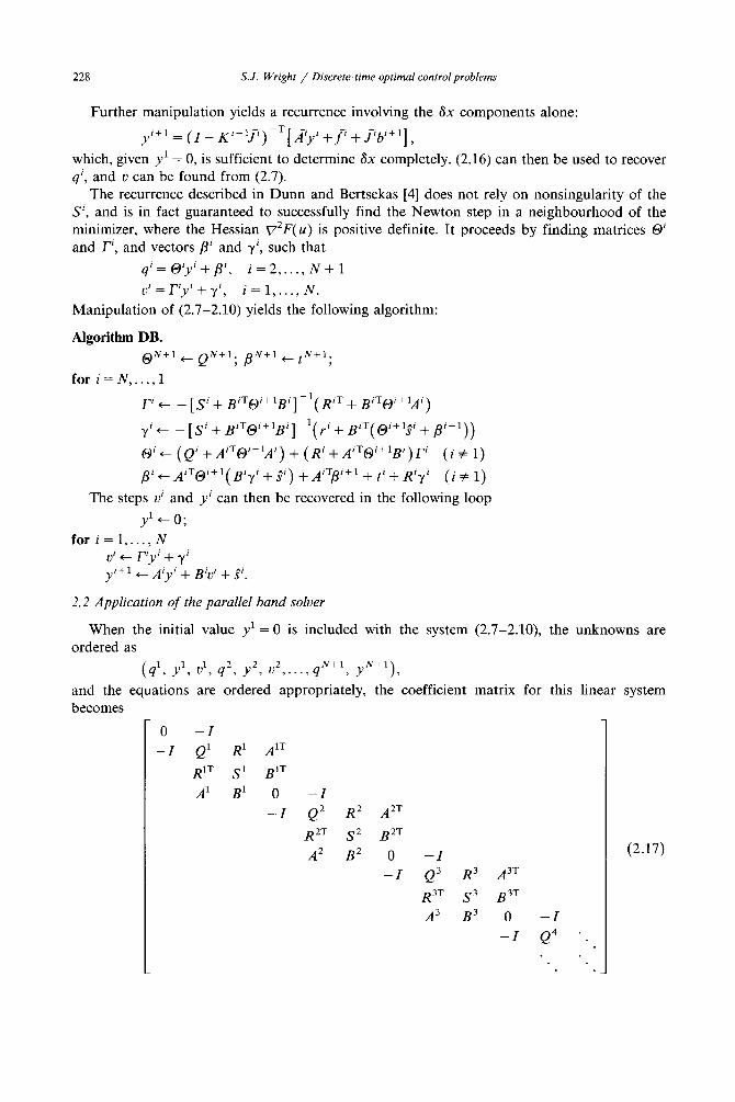
Further manipulation yields a recurrence involving the 6x components alone:

yi+l = ( I - K i + l f i) -T[.,4iy i + f f + f ibi+l] ,

which, given yl = 0, is sufficient to determine 3x completely. (2.16) can then be used to recover qi, and v can be found from (2.7).

The recurrence described in Dunn and Bertsekas [4] does not rely on nonsingularity of the S i, and is in fact guaranteed to successfully find the Newton step in a neighbourhood of the minimizer, where the Hessian ~72F(u) is positive definite. It proceeds by finding matrices O' and F i, and vectors fli and 7 ~, such that

q i=O~y ~+fl~, i = 2 . . . . . N + I # = Fiyi + 7i , i = l , . . . , N.

Manipulation of (2.7-2.10) yields the following algorithm:

A l g o r i t h m D B .

~N+I <___ QN+I; ~N+I 4._ tN+l;

f o r i = N . . . . . 1

Ci ~.._ _ [ s i n t- BiT[~i+IB i ] - I (RiT _}_ BiToi+ IA i)

vi,__ _ [ s i + BiTOi+,Bi ] ' ( r i + BiT({~i+l~i q_ ]~i+1))

0 i~-- (Qiq-AiTOi+lAi) q- (Riq-AiTOi+lBi)Ci (i=# 1)

fli ,__ AiTOi+l( Biy, + gi) +A,Tfli+I + t ' + Riv ' (i * 1)

The steps # and y~ can then be recovered in the following loop yl ~-- 0;

f o r i = 1 . . . . . N Vi ~ Fiyi 4_ .~i yi+l ~__Aiyi q_Bivi.k_~i"

2.2 Application of the parallel band solver

When the initial value y l = 0 is included with the system (2.7-2.10), the unknowns are ordered as

(ql, 71, 01, q2, y2, V2 . . . . . qN+l, TN+I),

ordered appropriately, the coefficient matrix for this linear system and the equations are becomes

0 - I - I Q1

R iT A 1

R 1 A 1T

S 1 B 1T

B 1 0

- I

- I Q2 R2 A2T

R 2T S 2 B 2T

A 2 9 2 0

- I - I Q3 R3 A3T

R 3T S 3 B 3T

A 3 B 3 0

- I

- I Q4

(2.17)


with a right-hand side of

( 0 , - - t 1 , - - r 1 , - =+t, _ t 2 , _ r 2 , _ g2 . . . . . _ g N , _ t N + , ) . ( 2 . 1 8 )

This matrix is symmetric, with dimension 2 n ( N + 1) + raN, and a half-bandwidth of (2n + m - 1). In the neighbourhood of a solution which satisfies Assumption 1, it will be nonsingular.

We now give a brief description in general terms of the algorithm, described in [14], for solving banded linear systems on a P-processor shared-memory multiprocessor. Suppose the system to be solved is

F x = c, F ~ R M×M,

where F has half-bandwidth k, that is F,j = 0 when l i - j I > k. We assume impicitly that M is large and k is by comparison very small. The method starts by dissecting F along its diagonal into P large blocks, with each pair of large blocks separated by a smaller k × k block. Notat ion for the blocks 9roduced by the dissection is introduced by writing F as:

F 1 C 12

T 12 D 1 T 21

C 21 F 2

T 22

F =

C 22

D 2 T 31

C 3l F 3 C 32

T P - 1,2 D e - 1 TP,1

C el F p

Here the main blocks F j are square, with half-bandwidth k, and have approximately equal dimensions M e , where M e = M / P - k. The separator blocks D j are k × k and dense, while the left and right flanking matrices C j'l and C J'2 are Mp × k, and the top and bot tom flanking matrices T j'l and T j'2 are k × M e. A symmetric row and column dissection reordering is applied to F, giving

F 1 C 12

F 2 C 21 C 22

FP-1 C p 1,1 cP-1,2

P A F H A = F p C pl

T 12 T 21 D 1

T 22 T 31 D 2

T p - I,2 Tpl D p - 1

Each block F j is then assigned to a single processor, where it is factorized using an 'enhanced row pivoting' strategy, to give

p / F i n J = L(2 ) I J[ 0 V a J

where L j and U j are square, and lower and upper triangular respectively, while the blocks I and V J are square with dimension at most 2k. If F j is well-conditioned, it is usually the case that i i i = I and that the usual row-partial-pivoting factorization P J F J = L J U j is obtained.


However, because of the partitioning above, the F j may be ill-conditioned or even singular (with rank at least M e - 2k), so column pivoting may also be needed for stability.

The U j factors are also used to eliminate the blocks T j'~ and T J'2 which now appear in the bot tom left of the reordered system, giving rise to multiplier matrices M j ' l and M j'2 in the overall L factor of F. In addition, more symmetric row and column pivoting is performed on the overall matrix to move the U(~) and V j blocks out of the top left partition. At this point, we have produced a partial L U factorization

P B F H B = L U ,

where

Z =

L ~ L 2

L~2)

U=

U 1

L P

U 2

M P - 1,2 M P 1

U p

I

~ 2

0

I

~ - 1,2

C 1

0 P The Schur complement ff contains fill-in which is generated during the elimination of the

T j'~ and T j'2 blocks, and during the row and column reordering which takes place after factorization of the individual blocks. The remainder of the algorithm consists of factorizing ff on a single processor, and then recovering the solution using back- and forward-substitution. For further information the reader is referred to [14].

A slightly modified version of this algorithm is used to solve (2.17-2.18). Each separator block D j is chosen to be

D j = R i T S i T ,

A i B i B~ 0

for some value of i. The dimension of D j is (2n + m), rather than the (2n + m - 1) which would follow from the direct application of the general bandsolver. However, the blocks C j'a, C j'2, T j'a and T j'2 induced by this choice of D j contain a number of zero rows and columns, which give rise to computational savings during the factorization process. The total amount of fill-in will be smaller, and the reduced system will have a narrower bandwidth than in the general case.


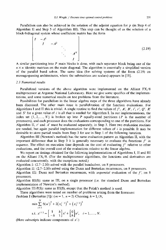
Parallelism can also be achieved in the solution of the adjoint equation for p (in Step 4 of Algorithm II and Step 5 of Algorithm III). This step can be thought of as the solution of a block-bidia ~onal system whose coefficient matrix has the form

- I --A 1 I - A 2

(2.19) _ A N

I

A similar partitioning into P main blocks is done, with each separator block being one of the n x n identity matrices on the main diagonal. The algorithm is essentially a simplified version of the parallel band solver. The same idea (for solving systems of the form (2.19) on message-passing architectures, where the submatrices are scalars) appears in [11].

2.3 Numerical results

Parallelized versions of the above algorithm were implemented on the Alliant F X / 8 multiprocessor at Argonne National Laboratory. Here we give some specifics of the implementations, and some numerical results on test problems from the literature.

Possibilities for parallelism in the linear algebra steps of the three algorithms have already been discussed. The other main issue is parallelization of the function evaluations. For Algorithms | and II this is trivial. A single routine to find the values of f i , A i, B i, t i, r i, Qi, R i and S ~ for a given value of i is all that is needed for Algorithm I. In our implementations, the index set {1, 2 . . . . . N ) is broken up into P equally-sized partitions (P is the number of processors), and each processor does the evaluations corresponding to one of the partitions. For Algorithm II, t ~ and A i must be evaluated separately, in Step 3. Here two evaluation routines are needed, but again parallel implementation for different values of i is possible. It may be desirable to store partial results from Step 3 for use in Step 1 of the following iteration.

Algorithm III (Newton's method) has the same evaluation pattern as Algorithm II, with the important difference that in Step 3 it is generally necessary to evaluate the functions f~ in sequence. The effect on execution time depends on the cost of evaluating f i relative to other evaluations, and the overall cost of the evaluations relative to the linear algebra.

We report on timings obtained for the following implementations of Algorithms I, II and III on the Alliant FX/8 . (For the multiprocessor algorithms, the functions and derivatives are evaluated concurrently, with the exceptions noted.) Algorithm I: (2.7-2.10) solved with the parallel bandsolver, on 8 processors. Algorithm II: (2.7-2.10) solved using the Dunn and Bertsekas recurrences, on 8 processors. Algorithm III: Dunn and Bertsekas recurrences, with sequential evaluation of the f~, on 8 processors. Algorithm III(S): same as III, on a single processor (i.e. the standard Dunn and Bertsekas implementation of Newton's method). Algorithm III-P(S): same as III(S), except that the Polak's method is used.

These algorithms were tested on number of problems arising from the literature: Problem I (Bertsekas [1]): (rn = 1, n = 2) Choosing h = 1/N,

N rain E 5(ui) 2+ 2(x~+l) 2+ (xi+l) 2

i = l

0 i

(Here subscripts indicate components of M.)


Problem 2 (Kelley and Sachs [8]): (m = 1, n = 1) This problem is a discretization of the continuous problem

f0 , 4 ( / ) rain °30 .5e- ' ( (x ( t ) - l.5)2 + ( u ( t ) - 3)2) + ~ dt u(t)

s.t. 2 ( t ) = u ( t ) - t 2, x(O)=l.

Given a value of N, set h = 0.3/N and look for u i to approximate u( ( i - 0.5)h) and x i to approximate x ( ( i - 1)h). The integral can be replaced by a trapezoidal rule, and the state equation by the midpoint rule approximation

X i + l = X i --~ hu i - h 3 ( i - 0 . 5 ) 2.

Problem 3 (Di Pillo, Grippo and Lampariello [2]): (m = 1, n = 2) In the terminology of (1.1, 1.2), and choosing h = 1/N,

l,(x,, . , )= + + (.,)2]

f i (x ' , u i )

+ 5hx

Problem 2A: (m = 1, n = 1) This is the same as Problem 2, except that each function and derivative evaluation is done 100 times. Hence the computation time is (artificially) dominated by evaluations rather than by the linear algebra•

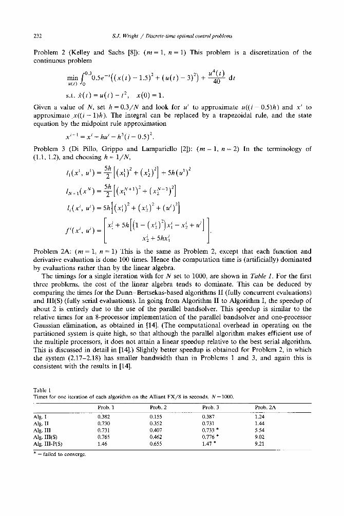
The timings for a single iteration with for N set to 1000, are shown in Table 1. For the first three problems, the cost of the linear algebra tends to dominate. This can be deduced by comparing the times for the Dunn-Bertsekas-based algorithms II (fully concurrent evaluations) and III(S) (fully serial evaluations). In going from Algorithm II to Algorithm I, the speedup of about 2 is entirely due to the use of the parallel bandsolver. This speedup is similar to the relative times for an 8-processor implementation of the parallel bandsolver and one-processor Gaussian elimination, as obtained in [14]. (The computational overhead in operating on the partitioned system is quite high, so that although the parallel algorithm makes efficient use of the multiple processors, it does not attain a linear speedup relative to the best serial algorithm. This is discussed in detail in [14]•) Slightly better speedup is obtained for Problem 2, in which the system (2•17-2.18) has smaller bandwidth than in Problems 1 and 3, and again this is consistent with the results in [14]•

Table 1 Times for one iteration of each algorithm on the Alliant F X / 8 in seconds, N = 1000.

Prob. 1 Prob. 2 Prob. 3 Prob. 2A

Alg. I 0.382 0.155 0.387 1.24 Alg. II 0.730 0.352 0.731 1.44 Alg. III 0.731 0.407 0.733 * 5.54 Alg. Ill(S) 0.765 0.462 0.776 * 9.02 Alg. III-P(S) 1.46 0.655 1.47 * 9.21

* = failed to converge.


In Problem 2A, the function evaluations dominate the computation, and we see a progressive improvement in going from the serial algorithm III(S), to the 'partially parallel' III, to the 'fully parallel' II. The advantage gained by using the parallel band solver (Algorithm I) is smaller in a relative sense than in the other problems. However, it is clear by comparing Algorithm I with Algorithm III(S) that a highly efficient 8-processor implementation has been achieved.

Im summary, on an 8-processor machine, we can obtain an algorithm which is two to three times faster than the best serial implementation of Newton's method, for problems in which the linear algebra dominates, and almost eight times faster than Newton's method, when the function evaluations dominate.

We stress again that only the 'no-frills' locally convergent algorithms have been implemented above. For practical codes, it will be necessary to include features which ensure global convergence. Also, it may be desirable to make use of the chord method, in which the second-derivative matrices are not calculated (and factorized) on every iteration.

3. The constrained problem

3.1 Active set methods

Inclusion of the general constraints (1.3) gives a more difficult problem, which can again be solved in a sequential quadratic programming framework. We sketch the approach in this section. There are two variants of SQP for handling inequality constraints, known in the literature as ' IQP' and 'EQP'. In IQP, the constraints (1.3) are linearized at each step, and the quadratic subproblem (2.15) is solved subject to the additional constraints

gi(xi, u i ) + f ~-~gi(xi, ui)+oi~---ffgi(xi, ui)<..O, i = 1 . . . . . N. (3.1)

The other terms r i, t i, Qi, R i, and S ~ in (2.15) need to be redefined in terms of a Lagrangian with an additional term:

N N ~QP(Id, X, p, ~) = IN+I(X N+I) "[- E l i (x" U') -- E ( X/+I - - f i ( X`' U/))P/+1

i=1 i=1 N

+ E g'(x', i=l

The quadratic programming problem (2.15, 3.1) can be solved using an active set approach, where at each minor iteration a subset of the components of (3.1) are chosen to hold at equality, and the remainder are ignored, at least until a line search is done. Hence (2.15) may be repeatedly solved subject to constraints of the form

gS(x', u') + y' gS(x', u') + v' -u gS(x', (3.2) j ~ a i c {1 . . . . . v~}, i = 1 . . . . . N.

Writing down the first order conditions for this subproblem, we obtain a set of linear equations in d, y~, qi, and /~) ( j ~ A~) which is obtained by augmenting (2.7-2.10) with appropriate terms in /~i, and including the equations (3.2). Again these equations can be solved via recurrence relations (see Ohno [9], or Dunn [3] and Pantoja and Mayne [10] for the case in which the gi are functions of u ~ only). Alternatively, after an appropriate ordering of equations and variables, a block-banded system is again obtained, which can again be solved with the parallel band solver.


In the EQP approach, the active constraint sets A i are fixed during each outer iteration, rather than at each minor iteration as in IQP. The innermost iteration is identical in form to that of IQP, namely (2.15, 3~2), and hence can be solved as before. The relative merits of IQP and EQP have been extensively discussed elsewhere (see for example Powell [13]).

We do not pursue these approaches further here, since they are often unsuitable for large-scale problems. The reason for this is that the active set A = (A1 . . . . . A N ) is generally only allowed to change by a small number of components at each (major or minor) iteration. Hence if the initial estimate of A is far from the optimal active set, many iterations will be required.

Once the correct active constraint manifold has been identified, these algorithms are R-quadratically convergent in u.

3.2 The simple control-constrained case - a gradient projection method

An alternative to active set methods, which is attractive when the feasible region defined by the constraints (1.3) is convex and has simple geometry, is the two-metric gradient projection algorithm (see Bertsekas [1], Gafni and Bertsekas [6] and Dunn [3]). This method has the advantage that large changes to the active set are allowed at each iteration, while it retains the good local convergence properties of the active set algorithms.

We sketch this approach for the important special case in which the constraints have the form (1.4) (see Bertsekas [1] for the details). The problem (1.1, 1.2) is regarded as a function of u alone (i.e. F(u)). As in Algorithm III of Section 2, x is obtained from the state equations (1.2) and p is obtained from the adjoint equation (2.3), so that in (2.15), t i = 0 and gi = 0. At each iteration, an 'almost-active set' A = {A1 . . . . . AN} is constructed, where Ai contains the indices of the components of u ~ which at or near their bound +7 , and for which the corresponding component of ~TF(u) has the "correct" sign (i.e. 3F/~u~ > 0 if u ~ -- j - ~/ and

i 3F/Ouj < 0 if Ug = 7)- (2.15) is then solved, using the definitions of Q', R ', S i and r ' from (2.1) and (2.6), subject to the additional constraints

v j = 0 , j~-A~, i = l . . . . . N. (3.3)

This process yields the 'Newton ' part of the step. The 'first-order ' part can be obtained by setting

v j= o ~ F - JOu----7' J ~ A i , i = 1 . . . . . N

i (where _o ~< Og ~< #, _o and 6 being positive constants; we choose oj = 1). A search is then carried out along the piecewise-linear path P(u + av), a ~ [0, 1], where P denotes projection of a vector in R km onto the box (w ~ Rkmlwi ~ [-~/, ~/]). An Armijo linesearch strategy is used, that is, the values a = 1, fl, f12 . . . . (13 < 1) are tried, until a sufficient decrease criterion is met. For this value of a, u is reset to P(u + av) for the next iteration. The values of x and p are recalculated accordingly.

Solution of the constrained problem (2.15, 3.3) can be done using a modified version of the recurrences in Algorithm DB (see Dunn [3]), which we state below. Let Pi be the matrix

e T pi=[ j ] j ~ . ,

where ej is the j t h column of the m × m identity matrix. Also for any m × m matrix S, denote pispiT by [S]ii.

Algorithm DB(C) o N + I = Q N + I ; ~ N + I = t N + l ;

s.J. Wright / Discrete-time optimal control problems 235

f o r i = N , . . . , 1

F ' ~ - [ S ' + BiTo'+ 'Bi],-~ aP'( R 'T + BiT(gi+ IA i)

.yi .._ _ [ S i + BiT(gi+lBi]i~lpi(r i + BiT((gi+l~i + /~i+1))

(9' ~ (Q ' + AiToi+IA i) + ( R i + A ' T o ' + I B ' ) p ' T F ' (i # 1)

' + + A'TB '+ ' + t ' + R'e'T ' ( i . 1)

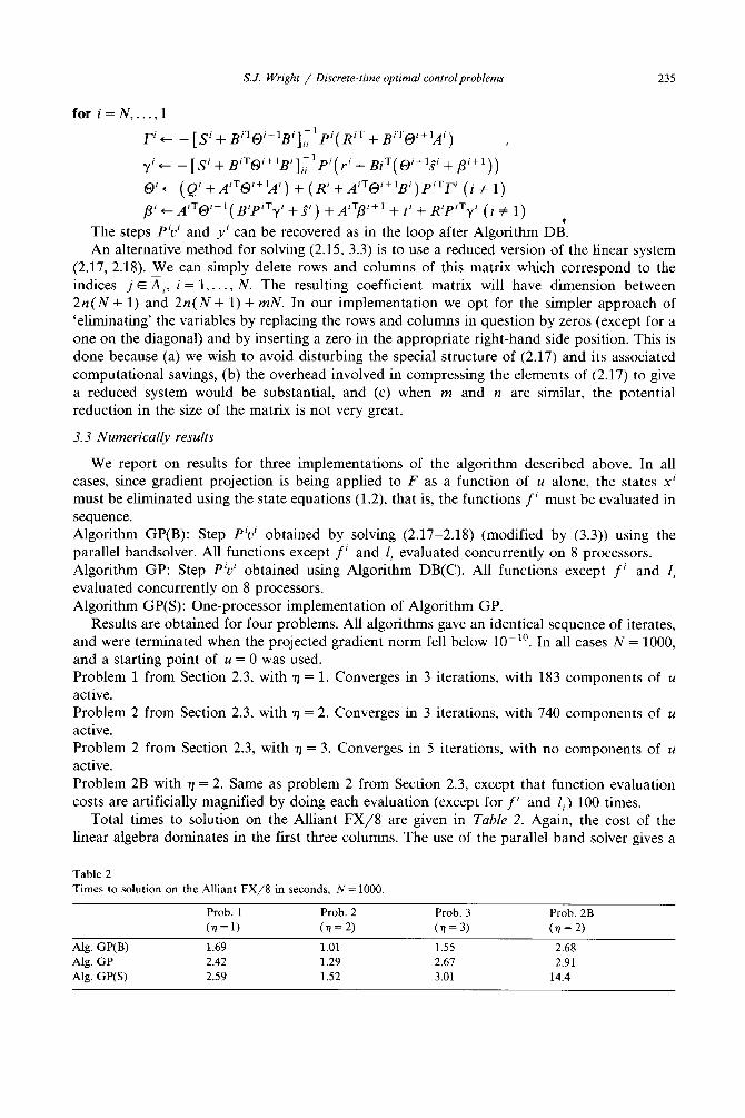
The steps pivi and yi can be recovered as in the loop after Algorithm DB. An alternative method for solving (2.15, 3.3) is to use a reduced version of the linear system

(2.17, 2.18). We can simply delete rows and columns of this matrix which correspond to the indices j ~ Ai, i = 1 . . . . . N. The resulting coefficient matrix will have dimension between 2 n ( N + 1) and 2 n ( N + 1 ) + raN. In our implementation we opt for the simpler approach of 'eliminating' the variables by replacing the rows and columns in question by zeros (except for a one on the diagonal) and by inserting a zero in the appropriate right-hand side position. This is done because (a) we wish to avoid disturbing the special structure of (2.17) and its associated computational savings, (b) the overhead involved in compressing the elements of (2.17) to give a reduced system would be substantial, and (c) when m and n are similar, the potential reduction in the size of the matrix is not very great.

3.3 Numerically results

We report on results for three implementations of the algorithm described above. In all cases, since gradient projection is being applied to F as a function of u alone, the states x ~ must be eliminated using the state equations (1.2), that is, the functions f~ must be evaluated in sequence. Algorithm GP(B): Step piv~ obtained by solving (2.17-2.18) (modified by (3.3)) using the parallel bandsolver. All functions except f~ and l~ evaluated concurrently on 8 processors. Algorithm GP: Step pivi obtained using Algorithm DB(C). All functions except f i and I~ evaluated concurrently on 8 processors. Algorithm GP(S): One-processor implementation of Algorithm GP.

Results are obtained for four problems. All algorithms gave an identical sequence of iterates, and were terminated when the projected gradient norm fell below 10-~0. In all cases N = 1000, and a starting point of u = 0 was used. Problem 1 from Section 2.3, with 77 = 1. Converges in 3 iterations, with 183 components of u active. Problem 2 from Section 2.3, with 7/= 2. Converges in 3 iterations, with 740 components of u active. Problem 2 from Section 2.3, with 7/= 3. Converges in 5 iterations, with no components of u active. Problem 2B with ~/= 2. Same as problem 2 from Section 2.3, except that function evaluation costs are artificially magnified by doing each evaluation (except for fs and 1~) 100 times.

Total times to solution on the Alliant F X / 8 are given in Table 2. Again, the cost of the linear algebra dominates in the first three columns. The use of the parallel band solver gives a

Table 2 Times to solution on the Alliant FX/8 in seconds, N = 1000.

Prob. 1 Prob. 2 Prob. 3 Prob. 2B (n =1) (~/= 2) (~1 = 3) (~7 = 2)

Alg. GP(B) 1.69 1.01 1.55 2.68 Alg. GP 2.42 1.29 2.67 2.91 Alg. GP(S) 2.59 1.52 3.01 14.4


speedup of somewhat less than that obtained for the corresponding unconstrained problems. This can be attributed to the fact (mentioned above) that the band solver in Algorithm GP(P) does not at present take advantage of the reduced dimension of the Newton step. (Hence the fewer constraints active, the better the speedup - compare the second and third columns.) Best results are obtained for Problem 2B, which is meant to typify applications in which the state equations f i are easily evaluated (e.g. linear), but evaluation of the objective functions and their derivatives is expensive. A speedup of 5.4 is obtained by the best parallel algorithm GP(B) over the best sequential algorithm GP(S).

3.4 A hybrid approach

As noted above, the need for evaluation of the nonlinear state equations (1.2) between iterations of the gradient projection method presents a possible serial bottleneck in the simple control-constrained case, since this entails evaluating the functions f i in sequence. A poten- tially more parallelizable approach would be to use a two-level method. Sequential quadratic programming (IQP variant) could be applied to the original nonlinear problem (1.1, 1.2, 1.4), yielding a subproblem in which the state equations are linear, and in which the bound constraints (1.4) still appear. This subproblem could then be solved using a gradient projection method. The state equations still need to be evaluated between each gradient projection iteration, but since they are now linear, this step can be implemented in parallel using much the same techniques which were used to parallelize the banded system solver.

4. Conclusions and further work

We have discussed multiprocessor implementations of some basic rapidly-convergent algorithms for discrete-time optimal control problems, which attempt to exploit parallelism both in the linear algebra and in evaluation of the functions. Further work remains to be done to implement these methods on message-passing machines (e.g. hypercubes and massively parallel architectures). Additionally, algorithms with better global convergence properties are needed. Simple techniques for ensuring global convergence of Newton's method and gradient projection methods are quite well understood; for SQP more complicated devices are needed. The challenge is to implement the globalization strategies without interfering too much with the parallelism which has been obtained in the basic algorithms above.

References

[1] D.P. Bertsekas, Projected Newton methods for optimization problems with simple constraints, SlAM J. Control Optim. 20 (1982) 221-246.

[2] G. Di Pillo, L. Grippo and F. Lampariello, A class of structured quasi-Newton algorithms for optimal control problems, in: Proc. IFAC Applications of Nonlinear Programming to Optimization and Control (1983).

[3] J. Dunn, A projected Newton method for minimization problems with nonlinear inequality constraints, Numer. Math. 53 (1988) 377-409.

[4] J. Durra and D.P. Bertsekas, Efficient dynamic programming implementations of Newton's method for unconstrained optimal control problems, J. Optim. Theory Appl., 63 (1989) 23-38.

[5] R. Fletcher, Practical Methods of Optimization (2nd edition) (Wiley, New York, 1987). [6] E.M. Gafni and D.P. Bertsekas, Two-metric projection methods for constrained optimization, SlAM J. Control

Optim. 22 (1984) 936-964. [7] D.H. Jacobson and D.Q. Mayne, Differential Dynamic Programming (American Elsevier, New York, 1970). [8] C.T. Kelley and E.W. Sachs, A pointwise quasi-Newton method for unconstrained optimal control problems,

Numer. Math. 55 (1989) 159-176.


[9] K. Ohno, A new approach to differential dynamic programming for discrete time systems, IEEE Trans. Automat. Control AC-23 (1978) 37-47.

[10] J.F.A. Pantoja and D.Q. Mayne, A sequential quadratic programming algorithm for discrete optimal control problems with control inequality constraints, submitted, 1988.

[11] L.J. Podrazik and G.G.L. Meyer, A parallel first-order linear recurrence solver, J. Parallel Dist. Comp. 4 (1987) 117-132.

[12] E. Polak, Computational Methods in Optimization (Academic Press, New York, 1970). [13] M.J.D. Powell, ed., Nonlinear Optimization 1981 (Academic Press, New York, 1982). [14] S.J. Wright, Parallel algorithms for banded linear systems, Argonne National Laboratory Preprint MCS-P64-0289,

1989, SIAM J. Sci. Statist. Comput., to appear.

Documents

Solution of discrete-time optimal control problems on ...pages.cs.wisc.edu/~swright/papers/WrightParallelComputing90.pdf · Solution of discrete-time optimal control problems on parallel