Embed Size (px)
Citation preview

Solution of nonlinear Riccati differentialequation using Chebyshev wavelets
S. BALAJIDepartment of Mathematics
SASTRA UniversityThanjavur - 613 401
INDIAbalaji [email protected]
Abstract: A generalized Chebyshev wavelet operational matrix (CWOM) is presented for the solution of nonlin-ear Riccati differential equations. The operational matrix together with suitable collocation points converts thefractional order Riccati differential equations into a system of algebraic equations. Accuracy and efficiency of theproposed method is verified through numerical examples and comparison with the recently developed approaches.The obtained results reveal that the performance of the proposed method is more accurate and reliable.
Key–Words: Riccati equation, Nonlinear ODE, Chebyshev wavelet, convergence, operational matrix.
1 IntroductionIn this paper we consider the fractional-order Riccatidifferential equation of the form
Dαy(t) = P (t)y2 +Q(t)y +R(t), t > 0,
α ∈ (0, 1) with the initial condition
y(0) = k.
when α = 1, the above equation is called classicalRiccati differential equation and these equations willbe investigated.
The Riccati differential equations (RDEs) haslarge variety of applications in engineering and ap-plied science such as damping laws, rheology, diffu-sion processes, transmission line phenomena, optimalcontrol theory problems etc., [1, 2, 3, 4, 5, 6]. It is tobe noted that the RDEs are complicated in its struc-ture and finding exact solutions for them cannot besimple. Applications and structure of RDEs attractedresearchers to develop efficient methods to solve themin order to get more accurate solutions.
A substantial amount of research work has beendone in the development of solution of RDEs. Themost significant methods are Adomian decomposi-tion method [7], homotopy perturbation method [8-11], homotopy analysis method [12, 13], Taylor ma-trix method [14] and Haar wavelet method [15], com-bination of Laplace, Adomian decomposition and Padapproximation [16] methods.
Several numerical methods for approximating thesolution of nonlinear fractional-order Riccati differ-ential equations equation are known. Raja et.al [17]
developed a stochastic technique based on particleswarm optimization and simulated annealing. Theywere used as a tool for rapid global search method andsimulated annealing for efficient local search method.A fractional variational iteration method described inthe Riemann-Liouville derivative has been applied in[18], to give an analytical approximate solution tononlinear fractional Riccati differential equation. ACombination of finite difference method and Pade? -variational iteration numerical scheme was proposedby Sweilam et. al [19]. Moreover an analyticalscheme comprising the Laplace transform, the Ado-mian decomposition method (ADM), and the Pad ap-proximation given in [16].
However, the above mentioned methods havesome restrictions and disadvantages in their perfor-mance. For example, very complicated and tough-est adomian polynomials are constructed in the Ado-mian decomposition method. In the variational itera-tion method identification Lagrange multiplier yieldsan underlying accuracy. The homotopy perturbationmethod needs a linear functional equation in each it-eration to solve nonlinear equations, forming thesefunctional equations are very difficult. The perfor-mance of the homotopy analysis method is very muchdepends on the chosen of the auxiliary parameter h ofthe zero-order deformation equation. Moreover, theconvergence region and implementation of these re-sults are very small.
In recent years, wavelets theory is one of thegrowing and predominantly a new method in the areaof mathematical and engineering research. It has been
WSEAS TRANSACTIONS on MATHEMATICS S. Balaji
E-ISSN: 2224-2880 441 Volume 13, 2014
applied in vast range of engineering sciences, partic-ularly, they are used very successfully for waveformrepresentation and segmentations in signal analysis,time-frequency analysis and in the mathematical sci-ences it is used in thriving manner for solving varietyof linear and non linear differential and partial differ-ential equations and fast algorithms for easy imple-mentation [20]. Moreover wavelets build a connectionwith fast numerical algorithms [21, 29], this is due towavelets admit the exact representation of a variety offunction and operators. The application of Chebyshevwavelets are thoroughly considered in [22, 23].
In this work, the nonlinear Riccati differen-tial equations of fractional-order approached analyt-ically by using Chebyshev wavelets operational ma-trix (CWOM) method. The operational matrix ofChebyshev wavelet is generalized for fractional cal-culus in order to solve fractional and classical Ric-cati differential equations. The proposed CWOMmethod is illustrated by application, and obtained re-sults are compared with recently proposed method forthe fractional-order Riccati differential equation. Wehave adopted Chebyshev wavelet method to solve Ric-cati differential equations not only due to its emergingapplication of but also due to its greater convergenceregion.
The rest of the paper is as follows: In section2 definitions and mathematical preliminaries of frac-tional calculus are presented. In section 3 Cheby-shev wavelet, its properties, function approximationsand generalized Chebyshev wavelet operational ma-trix fractional calculus are discussed. Section 4 estab-lishes application of proposed method in the solutionRiccati differential equations, existence and unique-ness solution of the proposed problem and conver-gence analysis of the proposed approach. Section 5deals with the illustrative examples and their solutionsby the proposed approach. Section 6 ends with ourconclusion.
2 Preliminaries and notations
The notations, definitions and preliminary factspresent in this section will be used in forthcomingsections of this work. Several definitions of frac-tional integrals and derivatives have been proposed af-ter the logical definition given by Liouville. Impor-tant and few of these definitions include the Riemann-Liouville, the Caputo, the Weyl, the Hadamard, theMarchaud, the Riesz, the Grunwald-Letnikov andthe Erdelyi-Kober. The Caputo fractional derivativeuses initial and boundary conditions of integer orderderivatives having some physical interpretations. Be-cause of this specific reason, in this work we shall use
the Caputo fractional derivative proposed by Caputo[24] in the theory of viscoelasticity.
The Caputo fractional derivative of order α >0, (α ∈ R, n − 1 < α ≤ n, n ∈ N) and h :(0,∞) −→ R is continuous is defined by
Dαf(t) = In−α(dn
dtnf(t)
)(1)
where
Iαf(t) =1
Γ(α)
∫ t
0(t− s)α−1f(s) ds (2)
is the Riemann-Liouville fractional integral operatorof order α > 0 and Γ is the gamma function. Thefractional integral of tβ , β > −1is given as
Iα(t− α)β =Γ(β + 1)
Γ(β + α+ 1)(t− a)β+α, a ≥ 0 (3)
Properties of fractional integrals and derivatives are asfollows [25], for α, β > 0:
The fractional order integral satisfies the semigroup property
Iα(Iβf(t)
)= Iβ (Iαf(t)) = Iα+βf(t) (4)
The integer order derivative Dn and fractional orderderivative Dα commute with each other,
Dn (Dαf(t)) = Dα (Dnf(t)) = Dα+nf(t) (5)
The fractional integral operator and fractional deriva-tive operator do not satisfy the commutative property.In general,
Iα (Dαf(t)) = f(t)−n−1∑k=0
fk(0)tk
k!(6)
but in the reverse way we have
Dα(Iβf(t)
)= Dα−βf(t) (7)
3 Properties of Chebyshev waveletsand its operational matrix of frac-tional integration
A family of functions constituted by Wavelets, con-structed from dilation and translation of a single func-tion called mother wavelet. When the parameters aof dilation and b of translation vary continuously, fol-lowing are the family of continuous wavelets [26]
ψa,b(t) = |a|−1/2 ψ
(t− ba
), a, b ∈ R, a = 0.
WSEAS TRANSACTIONS on MATHEMATICS S. Balaji
E-ISSN: 2224-2880 442 Volume 13, 2014
If the parameters a and b are restricted to discrete val-ues as a = a−k0 , b = nb0a
−k0 , a0 > 1, b0 > 0 and n,
and k are positive integers, following are the family ofdiscrete wavelets:
ψk,n(t) = |a0|k/2 ψ(ak0t− nb0
)where ψk,n(t) form a wavelet basis for L2(R) . Inparticular, when a0 = 2, and b0 = 1, ψk,n(t) formsan orthonormal basis [26].
Chebyshev wavelets ψk,n(t) = ψ(k, n,m, t)
have four arguments; n = 1, 2, 3, . . . 2k−1, k can as-sume any positive integer, m is the degree of Cheby-shev polynomials of first kind and t denotes the nor-malized time. They are defined on the interval [0, 1)as [27, 28]
ψnm(t) =
αm2(k+1)/2
√π
Tm(2kt− 2n+ 1)
for n−12k−1 ≤ t < n
2k−1
0, otherwise
where
αm =
{ √2 for m = 0
2 for m = 1, 2, . . .
and m = 0, 1, . . . ,M − 1 and n = 1, 2, 3, . . . , 2k−1.Tm(t) are the well-known Chebyshev polynomials oforder m defined on the interval [-1, 1], which are or-thogonal with respect to the weight function ω(t) =
1 ∧√1− x2 and they can be determined with the aid
of the following recurrence formulae:
T0(t) = 1, T1(t) = t,Tm+1(t) = 2tTm(t)− Tm−1(t), m = 1, 2, 3, . . .
The Chebyshev wavelet series representation of thefunction f(t) defined over [0, 1) is given by
f(t) =∞∑n=1
∞∑m=0
cnmψnm(t) (8)
where cnm = ⟨f(t), ψnm(t)⟩, in which ⟨., .⟩ denotesthe inner product. If the infinite series in Eq. (8) istruncated, then Eq. (8) can be written as
f(t) =2k−1∑n=1
M−1∑m=0
cnmψnm(t) = CTΨ(t) = f(t) (9)
where C and Ψ(t) are 2k−1M × 1 matrices given by
C =
[c10, c11, . . . , c1M−1, c20, c21, . . . , c2M−1,· · · , c2k−10, c2k−11, . . . , c2k−1M−1
]T
and
Ψ(t) =
ψ10(t) ψ11(t) . . . ψ1M−1(t),ψ20(t) ψ21(t) . . . ψ2M−1(t),
... · · · · · ·...
ψ2k−10(t) ψ2k−11(t) . . . ψ2k−1M−1(t)
T
(10)Taking suitable collocation points as following
ti =(2i− 1)
2kM, i = 1, 2, . . . , 2k−1M,
we defined the m-square Chebyshev matrix
ϕm×m =
[Ψ
(1
2kM
),Ψ
(3
2kM
), . . . ,Ψ
(2kM−12kM
)]
where m = 2k−1M , correspondingly we have
f =[f(
12kM
), f(
32kM
), . . . , f
(2kM−12kM
)]= CTϕm×m
The Chebyshev matrix ϕm×m is an invertible ma-trix, the coefficient vector CT is obtained by CT =
fϕ−1m×m.
3.1 Operational matrix of the fractional in-tegration
The integration of the Ψ(t) defined in Eq.(10) canbe approximated by Chebyshev wavelet series withChebyshev wavelet coefficient matrix P∫ t
0Ψ(t)dt = Pm×mΨ(t)
where P is called Chebyshev wavelet operational ma-trix of integration.
The m-set of Block Pulse Functions is defined on[0, l) as follows
bi(t) =
{1, i
m ≤ t <(i+1)m
0, otherwise
where i = 0, 1, 2, . . . ,mThe functions bi are disjoint and orthogonal. That is,
bi(t)bj(t) =
{bi(t), i = j0, i = j
and ∫ 1
0bi(t)bj(t)dt =
{1m , i = j0, i = j
WSEAS TRANSACTIONS on MATHEMATICS S. Balaji
E-ISSN: 2224-2880 443 Volume 13, 2014
The orthogonality property of block-pulse func-tion is obtained from the disjointness property. Anarbitrary function f ∈ L2[0, 1), can be expanded intoblock-pulse functions as
f(t) ≈m−1∑i=0
fibi(t) = fTB(t)
where fi are the coefficients of the block-pulse func-tion, given by
fi =m
l
∫ l
0f(t)bi(t)dt
The Chebyshev wavelets can be expanded into m-setof block-pulse functions as
Ψ(t) = ϕm×mB(t) (11)
where B(t) = [b0(t), b1(t), · · · , bi(t), · · · , bm−1(t)]T .
The fractional integral of block-pulse functionvector can be written as
(IαB) (t) = Fαm×mB(t) (12)
where Fαm×m is given in [27].Now we derive the Chebyshev wavelet opera-
tional matrix of the fractional integration
(IαΨ) (t) ≈ Pαm×mΨ(t) (13)
where the m - square matrix Pm×m is called Cheby-shev wavelet operational matrix of the fractional inte-gration.
Using Eqs. (11) and (13) we have
(IαΨ) (t) ≈ (Iαϕm×mB) (t)
= ϕm×m (IαB) (t) ≈ ϕm×m (FαB) (t)(14)
From Eqs. (13) and (14) we get
Pαm×mΨ(t) = ϕm×mFαB(t) (15)
and by the Eq. (11), the Eq. (15) becomes
Pαm×mϕm×mB(t) = ϕm×mFαB(t) (16)
Then the Chebyshev wavelet operational matrixPαm×m of fractional integration is given by
Pαm×m = ϕm×mFαϕ−1
m×m (17)
Following is the Chebyshev wavelet operational ma-trix Pαm×m of fractional order integration, for the par-ticular values of k = 2,M = 3, α = 0.5
P 0.56×6 =
0.5415 0.4324 0.1819 −0.0871 −0.0179 0.01540 0.5415 0 0.1819 0 −0.0179
−0.2046 0.071 0.2243 −0.0449 0.0798 0.01190 −0.2046 0 0.2243 0 0.0798
0.1781 0.2506 −0.0252 −0.0652 0.1555 0.01430 0.1781 0 −0.0252 0 0.1555
4 Application to fractional Riccatidifferential Equation
In this section, we will use the generalized Chebyshevwavelet operational matrix to solve nonlinear Ric-cati differential equation and we discuss the existenceand uniqueness of solutions with initial conditionsand convergence criteria of the proposed CWOM ap-proach.
Consider the fractional-order Riccati differentialequation of the form
Dαy(t) = P (t)y2 +Q(t)y +R(t), t > 0, (18)
0 < α ≤ 1 with the initial condition
y(0) = k. (19)
Let us suppose that the functions Dαy(t) ,P (t), Q(t), R(t) are approximated using Chebyshevwavelet as follows:
Dαy(t) = UTΨ(t), P (t) = V TΨ(t)Q(t) =W TΨ(t), R(t) = XTΨ(t)
(20)
where U, V,W,X and Ψ(t) are given in Eqs. (10).Using the Eq.(6), we can write
y(t) = Iα (Dαy(t))− y(0) (21)
By the Eqs. (13) and (19), the Eq. (21) leads to
y(t) ≈ UTPαm×mΨ(t) + Y T0 (t)Ψ(t) = CTΨ(t)
(22)where
y(0) = k ≈ Y T0 (t)Ψ(t), C =
(UTPαm×m + Y T
0
)TSubstituting Eqs. (20) and (22) into Eq.(18), we have
UTΨ(t) = V TΨ(t)[CTΨ(t)
]2+W TΨ(t)CTΨ(t) +XTΨ(t)
(23)
Substituting Eq. (11) into the Eq. (23), we have
UTϕm×m = V T[CTϕm×m
]2+W TCTϕm×m +XT
(24)
where C, V,W and ϕm×m are known. Eq. (24) repre-sents a system of nonlinear equations with unknownvector U . This system of nonlinear equations can besolved by Newton method for the unknown vector Uand we can get the approximation solution by includ-ing U into Eq.(22).
WSEAS TRANSACTIONS on MATHEMATICS S. Balaji
E-ISSN: 2224-2880 444 Volume 13, 2014
4.1 Existence and uniqueness of solutions
Consider the fractional-order Riccati differentialequation of the form of Eqs.(18) and (19). The non-linear term in Eq. (18) is y2 and P (t), Q(t), R(t) areknown functions. For α = 1, the fractional-orderRiccati converts into the classical Riccati differentialequation.
Definition 1 Let I = [0, l], l < ∞ and C(I) be theclass of all continuous function defined on I , with thenorm
∥y∥ = supt∈I
∣∣∣e−hty(t)∣∣∣ , h > 0
which is equivalent to the sup-norm of y.
Remark 2 Assume that solution y(t) offractional-order Riccati differential Eqs.(18) and (19) belongs to the space S ={y ∈ R : |y| ≤ c, c is any constant}, in orderto study the existence and uniqueness of the initialvalue problem.
Definition 3 The Space of integrable functionsL1[0, l] in the interval [0, l] is defined as
L1[0, l] =
{u(t) :
∫ l
0|u(t)|dt <∞
}.
Theorem 4 The initial value problem given by Eqs.(18) and (19) has a unique solution
y ∈ C(I), y′ ∈{y ∈ L1[0, l], ∥y∥ =
∣∣∣e−hty(t)∣∣∣L1
}Proof: By Eq. (1), the fractional differential Eq. (18)can be written as
I1−αdy(t)
dt= P (t)y2 +Q(t)y +R(t) (25)
becomes
y(t) = Iα(P (t)y2 +Q(t)y +R(t)
)(26)
Now we define the operator Θ : C(I) −→ C(I) by
Θy(t) = Iα(P (t)y2 +Q(t)y +R(t)
)(27)
then,
e−ht (Θy −Θw)
= e−htIα[(P (t)y2 +Q(t)y +R(t))−(P (t)w2 +Q(t)w +R(t))
]
≤ 1Γ(α)
∫ t0
((t− s)α−1e−h(t−s)
((y − w)(y + w)− k(y − w)) e−hs
)ds
≤ ∥y − w∥ 1Γ(α)
∫ t0 s
α−1e−hsds
hence, we have
∥Θy −Θw∥ < ∥y − w∥
which implies the operator given by Eq. (27), has aunique fixed point and consequently the given integralequation has a unique solution y ∈ C(I) . Also wecan see that
IαP (t)y2 +Q(t)y +R(t)|t=0 = k (28)
Now from Eq. (26), we have
y(t) =
[tα
Γ(α+1)(Py20 +Qy0 +R)+
Iα+1(P ′y2 + 2y′P +Q′y +Qy′ +R′)
]
and
dy
dt=
[tα−1
Γ(α) (Py20 +Qy0 +R)+
Iα(P ′y2 + 2y′P +Q′y +Qy′ +R′)
]
e−htdy
dt= e−ht
[tα−1
Γ(α) (Py20 +Qy0 +R)+
Iα(P ′y2 + 2y′P +Q′y +Qy′ +R′)
]from which we can deduce that y′ ∈ C(I) and y′ ∈ SNow again from Eqs. (26), (27) and (28) we get
dy
dt=
d
dtIα[Py2 +Qy +R]
I1−α dydt = I1−α ddtI
α[Py2 +Qy +R]
= ddtI
1−αIα[Py2 +Qy +R]
Dαy(t) = ddtI[Py
2 +Qy +R]= Py2 +Qy +R
andy(0) = IαPy2 +Qy +R|t=0 = k
which implies that the integral equation (28) is equiv-alent to the initial value problem (19) and the theoremis proved.
4.2 Convergence analyses
Letψk,n(t) = |a0|k/2 ψ
(ak0t− nb0
)where ψk,n(t) form a wavelet basis for L2(R) . Inparticular, when a0 = 2, and b0 = 1, ψk,n(t) formsan orthonormal basis [26].
Let
y(t) =M−1∑i=1
c1iψ1i(t)
WSEAS TRANSACTIONS on MATHEMATICS S. Balaji
E-ISSN: 2224-2880 445 Volume 13, 2014
be the solution of the Eq. (18) where c1i =⟨y(t), ψ1i(t)⟩ for k = 1 in which ⟨., .⟩ denotes theinner product.
y(t) =n∑i=1
⟨y(t), ψ1i(t)⟩ψ1i(t) (29)
Let βj = ⟨y(t), ψ(t)⟩ where
ψ(t) = ψ1i(t) (30)
Let xn =∑nj=1 βjψ(tj) be a sequence of partial
sums. Then,
⟨y(t), xn⟩ =⟨y(t),
n∑j=1
βjψ(tj)
⟩=
n∑j=1
βj ⟨y(t), ψ(tj)⟩
=n∑j=1
βjβj =n∑j=1|βj |2
Further
∥xn − xm∥2 =∥∥∥∑n
j=m+1 βjψ(tj)∥∥∥2
=
⟨n∑
i=m+1βiψ(ti),
n∑j=m+1
βjψ(tj)
⟩=
n∑i=m+1
n∑j=m+1
βiβj ⟨ψ(ti), ψ(tj)⟩
=n∑
j=m+1|βj |2
As n → ∞ , from Bessel’s inequality, we have∑∞j=1 |βj |2 is convergent. It implies that xn is a
Cauchy sequence and it converges to x (say).Also
⟨x− y(t), ψ(tj)⟩ = ⟨x, ψ(tj)⟩ − ⟨y(t), ψ(tj)⟩= ⟨Ltn→∞xn, ψ(tj)⟩ − βj= Ltn→∞ ⟨xn, ψ(tj)⟩ − βj
= Ltn→∞
⟨n∑j=1
βjψ(tj), ψ(tj)
⟩− βj
= βj − βj= 0.
which is possible only if y(t) = x. i.e., both y(t) andxn converges to the same value, which indeed give theguarantee of convergence of CWOM.
5 Numerical Examples
In order to show the effectiveness of the Chebyshevwavelets operational matrix method (CWOM), we im-plement CWOM to the nonlinear fractional Riccati
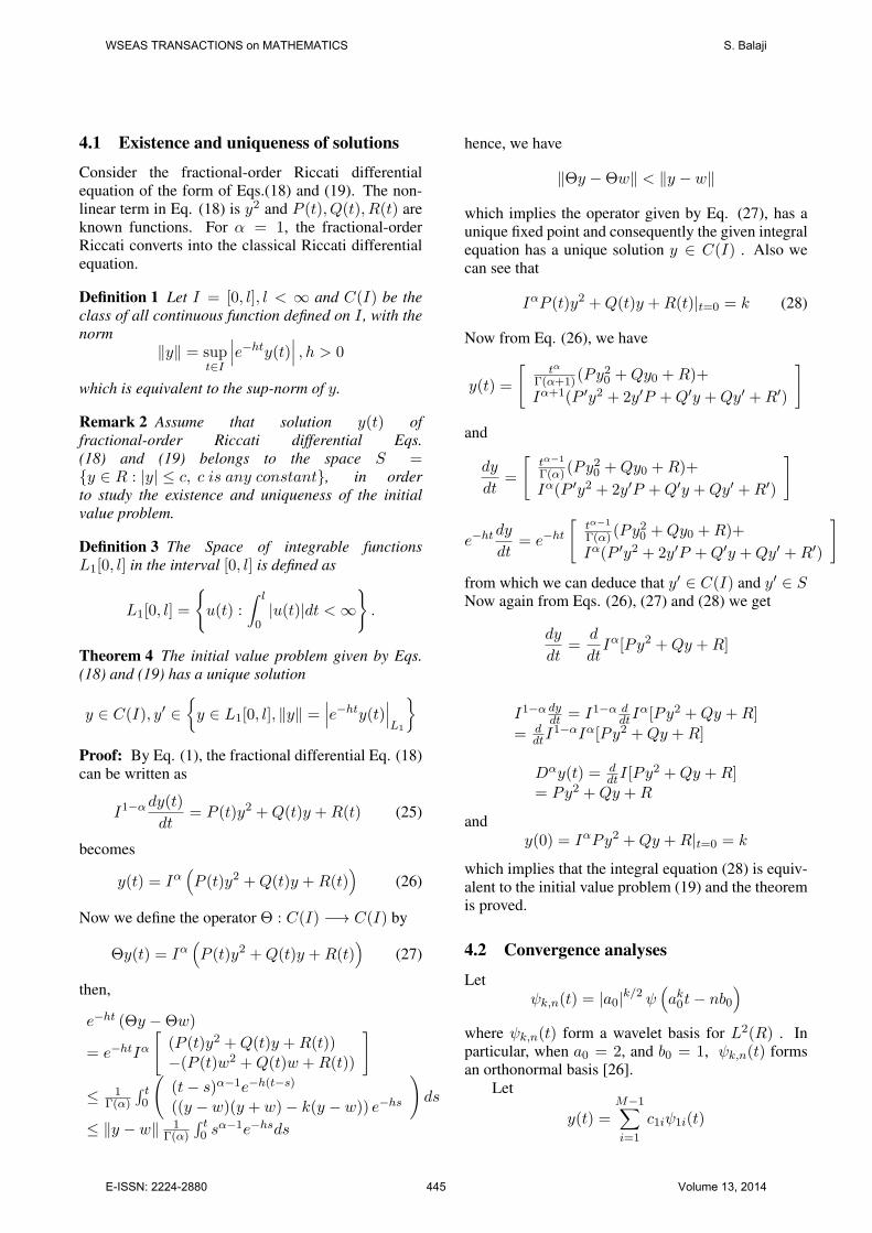
Figure 1: Numerical Results of Example 5 by CWOMfor α = 1
differential equations. All the numerical experimentscarried out on a personal computer with some MAT-LAB codes. The specification of PC is intel core i5processor and with Turbo boost up to 3.1GHz and4 GB of DDR3 memory. The following problemsof nonlinear Riccati differential equations are solvedwith real coefficients.
Example 5 Consider the following nonlinear frac-tional Riccati differential equation
Dαy(t) = 1 + 2y(t)− y2(t), 0 < α ≤ 1 (31)
with initial condition
y(0) = 0 (32)
Exact solution for α = 1 was found to be
y(t) = 1 +√2 tanh
(√2t+
1
2log
√2− 1√2 + 1
)
The integral representation of the Eqs.(31) and(32) is given by
Iα (Dαy(t)) = Iα(1 + 2y(t)− y2(t)
)y(t) = y(0) +
tα
Γ(α+ 1)+ 2Iαy(t)− Iαy2(t) (33)
Lety(t) = CTΨ(t) (34)
thenIαy(t) = CT IαΨ(t)= CTPα
2k−1M×2k−1MΨ(t)
(35)
WSEAS TRANSACTIONS on MATHEMATICS S. Balaji
E-ISSN: 2224-2880 446 Volume 13, 2014
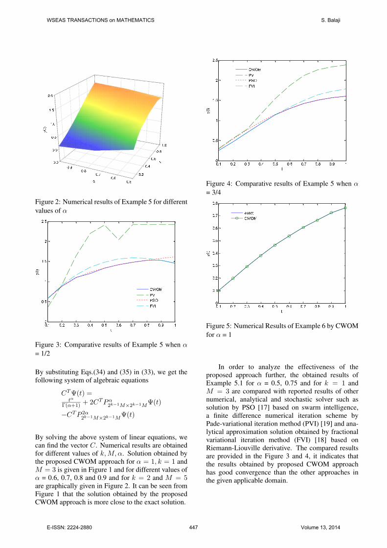
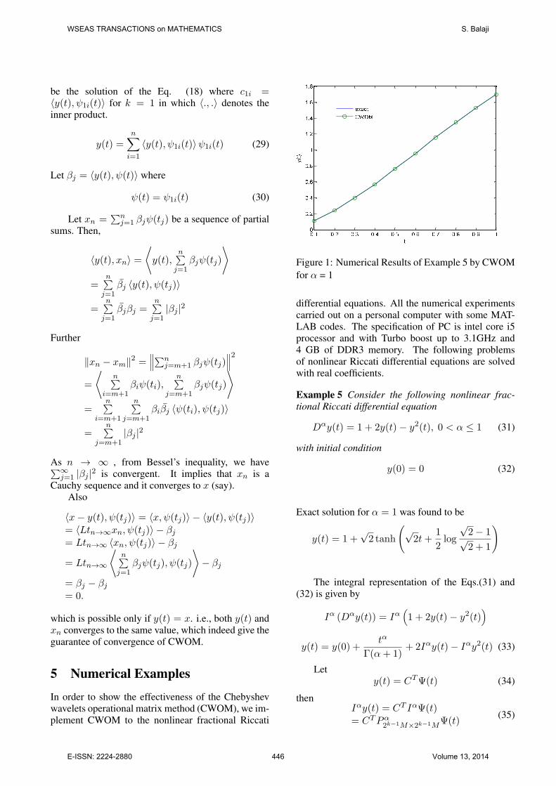
Figure 2: Numerical results of Example 5 for differentvalues of α
Figure 3: Comparative results of Example 5 when α= 1/2
By substituting Eqs.(34) and (35) in (33), we get thefollowing system of algebraic equations
CTΨ(t) =tα
Γ(α+1) + 2CTPα2k−1M×2k−1M
Ψ(t)
−CTP 2α2k−1M×2k−1M
Ψ(t)
By solving the above system of linear equations, wecan find the vector C. Numerical results are obtainedfor different values of k,M,α. Solution obtained bythe proposed CWOM approach for α = 1, k = 1 andM = 3 is given in Figure 1 and for different values ofα = 0.6, 0.7, 0.8 and 0.9 and for k = 2 and M = 5are graphically given in Figure 2. It can be seen fromFigure 1 that the solution obtained by the proposedCWOM approach is more close to the exact solution.
Figure 4: Comparative results of Example 5 when α= 3/4
Figure 5: Numerical Results of Example 6 by CWOMfor α = 1
In order to analyze the effectiveness of theproposed approach further, the obtained results ofExample 5.1 for α = 0.5, 0.75 and for k = 1 andM = 3 are compared with reported results of othernumerical, analytical and stochastic solver such assolution by PSO [17] based on swarm intelligence,a finite difference numerical iteration scheme byPade-variational iteration method (PVI) [19] and ana-lytical approximation solution obtained by fractionalvariational iteration method (FVI) [18] based onRiemann-Liouville derivative. The compared resultsare provided in the Figure 3 and 4, it indicates thatthe results obtained by proposed CWOM approachhas good convergence than the other approaches inthe given applicable domain.
WSEAS TRANSACTIONS on MATHEMATICS S. Balaji
E-ISSN: 2224-2880 447 Volume 13, 2014
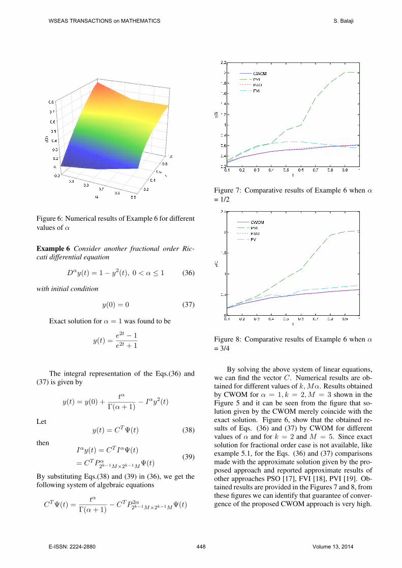
Figure 6: Numerical results of Example 6 for differentvalues of α
Example 6 Consider another fractional order Ric-cati differential equation
Dαy(t) = 1− y2(t), 0 < α ≤ 1 (36)
with initial condition
y(0) = 0 (37)
Exact solution for α = 1 was found to be
y(t) =e2t − 1
e2t + 1
The integral representation of the Eqs.(36) and(37) is given by
y(t) = y(0) +tα
Γ(α+ 1)− Iαy2(t)
Lety(t) = CTΨ(t) (38)
thenIαy(t) = CT IαΨ(t)
= CTPα2k−1M×2k−1M
Ψ(t)(39)
By substituting Eqs.(38) and (39) in (36), we get thefollowing system of algebraic equations
CTΨ(t) =tα
Γ(α+ 1)− CTP 2α
2k−1M×2k−1MΨ(t)
Figure 7: Comparative results of Example 6 when α= 1/2
Figure 8: Comparative results of Example 6 when α= 3/4
By solving the above system of linear equations,we can find the vector C. Numerical results are ob-tained for different values of k,Mα. Results obtainedby CWOM for α = 1, k = 2,M = 3 shown in theFigure 5 and it can be seen from the figure that so-lution given by the CWOM merely coincide with theexact solution. Figure 6, show that the obtained re-sults of Eqs. (36) and (37) by CWOM for differentvalues of α and for k = 2 and M = 5. Since exactsolution for fractional order case is not available, likeexample 5.1, for the Eqs. (36) and (37) comparisonsmade with the approximate solution given by the pro-posed approach and reported approximate results ofother approaches PSO [17], FVI [18], PVI [19]. Ob-tained results are provided in the Figures 7 and 8, fromthese figures we can identify that guarantee of conver-gence of the proposed CWOM approach is very high.
WSEAS TRANSACTIONS on MATHEMATICS S. Balaji
E-ISSN: 2224-2880 448 Volume 13, 2014
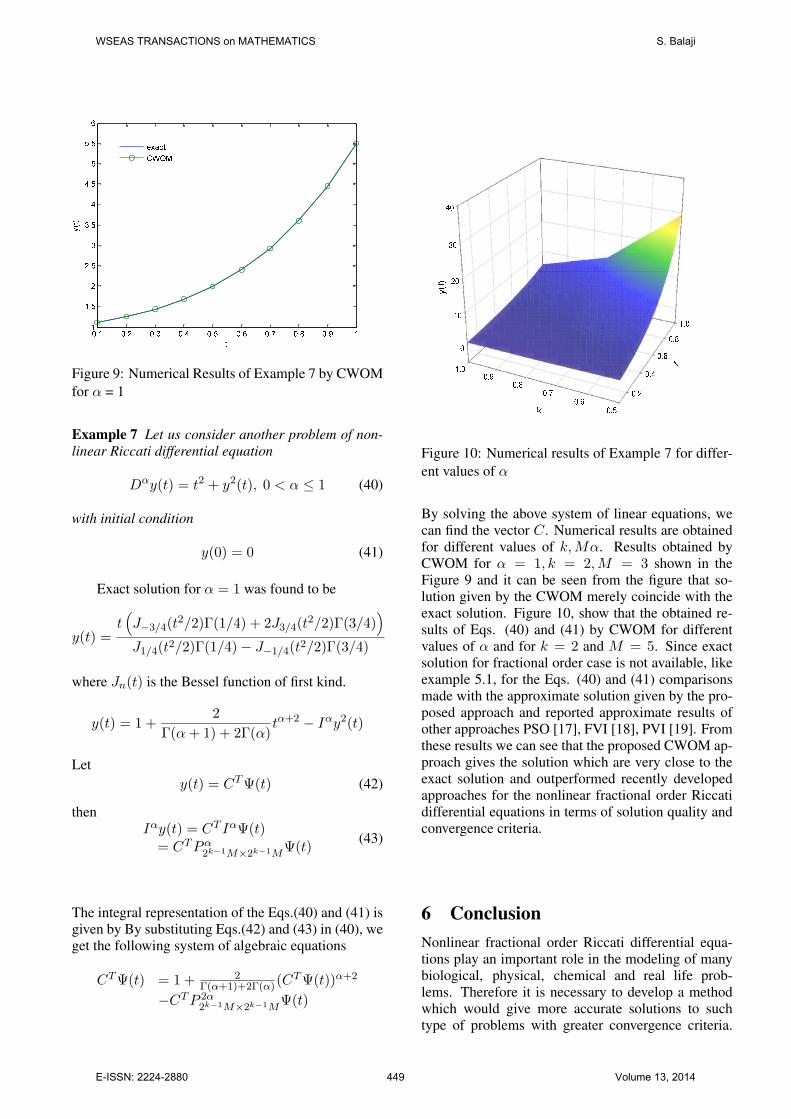
Figure 9: Numerical Results of Example 7 by CWOMfor α = 1
Example 7 Let us consider another problem of non-linear Riccati differential equation
Dαy(t) = t2 + y2(t), 0 < α ≤ 1 (40)
with initial condition
y(0) = 0 (41)
Exact solution for α = 1 was found to be
y(t) =t(J−3/4(t
2/2)Γ(1/4) + 2J3/4(t2/2)Γ(3/4)
)J1/4(t2/2)Γ(1/4)− J−1/4(t2/2)Γ(3/4)
where Jn(t) is the Bessel function of first kind.
y(t) = 1 +2
Γ(α+ 1) + 2Γ(α)tα+2 − Iαy2(t)
Lety(t) = CTΨ(t) (42)
thenIαy(t) = CT IαΨ(t)
= CTPα2k−1M×2k−1M
Ψ(t)(43)
The integral representation of the Eqs.(40) and (41) isgiven by By substituting Eqs.(42) and (43) in (40), weget the following system of algebraic equations
CTΨ(t) = 1 + 2Γ(α+1)+2Γ(α)(C
TΨ(t))α+2
−CTP 2α2k−1M×2k−1M
Ψ(t)
Figure 10: Numerical results of Example 7 for differ-ent values of α
By solving the above system of linear equations, wecan find the vector C. Numerical results are obtainedfor different values of k,Mα. Results obtained byCWOM for α = 1, k = 2,M = 3 shown in theFigure 9 and it can be seen from the figure that so-lution given by the CWOM merely coincide with theexact solution. Figure 10, show that the obtained re-sults of Eqs. (40) and (41) by CWOM for differentvalues of α and for k = 2 and M = 5. Since exactsolution for fractional order case is not available, likeexample 5.1, for the Eqs. (40) and (41) comparisonsmade with the approximate solution given by the pro-posed approach and reported approximate results ofother approaches PSO [17], FVI [18], PVI [19]. Fromthese results we can see that the proposed CWOM ap-proach gives the solution which are very close to theexact solution and outperformed recently developedapproaches for the nonlinear fractional order Riccatidifferential equations in terms of solution quality andconvergence criteria.
6 ConclusionNonlinear fractional order Riccati differential equa-tions play an important role in the modeling of manybiological, physical, chemical and real life prob-lems. Therefore it is necessary to develop a methodwhich would give more accurate solutions to suchtype of problems with greater convergence criteria.
WSEAS TRANSACTIONS on MATHEMATICS S. Balaji
E-ISSN: 2224-2880 449 Volume 13, 2014
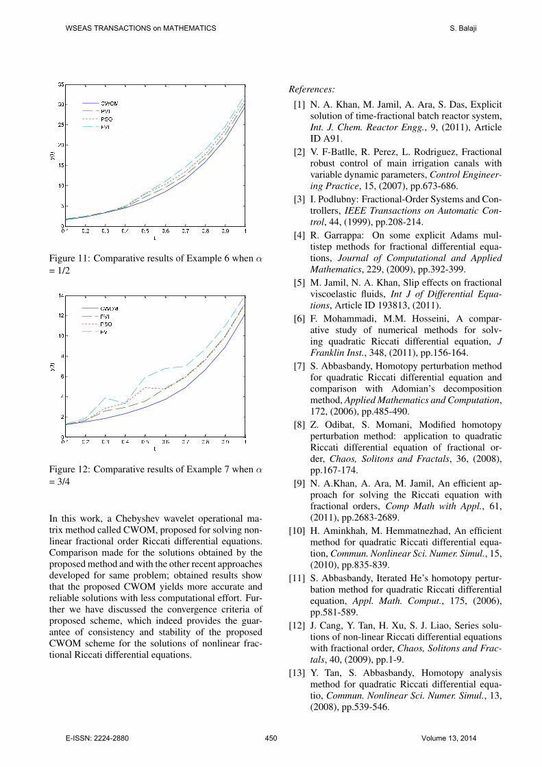
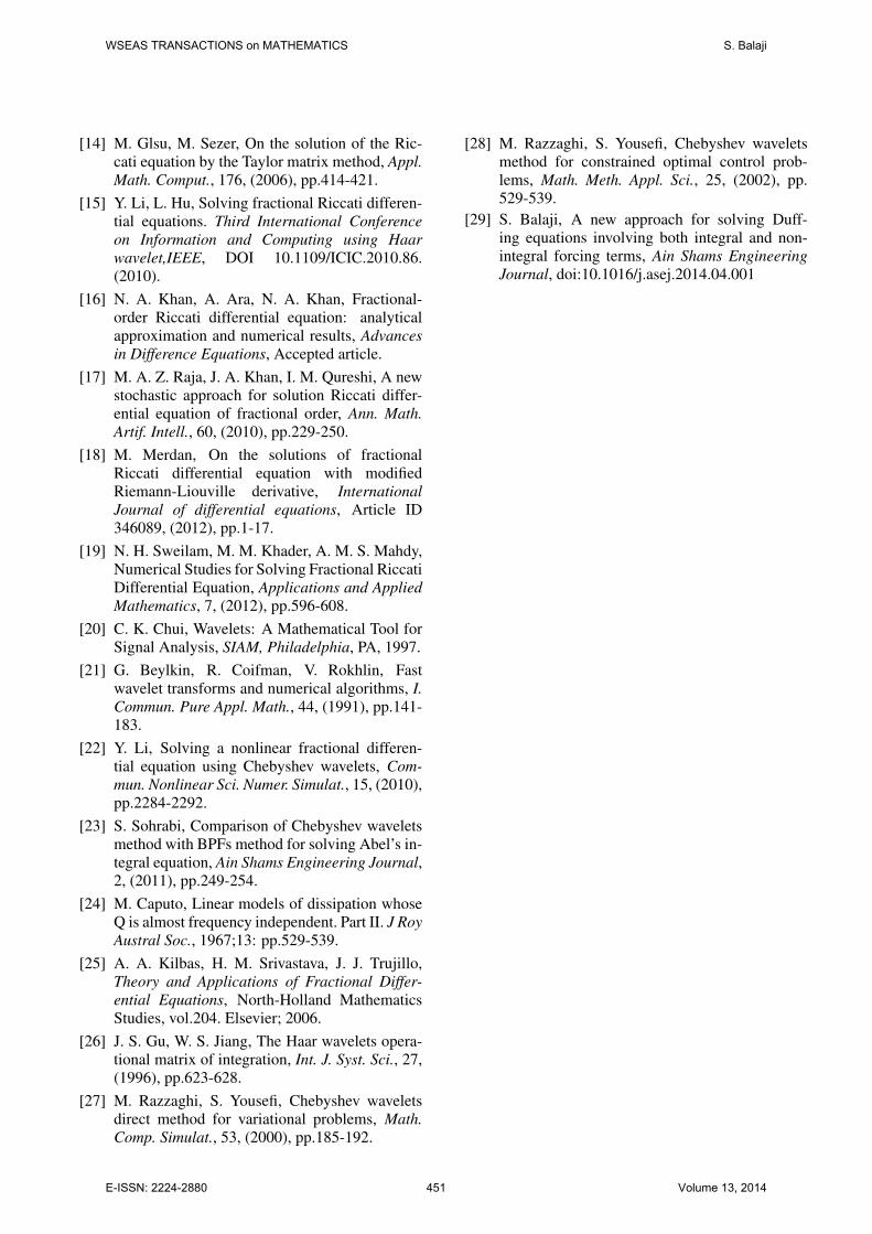
Figure 11: Comparative results of Example 6 when α= 1/2
Figure 12: Comparative results of Example 7 when α= 3/4
In this work, a Chebyshev wavelet operational ma-trix method called CWOM, proposed for solving non-linear fractional order Riccati differential equations.Comparison made for the solutions obtained by theproposed method and with the other recent approachesdeveloped for same problem; obtained results showthat the proposed CWOM yields more accurate andreliable solutions with less computational effort. Fur-ther we have discussed the convergence criteria ofproposed scheme, which indeed provides the guar-antee of consistency and stability of the proposedCWOM scheme for the solutions of nonlinear frac-tional Riccati differential equations.
References:
[1] N. A. Khan, M. Jamil, A. Ara, S. Das, Explicitsolution of time-fractional batch reactor system,Int. J. Chem. Reactor Engg., 9, (2011), ArticleID A91.
[2] V. F-Batlle, R. Perez, L. Rodriguez, Fractionalrobust control of main irrigation canals withvariable dynamic parameters, Control Engineer-ing Practice, 15, (2007), pp.673-686.
[3] I. Podlubny: Fractional-Order Systems and Con-trollers, IEEE Transactions on Automatic Con-trol, 44, (1999), pp.208-214.
[4] R. Garrappa: On some explicit Adams mul-tistep methods for fractional differential equa-tions, Journal of Computational and AppliedMathematics, 229, (2009), pp.392-399.
[5] M. Jamil, N. A. Khan, Slip effects on fractionalviscoelastic fluids, Int J of Differential Equa-tions, Article ID 193813, (2011).
[6] F. Mohammadi, M.M. Hosseini, A compar-ative study of numerical methods for solv-ing quadratic Riccati differential equation, JFranklin Inst., 348, (2011), pp.156-164.
[7] S. Abbasbandy, Homotopy perturbation methodfor quadratic Riccati differential equation andcomparison with Adomian’s decompositionmethod, Applied Mathematics and Computation,172, (2006), pp.485-490.
[8] Z. Odibat, S. Momani, Modified homotopyperturbation method: application to quadraticRiccati differential equation of fractional or-der, Chaos, Solitons and Fractals, 36, (2008),pp.167-174.
[9] N. A.Khan, A. Ara, M. Jamil, An efficient ap-proach for solving the Riccati equation withfractional orders, Comp Math with Appl., 61,(2011), pp.2683-2689.
[10] H. Aminkhah, M. Hemmatnezhad, An efficientmethod for quadratic Riccati differential equa-tion, Commun. Nonlinear Sci. Numer. Simul., 15,(2010), pp.835-839.
[11] S. Abbasbandy, Iterated He’s homotopy pertur-bation method for quadratic Riccati differentialequation, Appl. Math. Comput., 175, (2006),pp.581-589.
[12] J. Cang, Y. Tan, H. Xu, S. J. Liao, Series solu-tions of non-linear Riccati differential equationswith fractional order, Chaos, Solitons and Frac-tals, 40, (2009), pp.1-9.
[13] Y. Tan, S. Abbasbandy, Homotopy analysismethod for quadratic Riccati differential equa-tio, Commun. Nonlinear Sci. Numer. Simul., 13,(2008), pp.539-546.
WSEAS TRANSACTIONS on MATHEMATICS S. Balaji
E-ISSN: 2224-2880 450 Volume 13, 2014
[14] M. Glsu, M. Sezer, On the solution of the Ric-cati equation by the Taylor matrix method, Appl.Math. Comput., 176, (2006), pp.414-421.
[15] Y. Li, L. Hu, Solving fractional Riccati differen-tial equations. Third International Conferenceon Information and Computing using Haarwavelet,IEEE, DOI 10.1109/ICIC.2010.86.(2010).
[16] N. A. Khan, A. Ara, N. A. Khan, Fractional-order Riccati differential equation: analyticalapproximation and numerical results, Advancesin Difference Equations, Accepted article.
[17] M. A. Z. Raja, J. A. Khan, I. M. Qureshi, A newstochastic approach for solution Riccati differ-ential equation of fractional order, Ann. Math.Artif. Intell., 60, (2010), pp.229-250.
[18] M. Merdan, On the solutions of fractionalRiccati differential equation with modifiedRiemann-Liouville derivative, InternationalJournal of differential equations, Article ID346089, (2012), pp.1-17.
[19] N. H. Sweilam, M. M. Khader, A. M. S. Mahdy,Numerical Studies for Solving Fractional RiccatiDifferential Equation, Applications and AppliedMathematics, 7, (2012), pp.596-608.
[20] C. K. Chui, Wavelets: A Mathematical Tool forSignal Analysis, SIAM, Philadelphia, PA, 1997.
[21] G. Beylkin, R. Coifman, V. Rokhlin, Fastwavelet transforms and numerical algorithms, I.Commun. Pure Appl. Math., 44, (1991), pp.141-183.
[22] Y. Li, Solving a nonlinear fractional differen-tial equation using Chebyshev wavelets, Com-mun. Nonlinear Sci. Numer. Simulat., 15, (2010),pp.2284-2292.
[23] S. Sohrabi, Comparison of Chebyshev waveletsmethod with BPFs method for solving Abel’s in-tegral equation, Ain Shams Engineering Journal,2, (2011), pp.249-254.
[24] M. Caputo, Linear models of dissipation whoseQ is almost frequency independent. Part II. J RoyAustral Soc., 1967;13: pp.529-539.
[25] A. A. Kilbas, H. M. Srivastava, J. J. Trujillo,Theory and Applications of Fractional Differ-ential Equations, North-Holland MathematicsStudies, vol.204. Elsevier; 2006.
[26] J. S. Gu, W. S. Jiang, The Haar wavelets opera-tional matrix of integration, Int. J. Syst. Sci., 27,(1996), pp.623-628.
[27] M. Razzaghi, S. Yousefi, Chebyshev waveletsdirect method for variational problems, Math.Comp. Simulat., 53, (2000), pp.185-192.
[28] M. Razzaghi, S. Yousefi, Chebyshev waveletsmethod for constrained optimal control prob-lems, Math. Meth. Appl. Sci., 25, (2002), pp.529-539.
[29] S. Balaji, A new approach for solving Duff-ing equations involving both integral and non-integral forcing terms, Ain Shams EngineeringJournal, doi:10.1016/j.asej.2014.04.001
WSEAS TRANSACTIONS on MATHEMATICS S. Balaji
E-ISSN: 2224-2880 451 Volume 13, 2014