Embed Size (px)
Citation preview

EE263 Autumn 2015 S. Boyd and S. Lall
Solution via Laplace transform and matrix exponential
I Laplace transform
I solving x = Ax via Laplace transform
I state transition matrix
I matrix exponential
I qualitative behavior and stability
1

Laplace transform of matrix valued function
suppose z : R+ → Rp×q
Laplace transform: Z = L(z), where Z : D ⊆ C→ Cp×q is defined by
Z(s) =
∫ ∞0
e−stz(t) dt
I integral of matrix is done term-by-term
I convention: upper case denotes Laplace transform
I D is the domain or region of convergence of Z
I D includes at least {s | <s > a}, where a satisfies |zij(t)| ≤ αeat for t ≥ 0,i = 1, . . . , p, j = 1, . . . , q
2

Derivative property
L(z) = sZ(s)− z(0)
to derive, integrate by parts:
L(z)(s) =
∫ ∞0
e−stz(t) dt
= e−stz(t)∣∣t→∞t=0
+ s
∫ ∞0
e−stz(t) dt
= sZ(s)− z(0)
3

Laplace transform solution of x = Ax
consider continuous-time time-invariant (TI) LDS
x = Ax
for t ≥ 0, where x(t) ∈ Rn
I take Laplace transform: sX(s)− x(0) = AX(s)
I rewrite as (sI −A)X(s) = x(0)
I hence X(s) = (sI −A)−1x(0)
I take inverse transform
x(t) = L−1 ((sI −A)−1)x(0)
4

Resolvent and state transition matrix
I (sI −A)−1 is called the resolvent of A
I resolvent defined for s ∈ C except eigenvalues of A, i.e., s such that det(sI−A) = 0
I Φ(t) = L−1((sI −A)−1
)is called the state-transition matrix; it maps the
initial state to the state at time t:
x(t) = Φ(t)x(0)
(in particular, state x(t) is a linear function of initial state x(0))
5

Example 1: Harmonic oscillator
x =
[0 1−1 0
]x
−2 −1.5 −1 −0.5 0 0.5 1 1.5 2−2
−1.5
−1
−0.5
0
0.5
1
1.5
2
6

Example 1: Harmonic oscillator
sI −A =
[s −11 s
], so resolvent is
(sI −A)−1 =
[ ss2+1
1s2+1
−1s2+1
ss2+1
](eigenvalues are ±i)
state transition matrix is
Φ(t) = L−1
([ ss2+1
1s2+1
−1s2+1
ss2+1
])=
[cos t sin t− sin t cos t
]a rotation matrix (−t radians)
so we have x(t) =
[cos t sin t− sin t cos t
]x(0)
7

Example 2: Double integrator
x =
[0 10 0
]x
−2 −1.5 −1 −0.5 0 0.5 1 1.5 2−2
−1.5
−1
−0.5
0
0.5
1
1.5
2
8

Example 2: Double integrator
sI −A =
[s −10 s
], so resolvent is
(sI −A)−1 =
[1s
1s2
0 1s
](eigenvalues are 0, 0)
state transition matrix is
Φ(t) = L−1
([1s
1s2
0 1s
])=
[1 t0 1
]
so we have x(t) =
[1 t0 1
]x(0)
9

Characteristic polynomial
X (s) = det(sI −A) is called the characteristic polynomial of A
I X (s) is a polynomial of degree n, with leading (i.e., sn) coefficient one
I roots of X are the eigenvalues of A
I X has real coefficients, so eigenvalues are either real or occur in conjugatepairs
I there are n eigenvalues (if we count multiplicity as roots of X )
10

Eigenvalues of A and poles of resolvent
i, j entry of resolvent can be expressed via Cramer’s rule as
(−1)i+jdet ∆ij
det(sI −A)
where ∆ij is sI −A with jth row and ith column deleted
I det ∆ij is a polynomial of degree less than n, so i, j entry of resolvent hasform fij(s)/X (s) where fij is polynomial with degree less than n
I poles of entries of resolvent must be eigenvalues of A
I but not all eigenvalues of A show up as poles of each entry
(when there are cancellations between det ∆ij and X (s))
11

Matrix exponential
define matrix exponential as
eM = I +M +M2
2!+ · · ·
I converges for all M ∈ Rn×n
I looks like ordinary power series
eat = 1 + ta+(ta)2
2!+ · · ·
with square matrices instead of scalars . . .
12

Matrix exponential
(I − C)−1 = I + C + C2 + C3 + · · · (if series converges)
I series expansion of resolvent:
(sI −A)−1 = (1/s)(I −A/s)−1 =I
s+A
s2+A2
s3+ · · ·
(valid for |s| large enough) so
Φ(t) = L−1 ((sI −A)−1) = I + tA+(tA)2
2!+ · · ·
I with this definition, state-transition matrix is
Φ(t) = L−1 ((sI −A)−1) = etA
13

Matrix exponential solution of autonomous LDS
solution of x = Ax, with A ∈ Rn×n and constant, is
x(t) = etAx(0)
generalizes scalar case: solution of x = ax, with a ∈ R and constant, is
x(t) = etax(0)
14

Properties of matrix exponential
I matrix exponential is meant to look like scalar exponential
I some things you’d guess hold for the matrix exponential (by analogy with thescalar exponential) do in fact hold
I but many things you’d guess are wrong
example: you might guess that eA+B = eAeB , but it’s false (in general)
A =
[0 1−1 0
], B =
[0 10 0
]eA =
[0.54 0.84−0.84 0.54
], eB =
[1 10 1
]eA+B =
[0.16 1.40−0.70 0.16
]6= eAeB =
[0.54 1.38−0.84 −0.30
]
15

Properties of matrix exponential
eA+B = eAeB if AB = BA
i.e., product rule holds when A and B commute
thus for t, s ∈ R, e(tA+sA) = etAesA
with s = −t we getetAe−tA = etA−tA = e0 = I
so etA is nonsingular, with inverse(etA)−1
= e−tA
16
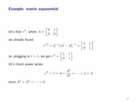
Example: matrix exponential
let’s find eA, where A =
[0 10 0
]we already found
etA = L−1(sI −A)−1 =
[1 t0 1
]so, plugging in t = 1, we get eA =
[1 10 1
]let’s check power series:
eA = I +A+A2
2!+ · · · = I +A
since A2 = A3 = · · · = 0
17

Time transfer property
for x = Ax we knowx(t) = Φ(t)x(0) = etAx(0)
interpretation: the matrix etA propagates initial condition into state at time t
more generally we have, for any t and τ ,
x(τ + t) = etAx(τ)
(to see this, apply result above to z(t) = x(t+ τ))
interpretation: the matrix etA propagates state t seconds forward in time (backwardif t < 0)
18

Time transfer property
I recall first order (forward Euler) approximate state update, for small t:
x(τ + t) ≈ x(τ) + tx(τ) = (I + tA)x(τ)
I exact solution is
x(τ + t) = etAx(τ) = (I + tA+ (tA)2/2! + · · · )x(τ)
I forward Euler is just first two terms in series
19

Sampling a continuous-time system
suppose x = Ax
sample x at times t1 ≤ t2 ≤ · · · : define z(k) = x(tk)
then z(k + 1) = e(tk+1−tk)Az(k)
for uniform sampling tk+1 − tk = h, so
z(k + 1) = ehAz(k),
a discrete-time LDS (called discretized version of continuous-time system)
20

Piecewise constant system
consider time-varying LDS x = A(t)x, with
A(t) =
A0 0 ≤ t < t1A1 t1 ≤ t < t2...
where 0 < t1 < t2 < · · · (sometimes called jump linear system)
for t ∈ [ti, ti+1] we have
x(t) = e(t−ti)Ai · · · e(t3−t2)A2e(t2−t1)A1et1A0x(0)
(matrix on righthand side is called state transition matrix for system, and denotedΦ(t))
21

Qualitative behavior of x(t)
suppose x = Ax, x(t) ∈ Rn
then x(t) = etAx(0); X(s) = (sI −A)−1x(0)
ith component Xi(s) has form
Xi(s) =ai(s)
X (s)
where ai is a polynomial of degree < n
thus the poles of Xi are all eigenvalues of A (but not necessarily the other wayaround)
22
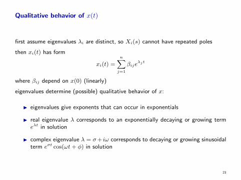
Qualitative behavior of x(t)
first assume eigenvalues λi are distinct, so Xi(s) cannot have repeated poles
then xi(t) has form
xi(t) =
n∑j=1
βijeλjt
where βij depend on x(0) (linearly)
eigenvalues determine (possible) qualitative behavior of x:
I eigenvalues give exponents that can occur in exponentials
I real eigenvalue λ corresponds to an exponentially decaying or growing termeλt in solution
I complex eigenvalue λ = σ+ iω corresponds to decaying or growing sinusoidalterm eσt cos(ωt+ φ) in solution
23

Qualitative behavior of x(t)
I <λj gives exponential growth rate (if > 0), or exponential decay rate (if < 0)of term
I =λj gives frequency of oscillatory term (if 6= 0)
ℜs
ℑseigenvalues
24

Repeated eigenvalues
now suppose A has repeated eigenvalues, so Xi can have repeated poles
express eigenvalues as λ1, . . . , λr (distinct) with multiplicities n1, . . . , nr, respec-tively (n1 + · · ·+ nr = n)
then xi(t) has form
xi(t) =
r∑j=1
pij(t)eλjt
where pij(t) is a polynomial of degree < nj (that depends linearly on x(0))
25

Stability
we say system x = Ax is stable if etA → 0 as t→∞
meaning:
I state x(t) converges to 0, as t→∞, no matter what x(0) is
I all trajectories of x = Ax converge to 0 as t→∞
fact: x = Ax is stable if and only if all eigenvalues of A have negative real part:
<λi < 0, i = 1, . . . , n
26

Stability
the ‘if’ part is clear sincelimt→∞
p(t)eλt = 0
for any polynomial, if <λ < 0
we’ll see the ‘only if’ part next lecture
more generally, maxi <λi determines the maximum asymptotic logarithmic growthrate of x(t) (or decay, if < 0)
27