Embed Size (px)
Citation preview

Solutions Manual
Hadi SaadatProfessor of Electrical EngineeringMilwaukee School of Engineering
Milwaukee, Wisconsin
McGraw-Hill, Inc.

CONTENTS
1 THE POWER SYSTEM: AN OVERVIEW 1
2 BASIC PRINCIPLES 5
3 GENERATOR AND TRANSFORMER MODELS;THE PER-UNIT SYSTEM 25
4 TRANSMISSION LINE PARAMETERS 52
5 LINE MODEL AND PERFORMANCE 68
6 POWER FLOW ANALYSIS 107
7 OPTIMAL DISPATCH OF GENERATION 147
8 SYNCHRONOUS MACHINE TRANSIENT ANALYSIS 170
9 BALANCED FAULT 181
10 SYMMETRICAL COMPONENTS AND UNBALANCED FAULT 208
11 STABILITY 244
12 POWER SYSTEM CONTROL 263
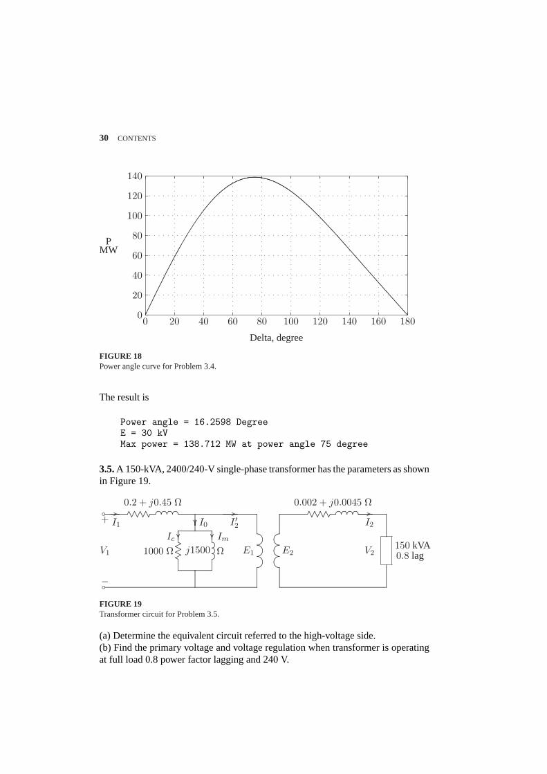
i

CHAPTER 1 PROBLEMS
1.1 The demand estimation is the starting point for planning the future electricpower supply. The consistency of demand growth over the years has led to numer-ous attempts to fit mathematical curves to this trend. One of the simplest curvesis
P = P0ea(t−t0)
wherea is the average per unit growth rate,P is the demand in yeart, andP0 isthe given demand at yeart0.
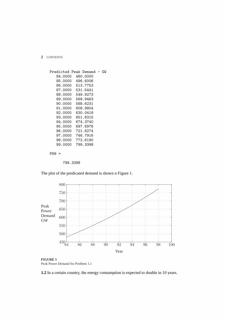
Assume the peak power demand in the United States in 1984 is 480 GW withan average growth rate of 3.4 percent. UsingMATLAB, plot the predicated peakdemand in GW from 1984 to 1999. Estimate the peak power demand for the year1999.We use the following commands to plot the demand growth
t0 = 84; P0 = 480;a =.034;t =(84:1:99)’;P =P0*exp(a*(t-t0));disp(’Predicted Peak Demand - GW’)disp([t, P])plot(t, P), gridxlabel(’Year’), ylabel(’Peak power demand GW’)P99 =P0*exp(a*(99 - t0))
The result is
1
2 CONTENTS
Predicted Peak Demand - GW84.0000 480.000085.0000 496.600686.0000 513.775387.0000 531.544188.0000 549.927389.0000 568.946390.0000 588.623191.0000 608.980492.0000 630.041893.0000 651.831594.0000 674.374095.0000 697.697896.0000 721.827497.0000 746.791698.0000 772.619099.0000 799.3398
P99 =
799.3398
The plot of the predicated demand is shown n Figure 1.
450
500
550
600
650
700
750
800
PeakPowerDemandGW
84 86 88 90 92 94 96 98 100
Year
........................................
.........................................
.......................................
.......................................
.....................................
....................................
.....................................
....................................
...................................
..................................
..................................
.................................
................................
................................
................................
...............................
...............................
..............................
..............................
............................
.......
.
.
.
.
.
.
.
.
.
.
.
.
.
.
.
.
.
.
.
.
.
.
.
.
.
.
.
.
.
.
.
.
.
.
.
.
.
.
.
.
.
.
.
.
.
.
.
.
.
.
.
.
.
.
.
.
.
.
.
.
.
.
.
.
.
.
.
.
.
.
.
.
.
.
.
.
.
.
.
.
.
.
.
.
.
.
.
.
.
.
.
.
.
.
.
.
.
.
.
.
.
.
.
.
.
.
.
.
.
.
.
.
.
.
.
.
.
.
.
.
.
.
.
.
.
.
.
.
.
.
.
.
.
.
.
.
.
.
.
.
.
.
.
.
.
.
.
.
.
.
.
.
.
.
.
.
.
.
.
.
.
.
.
.
.
.
.
.
.
.
.
.
.
.
.
.
.
.
.
.
.
.
.
.
.
.
.
.
.
.
.
.
.
.
.
.
.
.
.
.
.
.
.
.
.
.
.
.
.
.
.
.
.
.
.
.
.
.
.
.
.
.
.
.
.
.
.
.
.
.
.
.
.
.
.
.
.
.
.
.
.
.
.
.
.
.
.
.
. . . . . . . . . . . . . . . . . . . . . . . . . . . . . . . . . . . . . . . . . . . . . . . . . . . . . . . .
. . . . . . . . . . . . . . . . . . . . . . . . . . . . . . . . . . . . . . . . . . . . . . . . . . . . . . . .
. . . . . . . . . . . . . . . . . . . . . . . . . . . . . . . . . . . . . . . . . . . . . . . . . . . . . . . .
. . . . . . . . . . . . . . . . . . . . . . . . . . . . . . . . . . . . . . . . . . . . . . . . . . . . . . . .
. . . . . . . . . . . . . . . . . . . . . . . . . . . . . . . . . . . . . . . . . . . . . . . . . . . . . . . .
. . . . . . . . . . . . . . . . . . . . . . . . . . . . . . . . . . . . . . . . . . . . . . . . . . . . . . . .
. . . . . . . . . . . . . . . . . . . . . . . . . . . . . . . . . . . . . . . . . . . . . . . . . . . . . . . .
. . . . . . . . . . . . . . . . . . . . . . . . . . . . . . . . . . . . . . . . . . . . . . . . . . . . . . . .
FIGURE 1Peak Power Demand for Problem 1.1
1.2 In a certain country, the energy consumption is expected to double in 10 years.
CONTENTS 3
Assuming a simple exponential growth given by
P = P0eat
calculate the growth ratea.
2P0 = P0e10a
ln 2 = 10a
Solving fora, we have
a =0.69310
= 0.0693 = 6.93%
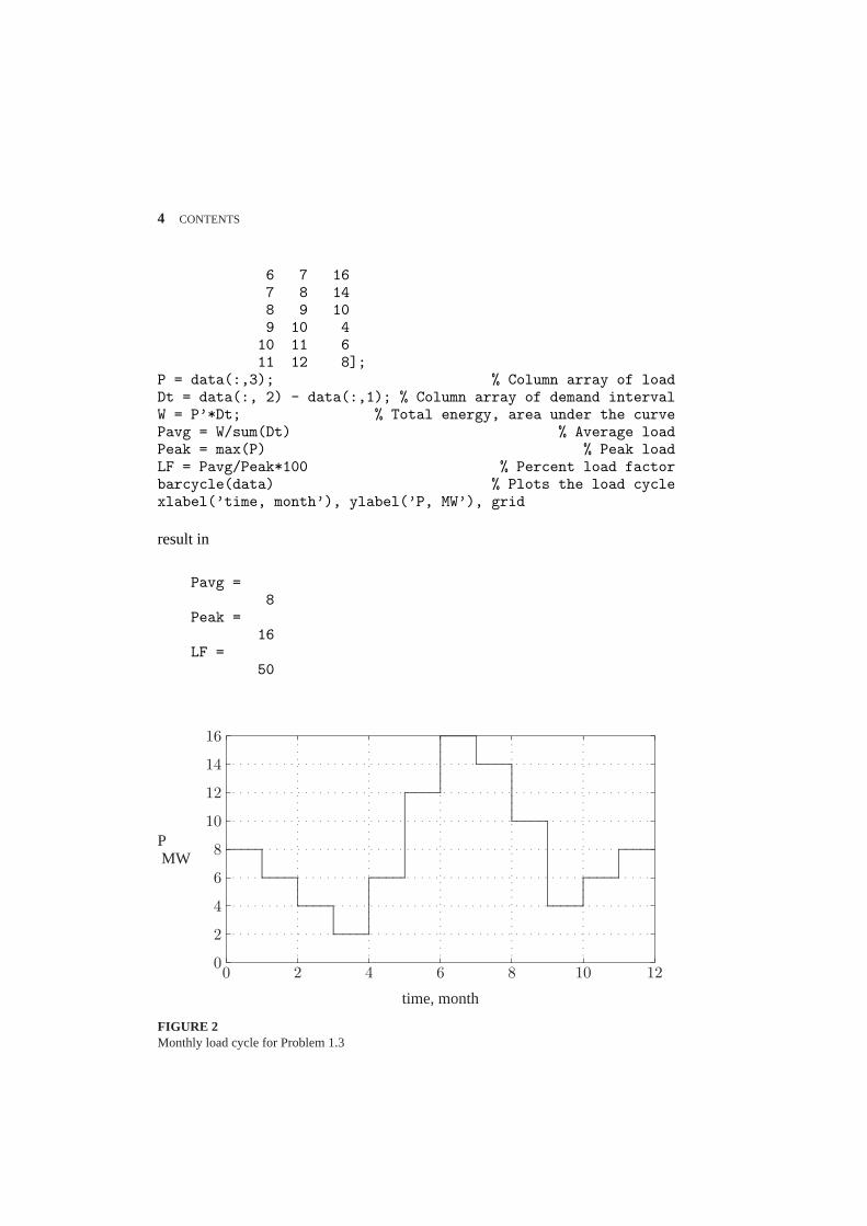
1.3. The annual load of a substation is given in the following table. During eachmonth, the power is assumed constant at an average value. UsingMATLABandthebarcycle function, obtain a plot of the annual load curve. Write the necessarystatements to find the average load and the annual load factor.
Annual System LoadInterval – Month Load – MWJanuary 8February 6March 4April 2May 6June 12July 16August 14September 10October 4November 6December 8
The following commands
data = [ 0 1 81 2 62 3 43 4 24 5 65 6 12
4 CONTENTS
6 7 167 8 148 9 109 10 410 11 611 12 8];
P = data(:,3); % Column array of loadDt = data(:, 2) - data(:,1); % Column array of demand intervalW = P’*Dt; % Total energy, area under the curvePavg = W/sum(Dt) % Average loadPeak = max(P) % Peak loadLF = Pavg/Peak*100 % Percent load factorbarcycle(data) % Plots the load cyclexlabel(’time, month’), ylabel(’P, MW’), grid
result in
Pavg =8
Peak =16
LF =50
0
2
4
6
8
10
12
14
16
PMW
0 2 4 6 8 10 12
time, month
..................................................................................................................................................................................................................................................................................................................................................................................................................................................................................................................................................................................
........
........
........
........
........
........
........
........
........
........
........
........
........
........
........
........
........
..........................................................................................................................................................................................................................................................................................................................................................................................................................................................................................................................................................................................................................................................................................................................................
........
........
........
........
........
..............................................................................................................................................................................
.
.
.
.
.
.
.
.
.
.
.
.
.
.
.
.
.
.
.
.
.
.
.
.
.
.
.
.
.
.
.
.
.
.
.
.
.
.
.
.
.
.
.
.
.
.
.
.
.
.
.
.
.
.
.
.
.
.
.
.
.
.
.
.
.
.
.
.
.
.
.
.
.
.
.
.
.
.
.
.
.
.
.
.
.
.
.
.
.
.
.
.
.
.
.
.
.
.
.
.
.
.
.
.
.
.
.
.
.
.
.
.
.
.
.
.
.
.
.
.
.
.
.
.
.
.
.
.
.
.
.
.
.
.
.
.
.
.
.
.
.
.
.
.
.
.
.
.
.
.
.
.
.
.
.
.
.
.
.
.
. . . . . . . . . . . . . . . . . . . . . . . . . . . . . . . . . . . . . . . . . . . . . . . . . . . . . . . . . . .
. . . . . . . . . . . . . . . . . . . . . . . . . . . . . . . . . . . . . . . . . . . . . . . . . . . . . . . . . . .
. . . . . . . . . . . . . . . . . . . . . . . . . . . . . . . . . . . . . . . . . . . . . . . . . . . . . . . . . . .
. . . . . . . . . . . . . . . . . . . . . . . . . . . . . . . . . . . . . . . . . . . . . . . . . . . . . . . . . . .
. . . . . . . . . . . . . . . . . . . . . . . . . . . . . . . . . . . . . . . . . . . . . . . . . . . . . . . . . . .
. . . . . . . . . . . . . . . . . . . . . . . . . . . . . . . . . . . . . . . . . . . . . . . . . . . . . . . . . . .
. . . . . . . . . . . . . . . . . . . . . . . . . . . . . . . . . . . . . . . . . . . . . . . . . . . . . . . . . . .
FIGURE 2Monthly load cycle for Problem 1.3

CHAPTER 2 PROBLEMS
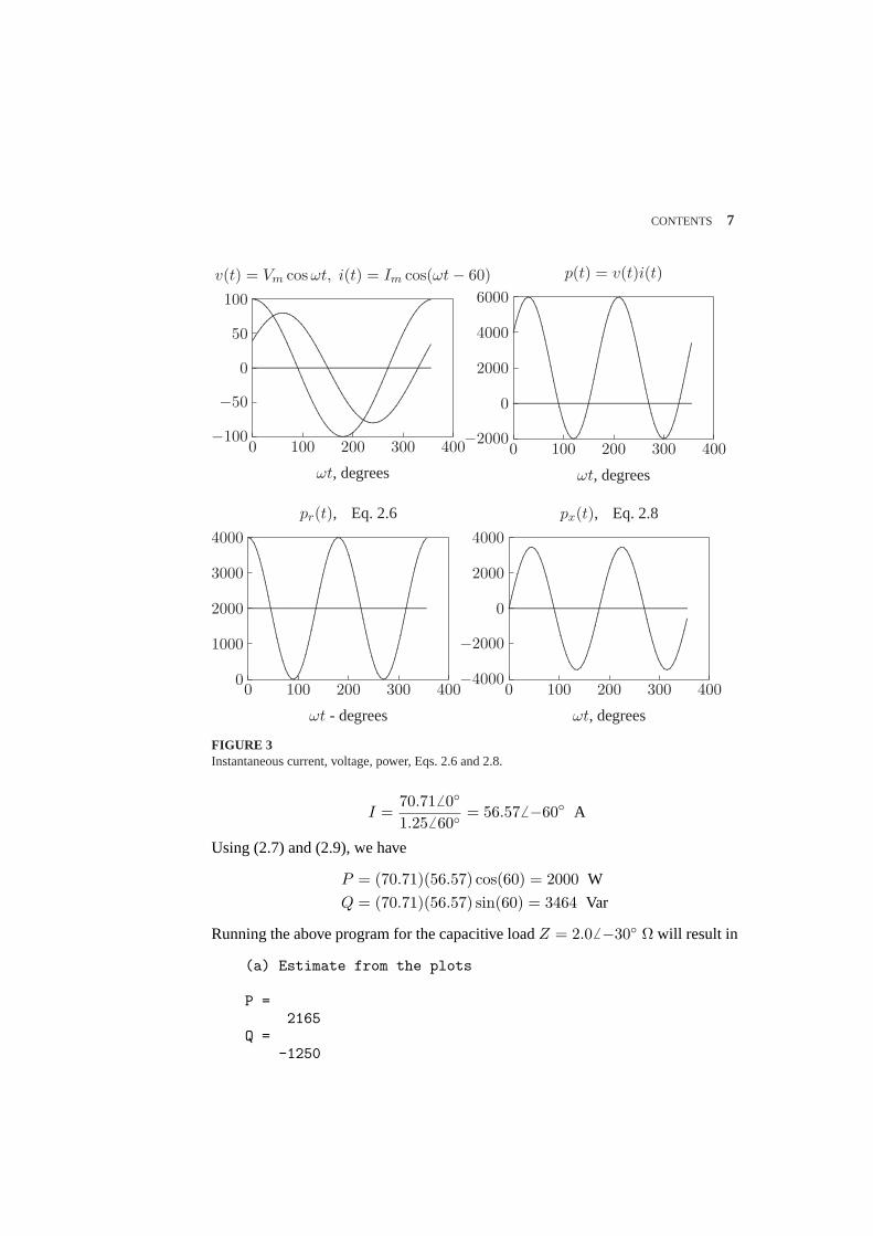
2.1.Modify the program in Example 2.1 such that the following quantities can beentered by the user:The peak amplitudeVm, and the phase angleθv of the sinusoidal supplyv(t) =Vm cos(ωt + θv). The impedance magnitudeZ, and its phase angleγ of the load.The program should produce plots fori(t), v(t), p(t), pr(t) andpx(t), similar toExample 2.1. Run the program forVm = 100 V, θv = 0 and the following loads:
An inductive load,Z = 1.256 60 ΩA capacitive load,Z = 2.06 −30 ΩA resistive load, Z = 2.56 0 Ω
(a) Frompr(t) andpx(t) plots, estimate the real and reactive power for each load.Draw a conclusion regarding the sign of reactive power for inductive and capaci-tive loads.(b) Using phasor values of current and voltage, calculate the real and reactive powerfor each load and compare with the results obtained from the curves.(c) If the above loads are all connected across the same power supply, determinethe total real and reactive power taken from the supply.
The following statements are used to plot the instantaneous voltage, current, andthe instantaneous terms given by(2-6) and (2-8).
Vm = input(’Enter voltage peak amplitude Vm = ’);thetav =input(’Enter voltage phase angle in degree thetav = ’);Vm = 100; thetav = 0; % Voltage amplitude and phase angleZ = input(’Enter magnitude of the load impedance Z = ’);gama = input(’Enter load phase angle in degree gama = ’);thetai = thetav - gama; % Current phase angle in degree
5

6 CONTENTS
theta = (thetav - thetai)*pi/180; % Degree to radianIm = Vm/Z; % Current amplitudewt=0:.05:2*pi; % wt from 0 to 2*piv=Vm*cos(wt); % Instantaneous voltagei=Im*cos(wt + thetai*pi/180); % Instantaneous currentp=v.*i; % Instantaneous powerV=Vm/sqrt(2); I=Im/sqrt(2); % RMS voltage and currentpr = V*I*cos(theta)*(1 + cos(2*wt)); % Eq. (2.6)px = V*I*sin(theta)*sin(2*wt); % Eq. (2.8)disp(’(a) Estimate from the plots’)P = max(pr)/2, Q = V*I*sin(theta)*sin(2*pi/4)P = P*ones(1, length(wt)); % Average power for plotxline = zeros(1, length(wt)); % generates a zero vectorwt=180/pi*wt; % converting radian to degreesubplot(221), plot(wt, v, wt, i,wt, xline), gridtitle([’v(t)=Vm coswt, i(t)=Im cos(wt +’,num2str(thetai),’)’])xlabel(’wt, degrees’)subplot(222), plot(wt, p, wt, xline), gridtitle(’p(t)=v(t) i(t)’), xlabel(’wt, degrees’)subplot(223), plot(wt, pr, wt, P, wt,xline), gridtitle(’pr(t) Eq. 2.6’), xlabel(’wt, degrees’)subplot(224), plot(wt, px, wt, xline), gridtitle(’px(t) Eq. 2.8’), xlabel(’wt, degrees’)subplot(111)disp(’(b) From P and Q formulas using phasor values ’)P=V*I*cos(theta) % Average powerQ = V*I*sin(theta) % Reactive power
The result for the inductive loadZ = 1.256 60Ω is
Enter voltage peak amplitude Vm = 100Enter voltage phase angle in degree thatav = 0Enter magnitude of the load impedance Z = 1.25Enter load phase angle in degree gama = 60
(a) Estimate from the plots
P =2000
Q =3464
(b) For the inductive loadZ = 1.256 60Ω, the rms values of voltage and currentare
V =1006 0
1.414= 70.716 0 V
CONTENTS 7
−100
−50
0
50
100
0 100 200 300 400
ωt, degrees
v(t) = Vm cosωt, i(t) = Im cos(ωt− 60)
.................................................................................................................................................................................................................................................................................................................
................................................................................................................................................................................................................................................................................................................................................................................................................................................................................................................................................................................................................................
.................................................................................................................................................................................................................................................................................................................................................................................
...............................................................................................................................................................
−2000
0
2000
4000
6000
0 100 200 300 400
ωt, degrees
p(t) = v(t)i(t)
.................................................................................................................................................................................................................................................................................................................
...............................................................................................................................................................................................................................................................................................................................................................
........................................................................................................................................................................................................................................................................................................................................................................................................................................................................................................................................................
.....................................................................................................................................................................
0
1000
2000
3000
4000
0 100 200 300 400
ωt - degrees
pr(t), Eq. 2.6
.................................................................................................................................................................................................................................................................................................................
..............................................................................................................................................................................................................................................................................................................................................................................................................................................................................................................................................................................................................................................................................................................................................................................................................................................
.........................................................................................................................................................................................................................................................
−4000
−2000
0
2000
4000
0 100 200 300 400
ωt, degrees
px(t), Eq. 2.8
................................................................................................................................................................................................................................................................................................................................................................................................................................................................................................................................................................................................................................................................................................
..........................................................................................................................................................................................................................................................................................................................................................................................................................................................................................
.......................................................................................
FIGURE 3Instantaneous current, voltage, power, Eqs. 2.6 and 2.8.
I =70.716 0
1.256 60= 56.576 −60 A
Using (2.7) and (2.9), we have
P = (70.71)(56.57) cos(60) = 2000 W
Q = (70.71)(56.57) sin(60) = 3464 Var
Running the above program for the capacitive loadZ = 2.0 6 −30 Ω will result in
(a) Estimate from the plots
P =2165
Q =-1250
8 CONTENTS
Similarly, for Z = 2.56 0 Ω, we get
P =2000
Q =0
(c) With the above three loads connected in parallel across the supply, the total realand reactive powers are
P = 2000 + 2165 + 2000 = 6165 W
Q = 3464− 1250 + 0 = 2214 Var
2.2.A single-phase load is supplied with a sinusoidal voltage
v(t) = 200 cos(377t)
The resulting instantaneous power is
p(t) = 800 + 1000 cos(754t− 36.87)
(a) Find the complex power supplied to the load.(b) Find the instantaneous currenti(t) and the rms value of the current supplied tothe load.(c) Find the load impedance.(d) UseMATLABto plotv(t), p(t), andi(t) = p(t)/v(t) over a range of0 to 16.67ms in steps of 0.1 ms. From the current plot, estimate the peak amplitude, phaseangle and the angular frequency of the current, and verify the results obtained inpart (b). Note inMATLABthe command for array or element-by-element divisionis ./.
p(t) = 800 + 1000 cos(754t− 36.87)= 800 + 1000 cos 36.87 cos 754t + sin 36.87 sin 754t= 800 + 800 cos 754t + 600 sin 754t= 800[1 + cos 2(377)t] + 600 sin 2(377)t
p(t) is in the same form as (2.5), thusP = 600 W, andQ = 600, Var, or
S = 800 + j600 = 10006 36.87 VA
(b) UsingS = 12VmIm
∗, we have
10006 36.87 =122006 0Im
CONTENTS 9
or
Im = 10 6 −36.87 A
Therefore, the instantaneous current is
i(t) = 10cos(377t− 36.87) A
(c)
ZL =V
I=
2006 0
106 −36.87= 206 36.87 Ω
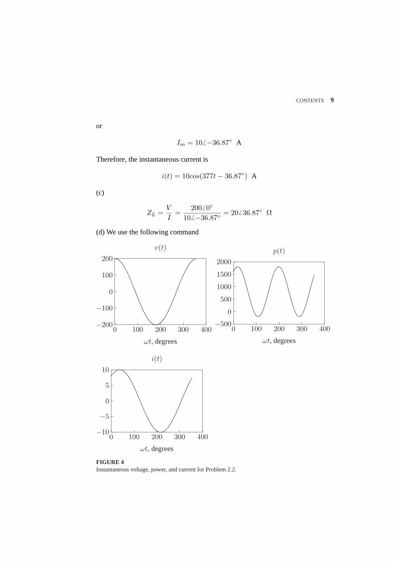
(d) We use the following command
−200
−100
0
100
200
0 100 200 300 400
ωt, degrees
v(t)..............................................................................................................................................................................................................................................................................................................................................................................
..........................................................................................................................................................................................................................................................................................................................
−500
0
500
1000
1500
2000
0 100 200 300 400
ωt, degrees
p(t)
...................................................................................................................................................................................................................................................................................
...........................................................................................................................................................................................................................................................................................................................................................................................................................................................................
..........................................................................................................................................................................
−10
−5
0
5
10
0 100 200 300 400
ωt, degrees
i(t)
................................................................................................................................................................................................................................................................................................................................................................................................................
......................................................................................................................................................................................................................................................
FIGURE 4Instantaneous voltage, power, and current for Problem 2.2.
10 CONTENTS
Vm = 200;t=0:.0001:0.01667; % wt from 0 to 2*piv=Vm*cos(377*t); % Instantaneous voltagep = 800 + 1000*cos(754*t - 36.87*pi/180);% Instantaneous poweri=p./v; % Instantaneous currentwt=180/pi*377*t; % converting radian to degreexline = zeros(1, length(wt)); % generates a zero vectorsubplot(221), plot(wt, v, wt, xline), gridxlabel(’wt, degrees’), title(’v(t)’)subplot(222), plot(wt, p, wt, xline), gridxlabel(’wt, degrees’), title(’p(t)’)subplot(223), plot(wt, i, wt, xline), gridxlabel(’wt, degrees’), title(’i(t)’), subplot(111)
The result is shown in Figure 4. The inspection of current plot shows that the peakamplitude of the current is10 A, lagging voltage by36.87, with an angular fre-quency of 377 Rad/sec.
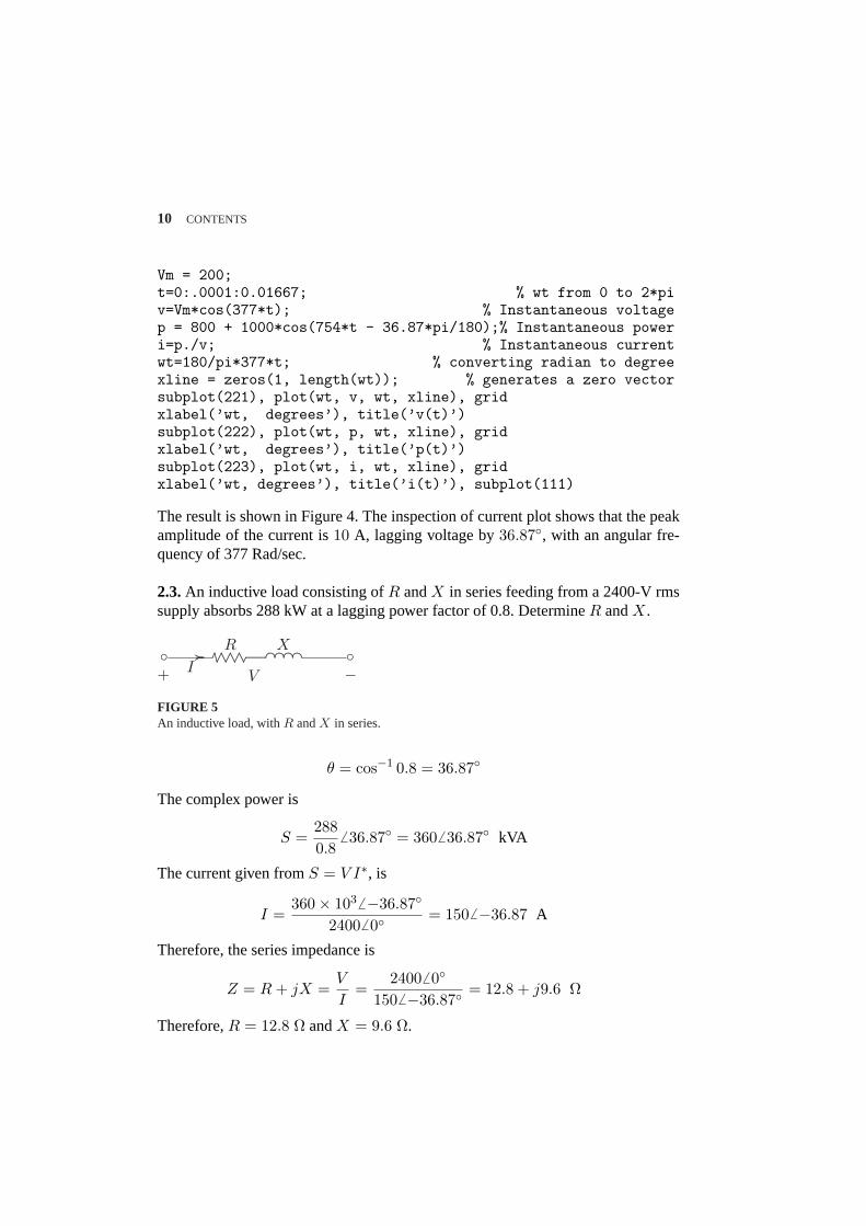
2.3.An inductive load consisting ofR andX in series feeding from a 2400-V rmssupply absorbs 288 kW at a lagging power factor of 0.8. DetermineR andX.
......................................................................
.......................................................................
.................................... ......................... ...........
.............. ......................... ............
......................................... ................
VI
R X
+ −
FIGURE 5An inductive load, withR andX in series.
θ = cos−1 0.8 = 36.87
The complex power is
S =2880.8
6 36.87 = 3606 36.87 kVA
The current given fromS = V I∗, is
I =360× 103 6 −36.87
24006 0= 1506 −36.87 A
Therefore, the series impedance is
Z = R + jX =V
I=
24006 0
1506 −36.87= 12.8 + j9.6 Ω
Therefore,R = 12.8 Ω andX = 9.6 Ω.
CONTENTS 11
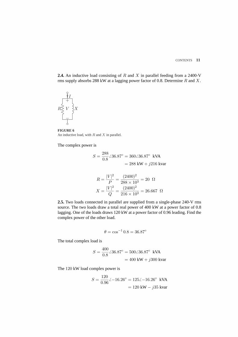
2.4. An inductive load consisting ofR andX in parallel feeding from a 2400-Vrms supply absorbs 288 kW at a lagging power factor of 0.8. DetermineR andX.
.........................................................................................................................................................................................................................................................................................................................................
..............................................................
..........................................................................................................................................................................
................................
........
........
........
V
I
R X
+
−
FIGURE 6An inductive load, withR andX in parallel.
The complex power is
S =2880.8
6 36.87 = 360 6 36.87 kVA
= 288 kW + j216 kvar
R =|V |2P
=(2400)2
288× 103= 20 Ω
X =|V |2Q
=(2400)2
216× 103= 26.667 Ω
2.5.Two loads connected in parallel are supplied from a single-phase 240-V rmssource. The two loads draw a total real power of 400 kW at a power factor of 0.8lagging. One of the loads draws 120 kW at a power factor of 0.96 leading. Find thecomplex power of the other load.
θ = cos−1 0.8 = 36.87
The total complex load is
S =4000.8
6 36.87 = 500 6 36.87 kVA
= 400 kW + j300 kvar
The120 kW load complex power is
S =1200.96
6 −16.26 = 1256 −16.26 kVA
= 120 kW− j35 kvar
12 CONTENTS
Therefore, the second load complex power is
S2 = 400 + j300− (120− j35) = 280 kW + j335 kvar
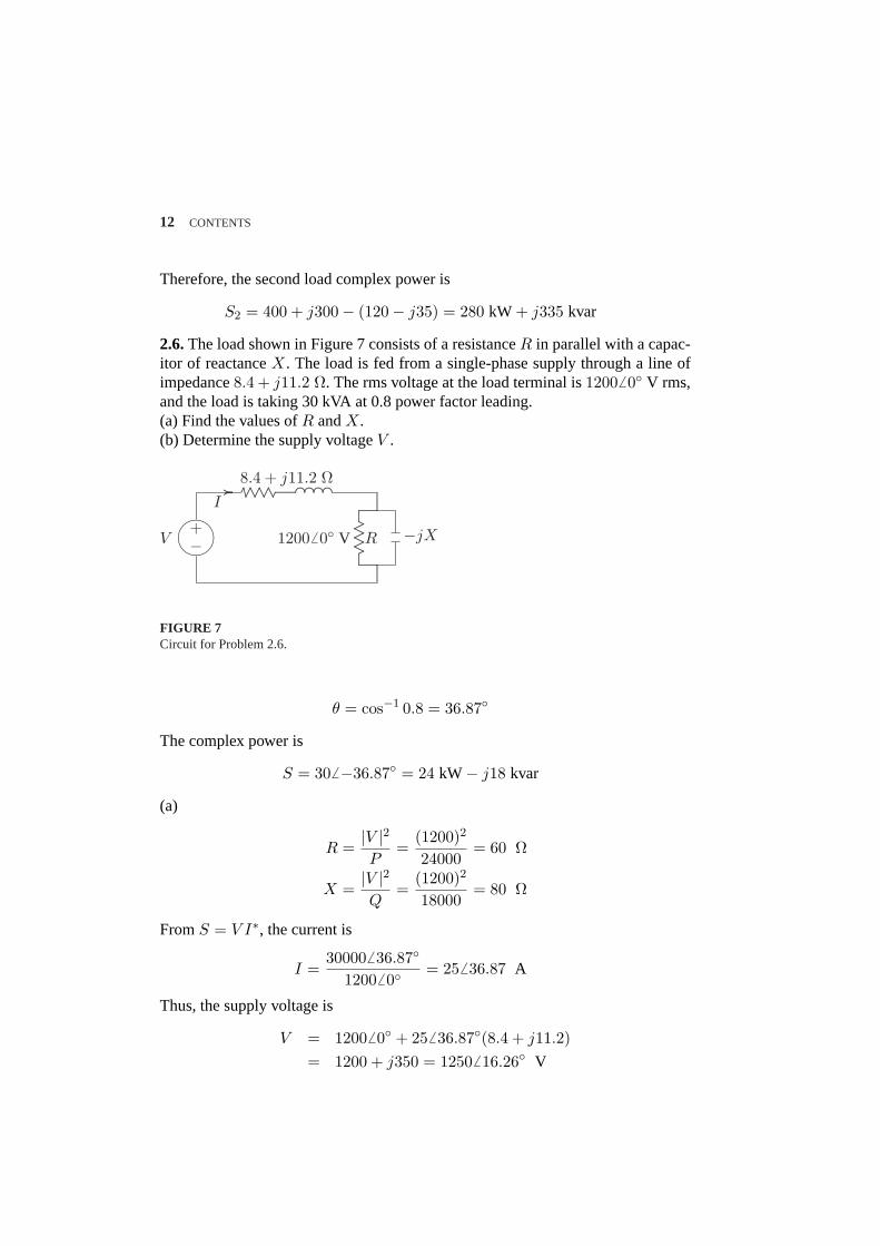
2.6.The load shown in Figure 7 consists of a resistanceR in parallel with a capac-itor of reactanceX. The load is fed from a single-phase supply through a line ofimpedance8.4 + j11.2 Ω. The rms voltage at the load terminal is12006 0 V rms,and the load is taking 30 kVA at 0.8 power factor leading.(a) Find the values ofR andX.(b) Determine the supply voltageV .
¹¸
º·......................................................................
.......................................................................
.................................... ......................... ...........
.............. ......................... ............
............. ..................................................................................................................................................................................................................................................................................................
............................ ................
V
I
8.4 + j11.2 Ω
R −jX12006 0 V+−
FIGURE 7Circuit for Problem 2.6.
θ = cos−1 0.8 = 36.87
The complex power is
S = 306 −36.87 = 24 kW− j18 kvar
(a)
R =|V |2P
=(1200)2
24000= 60 Ω
X =|V |2Q
=(1200)2
18000= 80 Ω
FromS = V I∗, the current is
I =300006 36.87
12006 0= 256 36.87 A
Thus, the supply voltage is
V = 12006 0 + 25 6 36.87(8.4 + j11.2)= 1200 + j350 = 12506 16.26 V
CONTENTS 13
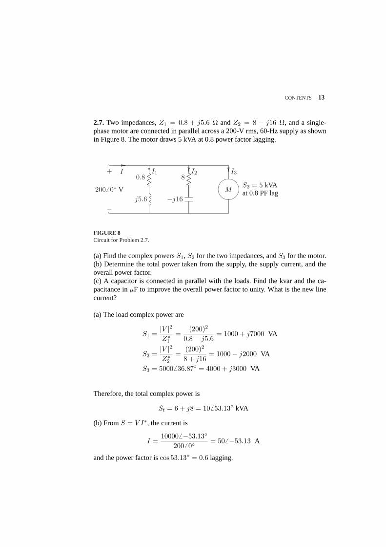
2.7. Two impedances,Z1 = 0.8 + j5.6 Ω andZ2 = 8 − j16 Ω, and a single-phase motor are connected in parallel across a 200-V rms, 60-Hz supply as shownin Figure 8. The motor draws 5 kVA at 0.8 power factor lagging.
........
........
........
............................................................................................................................................................
....................................
......................................................
........
........
........
........
........
.............................................................................
........
........
........
........
.......
........
........
........
........
........
...............................................
....................................
...............................................................
ÁÀ
¿................................ ................
........................
........
........
........ ................................................ ........................
........
........
........
I I1 I2 I3
2006 0 V
0.8
j5.6
8
−j16
S3 = 5 kVAat 0.8 PF lagM
+
−a
a
FIGURE 8Circuit for Problem 2.7.
(a) Find the complex powersS1, S2 for the two impedances, andS3 for the motor.(b) Determine the total power taken from the supply, the supply current, and theoverall power factor.(c) A capacitor is connected in parallel with the loads. Find the kvar and the ca-pacitance inµF to improve the overall power factor to unity. What is the new linecurrent?
(a) The load complex power are
S1 =|V |2Z∗1
=(200)2
0.8− j5.6= 1000 + j7000 VA
S2 =|V |2Z∗2
=(200)2
8 + j16= 1000− j2000 VA
S3 = 50006 36.87 = 4000 + j3000 VA
Therefore, the total complex power is
St = 6 + j8 = 106 53.13 kVA
(b) FromS = V I∗, the current is
I =100006 −53.13
2006 0= 506 −53.13 A
and the power factor iscos 53.13 = 0.6 lagging.
14 CONTENTS
(c) For overall unity power factor,QC = 8000 Var, and the capacitive impedanceis
ZC =|V |2SC
∗ =(200)2
j8000= −j5 Ω
and the capacitance is
C =106
(2π)(60)(5)= 530.5 µF
The new current is
I =60006 0
2006 0= 30 6 0 A
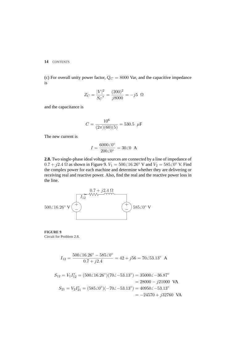
2.8.Two single-phase ideal voltage sources are connected by a line of impedance of0.7 + j2.4 Ω as shown in Figure 9.V1 = 5006 16.26 V andV2 = 5856 0 V. Findthe complex power for each machine and determine whether they are delivering orreceiving real and reactive power. Also, find the real and the reactive power loss inthe line.
¹¸
º·......................................................................
.......................................................................
.................................... ......................... ...........
.............. ......................... ...........
..............
¹¸
º·............................ ................
5006 16.26 V
I12
0.7 + j2.4 Ω
5856 0 V+−
+−
FIGURE 9Circuit for Problem 2.8.
I12 =5006 16.26 − 5856 0
0.7 + j2.4= 42 + j56 = 706 53.13 A
S12 = V1I∗12 = (5006 16.26)(706 −53.13) = 350006 −36.87
= 28000− j21000 VA
S21 = V2I∗21 = (5856 0)(−706 −53.13) = 409506 −53.13
= −24570 + j32760 VA
CONTENTS 15
From the above results, sinceP1 is positive andP2 is negative, source 1 generates28 kW, and source 2 receives24.57 kW, and the real power loss is3.43 kW. Sim-ilarly, sinceQ1 is negative, source 1 receives21 kvar and source 2 delivers32.76kvar. The reactive power loss in the line is11.76 kvar.
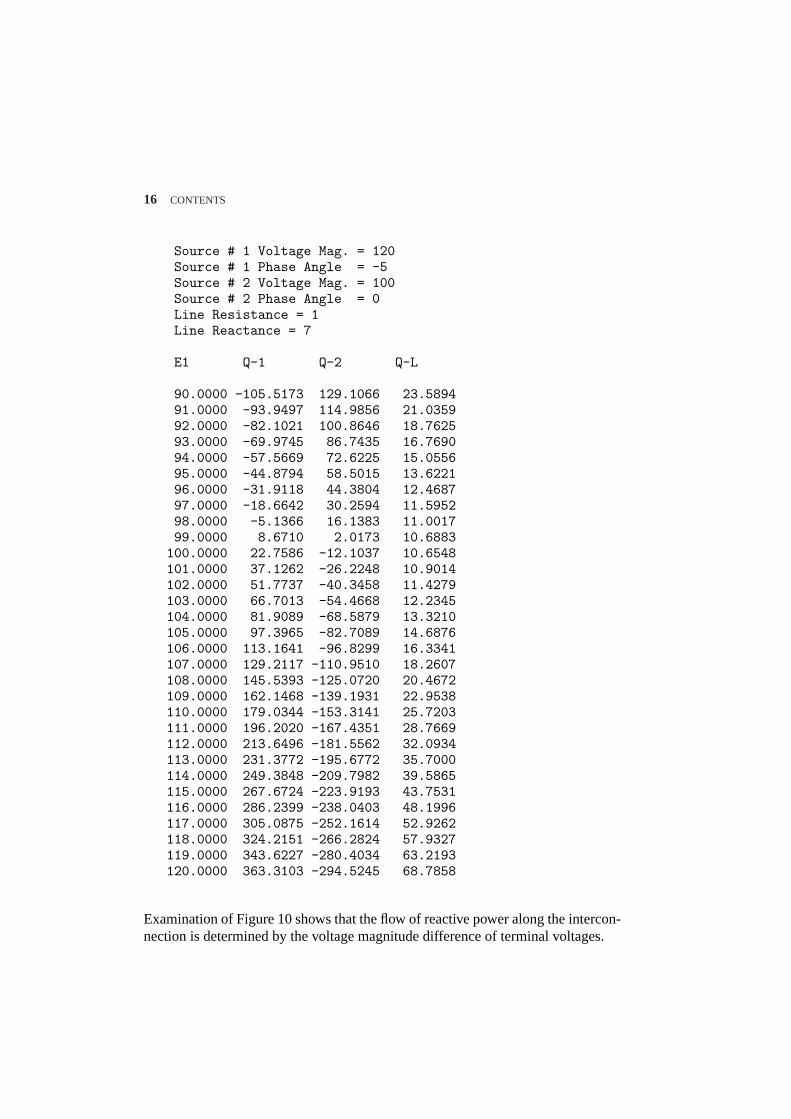
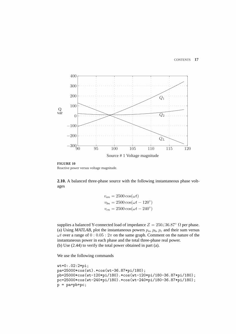
2.9.Write aMATLABprogram for the system of Example 2.5 such that the voltagemagnitude of source 1 is changed from 75 percent to 100 percent of the given valuein steps of 1 volt. The voltage magnitude of source 2 and the phase angles of thetwo sources is to be kept constant. Compute the complex power for each source andthe line loss. Tabulate the reactive powers and plotQ1, Q2, andQL versus voltagemagnitude|V1|. From the results, show that the flow of reactive power along theinterconnection is determined by the magnitude difference of the terminal voltages.
We use the following commands
E1 = input(’Source # 1 Voltage Mag. = ’);a1 = input(’Source # 1 Phase Angle = ’);E2 = input(’Source # 2 Voltage Mag. = ’);a2 = input(’Source # 2 Phase Angle = ’);R = input(’Line Resistance = ’);X = input(’Line Reactance = ’);Z = R + j*X; % Line impedanceE1 = (0.75*E1:1:E1)’; % Change E1 form 75% to 100% E1a1r = a1*pi/180; % Convert degree to radiank = length(E1);E2 = ones(k,1)*E2;%create col. Array of same length for E2a2r = a2*pi/180; % Convert degree to radianV1=E1.*cos(a1r) + j*E1.*sin(a1r);V2=E2.*cos(a2r) + j*E2.*sin(a2r);I12 = (V1 - V2)./Z; I21=-I12;S1= V1.*conj(I12); P1 = real(S1); Q1 = imag(S1);S2= V2.*conj(I21); P2 = real(S2); Q2 = imag(S2);SL= S1+S2; PL = real(SL); QL = imag(SL);Result1=[E1, Q1, Q2, QL];disp(’ E1 Q-1 Q-2 Q-L ’)disp(Result1)plot(E1, Q1, E1, Q2, E1, QL), gridxlabel(’ Source #1 Voltage Magnitude’)ylabel(’ Q, var’)text(112.5, -180, ’Q2’)text(112.5, 5,’QL’), text(112.5, 197, ’Q1’)
The result is
16 CONTENTS
Source # 1 Voltage Mag. = 120Source # 1 Phase Angle = -5Source # 2 Voltage Mag. = 100Source # 2 Phase Angle = 0Line Resistance = 1Line Reactance = 7
E1 Q-1 Q-2 Q-L
90.0000 -105.5173 129.1066 23.589491.0000 -93.9497 114.9856 21.035992.0000 -82.1021 100.8646 18.762593.0000 -69.9745 86.7435 16.769094.0000 -57.5669 72.6225 15.055695.0000 -44.8794 58.5015 13.622196.0000 -31.9118 44.3804 12.468797.0000 -18.6642 30.2594 11.595298.0000 -5.1366 16.1383 11.001799.0000 8.6710 2.0173 10.6883100.0000 22.7586 -12.1037 10.6548101.0000 37.1262 -26.2248 10.9014102.0000 51.7737 -40.3458 11.4279103.0000 66.7013 -54.4668 12.2345104.0000 81.9089 -68.5879 13.3210105.0000 97.3965 -82.7089 14.6876106.0000 113.1641 -96.8299 16.3341107.0000 129.2117 -110.9510 18.2607108.0000 145.5393 -125.0720 20.4672109.0000 162.1468 -139.1931 22.9538110.0000 179.0344 -153.3141 25.7203111.0000 196.2020 -167.4351 28.7669112.0000 213.6496 -181.5562 32.0934113.0000 231.3772 -195.6772 35.7000114.0000 249.3848 -209.7982 39.5865115.0000 267.6724 -223.9193 43.7531116.0000 286.2399 -238.0403 48.1996117.0000 305.0875 -252.1614 52.9262118.0000 324.2151 -266.2824 57.9327119.0000 343.6227 -280.4034 63.2193120.0000 363.3103 -294.5245 68.7858
Examination of Figure 10 shows that the flow of reactive power along the intercon-nection is determined by the voltage magnitude difference of terminal voltages.
CONTENTS 17
−300
−200
−100
0
100
200
300
400
Qvar
90 95 100 105 110 115 120
Source # 1 Voltage magnitude
....................................................
..................................................
...............................................
..............................................
.............................................
...........................................
.........................................
..........................................
..........................................
.......................................
.......................................
.....................................
......................................
...................................
...................................
....................................
...................................
...................................
.......
.....................................................................................................................................................................................................................................................................................................................................................................................................................................................................................................................................................................................................................................................................................................................................................
.................................................................................................................................................................................................................................................................................................................................................................................................................................................................................................................................................................
....................................................................................................................................
...................
Q1
Q2
QL
.
.
.
.
.
.
.
.
.
.
.
.
.
.
.
.
.
.
.
.
.
.
.
.
.
.
.
.
.
.
.
.
.
.
.
.
.
.
.
.
.
.
.
.
.
.
.
.
.
.
.
.
.
.
.
.
.
.
.
.
.
.
.
.
.
.
.
.
.
.
.
.
.
.
.
.
.
.
.
.
.
.
.
.
.
.
.
.
.
.
.
.
.
.
.
.
.
.
.
.
.
.
.
.
.
.
.
.
.
.
.
.
.
.
.
.
.
.
.
.
.
.
.
.
.
.
.
.
.
.
.
.
.
.
.
.
.
.
.
.
.
.
.
.
.
.
.
.
.
.
.
.
.
.
.
.
.
.
.
.
.
.
.
.
.
.
.
.
.
.
.
.
.
.
.
.
.
.
.
.
.
.
.
.
.
.
.
.
.
.
.
.
.
.
.
.
.
.
.
.
.
.
.
.
.
.
.
.
.
.
.
.
.
.
.
.
. . . . . . . . . . . . . . . . . . . . . . . . . . . . . . . . . . . . . . . . . . . . . . . . . . . . . . . .
. . . . . . . . . . . . . . . . . . . . . . . . . . . . . . . . . . . . . . . . . . . . . . . . . . . . . . . .
. . . . . . . . . . . . . . . . . . . . . . . . . . . . . . . . . . . . . . . . . . . . . . . . . . . . . . . .
. . . . . . . . . . . . . . . . . . . . . . . . . . . . . . . . . . . . . . . . . . . . . . . . . . . . . . . .
. . . . . . . . . . . . . . . . . . . . . . . . . . . . . . . . . . . . . . . . . . . . . . . . . . . . . . . .
. . . . . . . . . . . . . . . . . . . . . . . . . . . . . . . . . . . . . . . . . . . . . . . . . . . . . . . .
FIGURE 10Reactive power versus voltage magnitude.
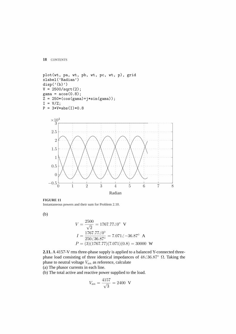
2.10.A balanced three-phase source with the following instantaneous phase volt-ages
van = 2500 cos(ωt)vbn = 2500 cos(ωt− 120)vcn = 2500 cos(ωt− 240)
supplies a balanced Y-connected load of impedanceZ = 2506 36.87 Ω per phase.(a) UsingMATLAB, plot the instantaneous powerspa, pb, pc and their sum versusωt over a range of0 : 0.05 : 2π on the same graph. Comment on the nature of theinstantaneous power in each phase and the total three-phase real power.(b) Use (2.44) to verify the total power obtained in part (a).
We use the following commands
wt=0:.02:2*pi;pa=25000*cos(wt).*cos(wt-36.87*pi/180);pb=25000*cos(wt-120*pi/180).*cos(wt-120*pi/180-36.87*pi/180);pc=25000*cos(wt-240*pi/180).*cos(wt-240*pi/180-36.87*pi/180);p = pa+pb+pc;
18 CONTENTS
plot(wt, pa, wt, pb, wt, pc, wt, p), gridxlabel(’Radian’)disp(’(b)’)V = 2500/sqrt(2);gama = acos(0.8);Z = 250*(cos(gama)+j*sin(gama));I = V/Z;P = 3*V*abs(I)*0.8
−0.5
0
0.5
1
1.5
2
2.5
3
0 1 2 3 4 5 6 7 8
Radian
...........................................................................................................................................................................................................................................................................................................................................................................................................
..........................................................................................................................................................................................................................................................................................................................................................................................................................................................................................................................................................................................................................................................................................
....................................................................................................................................................................................................................................................................
...............................................................................................................................................................................................................................................................................................................................................................................................................................................................................................................................
..........................................................................................................................................................................................................................................................................................................................................................................................................................................................................................................................................................................................................................................................................................................................................................................................................................................
..................................................................................................................................................................................................................................................................................................................................................................................................................................................................................................................................................................................................................................................................................
..........................................................................................................................................................................................................................................................................................................................................................................................................................................................................................................................................................................................................................................................................................
........................................................................................................................................................................................................................................................................................................................................................................................................................................................................................................................................................................................×104
.
.
.
.
.
.
.
.
.
.
.
.
.
.
.
.
.
.
.
.
.
.
.
.
.
.
.
.
.
.
.
.
.
.
.
.
.
.
.
.
.
.
.
.
.
.
.
.
.
.
.
.
.
.
.
.
.
.
.
.
.
.
.
.
.
.
.
.
.
.
.
.
.
.
.
.
.
.
.
.
.
.
.
.
.
.
.
.
.
.
.
.
.
.
.
.
.
.
.
.
.
.
.
.
.
.
.
.
.
.
.
.
.
.
.
.
.
.
.
.
.
.
.
.
.
.
.
.
.
.
.
.
.
.
.
.
.
.
.
.
.
.
.
.
.
.
.
.
.
.
.
.
.
.
.
.
.
.
.
.
.
.
.
.
.
.
.
.
.
.
.
.
.
.
.
.
.
.
.
.
.
.
.
.
.
.
.
.
.
.
.
.
.
.
.
.
.
.
.
.
.
.
.
.
.
.
.
.
.
.
.
.
.
.
.
.
.
. . . . . . . . . . . . . . . . . . . . . . . . . . . . . . . . . . . . . . . . . . . . . . . . . . . . . . . . . .
. . . . . . . . . . . . . . . . . . . . . . . . . . . . . . . . . . . . . . . . . . . . . . . . . . . . . . . . . .
. . . . . . . . . . . . . . . . . . . . . . . . . . . . . . . . . . . . . . . . . . . . . . . . . . . . . . . . . .
. . . . . . . . . . . . . . . . . . . . . . . . . . . . . . . . . . . . . . . . . . . . . . . . . . . . . . . . . .
. . . . . . . . . . . . . . . . . . . . . . . . . . . . . . . . . . . . . . . . . . . . . . . . . . . . . . . . . .
. . . . . . . . . . . . . . . . . . . . . . . . . . . . . . . . . . . . . . . . . . . . . . . . . . . . . . . . . .
. . . . . . . . . . . . . . . . . . . . . . . . . . . . . . . . . . . . . . . . . . . . . . . . . . . . . . . . . .
FIGURE 11Instantaneous powers and their sum for Problem 2.10.
(b)
V =2500√
2= 1767.776 0 V
I =1767.776 0
2506 36.87= 7.0716 −36.87 A
P = (3)(1767.77)(7.071)(0.8) = 30000 W
2.11.A 4157-V rms three-phase supply is applied to a balanced Y-connected three-phase load consisting of three identical impedances of48 6 36.87 Ω. Taking thephase to neutral voltageVan as reference, calculate(a) The phasor currents in each line.(b) The total active and reactive power supplied to the load.
Van =4157√
3= 2400 V
CONTENTS 19
With Van as reference, the phase voltages are:
Van = 24006 0 V Vbn = 24006 −120 V Van = 24006 −240 V
(a) The phasor currents are:
Ia =Van
Z=
24006 0
486 36.87= 506 −36.87 A
Ib =Vbn
Z=
24006 −120
486 36.87= 506 −156.87 A
Ic =Vcn
Z=
24006 −240
486 36.87= 50 6 −276.87 A
(b) The total complex power is
S = 3VanI∗a = (3)(24006 0)(506 36.87) = 3606 36.87 kVA
= 288 kW + j216 KVAR
2.12.Repeat Problem 2.11 with the same three-phase impedances arranged in a∆connection. TakeVab as reference.
Van =4157√
3= 2400 V
With Vab as reference, the phase voltages are:
Iab =Vab
Z=
41576 0
486 36.87= 86.66 −36.87 A
Ia =√
36 −30Iab = (√
36 −30)(86.66 −36.87 = 1506 −66.87 A
For positive phase sequence, current in other lines are
Ib = 1506 −186.87 A, andIc = 1506 53.13 A
(b) The total complex power is
S = 3VabI∗ab = (3)(41576 0)(86.6 6 36.87) = 10806 36.87 kVA
= 864 kW + j648 kvar
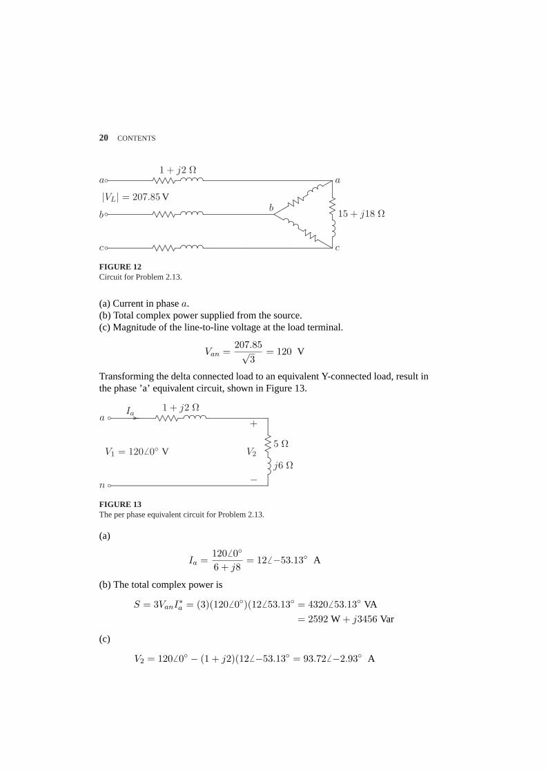
2.13.A balanced delta connected load of15 + j18 Ω per phase is connected at theend of a three-phase line as shown in Figure 12. The line impedance is1+j2 Ω perphase. The line is supplied from a three-phase source with a line-to-line voltage of207.85 V rms. TakingVan as reference, determine the following:
20 CONTENTS
...................................................................................................................................................................................................
.......................................................................
................. ......................... ...........
.............. ......................... ...........
.............. ..................................................................................................................................................................................................................................................................................................................................................................
...................................................................................................................................................................................................
.......................................................................
................. ......................... ...........
.............. ......................... ...........
.............. ..................................................................................................................................................................................................
...................................................................................................................................................................................................
.......................................................................
................. ......................... ...........
.............. ......................... ...........
.............. ..................................................................................................................................................................................................................................................................................................................................................................
...........................................................................................................................................................................
.......................
.........................
.........................
..
........
........
........
.......
................................
..................................................
........
................................................................
.................
.........................................................................
..............................
.
.............................................................................................
..............................................................................
........
.................................................
................................................
1 + j2 Ω
15 + j18 Ω
|VL| = 207.85 V
b
b
b
a
b
c
a
b
c
FIGURE 12Circuit for Problem 2.13.
(a) Current in phasea.(b) Total complex power supplied from the source.(c) Magnitude of the line-to-line voltage at the load terminal.
Van =207.85√
3= 120 V
Transforming the delta connected load to an equivalent Y-connected load, result inthe phase ’a’ equivalent circuit, shown in Figure 13.
...................................................................................................................................................................................................
.......................................................................
................. ......................... ...........
.............. ......................... ...........
.............. .........................................................................................................................................................................
........
........
........
.......
.........................
.........................
.........................
........
.........
..........................................................................................................................................................
...............................................................................................................................................................................................................................................................................................................................................................................................................................................
1 + j2 Ω
5 Ω
j6 ΩV1 = 1206 0 V V2
+
−
b
b
a
n
................................ ................Ia
FIGURE 13The per phase equivalent circuit for Problem 2.13.
(a)
Ia =1206 0
6 + j8= 12 6 −53.13 A
(b) The total complex power is
S = 3VanI∗a = (3)(1206 0)(126 53.13 = 43206 53.13 VA
= 2592 W + j3456 Var
(c)
V2 = 1206 0 − (1 + j2)(126 −53.13 = 93.72 6 −2.93 A
CONTENTS 21
Thus, the magnitude of the line-to-line voltage at the load terminal isVL =√
3(93.72) =162.3 V.
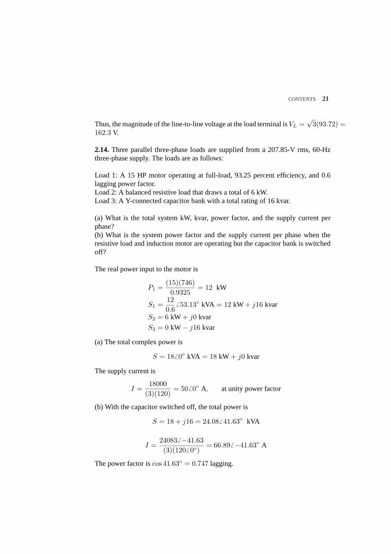
2.14.Three parallel three-phase loads are supplied from a 207.85-V rms, 60-Hzthree-phase supply. The loads are as follows:
Load 1: A 15 HP motor operating at full-load, 93.25 percent efficiency, and 0.6lagging power factor.Load 2: A balanced resistive load that draws a total of 6 kW.Load 3: A Y-connected capacitor bank with a total rating of 16 kvar.
(a) What is the total system kW, kvar, power factor, and the supply current perphase?(b) What is the system power factor and the supply current per phase when theresistive load and induction motor are operating but the capacitor bank is switchedoff?
The real power input to the motor is
P1 =(15)(746)0.9325
= 12 kW
S1 =120.6
6 53.13 kVA = 12 kW + j16 kvar
S2 = 6 kW + j0 kvar
S3 = 0 kW− j16 kvar
(a) The total complex power is
S = 18 6 0 kVA = 18 kW + j0 kvar
The supply current is
I =18000
(3)(120)= 506 0 A, at unity power factor
(b) With the capacitor switched off, the total power is
S = 18 + j16 = 24.086 41.63 kVA
I =240836 −41.63(3)(1206 0)
= 66.89 6 −41.63 A
The power factor iscos 41.63 = 0.747 lagging.
22 CONTENTS
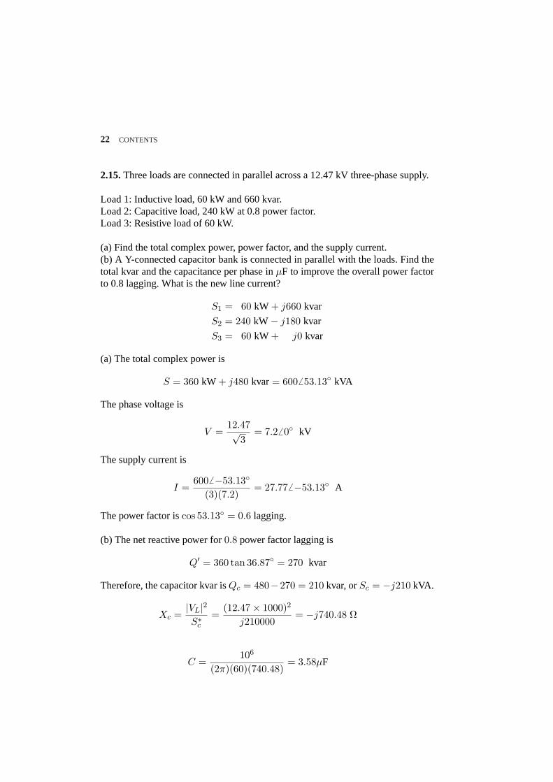
2.15.Three loads are connected in parallel across a 12.47 kV three-phase supply.
Load 1: Inductive load, 60 kW and 660 kvar.Load 2: Capacitive load, 240 kW at 0.8 power factor.Load 3: Resistive load of 60 kW.
(a) Find the total complex power, power factor, and the supply current.(b) A Y-connected capacitor bank is connected in parallel with the loads. Find thetotal kvar and the capacitance per phase inµF to improve the overall power factorto 0.8 lagging. What is the new line current?
S1 = 60 kW + j660 kvar
S2 = 240 kW− j180 kvar
S3 = 60 kW + j0 kvar
(a) The total complex power is
S = 360 kW + j480 kvar = 6006 53.13 kVA
The phase voltage is
V =12.47√
3= 7.26 0 kV
The supply current is
I =6006 −53.13
(3)(7.2)= 27.776 −53.13 A
The power factor iscos 53.13 = 0.6 lagging.
(b) The net reactive power for0.8 power factor lagging is
Q′ = 360 tan 36.87 = 270 kvar
Therefore, the capacitor kvar isQc = 480−270 = 210 kvar, orSc = −j210 kVA.
Xc =|VL|2S∗c
=(12.47× 1000)2
j210000= −j740.48 Ω
C =106
(2π)(60)(740.48)= 3.58µF
CONTENTS 23
.................................................................................................................................... ................................................................................................................................................................................................................................................
................................................................................................................................................................................
............................................................................
........
........
........
........
........
........
........
........
........
........
........
........
........
.......................
................
........
........
........
........
........
........
........
........
....................
................ Q
Q′
P
Qc
θ′ ........................................
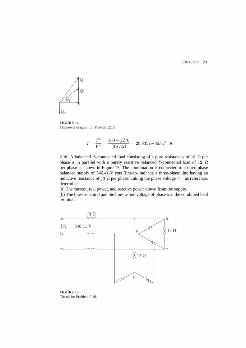
FIGURE 14The power diagram for Problem 2.15.
I =S∗
V ∗ =360− j270
(3)(7.2)= 20.8356 −36.87 A
2.16.A balanced∆-connected load consisting of a pure resistances of18 Ω perphase is in parallel with a purely resistive balanced Y-connected load of12 Ωper phase as shown in Figure 15. The combination is connected to a three-phasebalanced supply of 346.41-V rms (line-to-line) via a three-phase line having aninductive reactance ofj3 Ω per phase. Taking the phase voltageVan as reference,determine(a) The current, real power, and reactive power drawn from the supply.(b) The line-to-neutral and the line-to-line voltage of phasea at the combined loadterminals.
....................................
..................................................
..............
....................................
..................................................
..............
....................................
..................................................
..............
.........................................................................................................................................................................................
............................................................................................................................................................................................................................................................................................................
................................................................................................................................................................................................................
........................................................................................................................................................................................................................................................
................................
..................................................
........
................................................................
...............................
.................................
..............................
..........................................................................................................................................................................
..............................................................................
...................................................
........
................................................................
.................................
................................
............................................................................................................................................
....................................
.......................................
..........................................................................................................................................................
...............................................
j3 Ω
18 Ω
12 Ω
n
|VL| = 346.41 V
b
b
b
a
b
c
a
a
a
a
b
c
FIGURE 15Circuit for Problem 2.16.
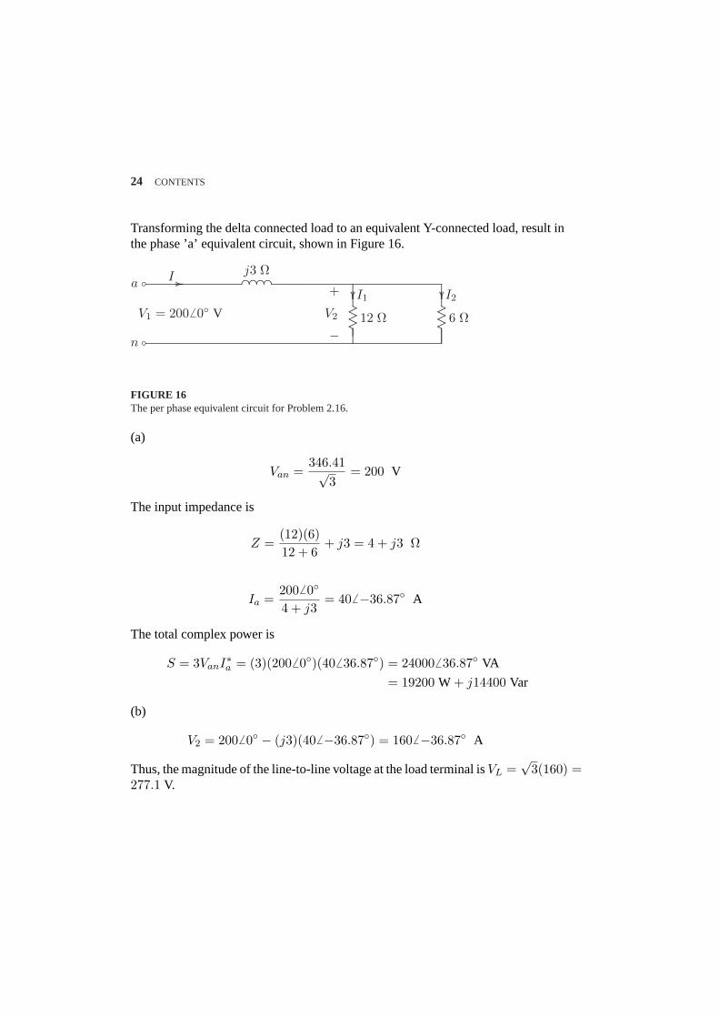
24 CONTENTS
Transforming the delta connected load to an equivalent Y-connected load, result inthe phase ’a’ equivalent circuit, shown in Figure 16.
........................................................................................................................................................................................................ ......................... ...........
.............. ......................... ...........
.............. ...........................................................................................................................................................................................................................................................................................................................................................................................................................................................................................................................................................................................
........
........
........
.......
........
.........
..........................................................................................................................................................
.......................................................................................................................................................................................................................................................................................................................................................................................................................................................................................................................................................................................................................................
j3 Ω
6 Ω12 ΩV1 = 2006 0 V V2
+
−
b
b
a
n
................................ ................
........................
........
........
........ ................................................
I
I1 I2
FIGURE 16The per phase equivalent circuit for Problem 2.16.
(a)
Van =346.41√
3= 200 V
The input impedance is
Z =(12)(6)12 + 6
+ j3 = 4 + j3 Ω
Ia =2006 0
4 + j3= 40 6 −36.87 A
The total complex power is
S = 3VanI∗a = (3)(2006 0)(406 36.87) = 240006 36.87 VA
= 19200 W + j14400 Var
(b)
V2 = 2006 0 − (j3)(406 −36.87) = 1606 −36.87 A
Thus, the magnitude of the line-to-line voltage at the load terminal isVL =√
3(160) =277.1 V.
CHAPTER 3 PROBLEMS
3.1. A three-phase, 318.75-kVA, 2300-V alternator has an armature resistance of0.35Ω/phase and a synchronous reactance of 1.2Ω/phase. Determine the no-loadline-to-line generated voltage and the voltage regulation at(a) Full-load kVA, 0.8 power factor lagging, and rated voltage.(b) Full-load kVA, 0.6 power factor leading, and rated voltage.
Vφ =2300√
3= 1327.9 V
(a) For318.75 kVA, 0.8 power factor lagging,S = 3187506 36.87 VA.
Ia =S∗
3V ∗φ
=3187506 −36.87
(3)(1327.9)= 80 6 −36.87 A
Eφ = 1327.9 + (0.35 + j1.2)(806 −36.87) = 1409.26 2.44 V
The magnitude of the no-load generated voltage isELL =
√3 1409.2 = 2440.8 V, and the voltage regulation is
V.R. =2440.8− 2300
2300× 100 = 6.12%
(b) For318.75 kVA, 0.6 power factor leading,S = 3187506 −53.13 VA.
Ia =S∗
3V ∗φ
=3187506 53.13
(3)(1327.9= 80 6 53.13 A
25
26 CONTENTS
Eφ = 1327.9 + (0.35 + j1.2)(806 53.13) = 1270.46 3.61 V
The magnitude of the no-load generated voltage isELL =
√3 1270.4 = 2220.4 V, and the voltage regulation is
V.R. =2200.4− 2300
2300× 100 = −4.33%
3.2. A 60-MVA, 69.3-kV, three-phase synchronous generator has a synchronousreactance of 15Ω/phase and negligible armature resistance.
(a) The generator is delivering rated power at 0.8 power factor lagging at the ratedterminal voltage to an infinite bus bar. Determine the magnitude of the generatedemf per phase and the power angleδ.
(b) If the generated emf is 36 kV per phase, what is the maximum three-phasepower that the generator can deliver before losing its synchronism?
(c) The generator is delivering 48 MW to the bus bar at the rated voltage withits field current adjusted for a generated emf of 46 kV per phase. Determine thearmature current and the power factor. State whether power factor is lagging orleading?
Vφ =69.3√
3= 40 kV
(a) For60 kVA, 0.8 power factor lagging,S = 600006 36.87 kVA.
Ia =S∗
3V ∗φ
=600006 −36.87
(3)(40)= 5006 −36.87 A
Eφ = 40 + (j15)(5006 −36.87)× 10−3 = 44.96 7.675 kV
(b)
Pmax =3|E||V |
Xs=
(3)(36)(40)15
= 288 MW
(c) ForP = 48 MW, andE = 46 KV/phase, the power angle is given by
48 =(3)(46)(40)
15sin δ
CONTENTS 27
or
δ = 7.4947
and solving for the armature current fromE = V + jXsIa, we have
Ia =460006 7.4947 − 400006 0
j15= 547.47 6 −43.06 A
The power factor iscos−1 43.06 = 0.7306 lagging.
3.3.A 24,000-kVA, 17.32-kV, Y-connected synchronous generator has a synchronousreactance of 5Ω/phase and negligible armature resistance.
(a) At a certain excitation, the generator delivers rated load, 0.8 power factor lag-ging to an infinite bus bar at a line-to-line voltage of 17.32 kV. Determine theexcitation voltage per phase.
(b) The excitation voltage is maintained at 13.4 KV/phase and the terminal voltageat 10 KV/phase. What is the maximum three-phase real power that the generatorcan develop before pulling out of synchronism?
(c) Determine the armature current for the condition of part (b).
Vφ =17.32√
3= 10 kV
(a) For24000 kVA, 0.8 power factor lagging,S = 240006 36.87 kVA.
Ia =S∗
3V ∗φ
=240006 −36.87
(3)(10)= 8006 −36.87 A
Eφ = 10 + (j5)(8006 −36.87)× 10−3 = 12.8066 14.47 kV
(b)
Pmax =3|E||V |
Xs=
(3)(13.4)(10)5
= 80.4 MW
(c) At maximum power transferδ = 90, and solving for the armature current fromE = V + jXsIa, we have
Ia =134006 90 − 100006 0
j5= 3344 6 36.73 A
28 CONTENTS
The power factor iscos−1 36.73 = 0.7306 leading.
3.4. A 34.64-kV, 60-MVA, three-phase salient-pole synchronous generator has adirect axis reactance of 13.5Ω and a quadrature-axis reactance of 9.333Ω. Thearmature resistance is negligible.
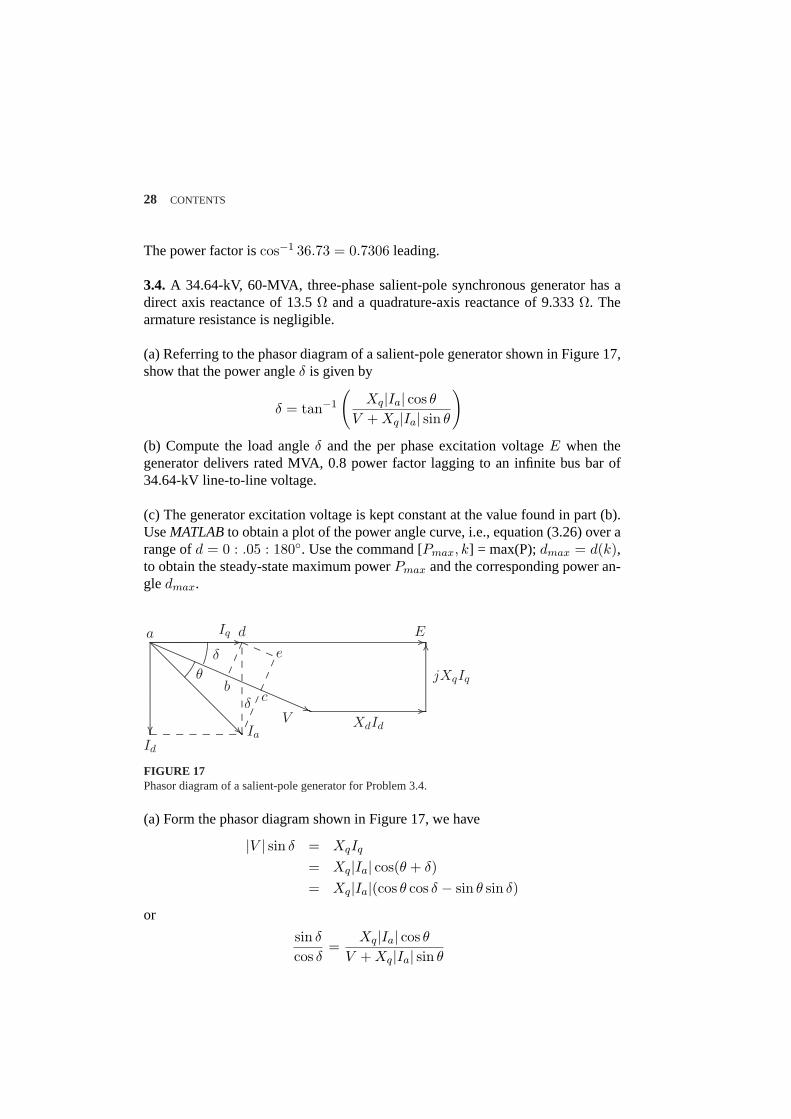
(a) Referring to the phasor diagram of a salient-pole generator shown in Figure 17,show that the power angleδ is given by
δ = tan−1
(Xq|Ia| cos θ
V + Xq|Ia| sin θ
)
(b) Compute the load angleδ and the per phase excitation voltageE when thegenerator delivers rated MVA, 0.8 power factor lagging to an infinite bus bar of34.64-kV line-to-line voltage.
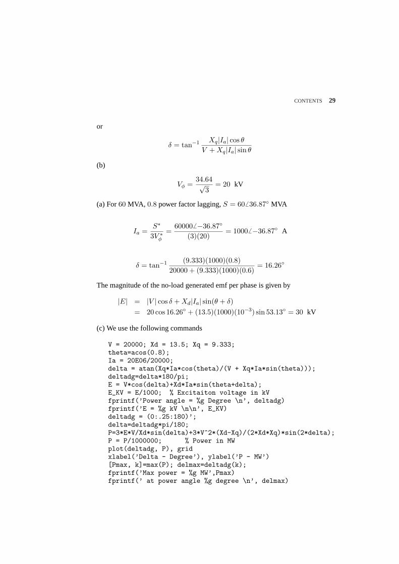
(c) The generator excitation voltage is kept constant at the value found in part (b).UseMATLABto obtain a plot of the power angle curve, i.e., equation (3.26) over arange ofd = 0 : .05 : 180. Use the command [Pmax, k] = max(P);dmax = d(k),to obtain the steady-state maximum powerPmax and the corresponding power an-gledmax.
......................................................................................................................................................................................................................................................................................................................................................................................................................................................................................................................................................... ........................................................................................................................................................................................................................................................................................................................................................................... ......................................................................................................................................................................................................................................................... ................ ........
........
........
........
........
........
........
........
........
........
........
........
........
........
........
........
...................
...................................................................................................................................................................................................................................................................................... ..........
......
.............................................................................................................................................................................................. ......................................................................................................................................................................................................
........
........
........
E
XdId
jXqIq
Ia
V
Id
Iq da
bc
e
δ
..........................................δ
....................................
θ
............. ............. ............. ............. ............. ............. ............. ........................................................................................................
..........................
............. ............. ..........................
..........................
..........................
................
FIGURE 17Phasor diagram of a salient-pole generator for Problem 3.4.
(a) Form the phasor diagram shown in Figure 17, we have
|V | sin δ = XqIq
= Xq|Ia| cos(θ + δ)= Xq|Ia|(cos θ cos δ − sin θ sin δ)
or
sin δ
cos δ=
Xq|Ia| cos θ
V + Xq|Ia| sin θ
CONTENTS 29
or
δ = tan−1 Xq|Ia| cos θ
V + Xq|Ia| sin θ
(b)
Vφ =34.64√
3= 20 kV
(a) For60 MVA, 0.8 power factor lagging,S = 60 6 36.87 MVA
Ia =S∗
3V ∗φ
=600006 −36.87
(3)(20)= 10006 −36.87 A
δ = tan−1 (9.333)(1000)(0.8)20000 + (9.333)(1000)(0.6)
= 16.26
The magnitude of the no-load generated emf per phase is given by
|E| = |V | cos δ + Xd|Ia| sin(θ + δ)= 20 cos 16.26 + (13.5)(1000)(10−3) sin 53.13 = 30 kV
(c) We use the following commands
V = 20000; Xd = 13.5; Xq = 9.333;theta=acos(0.8);Ia = 20E06/20000;delta = atan(Xq*Ia*cos(theta)/(V + Xq*Ia*sin(theta)));deltadg=delta*180/pi;E = V*cos(delta)+Xd*Ia*sin(theta+delta);E_KV = E/1000; % Excitaiton voltage in kVfprintf(’Power angle = %g Degree \n’, deltadg)fprintf(’E = %g kV \n\n’, E_KV)deltadg = (0:.25:180)’;delta=deltadg*pi/180;P=3*E*V/Xd*sin(delta)+3*V^2*(Xd-Xq)/(2*Xd*Xq)*sin(2*delta);P = P/1000000; % Power in MWplot(deltadg, P), gridxlabel(’Delta - Degree’), ylabel(’P - MW’)[Pmax, k]=max(P); delmax=deltadg(k);fprintf(’Max power = %g MW’,Pmax)fprintf(’ at power angle %g degree \n’, delmax)
30 CONTENTS
0
20
40
60
80
100
120
140
PMW
0 20 40 60 80 100 120 140 160 180
Delta, degree
..................................................................................................................................................................................................................................................................................................................................................................................................................................................................................................................................................................................................
........................................................................................
......................................................................................................................................................................................................................................................................................................................................................................................................................................................................................................................................................................................................................................................................................................................................................................................................................................................................................................................................
.
.
.
.
.
.
.
.
.
.
.
.
.
.
.
.
.
.
.
.
.
.
.
.
.
.
.
.
.
.
.
.
.
.
.
.
.
.
.
.
.
.
.
.
.
.
.
.
.
.
.
.
.
.
.
.
.
.
.
.
.
.
.
.
.
.
.
.
.
.
.
.
.
.
.
.
.
.
.
.
.
.
.
.
.
.
.
.
.
.
.
.
.
.
.
.
.
.
.
.
.
.
.
.
.
.
.
.
.
.
.
.
.
.
.
.
.
.
.
.
.
.
.
.
.
.
.
.
.
.
.
.
.
.
.
.
.
.
.
.
.
.
.
.
.
.
.
.
.
.
.
.
.
.
.
.
.
.
.
.
.
.
.
.
.
.
.
.
.
.
.
.
.
.
.
.
.
.
.
.
.
.
.
.
.
.
.
.
.
.
.
.
.
.
.
.
.
.
.
.
.
.
.
.
.
.
.
.
.
.
.
.
.
.
.
.
.
. . . . . . . . . . . . . . . . . . . . . . . . . . . . . . . . . . . . . . . . . . . . . . . . . . . . . . . . . .
. . . . . . . . . . . . . . . . . . . . . . . . . . . . . . . . . . . . . . . . . . . . . . . . . . . . . . . . . .
. . . . . . . . . . . . . . . . . . . . . . . . . . . . . . . . . . . . . . . . . . . . . . . . . . . . . . . . . .
. . . . . . . . . . . . . . . . . . . . . . . . . . . . . . . . . . . . . . . . . . . . . . . . . . . . . . . . . .
. . . . . . . . . . . . . . . . . . . . . . . . . . . . . . . . . . . . . . . . . . . . . . . . . . . . . . . . . .
. . . . . . . . . . . . . . . . . . . . . . . . . . . . . . . . . . . . . . . . . . . . . . . . . . . . . . . . . .
FIGURE 18Power angle curve for Problem 3.4.
The result is
Power angle = 16.2598 DegreeE = 30 kVMax power = 138.712 MW at power angle 75 degree
3.5.A 150-kVA, 2400/240-V single-phase transformer has the parameters as shownin Figure 19.
......................................................................................................................................
.......................................................................
................. ......................... ...........
.............. ......................... ...........
.............. ..............................................................................................................................................................................................................................................................................
...........................................................................................................................................................................................................................................................................................................................................................................................................................................................................................................................................................................................................................................................................................................................................................................................................................................................
..............................................................................
..............................................................................
...........................................................................
...................................................................................................................................................
...................................................................................................................................................
........
........
........
........
........
........
.......................................................................................................................
........................................................................
.................................................... ...........
.............. ......................... ............
............. ......................... ...........................................................................................................................................
........................................................................................................................................................................................................................................................................................................................................................................................................................
0.2 + j0.45 Ω 0.002 + j0.0045 Ω
V1 1000 Ω j1500 Ω E1 E2 V2150 kVA0.8 lag
I1 I ′2 I2I0
Ic Im
........................................ ................ ....................................................... ................ ....................................................... ................
........................
........
........
........
................................
........
........
................................................................
+
−
b
bFIGURE 19Transformer circuit for Problem 3.5.
(a) Determine the equivalent circuit referred to the high-voltage side.(b) Find the primary voltage and voltage regulation when transformer is operatingat full load 0.8 power factor lagging and 240 V.
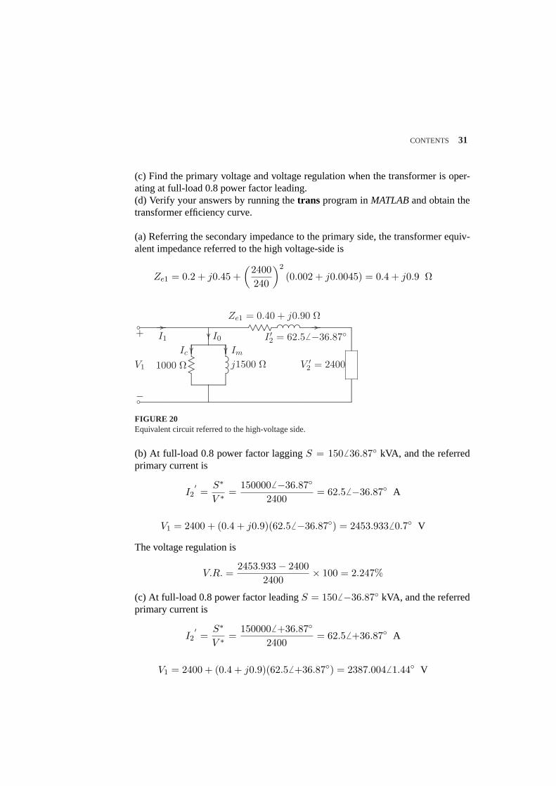
CONTENTS 31
(c) Find the primary voltage and voltage regulation when the transformer is oper-ating at full-load 0.8 power factor leading.(d) Verify your answers by running thetrans program inMATLABand obtain thetransformer efficiency curve.
(a) Referring the secondary impedance to the primary side, the transformer equiv-alent impedance referred to the high voltage-side is
Ze1 = 0.2 + j0.45 +(
2400240
)2
(0.002 + j0.0045) = 0.4 + j0.9 Ω
.................................................................................................................................................................................................................................................................................................................................................................................................................................................................................................................................................................................................................................................................................................................................................................................................................................................................................................................................................................................................................................................................................................................................................................................................................................................................................................................................
..............................................................................
..............................................................................
...........................................................................
........................................................................
.......................................................................
................. ......................... ...........
.............. ......................... ...........
.............. .........................................................................................................................................................................................................
Ze1 = 0.40 + j0.90 Ω
V1 1000 Ω j1500 Ω V ′2 = 2400
I ′2 = 62.5 6 −36.87I1 I0
Ic Im
........................................ ................ ........................................ ................
........................
........
........
........
................................
........
........
................................................................
+
−
b
bFIGURE 20Equivalent circuit referred to the high-voltage side.
(b) At full-load 0.8 power factor laggingS = 1506 36.87 kVA, and the referredprimary current is
I2′=
S∗
V ∗ =1500006 −36.87
2400= 62.56 −36.87 A
V1 = 2400 + (0.4 + j0.9)(62.5 6 −36.87) = 2453.9336 0.7 V
The voltage regulation is
V.R. =2453.933− 2400
2400× 100 = 2.247%
(c) At full-load 0.8 power factor leadingS = 1506 −36.87 kVA, and the referredprimary current is
I2′=
S∗
V ∗ =1500006 +36.87
2400= 62.56 +36.87 A
V1 = 2400 + (0.4 + j0.9)(62.56 +36.87) = 2387.0046 1.44 V
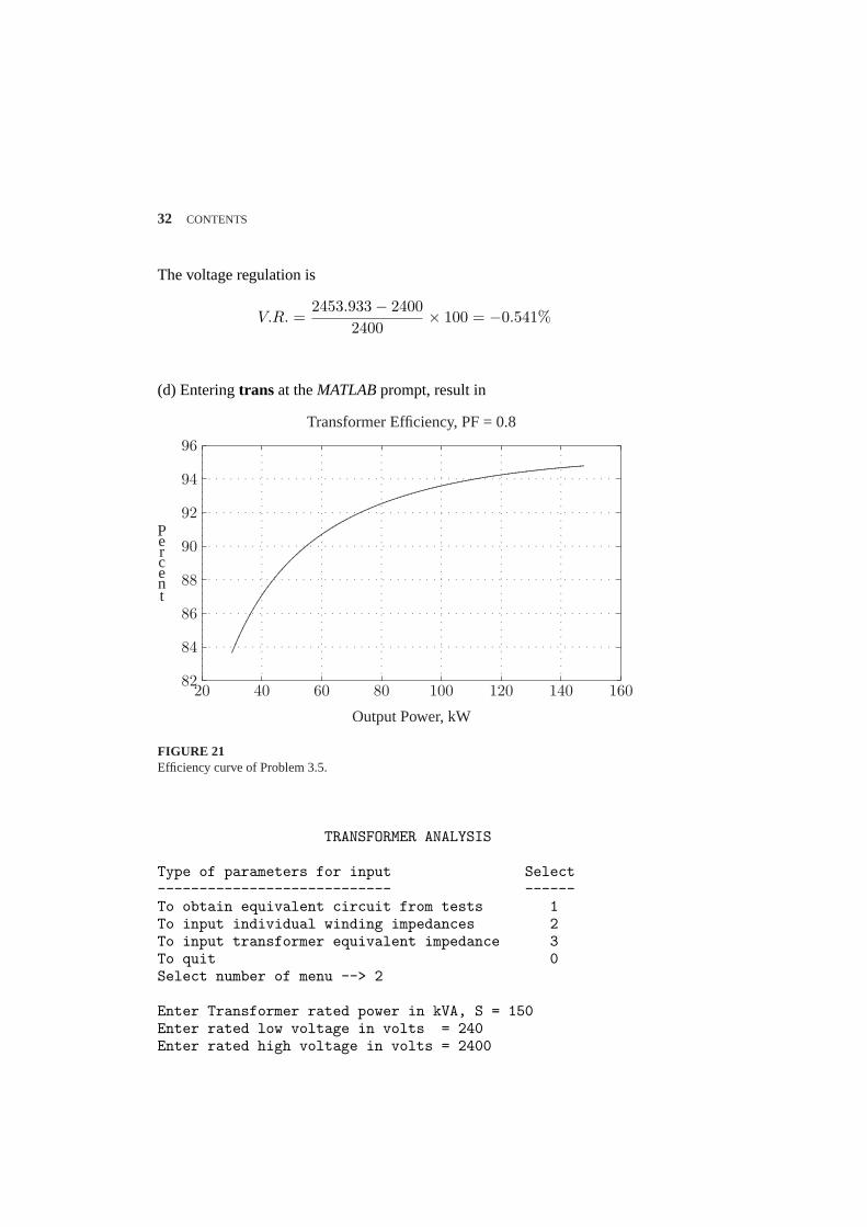
32 CONTENTS
The voltage regulation is
V.R. =2453.933− 2400
2400× 100 = −0.541%
(d) Enteringtrans at theMATLABprompt, result in
82
84
86
88
90
92
94
96
Percent
20 40 60 80 100 120 140 160
Output Power, kW
Transformer Efficiency, PF = 0.8
............................................................................................................................................................................................................................................................................................................
...................................
.......................................
...............................................
..........................................................
............................................................................
.............................................................................................................
...............................................................................................................................
.
.
.
.
.
.
.
.
.
.
.
.
.
.
.
.
.
.
.
.
.
.
.
.
.
.
.
.
.
.
.
.
.
.
.
.
.
.
.
.
.
.
.
.
.
.
.
.
.
.
.
.
.
.
.
.
.
.
.
.
.
.
.
.
.
.
.
.
.
.
.
.
.
.
.
.
.
.
.
.
.
.
.
.
.
.
.
.
.
.
.
.
.
.
.
.
.
.
.
.
.
.
.
.
.
.
.
.
.
.
.
.
.
.
.
.
.
.
.
.
.
.
.
.
.
.
.
.
.
.
.
.
.
.
.
.
.
.
.
.
.
.
.
.
.
.
.
.
.
.
.
.
.
.
.
.
.
.
.
.
.
.
.
.
.
.
.
.
.
.
.
.
.
.
.
.
.
.
.
.
.
.
.
.
.
.
.
.
.
.
.
.
.
.
.
.
.
.
.
.
.
.
.
.
.
.
.
.
.
.
.
.
.
.
.
.
.
.
.
.
.
.
.
.
.
.
.
.
.
.
.
. . . . . . . . . . . . . . . . . . . . . . . . . . . . . . . . . . . . . . . . . . . . . . . . . . . . . . . . . .
. . . . . . . . . . . . . . . . . . . . . . . . . . . . . . . . . . . . . . . . . . . . . . . . . . . . . . . . . .
. . . . . . . . . . . . . . . . . . . . . . . . . . . . . . . . . . . . . . . . . . . . . . . . . . . . . . . . . .
. . . . . . . . . . . . . . . . . . . . . . . . . . . . . . . . . . . . . . . . . . . . . . . . . . . . . . . . . .
. . . . . . . . . . . . . . . . . . . . . . . . . . . . . . . . . . . . . . . . . . . . . . . . . . . . . . . . . .
. . . . . . . . . . . . . . . . . . . . . . . . . . . . . . . . . . . . . . . . . . . . . . . . . . . . . . . . . .
FIGURE 21Efficiency curve of Problem 3.5.
TRANSFORMER ANALYSIS
Type of parameters for input Select---------------------------- ------To obtain equivalent circuit from tests 1To input individual winding impedances 2To input transformer equivalent impedance 3To quit 0Select number of menu --> 2
Enter Transformer rated power in kVA, S = 150Enter rated low voltage in volts = 240Enter rated high voltage in volts = 2400
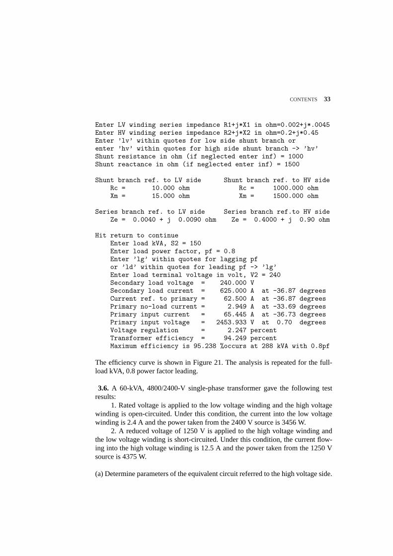
CONTENTS 33
Enter LV winding series impedance R1+j*X1 in ohm=0.002+j*.0045Enter HV winding series impedance R2+j*X2 in ohm=0.2+j*0.45Enter ’lv’ within quotes for low side shunt branch orenter ’hv’ within quotes for high side shunt branch -> ’hv’Shunt resistance in ohm (if neglected enter inf) = 1000Shunt reactance in ohm (if neglected enter inf) = 1500
Shunt branch ref. to LV side Shunt branch ref. to HV sideRc = 10.000 ohm Rc = 1000.000 ohmXm = 15.000 ohm Xm = 1500.000 ohm
Series branch ref. to LV side Series branch ref.to HV sideZe = 0.0040 + j 0.0090 ohm Ze = 0.4000 + j 0.90 ohm
Hit return to continueEnter load kVA, S2 = 150Enter load power factor, pf = 0.8Enter ’lg’ within quotes for lagging pfor ’ld’ within quotes for leading pf -> ’lg’Enter load terminal voltage in volt, V2 = 240Secondary load voltage = 240.000 VSecondary load current = 625.000 A at -36.87 degreesCurrent ref. to primary = 62.500 A at -36.87 degreesPrimary no-load current = 2.949 A at -33.69 degreesPrimary input current = 65.445 A at -36.73 degreesPrimary input voltage = 2453.933 V at 0.70 degreesVoltage regulation = 2.247 percentTransformer efficiency = 94.249 percentMaximum efficiency is 95.238 %occurs at 288 kVA with 0.8pf
The efficiency curve is shown in Figure 21. The analysis is repeated for the full-load kVA, 0.8 power factor leading.
3.6. A 60-kVA, 4800/2400-V single-phase transformer gave the following testresults:
1. Rated voltage is applied to the low voltage winding and the high voltagewinding is open-circuited. Under this condition, the current into the low voltagewinding is 2.4 A and the power taken from the 2400 V source is 3456 W.
2. A reduced voltage of 1250 V is applied to the high voltage winding andthe low voltage winding is short-circuited. Under this condition, the current flow-ing into the high voltage winding is 12.5 A and the power taken from the 1250 Vsource is 4375 W.
(a) Determine parameters of the equivalent circuit referred to the high voltage side.
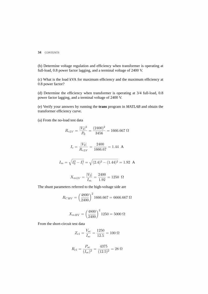
34 CONTENTS
(b) Determine voltage regulation and efficiency when transformer is operating atfull-load, 0.8 power factor lagging, and a terminal voltage of 2400 V.
(c) What is the load kVA for maximum efficiency and the maximum efficiency at0.8 power factor?
(d) Determine the efficiency when transformer is operating at 3/4 full-load, 0.8power factor lagging, and a terminal voltage of 2400 V.
(e) Verify your answers by running thetrans program inMATLABand obtain thetransformer efficiency curve.
(a) From the no-load test data
RcLV =|V2|2P0
=(2400)2
3456= 1666.667 Ω
Ic =|V2|
RcLV=
24001666.67
= 1.44 A
Im =√
I20 − I2
c =√
(2.4)2 − (1.44)2 = 1.92 A
XmLV =|V2|Im
=24001.92
= 1250 Ω
The shunt parameters referred to the high-voltage side are
RCHV =(
48002400
)2
1666.667 = 6666.667 Ω
XmHV =(
48002400
)2
1250 = 5000 Ω
From the short-circuit test data
Ze1 =Vsc
Isc=
125012.5
= 100 Ω
Re1 =Psc
(Isc)2=
4375(12.5)2
= 28 Ω
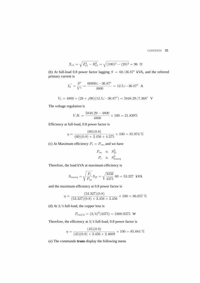
CONTENTS 35
Xe1 =√
Z2e1 −R2
e1 =√
(100)2 − (28)2 = 96 Ω
(b) At full-load 0.8 power factor laggingS = 606 36.87 kVA, and the referredprimary current is
I2′=
S∗
V ∗ =600006 −36.87
4800= 12.56 −36.87 A
V1 = 4800 + (28 + j96)(12.56 −36.87) = 5848.29 6 7.368 V
The voltage regulation is
V.R. =5848.29− 4800
4800× 100 = 21.839%
Efficiency at full-load, 0.8 power factor is
η =(60)(0.8)
(60)(0.8) + 3.456 + 4.375× 100 = 85.974 %
(c) At Maximum efficiencyPc = Pcu, and we have
Pcu ∝ S2fl
Pc ∝ S2maxη
Therefore, the load kVA at maximum efficiency is
Smaxη =
√Pc
PcuSfl =
√34564375
60 = 53.327 kVA
and the maximum efficiency at 0.8 power factor is
η =(53.327)(0.8)
(53.327)(0.8) + 3.456 + 3.456× 100 = 86.057 %
(d) At 3/4 full-load, the copper loss is
Pcu3/4 = (3/4)2(4375) = 2460.9375 W
Therefore, the efficiency at3/4 full-load, 0.8 power factor is
η =(45)(0.8)
(45)(0.8) + 3.456 + 2.4609× 100 = 85.884 %
(e) The commandstrans display the following menu
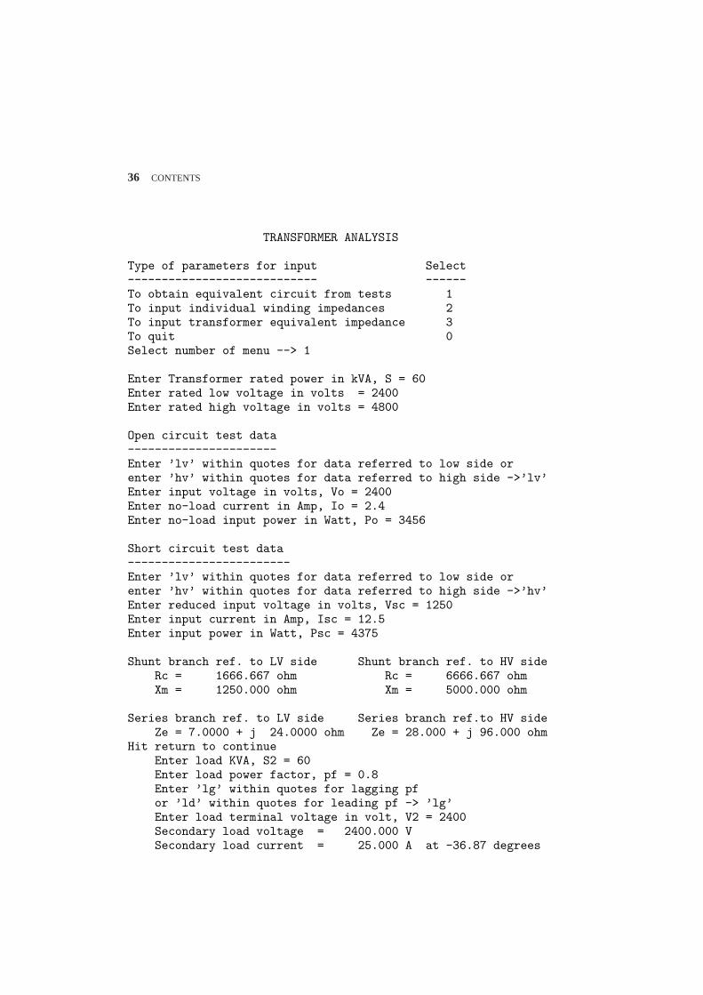
36 CONTENTS
TRANSFORMER ANALYSIS
Type of parameters for input Select---------------------------- ------To obtain equivalent circuit from tests 1To input individual winding impedances 2To input transformer equivalent impedance 3To quit 0Select number of menu --> 1
Enter Transformer rated power in kVA, S = 60Enter rated low voltage in volts = 2400Enter rated high voltage in volts = 4800
Open circuit test data----------------------Enter ’lv’ within quotes for data referred to low side orenter ’hv’ within quotes for data referred to high side ->’lv’Enter input voltage in volts, Vo = 2400Enter no-load current in Amp, Io = 2.4Enter no-load input power in Watt, Po = 3456
Short circuit test data------------------------Enter ’lv’ within quotes for data referred to low side orenter ’hv’ within quotes for data referred to high side ->’hv’Enter reduced input voltage in volts, Vsc = 1250Enter input current in Amp, Isc = 12.5Enter input power in Watt, Psc = 4375
Shunt branch ref. to LV side Shunt branch ref. to HV sideRc = 1666.667 ohm Rc = 6666.667 ohmXm = 1250.000 ohm Xm = 5000.000 ohm
Series branch ref. to LV side Series branch ref.to HV sideZe = 7.0000 + j 24.0000 ohm Ze = 28.000 + j 96.000 ohm
Hit return to continueEnter load KVA, S2 = 60Enter load power factor, pf = 0.8Enter ’lg’ within quotes for lagging pfor ’ld’ within quotes for leading pf -> ’lg’Enter load terminal voltage in volt, V2 = 2400Secondary load voltage = 2400.000 VSecondary load current = 25.000 A at -36.87 degrees
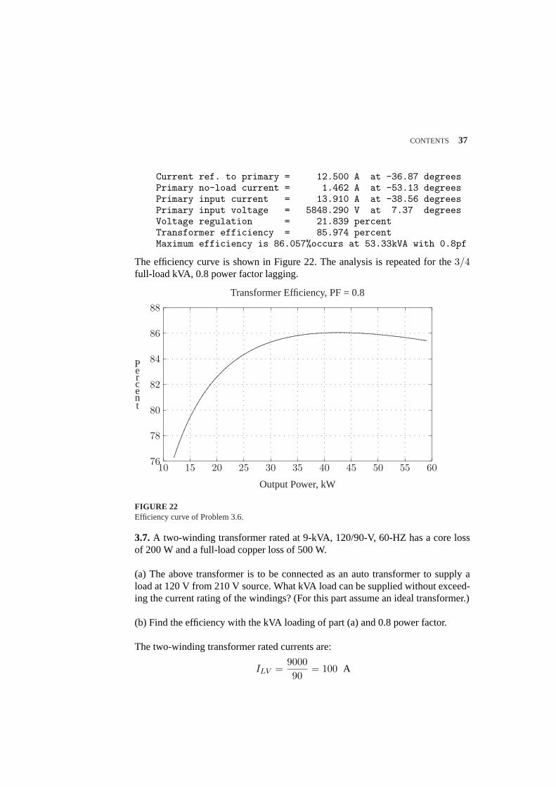
CONTENTS 37
Current ref. to primary = 12.500 A at -36.87 degreesPrimary no-load current = 1.462 A at -53.13 degreesPrimary input current = 13.910 A at -38.56 degreesPrimary input voltage = 5848.290 V at 7.37 degreesVoltage regulation = 21.839 percentTransformer efficiency = 85.974 percentMaximum efficiency is 86.057%occurs at 53.33kVA with 0.8pf
The efficiency curve is shown in Figure 22. The analysis is repeated for the3/4full-load kVA, 0.8 power factor lagging.
76
78
80
82
84
86
88
Percent
10 15 20 25 30 35 40 45 50 55 60
Output Power, kW
Transformer Efficiency, PF = 0.8
...............................................................................................................................................................................................................................................................................................................................................................................
..................................
...............................................
...........................................................................
....................................................................................................................................................................................................................................................................................................................................................................
.
.
.
.
.
.
.
.
.
.
.
.
.
.
.
.
.
.
.
.
.
.
.
.
.
.
.
.
.
.
.
.
.
.
.
.
.
.
.
.
.
.
.
.
.
.
.
.
.
.
.
.
.
.
.
.
.
.
.
.
.
.
.
.
.
.
.
.
.
.
.
.
.
.
.
.
.
.
.
.
.
.
.
.
.
.
.
.
.
.
.
.
.
.
.
.
.
.
.
.
.
.
.
.
.
.
.
.
.
.
.
.
.
.
.
.
.
.
.
.
.
.
.
.
.
.
.
.
.
.
.
.
.
.
.
.
.
.
.
.
.
.
.
.
.
.
.
.
.
.
.
.
.
.
.
.
.
.
.
.
.
.
.
.
.
.
.
.
.
.
.
.
.
.
.
.
.
.
.
.
.
.
.
.
.
.
.
.
.
.
.
.
.
.
.
.
.
.
.
.
.
.
.
.
.
.
.
.
.
.
.
.
.
.
.
.
.
.
.
.
.
.
.
.
.
.
.
.
.
.
.
.
.
.
.
.
.
.
.
.
.
.
.
.
.
.
.
.
.
.
.
.
.
.
.
.
.
.
.
.
.
.
.
.
.
.
.
.
.
.
.
.
.
.
.
.
.
.
.
.
.
.
.
.
.
.
.
.
.
.
.
.
.
.
.
.
.
. . . . . . . . . . . . . . . . . . . . . . . . . . . . . . . . . . . . . . . . . . . . . . . . . . . . . . . . . .
. . . . . . . . . . . . . . . . . . . . . . . . . . . . . . . . . . . . . . . . . . . . . . . . . . . . . . . . . .
. . . . . . . . . . . . . . . . . . . . . . . . . . . . . . . . . . . . . . . . . . . . . . . . . . . . . . . . . .
. . . . . . . . . . . . . . . . . . . . . . . . . . . . . . . . . . . . . . . . . . . . . . . . . . . . . . . . . .
. . . . . . . . . . . . . . . . . . . . . . . . . . . . . . . . . . . . . . . . . . . . . . . . . . . . . . . . . .
FIGURE 22Efficiency curve of Problem 3.6.
3.7.A two-winding transformer rated at 9-kVA, 120/90-V, 60-HZ has a core lossof 200 W and a full-load copper loss of 500 W.
(a) The above transformer is to be connected as an auto transformer to supply aload at 120 V from 210 V source. What kVA load can be supplied without exceed-ing the current rating of the windings? (For this part assume an ideal transformer.)
(b) Find the efficiency with the kVA loading of part (a) and 0.8 power factor.
The two-winding transformer rated currents are:
ILV =900090
= 100 A
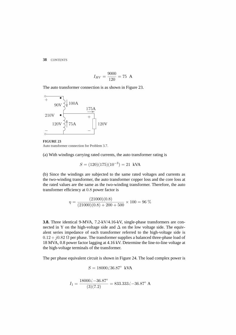
38 CONTENTS
IHV =9000120
= 75 A
The auto transformer connection is as shown in Figure 23.
...................................................................................................................................
.................................................................................................................................................................................................................................................................................................................................................
............................................
.....................................................................................................................................................................................................................................
.........................................................................................................
............................................................................................................................................
........
........
......
....................................................
........
........
........
........
........
........
........
........
....................
................
............................................................ ................
210V
90V
120V
100A
75A
175A
+
−
+
−120V
•
•
FIGURE 23Auto transformer connection for Problem 3.7.
(a) With windings carrying rated currents, the auto transformer rating is
S = (120)(175)(10−3) = 21 kVA
(b) Since the windings are subjected to the same rated voltages and currents asthe two-winding transformer, the auto transformer copper loss and the core loss atthe rated values are the same as the two-winding transformer. Therefore, the autotransformer efficiency at0.8 power factor is
η =(21000)(0.8)
(21000)(0.8) + 200 + 500× 100 = 96 %
3.8. Three identical 9-MVA, 7.2-kV/4.16-kV, single-phase transformers are con-nected in Y on the high-voltage side and∆ on the low voltage side. The equiv-alent series impedance of each transformer referred to the high-voltage side is0.12+ j0.82 Ω per phase. The transformer supplies a balanced three-phase load of18 MVA, 0.8 power factor lagging at 4.16 kV. Determine the line-to-line voltage atthe high-voltage terminals of the transformer.
The per phase equivalent circuit is shown in Figure 24. The load complex power is
S = 180006 36.87 kVA
I1 =180006 −36.87
(3)(7.2)= 833.3336 −36.87 A
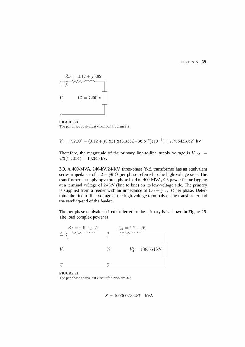
CONTENTS 39
......................................................................................................................................
.......................................................................
................. ......................... ...........
.............. ......................... ...........
..............
....................................................................................................................................................................................................................................................................................................................................
............................................................................................................................
Ze1 = 0.12 + j0.82
V1 V ′2 = 7200 V
I1
........................................ ................
+
−
b
bFIGURE 24The per phase equivalent circuit of Problem 3.8.
V1 = 7.26 0 + (0.12 + j0.82)(833.3336 −36.87)(10−3)= 7.7054 6 3.62 kV
Therefore, the magnitude of the primary line-to-line supply voltage isV1LL =√3(7.7054) = 13.346 kV.
3.9.A 400-MVA, 240-kV/24-KV, three-phase Y-∆ transformer has an equivalentseries impedance of1.2 + j6 Ω per phase referred to the high-voltage side. Thetransformer is supplying a three-phase load of 400-MVA, 0.8 power factor laggingat a terminal voltage of 24 kV (line to line) on its low-voltage side. The primaryis supplied from a feeder with an impedance of0.6 + j1.2 Ω per phase. Deter-mine the line-to-line voltage at the high-voltage terminals of the transformer andthe sending-end of the feeder.
The per phase equivalent circuit referred to the primary is is shown in Figure 25.The load complex power is
......................................................................................................................................
.......................................................................
................. ......................... ...........
.............. ......................... ...........
.............. ............................................................................. ......................................................................
.....................................................................................................................................................................................................................................................................................
........................................................................................................................................................................................................................................................................................................................................................................................................................
+
−
V1
........................................................................
.......................................................................
................. ......................... ...........
.............. ......................... ...........
.............. .........................................................................................................................................................................................................
Zf = 0.6 + j1.2 Ze1 = 1.2 + j6
Vs V ′2 = 138.564 kV
I1
........................................ ................
+
−
b
bFIGURE 25The per phase equivalent circuit for Problem 3.9.
S = 4000006 36.87 kVA
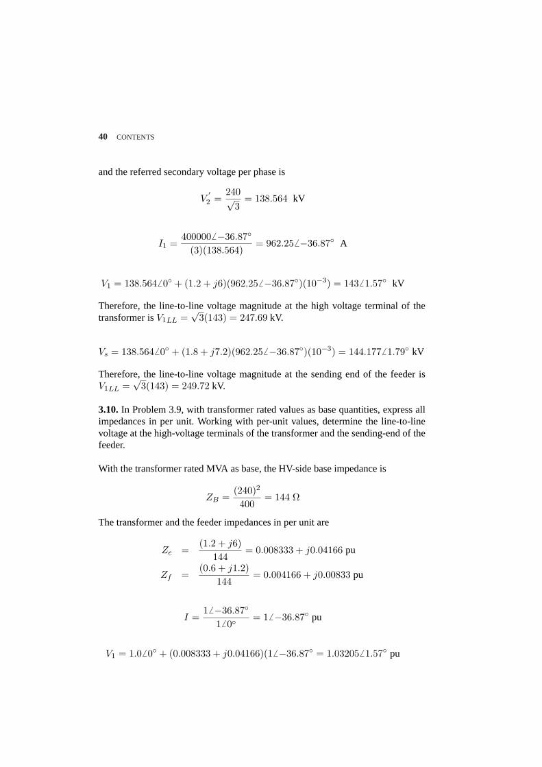
40 CONTENTS
and the referred secondary voltage per phase is
V′2 =
240√3
= 138.564 kV
I1 =4000006 −36.87
(3)(138.564)= 962.256 −36.87 A
V1 = 138.5646 0 + (1.2 + j6)(962.256 −36.87)(10−3) = 1436 1.57 kV
Therefore, the line-to-line voltage magnitude at the high voltage terminal of thetransformer isV1LL =
√3(143) = 247.69 kV.
Vs = 138.5646 0 + (1.8 + j7.2)(962.256 −36.87)(10−3) = 144.1776 1.79 kV
Therefore, the line-to-line voltage magnitude at the sending end of the feeder isV1LL =
√3(143) = 249.72 kV.
3.10.In Problem 3.9, with transformer rated values as base quantities, express allimpedances in per unit. Working with per-unit values, determine the line-to-linevoltage at the high-voltage terminals of the transformer and the sending-end of thefeeder.
With the transformer rated MVA as base, the HV-side base impedance is
ZB =(240)2
400= 144 Ω
The transformer and the feeder impedances in per unit are
Ze =(1.2 + j6)
144= 0.008333 + j0.04166 pu
Zf =(0.6 + j1.2)
144= 0.004166 + j0.00833 pu
I =1 6 −36.87
16 0= 16 −36.87 pu
V1 = 1.06 0 + (0.008333 + j0.04166)(16 −36.87 = 1.032056 1.57 pu
CONTENTS 41
Therefore, the line-to-line voltage magnitude at the high-voltage terminal of thetransformer is(1.03205)(240) = 247.69 kV
Vs = 1.06 0 + (0.0125 + j0.05)(16 −36.87 = 1.04056 1.79 pu
Therefore, the line-to-line voltage magnitude at the high voltage terminal of thetransformer is(1.0405)(240) = 249.72 kV
3.11.A three-phase, Y-connected, 75-MVA, 27-kV synchronous generator has asynchronous reactance of9.0 Ω per phase. Using rated MVA and voltage as basevalues, determine the per unit reactance. Then refer this per unit value to a 100-MVA, 30-kV base.
The base impedance is
ZB =(KVB)2
MV AB=
(27)2
75= 9.72 Ω
Xpu =9
9.72= 0.926 pu
The generator reactance on a 100-MVA, 30-kV base is
Xpunew = 0.926(
10075
) (2730
)2
= 1.0 pu
3.12.A 40-MVA, 20-kV/400-kV, single-phase transformer has the following seriesimpedances:
Z1 = 0.9 + j1.8 Ω and Z2 = 128 + j288 ΩUsing the transformer rating as base, determine the per unit impedance of the trans-former from the ohmic value referred to the low-voltage side. Compute the per unitimpedance using the ohmic value referred to the high-voltage side.
The transformer equivalent impedance referred to the low-voltage side is
Ze1 = 0.9 + j1.8 +(
20400
)2
(128 + j288) = 1.22 + j2.52 Ω
The low-voltage base impedance is
ZB1 =(20)2
40= 10 Ω
Zpu1 =1.22 + j2.52
10= 0.122 + j0.252 pu
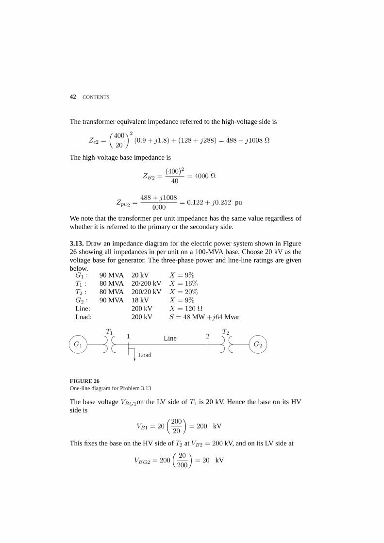
42 CONTENTS
The transformer equivalent impedance referred to the high-voltage side is
Ze2 =(
40020
)2
(0.9 + j1.8) + (128 + j288) = 488 + j1008 Ω
The high-voltage base impedance is
ZB2 =(400)2
40= 4000 Ω
Zpu2 =488 + j1008
4000= 0.122 + j0.252 pu
We note that the transformer per unit impedance has the same value regardless ofwhether it is referred to the primary or the secondary side.
3.13.Draw an impedance diagram for the electric power system shown in Figure26 showing all impedances in per unit on a 100-MVA base. Choose 20 kV as thevoltage base for generator. The three-phase power and line-line ratings are givenbelow.
G1 : 90 MVA 20 kV X = 9%T1 : 80 MVA 20/200 kV X = 16%T2 : 80 MVA 200/20 kV X = 20%G2 : 90 MVA 18 kV X = 9%Line: 200 kV X = 120 ΩLoad: 200 kV S = 48 MW +j64 Mvar
.............................................
.......
.............................................
.......
........................................................................................................
.............................................
.......
.............................................
.......
........................................................................................................
?½¼
¾»
½¼
¾»G1
T1 T2
G2
1 2Line
Load
FIGURE 26One-line diagram for Problem 3.13
The base voltageVBG1on the LV side ofT1 is 20 kV. Hence the base on its HVside is
VB1 = 20(
20020
)= 200 kV
This fixes the base on the HV side ofT2 atVB2 = 200 kV, and on its LV side at
VBG2 = 200(
20200
)= 20 kV
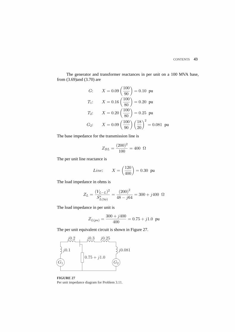
CONTENTS 43
The generator and transformer reactances in per unit on a 100 MVA base,from (3.69)and (3.70) are
G: X = 0.09(
10090
)= 0.10 pu
T1: X = 0.16(
10080
)= 0.20 pu
T2: X = 0.20(
10080
)= 0.25 pu
G2: X = 0.09(
10090
) (1820
)2
= 0.081 pu
The base impedance for the transmission line is
ZBL =(200)2
100= 400 Ω
The per unit line reactance is
Line: X =(
120400
)= 0.30 pu
The load impedance in ohms is
ZL =(VL−L)2
S∗L(3φ)
=(200)2
48− j64= 300 + j400 Ω
The load impedance in per unit is
ZL(pu) =300 + j400
400= 0.75 + j1.0 pu
The per unit equivalent circuit is shown in Figure 27.
µ´¶³G1
j0.1.......................
.........................
.........................
..
µ´¶³G2
j0.081.......................
.........................
.........................
..
....................................
.......................................
j0.2....................................
.......................................
j0.3....................................
.......................................
j0.25
0.75 + j1.0
FIGURE 27Per unit impedance diagram for Problem 3.11.
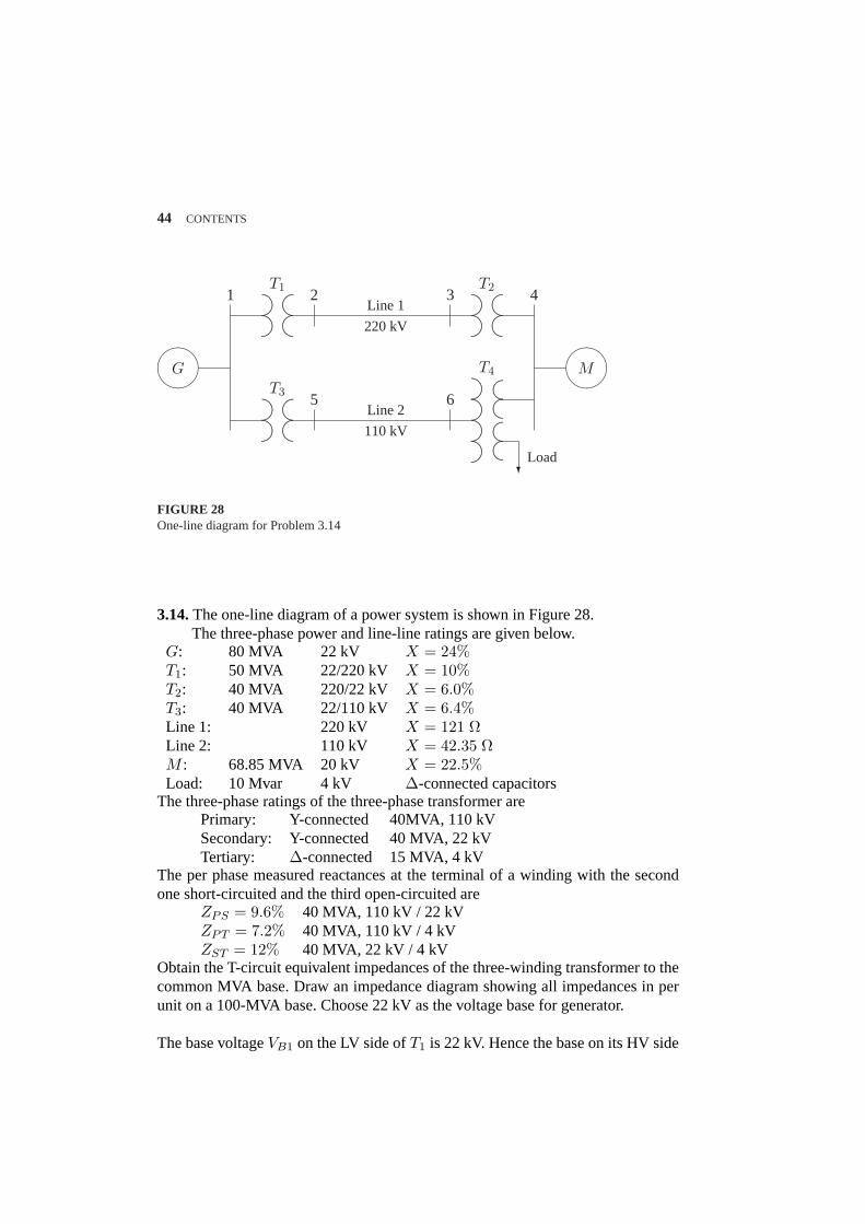
44 CONTENTS
.............................................
............
.............................................
............
..................................................................................................................
.............................................
............
.............................................
............
..................................................................................................................
.............................................
............
.............................................
............
..................................................................................................................
.............................................
............
.............................................
............
.............................................
............
.............................................
............
................................................................................................................................................................................................................
?
½¼
¾»
½¼
¾»G
T1 T2
T3
T4 M
1 2 3 4
5 6
Line 1
Line 2
Load
220 kV
110 kV
FIGURE 28One-line diagram for Problem 3.14
3.14.The one-line diagram of a power system is shown in Figure 28.The three-phase power and line-line ratings are given below.
G: 80 MVA 22 kV X = 24%T1: 50 MVA 22/220 kV X = 10%T2: 40 MVA 220/22 kV X = 6.0%T3: 40 MVA 22/110 kV X = 6.4%Line 1: 220 kV X = 121 ΩLine 2: 110 kV X = 42.35 ΩM : 68.85 MVA 20 kV X = 22.5%Load: 10 Mvar 4 kV ∆-connected capacitors
The three-phase ratings of the three-phase transformer arePrimary: Y-connected 40MVA, 110 kVSecondary: Y-connected 40 MVA, 22 kVTertiary: ∆-connected 15 MVA, 4 kV
The per phase measured reactances at the terminal of a winding with the secondone short-circuited and the third open-circuited are
ZPS = 9.6% 40 MVA, 110 kV / 22 kVZPT = 7.2% 40 MVA, 110 kV / 4 kVZST = 12% 40 MVA, 22 kV / 4 kV
Obtain the T-circuit equivalent impedances of the three-winding transformer to thecommon MVA base. Draw an impedance diagram showing all impedances in perunit on a 100-MVA base. Choose 22 kV as the voltage base for generator.
The base voltageVB1 on the LV side ofT1 is 22 kV. Hence the base on its HV side
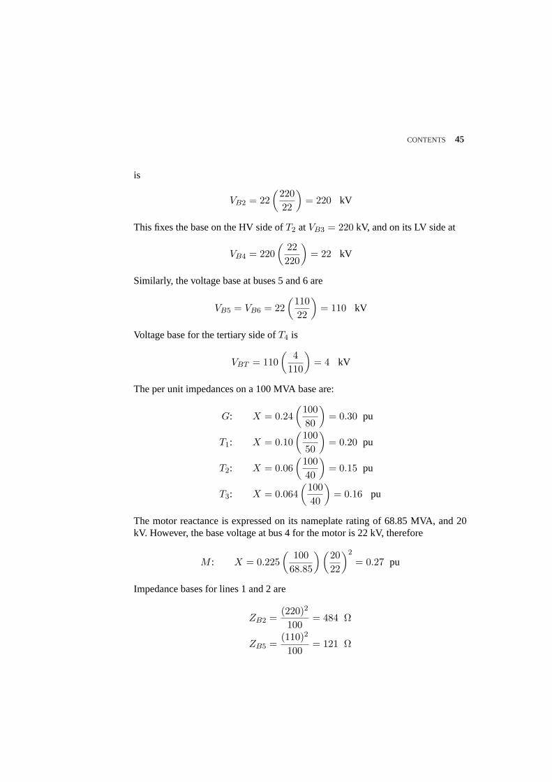
CONTENTS 45
is
VB2 = 22(
22022
)= 220 kV
This fixes the base on the HV side ofT2 atVB3 = 220 kV, and on its LV side at
VB4 = 220(
22220
)= 22 kV
Similarly, the voltage base at buses 5 and 6 are
VB5 = VB6 = 22(
11022
)= 110 kV
Voltage base for the tertiary side ofT4 is
VBT = 110(
4110
)= 4 kV
The per unit impedances on a 100 MVA base are:
G: X = 0.24(
10080
)= 0.30 pu
T1: X = 0.10(
10050
)= 0.20 pu
T2: X = 0.06(
10040
)= 0.15 pu
T3: X = 0.064(
10040
)= 0.16 pu
The motor reactance is expressed on its nameplate rating of 68.85 MVA, and 20kV. However, the base voltage at bus 4 for the motor is 22 kV, therefore
M : X = 0.225(
10068.85
) (2022
)2
= 0.27 pu
Impedance bases for lines 1 and 2 are
ZB2 =(220)2
100= 484 Ω
ZB5 =(110)2
100= 121 Ω
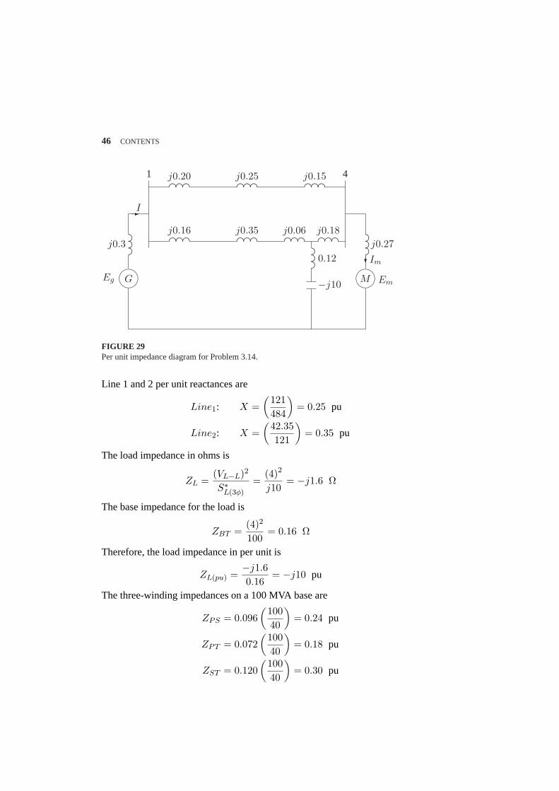
46 CONTENTS
............................. ..........
................... ............................. ..........
................... ............................. ..........
................... ............................. ..........
................... .............................
............................. ..........
................... ............................. ..........
................... ............................. ..........
................... ............................. ..........
................... ............................. ..........
................... ............................. ..........
................................................
.............................
.............................
µ´¶³ .............
..........................................................................
.............................
.............................
.............................
?Im
µ´¶³
G M
1 4j0.20 j0.25 j0.15
j0.16 j0.35 j0.06 j0.18j0.3 j0.27
0.12
−j10Eg Em
-I
FIGURE 29Per unit impedance diagram for Problem 3.14.
Line 1 and 2 per unit reactances are
Line1: X =(
121484
)= 0.25 pu
Line2: X =(
42.35121
)= 0.35 pu
The load impedance in ohms is
ZL =(VL−L)2
S∗L(3φ)
=(4)2
j10= −j1.6 Ω
The base impedance for the load is
ZBT =(4)2
100= 0.16 Ω
Therefore, the load impedance in per unit is
ZL(pu) =−j1.60.16
= −j10 pu
The three-winding impedances on a 100 MVA base are
ZPS = 0.096(
10040
)= 0.24 pu
ZPT = 0.072(
10040
)= 0.18 pu
ZST = 0.120(
10040
)= 0.30 pu
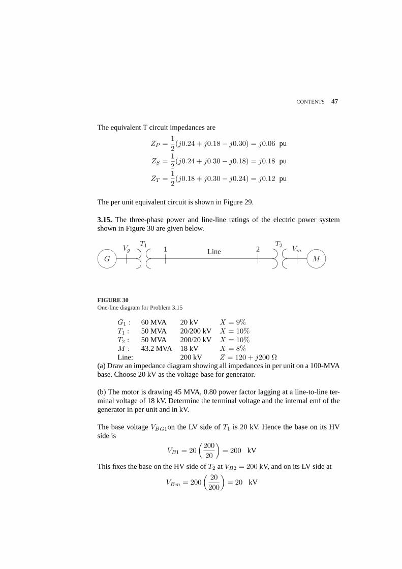
CONTENTS 47
The equivalent T circuit impedances are
ZP =12(j0.24 + j0.18− j0.30) = j0.06 pu
ZS =12(j0.24 + j0.30− j0.18) = j0.18 pu
ZT =12(j0.18 + j0.30− j0.24) = j0.12 pu
The per unit equivalent circuit is shown in Figure 29.
3.15. The three-phase power and line-line ratings of the electric power systemshown in Figure 30 are given below.
.............................................
............
.............................................
............
..................................................................................................................
.........................................................
.............................................
............
..................................................................................................................½¼
¾»
½¼
¾»G
Vg VmT1 T2
M
1 2Line
FIGURE 30One-line diagram for Problem 3.15
G1 : 60 MVA 20 kV X = 9%T1 : 50 MVA 20/200 kV X = 10%T2 : 50 MVA 200/20 kV X = 10%M : 43.2 MVA 18 kV X = 8%Line: 200 kV Z = 120 + j200 Ω
(a) Draw an impedance diagram showing all impedances in per unit on a 100-MVAbase. Choose 20 kV as the voltage base for generator.
(b) The motor is drawing 45 MVA, 0.80 power factor lagging at a line-to-line ter-minal voltage of 18 kV. Determine the terminal voltage and the internal emf of thegenerator in per unit and in kV.
The base voltageVBG1on the LV side ofT1 is 20 kV. Hence the base on its HVside is
VB1 = 20(
20020
)= 200 kV
This fixes the base on the HV side ofT2 atVB2 = 200 kV, and on its LV side at
VBm = 200(
20200
)= 20 kV
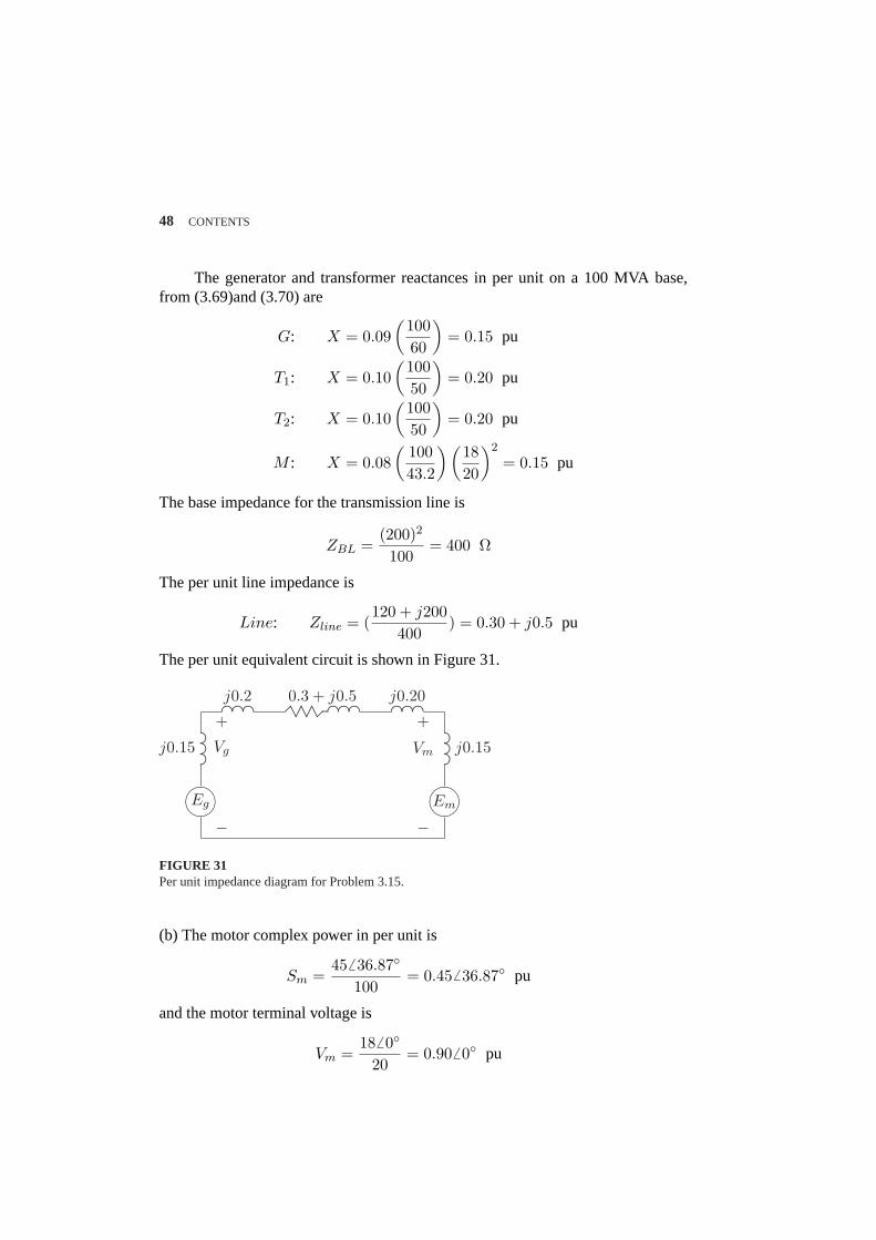
48 CONTENTS
The generator and transformer reactances in per unit on a 100 MVA base,from (3.69)and (3.70) are
G: X = 0.09(
10060
)= 0.15 pu
T1: X = 0.10(
10050
)= 0.20 pu
T2: X = 0.10(
10050
)= 0.20 pu
M : X = 0.08(
10043.2
) (1820
)2
= 0.15 pu
The base impedance for the transmission line is
ZBL =(200)2
100= 400 Ω
The per unit line impedance is
Line: Zline = (120 + j200
400) = 0.30 + j0.5 pu
The per unit equivalent circuit is shown in Figure 31.
µ´¶³Eg
j0.15 Vg
+
−
Vm
+
−
.......................................................................................
µ´¶³Em
j0.15.......................................................................................
.......................................
................................................
j0.2...........................................
..........................................
............................................
...................................................
................................................
0.3 + j0.5.......................................
................................................
j0.20
FIGURE 31Per unit impedance diagram for Problem 3.15.
(b) The motor complex power in per unit is
Sm =456 36.87
100= 0.456 36.87 pu
and the motor terminal voltage is
Vm =186 0
20= 0.906 0 pu
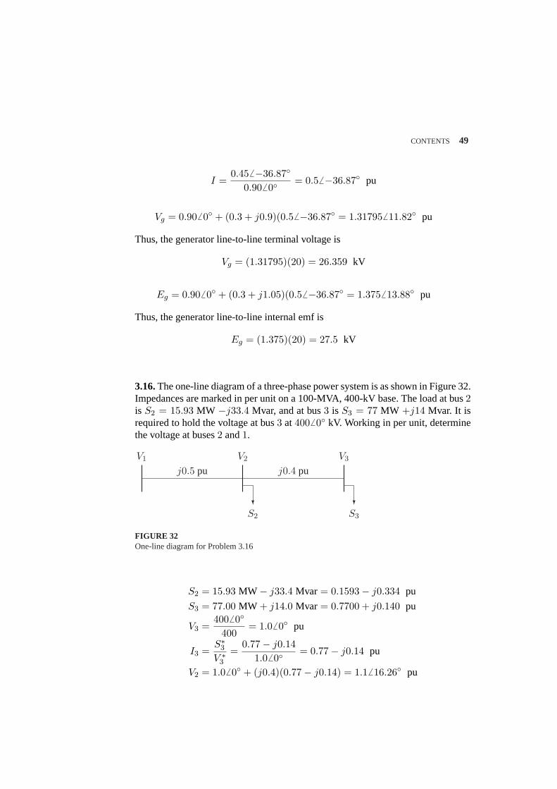
CONTENTS 49
I =0.456 −36.87
0.906 0= 0.56 −36.87 pu
Vg = 0.906 0 + (0.3 + j0.9)(0.56 −36.87 = 1.317956 11.82 pu
Thus, the generator line-to-line terminal voltage is
Vg = (1.31795)(20) = 26.359 kV
Eg = 0.906 0 + (0.3 + j1.05)(0.5 6 −36.87 = 1.3756 13.88 pu
Thus, the generator line-to-line internal emf is
Eg = (1.375)(20) = 27.5 kV
3.16.The one-line diagram of a three-phase power system is as shown in Figure 32.Impedances are marked in per unit on a 100-MVA, 400-kV base. The load at bus2is S2 = 15.93 MW −j33.4 Mvar, and at bus3 is S3 = 77 MW +j14 Mvar. It isrequired to hold the voltage at bus3 at4006 0 kV. Working in per unit, determinethe voltage at buses2 and1.
? ?
V1 V2 V3
S2 S3
j0.5 pu j0.4 pu
FIGURE 32One-line diagram for Problem 3.16
S2 = 15.93 MW − j33.4 Mvar = 0.1593− j0.334 pu
S3 = 77.00 MW + j14.0 Mvar = 0.7700 + j0.140 pu
V3 =4006 0
400= 1.0 6 0 pu
I3 =S∗3V ∗
3
=0.77− j0.14
1.06 0= 0.77− j0.14 pu
V2 = 1.0 6 0 + (j0.4)(0.77− j0.14) = 1.16 16.26 pu
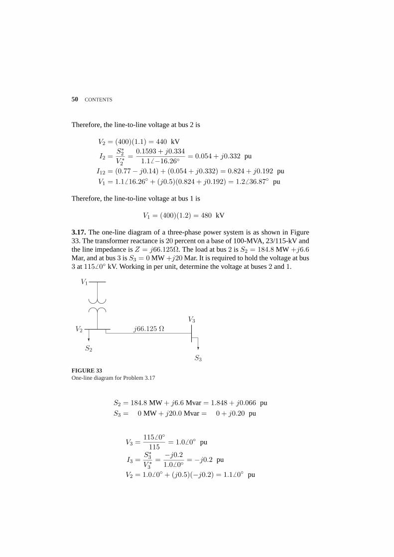
50 CONTENTS
Therefore, the line-to-line voltage at bus 2 is
V2 = (400)(1.1) = 440 kV
I2 =S∗2V ∗
2
=0.1593 + j0.334
1.16 −16.26= 0.054 + j0.332 pu
I12 = (0.77− j0.14) + (0.054 + j0.332) = 0.824 + j0.192 pu
V1 = 1.16 16.26 + (j0.5)(0.824 + j0.192) = 1.26 36.87 pu
Therefore, the line-to-line voltage at bus 1 is
V1 = (400)(1.2) = 480 kV
3.17.The one-line diagram of a three-phase power system is as shown in Figure33. The transformer reactance is20 percent on a base of 100-MVA, 23/115-kV andthe line impedance isZ = j66.125Ω. The load at bus2 is S2 = 184.8 MW +j6.6Mar, and at bus3 is S3 = 0 MW +j20 Mar. It is required to hold the voltage at bus3 at1156 0 kV. Working in per unit, determine the voltage at buses2 and1.
..............................................................................................
..........
............................................................
............................................
??
V1
V2
V3
S2
S3
j66.125 Ω
FIGURE 33One-line diagram for Problem 3.17
S2 = 184.8 MW + j6.6 Mvar = 1.848 + j0.066 pu
S3 = 0 MW + j20.0 Mvar = 0 + j0.20 pu
V3 =1156 0
115= 1.06 0 pu
I3 =S∗3V ∗
3
=−j0.21.0 6 0
= −j0.2 pu
V2 = 1.06 0 + (j0.5)(−j0.2) = 1.1 6 0 pu
CONTENTS 51
Therefore, the line-to-line voltage at bus 2 is
V2 = (115)(1.1) = 126.5 kV
I2 =S∗2V ∗
2
=1.848− j0.066
1.16 0= 1.68− j0.06 pu
I12 = (1.68− j0.06) + (−j0.2) = 1.68− j0.26 pu
V1 = 1.1 6 0 + (j0.2)(1.68− j0.26) = 1.26 16.26 pu
Therefore, the line-to-line voltage at bus 1 is
V1 = (23)(1.2) = 27.6 kV
CHAPTER 4 PROBLEMS
4.1. A solid cylindrical aluminum conductor 25 km long has an area of 336,400circular mils. Obtain the conductor resistance at (a)20C and (b)50C. The resis-tivity of aluminum at20C is2.8× 10−8 Ω-m.
(a)
d =√
336400 = 580 mil = (580)(10−3)(2.54) = 1.4732 cm
A =πd2
4= 1.704564 cm2
R1 = ρ`
A= 2.8× 10⁻⁸ 25× 103
1.704564× 10−4= 4.106 Ω
(b)
R2 = R1
(228 + 50228 + 20
)= 4.106
(278248
)= 4.6 Ω
4.2. A transmission-line cable consists of 12 identical strands of aluminum, each3 mm in diameter. The resistivity of aluminum strand at20C is 2.8× 10⁻⁸ Ω-m.Find the50C AC resistance per Km of the cable. Assume a skin-effect correctionfactor of 1.02 at 60 Hz.
52
CONTENTS 53
A = 12πd2
4= 12
(π)(32)4
= 84.823 mm2
R20 = ρ`
A=
2.8× 10−8 × 103
84.823× 10−6= 0.33 Ω
R50 = R20
(228 + 50228 + 20
)= 0.33
(278248
)= 0.37 Ω
RAC = (1.02)(0.37) = 0.3774 Ω
4.3. A three-phase transmission line is designed to deliver 190.5-MVA at 220-kV over a distance of 63 Km. The total transmission line loss is not to exceed2.5 percent of the rated line MVA. If the resistivity of the conductor material is2.84 × 10−8 Ω-m, determine the required conductor diameter and the conductorsize in circular mils.
The total transmission line loss is
PL =2.5100
(190.5) = 4.7625 MW
|I| = S√3VL
=(190.5)103
√3(220)
= 500 A
FromPL = 3R|I|2, the line resistance per phase is
R =4.7625× 10⁶
3(500)2= 6.35 Ω
The conductor cross sectional area is
A =(2.84× 10⁻⁸)(63× 103)
6.35= 2.81764× 10⁻⁴ m2
Therefore
d = 1.894 cm = 0.7456 in = 556000 cmil
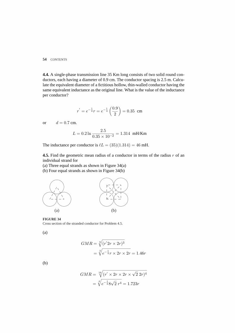
54 CONTENTS
4.4.A single-phase transmission line 35 Km long consists of two solid round con-ductors, each having a diameter of 0.9 cm. The conductor spacing is 2.5 m. Calcu-late the equivalent diameter of a fictitious hollow, thin-walled conductor having thesame equivalent inductance as the original line. What is the value of the inductanceper conductor?
r′= e−
14 r = e−
14
(0.92
)= 0.35 cm
or d = 0.7 cm.
L = 0.2 ln2.5
0.35× 10−2= 1.314 mH/Km
The inductance per conductor is`L = (35)(1.314) = 46 mH.
4.5.Find the geometric mean radius of a conductor in terms of the radiusr of anindividual strand for(a) Three equal strands as shown in Figure 34(a)(b) Four equal strands as shown in Figure 34(b)
"!
#Ã
"!
#Ã"!
#Ã
"!
#Ã
"!
#Ã"!
#Ã
"!
#Ã
(a) (b)
.................................................................
..........................
.................................................... .................................................... ............. ............. ............. .............
.............
.............
...........................................................................
......................................................................
..........................
..........................
...
FIGURE 34Cross section of the stranded conductor for Problem 4.5.
(a)
GMR = 9
√(r′2r × 2r)3
=3√
e−14 r × 2r × 2r = 1.46r
(b)
GMR = 16√
(r′ × 2r × 2r ×√
2 2r)4
=4√
e−14 8√
2 r4 = 1.723r
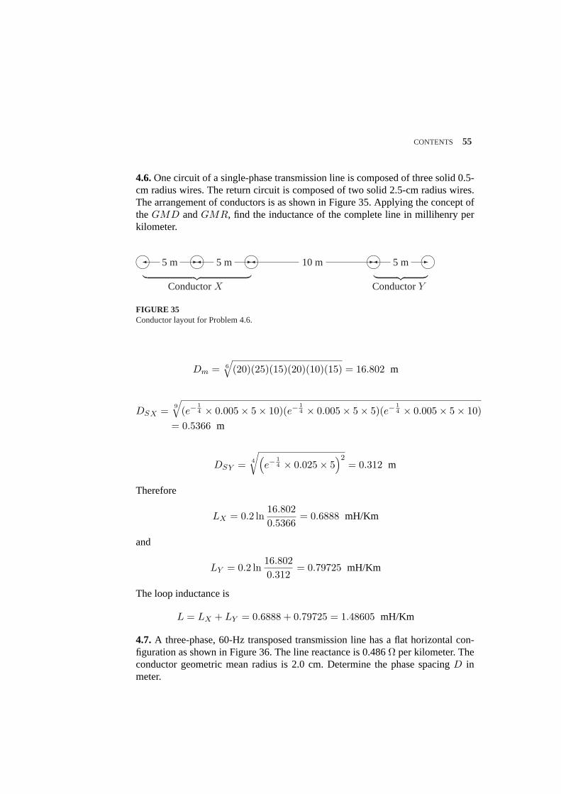
CONTENTS 55
4.6.One circuit of a single-phase transmission line is composed of three solid 0.5-cm radius wires. The return circuit is composed of two solid 2.5-cm radius wires.The arrangement of conductors is as shown in Figure 35. Applying the concept oftheGMD andGMR, find the inductance of the complete line in millihenry perkilometer.
m m m m m¾ -¾ -¾ -¾ -5 m 5 m 10 m 5 m︸ ︷︷ ︸
ConductorX︸ ︷︷ ︸ConductorY
FIGURE 35Conductor layout for Problem 4.6.
Dm = 6
√(20)(25)(15)(20)(10)(15) = 16.802 m
DSX = 9√
(e−14 × 0.005× 5× 10)(e−
14 × 0.005× 5× 5)(e−
14 × 0.005× 5× 10)
= 0.5366 m
DSY = 4
√(e−
14 × 0.025× 5
)2= 0.312 m
Therefore
LX = 0.2 ln16.8020.5366
= 0.6888 mH/Km
and
LY = 0.2 ln16.8020.312
= 0.79725 mH/Km
The loop inductance is
L = LX + LY = 0.6888 + 0.79725 = 1.48605 mH/Km
4.7. A three-phase, 60-Hz transposed transmission line has a flat horizontal con-figuration as shown in Figure 36. The line reactance is 0.486Ω per kilometer. Theconductor geometric mean radius is 2.0 cm. Determine the phase spacingD inmeter.
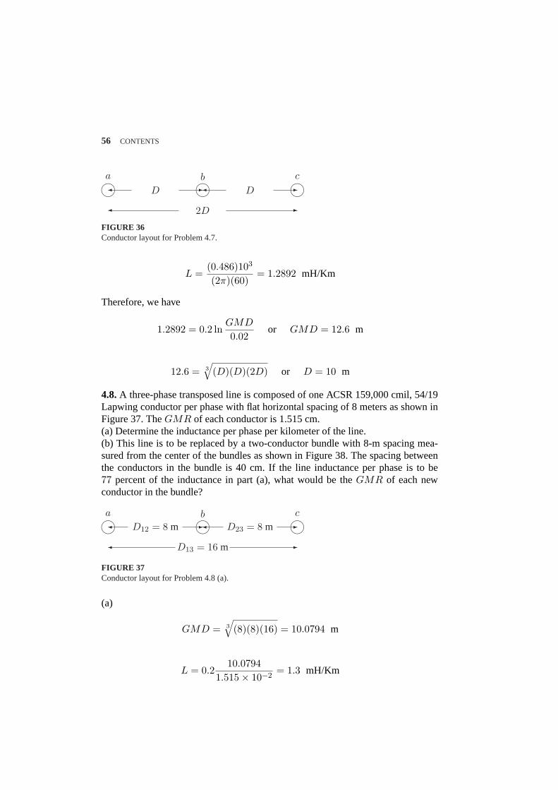
56 CONTENTS
m m m¾ -¾ -
¾ -
D D
2D
a b c
FIGURE 36Conductor layout for Problem 4.7.
L =(0.486)103
(2π)(60)= 1.2892 mH/Km
Therefore, we have
1.2892 = 0.2 lnGMD
0.02or GMD = 12.6 m
12.6 = 3
√(D)(D)(2D) or D = 10 m
4.8.A three-phase transposed line is composed of one ACSR 159,000 cmil, 54/19Lapwing conductor per phase with flat horizontal spacing of 8 meters as shown inFigure 37. TheGMR of each conductor is 1.515 cm.(a) Determine the inductance per phase per kilometer of the line.(b) This line is to be replaced by a two-conductor bundle with 8-m spacing mea-sured from the center of the bundles as shown in Figure 38. The spacing betweenthe conductors in the bundle is 40 cm. If the line inductance per phase is to be77 percent of the inductance in part (a), what would be theGMR of each newconductor in the bundle?
m m m¾ -¾ -
¾ -
D12 = 8 m D23 = 8 m
D13 = 16 m
a b c
FIGURE 37Conductor layout for Problem 4.8 (a).
(a)
GMD = 3
√(8)(8)(16) = 10.0794 m
L = 0.210.0794
1.515× 10−2= 1.3 mH/Km
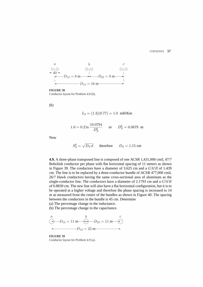
CONTENTS 57
f f f f f f
¾ -¾ -
¾ -
- ¾40D12 = 8 m D23 = 8 m
D13 = 16 m
a b c.............
.............
.............
.....
.............
.............
.....
.............
.............
.............
.............
.........
FIGURE 38Conductor layout for Problem 4.8 (b).
(b)
L2 = (1.3)(0.77) = 1.0 mH/Km
1.0 = 0.2 ln10.0794
DbS
or DbS = 0.0679 m
Now
SbS =
√DS d therefore DS = 1.15 cm
4.9.A three-phase transposed line is composed of one ACSR 1,431,000 cmil, 47/7Bobolink conductor per phase with flat horizontal spacing of 11 meters as shownin Figure 39. The conductors have a diameter of 3.625 cm and aGMR of 1.439cm. The line is to be replaced by a three-conductor bundle of ACSR 477,000 cmil,26/7 Hawk conductors having the same cross-sectional area of aluminum as thesingle-conductor line. The conductors have a diameter of 2.1793 cm and aGMRof 0.8839 cm. The new line will also have a flat horizontal configuration, but it is tobe operated at a higher voltage and therefore the phase spacing is increased to 14m as measured from the center of the bundles as shown in Figure 40. The spacingbetween the conductors in the bundle is 45 cm. Determine(a) The percentage change in the inductance.(b) The percentage change in the capacitance.
m m m¾ -¾ -
¾ -
D12 = 11 m D23 = 11 m
D13 = 22 m
a b c
FIGURE 39Conductor layout for Problem 4.9 (a).
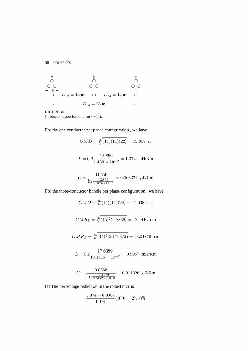
58 CONTENTS
f ff
f ff
f ff
¾ -¾ -
¾ -
- ¾45D12 = 14 m D23 = 14 m
D13 = 28 m
a b c
.............
.............
.............
.....
.............
.............
.....
.............
.............
.............
.............
.........
FIGURE 40Conductor layout for Problem 4.9 (b).
For the one conductor per phase configuration , we have
GMD = 3
√(11)(11)(22) = 13.859 m
L = 0.213.859
1.439× 10−2= 1.374 mH/Km
C =0.0556
ln 13.8591.8125×10−2
= 0.008374 µF/Km
For the three-conductor bundle per phase configuration , we have
GMD = 3
√(14)(14)(28) = 17.6389 m
GMRL = 3
√(45)2(0.8839) = 12.1416 cm
GMRC = 3
√(45)2(2.1793/2) = 13.01879 cm
L = 0.217.6389
12.1416× 10−2= 0.9957 mH/Km
C =0.0556
ln 17.638913.01879×10−2
= 0.011326 µF/Km
(a) The percentage reduction in the inductance is
1.374− 0.99571.374
(100) = 27.53%
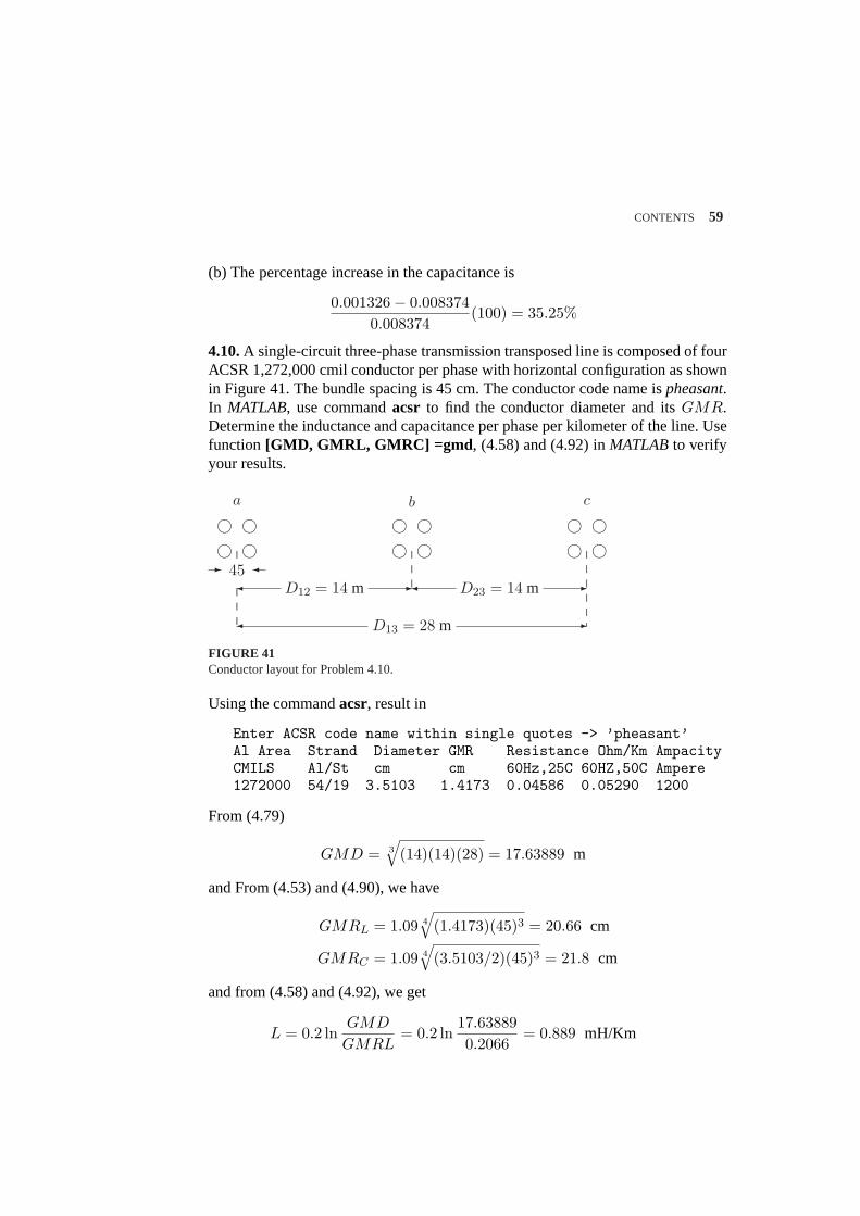
CONTENTS 59
(b) The percentage increase in the capacitance is
0.001326− 0.0083740.008374
(100) = 35.25%
4.10.A single-circuit three-phase transmission transposed line is composed of fourACSR 1,272,000 cmil conductor per phase with horizontal configuration as shownin Figure 41. The bundle spacing is 45 cm. The conductor code name ispheasant.In MATLAB, use commandacsr to find the conductor diameter and itsGMR.Determine the inductance and capacitance per phase per kilometer of the line. Usefunction [GMD, GMRL, GMRC] =gmd , (4.58) and (4.92) inMATLABto verifyyour results.
h hh h
h hh h
h hh h
¾ -¾ -
¾ -
- ¾45D12 = 14 m D23 = 14 m
D13 = 28 m
a b c
.............
.............
.............
.............
.............
.............
.............
.............
.............
.............
.............
.............
......
FIGURE 41Conductor layout for Problem 4.10.
Using the commandacsr, result in
Enter ACSR code name within single quotes -> ’pheasant’Al Area Strand Diameter GMR Resistance Ohm/Km AmpacityCMILS Al/St cm cm 60Hz,25C 60HZ,50C Ampere1272000 54/19 3.5103 1.4173 0.04586 0.05290 1200
From (4.79)
GMD = 3
√(14)(14)(28) = 17.63889 m
and From (4.53) and (4.90), we have
GMRL = 1.09 4
√(1.4173)(45)3 = 20.66 cm
GMRC = 1.09 4
√(3.5103/2)(45)3 = 21.8 cm
and from (4.58) and (4.92), we get
L = 0.2 lnGMD
GMRL= 0.2 ln
17.638890.2066
= 0.889 mH/Km
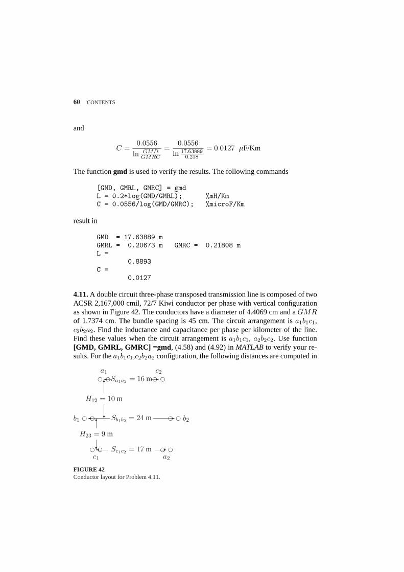
60 CONTENTS
and
C =0.0556
ln GMDGMRC
=0.0556
ln 17.638890.218
= 0.0127 µF/Km
The functiongmd is used to verify the results. The following commands
[GMD, GMRL, GMRC] = gmdL = 0.2*log(GMD/GMRL); %mH/KmC = 0.0556/log(GMD/GMRC); %microF/Km
result in
GMD = 17.63889 mGMRL = 0.20673 m GMRC = 0.21808 mL =
0.8893C =
0.0127
4.11.A double circuit three-phase transposed transmission line is composed of twoACSR 2,167,000 cmil, 72/7 Kiwi conductor per phase with vertical configurationas shown in Figure 42. The conductors have a diameter of 4.4069 cm and aGMRof 1.7374 cm. The bundle spacing is 45 cm. The circuit arrangement isa1b1c1,c2b2a2. Find the inductance and capacitance per phase per kilometer of the line.Find these values when the circuit arrangement isa1b1c1, a2b2c2. Use function[GMD, GMRL, GMRC] =gmd , (4.58) and (4.92) inMATLABto verify your re-sults. For thea1b1c1,c2b2a2 configuration, the following distances are computed in
ee ee
e e ee
e e eea1
b1
c1
c2
b2
a2
¾ -
¾ -
¾ -6
?6
?
Sa1a2 = 16 m
Sb1b2 = 24 m
Sc1c2 = 17 m
H12 = 10 m
H23 = 9 m
FIGURE 42Conductor layout for Problem 4.11.
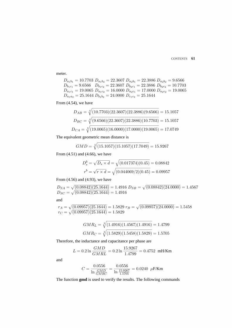
CONTENTS 61
meter.
Da1b1 = 10.7703 Da1b2 = 22.3607 Da2b1 = 22.3886 Da2b2 = 9.6566Db1c1 = 9.6566 Db1c2 = 22.3607 Db2c1 = 22.3886 Db2c2 = 10.7703Da1c1 = 19.0065 Da1c2 = 16.0000 Da2c1 = 17.0000 Da2c2 = 19.0065Da1a2 = 25.1644 Db1b2 = 24.0000 Dc1c2 = 25.1644
From (4.54), we have
DAB = 4
√(10.7703)(22.3607)(22.3886)(9.6566) = 15.1057
DBC = 4
√(9.6566)(22.3607)(22.3886)(10.7703) = 15.1057
DCA = 4
√(19.0065)(16.0000)(17.0000)(19.0065) = 17.0749
The equivalent geometric mean distance is
GMD = 3
√(15.1057)(15.1057)(17.7049) = 15.9267
From (4.51) and (4.66), we have
Dbs =
√Ds × d =
√(0.017374)(0.45) = 0.08842
rb =√
r × d =√
(0.044069/2)(0.45) = 0.09957
From (4.56) and (4.93), we have
DSA =√
(0.08842)(25.1644) = 1.4916 DSB =√
(0.08842)(24.0000) = 1.4567DSC =
√(0.08842)(25.1644) = 1.4916
and
rA =√
(0.09957)(25.1644) = 1.5829 rB =√
(0.09957)(24.0000) = 1.5458rC =
√(0.09957)(25.1644) = 1.5829
GMRL = 3
√(1.4916)(1.4567)(1.4916) = 1.4799
GMRC = 3
√(1.5829)(1.5458)(1.5829) = 1.5705
Therefore, the inductance and capacitance per phase are
L = 0.2 lnGMD
GMRL= 0.2 ln
15.92671.4799
= 0.4752 mH/Km
and
C =0.0556
ln GMDGMRC
=0.0556
ln 15.92671.5705
= 0.0240 µF/Km
The functiongmd is used to verify the results. The following commands
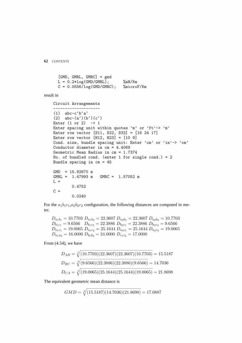
62 CONTENTS
[GMD, GMRL, GMRC] = gmdL = 0.2*log(GMD/GMRL); %mH/KmC = 0.0556/log(GMD/GMRC); %microF/Km
result in
Circuit Arrangements--------------------(1) abc-c‘b‘a‘(2) abc-(a‘)(b‘)(c‘)Enter (1 or 2) -> 1Enter spacing unit within quotes ’m’ or ’ft’-> ’m’Enter row vector [S11, S22, S33] = [16 24 17]Enter row vector [H12, H23] = [10 9]Cond. size, bundle spacing unit: Enter ’cm’ or ’in’-> ’cm’Conductor diameter in cm = 4.4069Geometric Mean Radius in cm = 1.7374No. of bundled cond. (enter 1 for single cond.) = 2Bundle spacing in cm = 45
GMD = 15.92670 mGMRL = 1.47993 m GMRC = 1.57052 mL =
0.4752C =
0.0240
For thea1b1c1,a2b2c2 configuration, the following distances are computed in me-ter.
Da1b1 = 10.7703 Da1b2 = 22.3607 Da2b1 = 22.3607 Da2b2 = 10.7703Db1c1 = 9.6566 Db1c2 = 22.3886 Db2c1 = 22.3886 Db2c2 = 9.6566Da1c1 = 19.0065 Da1c2 = 25.1644 Da2c1 = 25.1644 Da2c2 = 19.0065Da1a2 = 16.0000 Db1b2 = 24.0000 Dc1c2 = 17.0000
From (4.54), we have
DAB = 4
√(10.7703)(22.3607)(22.3607)(10.7703) = 15.5187
DBC = 4
√(9.6566)(22.3886)(22.3886)(9.6566) = 14.7036
DCA = 4
√(19.0065)(25.1644)(25.1644)(19.0065) = 21.8698
The equivalent geometric mean distance is
GMD = 3
√(15.5187)(14.7036)(21.8698) = 17.0887
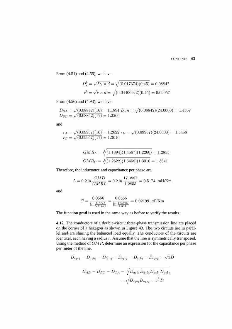
CONTENTS 63
From (4.51) and (4.66), we have
Dbs =
√Ds × d =
√(0.017374)(0.45) = 0.08842
rb =√
r × d =√
(0.044069/2)(0.45) = 0.09957
From (4.56) and (4.93), we have
DSA =√
(0.08842)(16) = 1.1894 DSB =√
(0.08842)(24.0000) = 1.4567DSC =
√(0.08842)(17) = 1.2260
and
rA =√
(0.09957)(16) = 1.2622 rB =√
(0.09957)(24.0000) = 1.5458rC =
√(0.09957)(17) = 1.3010
GMRL = 3
√(1.1894)(1.4567)(1.2260) = 1.2855
GMRC = 3
√(1.2622)(1.5458)(1.3010 = 1.3641
Therefore, the inductance and capacitance per phase are
L = 0.2 lnGMD
GMRL= 0.2 ln
17.08871.2855
= 0.5174 mH/Km
and
C =0.0556
ln GMDGMRC
=0.0556
ln 17.08871.3641
= 0.02199 µF/Km
The functiongmd is used in the same way as before to verify the results.
4.12.The conductors of a double-circuit three-phase transmission line are placedon the corner of a hexagon as shown in Figure 43. The two circuits are in paral-lel and are sharing the balanced load equally. The conductors of the circuits areidentical, each having a radiusr. Assume that the line is symmetrically transposed.Using the method ofGMR, determine an expression for the capacitance per phaseper meter of the line.
Da1c1 = Da1b2 = Db1a2 = Db1c2 = Dc1b2 = Dc2a2 =√
3D
DAB = DBC = DCA = 4
√Da1b1Da1b2Da2b1Da2b2
=√
Da1b1Da1b2 = 314 D
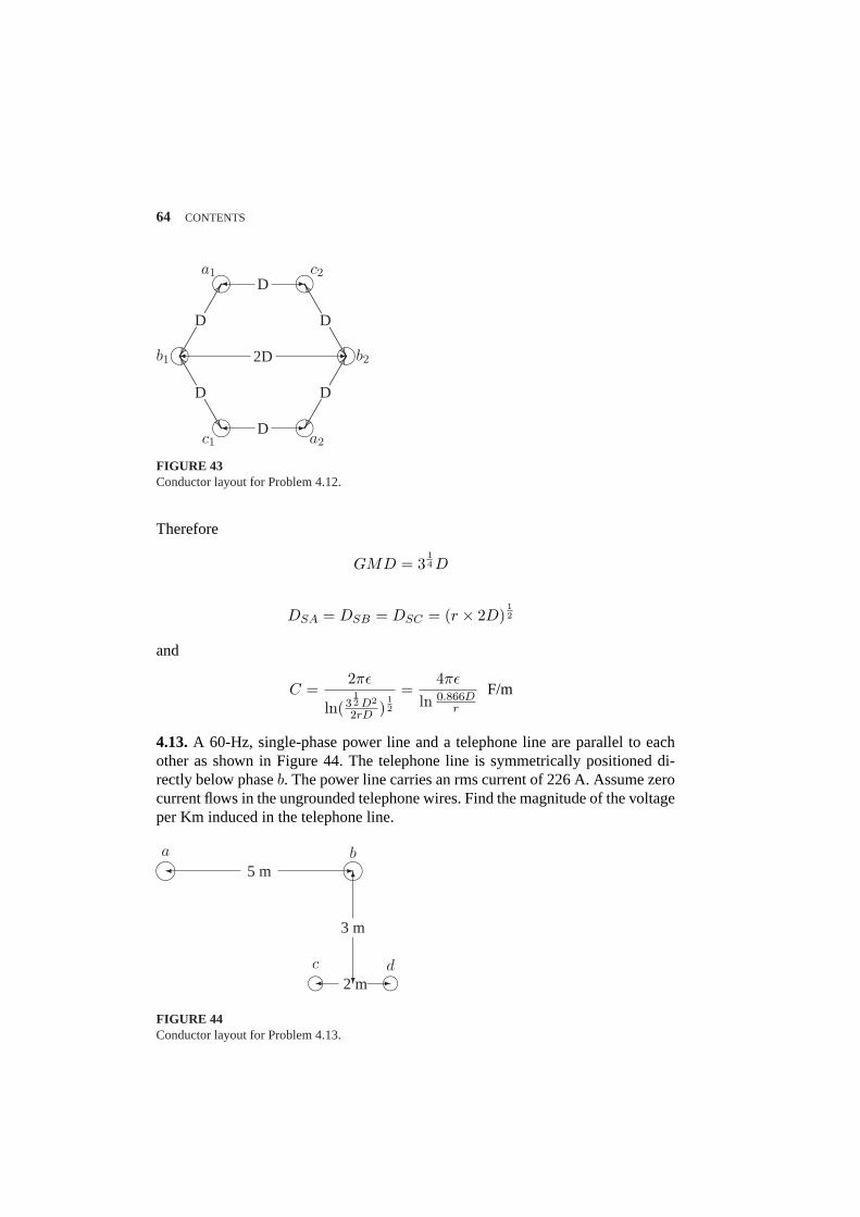
64 CONTENTS
k k
k k
k k¾ -
¾ -
¾ -
D
2D
D
..........................................................................................
D..........................................................................................
..........................................................................................
D..........................................................................................
..........................................................................................
D..........................................................................................
..........................................................................................
D..........................................................................................
a1 c2
b1 b2
c1 a2
FIGURE 43Conductor layout for Problem 4.12.
Therefore
GMD = 314 D
DSA = DSB = DSC = (r × 2D)12
and
C =2πε
ln(312 D2
2rD )12
=4πε
ln 0.866Dr
F/m
4.13.A 60-Hz, single-phase power line and a telephone line are parallel to eachother as shown in Figure 44. The telephone line is symmetrically positioned di-rectly below phaseb. The power line carries an rms current of 226 A. Assume zerocurrent flows in the ungrounded telephone wires. Find the magnitude of the voltageper Km induced in the telephone line.
l l
i i
¾ -
¾ -
6
?
5 m
2 m
3 m
a b
c d
FIGURE 44Conductor layout for Problem 4.13.
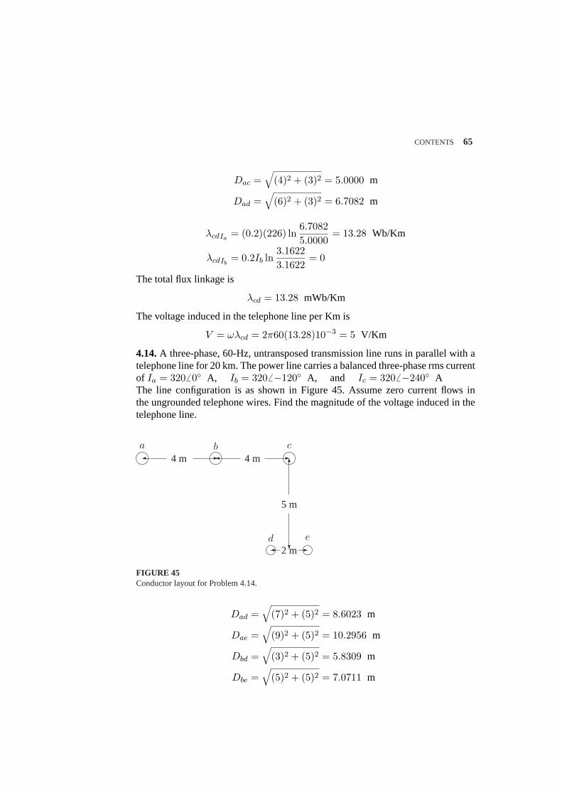
CONTENTS 65
Dac =√
(4)2 + (3)2 = 5.0000 m
Dad =√
(6)2 + (3)2 = 6.7082 m
λcdIa= (0.2)(226) ln
6.70825.0000
= 13.28 Wb/Km
λcdIb= 0.2Ib ln
3.16223.1622
= 0
The total flux linkage is
λcd = 13.28 mWb/Km
The voltage induced in the telephone line per Km is
V = ωλcd = 2π60(13.28)10−3 = 5 V/Km
4.14.A three-phase, 60-Hz, untransposed transmission line runs in parallel with atelephone line for 20 km. The power line carries a balanced three-phase rms currentof Ia = 3206 0 A, Ib = 3206 −120 A, and Ic = 3206 −240 AThe line configuration is as shown in Figure 45. Assume zero current flows inthe ungrounded telephone wires. Find the magnitude of the voltage induced in thetelephone line.
l l l
i i
¾ -¾ -6
?¾ -
4 m 4 m
2 m
5 m
a b c
d e
FIGURE 45Conductor layout for Problem 4.14.
Dad =√
(7)2 + (5)2 = 8.6023 m
Dae =√
(9)2 + (5)2 = 10.2956 m
Dbd =√
(3)2 + (5)2 = 5.8309 m
Dbe =√
(5)2 + (5)2 = 7.0711 m
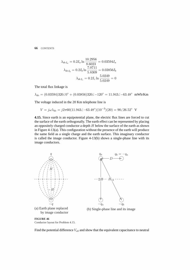
66 CONTENTS
λdeIa= 0.2Ia ln
10.29568.6023
= 0.03594Ia
λdeIb= 0.2Ib ln
7.07115.8309
= 0.03856Ib
λdeIc= 0.2Ic ln
5.02495.0249
= 0
The total flux linkage is
λde = (0.03594)3206 0 + (0.03856)3206 −120 = 11.9436 −63.48 mWb/Km
The voltage induced in the 20 Km telephone line is
V = jωλde = j2π60(11.9436 −63.48)(10−3)(20) = 906 26.52 V
4.15.Since earth is an equipotential plane, the electric flux lines are forced to cutthe surface of the earth orthogonally. The earth effect can be represented by placingan oppositely charged conductor a depthH below the surface of the earth as shownin Figure 4-13(a). This configuration without the presence of the earth will producethe same field as a single charge and the earth surface. This imaginary conductoris called the image conductor. Figure 4-13(b) shows a single-phase line with itsimage conductors.
l
l
l l
l l
........
........
........
........
........
........
........
........
........
........
........
........
........
........
........
........
........
........
...................
................
...........................................................................................................................................................
........
........
........
....................................................................................................................................................................................................
....................................................................................................................................................................................................
.................................................................................................. .................................................................................. ................
........
................................................................................................ .....
........
........................................................................................
........
........
..........................................................................
........
........................................................................................
.............
........
........................................................................................
........
........
..........................................................................
........
........................................
................
................
................
.............
........
................................................
................
................
........
........
........
..........................................................................
........
.....................................................................................................
........
........................................................................................
........
........
..........................................................................
........ ........ ........ ........ ........ ........ ........ ........ ........ ........ ........ ........ ........ ........ ........ ........ ........ ......
........
........
........
........
......
........
........
........
........
........
........
........
........
........
........
........
........
........
......
........ ........ ... ........ ........ ... ........ ........ ........ ........ ......
q
−q
H
−H
qa qb = −qa
−qa −qb
2H H12
D
(a) Earth plane replacedby image conductor
(b) Single-phase line and its image
FIGURE 46Conductor layout for Problem 4.15.
Find the potential differenceVab and show that the equivalent capacitance to neutral
CONTENTS 67
is given by
Can = Cbn =2πε
ln(
Dr
2HH12
)
Vab =1
2πε
[qa ln
D
r− qa ln
H12
2H+ qb ln
r
D− qb ln
2H
H12
]
Substituting forqb = −qa, results in
Vab =qa
πε
[ln
(D
r
2H
H12
)]
Cab =qa
Vab=
πε
ln(
Dr
2HH12
)
Therefore, the equivalent capacitance to neutral is
Can = Cbn = 2Cab =2πε
ln(
Dr
2HH12
)
CHAPTER 5 PROBLEMS
5.1.A 69-kV, three-phase short transmission line is 16 km long. The line has a perphase series impedance of0.125 + j0.4375 Ω per km. Determine the sending endvoltage, voltage regulation, the sending end power, and the transmission efficiencywhen the line delivers
(a) 70 MVA, 0.8 lagging power factor at 64 kV.(b) 120 MW, unity power factor at 64 kV.
Uselineperf program to verify your results.
The line impedance is
Z = (0.125 + j0.4375)(16) = 2 + j7 Ω
The receiving end voltage per phase is
VR =646 0√
3= 36.95046 0 kV
(a) The complex power at the receiving end is
SR(3φ) = 706 cos−1 0.8 = 706 36.87 = 56 + j42 MVA
The current per phase is given by
IR =S∗R(3φ)
3V ∗R
=700006 − 36.87
3× 36.95046 0= 631.4776 − 36.87 A
68
CONTENTS 69
The sending end voltage is
VS = VR + ZIR = 36.95046 0 + (2 + j7)(631.4776 − 36.87)(10−3)= 40.7086 3.9137 kV
The sending end line-to-line voltage magnitude is
|VS(L−L)| =√
3 |VS | = 70.508 kV
The sending end power is
SS(3φ) = 3VSI∗S = 3× 40.7086 3.9137× 631.4776 36.87 × 10−3
= 58.393 MW + j50.374 Mvar
= 77.11856 40.7837 MVA
Voltage regulation is
PercentV R =70.508− 64
64× 100 = 10.169%
Transmission line efficiency is
η =PR(3φ)
PS(3φ)=
5658.393
× 100 = 95.90%
(b) The complex power at the receiving end is
SR(3φ) = 1206 0 = 120 + j0 MVA
The current per phase is given by
IR =S∗R(3φ)
3V ∗R
=1200006 0
3× 36.95046 0= 1082.53 6 0 A
The sending end voltage is
VS = VR + ZIR = 36.95046 0 + (2 + j7)(1082.53 6 0)(10−3)= 39.84276 10.9639 kV
The sending end line-to-line voltage magnitude is
|VS(L−L)| =√
3 |VS | = 69.0096 kV
70 CONTENTS
The sending end power is
SS(3φ) = 3VSI∗S = 3× 39.84276 10.9639× 1082.53 6 0 × 10−3
= 127.031 MW + j24.609 Mvar
= 129.3936 10.9639 MVA
Voltage regulation is
PercentV R =69.0096− 64
64× 100 = 7.8275%
Transmission line efficiency is
η =PR(3φ)
PS(3φ)=
120127.031
× 100 = 94.465%
The above computations are performed efficiently using thelineperf program.
The command:
lineperf
displays the following menu
Type of parameters for input SelectParameters per unit lengthr (Ω), g (Siemens), L (mH), C (µF) 1
Complex z and y per unit lengthr + j*x (Ω), g + j*b (Siemens) 2
Nominal π or Eq. π model 3
A, B, C, D constants 4
Conductor configuration and dimension 5
To quit 0Select number of menu → 2Enter line length = 16Enter frequency in Hz = 60Enter series impedance r + j*x in ohm per unit lengthz = 0.125+j*0.4375Enter shunt admittance g + j*b in siemens per unit lengthy = 0+j*0
CONTENTS 71
Short line modelZ = 2 + j 7 ohms
ABCD =[
1 + j0 2 + j70 + j0 1 + j0
]
Transmission line performanceAnalysis Select
To calculate sending end quantitiesfor specified receiving end MW, Mvar 1
To calculate receiving end quantitiesfor specified sending end MW, Mvar 2
To calculate sending end quantitieswhen load impedance is specified 3
Open-end line and reactive compensation 4
Short-circuited line 5
Capacitive compensation 6
Receiving end circle diagram 7
Loadability curve and voltage profile 8
To quit 0
Select number of menu → 1
Enter receiving end line-line voltage kV = 64Enter receiving end voltage phase angle = 0Enter receiving end 3-phase power MW = 56Enter receiving end 3-phase reactive power(+ for lagging and - for leading power factor) Mvar = 42
Line performance for specified receiving end quantities
Vr = 64 kV (L-L) at 0Pr = 56 MW Qr = 42 Mvar
72 CONTENTS
Ir = 631.477 A at -36.8699 PFr = 0.8 laggingVs = 70.5082 kV (L-L) at 3.91374Is = 631.477 A at -36.8699 PFs = 0.757182 laggingPs = 58.393 MW Qs = 50.374 MvarPL = 2.393 MW QL = 8.374 MvarPercent Voltage Regulation = 10.169Transmission line efficiency = 95.9026
At the end of this analysis thelistmenu (Analysis Menu) is displayed. Selectingoption 1 and entering data for part (b), will result in
Line performance for specified receiving end quantities
Vr = 64 kV (L-L) at 0Pr = 120 MW Qr = 0 MvarIr = 1082.53 A at 0 PFr = 1Vs = 69.0096 kV (L-L) at 10.9639Is = 1082.53 A at 0 PFs = 0.981747Ps = 127.031 MW Qs = 24.069 MvarPL = 7.031 MW QL = 24.069 MvarPercent Voltage Regulation = 7.82754Transmission line efficiency = 94.4649
5.2.Shunt capacitors are installed at the receiving end to improve the line perfor-mance of Problem 5.1. The line delivers 70 MVA, 0.8 lagging power factor at 64kV. Determine the total Mvar and the capacitance per phase of the Y-connectedcapacitors when the sending end voltage is
(a) 69 kV.(b) 64 kV.
Hint: Use (5.85) and (5.86) to compute the power angleδ and the receivingend reactive power.(c) Uselineperf to obtain the compensated line performance.
The complex load at the receiving end is
SR(3φ) = 70 6 cos−1 0.8 = 56 MW + j42 Mvar
Z = 2 + j7 = 7.286 74.0546
(a) ForVR(LL) = 69 kV, from (5.85), we have
56 =(69)(64)
7.28cos(74.0564− δ)− (1.0)(64)2
7.28cos 74.0546
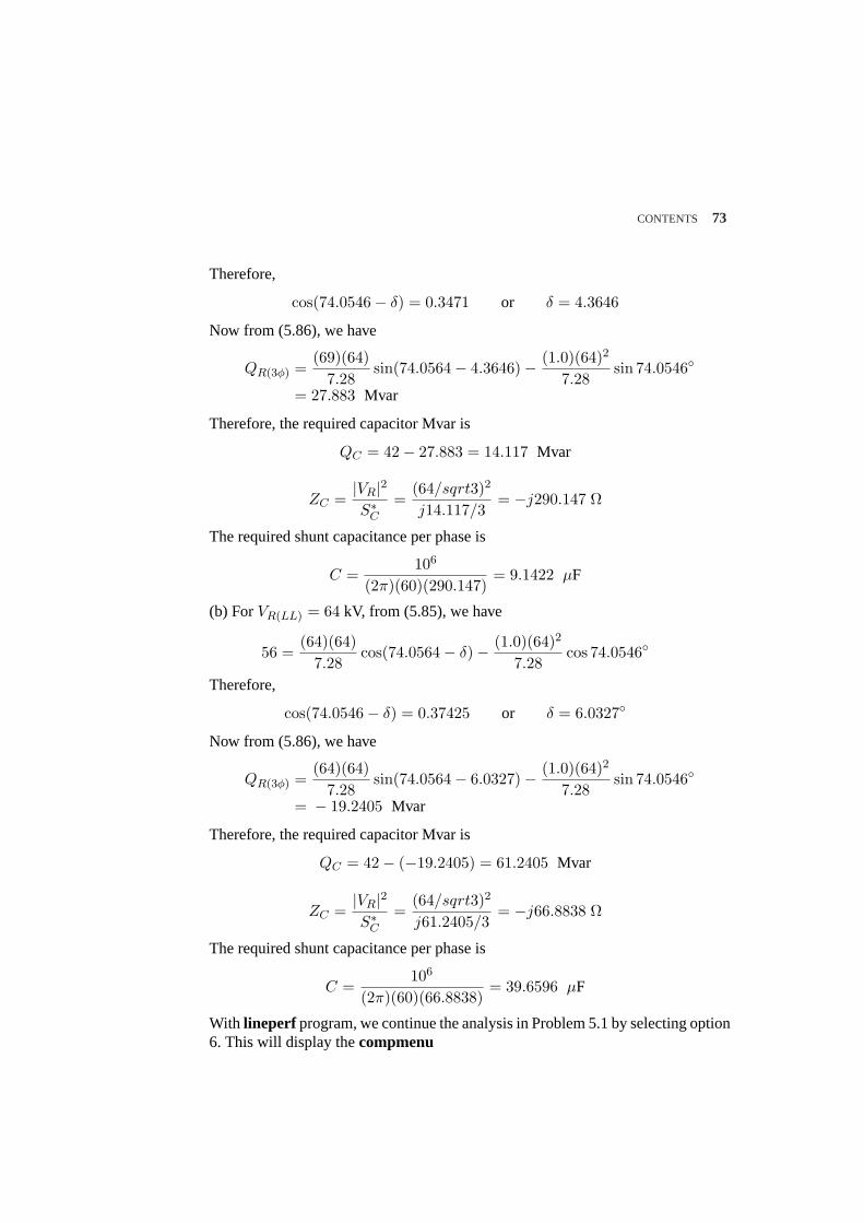
CONTENTS 73
Therefore,
cos(74.0546− δ) = 0.3471 or δ = 4.3646
Now from (5.86), we have
QR(3φ) =(69)(64)
7.28sin(74.0564− 4.3646)− (1.0)(64)2
7.28sin 74.0546
= 27.883 Mvar
Therefore, the required capacitor Mvar is
QC = 42− 27.883 = 14.117 Mvar
ZC =|VR|2S∗C
=(64/sqrt3)2
j14.117/3= −j290.147 Ω
The required shunt capacitance per phase is
C =106
(2π)(60)(290.147)= 9.1422 µF
(b) ForVR(LL) = 64 kV, from (5.85), we have
56 =(64)(64)
7.28cos(74.0564− δ)− (1.0)(64)2
7.28cos 74.0546
Therefore,
cos(74.0546− δ) = 0.37425 or δ = 6.0327
Now from (5.86), we have
QR(3φ) =(64)(64)
7.28sin(74.0564− 6.0327)− (1.0)(64)2
7.28sin 74.0546
= − 19.2405 Mvar
Therefore, the required capacitor Mvar is
QC = 42− (−19.2405) = 61.2405 Mvar
ZC =|VR|2S∗C
=(64/sqrt3)2
j61.2405/3= −j66.8838 Ω
The required shunt capacitance per phase is
C =106
(2π)(60)(66.8838)= 39.6596 µF
With lineperf program, we continue the analysis in Problem 5.1 by selecting option6. This will display thecompmenu
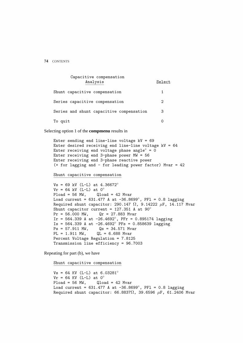
74 CONTENTS
Capacitive compensationAnalysis Select
Shunt capacitive compensation 1
Series capacitive compensation 2
Series and shunt capacitive compensation 3
To quit 0
Selecting option 1 of thecompmenuresults in
Enter sending end line-line voltage kV = 69Enter desired receiving end line-line voltage kV = 64Enter receiving end voltage phase angle = 0Enter receiving end 3-phase power MW = 56Enter receiving end 3-phase reactive power(+ for lagging and - for leading power factor) Mvar = 42
Shunt capacitive compensation
Vs = 69 kV (L-L) at 4.36672Vr = 64 kV (L-L) at 0Pload = 56 MW, Qload = 42 MvarLoad current = 631.477 A at -36.8699, PFl = 0.8 laggingRequired shunt capacitor: 290.147 Ω, 9.14222 µF, 14.117 MvarShunt capacitor current = 127.351 A at 90Pr = 56.000 MW, Qr = 27.883 MvarIr = 564.339 A at -26.4692, PFr = 0.895174 laggingIs = 564.339 A at -26.4692 PFs = 0.858639 laggingPs = 57.911 MW, Qs = 34.571 MvarPL = 1.911 MW, QL = 6.688 MvarPercent Voltage Regulation = 7.8125Transmission line efficiency = 96.7003
Repeating for part (b), we have
Shunt capacitive compensation
Vs = 64 KV (L-L) at 6.03281Vr = 64 KV (L-L) at 0Pload = 56 MW, Qload = 42 MvarLoad current = 631.477 A at -36.8699, PFl = 0.8 laggingRequired shunt capacitor: 66.8837Ω, 39.6596 µF, 61.2406 Mvar
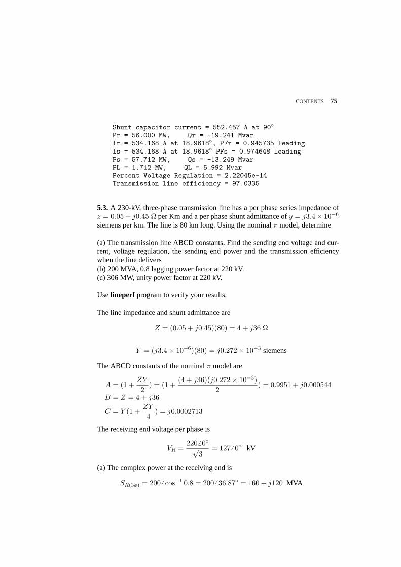
CONTENTS 75
Shunt capacitor current = 552.457 A at 90Pr = 56.000 MW, Qr = -19.241 MvarIr = 534.168 A at 18.9618, PFr = 0.945735 leadingIs = 534.168 A at 18.9618 PFs = 0.974648 leadingPs = 57.712 MW, Qs = -13.249 MvarPL = 1.712 MW, QL = 5.992 MvarPercent Voltage Regulation = 2.22045e-14Transmission line efficiency = 97.0335
5.3.A 230-kV, three-phase transmission line has a per phase series impedance ofz = 0.05 + j0.45 Ω per Km and a per phase shunt admittance ofy = j3.4× 10−6
siemens per km. The line is 80 km long. Using the nominalπ model, determine
(a) The transmission line ABCD constants. Find the sending end voltage and cur-rent, voltage regulation, the sending end power and the transmission efficiencywhen the line delivers(b) 200 MVA, 0.8 lagging power factor at 220 kV.(c) 306 MW, unity power factor at 220 kV.
Uselineperf program to verify your results.
The line impedance and shunt admittance are
Z = (0.05 + j0.45)(80) = 4 + j36 Ω
Y = (j3.4× 10−6)(80) = j0.272× 10−3 siemens
The ABCD constants of the nominalπ model are
A = (1 +ZY
2) = (1 +
(4 + j36)(j0.272× 10−3)2
) = 0.9951 + j0.000544
B = Z = 4 + j36
C = Y (1 +ZY
4) = j0.0002713
The receiving end voltage per phase is
VR =2206 0√
3= 1276 0 kV
(a) The complex power at the receiving end is
SR(3φ) = 2006 cos−1 0.8 = 2006 36.87 = 160 + j120 MVA
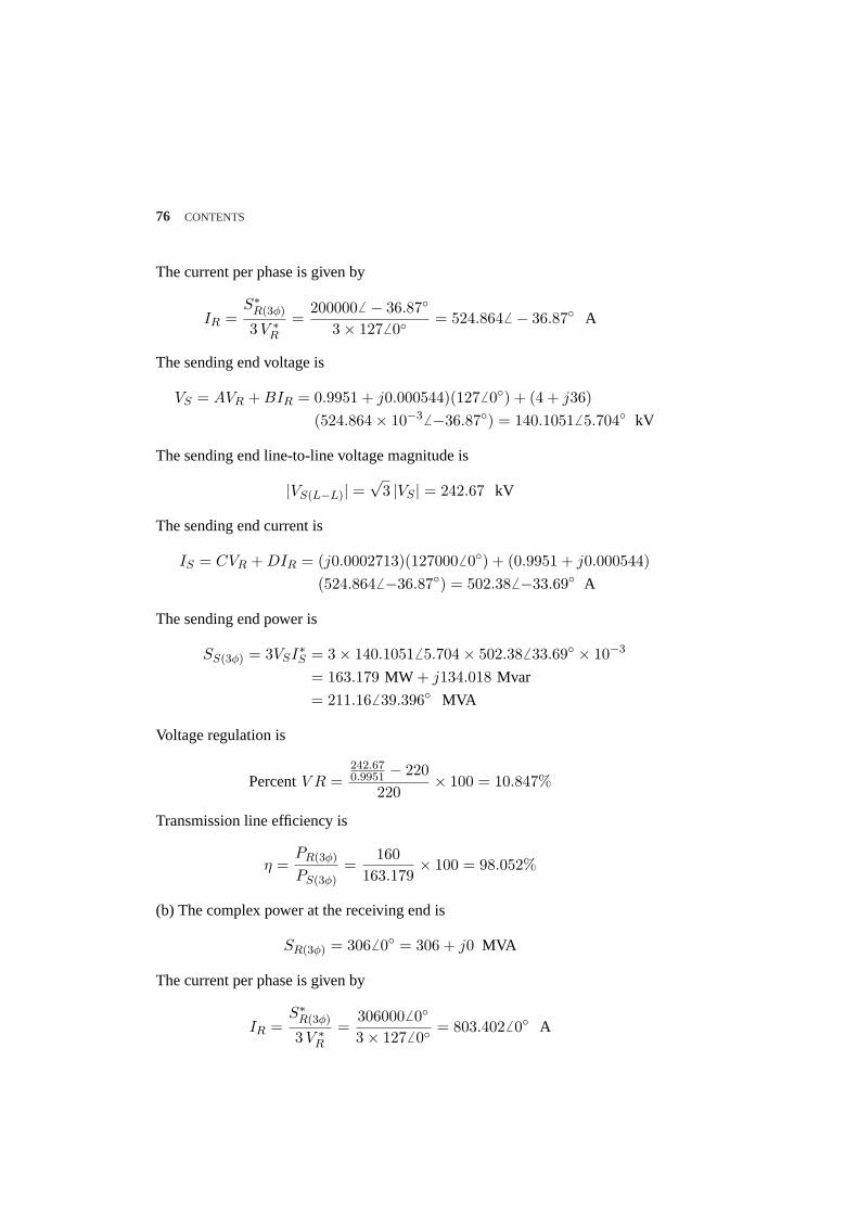
76 CONTENTS
The current per phase is given by
IR =S∗R(3φ)
3V ∗R
=2000006 − 36.87
3× 1276 0= 524.8646 − 36.87 A
The sending end voltage is
VS = AVR + BIR = 0.9951 + j0.000544)(1276 0) + (4 + j36)(524.864× 10⁻³ 6 −36.87) = 140.10516 5.704 kV
The sending end line-to-line voltage magnitude is
|VS(L−L)| =√
3 |VS | = 242.67 kV
The sending end current is
IS = CVR + DIR = (j0.0002713)(1270006 0) + (0.9951 + j0.000544)(524.8646 −36.87) = 502.38 6 −33.69 A
The sending end power is
SS(3φ) = 3VSI∗S = 3× 140.10516 5.704× 502.386 33.69 × 10−3
= 163.179 MW + j134.018 Mvar
= 211.166 39.396 MVA
Voltage regulation is
PercentV R =242.670.9951 − 220
220× 100 = 10.847%
Transmission line efficiency is
η =PR(3φ)
PS(3φ)=
160163.179
× 100 = 98.052%
(b) The complex power at the receiving end is
SR(3φ) = 3066 0 = 306 + j0 MVA
The current per phase is given by
IR =S∗R(3φ)
3V ∗R
=3060006 0
3× 1276 0= 803.4026 0 A
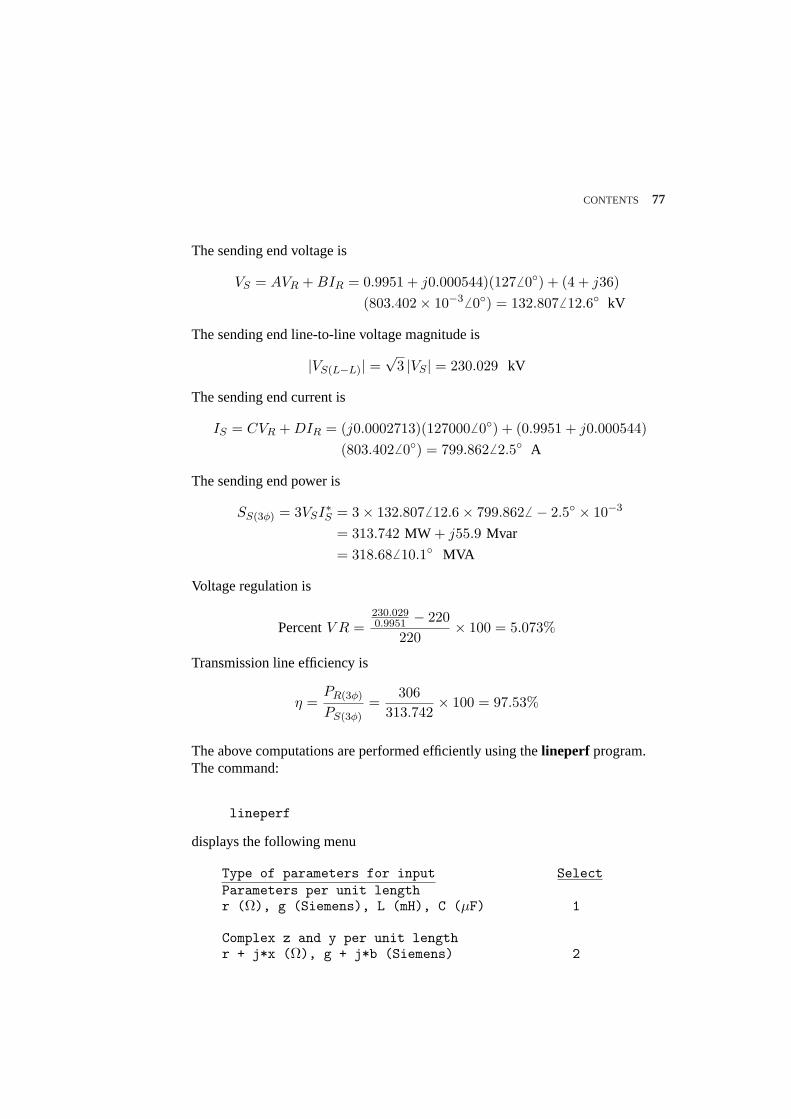
CONTENTS 77
The sending end voltage is
VS = AVR + BIR = 0.9951 + j0.000544)(1276 0) + (4 + j36)(803.402× 10⁻³ 6 0) = 132.8076 12.6 kV
The sending end line-to-line voltage magnitude is
|VS(L−L)| =√
3 |VS | = 230.029 kV
The sending end current is
IS = CVR + DIR = (j0.0002713)(1270006 0) + (0.9951 + j0.000544)(803.4026 0) = 799.8626 2.5 A
The sending end power is
SS(3φ) = 3VSI∗S = 3× 132.8076 12.6× 799.8626 − 2.5 × 10−3
= 313.742 MW + j55.9 Mvar
= 318.686 10.1 MVA
Voltage regulation is
PercentV R =230.0290.9951 − 220
220× 100 = 5.073%
Transmission line efficiency is
η =PR(3φ)
PS(3φ)=
306313.742
× 100 = 97.53%
The above computations are performed efficiently using thelineperf program.The command:
lineperf
displays the following menu
Type of parameters for input SelectParameters per unit lengthr (Ω), g (Siemens), L (mH), C (µF) 1
Complex z and y per unit lengthr + j*x (Ω), g + j*b (Siemens) 2
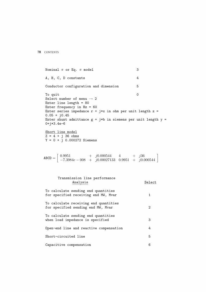
78 CONTENTS
Nominal π or Eq. π model 3
A, B, C, D constants 4
Conductor configuration and dimension 5
To quit 0Select number of menu → 2Enter line length = 80Enter frequency in Hz = 60Enter series impedance r + j*x in ohm per unit length z =0.05 + j0.45Enter shunt admittance g + j*b in siemens per unit length y =0+j*3.4e-6
Short line modelZ = 4 + j 36 ohmsY = 0 + j 0.000272 Siemens
ABCD =[
0.9951 + j0.000544 4 + j36−7.3984e− 008 + j0.00027133 0.9951 + j0.000544
]
Transmission line performanceAnalysis Select
To calculate sending end quantitiesfor specified receiving end MW, Mvar 1
To calculate receiving end quantitiesfor specified sending end MW, Mvar 2
To calculate sending end quantitieswhen load impedance is specified 3
Open-end line and reactive compensation 4
Short-circuited line 5
Capacitive compensation 6

CONTENTS 79
Receiving end circle diagram 7
Loadability curve and voltage profile 8
To quit 0
Select number of menu → 1
Enter receiving end line-line voltage kV = 220Enter receiving end voltage phase angle = 0Enter receiving end 3-phase power MW = 160Enter receiving end 3-phase reactive power(+ for lagging and - for leading power factor) Mvar = 120
Line performance for specified receiving end quantities
Vr = 220 kV (L-L) at 0Pr = 160 MW Qr = 120 MvarIr = 524.864 A at -36.8699 PFr = 0.8 laggingVs = 242.67 kV (L-L) at 5.7042Is = 502.381 A at -33.6919 PFs = 0.77277 laggingPs = 163.179 MW Qs = 134.018 MvarPL = 3.179 MW QL = 14.018 MvarPercent Voltage Regulation = 10.847Transmission line efficiency = 98.052
At the end of this analysis thelistmenu (Analysis Menu) is displayed. Selectingoption 1 and entering data for part (b), will result in
Line performance for specified receiving end quantities
Vr = 220 kV (L-L) at 0Pr = 306 MW Qr = 0 MvarIr = 803.042 A at 0 PFr = 1Vs = 230.029 kV (L-L) at 12.6033Is = 799.862 A at 2.5008 PFs = 0.984495Ps = 313.742 MW Qs = 55.900 MvarPL = 7.742 MW QL = 55.900 MvarPercent Voltage Regulation = 5.0732Transmission line efficiency = 97.532
5.4.Shunt capacitors are installed at the receiving end to improve the line perfor-mance of Problem 5.3. The line delivers 200 MVA, 0.8 lagging power factor at 220kV.
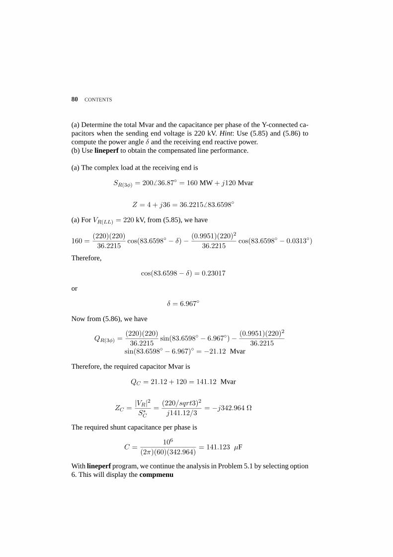
80 CONTENTS
(a) Determine the total Mvar and the capacitance per phase of the Y-connected ca-pacitors when the sending end voltage is 220 kV.Hint: Use (5.85) and (5.86) tocompute the power angleδ and the receiving end reactive power.(b) Uselineperf to obtain the compensated line performance.
(a) The complex load at the receiving end is
SR(3φ) = 2006 36.87 = 160 MW + j120 Mvar
Z = 4 + j36 = 36.22156 83.6598
(a) ForVR(LL) = 220 kV, from (5.85), we have
160 =(220)(220)36.2215
cos(83.6598 − δ)− (0.9951)(220)2
36.2215cos(83.6598 − 0.0313)
Therefore,
cos(83.6598− δ) = 0.23017
or
δ = 6.967
Now from (5.86), we have
QR(3φ) =(220)(220)36.2215
sin(83.6598 − 6.967)− (0.9951)(220)2
36.2215sin(83.6598 − 6.967) = −21.12 Mvar
Therefore, the required capacitor Mvar is
QC = 21.12 + 120 = 141.12 Mvar
ZC =|VR|2S∗C
=(220/sqrt3)2
j141.12/3= −j342.964 Ω
The required shunt capacitance per phase is
C =106
(2π)(60)(342.964)= 141.123 µF
With lineperf program, we continue the analysis in Problem 5.1 by selecting option6. This will display thecompmenu
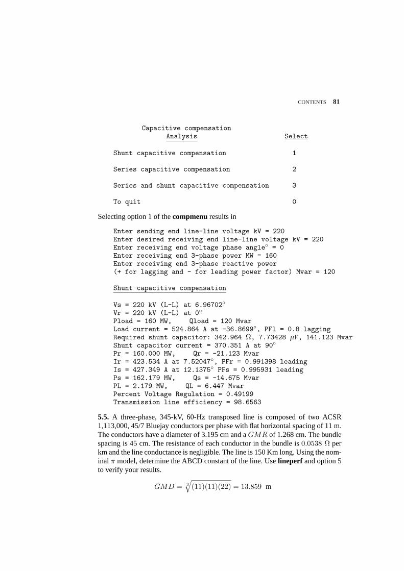
CONTENTS 81
Capacitive compensationAnalysis Select
Shunt capacitive compensation 1
Series capacitive compensation 2
Series and shunt capacitive compensation 3
To quit 0
Selecting option 1 of thecompmenuresults in
Enter sending end line-line voltage kV = 220Enter desired receiving end line-line voltage kV = 220Enter receiving end voltage phase angle = 0Enter receiving end 3-phase power MW = 160Enter receiving end 3-phase reactive power(+ for lagging and - for leading power factor) Mvar = 120
Shunt capacitive compensation
Vs = 220 kV (L-L) at 6.96702Vr = 220 kV (L-L) at 0Pload = 160 MW, Qload = 120 MvarLoad current = 524.864 A at -36.8699, PFl = 0.8 laggingRequired shunt capacitor: 342.964 Ω, 7.73428 µF, 141.123 MvarShunt capacitor current = 370.351 A at 90Pr = 160.000 MW, Qr = -21.123 MvarIr = 423.534 A at 7.52047, PFr = 0.991398 leadingIs = 427.349 A at 12.1375 PFs = 0.995931 leadingPs = 162.179 MW, Qs = -14.675 MvarPL = 2.179 MW, QL = 6.447 MvarPercent Voltage Regulation = 0.49199Transmission line efficiency = 98.6563
5.5. A three-phase, 345-kV, 60-Hz transposed line is composed of two ACSR1,113,000, 45/7 Bluejay conductors per phase with flat horizontal spacing of 11 m.The conductors have a diameter of 3.195 cm and aGMR of 1.268 cm. The bundlespacing is 45 cm. The resistance of each conductor in the bundle is0.0538 Ω perkm and the line conductance is negligible. The line is 150 Km long. Using the nom-inal π model, determine the ABCD constant of the line. Uselineperf and option 5to verify your results.
GMD = 3
√(11)(11)(22) = 13.859 m
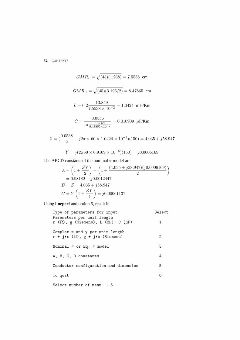
82 CONTENTS
GMRL =√
(45)(1.268) = 7.5538 cm
GMRC =√
(45)(3.195/2) = 8.47865 cm
L = 0.213.859
7.5538× 10−2= 1.0424 mH/Km
C =0.0556
ln 13.8598.47865×10−2
= 0.010909 µF/Km
Z = (0.0538
2+ j2π × 60× 1.0424× 10−3)(150) = 4.035 + j58.947
Y = j(2π60× 0.9109× 10−6)(150) = j0.0006169
The ABCD constants of the nominalπ model are
A =(
1 +ZY
2
)=
(1 +
(4.035 + j38.947)(j0.0006169)2
)
= 0.98182 + j0.0012447B = Z = 4.035 + j58.947
C = Y
(1 +
ZY
4
)= j0.00061137
Using lineperf and option 5, result in
Type of parameters for input SelectParameters per unit lengthr (Ω), g (Siemens), L (mH), C (µF) 1
Complex z and y per unit lengthr + j*x (Ω), g + j*b (Siemens) 2
Nominal π or Eq. π model 3
A, B, C, D constants 4
Conductor configuration and dimension 5
To quit 0
Select number of menu → 5
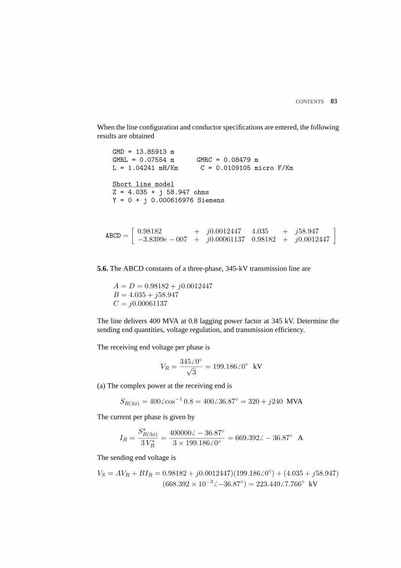
CONTENTS 83
When the line configuration and conductor specifications are entered, the followingresults are obtained
GMD = 13.85913 mGMRL = 0.07554 m GMRC = 0.08479 mL = 1.04241 mH/Km C = 0.0109105 micro F/Km
Short line modelZ = 4.035 + j 58.947 ohmsY = 0 + j 0.000616976 Siemens
ABCD =[
0.98182 + j0.0012447 4.035 + j58.947−3.8399e− 007 + j0.00061137 0.98182 + j0.0012447
]
5.6.The ABCD constants of a three-phase, 345-kV transmission line are
A = D = 0.98182 + j0.0012447B = 4.035 + j58.947C = j0.00061137
The line delivers 400 MVA at 0.8 lagging power factor at 345 kV. Determine thesending end quantities, voltage regulation, and transmission efficiency.
The receiving end voltage per phase is
VR =3456 0√
3= 199.1866 0 kV
(a) The complex power at the receiving end is
SR(3φ) = 4006 cos−1 0.8 = 4006 36.87 = 320 + j240 MVA
The current per phase is given by
IR =S∗R(3φ)
3V ∗R
=4000006 − 36.87
3× 199.1866 0= 669.3926 − 36.87 A
The sending end voltage is
VS = AVR + BIR = 0.98182 + j0.0012447)(199.1866 0) + (4.035 + j58.947)(668.392× 10⁻³ 6 −36.87) = 223.4496 7.766 kV
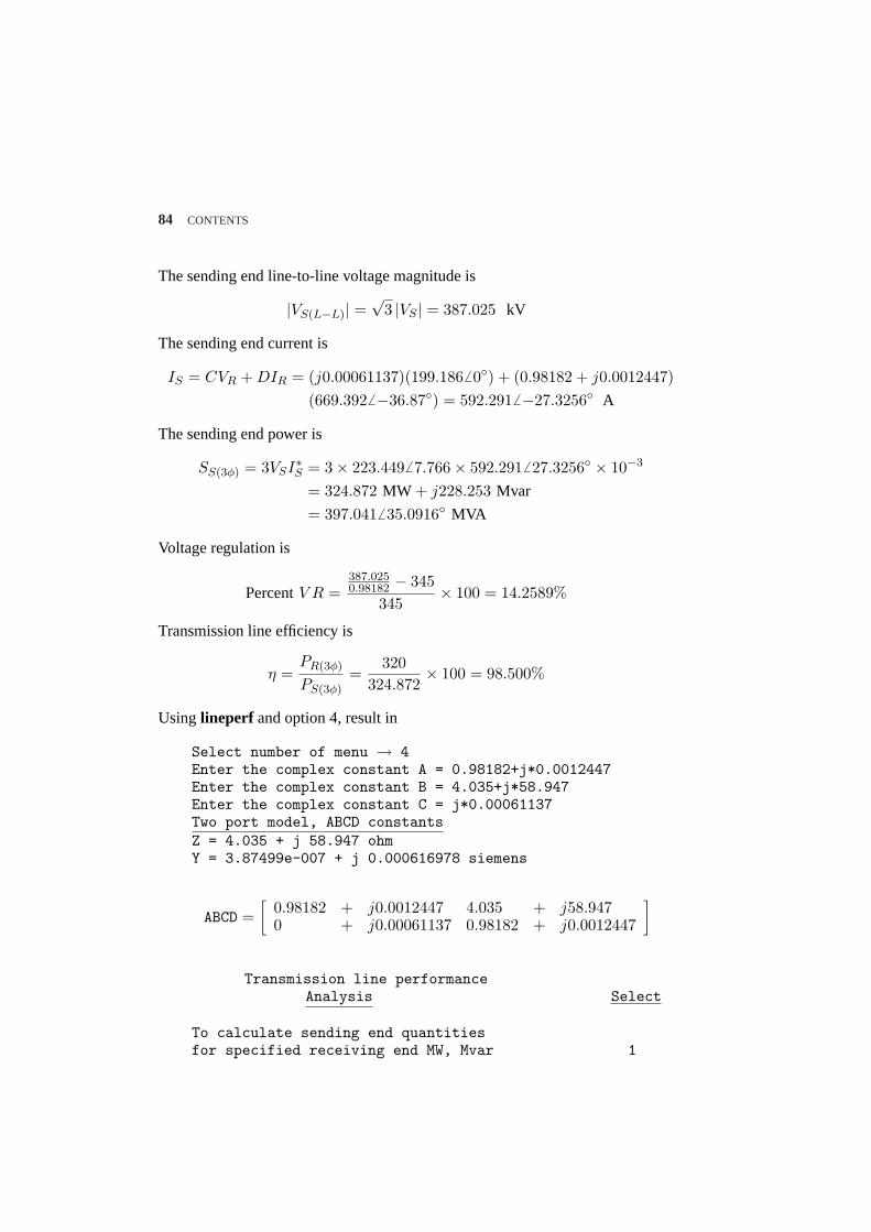
84 CONTENTS
The sending end line-to-line voltage magnitude is
|VS(L−L)| =√
3 |VS | = 387.025 kV
The sending end current is
IS = CVR + DIR = (j0.00061137)(199.1866 0) + (0.98182 + j0.0012447)(669.3926 −36.87) = 592.2916 −27.3256 A
The sending end power is
SS(3φ) = 3VSI∗S = 3× 223.4496 7.766× 592.2916 27.3256 × 10−3
= 324.872 MW + j228.253 Mvar
= 397.0416 35.0916 MVA
Voltage regulation is
PercentV R =387.0250.98182 − 345
345× 100 = 14.2589%
Transmission line efficiency is
η =PR(3φ)
PS(3φ)=
320324.872
× 100 = 98.500%
Using lineperf and option 4, result in
Select number of menu → 4Enter the complex constant A = 0.98182+j*0.0012447Enter the complex constant B = 4.035+j*58.947Enter the complex constant C = j*0.00061137Two port model, ABCD constantsZ = 4.035 + j 58.947 ohmY = 3.87499e-007 + j 0.000616978 siemens
ABCD =[
0.98182 + j0.0012447 4.035 + j58.9470 + j0.00061137 0.98182 + j0.0012447
]
Transmission line performanceAnalysis Select
To calculate sending end quantitiesfor specified receiving end MW, Mvar 1
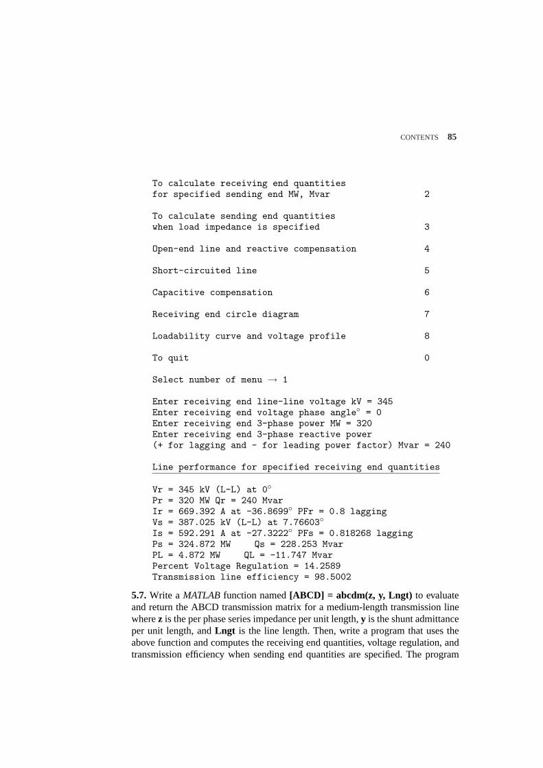
CONTENTS 85
To calculate receiving end quantitiesfor specified sending end MW, Mvar 2
To calculate sending end quantitieswhen load impedance is specified 3
Open-end line and reactive compensation 4
Short-circuited line 5
Capacitive compensation 6
Receiving end circle diagram 7
Loadability curve and voltage profile 8
To quit 0
Select number of menu → 1
Enter receiving end line-line voltage kV = 345Enter receiving end voltage phase angle = 0Enter receiving end 3-phase power MW = 320Enter receiving end 3-phase reactive power(+ for lagging and - for leading power factor) Mvar = 240
Line performance for specified receiving end quantities
Vr = 345 kV (L-L) at 0Pr = 320 MW Qr = 240 MvarIr = 669.392 A at -36.8699 PFr = 0.8 laggingVs = 387.025 kV (L-L) at 7.76603Is = 592.291 A at -27.3222 PFs = 0.818268 laggingPs = 324.872 MW Qs = 228.253 MvarPL = 4.872 MW QL = -11.747 MvarPercent Voltage Regulation = 14.2589Transmission line efficiency = 98.5002
5.7. Write a MATLAB function named[ABCD] = abcdm(z, y, Lngt) to evaluateand return the ABCD transmission matrix for a medium-length transmission linewherez is the per phase series impedance per unit length,y is the shunt admittanceper unit length, andLngt is the line length. Then, write a program that uses theabove function and computes the receiving end quantities, voltage regulation, andtransmission efficiency when sending end quantities are specified. The program

86 CONTENTS
should prompt the user to enter the following quantities:
The sending end line-to-line voltage magnitude in kVThe sending end voltage phase angle in degreesThe three-phase sending end real power in MWThe three-phase sending end reactive power in Mvar
Use your program to obtain the solution for the following case:
A three-phase transmission line has a per phase series impedance ofz = 0.03 +j0.4 Ω per Km and a per phase shunt admittance ofy = j4.0× 10−6 siemens perKm. The line is 125 Km long. Obtain the ABCD transmission matrix. Determinethe receiving end quantities, voltage regulation, and the transmission efficiencywhen the line is sending 407 MW, 7.833 Mvar at 350 kV.
The following function namedabcdm returns the line ABCD constants
function [ABCD] = abcdm(z, y, Lngt);Z = z*Lngt;Y = y*Lngt;A = 1 + Z*Y/2; B = Z;C = Y*(1 + Z*Y/4); D = A;ABCD = [A B; C D];
The following program saved asch5p7.mcomputes the receiving end quantitiesfrom the specified sending end quantities.
z=input(’Line series impedance per phase per unit length z=’);y=input(’Line shunt admittance per phase per unit length y=’);Lngt = input(’Transmission line length = ’);ABCD = abcdm(z, y,Lngt)VL_s=input(’Sending end line-to-line voltage magnitude in kV=’);AngV_s=input(’Sending end voltage phase angle in degree = ’);P_s =input(’Three-phase sending end real power in MW ’);Q_s =input(’Three-phase sending end reactive power in Mvar ’);S_s = P_s + j*Q_s; % MVAAngV_srd = AngV_s*pi/180; % RadianV_s = VL_s/sqrt(3)*(cos(AngV_srd) + j*sin(AngV_srd)); %kVI_s = conj(S_s)/(3*conj(V_s)); % kAIL_s= abs(I_s)*1000; AngI_srd = angle(I_s);AngI_s = AngI_srd*180/pi;VI_r = inv(ABCD)*[V_s; I_s];V_r = VI_r(1); VL_r = sqrt(3)*abs(V_r);AngV_rrd = angle(V_r); AngV_r = AngV_rrd*180/pi;
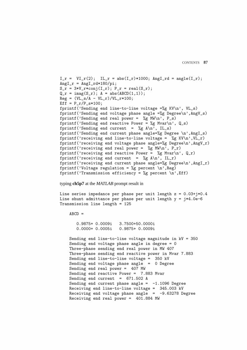
CONTENTS 87
I_r = VI_r(2); IL_r = abs(I_r)*1000; AngI_rd = angle(I_r);AngI_r = AngI_rd*180/pi;S_r = 3*V_r*conj(I_r); P_r = real(S_r);Q_r = imag(S_r); A = abs(ABCD(1,1));Reg = (VL_s/A - VL_r)/VL_r*100;Eff = P_r/P_s*100;fprintf(’Sending end line-to-line voltage =%g KV\n’, VL_s)fprintf(’Sending end voltage phase angle =%g Degree\n’,AngV_s)fprintf(’Sending end real power = %g MW\n’, P_s)fprintf(’Sending end reactive Power = %g Mvar\n’, Q_s)fprintf(’Sending end current = %g A\n’, IL_s)fprintf(’Sending end current phase angle=%g Degree \n’,AngI_s)fprintf(’receiving end line-to-line voltage = %g KV\n’,VL_r)fprintf(’receiving end voltage phase angle=%g Degree\n’,AngV_r)fprintf(’receiving end real power = %g MW\n’, P_r)fprintf(’receiving end reactive Power = %g Mvar\n’, Q_r)fprintf(’receiving end current = %g A\n’, IL_r)fprintf(’receiving end current phase angle=%g Degree\n’,AngI_r)fprintf(’Voltage regulation = %g percent \n’,Reg)fprintf(’Transmission efficiency = %g percent \n’,Eff)
typingch5p7at theMATLABprompt result in
Line series impedance per phase per unit length z = 0.03+j*0.4Line shunt admittance per phase per unit length y = j*4.0e-6Transmission line length = 125
ABCD =
0.9875+ 0.0009i 3.7500+50.0000i0.0000+ 0.0005i 0.9875+ 0.0009i
Sending end line-to-line voltage magnitude in kV = 350Sending end voltage phase angle in degree = 0Three-phase sending end real power in MW 407Three-phase sending end reactive power in Mvar 7.883Sending end line-to-line voltage = 350 kVSending end voltage phase angle = 0 DegreeSending end real power = 407 MWSending end reactive Power = 7.883 MvarSending end current = 671.502 ASending end current phase angle = -1.1096 DegreeReceiving end line-to-line voltage = 345.003 kVReceiving end voltage phase angle = -9.63278 DegreeReceiving end real power = 401.884 MW
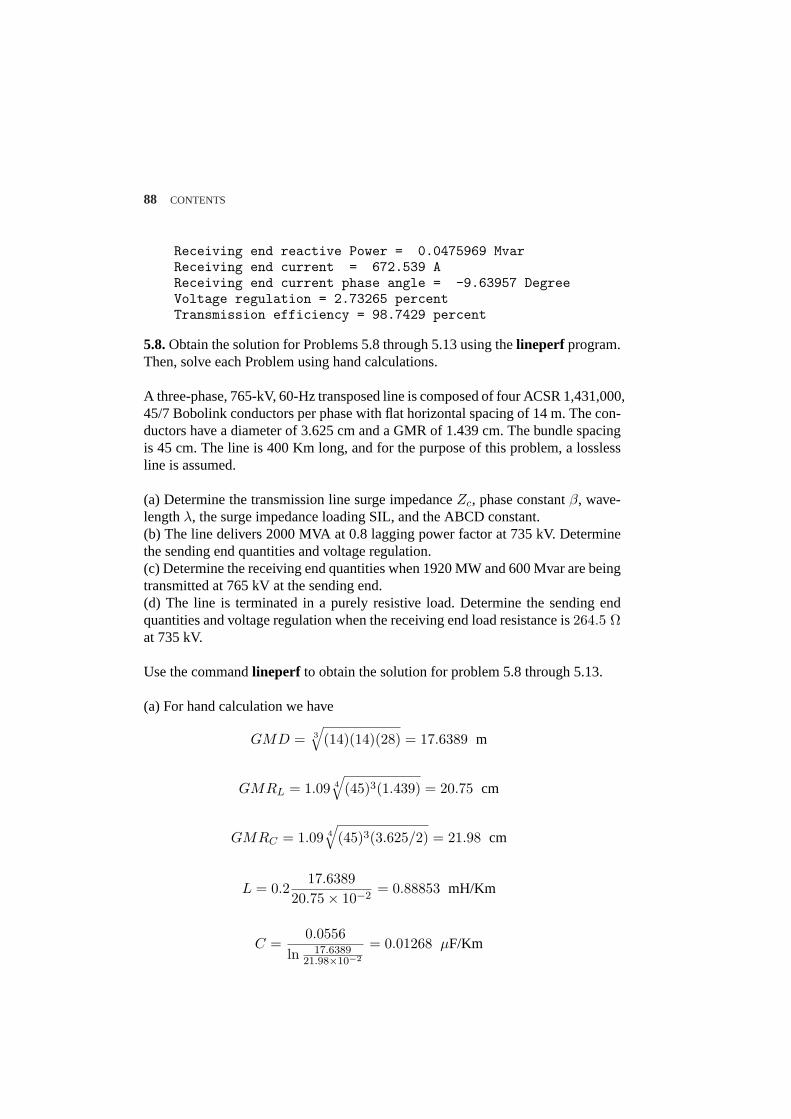
88 CONTENTS
Receiving end reactive Power = 0.0475969 MvarReceiving end current = 672.539 AReceiving end current phase angle = -9.63957 DegreeVoltage regulation = 2.73265 percentTransmission efficiency = 98.7429 percent
5.8.Obtain the solution for Problems 5.8 through 5.13 using thelineperf program.Then, solve each Problem using hand calculations.
A three-phase, 765-kV, 60-Hz transposed line is composed of four ACSR 1,431,000,45/7 Bobolink conductors per phase with flat horizontal spacing of 14 m. The con-ductors have a diameter of 3.625 cm and a GMR of 1.439 cm. The bundle spacingis 45 cm. The line is 400 Km long, and for the purpose of this problem, a losslessline is assumed.
(a) Determine the transmission line surge impedanceZc, phase constantβ, wave-lengthλ, the surge impedance loading SIL, and the ABCD constant.(b) The line delivers 2000 MVA at 0.8 lagging power factor at 735 kV. Determinethe sending end quantities and voltage regulation.(c) Determine the receiving end quantities when 1920 MW and 600 Mvar are beingtransmitted at 765 kV at the sending end.(d) The line is terminated in a purely resistive load. Determine the sending endquantities and voltage regulation when the receiving end load resistance is264.5 Ωat 735 kV.
Use the commandlineperf to obtain the solution for problem 5.8 through 5.13.
(a) For hand calculation we have
GMD = 3
√(14)(14)(28) = 17.6389 m
GMRL = 1.09 4
√(45)3(1.439) = 20.75 cm
GMRC = 1.09 4
√(45)3(3.625/2) = 21.98 cm
L = 0.217.6389
20.75× 10−2= 0.88853 mH/Km
C =0.0556
ln 17.638921.98×10−2
= 0.01268 µF/Km
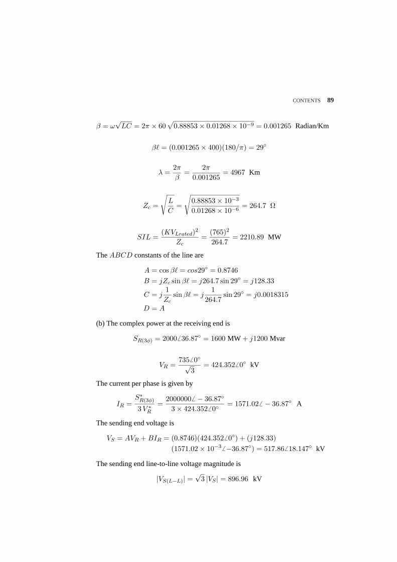
CONTENTS 89
β = ω√
LC = 2π × 60√
0.88853× 0.01268× 10−9 = 0.001265 Radian/Km
β` = (0.001265× 400)(180/π) = 29
λ =2π
β=
2π
0.001265= 4967 Km
Zc =
√L
C=
√0.88853× 10⁻³
0.01268× 10−6= 264.7 Ω
SIL =(KVLrated)2
Zc=
(765)2
264.7= 2210.89 MW
TheABCD constants of the line are
A = cos β` = cos29 = 0.8746B = jZc sinβ` = j264.7 sin 29 = j128.33
C = j1Zc
sinβ` = j1
264.7sin 29 = j0.0018315
D = A
(b) The complex power at the receiving end is
SR(3φ) = 20006 36.87 = 1600 MW + j1200 Mvar
VR =7356 0√
3= 424.3526 0 kV
The current per phase is given by
IR =S∗R(3φ)
3V ∗R
=20000006 − 36.87
3× 424.3526 0= 1571.02 6 − 36.87 A
The sending end voltage is
VS = AVR + BIR = (0.8746)(424.3526 0) + (j128.33)(1571.02× 10−3 6 −36.87) = 517.866 18.147 kV
The sending end line-to-line voltage magnitude is
|VS(L−L)| =√
3 |VS | = 896.96 kV
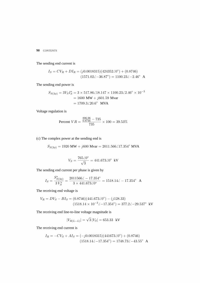
90 CONTENTS
The sending end current is
IS = CVR + DIR = (j0.0018315)(4243526 0) + (0.8746)(1571.026 −36.87) = 1100.23 6 −2.46 A
The sending end power is
SS(3φ) = 3VSI∗S = 3× 517.866 18.147× 1100.23 6 2.46 × 10−3
= 1600 MW + j601.59 Mvar
= 1709.36 20.6 MVA
Voltage regulation is
PercentV R =896.960.8746 − 735
735× 100 = 39.53%
(c) The complex power at the sending end is
SS(3φ) = 1920 MW + j600 Mvar = 2011.5666 17.354 MVA
VS =7656 0√
3= 441.6736 0 kV
The sending end current per phase is given by
IS =S∗S(3φ)
3V ∗S
=20115666 − 17.354
3× 441.6736 0= 1518.14 6 − 17.354 A
The receiving end voltage is
VR = DVS −BIS = (0.8746)(441.6736 0)− (j128.33)(1518.14× 10−3 6 −17.354) = 377.26 −29.537 kV
The receiving end line-to-line voltage magnitude is
|VR(L−L)| =√
3 |VS | = 653.33 kV
The receiving end current is
IR = −CVS + AIS = (−j0.0018315)(4416736 0) + (0.8746)(1518.146 −17.354) = 1748.73 6 −43.55 A
CONTENTS 91
The receiving end power is
SR(3φ) = 3VRI∗R = 3× 377.2 6 − 29.537 × 1748.736 43.55 × 10−3
= 1920 MW + j479.2 Mvar
= 1978.866 14.013 MVA
Voltage regulation is
PercentV R =765
0.8746 − 653.33653.33
× 100 = 33.88%
(d)
VR =7356 0√
3= 424.3526 0 kV
The receiving end current per phase is given by
IR =VR
ZL=
4243526 0
264.5= 1604.3576 0 A
The complex power at the receiving end is
SR(3φ) = 3VRIR∗ = 3(424.3526 0)(1604.3576 0)× 10−3 = 2042.44 MW
The sending end voltage is
VS = AVR + BIR = (0.8746)(424.3526 0) + (j128.33)= (1604.357× 10−3 6 0) = 424.42 6 29.02 kV
The sending end line-to-line voltage magnitude is
|VS(L−L)| =√
3 |VS | = 735.12 kV
The sending end current is
IS = CVR + DIR = (j0.0018315)(4243526 0) + (0.8746)(1604.3576 0) = 1604.04 6 28.98 A
The sending end power is
SS(3φ) = 3VSI∗S = 3× 424.426 29.02× 1604.04 6 − 28.98 × 10−3
= 2042.4 MW + j1.4 Mvar
= 2042.366 0.04 MVA
92 CONTENTS
Voltage regulation is
PercentV R =735.120.8746 − 735
735× 100 = 14.36%
5.9.The transmission line of Problem 5.8 is energized with 765 kV at the sendingend when the load at the receiving end is removed.
(a) Find the receiving end voltage.(b) Determine the reactance and the Mvar of a three-phase shunt reactor to beinstalled at the receiving end in order to limit the no-load receiving end voltage to735 kV.(a) The sending end voltage per phase is
VS =7656 0√
3= 441.6736 0 kV
When line is openIR = 0 and from (5.71) the no-load receiving end voltage isgiven by
VR(nl) =VS
cosβ`=
441.6730.8746
= 505 kV
The no-load receiving end line-to-line voltage is
VR(L−L)(nl) =√
3VR(nl) = 874.68 kV
(b) ForVRLL = 735 kV, the required inductor reactance given by (5.100) is
XLsh =sin(29)
765735 − cos(29)
(264.7) = 772.13 Ω
The three-phase shunt reactor rating is
Q3φ =(KVLrated)2
XLsh=
(735)2
772.13= 699.65 Mvar
5.10.The transmission line of Problem 5.8 is energized with 765 kV at the sendingend when a three-phase short-circuit occurs at the receiving end. Determine thereceiving end current and the sending end current.
For a solid short at the receiving end,VR = 0 and from (5.71) and (5.72) we have
Vs = jZc sinβ`IR
CONTENTS 93
or
IR =765000/
√3
j264.7 sin 29= 3441.76 − 90 A
IS = cosβ`IR = (cos 29)(3441.7 6 − 90) = 30106 − 90 A
5.11.Shunt capacitors are installed at the receiving end to improve the line per-formance of Problem 5.8. The line delivers 2000 MVA, 0.8 lagging power factor.Determine the total Mvar and the capacitance per phase of the Y-connected capac-itors to keep the receiving end voltage at 735 kV when the sending end voltage is765 kV.Hint: Use (5.93) and (5.94) to compute the power angleδ and the receivingend reactive power. Find the sending end quantities and voltage regulation for thecompensated line.
(a) The equivalent line reactance for a lossless line is given by
X ′ = Zc sinβ` = 264.7 sin(29) = 128.33 Ω
The receiving end power is
SR(3φ) = 20006 cos−1(0.8) = 1600 + j1200 MVA
For the above operating condition, the power angleδ is obtained from (5.93)
1600 =(765)(735)
128.33sin δ
which results inδ = 21.418. Using the approximate relation given by (5.94), thenet reactive power at the receiving end is
QR(3φ) =(765)(735)
128.33cos(21.418)− (735)2
128.33cos(29) = 397.05 Mvar
Thus, the required capacitor Mvar isSC = j397.05 − j1200 = −j802.95. Thecapacitive reactance is given by
XC =|VL|2S∗C
=(735)2
j802.95= −j672.8 Ω
or
C =106
2π(60)(672.8)= 3.9426 µF
94 CONTENTS
The net receiving end complex power is
SR(3φ) = 1600 + j397.05 = 1648.536 13.936 MVA
The receiving end current is
IR =1600− j397.05)103
3(424.3526 0)= 1294.946 −13.9368 A
We can check the sending end voltage
VS = AVR + BIR = (0.8746)(424.3526 0) + (j128.33)(1294.94× 10−3 6 − 13.9368) = 441.67 6 21.418 KV
or
|VS(L−L)| =√
3 |VS | = 765 kV
The sending end current is
IS = CVR + DIR = (j0.0018315)(4243526 0) + (0.8746)(1294.946 − 13.9368) = 1209.466 24.65 A
The sending end power is
SS(3φ) = 3VSI∗S = 3× 441.676 21.418× 1209.46 6 − 24.65 × 10−3
= 1600 MW − j90.35 Mvar
= 1602.556 − 3.23 MVA
Voltage regulation is
PercentV R =765
0.8746 − 735735
× 100 = 19.00%
5.12. Series capacitors are installed at the midpoint of the line of Problem 5.8,providing40 percent compensation. Determine the sending end quantities and thevoltage regulation when the line delivers 2000 MVA at 0.8 lagging power factor at735 kV.
For 40 percent compensation, the series capacitor reactance per phase is
Xser = 0.4×X ′ = 0.4(128.33) = 51.33 Ω
or
C =106
2π(60)(51.33)= 51.67 µF
CONTENTS 95
The new equivalentπ circuit parameters are given by
Z ′ = j(X ′ −Xser) = j(128.33− 51.33) = j77 Ω
Y ′ = = j2Zc
tan(β`/2) = j2
264.7tan(29/2) = j0.001954 siemens
The newB constant isB = j77 and the newA andC constants are given by
A = 1 +Z ′Y ′
2= 1 +
(j77)(j0.001954)2
= 0.92476
C = Y ′(
1 +Z ′Y ′
4
)= j0.001954
(1 +
(j77)(j0.001954)4
)= 0.0018805
The receiving end voltage per phase is
VR =735√
3= 424.352 kV
and the receiving end current is
IR =S∗R(3φ)
3V ∗R
=20006 −36.87
3× 424.356 0= 1.571026 −36.87 kA
Thus, the sending end voltage is
VS = AVR + BIR = 0.92476× 424.352 + j77× 1.571026 −36.87
= 474.9686 11.756 kV
and the line-to-line voltage magnitude is|VS(L−L)| =√
3VS = 822.67 kV. Thesending end current is
IS = CVR + DIR = (j0.0018805)(4243526 0) + (0.92476)(1571.026 − 36.87) = 1164.59 6 −3.628 A
The sending end power is
SS(3φ) = 3VSI∗S = 3× 474.9686 11.756× 1164.59 6 3.628 × 10−3
= 1600 MW + j440.2 Mvar
= 1659.4 6 15.38 MVA
Voltage regulation is
PercentV R =822.67/0.92476− 735
735× 100 = 21.035%
96 CONTENTS
5.13.Series capacitors are installed at the midpoint of the line of Problem 5.8, pro-viding 40 percent compensation. In addition, shunt capacitors are installed at thereceiving end. The line delivers 2000 MVA, 0.8 lagging power factor. Determinethe total Mvar and the capacitance per phase of the series and shunt capacitors tokeep the receiving end voltage at 735 kV when the sending end voltage is 765 kV.Find the sending end quantities and voltage regulation for the compensated line.
The receiving end power is
SR(3φ) = 20006 cos−1(0.8) = 1600 + j1200 MVA
With the series reactanceX ′ = 77 Ω, andcosβ` = A = 0.92476, the power angleδ is obtained from (5.93)
1600 =(765)(735)
77sin δ
which results inδ = 12.657. Using the approximate relation given by (5.94), thenet reactive power at the receiving end is
QR(3φ) =(765)(735)
77cos(12.657)− (735)2
770.92476 = 636.75 Mvar
Thus, the required shunt capacitor Mvar isSC = j636.75 − j1200 = −j563.25.The shunt capacitive reactance is given by
XC =|VL|2S∗C
=(735)2
j563.25= −j959.12 Ω
or
C =106
2π(60)(959.12)= 2.765 µF
The net receiving end complex power is
SR(3φ) = 1600 + j636.75 = 1722.056 21.7 MVA
The receiving end current is
IR =(1600− j636.75)103
3(424.3526 0)= 1352.696 −21.7 A
We can check the sending end voltage
VS = AVR + BIR = (0.92476)(424.3526 0) + (j77)(1352.69× 10−3 6 − 21.7) = 441.67 6 12.657 kV
CONTENTS 97
or
|VS(L−L)| =√
3 |VS | = 765 kV
The sending end current is
IS = CVR + DIR = (j0.0018805)(4243526 0) + (0.92476)(1352.696 − 21.7) = 1209.76 16.1 A
The sending end power is
SS(3φ) = 3VSI∗S = 3× 441.676 12.657× 1209.7 6 − 16.1 × 10−3
= 1600 MW − j96.3 Mvar
= 1602.96 − 3.44 MVA
Voltage regulation is
PercentV R =765
0.92476 − 735735
× 100 = 12.55%
5.14.The transmission line of Problem 5.8 has a per phase resistance of0.011 Ωper km. Using thelineperf program, perform the following analysis and present asummary of the calculation along with your conclusions and recommendations.
(a) Determine the sending end quantities for the specified receiving end quantitiesof 7356 0 kV, 1600 MW,1200 Mvar.(b) Determine the receiving end quantities for the specified sending end quantitiesof 7656 0 kV, 1920 MW,600 Mvar.(c) Determine the sending end quantities for a load impedance of282.38+ j0 Ω at735 kV.(d) Find the receiving end voltage when the line is terminated in an open circuitand is energized with 765 kV at the sending end. Also, determine the reactance andthe Mvar of a three-phase shunt reactor to be installed at the receiving end in orderto limit the no-load receiving end voltage to 765 kV. Obtain the voltage profile forthe uncompensated and the compensated line.(e) Find the receiving end and the sending end current when the line is terminatedin a three-phase short circuit.(f) For the line loading of part (a), determine the Mvar and the capacitance of theshunt capacitors to be installed at the receiving end to keep the receiving end volt-age at 735 kV when line is energized with 765 kV. Obtain the line performance ofthe compensated line.(g) Determine the line performance when the line is compensated by series capac-itor for 40 percent compensation with the load condition in part (a) at 735 kV.
98 CONTENTS
(h) The line has40 percent series capacitor compensation and supplies the loadin part (a). Determine the Mvar and the capacitance of the shunt capacitors to beinstalled at the receiving end to keep the receiving end voltage at 735 kV when lineis energized with 765 kV at the sending end.(i) Obtain the receiving end circle diagram.(j) Obtain the line voltage profile for a sending end voltage of 765 kV.(k) Obtain the line loadability curves when the sending end voltage is 765 kV, andthe receiving end voltage is 735 kV. The current-carrying capacity of the line is5000 A per phase.
Uselineperf to perform all the above analyses.
5.15.The ABCD constants of a lossless three-phase, 500-kV transmission line are
A = D = 0.86 + j0B = 0 + j130.2C = j0.002
(a) Obtain the sending end quantities and the voltage regulation when line delivers1000 MVA at 0.8 lagging power factor at 500 kV.
To improve the line performance, series capacitors are installed at both endsin each phase of the transmission line. As a result of this, the compensated ABCDconstants become
[A′ B′C ′ D′
]=
[1 −1
2jXc
0 1
] [A BC D
] [1 −1
2jXc
0 1
]
whereXc is the total reactance of the series capacitor. IfXc = 100 Ω(b) Determine the compensated ABCD constants.(c) Determine the sending end quantities and the voltage regulation when line de-livers 1000 MVA at 0.8 lagging power factor at 500 kV.
(a) The receiving end voltage per phase is
VR =5006 0√
3= 288.6756 0 kV
(a) The complex power at the receiving end is
SR(3φ) = 10006 cos−1 0.8 = 10006 36.87 = 800 + j600 MVA
The current per phase is given by
IR =S∗R(3φ)
3V ∗R
=10000006 − 36.87
3× 288.6756 0= 1154.76 − 36.87 A
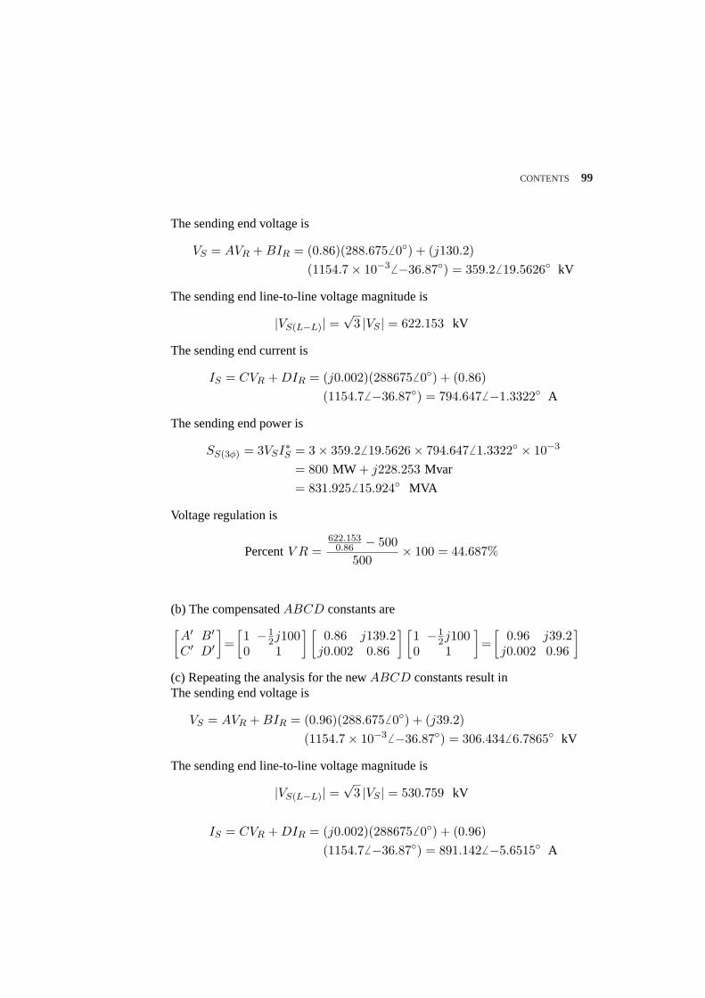
CONTENTS 99
The sending end voltage is
VS = AVR + BIR = (0.86)(288.6756 0) + (j130.2)(1154.7× 10−3 6 −36.87) = 359.26 19.5626 kV
The sending end line-to-line voltage magnitude is
|VS(L−L)| =√
3 |VS | = 622.153 kV
The sending end current is
IS = CVR + DIR = (j0.002)(2886756 0) + (0.86)(1154.76 −36.87) = 794.6476 −1.3322 A
The sending end power is
SS(3φ) = 3VSI∗S = 3× 359.2 6 19.5626× 794.6476 1.3322 × 10−3
= 800 MW + j228.253 Mvar
= 831.9256 15.924 MVA
Voltage regulation is
PercentV R =622.153
0.86 − 500500
× 100 = 44.687%
(b) The compensatedABCD constants are[A′ B′C ′ D′
]=
[1 −1
2j1000 1
] [0.86 j139.2
j0.002 0.86
] [1 −1
2j1000 1
]=
[0.96 j39.2
j0.002 0.96
]
(c) Repeating the analysis for the newABCD constants result inThe sending end voltage is
VS = AVR + BIR = (0.96)(288.6756 0) + (j39.2)(1154.7× 10−3 6 −36.87) = 306.4346 6.7865 kV
The sending end line-to-line voltage magnitude is
|VS(L−L)| =√
3 |VS | = 530.759 kV
IS = CVR + DIR = (j0.002)(2886756 0) + (0.96)(1154.76 −36.87) = 891.1426 −5.6515 A
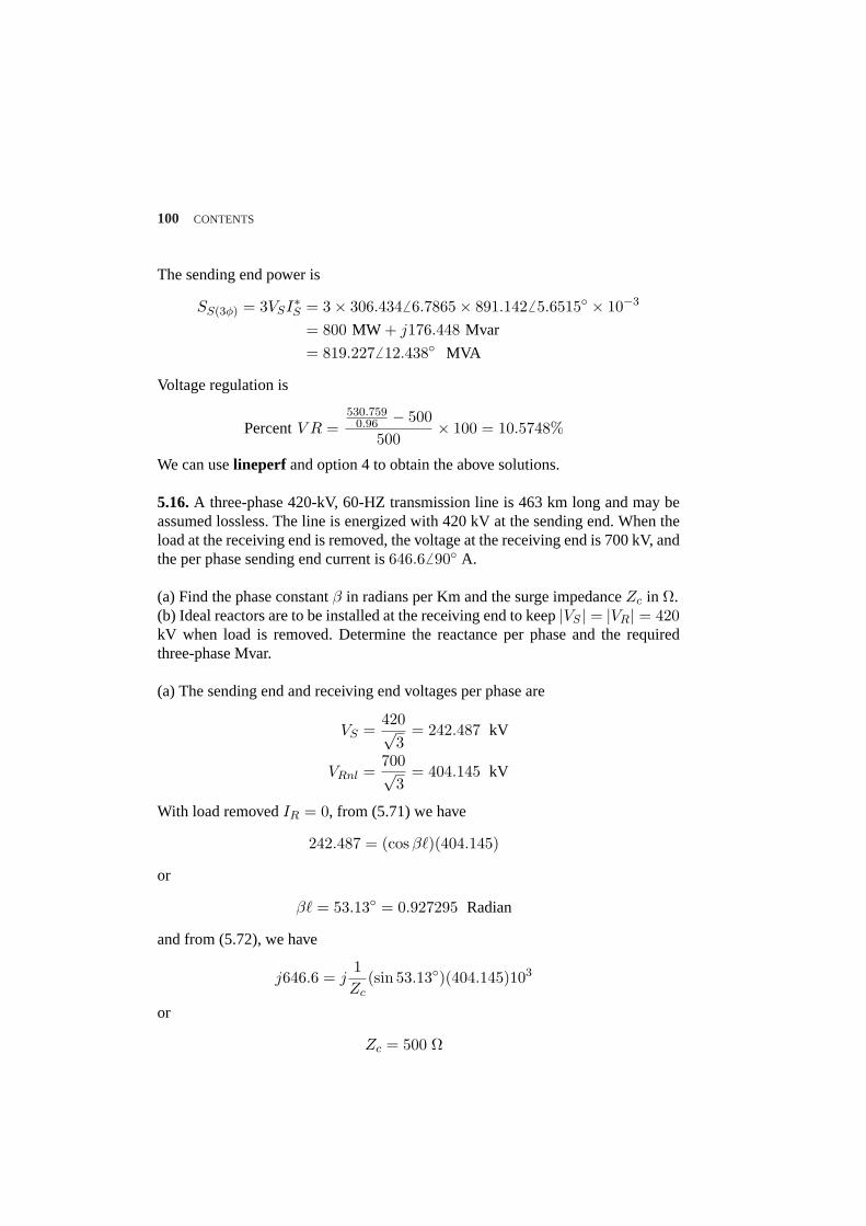
100 CONTENTS
The sending end power is
SS(3φ) = 3VSI∗S = 3× 306.4346 6.7865× 891.1426 5.6515 × 10−3
= 800 MW + j176.448 Mvar
= 819.2276 12.438 MVA
Voltage regulation is
PercentV R =530.759
0.96 − 500500
× 100 = 10.5748%
We can uselineperf and option 4 to obtain the above solutions.
5.16.A three-phase 420-kV, 60-HZ transmission line is 463 km long and may beassumed lossless. The line is energized with 420 kV at the sending end. When theload at the receiving end is removed, the voltage at the receiving end is 700 kV, andthe per phase sending end current is646.66 90 A.
(a) Find the phase constantβ in radians per Km and the surge impedanceZc in Ω.(b) Ideal reactors are to be installed at the receiving end to keep|VS | = |VR| = 420kV when load is removed. Determine the reactance per phase and the requiredthree-phase Mvar.
(a) The sending end and receiving end voltages per phase are
VS =420√
3= 242.487 kV
VRnl =700√
3= 404.145 kV
With load removedIR = 0, from (5.71) we have
242.487 = (cosβ`)(404.145)
or
β` = 53.13 = 0.927295 Radian
and from (5.72), we have
j646.6 = j1Zc
(sin 53.13)(404.145)103
or
Zc = 500 Ω
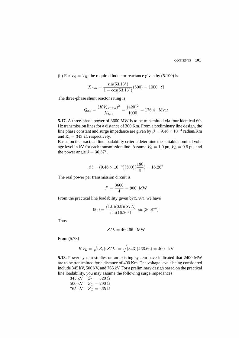
CONTENTS 101
(b) ForVS = VR, the required inductor reactance given by (5.100) is
XLsh =sin(53.13)
1− cos(53.13)(500) = 1000 Ω
The three-phase shunt reactor rating is
Q3φ =(KVLrated)2
XLsh=
(420)2
1000= 176.4 Mvar
5.17.A three-phase power of 3600 MW is to be transmitted via four identical 60-Hz transmission lines for a distance of 300 Km. From a preliminary line design, theline phase constant and surge impedance are given byβ = 9.46× 10⁻⁴ radian/KmandZc = 343 Ω, respectively.Based on the practical line loadability criteria determine the suitable nominal volt-age level in kV for each transmission line. AssumeVS = 1.0 pu,VR = 0.9 pu, andthe power angleδ = 36.87.
β` = (9.46× 10⁻⁴)(300)(180π
) = 16.26
The real power per transmission circuit is
P =3600
4= 900 MW
From the practical line loadability given by(5.97), we have
900 =(1.0)(0.9)(SIL)
sin(16.26)sin(36.87)
Thus
SIL = 466.66 MW
From (5.78)
KVL =√
(Zc)(SIL) =√
(343)(466.66) = 400 kV
5.18.Power system studies on an existing system have indicated that 2400 MWare to be transmitted for a distance of 400 Km. The voltage levels being consideredinclude 345 kV, 500 kV, and 765 kV. For a preliminary design based on the practicalline loadability, you may assume the following surge impedances
345 kV ZC = 320 Ω500 kV ZC = 290 Ω765 kV ZC = 265 Ω
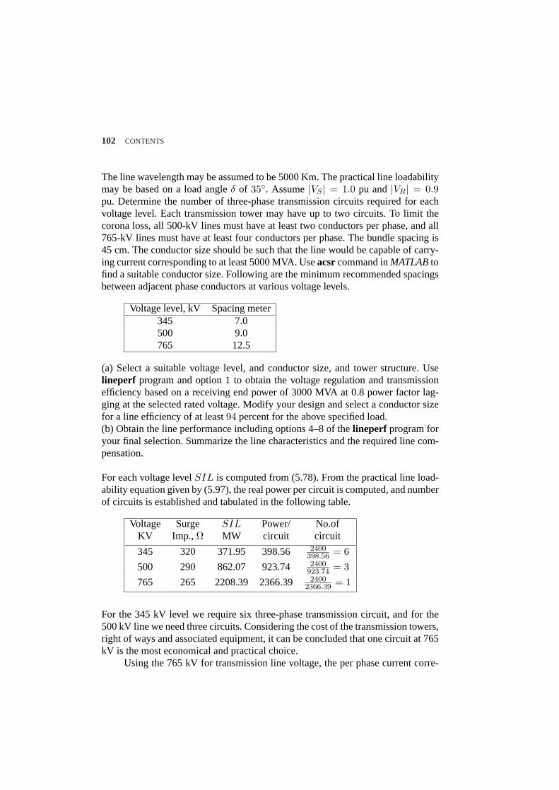
102 CONTENTS
The line wavelength may be assumed to be 5000 Km. The practical line loadabilitymay be based on a load angleδ of 35. Assume|VS | = 1.0 pu and|VR| = 0.9pu. Determine the number of three-phase transmission circuits required for eachvoltage level. Each transmission tower may have up to two circuits. To limit thecorona loss, all 500-kV lines must have at least two conductors per phase, and all765-kV lines must have at least four conductors per phase. The bundle spacing is45 cm. The conductor size should be such that the line would be capable of carry-ing current corresponding to at least 5000 MVA. Useacsrcommand inMATLABtofind a suitable conductor size. Following are the minimum recommended spacingsbetween adjacent phase conductors at various voltage levels.
Voltage level, kV Spacing meter345 7.0500 9.0765 12.5
(a) Select a suitable voltage level, and conductor size, and tower structure. Uselineperf program and option 1 to obtain the voltage regulation and transmissionefficiency based on a receiving end power of 3000 MVA at 0.8 power factor lag-ging at the selected rated voltage. Modify your design and select a conductor sizefor a line efficiency of at least94 percent for the above specified load.(b) Obtain the line performance including options 4–8 of thelineperf program foryour final selection. Summarize the line characteristics and the required line com-pensation.
For each voltage levelSIL is computed from (5.78). From the practical line load-ability equation given by (5.97), the real power per circuit is computed, and numberof circuits is established and tabulated in the following table.
Voltage Surge SIL Power/ No.ofKV Imp., Ω MW circuit circuit
345 320 371.95 398.56 2400398.56 = 6
500 290 862.07 923.74 2400923.74 = 3
765 265 2208.39 2366.39 24002366.39 = 1
For the 345 kV level we require six three-phase transmission circuit, and for the500 kV line we need three circuits. Considering the cost of the transmission towers,right of ways and associated equipment, it can be concluded that one circuit at 765kV is the most economical and practical choice.
Using the 765 kV for transmission line voltage, the per phase current corre-
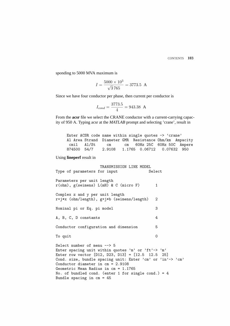
CONTENTS 103
sponding to 5000 MVA maximum is
I =5000× 103
√3 765
= 3773.5 A
Since we have four conductor per phase, then current per conductor is
Icond =3773.5
4= 943.38 A
From theacsr file we select the CRANE conductor with a current-carrying capac-ity of 950 A. Typing acsr at theMATLABprompt and selecting ’crane’, result in
Enter ACSR code name within single quotes -> ’crane’Al Area Strand Diameter GMR Resistance Ohm/km Ampacitycmil Al/St cm cm 60Hz 25C 60Hz 50C Ampere874500 54/7 2.9108 1.1765 0.06712 0.07632 950
Using lineperf result in
TRANSMISSION LINE MODELType of parameters for input Select
Parameters per unit lengthr(ohm), g(seimens) L(mH) & C (micro F) 1
Complex z and y per unit lengthr+j*x (ohm/length), g+j*b (seimens/length) 2
Nominal pi or Eq. pi model 3
A, B, C, D constants 4
Conductor configuration and dimension 5
To quit 0
Select number of menu --> 5Enter spacing unit within quotes ’m’ or ’ft’-> ’m’Enter row vector [D12, D23, D13] = [12.5 12.5 25]Cond. size, bundle spacing unit: Enter ’cm’ or ’in’-> ’cm’Conductor diameter in cm = 2.9108Geometric Mean Radius in cm = 1.1765No. of bundled cond. (enter 1 for single cond.) = 4Bundle spacing in cm = 45
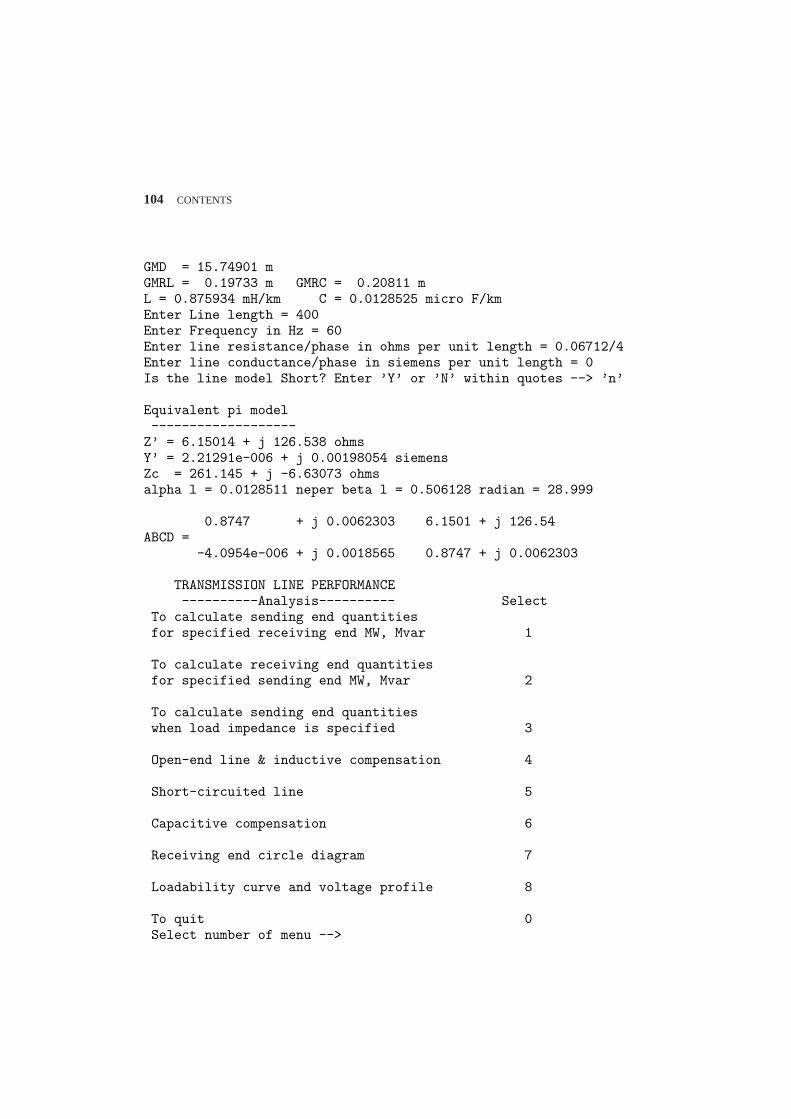
104 CONTENTS
GMD = 15.74901 mGMRL = 0.19733 m GMRC = 0.20811 mL = 0.875934 mH/km C = 0.0128525 micro F/kmEnter Line length = 400Enter Frequency in Hz = 60Enter line resistance/phase in ohms per unit length = 0.06712/4Enter line conductance/phase in siemens per unit length = 0Is the line model Short? Enter ’Y’ or ’N’ within quotes --> ’n’
Equivalent pi model-------------------
Z’ = 6.15014 + j 126.538 ohmsY’ = 2.21291e-006 + j 0.00198054 siemensZc = 261.145 + j -6.63073 ohmsalpha l = 0.0128511 neper beta l = 0.506128 radian = 28.999
0.8747 + j 0.0062303 6.1501 + j 126.54ABCD =
-4.0954e-006 + j 0.0018565 0.8747 + j 0.0062303
TRANSMISSION LINE PERFORMANCE----------Analysis---------- Select
To calculate sending end quantitiesfor specified receiving end MW, Mvar 1
To calculate receiving end quantitiesfor specified sending end MW, Mvar 2
To calculate sending end quantitieswhen load impedance is specified 3
Open-end line & inductive compensation 4
Short-circuited line 5
Capacitive compensation 6
Receiving end circle diagram 7
Loadability curve and voltage profile 8
To quit 0Select number of menu -->
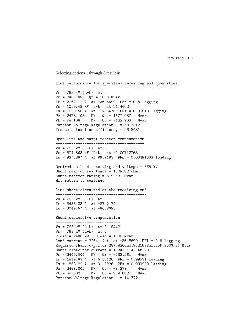
CONTENTS 105
Selecting options 1 through 8 result in
Line performance for specified receiving end quantities-------------------------------------------------------Vr = 765 kV (L-L) at 0Pr = 2400 MW Qr = 1800 MvarIr = 2264.12 A at -36.8699 PFr = 0.8 laggingVs = 1059.49 kV (L-L) at 21.4402Is = 1630.56 A at -12.6476 PFs = 0.82818 laggingPs = 2478.108 MW Qs = 1677.037 MvarPL = 78.108 MW QL = -122.963 MvarPercent Voltage Regulation = 58.3312Transmission line efficiency = 96.8481
Open line and shunt reactor compensation----------------------------------------Vs = 765 kV (L-L) at 0Vr = 874.563 kV (L-L) at -0.00712268Is = 937.387 A at 89.7183 PFs = 0.00491663 leading
Desired no load receiving end voltage = 765 kVShunt reactor reactance = 1009.82 ohmShunt reactor rating = 579.531 MvarHit return to continue
Line short-circuited at the receiving end-----------------------------------------Vs = 765 kV (L-L) at 0Ir = 3486.33 A at -87.2174Is = 3049.57 A at -86.8093
Shunt capacitive compensation-----------------------------Vs = 765 kV (L-L) at 31.8442Vr = 765 kV (L-L) at 0Pload = 2400 MW Qload = 1800 MvarLoad current = 2264.12 A at -36.8699 PFl = 0.8 laggingRequired shunt capcitor:287.826ohm,9.21593microF,2033.26 MvarShunt capacitor current = 1534.51 A at 90Pr = 2400.000 MW Qr = -233.261 MvarIr = 1819.83 A at 5.55126 PFr = 0.99531 leadingIs = 1863.22 A at 31.9226 PFs = 0.999999 leadingPs = 2468.802 MW Qs = -3.378 MvarPL = 68.802 MW QL = 229.882 MvarPercent Voltage Regulation = 14.322
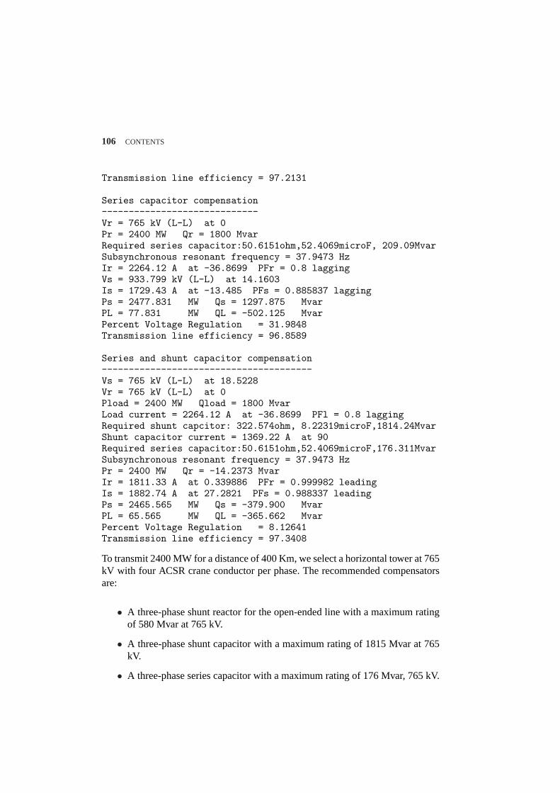
106 CONTENTS
Transmission line efficiency = 97.2131
Series capacitor compensation-----------------------------Vr = 765 kV (L-L) at 0Pr = 2400 MW Qr = 1800 MvarRequired series capacitor:50.6151ohm,52.4069microF, 209.09MvarSubsynchronous resonant frequency = 37.9473 HzIr = 2264.12 A at -36.8699 PFr = 0.8 laggingVs = 933.799 kV (L-L) at 14.1603Is = 1729.43 A at -13.485 PFs = 0.885837 laggingPs = 2477.831 MW Qs = 1297.875 MvarPL = 77.831 MW QL = -502.125 MvarPercent Voltage Regulation = 31.9848Transmission line efficiency = 96.8589
Series and shunt capacitor compensation---------------------------------------Vs = 765 kV (L-L) at 18.5228Vr = 765 kV (L-L) at 0Pload = 2400 MW Qload = 1800 MvarLoad current = 2264.12 A at -36.8699 PFl = 0.8 laggingRequired shunt capcitor: 322.574ohm, 8.22319microF,1814.24MvarShunt capacitor current = 1369.22 A at 90Required series capacitor:50.6151ohm,52.4069microF,176.311MvarSubsynchronous resonant frequency = 37.9473 HzPr = 2400 MW Qr = -14.2373 MvarIr = 1811.33 A at 0.339886 PFr = 0.999982 leadingIs = 1882.74 A at 27.2821 PFs = 0.988337 leadingPs = 2465.565 MW Qs = -379.900 MvarPL = 65.565 MW QL = -365.662 MvarPercent Voltage Regulation = 8.12641Transmission line efficiency = 97.3408
To transmit 2400 MW for a distance of 400 Km, we select a horizontal tower at 765kV with four ACSR crane conductor per phase. The recommended compensatorsare:
• A three-phase shunt reactor for the open-ended line with a maximum ratingof 580 Mvar at 765 kV.
• A three-phase shunt capacitor with a maximum rating of 1815 Mvar at 765kV.
• A three-phase series capacitor with a maximum rating of 176 Mvar, 765 kV.
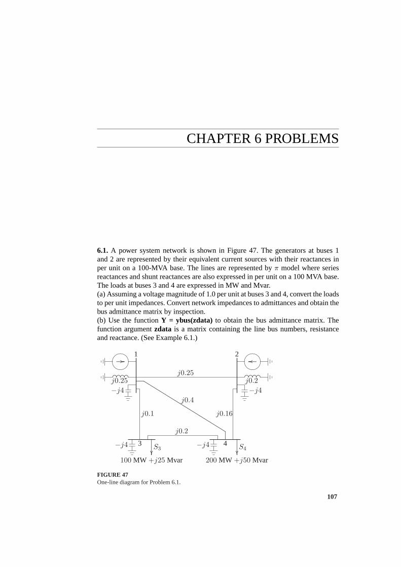
CHAPTER 6 PROBLEMS
6.1. A power system network is shown in Figure 47. The generators at buses 1and 2 are represented by their equivalent current sources with their reactances inper unit on a 100-MVA base. The lines are represented byπ model where seriesreactances and shunt reactances are also expressed in per unit on a 100 MVA base.The loads at buses 3 and 4 are expressed in MW and Mvar.(a) Assuming a voltage magnitude of 1.0 per unit at buses 3 and 4, convert the loadsto per unit impedances. Convert network impedances to admittances and obtain thebus admittance matrix by inspection.(b) Use the functionY = ybus(zdata) to obtain the bus admittance matrix. Thefunction argumentzdata is a matrix containing the line bus numbers, resistanceand reactance. (See Example 6.1.)
¹¸
º·
¹¸
º·
...............................................................................................................................................................................................................................................................................................................................................................................................................................
............................................. ................ .............................................................
............................................................................................ ............................................................................................
..................................................................
........
........
........
..................................................................
........
........
........
j0.25j0.25
j0.2−j4
−j4
−j4
j0.1 j0.16
j0.4
j0.2
−j4S3 S4
100 MW +j25 Mvar 200 MW +j50 Mvar
1 2
3 4
FIGURE 47One-line diagram for Problem 6.1.
107
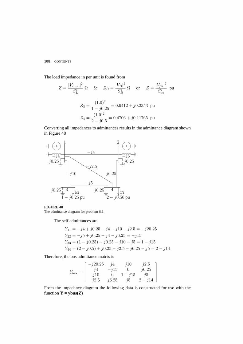
108 CONTENTS
The load impedance in per unit is found from
Z =|VL−L|2
S∗LΩ & ZB =
|VB|2S∗B
Ω or Z =|Vpu|2S∗pu
pu
Z3 =(1.0)2
1− j0.25= 0.9412 + j0.2353 pu
Z4 =(1.0)2
2− j0.5= 0.4706 + j0.11765 pu
Converting all impedances to admittances results in the admittance diagram shownin Figure 48
µ´¶³
µ´¶³
.............................................................................................................................................................................................................................................................................................................................................................................
.......................................... ................ ..........................................................
................................................................................ ................................................................................
...........................................................
........
........
........
...........................................................
........
........
........
−j4−j4
−j5j0.25
j0.25
j0.25
−j10 −j6.25
−j2.5
−j5
j0.25y3 y4
1− j0.25 pu 2− j0.50 pu
1 2
3 4
FIGURE 48The admittance diagram for problem 6.1.
The self admittances are
Y11 = −j4 + j0.25− j4− j10− j2.5 = −j20.25Y22 = −j5 + j0.25− j4− j6.25 = −j15Y33 = (1− j0.25) + j0.25− j10− j5 = 1− j15Y44 = (2− j0.5) + j0.25− j2.5− j6.25− j5 = 2− j14
Therefore, the bus admittance matrix is
Ybus =
−j20.25 j4 j10 j2.5j4 −j15 0 j6.25j10 0 1− j15 j5j2.5 j6.25 j5 2− j14
From the impedance diagram the following data is constructed for use with thefunctionY = ybus(Z)
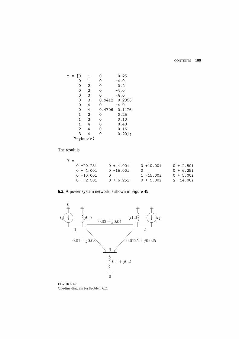
CONTENTS 109
z = [0 1 0 0.250 1 0 -4.00 2 0 0.20 2 0 -4.00 3 0 -4.00 3 0.9412 0.23530 4 0 -4.00 4 0.4706 0.11761 2 0 0.251 3 0 0.101 4 0 0.402 4 0 0.163 4 0 0.20];
Y=ybus(z)
The result is
Y =0 -20.25i 0 + 4.00i 0 +10.00i 0 + 2.50i0 + 4.00i 0 -15.00i 0 0 + 6.25i0 +10.00i 0 1 -15.00i 0 + 5.00i0 + 2.50i 0 + 6.25i 0 + 5.00i 2 -14.00i
6.2.A power system network is shown in Figure 49.
.........................................................
......................
......................
......................
......................
......................
......................
......................
..................................................................................................................................................................................................................................................................................................................................................................................................................................................................................................................................................................
........
........
........
...........................................................................
.......................
........
........
........
....
¹¸
º·
........
........
........
.....
........
........
........
.....
........
........
........
...........................................................................
.......................
........
........
........
....
¹¸
º·
........
........
........
.....
........
........
........
.....
.....................................
........
........
.....................................................................
........................................................................................................................................................................................................
1 2
3
0
0
I1 I2j0.5 j1.00.02 + j0.04
0.0125 + j0.0250.01 + j0.03
0.4 + j0.2
FIGURE 49One-line diagram for Problem 6.2.
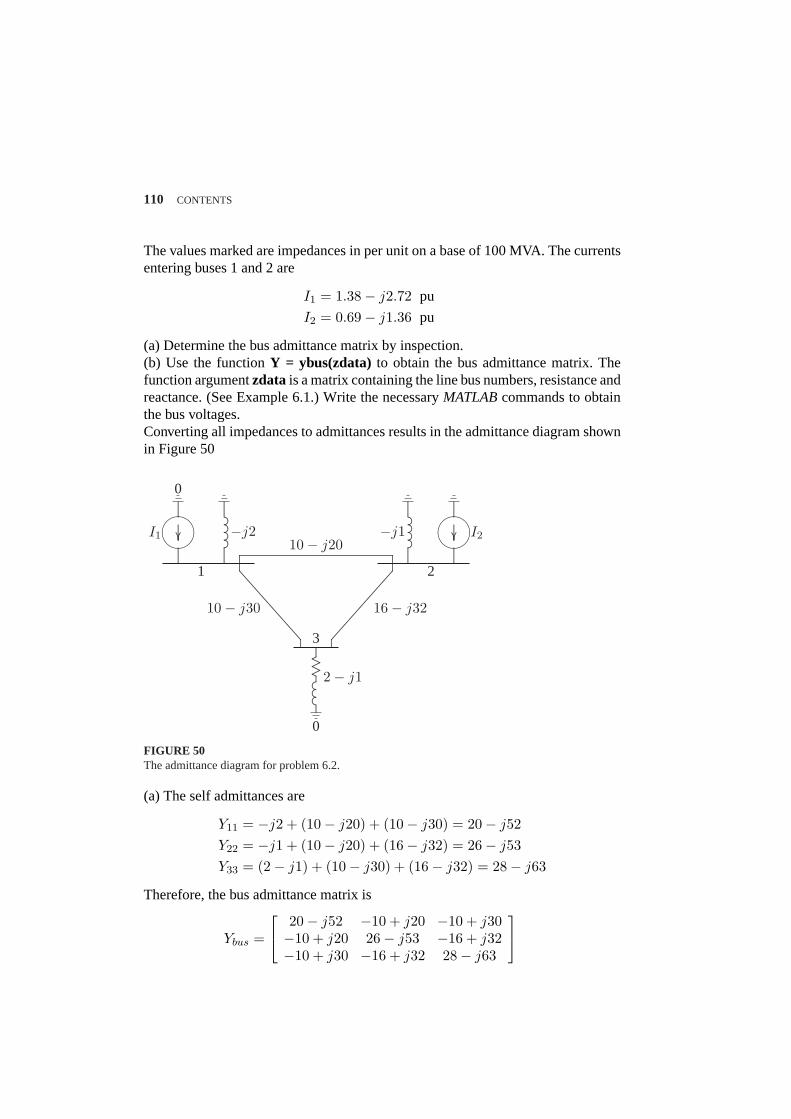
110 CONTENTS
The values marked are impedances in per unit on a base of 100 MVA. The currentsentering buses 1 and 2 are
I1 = 1.38− j2.72 pu
I2 = 0.69− j1.36 pu
(a) Determine the bus admittance matrix by inspection.(b) Use the functionY = ybus(zdata) to obtain the bus admittance matrix. Thefunction argumentzdata is a matrix containing the line bus numbers, resistance andreactance. (See Example 6.1.) Write the necessaryMATLABcommands to obtainthe bus voltages.Converting all impedances to admittances results in the admittance diagram shownin Figure 50
.........................................................
......................
......................
......................
......................
......................
......................
......................
..................................................................................................................................................................................................................................................................................................................................................................................................................................................................................................................................................................
........
........
........
...........................................................................
.......................
........
........
........
....
¹¸
º·
........
........
........
.....
........
........
........
.....
........
........
........
...........................................................................
.......................
........
........
........
....
¹¸
º·
........
........
........
.....
........
........
........
.....
.....................................
........
........
.....................................................................
........................................................................................................................................................................................................
1 2
3
0
0
I1 I2−j2 −j110− j20
16− j3210− j30
2− j1
FIGURE 50The admittance diagram for problem 6.2.
(a) The self admittances are
Y11 = −j2 + (10− j20) + (10− j30) = 20− j52Y22 = −j1 + (10− j20) + (16− j32) = 26− j53Y33 = (2− j1) + (10− j30) + (16− j32) = 28− j63
Therefore, the bus admittance matrix is
Ybus =
20− j52 −10 + j20 −10 + j30−10 + j20 26− j53 −16 + j32−10 + j30 −16 + j32 28− j63
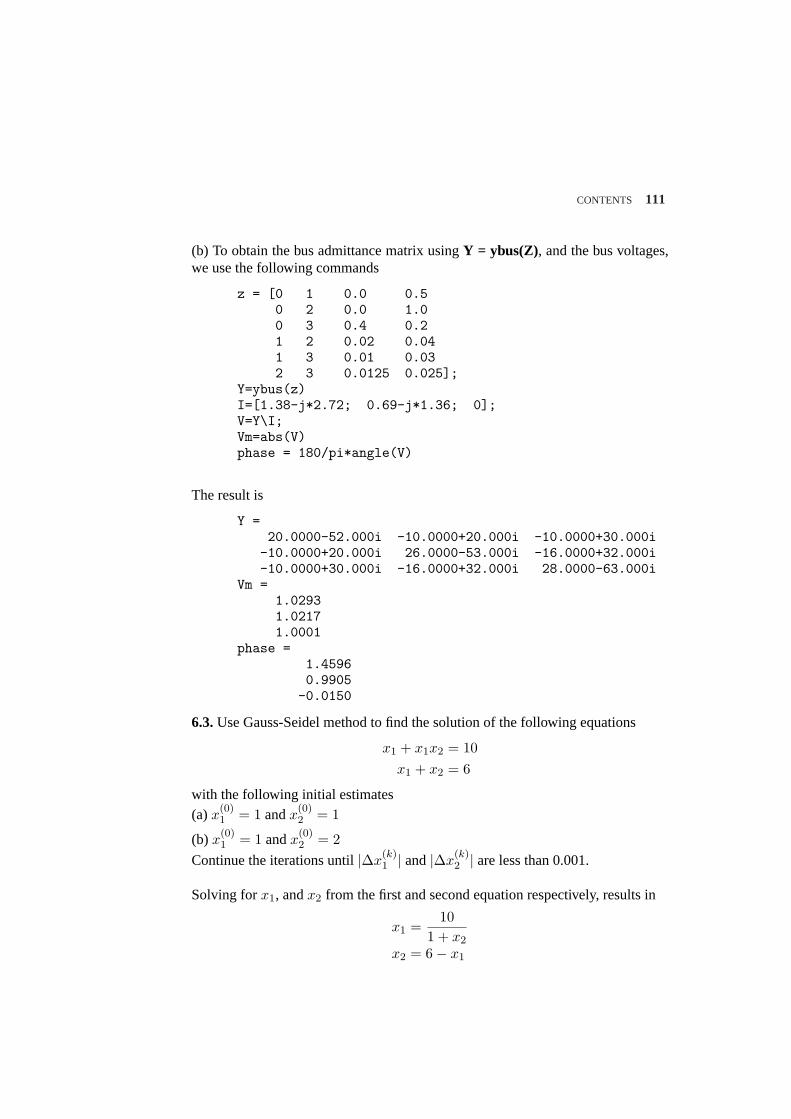
CONTENTS 111
(b) To obtain the bus admittance matrix usingY = ybus(Z), and the bus voltages,we use the following commands
z = [0 1 0.0 0.50 2 0.0 1.00 3 0.4 0.21 2 0.02 0.041 3 0.01 0.032 3 0.0125 0.025];
Y=ybus(z)I=[1.38-j*2.72; 0.69-j*1.36; 0];V=Y\I;Vm=abs(V)phase = 180/pi*angle(V)
The result is
Y =20.0000-52.000i -10.0000+20.000i -10.0000+30.000i
-10.0000+20.000i 26.0000-53.000i -16.0000+32.000i-10.0000+30.000i -16.0000+32.000i 28.0000-63.000i
Vm =1.02931.02171.0001
phase =1.45960.9905-0.0150
6.3.Use Gauss-Seidel method to find the solution of the following equations
x1 + x1x2 = 10x1 + x2 = 6
with the following initial estimates(a)x(0)
1 = 1 andx(0)2 = 1
(b) x(0)1 = 1 andx
(0)2 = 2
Continue the iterations until|∆x(k)1 | and|∆x
(k)2 | are less than 0.001.
Solving forx1, andx2 from the first and second equation respectively, results in
x1 =10
1 + x2
x2 = 6− x1
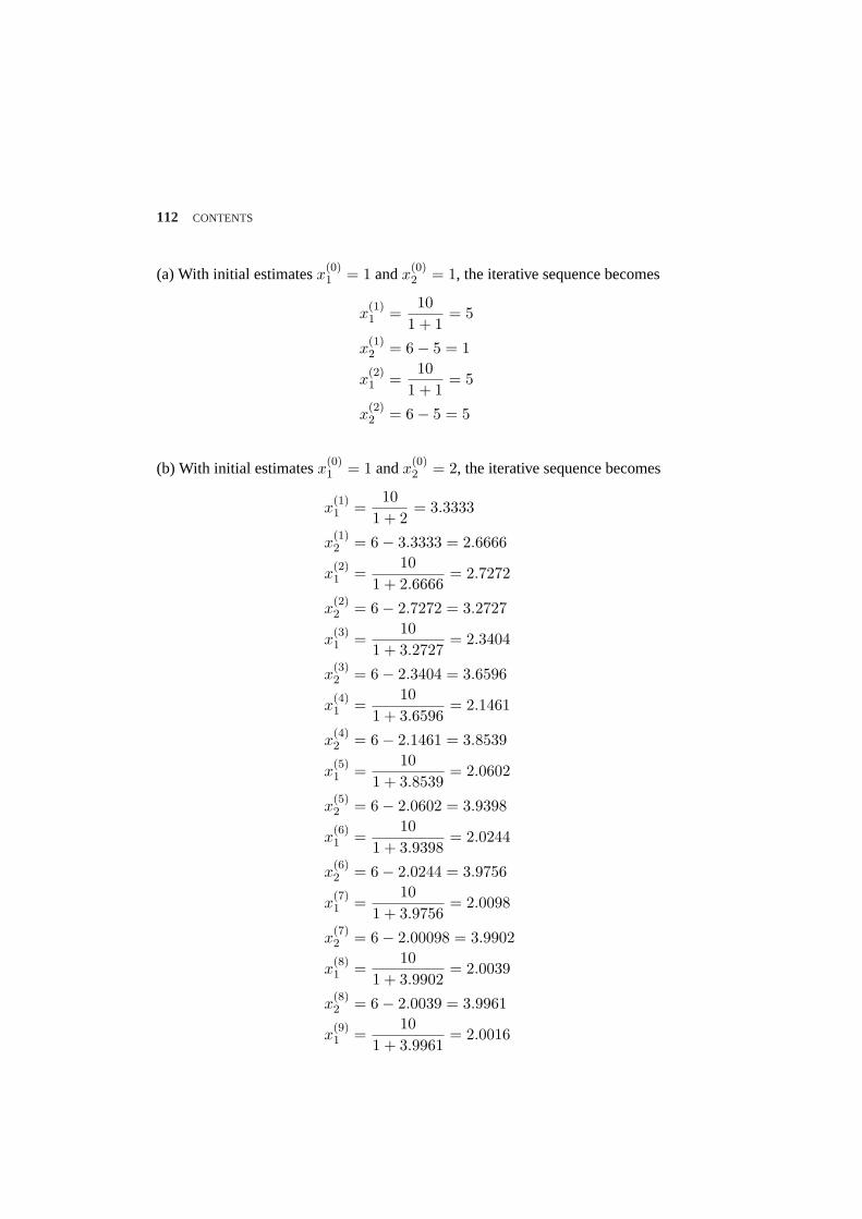
112 CONTENTS
(a) With initial estimatesx(0)1 = 1 andx
(0)2 = 1, the iterative sequence becomes
x(1)1 =
101 + 1
= 5
x(1)2 = 6− 5 = 1
x(2)1 =
101 + 1
= 5
x(2)2 = 6− 5 = 5
(b) With initial estimatesx(0)1 = 1 andx
(0)2 = 2, the iterative sequence becomes
x(1)1 =
101 + 2
= 3.3333
x(1)2 = 6− 3.3333 = 2.6666
x(2)1 =
101 + 2.6666
= 2.7272
x(2)2 = 6− 2.7272 = 3.2727
x(3)1 =
101 + 3.2727
= 2.3404
x(3)2 = 6− 2.3404 = 3.6596
x(4)1 =
101 + 3.6596
= 2.1461
x(4)2 = 6− 2.1461 = 3.8539
x(5)1 =
101 + 3.8539
= 2.0602
x(5)2 = 6− 2.0602 = 3.9398
x(6)1 =
101 + 3.9398
= 2.0244
x(6)2 = 6− 2.0244 = 3.9756
x(7)1 =
101 + 3.9756
= 2.0098
x(7)2 = 6− 2.00098 = 3.9902
x(8)1 =
101 + 3.9902
= 2.0039
x(8)2 = 6− 2.0039 = 3.9961
x(9)1 =
101 + 3.9961
= 2.0016
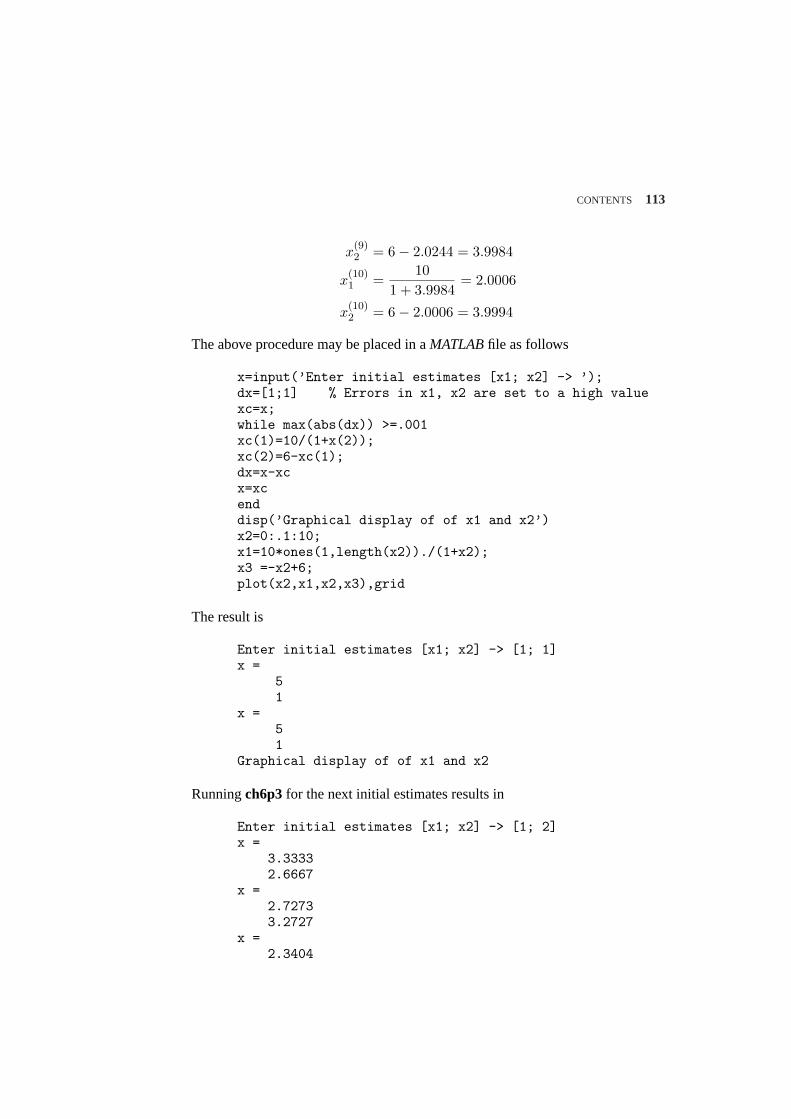
CONTENTS 113
x(9)2 = 6− 2.0244 = 3.9984
x(10)1 =
101 + 3.9984
= 2.0006
x(10)2 = 6− 2.0006 = 3.9994
The above procedure may be placed in aMATLABfile as follows
x=input(’Enter initial estimates [x1; x2] -> ’);dx=[1;1] % Errors in x1, x2 are set to a high valuexc=x;while max(abs(dx)) >=.001xc(1)=10/(1+x(2));xc(2)=6-xc(1);dx=x-xcx=xcenddisp(’Graphical display of of x1 and x2’)x2=0:.1:10;x1=10*ones(1,length(x2))./(1+x2);x3 =-x2+6;plot(x2,x1,x2,x3),grid
The result is
Enter initial estimates [x1; x2] -> [1; 1]x =
51
x =51
Graphical display of of x1 and x2
Runningch6p3for the next initial estimates results in
Enter initial estimates [x1; x2] -> [1; 2]x =
3.33332.6667
x =2.72733.2727
x =2.3404
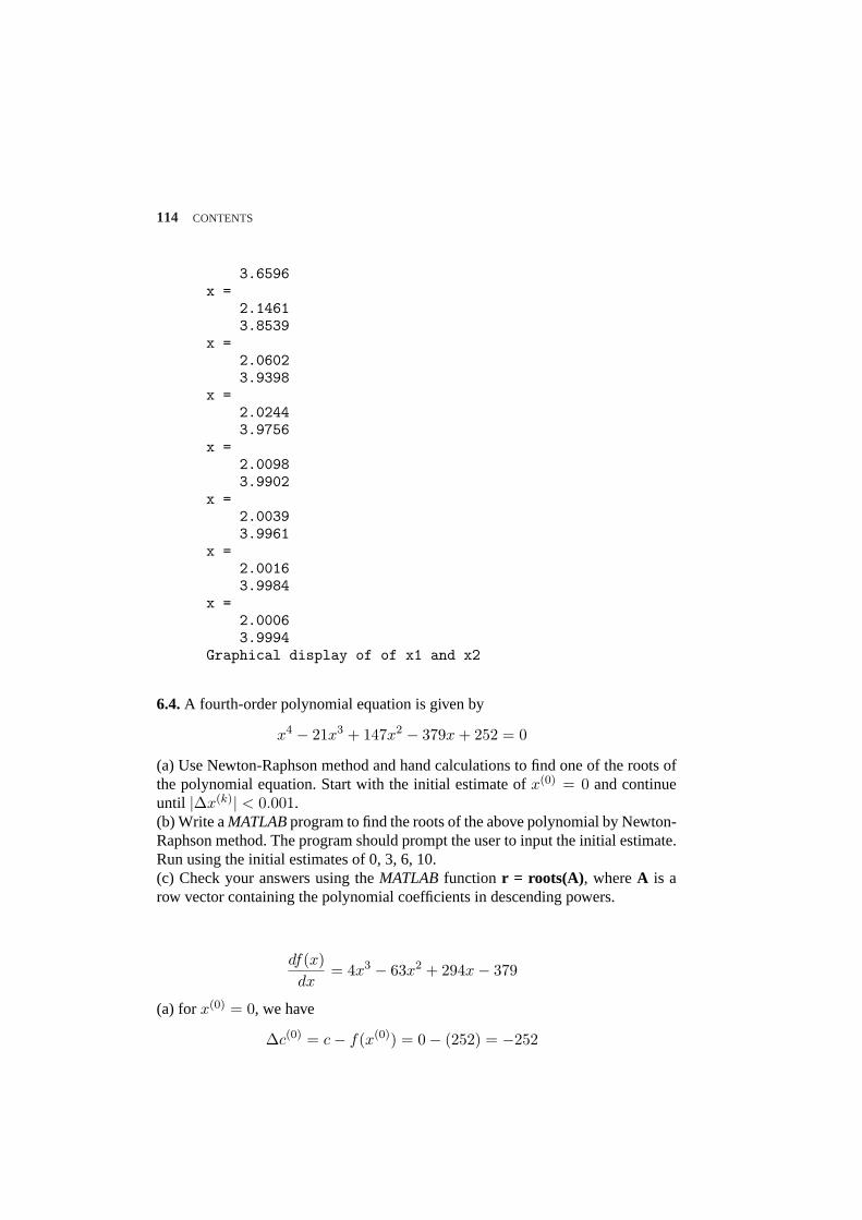
114 CONTENTS
3.6596x =
2.14613.8539
x =2.06023.9398
x =2.02443.9756
x =2.00983.9902
x =2.00393.9961
x =2.00163.9984
x =2.00063.9994
Graphical display of of x1 and x2
6.4.A fourth-order polynomial equation is given by
x4 − 21x3 + 147x2 − 379x + 252 = 0
(a) Use Newton-Raphson method and hand calculations to find one of the roots ofthe polynomial equation. Start with the initial estimate ofx(0) = 0 and continueuntil |∆x(k)| < 0.001.(b) Write aMATLABprogram to find the roots of the above polynomial by Newton-Raphson method. The program should prompt the user to input the initial estimate.Run using the initial estimates of 0, 3, 6, 10.(c) Check your answers using theMATLAB function r = roots(A) , whereA is arow vector containing the polynomial coefficients in descending powers.
df(x)dx
= 4x3 − 63x2 + 294x− 379
(a) forx(0) = 0, we have
∆c(0) = c− f(x(0)) = 0− (252) = −252
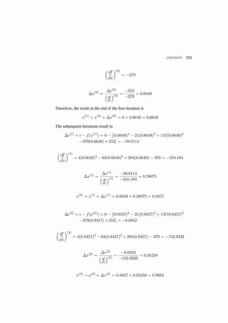
CONTENTS 115
(df
dx
)(0)
= −379
∆x(0) =∆c(0)
(dfdx
)(0)=−252−379
= 0.6649
Therefore, the result at the end of the first iteration is
x(1) = x(0) + ∆x(0) = 0 + 0.6649 = 0.6649
The subsequent iterations result in
∆c(1) = c− f(x(1)) = 0− [(0.6649)4 − 21(0.6649)3 + 147(0.6649)2
−379(0.6649) + 252] = −59.0114
(df
dx
)(1)
= 4(0.6649)3 − 63(0.6649)2 + 294(0.6649)− 379 = −210.194
∆x(1) =∆c(1)
(dfdx
)(1)=−59.0114−210.194
= 0.28075
x(2) = x(1) + ∆x(1) = 0.6649 + 0.28075 = 0.9457
∆c(2) = c− f(x(2)) = 0− [(0.9457)4 − 21(0.9457)3 + 147(0.9457)2
−379(0.9457) + 252] = −8.0942
(df
dx
)(2)
= 4(0.9457)3 − 63(0.9457)2 + 294(0.9457)− 379 = −153.9333
∆x(2) =∆c(2)
(dfdx
)(2)=
−8.0942−153.9333
= 0.05258
x(3) = x(2) + ∆x(2) = 0.9457 + 0.05258 = 0.9982
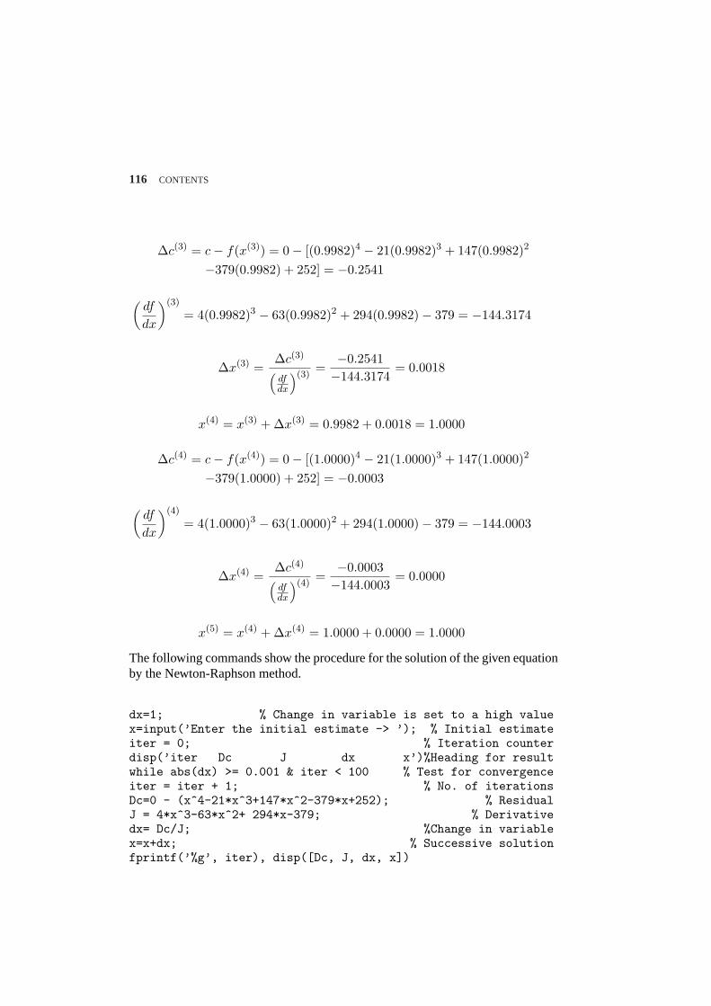
116 CONTENTS
∆c(3) = c− f(x(3)) = 0− [(0.9982)4 − 21(0.9982)3 + 147(0.9982)2
−379(0.9982) + 252] = −0.2541
(df
dx
)(3)
= 4(0.9982)3 − 63(0.9982)2 + 294(0.9982)− 379 = −144.3174
∆x(3) =∆c(3)
(dfdx
)(3)=
−0.2541−144.3174
= 0.0018
x(4) = x(3) + ∆x(3) = 0.9982 + 0.0018 = 1.0000
∆c(4) = c− f(x(4)) = 0− [(1.0000)4 − 21(1.0000)3 + 147(1.0000)2
−379(1.0000) + 252] = −0.0003
(df
dx
)(4)
= 4(1.0000)3 − 63(1.0000)2 + 294(1.0000)− 379 = −144.0003
∆x(4) =∆c(4)
(dfdx
)(4)=
−0.0003−144.0003
= 0.0000
x(5) = x(4) + ∆x(4) = 1.0000 + 0.0000 = 1.0000
The following commands show the procedure for the solution of the given equationby the Newton-Raphson method.
dx=1; % Change in variable is set to a high valuex=input(’Enter the initial estimate -> ’); % Initial estimateiter = 0; % Iteration counterdisp(’iter Dc J dx x’)%Heading for resultwhile abs(dx) >= 0.001 & iter < 100 % Test for convergenceiter = iter + 1; % No. of iterationsDc=0 - (x^4-21*x^3+147*x^2-379*x+252); % ResidualJ = 4*x^3-63*x^2+ 294*x-379; % Derivativedx= Dc/J; %Change in variablex=x+dx; % Successive solutionfprintf(’%g’, iter), disp([Dc, J, dx, x])
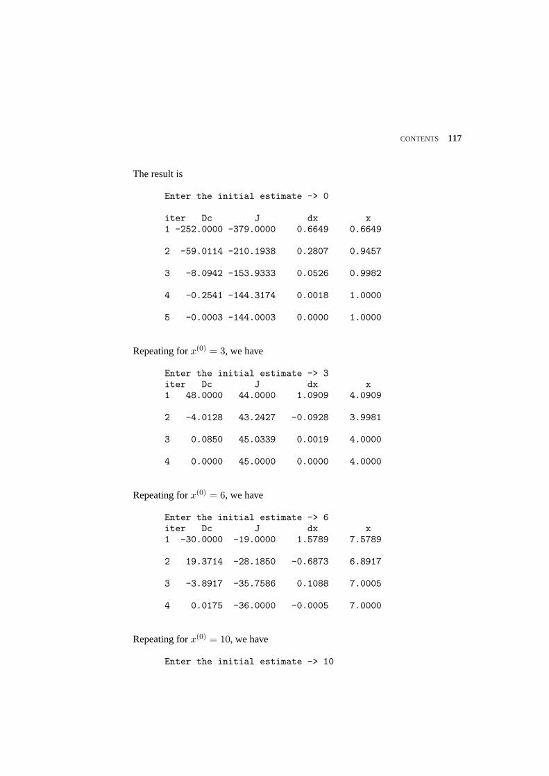
CONTENTS 117
The result is
Enter the initial estimate -> 0
iter Dc J dx x1 -252.0000 -379.0000 0.6649 0.6649
2 -59.0114 -210.1938 0.2807 0.9457
3 -8.0942 -153.9333 0.0526 0.9982
4 -0.2541 -144.3174 0.0018 1.0000
5 -0.0003 -144.0003 0.0000 1.0000
Repeating forx(0) = 3, we have
Enter the initial estimate -> 3iter Dc J dx x1 48.0000 44.0000 1.0909 4.0909
2 -4.0128 43.2427 -0.0928 3.9981
3 0.0850 45.0339 0.0019 4.0000
4 0.0000 45.0000 0.0000 4.0000
Repeating forx(0) = 6, we have
Enter the initial estimate -> 6iter Dc J dx x1 -30.0000 -19.0000 1.5789 7.5789
2 19.3714 -28.1850 -0.6873 6.8917
3 -3.8917 -35.7586 0.1088 7.0005
4 0.0175 -36.0000 -0.0005 7.0000
Repeating forx(0) = 10, we have
Enter the initial estimate -> 10
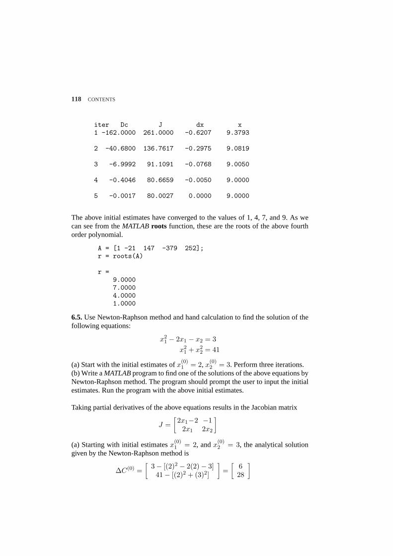
118 CONTENTS
iter Dc J dx x1 -162.0000 261.0000 -0.6207 9.3793
2 -40.6800 136.7617 -0.2975 9.0819
3 -6.9992 91.1091 -0.0768 9.0050
4 -0.4046 80.6659 -0.0050 9.0000
5 -0.0017 80.0027 0.0000 9.0000
The above initial estimates have converged to the values of 1, 4, 7, and 9. As wecan see from theMATLABroots function, these are the roots of the above fourthorder polynomial.
A = [1 -21 147 -379 252];r = roots(A)
r =9.00007.00004.00001.0000
6.5.Use Newton-Raphson method and hand calculation to find the solution of thefollowing equations:
x21 − 2x1 − x2 = 3
x21 + x2
2 = 41
(a) Start with the initial estimates ofx(0)1 = 2, x
(0)2 = 3. Perform three iterations.
(b) Write aMATLABprogram to find one of the solutions of the above equations byNewton-Raphson method. The program should prompt the user to input the initialestimates. Run the program with the above initial estimates.
Taking partial derivatives of the above equations results in the Jacobian matrix
J =[2x1−2 −1
2x1 2x2
]
(a) Starting with initial estimatesx(0)1 = 2, andx
(0)2 = 3, the analytical solution
given by the Newton-Raphson method is
∆C(0) =[
3− [(2)2 − 2(2)− 3]41− [(2)2 + (3)2]
]=
[628
]
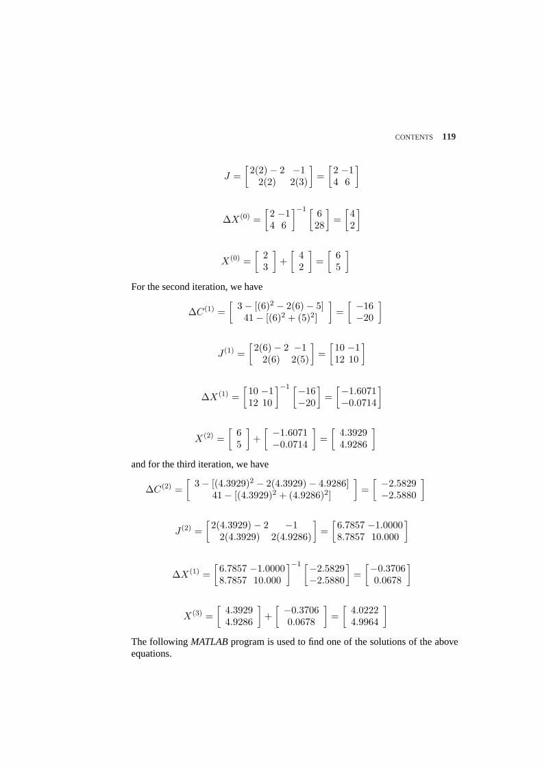
CONTENTS 119
J =[2(2)− 2 −1
2(2) 2(3)
]=
[2 −14 6
]
∆X(0) =[2 −14 6
]−1 [628
]=
[42
]
X(0) =[
23
]+
[42
]=
[65
]
For the second iteration, we have
∆C(1) =[
3− [(6)2 − 2(6)− 5]41− [(6)2 + (5)2]
]=
[ −16−20
]
J (1) =[2(6)− 2 −1
2(6) 2(5)
]=
[10 −112 10
]
∆X(1) =[10 −112 10
]−1 [−16−20
]=
[−1.6071−0.0714
]
X(2) =[
65
]+
[ −1.6071−0.0714
]=
[4.39294.9286
]
and for the third iteration, we have
∆C(2) =[
3− [(4.3929)2 − 2(4.3929)− 4.9286]41− [(4.3929)2 + (4.9286)2]
]=
[ −2.5829−2.5880
]
J (2) =[2(4.3929)− 2 −1
2(4.3929) 2(4.9286)
]=
[6.7857 −1.00008.7857 10.000
]
∆X(1) =[6.7857 −1.00008.7857 10.000
]−1 [−2.5829−2.5880
]=
[−0.37060.0678
]
X(3) =[
4.39294.9286
]+
[ −0.37060.0678
]=
[4.02224.9964
]
The followingMATLABprogram is used to find one of the solutions of the aboveequations.
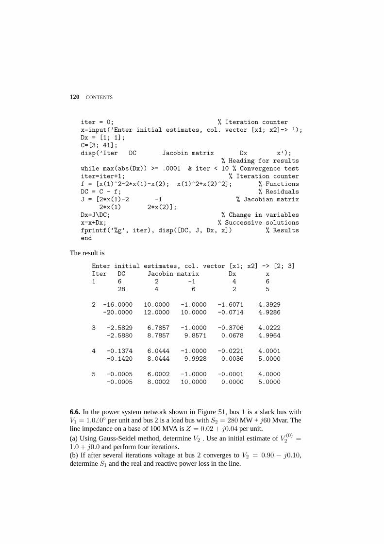
120 CONTENTS
iter = 0; % Iteration counterx=input(’Enter initial estimates, col. vector [x1; x2]-> ’);Dx = [1; 1];C=[3; 41];disp(’Iter DC Jacobin matrix Dx x’);
% Heading for resultswhile max(abs(Dx)) >= .0001 & iter < 10 % Convergence testiter=iter+1; % Iteration counterf = [x(1)^2-2*x(1)-x(2); x(1)^2+x(2)^2]; % FunctionsDC = C - f; % ResidualsJ = [2*x(1)-2 -1 % Jacobian matrix
2*x(1) 2*x(2)];Dx=J\DC; % Change in variablesx=x+Dx; % Successive solutionsfprintf(’%g’, iter), disp([DC, J, Dx, x]) % Resultsend
The result is
Enter initial estimates, col. vector [x1; x2] -> [2; 3]Iter DC Jacobin matrix Dx x1 6 2 -1 4 6
28 4 6 2 5
2 -16.0000 10.0000 -1.0000 -1.6071 4.3929-20.0000 12.0000 10.0000 -0.0714 4.9286
3 -2.5829 6.7857 -1.0000 -0.3706 4.0222-2.5880 8.7857 9.8571 0.0678 4.9964
4 -0.1374 6.0444 -1.0000 -0.0221 4.0001-0.1420 8.0444 9.9928 0.0036 5.0000
5 -0.0005 6.0002 -1.0000 -0.0001 4.0000-0.0005 8.0002 10.0000 0.0000 5.0000
6.6. In the power system network shown in Figure 51, bus 1 is a slack bus withV1 = 1.06 0 per unit and bus 2 is a load bus withS2 = 280 MW + j60 Mvar. Theline impedance on a base of 100 MVA isZ = 0.02 + j0.04 per unit.(a) Using Gauss-Seidel method, determineV2 . Use an initial estimate ofV (0)
2 =1.0 + j0.0 and perform four iterations.(b) If after several iterations voltage at bus 2 converges toV2 = 0.90 − j0.10,determineS1 and the real and reactive power loss in the line.
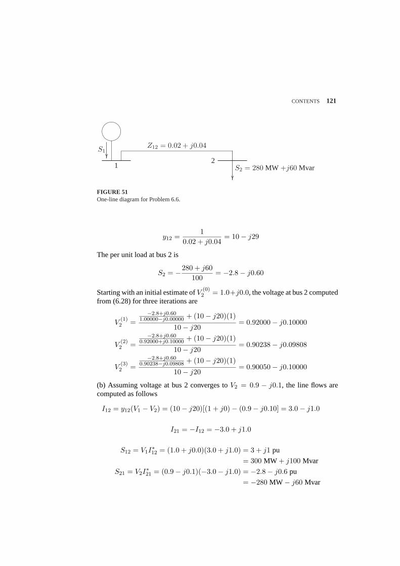
CONTENTS 121
½¼
¾»
.....................................................................................................................
........
........
........
...................................................................
........
........
........S1
12
Z12 = 0.02 + j0.04
S2 = 280 MW +j60 Mvar
FIGURE 51One-line diagram for Problem 6.6.
y12 =1
0.02 + j0.04= 10− j29
The per unit load at bus 2 is
S2 = −280 + j60100
= −2.8− j0.60
Starting with an initial estimate ofV (0)2 = 1.0+j0.0, the voltage at bus 2 computed
from (6.28) for three iterations are
V(1)2 =
−2.8+j0.601.00000−j0.00000 + (10− j20)(1)
10− j20= 0.92000− j0.10000
V(2)2 =
−2.8+j0.600.92000+j0.10000 + (10− j20)(1)
10− j20= 0.90238− j0.09808
V(3)2 =
−2.8+j0.600.90238−j0.09808 + (10− j20)(1)
10− j20= 0.90050− j0.10000
(b) Assuming voltage at bus 2 converges toV2 = 0.9 − j0.1, the line flows arecomputed as follows
I12 = y12(V1 − V2) = (10− j20)[(1 + j0)− (0.9− j0.10] = 3.0− j1.0
I21 = −I12 = −3.0 + j1.0
S12 = V1I∗12 = (1.0 + j0.0)(3.0 + j1.0) = 3 + j1 pu
= 300 MW + j100 Mvar
S21 = V2I∗21 = (0.9− j0.1)(−3.0− j1.0) = −2.8− j0.6 pu
= −280 MW − j60 Mvar
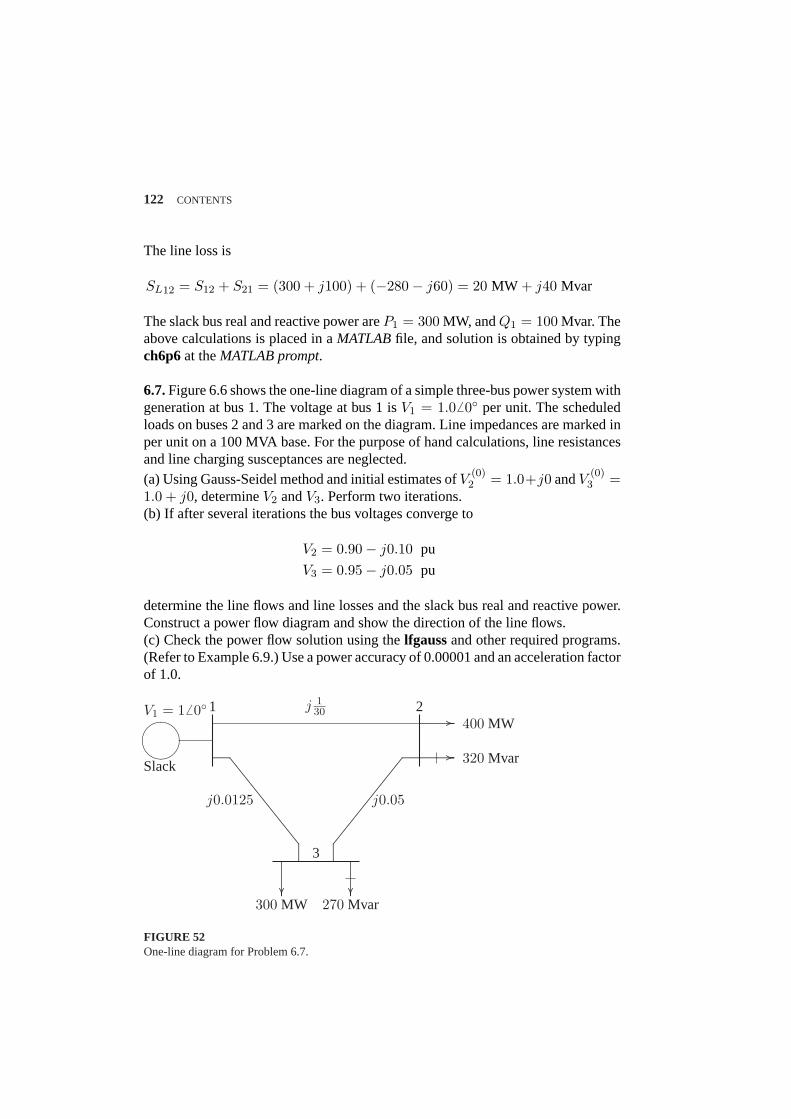
122 CONTENTS
The line loss is
SL12 = S12 + S21 = (300 + j100) + (−280− j60) = 20 MW + j40 Mvar
The slack bus real and reactive power areP1 = 300 MW, andQ1 = 100 Mvar. Theabove calculations is placed in aMATLABfile, and solution is obtained by typingch6p6at theMATLAB prompt.
6.7.Figure 6.6 shows the one-line diagram of a simple three-bus power system withgeneration at bus 1. The voltage at bus 1 isV1 = 1.0 6 0 per unit. The scheduledloads on buses 2 and 3 are marked on the diagram. Line impedances are marked inper unit on a 100 MVA base. For the purpose of hand calculations, line resistancesand line charging susceptances are neglected.(a) Using Gauss-Seidel method and initial estimates ofV
(0)2 = 1.0+j0 andV
(0)3 =
1.0 + j0, determineV2 andV3. Perform two iterations.(b) If after several iterations the bus voltages converge to
V2 = 0.90− j0.10 pu
V3 = 0.95− j0.05 pu
determine the line flows and line losses and the slack bus real and reactive power.Construct a power flow diagram and show the direction of the line flows.(c) Check the power flow solution using thelfgaussand other required programs.(Refer to Example 6.9.) Use a power accuracy of 0.00001 and an acceleration factorof 1.0.
½¼
¾»
................................................................................................................................................................................................................................................................................... ...................................................................................................................................................................................................................................................................................
.................................................................................. ................
.................................................................................. ................
..........................................................................
........
........
........
..........................................................................
........
........
........
j 130
j0.0125 j0.05
1 2
3
400 MW
320 Mvar
300 MW 270 Mvar
Slack
V1 = 1 6 0
FIGURE 52One-line diagram for Problem 6.7.

CONTENTS 123
(a) Line impedances are converted to admittances
y12 = −j30
y13 =1
j0.0125= −j80
y23 =1
j0.05= −j20
At the P-Q buses, the complex loads expressed in per units are
Ssch2 = −(400 + j320)
100= −4.0− j3.2 pu
Ssch3 = −(300 + j270)
100= −3.0− j2.7 pu
For hand calculation, we use (6.28). Bus 1 is taken as reference bus (slack bus).Starting from an initial estimate ofV (0)
2 = 1.0 + j0.0 andV(0)3 = 1.0 + j0.0, V2
andV3 are computed from (6.28) as follows
V(1)2 =
Ssch2
∗
V(0)2
∗ + y12V1 + y23V(0)3
y12 + y23
=−4.0+j3.2
1.0−j0 + (−j30)(1.0 + j0) + (−j20)(1.0 + j0)
−j50= 0.936− j0.08
and
V(1)3 =
Ssch3
∗
V(0)3
∗ + y13V1 + y23V(1)2
y13 + y23
=−3.0+j2.7
1−j0 + (−j80)(1.0 + j0) + (−j20)(0.936− j0.08)
−j100= 0.9602− j0.046
For the second iteration we have
V(2)2 =
−4.0+j3.20.936+j0.08 + (−j30)(1.0 + j0) + (−j20)(0.9602− j0.046)
−j50= 0.9089− j0.0974
and
V(2)3 =
−3.0+j2.70.9602+j0.046 + (−j80)(1.0 + j0) + (−j20)(0.9089− j0.0974)
(−j100)= 0.9522− j0.0493
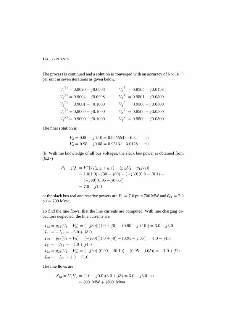
124 CONTENTS
The process is continued and a solution is converged with an accuracy of5× 10−5
per unit in seven iterations as given below.
V(3)2 = 0.9020− j0.0993 V
(3)3 = 0.9505− j0.0498
V(4)2 = 0.9004− j0.0998 V
(4)3 = 0.9501− j0.0500
V(5)2 = 0.9001− j0.1000 V
(5)3 = 0.9500− j0.0500
V(6)2 = 0.9000− j0.1000 V
(6)3 = 0.9500− j0.0500
V(7)2 = 0.9000− j0.1000 V
(7)3 = 0.9500− j0.0500
The final solution is
V2 = 0.90− j0.10 = 0.9055546 −6.34 pu
V3 = 0.95− j0.05 = 0.95136 −3.0128 pu
(b) With the knowledge of all bus voltages, the slack bus power is obtained from(6.27)
P1 − jQ1 = V ∗1 [V1(y12 + y13)− (y12V2 + y13V3)]
= 1.0[1.0(−j30− j80)− (−j30)(0.9− j0.1)−(−j80)(0.95− j0.05)]
= 7.0− j7.0
or the slack bus real and reactive powers areP1 = 7.0 pu = 700 MW andQ1 = 7.0pu= 700 Mvar.
To find the line flows, first the line currents are computed. With line charging ca-pacitors neglected, the line currents are
I12 = y12(V1 − V2) = (−j30)[(1.0 + j0)− (0.90− j0.10)] = 3.0− j3.0I21 = −I12 = −3.0 + j3.0I13 = y13(V1 − V3) = (−j80)[(1.0 + j0)− (0.95− j.05)] = 4.0− j4.0I31 = −I13 = −4.0 + j4.0I23 = y23(V2 − V3) = (−j20)[(0.90− j0.10)− (0.95− j.05)] = −1.0 + j1.0I32 = −I23 = 1.0− j1.0
The line flows are
S12 = V1I∗12 = (1.0 + j0.0)(3.0 + j3) = 3.0 + j3.0 pu
= 300 MW + j300 Mvar
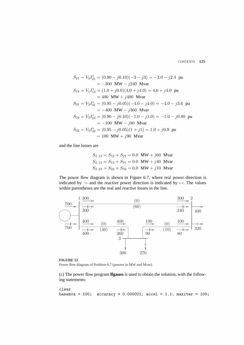
CONTENTS 125
S21 = V2I∗21 = (0.90− j0.10)(−3− j3) = −3.0− j2.4 pu
= −300 MW − j240 Mvar
S13 = V1I∗13 = (1.0 + j0.0)(4.0 + j4.0) = 4.0 + j4.0 pu
= 400 MW + j400 Mvar
S31 = V3I∗31 = (0.95− j0.05)(−4.0− j4.0) = −4.0− j3.6 pu
= −400 MW − j360 Mvar
S23 = V2I∗23 = (0.90− j0.10)(−1.0− j1.0) = −1.0− j0.80 pu
= −100 MW − j80 Mvar
S32 = V3I∗32 = (0.95− j0.05)(1 + j1) = 1.0 + j0.9 pu
= 100 MW + j90 Mvar
and the line losses are
SL 12 = S12 + S21 = 0.0 MW + j60 Mvar
SL 13 = S13 + S31 = 0.0 MW + j40 Mvar
SL 23 = S23 + S32 = 0.0 MW + j10 Mvar
The power flow diagram is shown in Figure 6.7, where real power direction isindicated by→ and the reactive power direction is indicated by7→. The valueswithin parentheses are the real and reactive losses in the line.
½¼
¾»
...............................................................................
........
........
........
...............................................................................
........
........
........
....................................................................................... ................
....................................................................................... ................
(0)(60)
(0)(40)
(0)(10)
400
320
300 270
1 2
3
700....................................................................................... ................
....................................................................................... ................
700
300....................................................................................... ................
....................................................................................... ................
300
300....................................................................................... ................
....................................................................................... ................
240
400....................................................................................... ................
....................................................................................... ................
400
400..................................................................... ................
..................................................................... ................
360
100..................................................................... ................
..................................................................... ................
90
100....................................................................................... ................
....................................................................................... ................
80
FIGURE 53Power flow diagram of Problem 6.7 (powers in MW and Mvar).
(c) The power flow programlfgaussis used to obtain the solution, with the follow-ing statements:
clearbasemva = 100; accuracy = 0.000001; accel = 1.1; maxiter = 100;
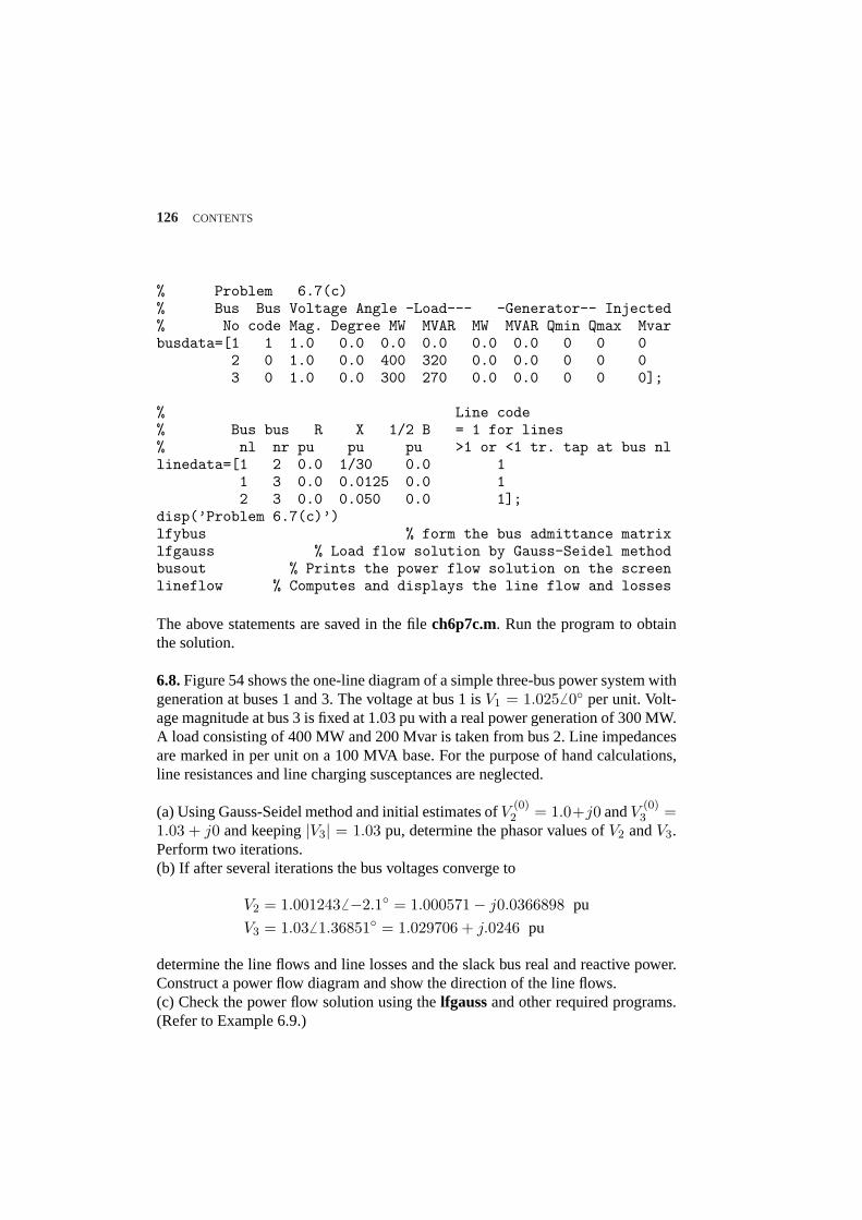
126 CONTENTS
% Problem 6.7(c)% Bus Bus Voltage Angle -Load--- -Generator-- Injected% No code Mag. Degree MW MVAR MW MVAR Qmin Qmax Mvarbusdata=[1 1 1.0 0.0 0.0 0.0 0.0 0.0 0 0 0
2 0 1.0 0.0 400 320 0.0 0.0 0 0 03 0 1.0 0.0 300 270 0.0 0.0 0 0 0];
% Line code% Bus bus R X 1/2 B = 1 for lines% nl nr pu pu pu >1 or <1 tr. tap at bus nllinedata=[1 2 0.0 1/30 0.0 1
1 3 0.0 0.0125 0.0 12 3 0.0 0.050 0.0 1];
disp(’Problem 6.7(c)’)lfybus % form the bus admittance matrixlfgauss % Load flow solution by Gauss-Seidel methodbusout % Prints the power flow solution on the screenlineflow % Computes and displays the line flow and losses
The above statements are saved in the filech6p7c.m. Run the program to obtainthe solution.
6.8.Figure 54 shows the one-line diagram of a simple three-bus power system withgeneration at buses 1 and 3. The voltage at bus 1 isV1 = 1.0256 0 per unit. Volt-age magnitude at bus 3 is fixed at 1.03 pu with a real power generation of 300 MW.A load consisting of 400 MW and 200 Mvar is taken from bus 2. Line impedancesare marked in per unit on a 100 MVA base. For the purpose of hand calculations,line resistances and line charging susceptances are neglected.
(a) Using Gauss-Seidel method and initial estimates ofV(0)2 = 1.0+j0 andV
(0)3 =
1.03 + j0 and keeping|V3| = 1.03 pu, determine the phasor values ofV2 andV3.Perform two iterations.(b) If after several iterations the bus voltages converge to
V2 = 1.0012436 −2.1 = 1.000571− j0.0366898 pu
V3 = 1.036 1.36851 = 1.029706 + j.0246 pu
determine the line flows and line losses and the slack bus real and reactive power.Construct a power flow diagram and show the direction of the line flows.(c) Check the power flow solution using thelfgaussand other required programs.(Refer to Example 6.9.)
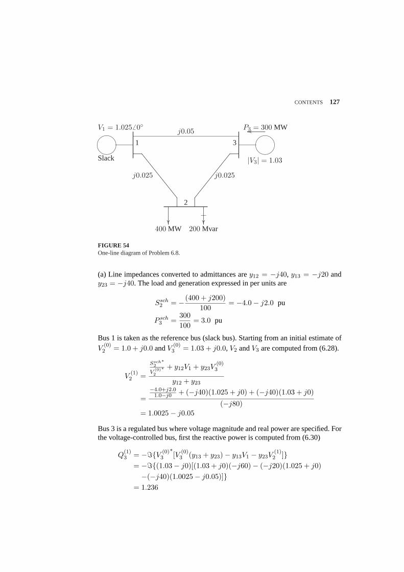
CONTENTS 127
½¼
¾»
½¼
¾»
................................................................................................................................................................................................................................................................................... ...................................................................................................................................................................................................................................................................................
..................................................................................................
..........................................................................
........
........
........
..........................................................................
........
........
........
j0.05
j0.025 j0.025
1 3
2
P3 = 300 MW
400 MW 200 Mvar
Slack
V1 = 1.0256 0
|V3| = 1.03
FIGURE 54One-line diagram of Problem 6.8.
(a) Line impedances converted to admittances arey12 = −j40, y13 = −j20 andy23 = −j40. The load and generation expressed in per units are
Ssch2 = −(400 + j200)
100= −4.0− j2.0 pu
P sch3 =
300100
= 3.0 pu
Bus 1 is taken as the reference bus (slack bus). Starting from an initial estimate ofV
(0)2 = 1.0 + j0.0 andV
(0)3 = 1.03 + j0.0, V2 andV3 are computed from (6.28).
V(1)2 =
Ssch2
∗
V(0)2
∗ + y12V1 + y23V(0)3
y12 + y23
=−4.0+j2.0
1.0−j0 + (−j40)(1.025 + j0) + (−j40)(1.03 + j0)
(−j80)= 1.0025− j0.05
Bus 3 is a regulated bus where voltage magnitude and real power are specified. Forthe voltage-controlled bus, first the reactive power is computed from (6.30)
Q(1)3 = −=V (0)
3
∗[V (0)
3 (y13 + y23)− y13V1 − y23V(1)2 ]
= −=(1.03− j0)[(1.03 + j0)(−j60)− (−j20)(1.025 + j0)−(−j40)(1.0025− j0.05)]
= 1.236
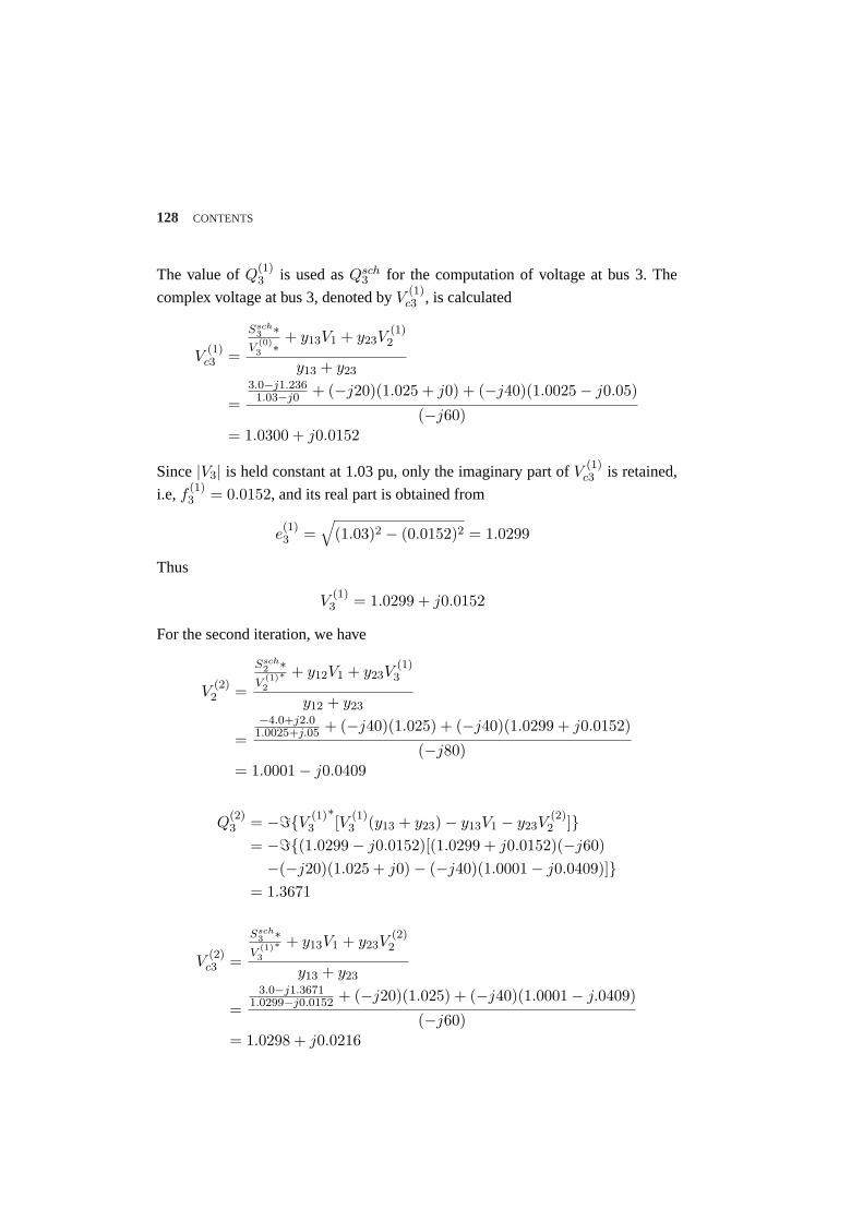
128 CONTENTS
The value ofQ(1)3 is used asQsch
3 for the computation of voltage at bus 3. The
complex voltage at bus 3, denoted byV(1)c3 , is calculated
V(1)c3 =
Ssch3 ∗
V(0)3 ∗ + y13V1 + y23V
(1)2
y13 + y23
=3.0−j1.2361.03−j0 + (−j20)(1.025 + j0) + (−j40)(1.0025− j0.05)
(−j60)= 1.0300 + j0.0152
Since|V3| is held constant at 1.03 pu, only the imaginary part ofV(1)c3 is retained,
i.e,f (1)3 = 0.0152, and its real part is obtained from
e(1)3 =
√(1.03)2 − (0.0152)2 = 1.0299
Thus
V(1)3 = 1.0299 + j0.0152
For the second iteration, we have
V(2)2 =
Ssch2 ∗
V(1)2
∗ + y12V1 + y23V(1)3
y12 + y23
=−4.0+j2.01.0025+j.05 + (−j40)(1.025) + (−j40)(1.0299 + j0.0152)
(−j80)= 1.0001− j0.0409
Q(2)3 = −=V (1)
3
∗[V (1)
3 (y13 + y23)− y13V1 − y23V(2)2 ]
= −=(1.0299− j0.0152)[(1.0299 + j0.0152)(−j60)−(−j20)(1.025 + j0)− (−j40)(1.0001− j0.0409)]
= 1.3671
V(2)c3 =
Ssch3 ∗
V(1)3
∗ + y13V1 + y23V(2)2
y13 + y23
=3.0−j1.3671
1.0299−j0.0152 + (−j20)(1.025) + (−j40)(1.0001− j.0409)
(−j60)= 1.0298 + j0.0216
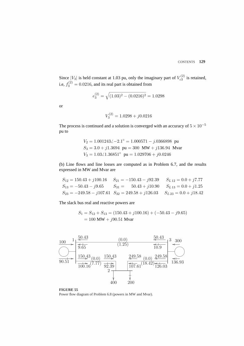
CONTENTS 129
Since|V3| is held constant at 1.03 pu, only the imaginary part ofV(2)c3 is retained,
i.e,f (2)3 = 0.0216, and its real part is obtained from
e(2)3 =
√(1.03)2 − (0.0216)2 = 1.0298
or
V(2)3 = 1.0298 + j0.0216
The process is continued and a solution is converged with an accuracy of5× 10−5
pu to
V2 = 1.0012436 −2.1 = 1.000571− j.0366898 pu
S3 = 3.0 + j1.3694 pu = 300 MW + j136.94 Mvar
V3 = 1.036 1.36851 pu = 1.029706 + j0.0246
(b) Line flows and line losses are computed as in Problem 6.7, and the resultsexpressed in MW and Mvar are
S12 = 150.43 + j100.16 S21 = −150.43− j92.39 SL 12 = 0.0 + j7.77S13 = −50.43− j9.65 S31 = 50.43 + j10.90 SL 13 = 0.0 + j1.25S23 = −249.58− j107.61 S32 = 249.58 + j126.03 SL 23 = 0.0 + j18.42
The slack bus real and reactive powers are
S1 = S12 + S13 = (150.43 + j100.16) + (−50.43− j9.65)= 100 MW + j90.51 Mvar
¹¸
º·
¹¸
º·............................................................................
300
............................................................................
136.93
..................................................................
........
........
........
400
..................................................................
........
........
........
200
(0.0)(1.25)
(0.0)(7.77)
(0.0)(18.42)
1 3
2
100....................................................................................................... ................
....................................................................................................... ................
90.51
50.43..........................................................................................
..........................................................................................
9.65
50.43.........................................................................................................
.........................................................................................................
10.9
150.43.......................................................................... ................
.......................................................................... ................
100.16
150.43.......................................................................... ................
.......................................................................... ................
92.39
249.58...................................................................................
...................................................................................
107.61
249.58..................................................................................................
..................................................................................................
126.03
FIGURE 55Power flow diagram of Problem 6.8 (powers in MW and Mvar).
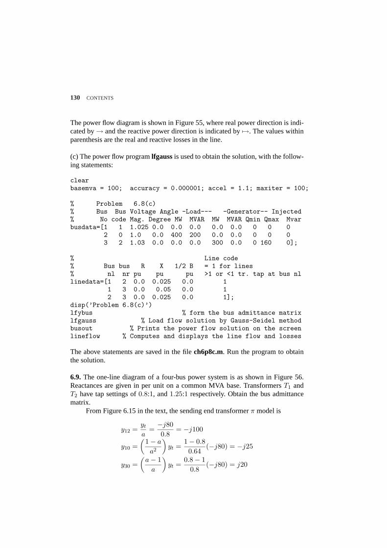
130 CONTENTS
The power flow diagram is shown in Figure 55, where real power direction is indi-cated by→ and the reactive power direction is indicated by7→. The values withinparenthesis are the real and reactive losses in the line.
(c) The power flow programlfgaussis used to obtain the solution, with the follow-ing statements:
clearbasemva = 100; accuracy = 0.000001; accel = 1.1; maxiter = 100;
% Problem 6.8(c)% Bus Bus Voltage Angle -Load--- -Generator-- Injected% No code Mag. Degree MW MVAR MW MVAR Qmin Qmax Mvarbusdata=[1 1 1.025 0.0 0.0 0.0 0.0 0.0 0 0 0
2 0 1.0 0.0 400 200 0.0 0.0 0 0 03 2 1.03 0.0 0.0 0.0 300 0.0 0 160 0];
% Line code% Bus bus R X 1/2 B = 1 for lines% nl nr pu pu pu >1 or <1 tr. tap at bus nllinedata=[1 2 0.0 0.025 0.0 1
1 3 0.0 0.05 0.0 12 3 0.0 0.025 0.0 1];
disp(’Problem 6.8(c)’)lfybus % form the bus admittance matrixlfgauss % Load flow solution by Gauss-Seidel methodbusout % Prints the power flow solution on the screenlineflow % Computes and displays the line flow and losses
The above statements are saved in the filech6p8c.m. Run the program to obtainthe solution.
6.9. The one-line diagram of a four-bus power system is as shown in Figure 56.Reactances are given in per unit on a common MVA base. TransformersT1 andT2 have tap settings of0.8:1, and1.25:1 respectively. Obtain the bus admittancematrix.
From Figure 6.15 in the text, the sending end transformerπ model is
y12 =yt
a=−j800.8
= −j100
y10 =(
1− a
a2
)yt =
1− 0.80.64
(−j80) = −j25
y30 =(
a− 1a
)yt =
0.8− 10.8
(−j80) = j20
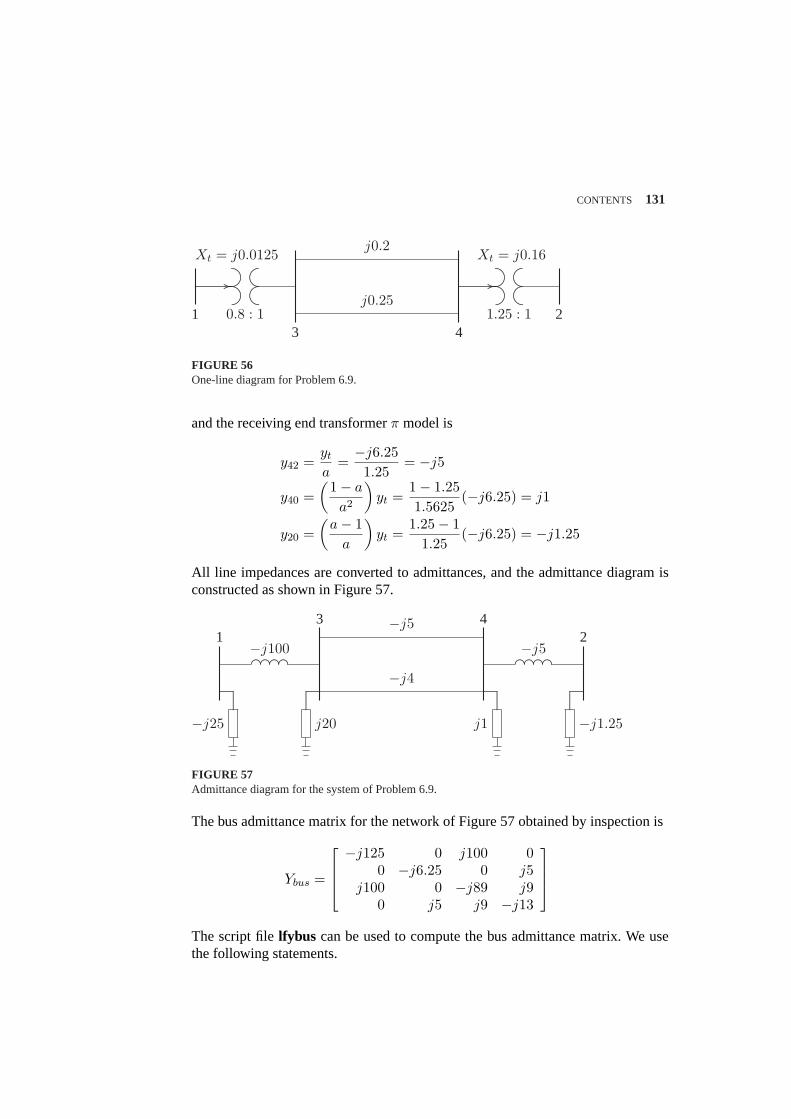
CONTENTS 131
..................................................................................... ................ ..................................................................................... ................
............................................................................................................ ............................................................................................................ ............................................................................................................ .................
...........................................................................................
Xt = j0.0125 Xt = j0.16j0.2
j0.251
3 420.8 : 1 1.25 : 1
FIGURE 56One-line diagram for Problem 6.9.
and the receiving end transformerπ model is
y42 =yt
a=−j6.251.25
= −j5
y40 =(
1− a
a2
)yt =
1− 1.251.5625
(−j6.25) = j1
y20 =(
a− 1a
)yt =
1.25− 11.25
(−j6.25) = −j1.25
All line impedances are converted to admittances, and the admittance diagram isconstructed as shown in Figure 57.
.....................................
......................................................
................. .....................................
......................................................
.................
−j100 −j5
−j5
−j4
13 4
2
.............................................................
.............................................................
.............................................................
.............................................................
−j25 j20 j1 −j1.25
FIGURE 57Admittance diagram for the system of Problem 6.9.
The bus admittance matrix for the network of Figure 57 obtained by inspection is
Ybus =
−j125 0 j100 00 −j6.25 0 j5
j100 0 −j89 j90 j5 j9 −j13
The script filelfybus can be used to compute the bus admittance matrix. We usethe following statements.
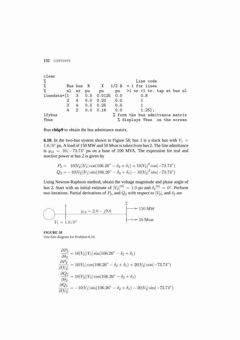
132 CONTENTS
clear% Line code% Bus bus R X 1/2 B = 1 for lines% nl nr pu pu pu >1 or <1 tr. tap at bus nllinedata=[1 3 0.0 0.0125 0.0 0.8
3 4 0.0 0.20 0.0 13 4 0.0 0.25 0.0 14 2 0.0 0.16 0.0 1.25];
lfybus % form the bus admittance matrixYbus % displays Ybus on the screen
Runch6p9to obtain the bus admittance matrix.
6.10. In the two-bus system shown in Figure 58, bus 1 is a slack bus withV1 =1.0 6 0 pu. A load of 150 MW and 50 Mvar is taken from bus 2. The line admittanceis y12 = 106 −73.74 pu on a base of 100 MVA. The expression for real andreactive power at bus 2 is given by
P2 = 10|V2||V1| cos(106.26 − δ2 + δ1) + 10|V2|2 cos(−73.74)Q2 = −10|V2||V1| sin(106.26 − δ2 + δ1)− 10|V2|2 sin(−73.74)
Using Newton-Raphson method, obtain the voltage magnitude and phase angle ofbus 2. Start with an initial estimate of|V2|(0) = 1.0 pu andδ2
(0) = 0. Performtwo iterations. Partial derivatives ofP2, andQ2 with respect to|V2|, andδ2 are
½¼
¾» ..................................................................................... ................
..................................................................................... ................
y12 = 2.8− j9.6
V1 = 1.0 6 0
150 MW
50 Mvar
12
FIGURE 58One-line diagram for Problem 6.10.
∂P2
∂δ2= 10|V2||V1| sin(106.26 − δ2 + δ1)
∂P2
∂|V2| = 10|V1| cos(106.26 − δ2 + δ1) + 20|V2| cos(−73.74)
∂Q2
∂δ2= 10|V2||V1| cos(106.26 − δ2 + δ1)
∂Q2
∂|V2| = −10|V1| sin(106.26 − δ2 + δ1)− 20|V2| sin(−73.74)
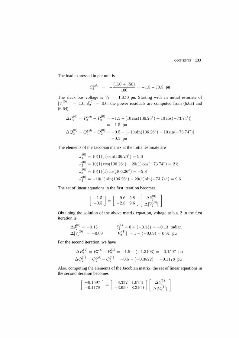
CONTENTS 133
The load expressed in per unit is
Ssch2 = −(150 + j50)
100= −1.5− j0.5 pu
The slack bus voltage isV1 = 1.06 0 pu. Starting with an initial estimate of|V (0)
2 | = 1.0, δ(0)2 = 0.0, the power residuals are computed from (6.63) and
(6.64)
∆P(0)2 = P sch
2 − P(0)2 = −1.5− [10 cos(106.26) + 10 cos(−73.74)]
= −1.5 pu
∆Q(0)2 = Qsch
2 −Q(0)2 = −0.5− [−10 sin(106.26)− 10 sin(−73.74)]
= −0.5 pu
The elements of the Jacobian matrix at the initial estimate are
J(0)1 = 10(1)(1) sin(106.26) = 9.6
J(0)2 = 10(1) cos(106.26) + 20(1) cos(−73.74) = 2.8
J(0)3 = 10(1)(1) cos(106.26) = −2.8
J(0)4 = −10(1) sin(106.26)− 20(1) sin(−73.74) = 9.6
The set of linear equations in the first iteration becomes
[ −1.5−0.5
]=
[9.6 2.8
−2.8 9.6
] [∆δ
(0)2
∆|V (0)2 |
]
Obtaining the solution of the above matrix equation, voltage at bus 2 in the firstiteration is
∆δ(0)2 = −0.13 δ
(1)2 = 0 + (−0.13) = −0.13 radian
∆|V (0)2 | = −0.09 |V (1)
2 | = 1 + (−0.09) = 0.91 pu
For the second iteration, we have
∆P(1)2 = P sch
2 − P(1)2 = −1.5− (−1.3403) = −0.1597 pu
∆Q(1)2 = Qsch
2 −Q(1)2 = −0.5− (−0.3822) = −0.1178 pu
Also, computing the elements of the Jacobian matrix, the set of linear equations inthe second iteration becomes
[ −0.1597−0.1178
]=
[8.332 1.0751
−3.659 8.3160
] [∆δ
(1)2
∆|V (1)2 |
]
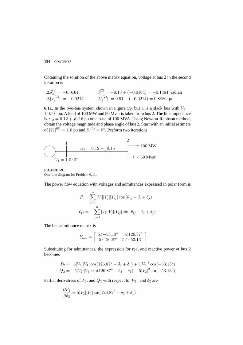
134 CONTENTS
Obtaining the solution of the above matrix equation, voltage at bus 2 in the seconditeration is
∆δ(1)2 = −0.0164 δ
(2)2 = −0.13 + (−0.0164) = −0.1464 radian
∆|V (1)2 | = −0.0214 |V (2)
2 | = 0.91 + (−0.0214) = 0.8886 pu
6.11. In the two-bus system shown in Figure 59, bus 1 is a slack bus withV1 =1.0 6 0 pu. A load of 100 MW and 50 Mvar is taken from bus 2. The line impedanceis z12 = 0.12 + j0.16 pu on a base of 100 MVA. Using Newton-Raphson method,obtain the voltage magnitude and phase angle of bus 2. Start with an initial estimateof |V2|(0) = 1.0 pu andδ2
(0) = 0. Perform two iterations.
½¼
¾» ..................................................................................... ................
..................................................................................... ................
z12 = 0.12 + j0.16
V1 = 1.0 6 0
100 MW
50 Mvar
12
FIGURE 59One-line diagram for Problem 6.11.
The power flow equation with voltages and admittances expressed in polar form is
Pi =n∑
j=1
|Vi||Vj ||Yij | cos (θij − δi + δj)
Qi = −n∑
j=1
|Vi||Vj ||Yij | sin (θij − δi + δj)
The bus admittance matrix is
Ybus =[
56 −53.13 56 126.8756 126.87 5 6 −53.13
]
Substituting for admittances, the expression for real and reactive power at bus 2becomes
P2 = 5|V2||V1| cos(126.87 − δ2 + δ1) + 5|V2|2 cos(−53.13)Q2 = −5|V2||V1| sin(126.87 − δ2 + δ1)− 5|V2|2 sin(−53.13)
Partial derivatives ofP2, andQ2 with respect to|V2|, andδ2 are
∂P2
∂δ2= 5|V2||V1| sin(126.87 − δ2 + δ1)
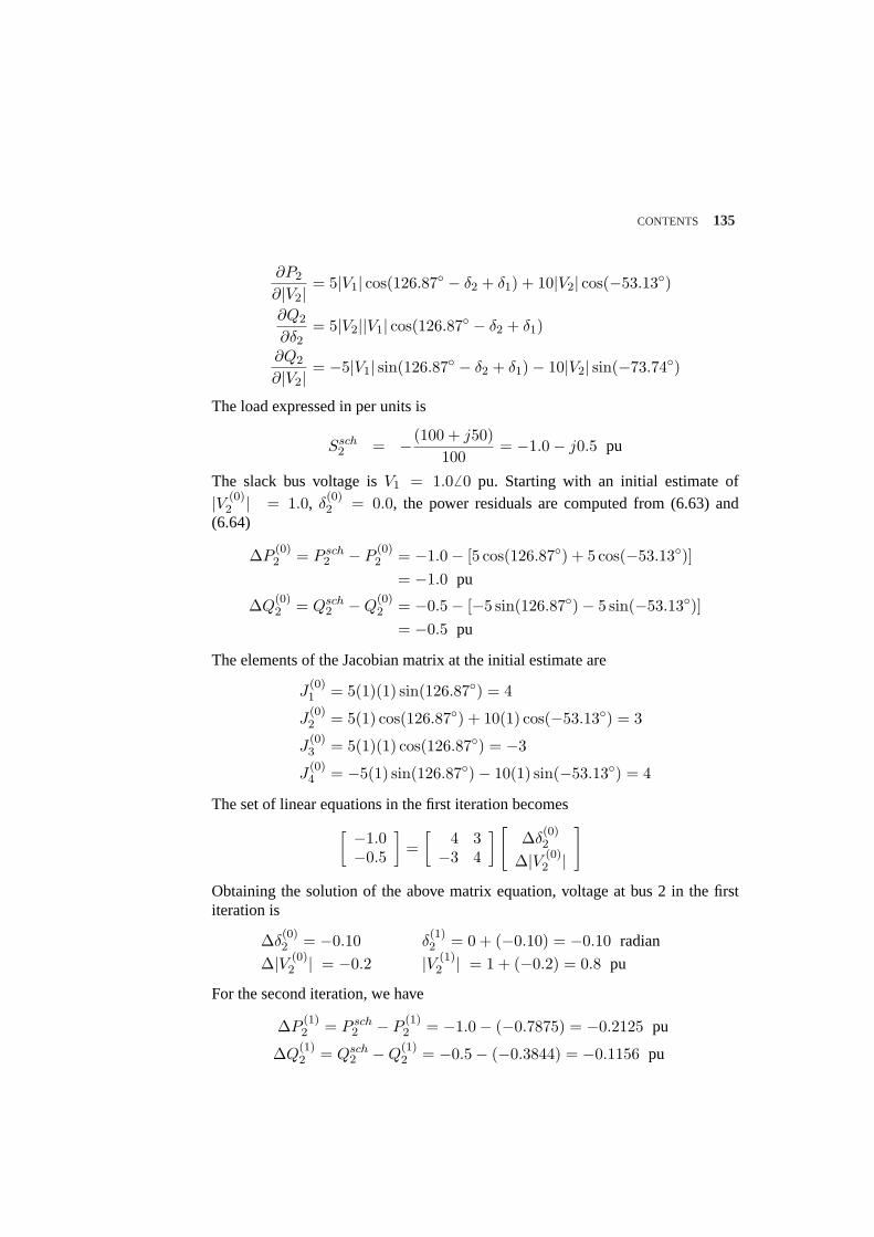
CONTENTS 135
∂P2
∂|V2| = 5|V1| cos(126.87 − δ2 + δ1) + 10|V2| cos(−53.13)
∂Q2
∂δ2= 5|V2||V1| cos(126.87 − δ2 + δ1)
∂Q2
∂|V2| = −5|V1| sin(126.87 − δ2 + δ1)− 10|V2| sin(−73.74)
The load expressed in per units is
Ssch2 = −(100 + j50)
100= −1.0− j0.5 pu
The slack bus voltage isV1 = 1.06 0 pu. Starting with an initial estimate of|V (0)
2 | = 1.0, δ(0)2 = 0.0, the power residuals are computed from (6.63) and
(6.64)
∆P(0)2 = P sch
2 − P(0)2 = −1.0− [5 cos(126.87) + 5 cos(−53.13)]
= −1.0 pu
∆Q(0)2 = Qsch
2 −Q(0)2 = −0.5− [−5 sin(126.87)− 5 sin(−53.13)]
= −0.5 pu
The elements of the Jacobian matrix at the initial estimate are
J(0)1 = 5(1)(1) sin(126.87) = 4
J(0)2 = 5(1) cos(126.87) + 10(1) cos(−53.13) = 3
J(0)3 = 5(1)(1) cos(126.87) = −3
J(0)4 = −5(1) sin(126.87)− 10(1) sin(−53.13) = 4
The set of linear equations in the first iteration becomes
[ −1.0−0.5
]=
[4 3
−3 4
] [∆δ
(0)2
∆|V (0)2 |
]
Obtaining the solution of the above matrix equation, voltage at bus 2 in the firstiteration is
∆δ(0)2 = −0.10 δ
(1)2 = 0 + (−0.10) = −0.10 radian
∆|V (0)2 | = −0.2 |V (1)
2 | = 1 + (−0.2) = 0.8 pu
For the second iteration, we have
∆P(1)2 = P sch
2 − P(1)2 = −1.0− (−0.7875) = −0.2125 pu
∆Q(1)2 = Qsch
2 −Q(1)2 = −0.5− (−0.3844) = −0.1156 pu
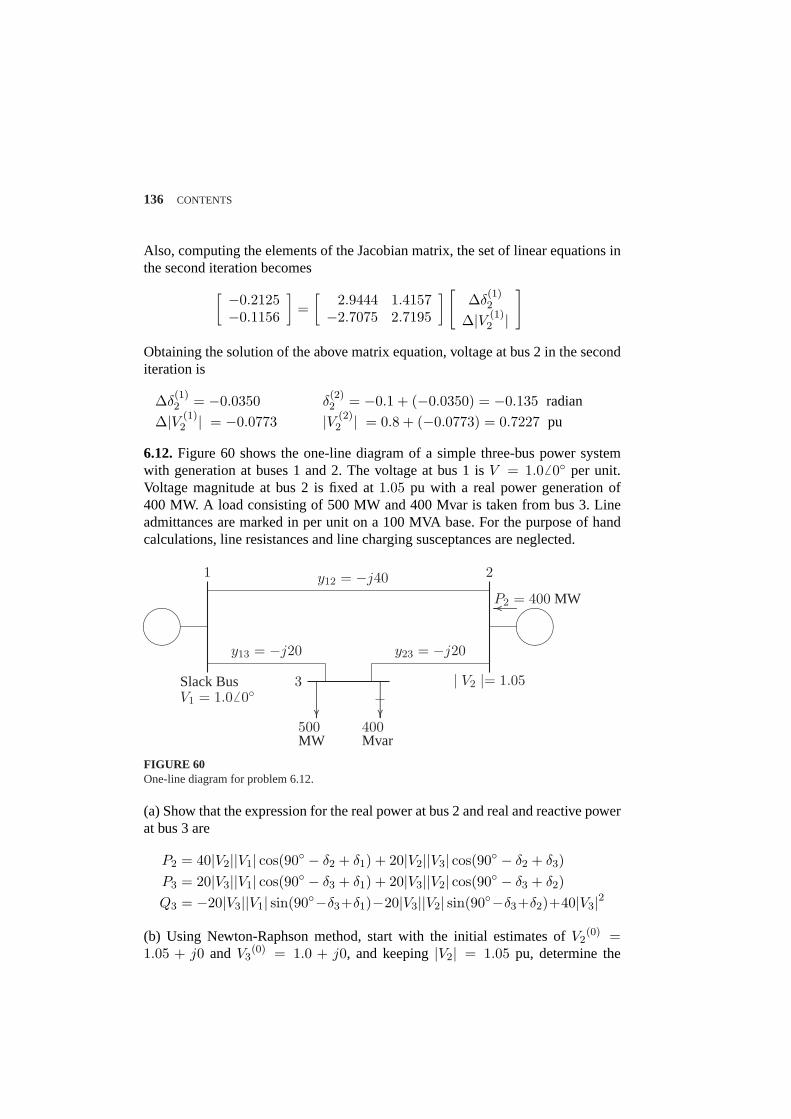
136 CONTENTS
Also, computing the elements of the Jacobian matrix, the set of linear equations inthe second iteration becomes
[ −0.2125−0.1156
]=
[2.9444 1.4157
−2.7075 2.7195
] [∆δ
(1)2
∆|V (1)2 |
]
Obtaining the solution of the above matrix equation, voltage at bus 2 in the seconditeration is
∆δ(1)2 = −0.0350 δ
(2)2 = −0.1 + (−0.0350) = −0.135 radian
∆|V (1)2 | = −0.0773 |V (2)
2 | = 0.8 + (−0.0773) = 0.7227 pu
6.12.Figure 60 shows the one-line diagram of a simple three-bus power systemwith generation at buses 1 and 2. The voltage at bus 1 isV = 1.0 6 0 per unit.Voltage magnitude at bus 2 is fixed at1.05 pu with a real power generation of400 MW. A load consisting of 500 MW and 400 Mvar is taken from bus 3. Lineadmittances are marked in per unit on a 100 MVA base. For the purpose of handcalculations, line resistances and line charging susceptances are neglected.
½¼
¾»
.............................................................................
........
........
........
.............................................................................
........
........
........
½¼
¾»...........................................................................
y12 = −j40
y13 = −j20 y23 = −j20
V1 = 1.06 0| V2 |= 1.05Slack Bus
500MW
400Mvar
P2 = 400 MW
1 2
3
FIGURE 60One-line diagram for problem 6.12.
(a) Show that the expression for the real power at bus 2 and real and reactive powerat bus 3 are
P2 = 40|V2||V1| cos(90 − δ2 + δ1) + 20|V2||V3| cos(90 − δ2 + δ3)P3 = 20|V3||V1| cos(90 − δ3 + δ1) + 20|V3||V2| cos(90 − δ3 + δ2)Q3 = −20|V3||V1| sin(90−δ3+δ1)−20|V3||V2| sin(90−δ3+δ2)+40|V3|2
(b) Using Newton-Raphson method, start with the initial estimates ofV2(0) =
1.05 + j0 and V3(0) = 1.0 + j0, and keeping|V2| = 1.05 pu, determine the
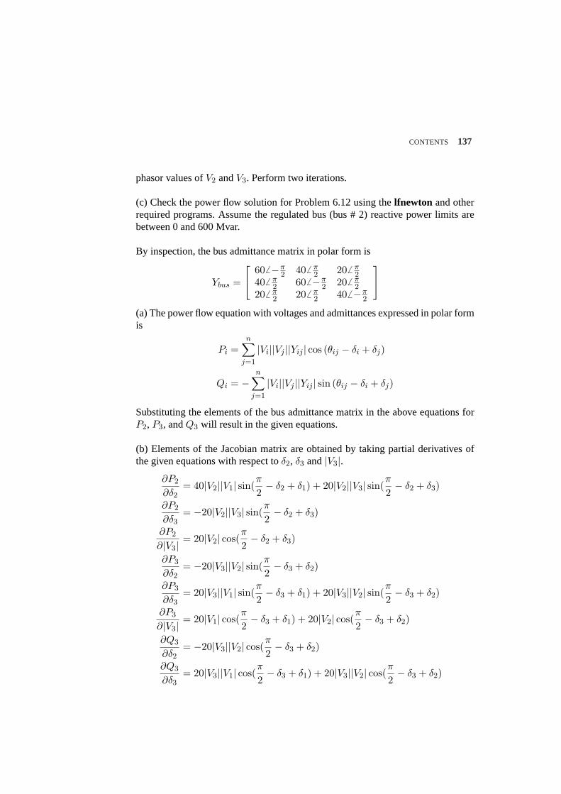
CONTENTS 137
phasor values ofV2 andV3. Perform two iterations.
(c) Check the power flow solution for Problem 6.12 using thelfnewton and otherrequired programs. Assume the regulated bus (bus # 2) reactive power limits arebetween 0 and 600 Mvar.
By inspection, the bus admittance matrix in polar form is
Ybus =
606 −π2 406 π
2 206 π2
406 π2 606 −π
2 206 π2
206 π2 206 π
2 406 −π2
(a) The power flow equation with voltages and admittances expressed in polar formis
Pi =n∑
j=1
|Vi||Vj ||Yij | cos (θij − δi + δj)
Qi = −n∑
j=1
|Vi||Vj ||Yij | sin (θij − δi + δj)
Substituting the elements of the bus admittance matrix in the above equations forP2, P3, andQ3 will result in the given equations.
(b) Elements of the Jacobian matrix are obtained by taking partial derivatives ofthe given equations with respect toδ2, δ3 and|V3|.
∂P2
∂δ2= 40|V2||V1| sin(
π
2− δ2 + δ1) + 20|V2||V3| sin(
π
2− δ2 + δ3)
∂P2
∂δ3= −20|V2||V3| sin(
π
2− δ2 + δ3)
∂P2
∂|V3| = 20|V2| cos(π
2− δ2 + δ3)
∂P3
∂δ2= −20|V3||V2| sin(
π
2− δ3 + δ2)
∂P3
∂δ3= 20|V3||V1| sin(
π
2− δ3 + δ1) + 20|V3||V2| sin(
π
2− δ3 + δ2)
∂P3
∂|V3| = 20|V1| cos(π
2− δ3 + δ1) + 20|V2| cos(
π
2− δ3 + δ2)
∂Q3
∂δ2= −20|V3||V2| cos(
π
2− δ3 + δ2)
∂Q3
∂δ3= 20|V3||V1| cos(
π
2− δ3 + δ1) + 20|V3||V2| cos(
π
2− δ3 + δ2)
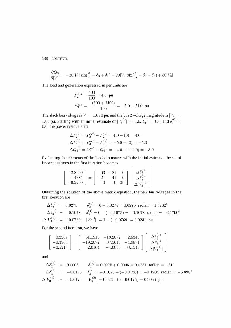
138 CONTENTS
∂Q3
∂|V3| = −20|V1| sin(π
2− δ3 + δ1)− 20|V2| sin(
π
2− δ3 + δ2) + 80|V3|
The load and generation expressed in per units are
P sch2 =
400100
= 4.0 pu
Ssch3 = −(500 + j400)
100= −5.0− j4.0 pu
The slack bus voltage isV1 = 1.0 6 0 pu, and the bus 2 voltage magnitude is|V2| =1.05 pu. Starting with an initial estimate of|V (0)
3 | = 1.0, δ(0)2 = 0.0, andδ
(0)3 =
0.0, the power residuals are
∆P(0)2 = P sch
2 − P(0)2 = 4.0− (0) = 4.0
∆P(0)3 = P sch
3 − P(0)3 = −5.0− (0) = −5.0
∆Q(0)3 = Qsch
3 −Q(0)3 = −4.0− (−1.0) = −3.0
Evaluating the elements of the Jacobian matrix with the initial estimate, the set oflinear equations in the first iteration becomes
−2.8600
1.4384−0.2200
=
63 −21 0−21 41 0
0 0 39
∆δ(0)2
∆δ(0)3
∆|V (0)3 |
Obtaining the solution of the above matrix equation, the new bus voltages in thefirst iteration are
∆δ(0)2 = 0.0275 δ
(1)2 = 0 + 0.0275 = 0.0275 radian= 1.5782
∆δ(0)3 = −0.1078 δ
(1)3 = 0 + (−0.1078) = −0.1078 radian= −6.1790
∆|V (0)3 | = −0.0769 |V (1)
3 | = 1 + (−0.0769) = 0.9231 pu
For the second iteration, we have
0.2269−0.3965−0.5213
=
61.1913 −19.2072 2.8345−19.2072 37.5615 −4.9871
2.6164 −4.6035 33.1545
∆δ(1)2
∆δ(1)3
∆|V (1)3 |
and
∆δ(1)2 = 0.0006 δ
(2)2 = 0.0275 + 0.0006 = 0.0281 radian= 1.61
∆δ(1)3 = −0.0126 δ
(2)3 = −0.1078 + (−0.0126) = −0.1204 radian= −6.898
∆|V (1)3 | = −0.0175 |V (2)
3 | = 0.9231 + (−0.0175) = 0.9056 pu
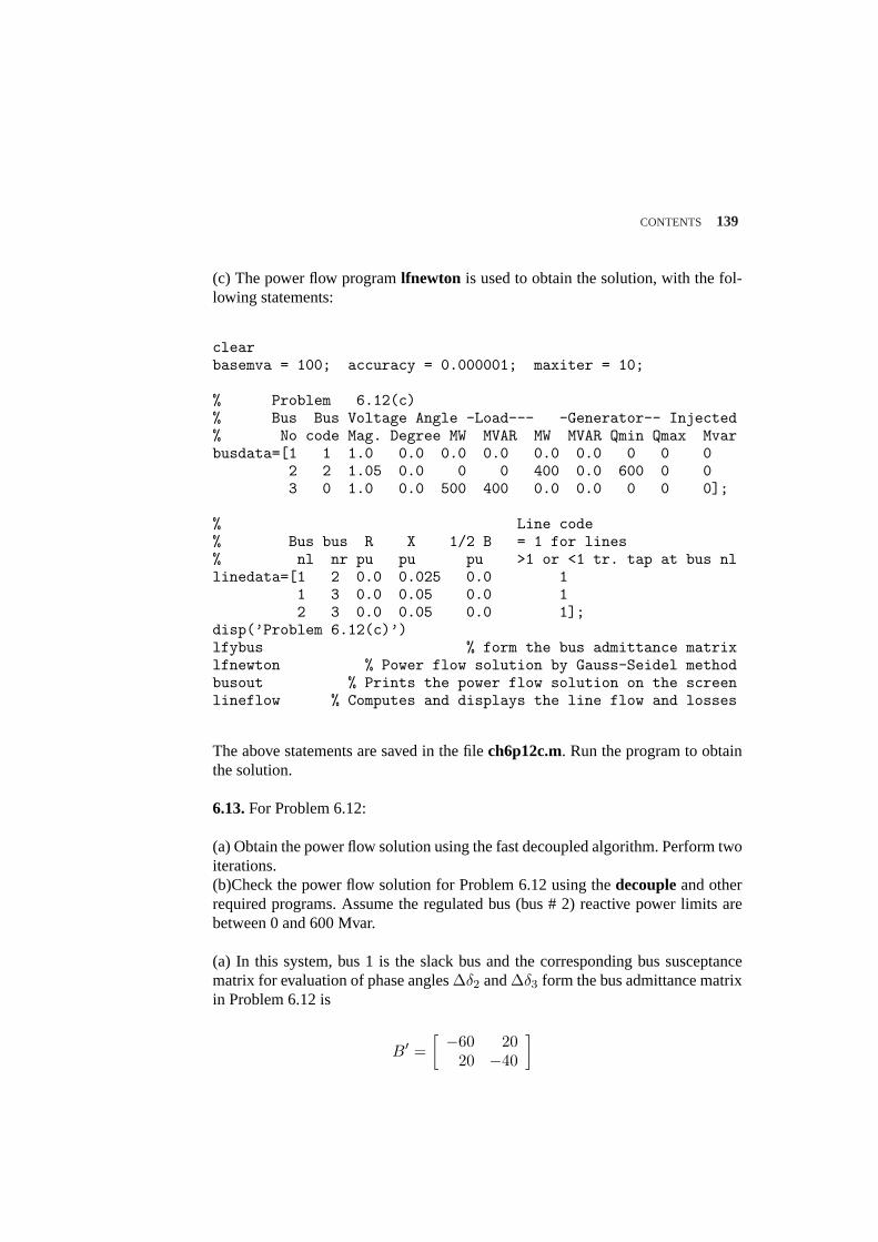
CONTENTS 139
(c) The power flow programlfnewton is used to obtain the solution, with the fol-lowing statements:
clearbasemva = 100; accuracy = 0.000001; maxiter = 10;
% Problem 6.12(c)% Bus Bus Voltage Angle -Load--- -Generator-- Injected% No code Mag. Degree MW MVAR MW MVAR Qmin Qmax Mvarbusdata=[1 1 1.0 0.0 0.0 0.0 0.0 0.0 0 0 0
2 2 1.05 0.0 0 0 400 0.0 600 0 03 0 1.0 0.0 500 400 0.0 0.0 0 0 0];
% Line code% Bus bus R X 1/2 B = 1 for lines% nl nr pu pu pu >1 or <1 tr. tap at bus nllinedata=[1 2 0.0 0.025 0.0 1
1 3 0.0 0.05 0.0 12 3 0.0 0.05 0.0 1];
disp(’Problem 6.12(c)’)lfybus % form the bus admittance matrixlfnewton % Power flow solution by Gauss-Seidel methodbusout % Prints the power flow solution on the screenlineflow % Computes and displays the line flow and losses
The above statements are saved in the filech6p12c.m. Run the program to obtainthe solution.
6.13.For Problem 6.12:
(a) Obtain the power flow solution using the fast decoupled algorithm. Perform twoiterations.(b)Check the power flow solution for Problem 6.12 using thedecoupleand otherrequired programs. Assume the regulated bus (bus # 2) reactive power limits arebetween 0 and 600 Mvar.
(a) In this system, bus 1 is the slack bus and the corresponding bus susceptancematrix for evaluation of phase angles∆δ2 and∆δ3 form the bus admittance matrixin Problem 6.12 is
B′ =[ −60 20
20 −40
]
140 CONTENTS
The inverse of the above matrix is
[B′]−1 =[ −0.02 −0.01−0.01 −0.03
]
The expressions for real power at bus 2 and 3 and the reactive power at bus 3 aregiven in Problem 6.12. The slack bus voltage isV1 = 1.0 6 0 pu, and the bus 2voltage magnitude is|V3| = 1.05 pu. Starting with an initial estimate of|V (0)
3 | =1.0, δ
(0)2 = 0.0, andδ
(0)3 = 0.0, the power residuals are computed from (6.63) and
(6.64)
∆P(0)2 = P sch
2 − P(0)2 = 4− (0) = 4
∆P(0)3 = P sch
3 − P(0)3 = −5− (0) = −5
∆Q(0)3 = Qsch
3 −Q(0)3 = −4− (−1) = −3
The fast decoupled power flow algorithm given by (6.77) becomes ∆δ
(0)2
∆δ(0)3
= −
[ −0.02 −0.0−0.01 −0.03
] [4
1.05−51.0
]=
[.0262
−0.1119
]
Since bus 2 is a regulated bus, the corresponding row and column ofB′ are elimi-nated and we get
B′′ = [−40]
From (6.78), we have
∆|V3| = −[−1
40
] [−31.0
]= −0.075
The new bus voltages in the first iteration are
∆δ(0)2 = 0.0262 δ
(1)2 = 0 + (0.0262) = 0.0262 radian= 1.5006
∆δ(0)3 = −0.1119 δ
(1)3 = 0 + (−0.1119) = −0.1119 radian= −6.4117
∆|V (0)3 | = −0.075 |V (1)
2 | = 1 + (−0.075) = 0.925 pu
For the second iteration, the power residuals are
∆P(1)2 = P sch
2 − P(1)2 = 4− (3.7739) = 0.2261
∆P(1)3 = P sch
3 − P(1)3 = −5− (−4.7399) = −.2601
∆Q(1)3 = Qsch
3 −Q(1)3 = −4− (−3.3994) = −0.6006
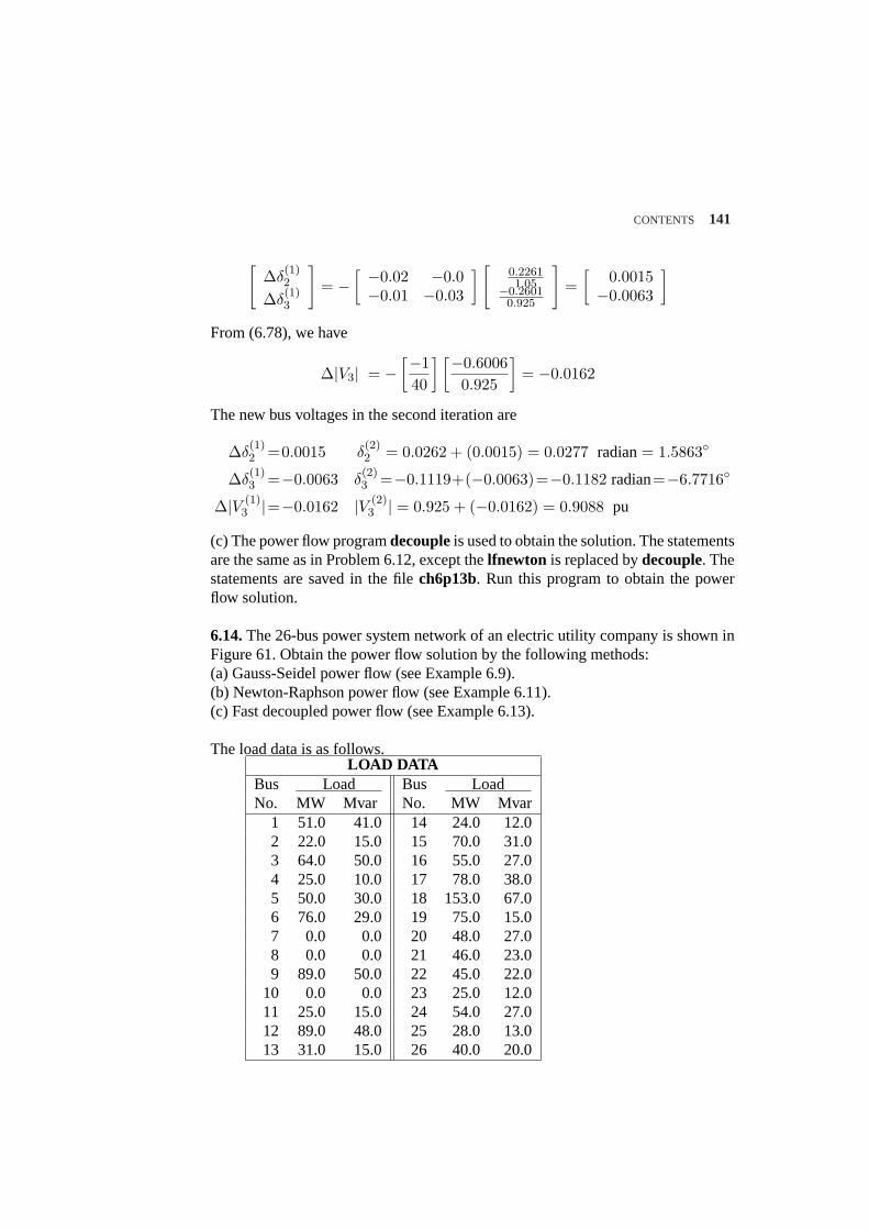
CONTENTS 141
[∆δ
(1)2
∆δ(1)3
]= −
[ −0.02 −0.0−0.01 −0.03
] [0.22611.05−0.2601
0.925
]=
[0.0015
−0.0063
]
From (6.78), we have
∆|V3| = −[−1
40
] [−0.60060.925
]= −0.0162
The new bus voltages in the second iteration are
∆δ(1)2 =0.0015 δ
(2)2 = 0.0262 + (0.0015) = 0.0277 radian= 1.5863
∆δ(1)3 =−0.0063 δ
(2)3 =−0.1119+(−0.0063)=−0.1182 radian=−6.7716
∆|V (1)3 |=−0.0162 |V (2)
3 | = 0.925 + (−0.0162) = 0.9088 pu
(c) The power flow programdecoupleis used to obtain the solution. The statementsare the same as in Problem 6.12, except thelfnewton is replaced bydecouple. Thestatements are saved in the filech6p13b. Run this program to obtain the powerflow solution.
6.14.The 26-bus power system network of an electric utility company is shown inFigure 61. Obtain the power flow solution by the following methods:(a) Gauss-Seidel power flow (see Example 6.9).(b) Newton-Raphson power flow (see Example 6.11).(c) Fast decoupled power flow (see Example 6.13).
The load data is as follows.LOAD DATA
Bus Load Bus LoadNo. MW Mvar No. MW Mvar
1 51.0 41.0 14 24.0 12.02 22.0 15.0 15 70.0 31.03 64.0 50.0 16 55.0 27.04 25.0 10.0 17 78.0 38.05 50.0 30.0 18 153.0 67.06 76.0 29.0 19 75.0 15.07 0.0 0.0 20 48.0 27.08 0.0 0.0 21 46.0 23.09 89.0 50.0 22 45.0 22.0
10 0.0 0.0 23 25.0 12.011 25.0 15.0 24 54.0 27.012 89.0 48.0 25 28.0 13.013 31.0 15.0 26 40.0 20.0
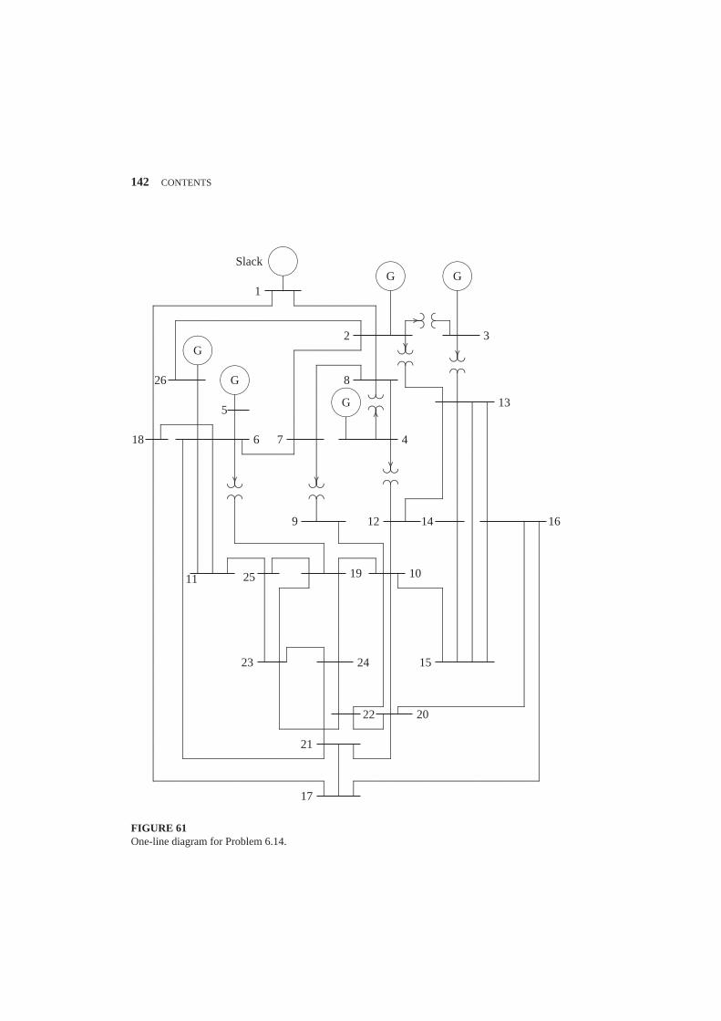
142 CONTENTS
........
........
........
..........................................................................................................................................................................................................................................................................................................................................................................................................................................................................................................................................................................................................................................................................................................................................................................................................................................................................................................................................................................................................................................................................................................................................................................................................................................................................................................................................................................................................................................................................................................................................................................................................................................................
........
........
........
...
........
........
........
.................................................................................................................................................................................................................................................................................................................................................................................................................................................................................................................................................................................................................................................................................................................................................................................................................................................................................................................................................................................................................................................................................................................................................................................................................................................................................................................... ...................................................................................................................................................
........
........
........
........
........
........
........
........
........
........
........
........
........
........
........
........
........
........
........
........
........
........
........
........
........
............................................................................................................................................................................................................................................................................................................................................................................................................................................................................................................................................................................................................................................................................................................................................
........
........
........
.......................................................................................................................................................................................................................................................................................................................................................................................................................................
...............................................................................................................................................................................................................................................................................................................................................................................................................................................
.................................................................................................................................................................................................
........
........
........
........................................................................................................................................................................................................................................................................................................................................................................................................................................................................................................................................................................................................................................................................................
........
........
........
.............................................................................................................................................................................................................................................................................................................................................................................................................................................................................................................................................................................................................................................................................................................................................................................................................................................................................................................................................................................................................................................................................................................................
............................................................................................................................
..............................................................................................................................................................................................................................................................
........
........
........
............................................... ........................................................................................................................................................................................................................................................................................................................................................................................................................................................................................................................................................................................................................................................................................................
........
........
........
........
........
.......
.................................................................................................................................................................................................................................................................................................................................................................................................
........
........
........
........
........
........
........
......................
................
.................................................................................................................................................................................................
........
........
........
.....................................................................................................................................................................................................................................................................................................................................................................................................................................................................................................................................................................................................................................................................................................
............................................... ................ ..............................................................
......................................................................
........
........
........
.............................................................................................
........
........
........
........
........
............................................................................................................................................................................................................................................................................................................................................................................................................
........
........
........
........
........
...
...................................................................................................................................................................................................................................................................................... .......................................................................................................................................................................................................................................................................................................................................................................................................................................................................................................................................................................................................................
...................................................................................................................................................
........
........
........
........
........
........
........
........
........
........
........
........
........
........
........
........
........
........
........
........
........
........
........
........
........
........
........
........
........
........
........
........
........
........
........
........
........
........
........
........
........
........
........
........
........
........
........
........
........
........
........
........
........
........
........
........
........
........
........
........
........
........
........
........
........
........
........
........
........
........
..
........
........
........
........
........
........
........
........
........
........
........
........
........
........
........
........
........
........
........
........
........
........
........
........
........
........
........
........
........
........
........
........
........
........
........
........
........
........
........
........
........
........
........
........
........
........
........
........
........
........
........
........
........
........
........
........
........
........
........
........
........
........
........
........
........
........
........
..
........
..............................................................................................................................................................................................................................................................................................................................................................................................................................................................................................................................................................................................................................................................................
........
........
........
.................................................................................................................................................................................................................................................................................................................................................................................................................................................................................................................................................................................................................................................................................................................................................................................................................................................................................................................................................................
........
........
........
........
........
........
........
........
........
........
........
........
........
....
........
........
........
.......¹¸
º·
¹¸
º·
¹¸
º·
¹¸
º·
¹¸
º·
¹¸
º·
..................................................
....................................
.......................................
.........................
....................................
..............
..................................................
....................................
..............
..................................................
....................................
..............
..................................................
....................................
..............
..................................................
....................................
..............
..................................................
..................................................
1
2 3
26
5
8
13
18 6 7 4
9 12 14 16
11 25 19 10
23 24 15
22 20
21
17
G G
G
G
G
Slack
FIGURE 61One-line diagram for Problem 6.14.
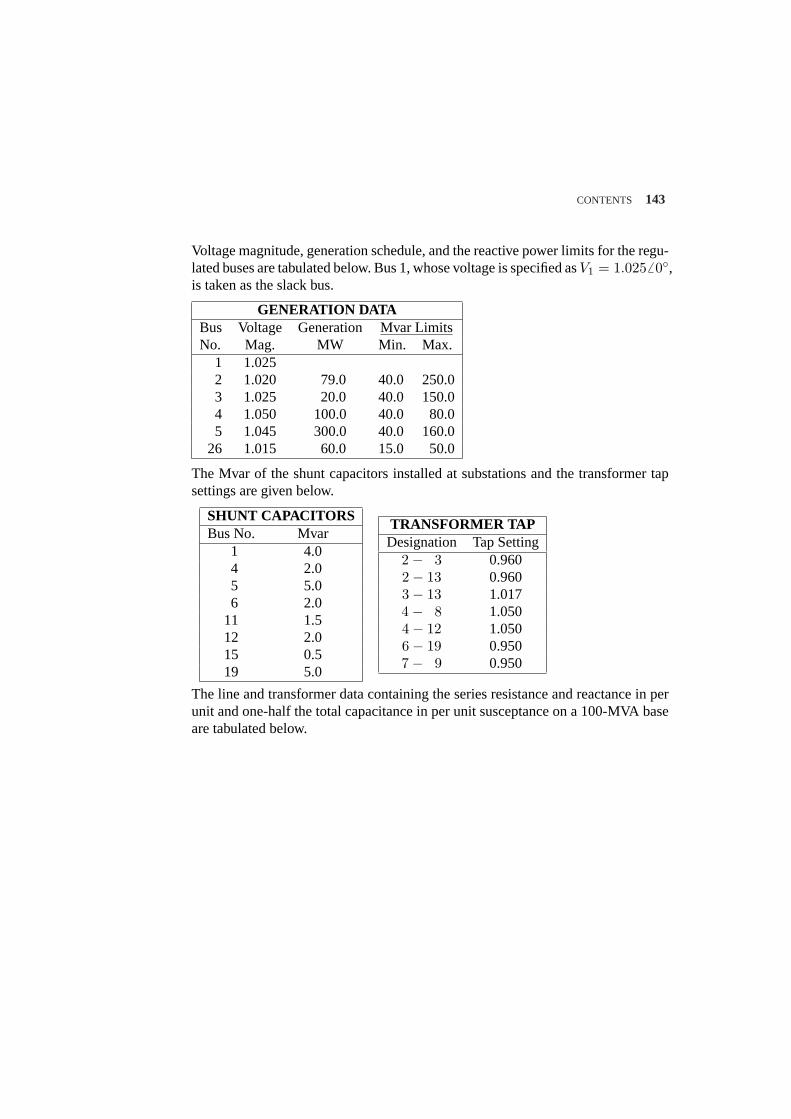
CONTENTS 143
Voltage magnitude, generation schedule, and the reactive power limits for the regu-lated buses are tabulated below. Bus 1, whose voltage is specified asV1 = 1.0256 0,is taken as the slack bus.
GENERATION DATABus Voltage Generation Mvar LimitsNo. Mag. MW Min. Max.
1 1.0252 1.020 79.0 40.0 250.03 1.025 20.0 40.0 150.04 1.050 100.0 40.0 80.05 1.045 300.0 40.0 160.0
26 1.015 60.0 15.0 50.0
The Mvar of the shunt capacitors installed at substations and the transformer tapsettings are given below.
SHUNT CAPACITORSBus No. Mvar
1 4.04 2.05 5.06 2.0
11 1.512 2.015 0.519 5.0
TRANSFORMER TAPDesignation Tap Setting
2− 3 0.9602− 13 0.9603− 13 1.0174− 8 1.0504− 12 1.0506− 19 0.9507− 9 0.950
The line and transformer data containing the series resistance and reactance in perunit and one-half the total capacitance in per unit susceptance on a 100-MVA baseare tabulated below.
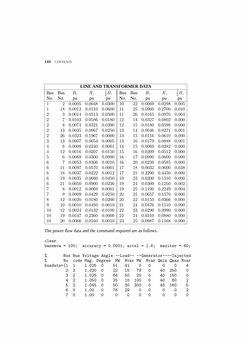
144 CONTENTS
LINE AND TRANSFORMER DATABus Bus R, X, 1
2B, Bus Bus R, X, 12B,
No. No. pu pu pu No. No. pu pu pu1 2 0.0005 0.0048 0.0300 10 22 0.0069 0.0298 0.0051 18 0.0013 0.0110 0.0600 11 25 0.0960 0.2700 0.0102 3 0.0014 0.0513 0.0500 11 26 0.0165 0.0970 0.0042 7 0.0103 0.0586 0.0180 12 14 0.0327 0.0802 0.0002 8 0.0074 0.0321 0.0390 12 15 0.0180 0.0598 0.0002 13 0.0035 0.0967 0.0250 13 14 0.0046 0.0271 0.0012 26 0.0323 0.1967 0.0000 13 15 0.0116 0.0610 0.0003 13 0.0007 0.0054 0.0005 13 16 0.0179 0.0888 0.0014 8 0.0008 0.0240 0.0001 14 15 0.0069 0.0382 0.0004 12 0.0016 0.0207 0.0150 15 16 0.0209 0.0512 0.0005 6 0.0069 0.0300 0.0990 16 17 0.0990 0.0600 0.0006 7 0.0053 0.0306 0.0010 16 20 0.0239 0.0585 0.0006 11 0.0097 0.0570 0.0001 17 18 0.0032 0.0600 0.0386 18 0.0037 0.0222 0.0012 17 21 0.2290 0.4450 0.0006 19 0.0035 0.0660 0.0450 19 23 0.0300 0.1310 0.0006 21 0.0050 0.0900 0.0226 19 24 0.0300 0.1250 0.0027 8 0.0012 0.0069 0.0001 19 25 0.1190 0.2249 0.0047 9 0.0009 0.0429 0.0250 20 21 0.0657 0.1570 0.0008 12 0.0020 0.0180 0.0200 20 22 0.0150 0.0366 0.0009 10 0.0010 0.0493 0.0010 21 24 0.0476 0.1510 0.00010 12 0.0024 0.0132 0.0100 22 23 0.0290 0.0990 0.00010 19 0.0547 0.2360 0.0000 22 24 0.0310 0.0880 0.00010 20 0.0066 0.0160 0.0010 23 25 0.0987 0.1168 0.000
The power flow data and the command required are as follows.
clearbasemva = 100; accuracy = 0.0001; accel = 1.6; maxiter = 60;
% Bus Bus Voltage Angle --Load-- --Generator----Injected% No code Mag. Degree MW Mvar MW Mvar Qmin Qmax Mvarbusdata=[1 1 1.025 0 51 41 0 0 0 0 4
2 2 1.020 0 22 15 79 0 40 250 03 2 1.025 0 64 50 20 0 40 150 04 2 1.050 0 25 10 100 0 40 80 25 2 1.045 0 50 30 300 0 40 160 56 0 1.00 0 76 29 0 0 0 0 27 0 1.00 0 0 0 0 0 0 0 0
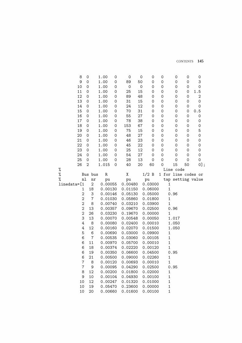
CONTENTS 145
8 0 1.00 0 0 0 0 0 0 0 09 0 1.00 0 89 50 0 0 0 0 310 0 1.00 0 0 0 0 0 0 0 011 0 1.00 0 25 15 0 0 0 0 1.512 0 1.00 0 89 48 0 0 0 0 213 0 1.00 0 31 15 0 0 0 0 014 0 1.00 0 24 12 0 0 0 0 015 0 1.00 0 70 31 0 0 0 0 0.516 0 1.00 0 55 27 0 0 0 0 017 0 1.00 0 78 38 0 0 0 0 018 0 1.00 0 153 67 0 0 0 0 019 0 1.00 0 75 15 0 0 0 0 520 0 1.00 0 48 27 0 0 0 0 021 0 1.00 0 46 23 0 0 0 0 022 0 1.00 0 45 22 0 0 0 0 023 0 1.00 0 25 12 0 0 0 0 024 0 1.00 0 54 27 0 0 0 0 025 0 1.00 0 28 13 0 0 0 0 026 2 1.015 0 40 20 60 0 15 50 0];
% Line code% Bus bus R X 1/2 B 1 for line codes or% nl nr pu pu pu tap setting valuelinedata=[1 2 0.00055 0.00480 0.03000 1
1 18 0.00130 0.01150 0.06000 12 3 0.00146 0.05130 0.05000 0.962 7 0.01030 0.05860 0.01800 12 8 0.00740 0.03210 0.03900 12 13 0.00357 0.09670 0.02500 0.962 26 0.03230 0.19670 0.00000 13 13 0.00070 0.00548 0.00050 1.0174 8 0.00080 0.02400 0.00010 1.0504 12 0.00160 0.02070 0.01500 1.0505 6 0.00690 0.03000 0.09900 16 7 0.00535 0.03060 0.00105 16 11 0.00970 0.05700 0.00010 16 18 0.00374 0.02220 0.00120 16 19 0.00350 0.06600 0.04500 0.956 21 0.00500 0.09000 0.02260 17 8 0.00120 0.00693 0.00010 17 9 0.00095 0.04290 0.02500 0.958 12 0.00200 0.01800 0.02000 19 10 0.00104 0.04930 0.00100 1
10 12 0.00247 0.01320 0.01000 110 19 0.05470 0.23600 0.00000 110 20 0.00660 0.01600 0.00100 1
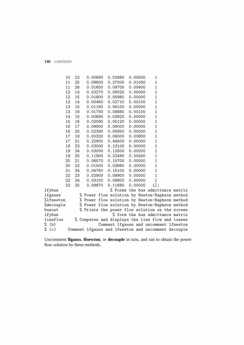
146 CONTENTS
10 22 0.00690 0.02980 0.00500 111 25 0.09600 0.27000 0.01000 111 26 0.01650 0.09700 0.00400 112 14 0.03270 0.08020 0.00000 112 15 0.01800 0.05980 0.00000 113 14 0.00460 0.02710 0.00100 113 15 0.01160 0.06100 0.00000 113 16 0.01793 0.08880 0.00100 114 15 0.00690 0.03820 0.00000 115 16 0.02090 0.05120 0.00000 116 17 0.09900 0.06000 0.00000 116 20 0.02390 0.05850 0.00000 117 18 0.00320 0.06000 0.03800 117 21 0.22900 0.44500 0.00000 119 23 0.03000 0.13100 0.00000 119 24 0.03000 0.12500 0.00200 119 25 0.11900 0.22490 0.00400 120 21 0.06570 0.15700 0.00000 120 22 0.01500 0.03660 0.00000 121 24 0.04760 0.15100 0.00000 122 23 0.02900 0.09900 0.00000 122 24 0.03100 0.08800 0.00000 123 25 0.09870 0.11680 0.00000 1];
lfybus % Forms the bus admittance matrixlfgauss % Power flow solution by Newton-Raphson method%lfnewton % Power flow solution by Newton-Raphson method%decouple % Power flow solution by Newton-Raphson methodbusout % Prints the power flow solution on the screenlfybus % form the bus admittance matrixlineflow % Computes and displays the line flow and losses% (b) Comment lfgauss and uncomment lfnewton% (c) Comment lfgauss and lfnewton and uncomment decouple
Uncommentlfgauss, lfnewton, or decouplein turn, and run to obtain the powerflow solution by these methods.
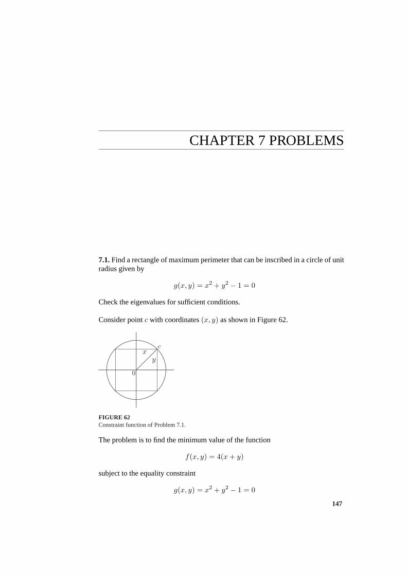
CHAPTER 7 PROBLEMS
7.1.Find a rectangle of maximum perimeter that can be inscribed in a circle of unitradius given by
g(x, y) = x2 + y2 − 1 = 0
Check the eigenvalues for sufficient conditions.
Consider pointc with coordinates(x, y) as shown in Figure 62.
.................................................................................................................................................
..................................................................................................................................................................................................
.........................
.........................................
......................................................................................................................................................................................................................................................................................
.....................................................................................................................................................................................................................................................................................
........
........
........
........
........
........
........
........
........
........
........
........
........
........
........
........
........
........
........
........
........
........
........
........
........
........
........
........
........
........
........
........
........
........
.....
xy
.............................................................................................................
0
c
FIGURE 62Constraint function of Problem 7.1.
The problem is to find the minimum value of the function
f(x, y) = 4(x + y)
subject to the equality constraint
g(x, y) = x2 + y2 − 1 = 0
147
148 CONTENTS
Forming the Lagrangian function, we obtain
L = 4(x + y) + λ(x2 + y2 − 1)
The resulting necessary conditions for constrained local maxima ofL are
∂L∂x
= 4 + 2λx = 0
∂L∂y
= 4 + 2λy = 0
∂L∂λ
= x2 + y2 − 1 = 0
From the first two conditions, we obtainx = y. Substituting fory in the thirdcondition results in
2x2 = 1
or
x = y = 0.707 and λ = − 42(0.707)
= −2.828
and the perimeter is
p = 4(x + y) = 4(0.707 + 0.707) = 5.656
To see if the perimeter is a maximum, we evaluate the second derivatives and formthe Hessian matrix
H =[
2λ 00 2λ
]=
[ −5.656 00 −5.656
]
The second partial derivatives are negative, thusp is a maximum.
7.2.Find the minimum of the function
f(x, y) = x2 + 2y2
subject to the equality constraint
g(x, y) = x + 2y + 4 = 0
Check for the sufficient conditions.
CONTENTS 149
Forming the Lagrangian function, we obtain
L = x2 + 2y2 + λ(x + 2y + 4)
The resulting necessary conditions for constrained local minima ofL are
∂L∂x
= 2x + λ = 0
∂L∂y
= 4y + 2λ = 0
∂L∂λ
= x + 2y + 4 = 0
From the first two conditions, we obtainx = y. Substituting fory in the thirdcondition results in
3x = −4
or
x = y = −43
and λ = −2x =83
and the minimum distance is
f(x, y) = x2 + 2y2 =(−4
3
)2
+ 2(−4
3
)2
= 5.333
To see if this distance is a minimum, we evaluate the second derivatives and formthe Hessian matrix
H =[
2 00 4
]
The second partial derivatives are positive, thus the minimum distance to origin isat point(x, y) = (−4
3 ,−43).
7.3.Use the Lagrangian multiplier method for solving constrained parameter op-timization problems to determine an isosceles triangle of maximum area that maybe inscribed in a circle of radius1.
Consider pointc with coordinates(x, 1 + y) as shown in Figure 63. The problemis to maximize the area of the triangle given by
f(x, y) = x(1 + y)
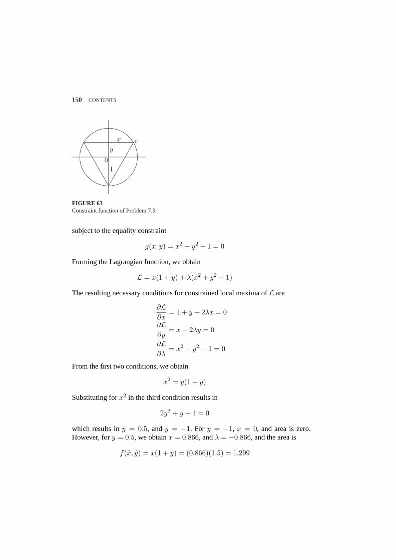
150 CONTENTS
.................................................................................................................................................
..................................................................................................................................................................................................
.........................
.........................................
......................................................................................................................................................................................................................................................................................
.........................................................................................................................................................................................................................................................................................................................................................................................................................................................................................................................................................................................
.....................................................................................................................................................................................................................................................................................
........
........
........
........
........
........
........
........
........
........
........
........
........
........
........
........
........
........
........
........
........
........
........
........
........
........
........
........
........
........
........
........
........
........
.....
x
y
10
c
FIGURE 63Constraint function of Problem 7.3.
subject to the equality constraint
g(x, y) = x2 + y2 − 1 = 0
Forming the Lagrangian function, we obtain
L = x(1 + y) + λ(x2 + y2 − 1)
The resulting necessary conditions for constrained local maxima ofL are
∂L∂x
= 1 + y + 2λx = 0
∂L∂y
= x + 2λy = 0
∂L∂λ
= x2 + y2 − 1 = 0
From the first two conditions, we obtain
x2 = y(1 + y)
Substituting forx2 in the third condition results in
2y2 + y − 1 = 0
which results iny = 0.5, andy = −1. For y = −1, x = 0, and area is zero.However, fory = 0.5, we obtainx = 0.866, andλ = −0.866, and the area is
f(x, y) = x(1 + y) = (0.866)(1.5) = 1.299
CONTENTS 151
7.4.For a second-order bandpass filter with transfer function
H(s) =ω2
n
s2 + 2ζωns + ω2n
determine the values of the damping ratio and natural frequency,ζ andωn, cor-responding to a Bode plot whose peak occurs at 7071.07 radians/sec and whosehalf-power bandwidth is 12,720.2 radians/sec.
The frequency response transfer function is
H(jω) =ω2
n
−ω2n + j2ζωnω + ω2
n
or
H(jω) =1
1−(
ωωn
)2+ j2ζ
(ωωn
)
The magnitude of the frequency response transfer function is
|H(jω)| = 1[(
1−(
ωωn
)2)2
+ 4ζ2(
ωωn
)2]1/2
The amplitude is maximum when the denominator is minimum. Thus the problemis to minimize the function
f(ω) =
(1−
(ω
ωn
)2)2
+ 4ζ2(
ω
ωn
)2
|H(jω)| is maximum whendf(ω)dω = 0. This condition results in the peak resonant
frequency given by
ωr = ωn
√1− 2ζ2 (P7.1)
At the one-half power frequencyωB, we have
1(1−
(ωBωn
)2)2
+ 4ζ2(
ωBωn
)2=
12
Solving for(
ωBωn
)2results in
(ωB
ωn
)2
=(1− 2ζ2
)±
√(1− 2ζ2)2 + 1 (P7.2)
152 CONTENTS
From (P7.1), we have
(1− 2ζ2
)=
(ωr
ωn
)2
(P7.3)
Substituting from (P7.3) into (P7.2), and considering the positive term, results in
(ωB
ωn
)2
=(
ωr
ωn
)2
+
√(ωr
ωn
)4
+ 1
From the above expression, we obtain
ω4n = ω2
B
(ω2
B − 2ω2r
)(P7.4)
Substituting forωr = 7, 071.07 rad/s, andωB = 12, 720.2 rad/s, results inωn =10, 000 rad/s, and from (P7.3), we have
(1− 2ζ2
)=
(7, 071.0710, 000
)2
or
ζ = 0.5
7.5.Find the minimum value of the function
f(x, y) = x2 + y2
subject to the equality constraint
g(x, y) = x2 − 6x− y2 + 17 = 0
Forming the Lagrangian function, we obtain
L = x2 + y2 + λ(x2 − 6x− y2 + 17)
The resulting necessary conditions for constrained local maxima ofL are
∂L∂x
= 2x + λ(2x− 6) = 0
∂L∂y
= 2y − 2λy = 0
∂L∂λ
= x2 − 6x− y2 + 17 = 0
CONTENTS 153
From the second conditionλ = 1. Substituting in the first condition
2x + (1)(2x− 6) = 0 or x = 1.5
Substituting forx in the third condition results iny = 3.20156. Thus the minimumvalue of the function is
f(x, y) = (1.5)2 + (3.20156)2 = 12.5
7.6.Find the minimum value of the function
f(x, y) = x2 + y2
subject to one equality constraint
g(x, y) = x2 − 5x− y2 + 20 = 0
and one inequality constraint
u(x, y) = 2x + y ≥ 6
The unconstrained cost function from (7.16) is
L = x2 + y2 + λ(x2 − 5x− y2 + 20) + µ(2x + y − 6)
The resulting necessary conditions for constrained local minima ofL are
∂L∂x
= 2x + λ(2x− 5) + 2µ = 0
∂L∂y
= 2y − 2λy + µ = 0
∂L∂λ
= x2 − 5x− y2 + 20 = 0
∂L∂µ
= 2x + y − 6 = 0
Eliminatingµ from the first two equations result in
2x(λ + 1) + 4y(λ− 1) = 5λ
154 CONTENTS
From the fourth condition, we have
y = 6− 2x
Substituting fory in the above equation, yields
x =24− 19λ
10− 6λ
Now substituting forx in the previous equation, we get
y =12 + 2λ
10− 6λ
Substituting forx andy in the third condition (equality constraint) results in anequation in terms ofλ
(24− 19λ
10− 6λ
)2
− 5(
24− 19λ10− 6λ
)−
(12 + 2λ
10− 6λ
)2
+ 20 = 0
from which we have the following equation
507λ2 − 1690λ + 1232 = 0
Roots of the above equation areλ = 8839 andλ = 14
13 . Substituting for these valuesof λ in the expression forx andy, the corresponding extrema are
(x, y) = (163
,−143
) for λ =8839
, µ = −11.73
(x, y) = (1, 4) for λ =1413
, µ =813
The minimum distance from the cost function is17, located at point(1, 4), and themaximum distance is50.22 located at point(5.333,−4.666).
7.7.The fuel-cost functions in $/h for two 800 MW thermal plants are given by
C1 = 400 + 6.0P1 + 0.004P 21
C2 = 500 + βP2 + γP 22
whereP1 andP2 are in MW.
(a) The incremental cost of powerλ is $8/MWh when the total power demand is550 MW. Neglecting losses, determine the optimal generation of each plant.
CONTENTS 155
(b) The incremental cost of powerλ is $10/MWh when the total power demand is1300 MW. Neglecting losses, determine the optimal generation of each plant.(c) From the results of (a) and (b) find the fuel-cost coefficientsβ andγ of thesecond plant.
dC1
dP1= 6 + 0.008P1 = λ
dC2
dP2= β + 2γP2 = λ
(a) Forλ = 8, andPD = 550 MW, we have
P1 =8− 60.008
= 250 MW
P2 = PD − P1 = 500− 250 = 300 MW
(b) Forλ = 10, andPD = 1300 MW, we have
P1 =10− 60.008
= 500 MW
P2 = PD − P1 = 1300− 500 = 800 MW
(c) The incremental cost of power for plant 2 are given by
β + 2γ(300) = 8β + 2γ(800) = 10
Solving the above equations, we findβ = 6.8, andγ = 0.002
7.8.The fuel-cost functions in $/h for three thermal plants are given by
C1 = 350 + 7.20P1 + 0.0040P 21
C2 = 500 + 7.30P2 + 0.0025P 22
C3 = 600 + 6.74P3 + 0.0030P 23
whereP1, P2, andP3 are in MW. The governors are set such that generators sharethe load equally. Neglecting line losses and generator limits, find the total cost in$/h when the total load is
(i) PD = 450 MW(ii) PD = 745 MW(iii) PD = 1335 MW
156 CONTENTS
(i) For PD = 450 MW, P1 = P2 = P3 = 4503 = 150 MW. The total fuel cost is
Ct = 350 + 7.20(150) + 0.004(150)2 + 500 + 7.3(150) + 0.0025(150)2 +600 + 6.74(150) + 0.003(150)2 = 4, 849.75 $/h
(ii) For PD = 745 MW, P1 = P2 = P3 = 7453 MW. The total fuel cost is
Ct = 350 + 7.20(
7453
)+ 0.004
(7453
)2
+ 500 + 7.3(
7453
)+ 0.0025
(7453
)2
+600 + 6.74(
7453
)+ 0.003
(7453
)2
= 7, 310.46 $/h
(iii) For PD = 1335 MW, P1 = P2 = P3 = 445 MW. The total fuel cost is
Ct = 350 + 7.20(445) + 0.004(445)2 + 500 + 7.3(445) + 0.0025(445)2 +600 + 6.74(445) + 0.003(445)2 = 12, 783.04 $/h
7.9 Neglecting line losses and generator limits, determine the optimal schedulingof generation for each loading condition in Problem 7.8(a) by analytical technique, using (7.33) and (7.31).(b) using Iterative method. Start with an initial estimate ofλ = 7.5 $/MWh.(c) find the savings in $/h for each case compared to the costs in Problem 7.8 whenthe generators shared load equally.Use thedispatchprogram to check your results.
(a) (i) ForPD = 450 MW, from (7.33),λ is found to be
λ =450 + 7.2
0.008 + 7.30.005 + 6.74
0.0061
0.008 + 10.005 + 1
0.006
=450 + 3483.333
491.666= 8.0 $/MWh
Substituting forλ in the coordination equation, given by (7.31), the optimal dis-patch is
P1 =8.0− 7.22(0.004)
= 100
P2 =8.0− 7.32(0.0025)
= 140
P3 =8.0− 6.742(0.003)
= 210
CONTENTS 157
(a) (ii) ForPD = 745 MW, from (7.33),λ is found to be
λ =745 + 3483.333
491.666= 8.6 $/MWh
Substituting forλ in the coordination equation, given by (7.31), the optimal dis-patch is
P1 =8.6− 7.22(0.004)
= 175
P2 =8.6− 7.32(0.0025)
= 260
P3 =8.6− 6.742(0.003)
= 310
(a) (iii) For PD = 1335 MW, from (7.33),λ is found to be
λ =1335 + 3483.333
491.666= 9.8 $/MWh
Substituting forλ in the coordination equation, given by (7.31), the optimal dis-patch is
P1 =9.8− 7.22(0.004)
= 325
P2 =9.8− 7.32(0.0025)
= 500
P3 =9.8− 6.742(0.003)
= 510
(b) For the numerical solution using the gradient method, assume the initial valueof λ(1) = 7.5. From coordination equations, given by (7.31),P1, P2, andP3 are
P(1)1 =
7.5− 7.22(0.004)
= 37.5000
P(1)2 =
7.5− 7.32(0.0025)
= 40.0000
P(1)3 =
7.5− 6.742(0.003)
= 126.6666
(i) PD = 450 MW, the error∆P from (7.39) is
∆P (1) = 450− (37.5 + 40 + 126.6666) = 245.8333
158 CONTENTS
From (7.37)
∆λ(1) =245.8333491.6666
= 0.5
Therefore, the new value ofλ is
λ(2) = 7.5 + 0.5 = 8.0
Continuing the process, for the second iteration, we have
P(2)1 =
8.0− 7.22(0.004)
= 100
P(2)2 =
8.0− 7.32(0.0025)
= 140
P(2)3 =
8.0− 6.742(0.003)
= 210
and
∆P (2) = 450− (100 + 140 + 210) = 0.0
Since∆P (2) = 0, the equality constraint is met in two iterations.
(ii) PD = 745 MW, the error∆P from (7.39) is
∆P (1) = 745− (37.5 + 40 + 126.6666) = 540.8333
From (7.37)
∆λ(1) =540.8333491.6666
= 1.1
Therefore, the new value ofλ is
λ(2) = 7.5 + 1.1 = 8.6
Continuing the process, for the second iteration, we have
P(2)1 =
8.6− 7.22(0.004)
= 175
P(2)2 =
8.6− 7.32(0.0025)
= 260
P(2)3 =
8.6− 6.742(0.003)
= 310
CONTENTS 159
and
∆P (2) = 745− (175 + 260 + 130) = 0.0
Since∆P (2) = 0, the equality constraint is met in two iterations.
(iii) PD = 1335 MW, the error∆P from (7.39) is
∆P (1) = 1335− (37.5 + 40 + 126.6666) = 1130.8333
From (7.37)
∆λ(1) =1130.8333491.6666
= 2.3
Therefore, the new value ofλ is
λ(2) = 7.5 + 2.3 = 9.8
Continuing the process, for the second iteration, we have
P(2)1 =
9.8− 7.22(0.004)
= 325
P(2)2 =
9.8− 7.32(0.0025)
= 500
P(2)3 =
9.8− 6.742(0.003)
= 510
and
∆P (2) = 1335− (325 + 500 + 510) = 0.0
Since∆P (2) = 0, the equality constraint is met in two iterations.
(c)(i) ForP1 = 100 MW, P2 = 140 MW, andP3 = 210 MW, the total fuel costis
Ct = 350 + 7.20(100) + 0.004(100)2 + 500 + 7.3(140) + 0.0025(140)2 +600 + 6.74(210) + 0.003(210)2 = 4, 828.70 $/h
Compared to Problem 7.8 (i), when the generators shared load equally, the savingis 4,849.75 - 4,828,70 = 21.05$/h.
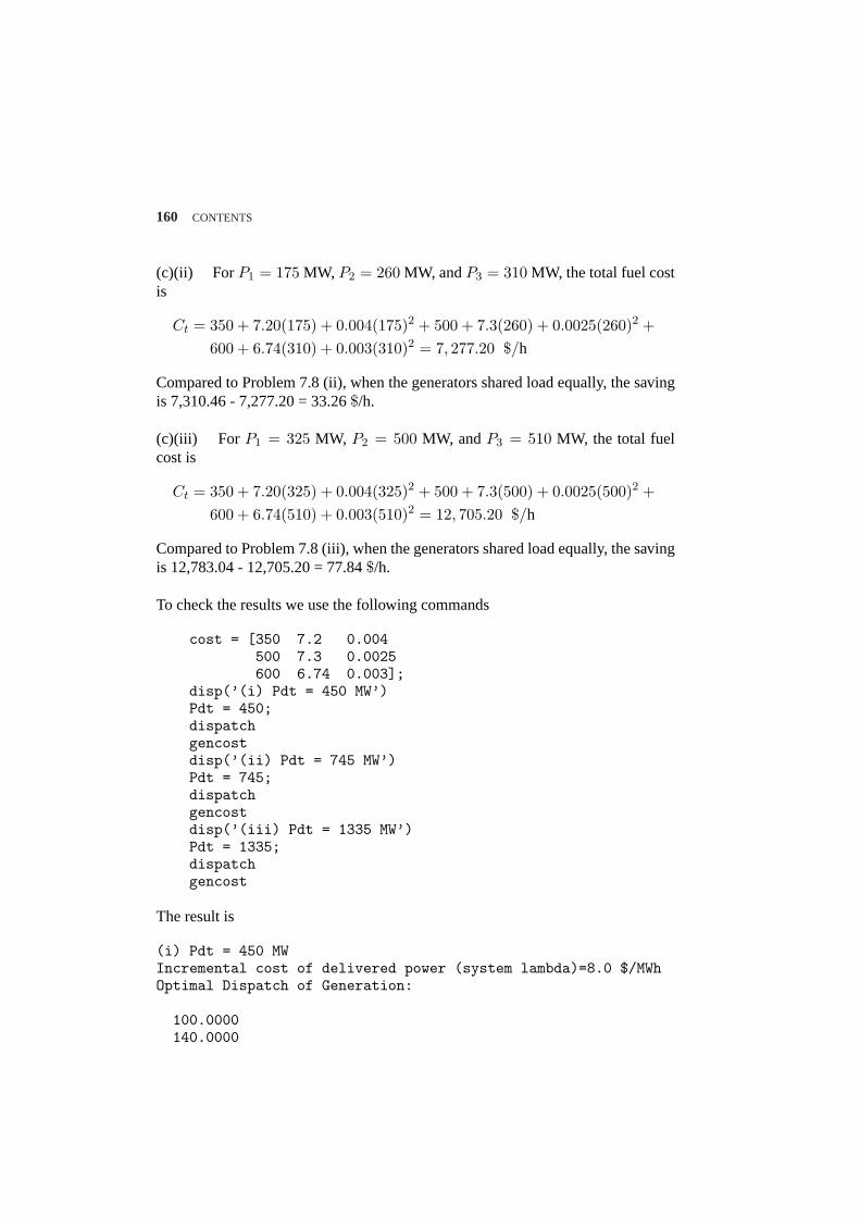
160 CONTENTS
(c)(ii) For P1 = 175 MW, P2 = 260 MW, andP3 = 310 MW, the total fuel costis
Ct = 350 + 7.20(175) + 0.004(175)2 + 500 + 7.3(260) + 0.0025(260)2 +600 + 6.74(310) + 0.003(310)2 = 7, 277.20 $/h
Compared to Problem 7.8 (ii), when the generators shared load equally, the savingis 7,310.46 - 7,277.20 = 33.26$/h.
(c)(iii) For P1 = 325 MW, P2 = 500 MW, andP3 = 510 MW, the total fuelcost is
Ct = 350 + 7.20(325) + 0.004(325)2 + 500 + 7.3(500) + 0.0025(500)2 +600 + 6.74(510) + 0.003(510)2 = 12, 705.20 $/h
Compared to Problem 7.8 (iii), when the generators shared load equally, the savingis 12,783.04 - 12,705.20 = 77.84$/h.
To check the results we use the following commands
cost = [350 7.2 0.004500 7.3 0.0025600 6.74 0.003];
disp(’(i) Pdt = 450 MW’)Pdt = 450;dispatchgencostdisp(’(ii) Pdt = 745 MW’)Pdt = 745;dispatchgencostdisp(’(iii) Pdt = 1335 MW’)Pdt = 1335;dispatchgencost
The result is
(i) Pdt = 450 MWIncremental cost of delivered power (system lambda)=8.0 $/MWhOptimal Dispatch of Generation:
100.0000140.0000
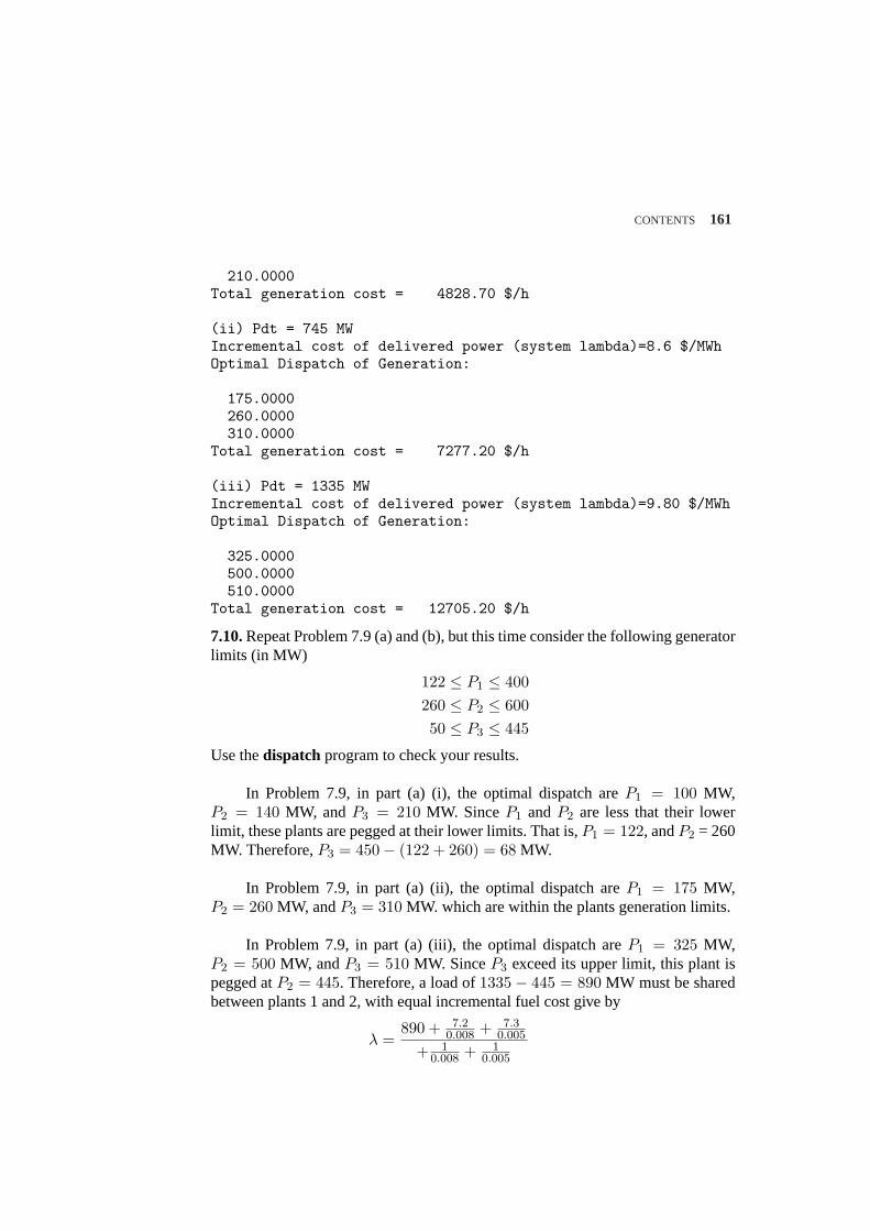
CONTENTS 161
210.0000Total generation cost = 4828.70 $/h
(ii) Pdt = 745 MWIncremental cost of delivered power (system lambda)=8.6 $/MWhOptimal Dispatch of Generation:
175.0000260.0000310.0000
Total generation cost = 7277.20 $/h
(iii) Pdt = 1335 MWIncremental cost of delivered power (system lambda)=9.80 $/MWhOptimal Dispatch of Generation:
325.0000500.0000510.0000
Total generation cost = 12705.20 $/h
7.10.Repeat Problem 7.9 (a) and (b), but this time consider the following generatorlimits (in MW)
122 ≤ P1 ≤ 400260 ≤ P2 ≤ 60050 ≤ P3 ≤ 445
Use thedispatchprogram to check your results.
In Problem 7.9, in part (a) (i), the optimal dispatch areP1 = 100 MW,P2 = 140 MW, and P3 = 210 MW. SinceP1 andP2 are less that their lowerlimit, these plants are pegged at their lower limits. That is,P1 = 122, andP2 = 260MW. Therefore,P3 = 450− (122 + 260) = 68 MW.
In Problem 7.9, in part (a) (ii), the optimal dispatch areP1 = 175 MW,P2 = 260 MW, andP3 = 310 MW. which are within the plants generation limits.
In Problem 7.9, in part (a) (iii), the optimal dispatch areP1 = 325 MW,P2 = 500 MW, andP3 = 510 MW. SinceP3 exceed its upper limit, this plant ispegged atP2 = 445. Therefore, a load of1335− 445 = 890 MW must be sharedbetween plants 1 and 2, with equal incremental fuel cost give by
λ =890 + 7.2
0.008 + 7.30.005
+ 10.008 + 1
0.005
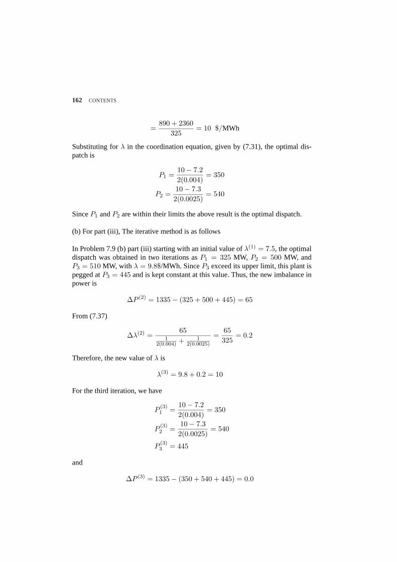
162 CONTENTS
=890 + 2360
325= 10 $/MWh
Substituting forλ in the coordination equation, given by (7.31), the optimal dis-patch is
P1 =10− 7.22(0.004)
= 350
P2 =10− 7.32(0.0025)
= 540
SinceP1 andP2 are within their limits the above result is the optimal dispatch.
(b) For part (iii), The iterative method is as follows
In Problem 7.9 (b) part (iii) starting with an initial value ofλ(1) = 7.5, the optimaldispatch was obtained in two iterations asP1 = 325 MW, P2 = 500 MW, andP3 = 510 MW, with λ = 9.8$/MWh. SinceP3 exceed its upper limit, this plant ispegged atP3 = 445 and is kept constant at this value. Thus, the new imbalance inpower is
∆P (2) = 1335− (325 + 500 + 445) = 65
From (7.37)
∆λ(2) =65
12(0.004) + 1
2(0.0025)
=65325
= 0.2
Therefore, the new value ofλ is
λ(3) = 9.8 + 0.2 = 10
For the third iteration, we have
P(3)1 =
10− 7.22(0.004)
= 350
P(3)2 =
10− 7.32(0.0025)
= 540
P(3)3 = 445
and
∆P (3) = 1335− (350 + 540 + 445) = 0.0
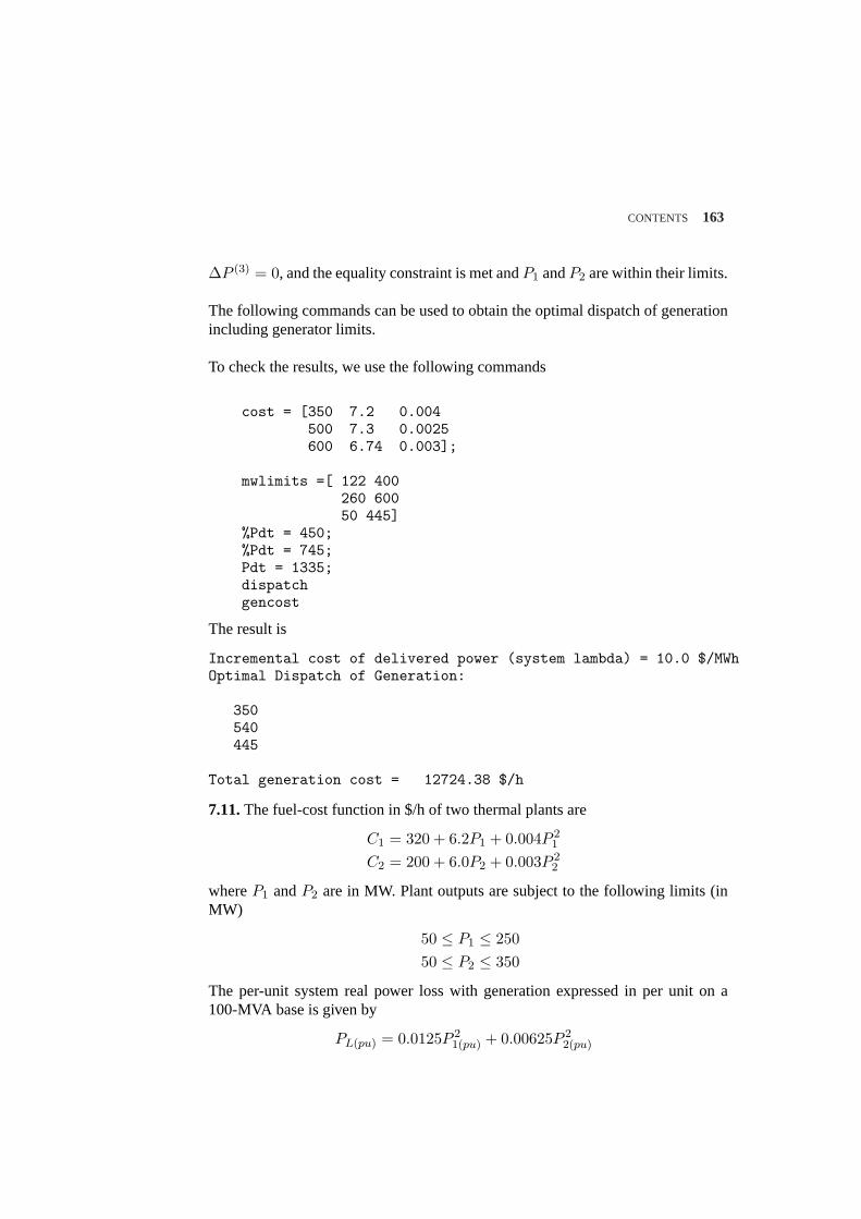
CONTENTS 163
∆P (3) = 0, and the equality constraint is met andP1 andP2 are within their limits.
The following commands can be used to obtain the optimal dispatch of generationincluding generator limits.
To check the results, we use the following commands
cost = [350 7.2 0.004500 7.3 0.0025600 6.74 0.003];
mwlimits =[ 122 400260 60050 445]
%Pdt = 450;%Pdt = 745;Pdt = 1335;dispatchgencost
The result is
Incremental cost of delivered power (system lambda) = 10.0 $/MWhOptimal Dispatch of Generation:
350540445
Total generation cost = 12724.38 $/h
7.11.The fuel-cost function in $/h of two thermal plants are
C1 = 320 + 6.2P1 + 0.004P 21
C2 = 200 + 6.0P2 + 0.003P 22
whereP1 andP2 are in MW. Plant outputs are subject to the following limits (inMW)
50 ≤ P1 ≤ 25050 ≤ P2 ≤ 350
The per-unit system real power loss with generation expressed in per unit on a100-MVA base is given by
PL(pu) = 0.0125P 21(pu) + 0.00625P 2
2(pu)
164 CONTENTS
The total load is 412.35 MW. Determine the optimal dispatch of generation. Startwith an initial estimate ofλ = 7 $/MWh. Use thedispatchprogram to check yourresults.
In the cost functionPi is expressed in MW. Therefore, the real power loss interms of MW generation is
PL =
[0.0125
(P1
100
)2
+ 0.00625(
P2
100
)2]× 100 MW
= 0.000125P 21 + 0.0000625P 2
2 MW
For the numerical solution using the gradient method, assume the initial value ofλ(1) = 7.0. From coordination equations, given by (7.70),P
(1)1 , andP
(1)2 are
P(1)1 =
7.0− 6.22(0.004 + 7.0× 0.000125)
= 82.05128 MW
P(1)2 =
7.0− 6.02(0.003 + 7.0× 0.0000625)
= 145.4545 MW
The real power loss is
P(1)L = 0.000125(82.05228)2 + 0.0000625(145.4545)2 = 2.16386
SincePD = 412.35 MW, the error∆P (1) from (7.68) is
∆P (1) = 412.35 + 2.16386− (82.05128 + 145.4545) = 187.008
From (7.71)
2∑
i=1
(∂Pi
∂λ
)(1)
=0.004 + 0.000125× 6.2
2(0.004 + 7.0× 0.000125)2+
0.003 + 0.0000625× 6.02(0.003 + 7.0× 0.0000625)2
= 243.2701
From (7.65)
∆λ(1) =187.008243.2701
= 0.7687
Therefore, the new value ofλ is
λ(2) = 7.0 + 0.7687 = 7.7687
CONTENTS 165
Continuing the process, for the second iteration, we have
P(2)1 =
7.7687− 6.22(0.004 + 7.7687× 0.000125)
= 157.7848 MW
P(2)2 =
7.7687− 6.02(0.003 + 7.7687× 0.0000625)
= 253.7229 MW
The real power loss is
P(2)L = 0.000125(157.7848)2 + 0.0000625(253.7229)2 = 7.1355
SincePD = 412.35 MW, the error∆P (2) from (7.68) is
∆P (2) = 412.35 + 7.1355− (157.7848 + 253.7229) = 7.9778
From (7.71)
2∑
i=1
(∂Pi
∂λ
)(2)
=0.004 + 0.000125× 6.2
2(0.004 + 7.7687× 0.000125)2+
0.003 + 0.0000625× 6.02(0.003 + 7.7687× 0.0000625)2
= 235.514
From (7.65)
∆λ(2) =7.9778235.514
= 0.0339
Therefore, the new value ofλ is
λ(2) = 7.7687 + 0.0339 = 7.8026
For the third iteration, we have
P(3)1 =
7.8026− 6.22(0.004 + 7.8026× 0.000125)
= 161.0548 MW
P(3)2 =
7.8026− 6.02(0.003 + 7.8026× 0.0000625)
= 258.4252 MW
The real power loss is
P(3)L = 0.000125(161.0548)2 + 0.0000625(258.4252)2 = 7.4163
SincePD = 412.35 MW, the error∆P (3) from (7.68) is
∆P (3) = 412.35 + 7.4163− (161.0548 + 258.4252) = 0.2863
166 CONTENTS
From (7.71)
2∑
i=1
(∂Pi
∂λ
)(3)
=0.004 + 0.000125× 6.2
2(0.004 + 7.8026× 0.000125)2+
0.003 + 0.0000625× 6.02(0.003 + 7.8026× 0.0000625)2
= 235.18
From (7.65)
∆λ(3) =0.2683235.18
= 0.0012
Therefore, the new value ofλ is
λ(3) = 7.8026 + 0.0011 = 7.8038
Continuing the process, the optimal dispatch after six iteration converges toP1 =161.1765 MW, andP2 = 258.6003 MW, with an incremental production cost ofλ = 7.8038$/MWh.
To check the results, we use the following commands
We use the following commands
cost = [320 6.2 0.004200 6.0 0.003];
mwlimits =[ 50 25050 350];
Pdt = 412.35;B=[0.0125 0
0 0.00625]basemva=100;lambda = 7.0;dispatchgencost
The result is
B =
0.0125 00 0.0063
Incremental cost of delivered power (system lambda)= 7.803862 $/MWhOptimal Dispatch of Generation:
161.1765258.6003
Total generation cost = 3375.43 $/h
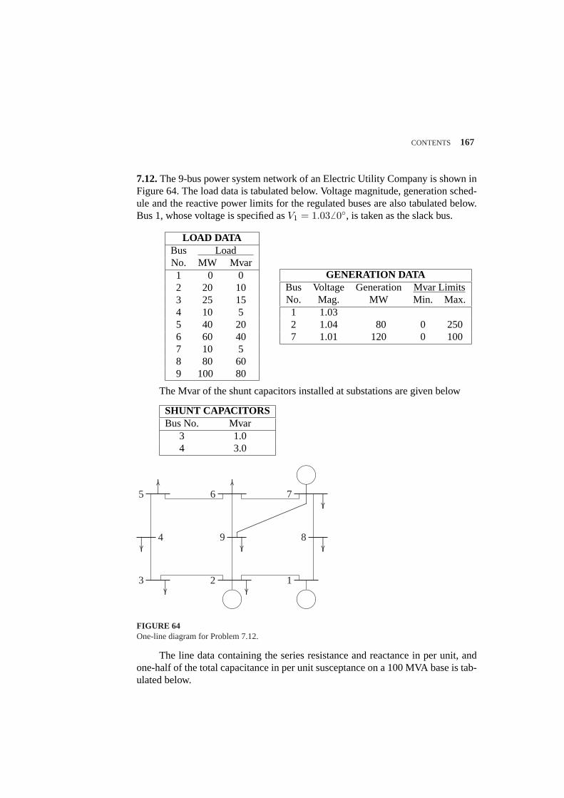
CONTENTS 167
7.12.The 9-bus power system network of an Electric Utility Company is shown inFigure 64. The load data is tabulated below. Voltage magnitude, generation sched-ule and the reactive power limits for the regulated buses are also tabulated below.Bus 1, whose voltage is specified asV1 = 1.03 6 0, is taken as the slack bus.
LOAD DATABus LoadNo. MW Mvar1 0 02 20 103 25 154 10 55 40 206 60 407 10 58 80 609 100 80
GENERATION DATABus Voltage Generation Mvar LimitsNo. Mag. MW Min. Max.1 1.032 1.04 80 0 2507 1.01 120 0 100
The Mvar of the shunt capacitors installed at substations are given below
SHUNT CAPACITORSBus No. Mvar
3 1.04 3.0
........
........
........
........
......................
................
........
........
........
........
......................
................
..............................................
........
........
........
..............................................
........
........
........
..............................................
........
........
........
..............................................
........
........
........
..............................................
........
........
........
..............................................
........
........
........
µ´¶³
µ´¶³
µ´¶³
........
..................................
........................................
........................................
........................................
........................................
.............................................................
5 6 7
4 9 8
3 2 1
FIGURE 64One-line diagram for Problem 7.12.
The line data containing the series resistance and reactance in per unit, andone-half of the total capacitance in per unit susceptance on a 100 MVA base is tab-ulated below.
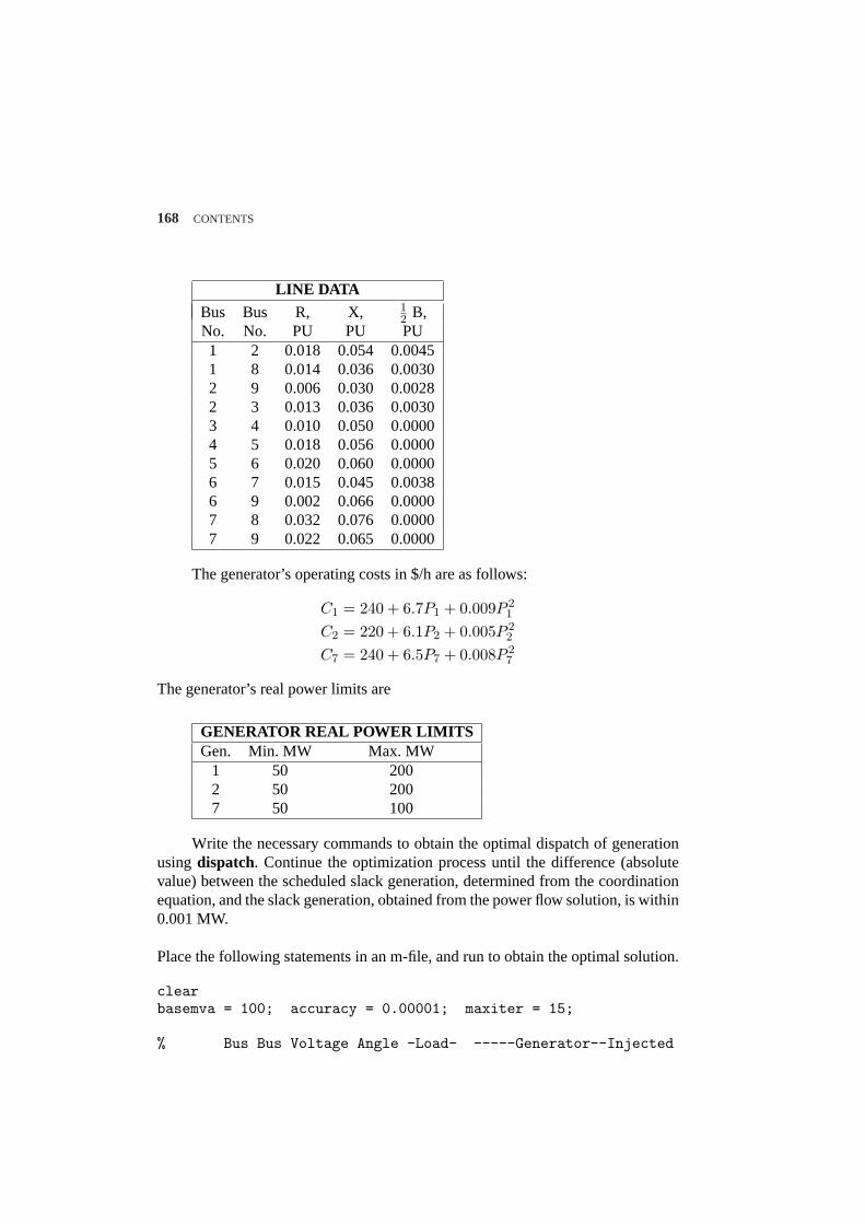
168 CONTENTS
LINE DATABus Bus R, X, 1
2 B,No. No. PU PU PU1 2 0.018 0.054 0.00451 8 0.014 0.036 0.00302 9 0.006 0.030 0.00282 3 0.013 0.036 0.00303 4 0.010 0.050 0.00004 5 0.018 0.056 0.00005 6 0.020 0.060 0.00006 7 0.015 0.045 0.00386 9 0.002 0.066 0.00007 8 0.032 0.076 0.00007 9 0.022 0.065 0.0000
The generator’s operating costs in $/h are as follows:
C1 = 240 + 6.7P1 + 0.009P 21
C2 = 220 + 6.1P2 + 0.005P 22
C7 = 240 + 6.5P7 + 0.008P 27
The generator’s real power limits are
GENERATOR REAL POWER LIMITSGen. Min. MW Max. MW
1 50 2002 50 2007 50 100
Write the necessary commands to obtain the optimal dispatch of generationusingdispatch. Continue the optimization process until the difference (absolutevalue) between the scheduled slack generation, determined from the coordinationequation, and the slack generation, obtained from the power flow solution, is within0.001 MW.
Place the following statements in an m-file, and run to obtain the optimal solution.
clearbasemva = 100; accuracy = 0.00001; maxiter = 15;
% Bus Bus Voltage Angle -Load- -----Generator--Injected
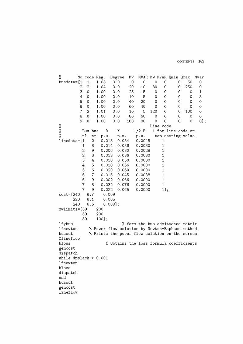
CONTENTS 169
% No code Mag. Degree MW MVAR MW MVAR Qmin Qmax Mvarbusdata=[1 1 1.03 0.0 0 0 0 0 0 50 0
2 2 1.04 0.0 20 10 80 0 0 250 03 0 1.00 0.0 25 15 0 0 0 0 14 0 1.00 0.0 10 5 0 0 0 0 35 0 1.00 0.0 40 20 0 0 0 0 06 0 1.00 0.0 60 40 0 0 0 0 07 2 1.01 0.0 10 5 120 0 0 100 08 0 1.00 0.0 80 60 0 0 0 0 09 0 1.00 0.0 100 80 0 0 0 0 0];
% Line code% Bus bus R X 1/2 B 1 for line code or% nl nr p.u. p.u. p.u. tap setting valuelinedata=[1 2 0.018 0.054 0.0045 1
1 8 0.014 0.036 0.0030 12 9 0.006 0.030 0.0028 12 3 0.013 0.036 0.0030 13 4 0.010 0.050 0.0000 14 5 0.018 0.056 0.0000 15 6 0.020 0.060 0.0000 16 7 0.015 0.045 0.0038 16 9 0.002 0.066 0.0000 17 8 0.032 0.076 0.0000 17 9 0.022 0.065 0.0000 1];
cost=[240 6.7 0.009220 6.1 0.005240 6.5 0.008];
mwlimits=[50 20050 20050 100];
lfybus % form the bus admittance matrixlfnewton % Power flow solution by Newton-Raphson methodbusout % Prints the power flow solution on the screen%lineflowbloss % Obtains the loss formula coefficientsgencostdispatchwhile dpslack > 0.001lfnewtonblossdispatchendbusoutgencostlineflow
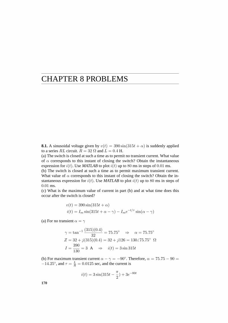
CHAPTER 8 PROBLEMS
8.1.A sinusoidal voltage given byv(t) = 390 sin(315t + α) is suddenly appliedto a seriesRL circuit. R = 32 Ω andL = 0.4 H.(a) The switch is closed at such a time as to permit no transient current. What valueof α corresponds to this instant of closing the switch? Obtain the instantaneousexpression fori(t). UseMATLABto plot i(t) up to80 ms in steps of0.01 ms.(b) The switch is closed at such a time as to permit maximum transient current.What value ofα corresponds to this instant of closing the switch? Obtain the in-stantaneous expression fori(t). UseMATLABto plot i(t) up to80 ms in steps of0.01 ms.(c) What is the maximum value of current in part (b) and at what time does thisoccur after the switch is closed?
v(t) = 390 sin(315t + α)
i(t) = Im sin(315t + α− γ)− Ime−t/τ sin(α− γ)
(a) For no transientα = γ
γ = tan−1 (315)(0.4)32
= 75.75 ⇒ α = 75.75
Z = 32 + j(315)(0.4) = 32 + j126 = 1306 75.75 Ω
I =390130
= 3 A ⇒ i(t) = 3 sin 315t
(b) For maximum transient currentα − γ = −90. Therefore,α = 75.75 − 90 =−14.25, andτ = L
R = 0.0125 sec, and the current is
i(t) = 3 sin(315t− π
2) + 3e−80t
170

CONTENTS 171
(c)
di(t)dt
= (3)(315) cos(315t− π
2)− 240e−80t = 0
Use the command[Imax, k] = max(i), tmax = t(k) to find the maximumvalue of current, and the corresponding time.
imax = 4.371 A
tmax = 0.0096 sec
Save the following statements in a file namedch8p1.m, and run to obtain the plots.
disp(’Problem 8.1’)R = 32; L = 0.4; tau= L/R;w=315; X=w*L;Z=R+j*X; Vm = 390;gama=angle(Z);gamad=gama*180/pi;Im=Vm/130;disp(’(a)’)alpha1= gama; alpha = alpha1*180/pit=0:.0001:.08;i1=Im*sin(315*t+alpha1 -gama);subplot(211), plot(t, i1), gridxlabel(’t, sec’), ylabel(’i(t)’)[I1max,k] = max(i1)tmax= t(k)disp(’(b), (c)’)alpha2=gama - pi/2; alpha = alpha2*180/pii2=Im*sin(315*t+alpha2 -gama)-Im*exp(-t/tau).*sin(alpha2-gama);subplot(212), plot(t, i2), gridxlabel(’t, sec’), ylabel(’i(t)’)[I2max,k] = max(i2)tmax= t(k)
8.2.Consider the synchronous generator in Example 8.2. A three-phase short cir-cuit is applied at the instant when the rotor direct axis position is atδ = 30. Useode45to simulate (8.36), and obtain and plot the transient waveforms for the cur-rent in each phase and the field current.
In Example 8.2, setδ = 30, rename the file and run the program.
8.3.Consider the synchronous generator in Example 8.2. A line-to-line short cir-cuit occurs between phasesb andc at the instant when the rotor direct axis position
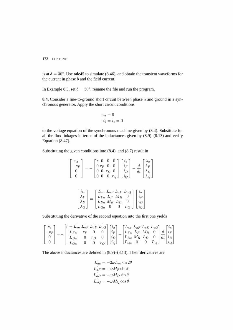
172 CONTENTS
is atδ = 30. Useode45to simulate (8.46), and obtain the transient waveforms forthe current in phaseb and the field current.
In Example 8.3, setδ = 30, rename the file and run the program.
8.4.Consider a line-to-ground short circuit between phasea and ground in a syn-chronous generator. Apply the short circuit conditions
va = 0ib = ic = 0
to the voltage equation of the synchronous machine given by (8.4). Substitute forall the flux linkages in terms of the inductances given by (8.9)–(8.13) and verifyEquation (8.47).
Substituting the given conditions into (8.4), and (8.7) result in
va
−vF
00
= −
r 0 0 00 rF 0 00 0 rD 00 0 0 rQ
iaiFiDiQ
−
d
dt
λa
λF
λD
λQ
λa
λF
λD
λQ
=
Laa LaF LaD LaQ
LFa LF MR 0LDa MR LD 0LQa 0 0 LQ
iaiFiDiQ
Substituting the derivative of the second equation into the first one yields
va
−vF
00
=−
r + ˙Laa˙LaF
˙LaD˙LaQ
˙LFa rF 0 0˙LDa 0 rD 0˙LQa 0 0 rQ
iaiFiDiQ
−
Laa LaF LaD LaQ
LFa LF MR 0LDa MR LD 0LQa 0 0 LQ
d
dt
iaiFiDiQ
The above inductances are defined in (8.9)–(8.13). Their derivatives are
˙Laa = −2ωLm sin 2θ˙LaF = −ωMF sin θ˙LaD = −ωMD sin θ˙LaQ = −ωMQ cos θ
CONTENTS 173
Substituting for the inductances, we obtain
0−vF
00
=
−
r − 2ωLm sin 2θ−ωMF sin θ−ωMD sin θωMQ cos θ−ωMF sin θ rF 0 0−ωMD sin θ 0 rD 0ωMQ cos θ 0 0 rQ
iaiFiDiQ
−
Ls+Lm cos 2θMF cos θMD cos θMQ sin θMF cos θ LF MR 0MD cos θ MR LD 0MQ sin θ 0 0 LQ
d
dt
iaiFiDiQ
where
Ls =13(L0 + Ld + Lq)
Lm =13(Ld − Lq)
8.5. Consider the synchronous generator in Example 8.2. A line-to-ground shortcircuit occurs between phasea and ground at the instant when the rotor direct axisposition is atδ = 30. Useode45to simulate (8.47), and obtain the transient wave-forms for the current in phasea and the field current.
In Example 8.4, setδ = 30, rename the file and run the program.
8.6.A three-phase, 60-Hz synchronous machine is driven at constant synchronousspeed by a prime mover. The armature windings are initially open-circuited andfield voltage is adjusted so that the armature terminal voltage is at the rated value(i.e., 1.0 per unit). The machine has the following per unit reactances and timeconstants.
X ′′d = 0.25 pu τ ′′d = 0.04 sec
X ′d = 0.45 pu τ ′d = 1.4 sec
Xd = 1.50 pu
(a) Determine the steady state, transient, and subtransient short circuit currents.(b) Obtain and plot the fundamental-frequency waveform of the armature currentfor a three-phase short circuit at the terminals of the generator. Assume the shortcircuit is applied at the instant when the rotor direct axis is along the magnetic axis
174 CONTENTS
of phasea, i.e.,δ = 0.
(a)
Id =E0
Xd=
1.01.5
= 0.6667 pu
I ′d =E0
X ′d
=1.00.45
= 2.2222 pu
I ′′d =E0
X ′′d
=1.00.25
= 4.0 pu
(b) From (8.57), we have
iac(t)=√
2(1)[(
10.25
− 10.45
)e−t/0.04+
(1
0.45− 1
1.5
)e−t/1.4+
11.5
]sinωt
iac(t) =[2.5142e−25t + 2.2e−0.7143t + 0.9428
]sinωt
Use the following statements to obtain the short-circuit plot.
disp(’Problem 8.6’)w0 = 2*pi*60; E0 = 1.0; delta = 0;Xd2dash = 0.25; Xddash = 0.45; Xd = 1.5;tau2dash = 0.04; taudash = 1.4;t=0:1/(4*240):.34;iac = sqrt(2)*E0*((1/Xd2dash-1/Xddash)*exp(-t/tau2dash) +...
(1/Xddash-1/Xd)*exp(-t/taudash) + 1/Xd).*sin(w0*t + delta);di1 = sqrt(2)*E0*((1/Xd2dash-1/Xddash)*exp(-t/tau2dash) +...
(1/Xddash-1/Xd)*exp(-t/taudash) + 1/Xd);di2 = sqrt(2)*E0*((1/Xddash-1/Xd)*exp(-t/taudash)+1/Xd);di3=sqrt(2)*E0/Xd*ones(1,length(t));plot(t, iac, t, di1, t, di2, t, di3), gridxlabel(’t, sec’), ylabel(’iac, A’)[t’ iac’]
8.7.For the machine in Problem 8.6, assume that a three-phase short circuit is ap-plied at the instant when the rotor quadrature axis is along the magnetic axis ofphasea, i.e.,δ = π/2 radians. Obtain and plot the asymmetrical waveform of thearmature current for phasea. The armature short circuit time constant isτa = 0.3sec.
From (8.59), we have
Idc =√
2E0
X ′′d
sin δ e−t/τa
=√
21
0.25(1)e−3.3333t = 5.6568e−3.3333t
CONTENTS 175
The asymmetrical short circuit current is
iasy(t) =[2.5142e−25t + 2.2e−0.7143t + 0.9428
]sin(ωt +
π
2) + 5.6568e−3.3333t
8.8.A three-phase, 60-Hz synchronous machine is driven at constant synchronousspeed by a prime mover. The armature windings are initially open-circuited andfield voltage is adjusted so that the armature terminal voltage is at the rated value(i.e., 1.0 per unit). The generator is suddenly subjected to a symmetrical three-phase short circuit at the instant when direct axis is along the magnetic axis ofphasea, i.e.,δ = 0. An oscillogram of the short-circuited current is obtained. Thepeak values at the first two cycles, at the 20th and 21st cycles, and the steady valueafter a long time were recorded as tabulated in the following table.
Imax, pu 5.4016 4.6037 · · · 2.6930 2.6720 · · · 0.9445Time, sec 0.0042 0.0208 · · · 0.3208 0.3375 · · · 10.004
Determine the transient and the subtransient reactances and time constants.
The following statements are written with reference to the procedure in Section(8.9).
disp(’Problem 8.8’)E0 = 1.0;Im=[5.4016 4.6037 2.6930 2.6720 0.9445];t=[0.0042 0.0208 0.3208 0.3375 10.004];
I = Im/sqrt(2); % The rms value of the above envelopid=I(5); % rms value of the steady short-circuitDt2 =[t(3) t(4)]; % First two cyclesDi2 = I(3)-id I(4)-id];%Diff. between transient envelop and idLDi2= log(Di2); %Natural log of the above two pointsc2=polyfit(Dt2, LDi2, 1);%Finds coefficients of the polynomial
% i.e. the slope and intercept of a straight lineiddash=(exp(c2(2))+id) % rms value of the transient currentXddash=E0/iddash % Direct-axis transient reactancetaudash=abs(1/c2(1)) % Short-circuit transient time constantDi=(iddash-id)*[exp(-t(1)/taudash) exp(-t(2)/taudash)];Di1=[I(1)-Di(1)-id I(2)-Di(2)-id]; % Subtransient envelopLDi1=log(Di1);Dt1 =[t(1) t(2)]; % Natural log of the first two pointsc1=polyfit(Dt1, LDi1, 1);%Finds coefficients of the polynomial
% i.e. the slope and intercept of a straight lineid2dash=exp(c1(2))+iddash %rms value of subtransient currentXd2dash= E0/id2dash % Direct-axis subtransient reactancetau2dash=abs(1/c1(1))%Short-circuit subtransient time constant
176 CONTENTS
t=0:.005:.045;fit2 = polyval(c2, t); % line C2 evaluated for all values of tfit1 = polyval(c1, t); line C1 evaluated for all values of tplot(t, fit1, t, fit2),grid % Logarithmic plot of id’’ and id’ylabel(’Ln(I), pu’) % intercepts are ln(Id’’) and Ln(Id’)xlabel(’t, sec’) % slopes are the reciprocal of the
% time constants
The result is
I ′d = 2.2273 pu X ′d = 0.4490; pu τ ′d = 1.3821 sec
I ′′d = 4.0024 pu X ′′d = 0.2498; pu τ ′′d = 0.0397 sec
8.9. A 100-MVA, three-phase, 60-Hz generator driven at constant speed has thefollowing per unit reactances and time constants
X ′′d = 0.20 pu τ ′′d = 0.04 sec
X ′d = 0.30 pu τ ′d = 1.0 sec
Xd = 1.20 pu τa = 0.25 sec
The armature windings are initially open-circuited and field voltage is ad-justed so that the armature terminal voltage is at the rated value (i.e., 1.0 per unit).The generator is suddenly subjected to a symmetrical three-phase short circuit atthe instant whenδ = π/2. Obtain and plot the asymmetrical waveform of the ar-mature current for phase a. Determine
(a) The rms value of the ac component in phasea at t = 0.(b) The dc component of the current in phasea at t = 0.(c) The rms value of the asymmetrical current in phasea at t = 0.
Id =E0
Xd=
1.01.2
= 0.8333 pu
I ′d =E0
X ′d
=1.00.3
= 3.3333 pu
I ′′d =E0
X ′′d
=1.00.2
= 5.0 pu
From (8.57), we have
iac(t)=√
2(1)[(5− 3.3333)e−t/0.04 (3.3333− 0.8333) e−t + 0.8333
]sin(ωt +
π
2)
iac(t) =[2.3571e−25t + 3.5355e−t + 1.1785
]sin(ωt +
π
2)
CONTENTS 177
From (8.59), we have
Idc =√
2(5)(1)e−4t = 7.0711e−4t pu
Use the following statements to obtain the short-circuit plot.
disp(’Problem 8.9’)w0 = 2*pi*60; E0 = 1.0; delta = pi/2;Xd2dash = 0.2; Xddash = 0.3; Xd = 1.2;tau2dash = 0.04; taudash = 1.0; taua=0.25;t=0:1/(4*240):.34;%t=1/240:1/60: 1;iac = sqrt(2)*E0*((1/Xd2dash-1/Xddash)*exp(-t/tau2dash) +...(1/Xddash-1/Xd)*exp(-t/taudash) + 1/Xd).*sin(w0*t + delta);
iasy=iac+sqrt(2)*E0/Xd2dash*sin(delta)*exp(-t/taua);plot(t, iasy), gridxlabel(’t, sec’), ylabel(’iac, A’)[t’ iasy’]
(a) At t = 0, ˆiac = 2.3571+3.5355+1.1785 = 7.0711 pu. Therefore,Iac rms = 5pu.(b) At t = 0, Idc = 7.011(c) At t = 0, the rms value of the asymmetrical current in phase a is
Iasym =√
52 + (7.0711)2 = 8.66 pu
8.10.A 100-MVA, 20-kV, 60-Hz three-phase synchronous generator is connectedto a 100-MVA, 20/400 kV three-phase transformer. The machine has the followingper unit reactances and time constants.
X ′′d = 0.15 pu τ ′′d = 0.035 sec
X ′d = 0.25 pu τ ′d = 0.50 sec
Xd = 1.25 pu τa = 0.3 sec
The transformer reactance is 0.25 per unit. The generator is operating at therated voltage and no-load when a three-phase short circuit occurs at the secondaryterminals of the transformer.(a) Find the subtransient, transient, and the steady state short circuit currents in perunit and actual amperes on both sides of the transformer.(b) What is the maximum asymmetrical rms current (ac plus dc) at the beginningof the short circuit?(c) Obtain and plot the instantaneous expression for the short circuit current includ-ing the dc component. Assumeδ = π/2 radians.
178 CONTENTS
(a) The base current on the generator side is
IB1 =SB√3 VB1
=100× 103
√3 20
= 2886.75 A
The base current on the secondary side of the transformer is
IB2 =20400
(2886.75) = 144.3375 A
the subtransient, transient and the steady state short circuit currents are
I ′′d =1.0
0.15 + 0.25= 2.5 pu = 7, 216.88 A on the generator side
= 360.84 A on the 400-kV side
I ′d =1.0
0.25 + 0.25= 2.0 pu = 5.773.5 A on the generator side
= 288.675 A on the 400-kV side
Id =1.0
1.25 + 0.25= 0.0.6667 pu = 1, 924.5 A on the generator side
= 96.225 A on the 400-kV side
(b) The maximum rms current (ac plus dc) at the beginning of the fault is
Iasy =√
3 I ′′d =√
3 (2.5) = 4.33 pu = 12, 500 A on the generator side
(c) The instantaneous short circuit current including the dc component from (8.60),for δ = π/2 is
i(t)=√
2[(I ′′d−I ′d)e−t/0.4+(I ′d−Id)e−t/1.1+Id] sin(377t + π/2)+
√2I ′′d e−t/0.25
or
i(t) = [0.7071e−28.57t + 1.8856e−2t + 0.9428] sin(377t + π/2) + 3.5355e−3.333t pu
Use the following commands to obtain the solution and a plot ofi(t).
disp(’problem 8.10’)Xd = 1.25; Xd1d = 0.25; Xd2d = 0.15; Xt = 0.25;SB = 100; VL1 = 20; VL2 = 400;IB1 = SB*1000/(sqrt(3)*VL1);IB2 = VL1/VL2*IB1;Id2d = 1.0/(Xd2d+Xt);disp([’Id2dash = ’, num2str(Id2d) ’pu ’,num2str(Id2d*IB1),...
’A ’,num2str(Id2d*IB2), ’A’])Id1d = 1.0/(Xd1d+Xt);
CONTENTS 179
disp([’Id1dash = ’, num2str(Id1d) ’pu ’,num2str(Id1d*IB1),...’A ’,num2str(Id1d*IB2), ’A’])
Id = 1.0/(Xd+Xt);disp([’Id = ’, num2str(Id) ’pu ’, num2str(Id*IB1),...
’A ’,num2str(Id*IB2), ’A’])Iasy = sqrt(3)*Id2d;disp([’Iasy = ’, num2str(Iasy) ’pu ’,num2str(Iasy*IB1),...
’A ’,num2str(Iasy*IB2), ’A’])
t=0:.02:6;it = sqrt(2)*( (Id2d-Id1d)*exp(-t/0.035) + (Id1d-Id)*exp...
(-t/0.5)+Id ).*sin(377*t+pi/2)+sqrt(2)*Id2d*exp(-t/0.3);plot(t, it), gridxlabel(’t, sec’), ylabel(’i, A’)title(’Short circuit current including dc component’)
8.11.In Problem 8.10, a three-phase load of 80-MVA, 0.8 power factor lagging isconnected to the transformer secondary side. The line-to-line voltage at the loadterminals is 400 kV. A three-phase short circuit occurs at the load terminals. Findthe generator transient current including the load current.
The load may be represented by a per unit impedance.
SL =806 36.87
100= 0.86 36.87 pu
V =400400
= 1 6 0 pu
ZL =|V 2|S∗
=1
0.86 −36.87= 1.0 + j0.75 pu
Before fault, the load current is
IL =V
ZL=
1.06 0
1.0 + j0.75= 0.64− j0.48 = 16 −36.87 pu
The emf behind transient reactance is
E′=V +j(X ′d + Xt)IL
=1.06 0 + j(0.25 + 0.25)(0.64− j0.48)=1.24 + j0.32=1.2806 6 14.47 pu
When the fault is applied by closing switch S, the generator short circuit transientcurrent is
I ′g =E′
j(X ′d + Xt)
=1.24 + j0.32
j(0.25 + 0.25)= 0.64− j2.4 = 2.56 6 −75.53 pu
= 7, 393.696 −75.53 A
180 CONTENTS
8.12.A 100-MVA, 20-kV synchronous generator is connected through a transmis-sion line to a 100-MVA, 20-kV synchronous motor. The per unit transient reac-tances of the generator and motor are 0.25 and 0.20, respectively. The line reac-tance on the base of 100 MVA is 0.1 per unit. The motor is taking 50 MW at 0.8power factor leading at a terminal voltage of 20 kV. A three-phase short circuitoccurs at the generator terminals. Determine the transient currents in each of thetwo machines and in the short circuit.
Sm =500.8
6 −36.87 MVA = 0.6256 −36.87 pu
Vm =206 0
20= 1.06 0 pu
I =S∗mV ∗
m
= 0.6256 36.87 pu
The generator emf behind transient reactance is
E′g = Vm + j(X ′
dg + XL)I = 1.0 6 0 + j(0.25 + 0.10)(0.5 + j0.375)= 0.8688 + j0.1750 = 0.88626 11.389 pu
The motor emf behind transient reactance is
E′m = Vm − j(X ′
dm)I = 1.06 0 − j(0.20)(0.5 + j0.375)= 1.075− j0.10 = 1.07966 −5.3145 pu
I ′g =E′
g
j(X ′dg)
=0.88626 11.389
j0.25= 0.7− j3.475 = 3.5456 −78.61 pu
I ′m =E′
m
j(X ′dm + XL)
=1.07966 −5.3145
j0.30= −0.3333− j3.5833
= 3.59886 −95.3145 pu
The short-circuit current is
If = I ′g + I ′m = (0.70− j3.475) + (−0.3333− j3.58333)= 7.06796 −87.026 pu
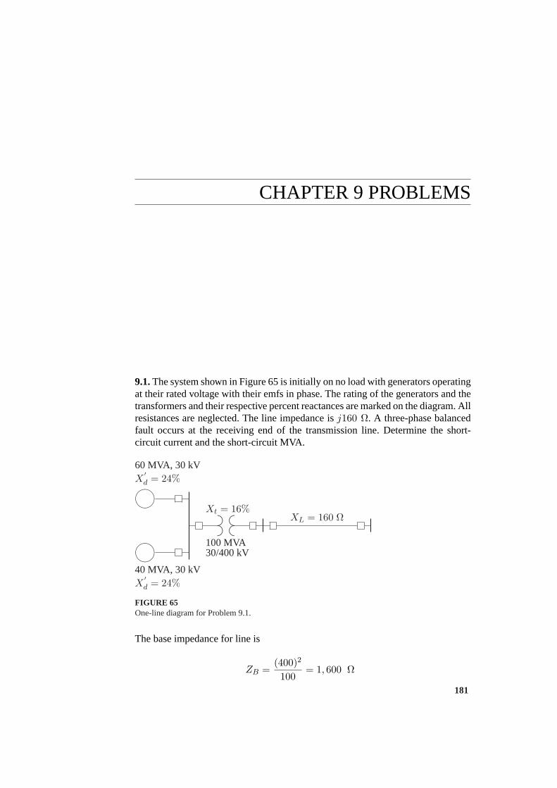
CHAPTER 9 PROBLEMS
9.1.The system shown in Figure 65 is initially on no load with generators operatingat their rated voltage with their emfs in phase. The rating of the generators and thetransformers and their respective percent reactances are marked on the diagram. Allresistances are neglected. The line impedance isj160 Ω. A three-phase balancedfault occurs at the receiving end of the transmission line. Determine the short-circuit current and the short-circuit MVA.
µ´¶³
µ´¶³ ................
........
.............................................................. ......................................................................................
60 MVA, 30 kVX′d = 24%
40 MVA, 30 kVX′d = 24%
Xt = 16%
100 MVA30/400 kV
XL = 160 Ω
FIGURE 65One-line diagram for Problem 9.1.
The base impedance for line is
ZB =(400)2
100= 1, 600 Ω
181
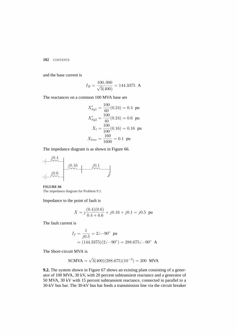
182 CONTENTS
and the base current is
IB =100, 000√
3(400)= 144.3375 A
The reactances on a common 100 MVA base are
X ′dg1 =
10060
(0.24) = 0.4 pu
X ′dg2 =
10040
(0.24) = 0.6 pu
Xt =100100
(0.16) = 0.16 pu
Xline =1601600
= 0.1 pu
The impedance diagram is as shown in Figure 66.
....................................
..........................................
....................................
..........................................
....................................
.......................................... ..........
....................................................
.............................................................................
......................
j0.4
j0.6
j0.16 j0.1
FIGURE 66The impedance diagram for Problem 9.1.
Impedance to the point of fault is
X = j(0.4)(0.6)0.4 + 0.6
+ j0.16 + j0.1 = j0.5 pu
The fault current is
If =1
j0.5= 2 6 −90 pu
= (144.3375)(26 −90) = 288.6756 −90 A
The Short-circuit MVA is
SCMVA =√
3(400)(288.675)(10−3) = 200 MVA
9.2.The system shown in Figure 67 shows an existing plant consisting of a gener-ator of 100 MVA, 30 kV, with 20 percent subtransient reactance and a generator of50 MVA, 30 kV with 15 percent subtransient reactance, connected in parallel to a30-kV bus bar. The 30-kV bus bar feeds a transmission line via the circuit breaker
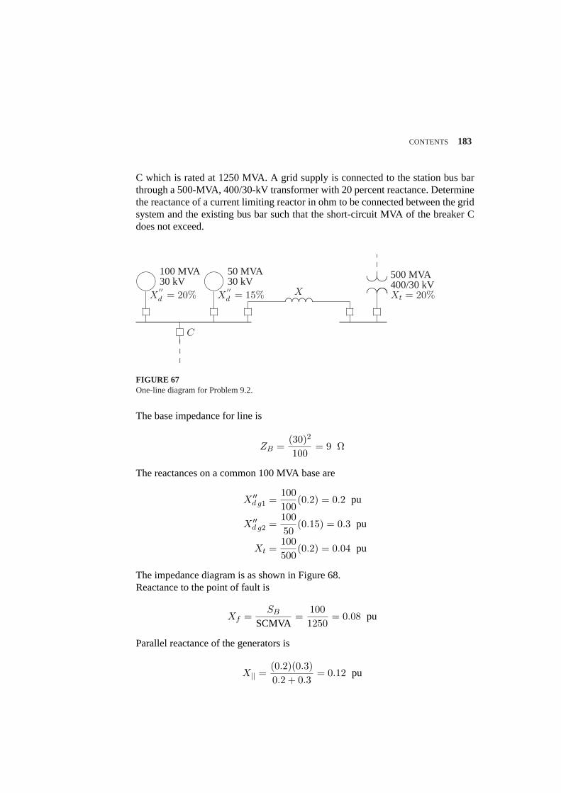
CONTENTS 183
C which is rated at 1250 MVA. A grid supply is connected to the station bus barthrough a 500-MVA, 400/30-kV transformer with 20 percent reactance. Determinethe reactance of a current limiting reactor in ohm to be connected between the gridsystem and the existing bus bar such that the short-circuit MVA of the breaker Cdoes not exceed.
µ´¶³
µ´¶³
.......................................
..........................................................
...................
....................................................
.................................. ...........................................
................................................................................
......
C
........
.....
........
.....
........
.....
........
.....
........
.....
........
.
100 MVA30 kV
X′′d = 20%
50 MVA30 kV
X′′d = 15% X
500 MVA400/30 kVXt = 20%
FIGURE 67One-line diagram for Problem 9.2.
The base impedance for line is
ZB =(30)2
100= 9 Ω
The reactances on a common 100 MVA base are
X ′′d g1 =
100100
(0.2) = 0.2 pu
X ′′d g2 =
10050
(0.15) = 0.3 pu
Xt =100500
(0.2) = 0.04 pu
The impedance diagram is as shown in Figure 68.Reactance to the point of fault is
Xf =SB
SCMVA=
1001250
= 0.08 pu
Parallel reactance of the generators is
X|| =(0.2)(0.3)0.2 + 0.3
= 0.12 pu
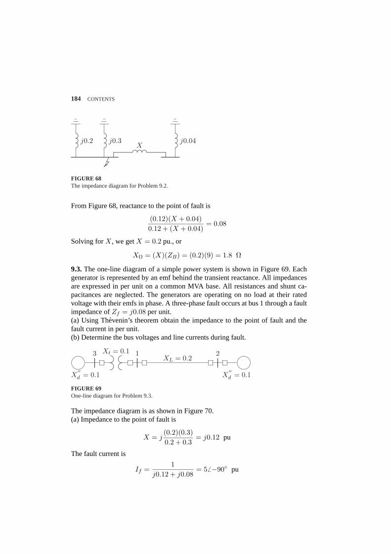
184 CONTENTS
.......................................................................................
j0.2.......................................................................................
j0.3.......................................................................................
j0.04
........
........
............................................................................ .......................................
................................................ ............................................................................................
X
.........................................................................................
FIGURE 68The impedance diagram for Problem 9.2.
From Figure 68, reactance to the point of fault is
(0.12)(X + 0.04)0.12 + (X + 0.04)
= 0.08
Solving forX, we getX = 0.2 pu., or
XΩ = (X)(ZB) = (0.2)(9) = 1.8 Ω
9.3.The one-line diagram of a simple power system is shown in Figure 69. Eachgenerator is represented by an emf behind the transient reactance. All impedancesare expressed in per unit on a common MVA base. All resistances and shunt ca-pacitances are neglected. The generators are operating on no load at their ratedvoltage with their emfs in phase. A three-phase fault occurs at bus 1 through a faultimpedance ofZf = j0.08 per unit.(a) Using Thevenin’s theorem obtain the impedance to the point of fault and thefault current in per unit.(b) Determine the bus voltages and line currents during fault.
µ´¶³
...................................................................................... ...................................................................................... µ´
¶³
X′′d = 0.1
Xt = 0.1
X′′d = 0.1
XL = 0.23 1 2
FIGURE 69One-line diagram for Problem 9.3.
The impedance diagram is as shown in Figure 70.(a) Impedance to the point of fault is
X = j(0.2)(0.3)0.2 + 0.3
= j0.12 pu
The fault current is
If =1
j0.12 + j0.08= 5 6 −90 pu
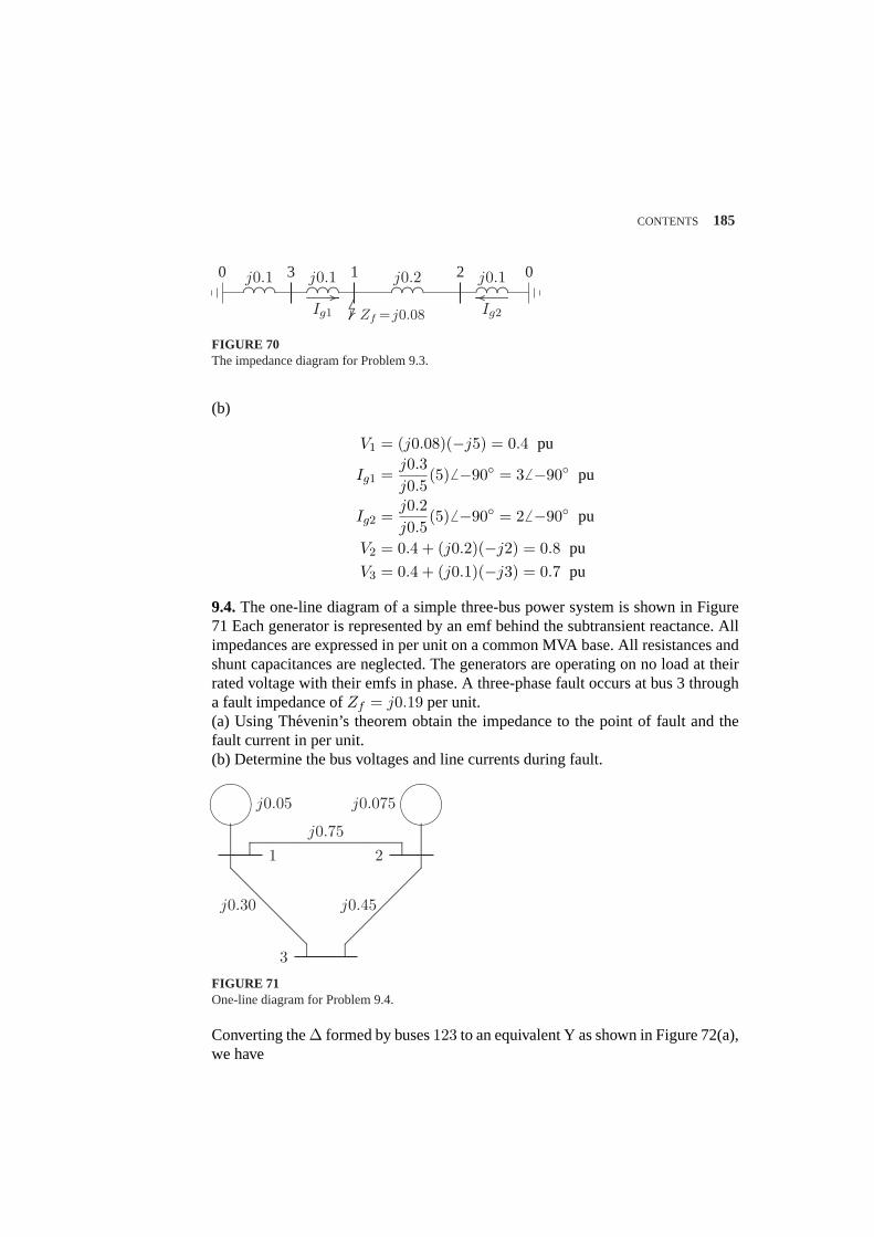
CONTENTS 185
.......................................
................................................ ..........
..........................................................
................... .......................................
................................................ ..........
..........................................................
................................................................................
.......................
j0.1 j0.1 j0.2 j0.10 3 1 2 0....................................................................... ................
Ig1
.......................................................................................
Zf =j0.08 Ig2
FIGURE 70The impedance diagram for Problem 9.3.
(b)
V1 = (j0.08)(−j5) = 0.4 pu
Ig1 =j0.3j0.5
(5)6 −90 = 36 −90 pu
Ig2 =j0.2j0.5
(5)6 −90 = 26 −90 pu
V2 = 0.4 + (j0.2)(−j2) = 0.8 pu
V3 = 0.4 + (j0.1)(−j3) = 0.7 pu
9.4.The one-line diagram of a simple three-bus power system is shown in Figure71 Each generator is represented by an emf behind the subtransient reactance. Allimpedances are expressed in per unit on a common MVA base. All resistances andshunt capacitances are neglected. The generators are operating on no load at theirrated voltage with their emfs in phase. A three-phase fault occurs at bus 3 througha fault impedance ofZf = j0.19 per unit.(a) Using Thevenin’s theorem obtain the impedance to the point of fault and thefault current in per unit.(b) Determine the bus voltages and line currents during fault.
½¼
¾»
½¼
¾»
..........................................................................................................................................................................................................................................................................................
........
........
.................................................................................................................................................................................................................................................................................................
..........................................................................................................................................................................................................................................................................................
1 2
3
j0.05 j0.075
j0.30 j0.45
j0.75
FIGURE 71One-line diagram for Problem 9.4.
Converting the∆ formed by buses123 to an equivalent Y as shown in Figure 72(a),we have
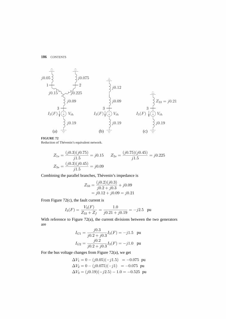
186 CONTENTS
.......................................................................................
.......................................................................................
...................
........
........................................................
.......................
...................
...................
...................................................
....................................
...................
.......................................................................................
m−+
.......................................................................................
.............................................
........
........
........I3(F )
1 2
3
j0.05 j0.075
j0.15 j0.225s
j0.09
Vth
j0.19
(a)
.......................................................................................
.......................................................................................
m−+
.......................................................................................
.............................................
........
........
........I3(F )3
j0.12
j0.09
Vth
j0.19
(b)
.......................................................................................
m−+
.......................................................................................
.............................................
........
........
........I3(F )3
Z33 = j0.21
Vth
j0.19
(c)
FIGURE 72Reduction of Thevenin’s equivalent network.
Z1s =(j0.3)(j0.75)
j1.5= j0.15 Z2s =
(j0.75)(j0.45)j1.5
= j0.225
Z3s =(j0.3)(j0.45)
j1.5= j0.09
Combining the parallel branches, Thevenin’s impedance is
Z33 =(j0.2)(j0.3)j0.2 + j0.3
+ j0.09
= j0.12 + j0.09 = j0.21
From Figure 72(c), the fault current is
I3(F ) =V3(F )
Z33 + Zf=
1.0j0.21 + j0.19
= −j2.5 pu
With reference to Figure 72(a), the current divisions between the two generatorsare
IG1 =j0.3
j0.2 + j0.3I3(F ) = −j1.5 pu
IG2 =j0.2
j0.2 + j0.3I3(F ) = −j1.0 pu
For the bus voltage changes from Figure 72(a), we get
∆V1 = 0− (j0.05)(−j1.5) = −0.075 pu
∆V2 = 0− (j0.075)(−j1) = −0.075 pu
∆V3 = (j0.19)(−j2.5)− 1.0 = −0.525 pu
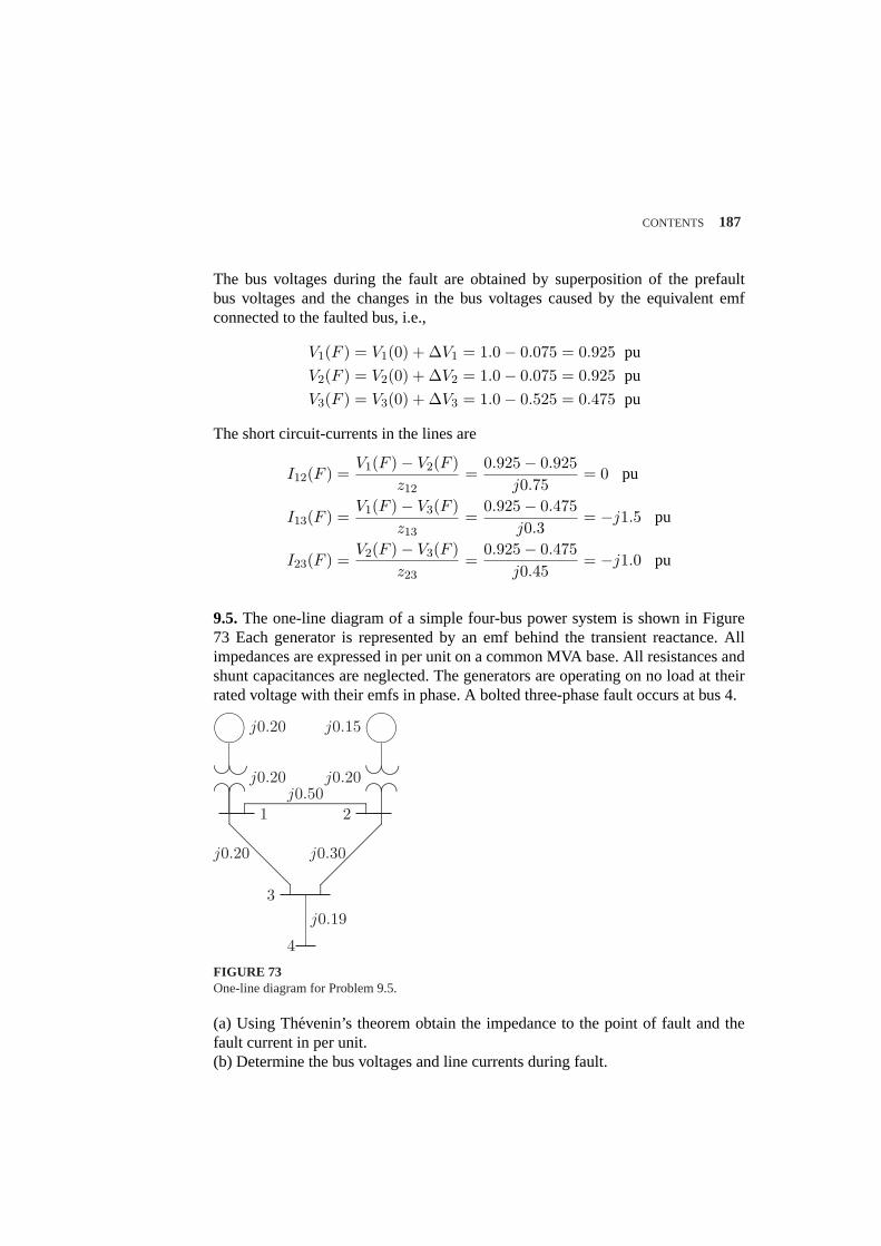
CONTENTS 187
The bus voltages during the fault are obtained by superposition of the prefaultbus voltages and the changes in the bus voltages caused by the equivalent emfconnected to the faulted bus, i.e.,
V1(F ) = V1(0) + ∆V1 = 1.0− 0.075 = 0.925 pu
V2(F ) = V2(0) + ∆V2 = 1.0− 0.075 = 0.925 pu
V3(F ) = V3(0) + ∆V3 = 1.0− 0.525 = 0.475 pu
The short circuit-currents in the lines are
I12(F ) =V1(F )− V2(F )
z12=
0.925− 0.925j0.75
= 0 pu
I13(F ) =V1(F )− V3(F )
z13=
0.925− 0.475j0.3
= −j1.5 pu
I23(F ) =V2(F )− V3(F )
z23=
0.925− 0.475j0.45
= −j1.0 pu
9.5. The one-line diagram of a simple four-bus power system is shown in Figure73 Each generator is represented by an emf behind the transient reactance. Allimpedances are expressed in per unit on a common MVA base. All resistances andshunt capacitances are neglected. The generators are operating on no load at theirrated voltage with their emfs in phase. A bolted three-phase fault occurs at bus 4.
µ´¶³
µ´¶³
................................................................................
.......
..................................................
................................
................................................................................
.......
..................................................
.................................................................................................................................................................................................................................................................
........
........
..................................................................................................................................................................................................................................
.................................................................................................................................................................................................................................
1 2
3
4
j0.20
j0.20
j0.15
j0.20
j0.19
j0.20 j0.30
j0.50
FIGURE 73One-line diagram for Problem 9.5.
(a) Using Thevenin’s theorem obtain the impedance to the point of fault and thefault current in per unit.(b) Determine the bus voltages and line currents during fault.
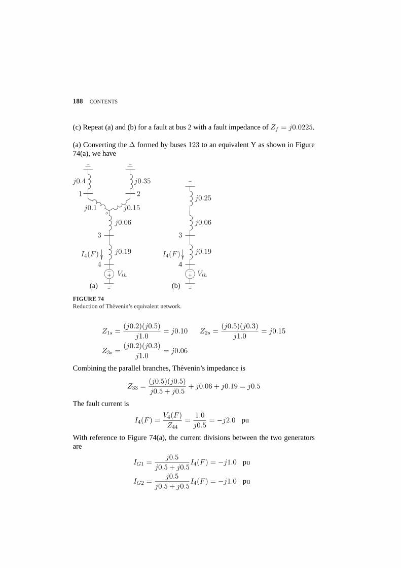
188 CONTENTS
(c) Repeat (a) and (b) for a fault at bus 2 with a fault impedance ofZf = j0.0225.
(a) Converting the∆ formed by buses123 to an equivalent Y as shown in Figure74(a), we have
.......................................................................................
.......................................................................................
...................
........
........................................................
.......................
...................
...................
...................................................
....................................
...................
.......................................................................................
.......................................................................................
m−+
.............................................
........
........
........I4(F )
1 2
3
4
j0.4 j0.35
j0.1 j0.15s
j0.06
Vth
j0.19
(a)
.......................................................................................
.......................................................................................
.......................................................................................
m−+
−+
.............................................
........
........
........I4(F )4
3
j0.25
j0.06
Vth
j0.19
(b)
FIGURE 74Reduction of Thevenin’s equivalent network.
Z1s =(j0.2)(j0.5)
j1.0= j0.10 Z2s =
(j0.5)(j0.3)j1.0
= j0.15
Z3s =(j0.2)(j0.3)
j1.0= j0.06
Combining the parallel branches, Thevenin’s impedance is
Z33 =(j0.5)(j0.5)j0.5 + j0.5
+ j0.06 + j0.19 = j0.5
The fault current is
I4(F ) =V4(F )Z44
=1.0j0.5
= −j2.0 pu
With reference to Figure 74(a), the current divisions between the two generatorsare
IG1 =j0.5
j0.5 + j0.5I4(F ) = −j1.0 pu
IG2 =j0.5
j0.5 + j0.5I4(F ) = −j1.0 pu
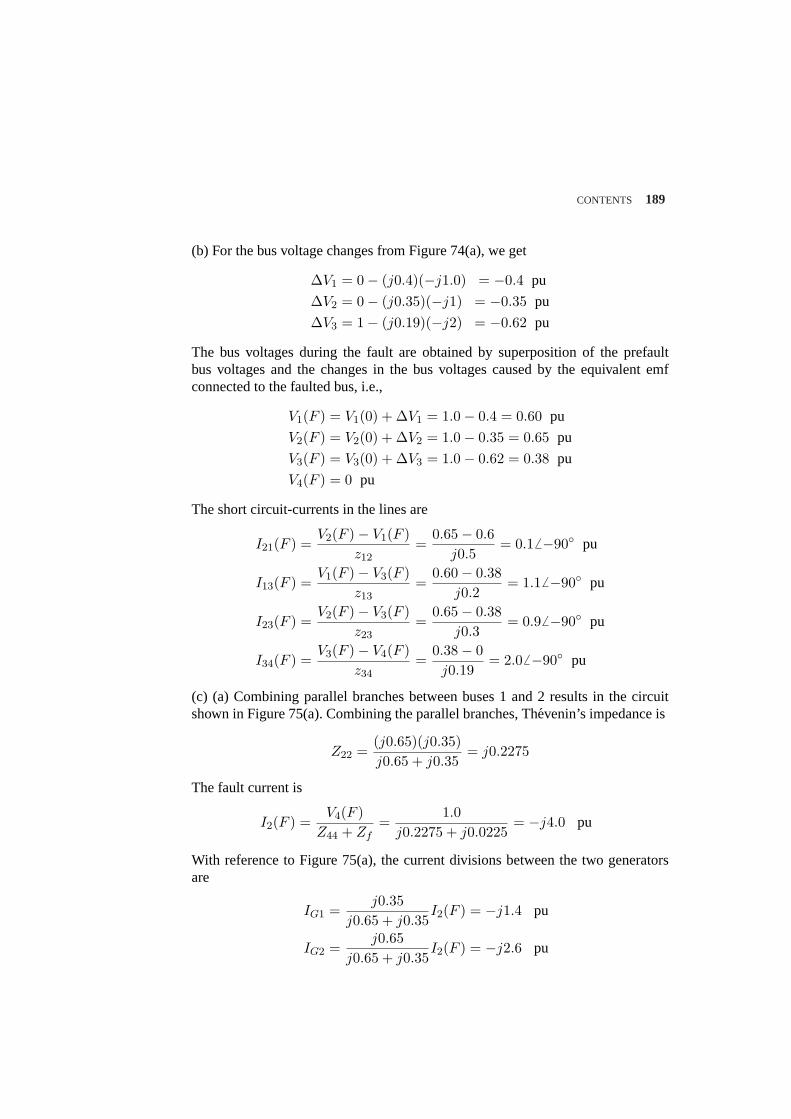
CONTENTS 189
(b) For the bus voltage changes from Figure 74(a), we get
∆V1 = 0− (j0.4)(−j1.0) = −0.4 pu
∆V2 = 0− (j0.35)(−j1) = −0.35 pu
∆V3 = 1− (j0.19)(−j2) = −0.62 pu
The bus voltages during the fault are obtained by superposition of the prefaultbus voltages and the changes in the bus voltages caused by the equivalent emfconnected to the faulted bus, i.e.,
V1(F ) = V1(0) + ∆V1 = 1.0− 0.4 = 0.60 pu
V2(F ) = V2(0) + ∆V2 = 1.0− 0.35 = 0.65 pu
V3(F ) = V3(0) + ∆V3 = 1.0− 0.62 = 0.38 pu
V4(F ) = 0 pu
The short circuit-currents in the lines are
I21(F ) =V2(F )− V1(F )
z12=
0.65− 0.6j0.5
= 0.16 −90 pu
I13(F ) =V1(F )− V3(F )
z13=
0.60− 0.38j0.2
= 1.1 6 −90 pu
I23(F ) =V2(F )− V3(F )
z23=
0.65− 0.38j0.3
= 0.9 6 −90 pu
I34(F ) =V3(F )− V4(F )
z34=
0.38− 0j0.19
= 2.06 −90 pu
(c) (a) Combining parallel branches between buses 1 and 2 results in the circuitshown in Figure 75(a). Combining the parallel branches, Thevenin’s impedance is
Z22 =(j0.65)(j0.35)j0.65 + j0.35
= j0.2275
The fault current is
I2(F ) =V4(F )
Z44 + Zf=
1.0j0.2275 + j0.0225
= −j4.0 pu
With reference to Figure 75(a), the current divisions between the two generatorsare
IG1 =j0.35
j0.65 + j0.35I2(F ) = −j1.4 pu
IG2 =j0.65
j0.65 + j0.35I2(F ) = −j2.6 pu
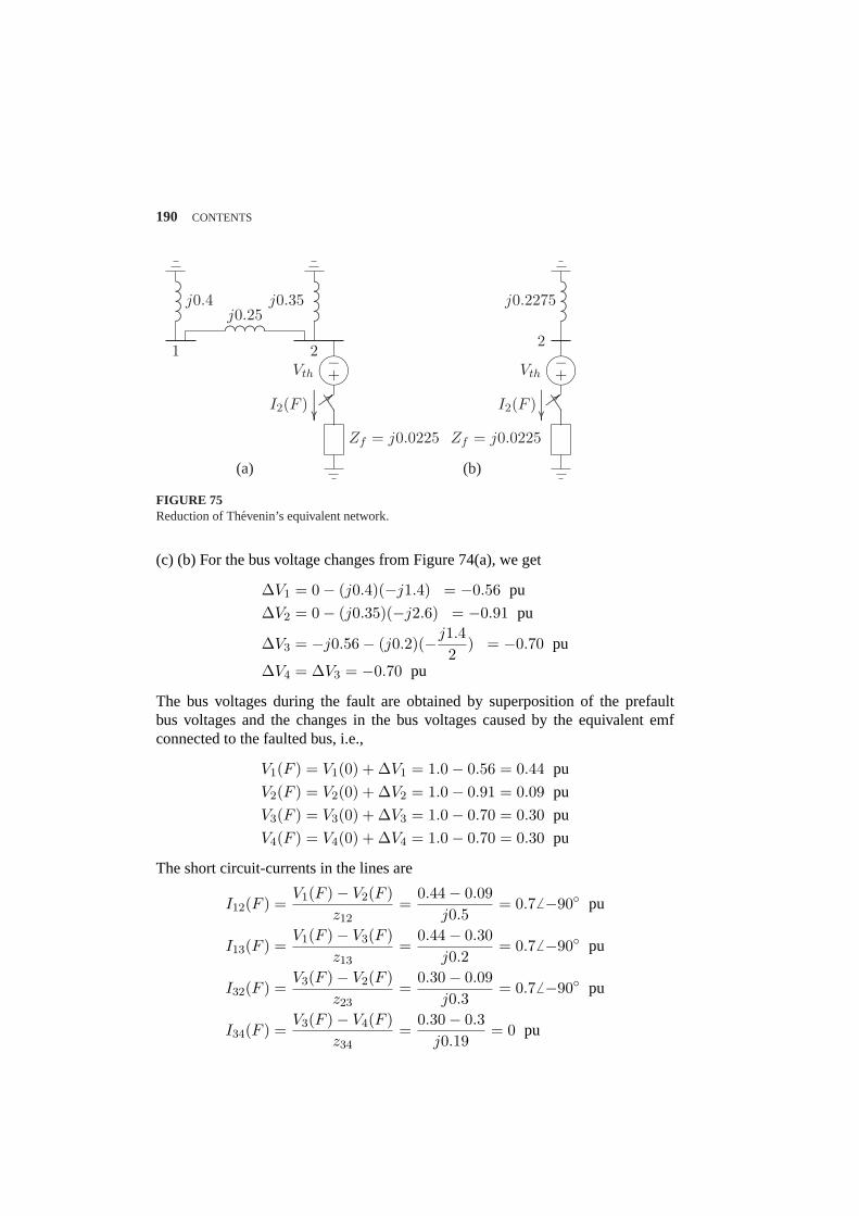
190 CONTENTS
............................................................................................................
............................................................................................................
.....................................
......................................................
.................
µ´¶³
Vth−+
.........................................................
.....................................................
1 2
j0.25j0.4 j0.35
Zf = j0.0225
............................................................
........
........
........I2(F )
(a)
............................................................................................................
µ´¶³−+Vth
.........................................................
Zf = j0.0225
.....................................................
............................................................
........
........
........I2(F )
(b)
2
j0.2275
FIGURE 75Reduction of Thevenin’s equivalent network.
(c) (b) For the bus voltage changes from Figure 74(a), we get
∆V1 = 0− (j0.4)(−j1.4) = −0.56 pu
∆V2 = 0− (j0.35)(−j2.6) = −0.91 pu
∆V3 = −j0.56− (j0.2)(−j1.42
) = −0.70 pu
∆V4 = ∆V3 = −0.70 pu
The bus voltages during the fault are obtained by superposition of the prefaultbus voltages and the changes in the bus voltages caused by the equivalent emfconnected to the faulted bus, i.e.,
V1(F ) = V1(0) + ∆V1 = 1.0− 0.56 = 0.44 pu
V2(F ) = V2(0) + ∆V2 = 1.0− 0.91 = 0.09 pu
V3(F ) = V3(0) + ∆V3 = 1.0− 0.70 = 0.30 pu
V4(F ) = V4(0) + ∆V4 = 1.0− 0.70 = 0.30 pu
The short circuit-currents in the lines are
I12(F ) =V1(F )− V2(F )
z12=
0.44− 0.09j0.5
= 0.7 6 −90 pu
I13(F ) =V1(F )− V3(F )
z13=
0.44− 0.30j0.2
= 0.7 6 −90 pu
I32(F ) =V3(F )− V2(F )
z23=
0.30− 0.09j0.3
= 0.7 6 −90 pu
I34(F ) =V3(F )− V4(F )
z34=
0.30− 0.3j0.19
= 0 pu
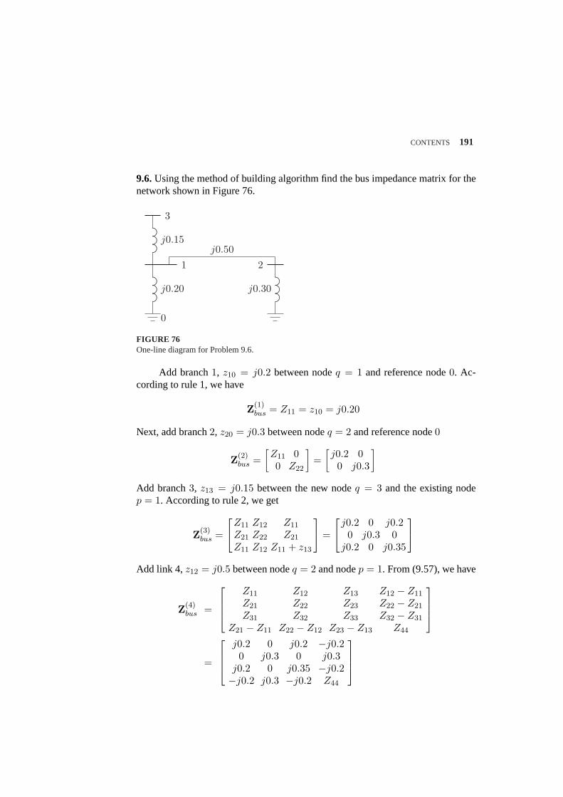
CONTENTS 191
9.6.Using the method of building algorithm find the bus impedance matrix for thenetwork shown in Figure 76.
.........................................................................................................
.........................................................................................................
.........................................................................................................
0
3
1 2
j0.20
j0.15j0.50
j0.30
FIGURE 76One-line diagram for Problem 9.6.
Add branch1, z10 = j0.2 between nodeq = 1 and reference node0. Ac-cording to rule 1, we have
Z(1)bus = Z11 = z10 = j0.20
Next, add branch2, z20 = j0.3 between nodeq = 2 and reference node0
Z(2)bus =
[Z11 00 Z22
]=
[j0.2 00 j0.3
]
Add branch3, z13 = j0.15 between the new nodeq = 3 and the existing nodep = 1. According to rule 2, we get
Z(3)bus =
Z11 Z12 Z11
Z21 Z22 Z21
Z11 Z12 Z11 + z13
=
j0.2 0 j0.20 j0.3 0
j0.2 0 j0.35
Add link 4, z12 = j0.5 between nodeq = 2 and nodep = 1. From (9.57), we have
Z(4)bus =
Z11 Z12 Z13 Z12 − Z11
Z21 Z22 Z23 Z22 − Z21
Z31 Z32 Z33 Z32 − Z31
Z21 − Z11 Z22 − Z12 Z23 − Z13 Z44
=
j0.2 0 j0.2 −j0.20 j0.3 0 j0.3
j0.2 0 j0.35 −j0.2−j0.2 j0.3 −j0.2 Z44
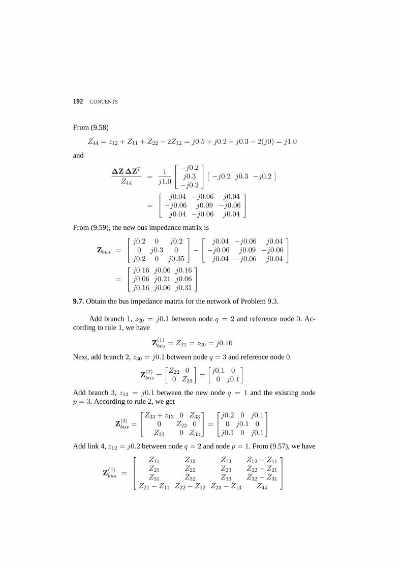
192 CONTENTS
From (9.58)
Z44 = z12 + Z11 + Z22 − 2Z12 = j0.5 + j0.2 + j0.3− 2(j0) = j1.0
and
∆Z∆ZT
Z44=
1j1.0
−j0.2j0.3−j0.2
[ −j0.2 j0.3 −j0.2
]
=
j0.04 −j0.06 j0.04−j0.06 j0.09 −j0.06
j0.04 −j0.06 j0.04
From (9.59), the new bus impedance matrix is
Zbus =
j0.2 0 j0.20 j0.3 0
j0.2 0 j0.35
−
j0.04 −j0.06 j0.04−j0.06 j0.09 −j0.06
j0.04 −j0.06 j0.04
=
j0.16 j0.06 j0.16j0.06 j0.21 j0.06j0.16 j0.06 j0.31
9.7.Obtain the bus impedance matrix for the network of Problem 9.3.
Add branch1, z20 = j0.1 between nodeq = 2 and reference node0. Ac-cording to rule 1, we have
Z(1)bus = Z22 = z20 = j0.10
Next, add branch2, z30 = j0.1 between nodeq = 3 and reference node0
Z(2)bus =
[Z22 00 Z33
]=
[j0.1 00 j0.1
]
Add branch3, z13 = j0.1 between the new nodeq = 1 and the existing nodep = 3. According to rule 2, we get
Z(3)bus =
Z33 + z13 0 Z33
0 Z22 0Z33 0 Z33
=
j0.2 0 j0.10 j0.1 0
j0.1 0 j0.1
Add link 4, z12 = j0.2 between nodeq = 2 and nodep = 1. From (9.57), we have
Z(4)bus =
Z11 Z12 Z13 Z12 − Z11
Z21 Z22 Z23 Z22 − Z21
Z31 Z32 Z33 Z32 − Z31
Z21 − Z11 Z22 − Z12 Z23 − Z13 Z44
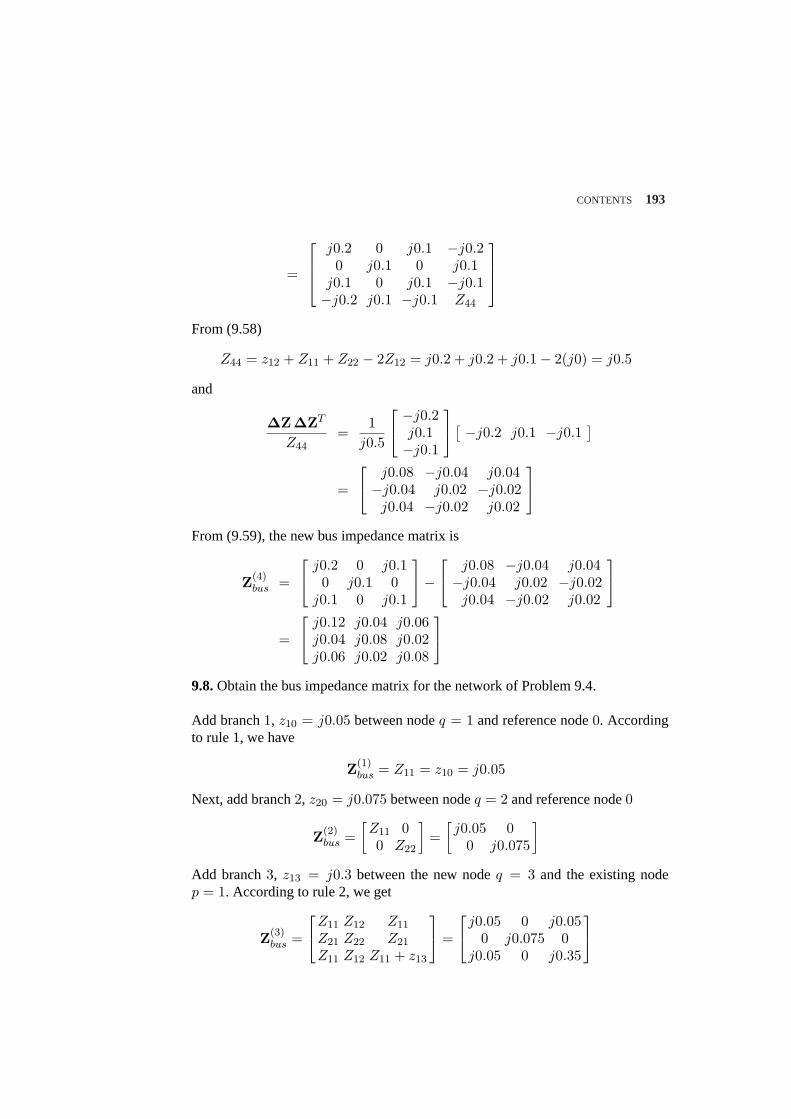
CONTENTS 193
=
j0.2 0 j0.1 −j0.20 j0.1 0 j0.1
j0.1 0 j0.1 −j0.1−j0.2 j0.1 −j0.1 Z44
From (9.58)
Z44 = z12 + Z11 + Z22 − 2Z12 = j0.2 + j0.2 + j0.1− 2(j0) = j0.5
and
∆Z∆ZT
Z44=
1j0.5
−j0.2j0.1−j0.1
[ −j0.2 j0.1 −j0.1
]
=
j0.08 −j0.04 j0.04−j0.04 j0.02 −j0.02
j0.04 −j0.02 j0.02
From (9.59), the new bus impedance matrix is
Z(4)bus =
j0.2 0 j0.10 j0.1 0
j0.1 0 j0.1
−
j0.08 −j0.04 j0.04−j0.04 j0.02 −j0.02
j0.04 −j0.02 j0.02
=
j0.12 j0.04 j0.06j0.04 j0.08 j0.02j0.06 j0.02 j0.08
9.8.Obtain the bus impedance matrix for the network of Problem 9.4.
Add branch1, z10 = j0.05 between nodeq = 1 and reference node0. Accordingto rule 1, we have
Z(1)bus = Z11 = z10 = j0.05
Next, add branch2, z20 = j0.075 between nodeq = 2 and reference node0
Z(2)bus =
[Z11 00 Z22
]=
[j0.05 0
0 j0.075
]
Add branch3, z13 = j0.3 between the new nodeq = 3 and the existing nodep = 1. According to rule 2, we get
Z(3)bus =
Z11 Z12 Z11
Z21 Z22 Z21
Z11 Z12 Z11 + z13
=
j0.05 0 j0.050 j0.075 0
j0.05 0 j0.35
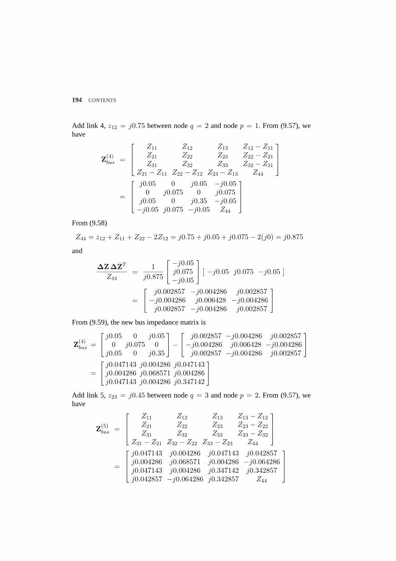
194 CONTENTS
Add link 4, z12 = j0.75 between nodeq = 2 and nodep = 1. From (9.57), wehave
Z(4)bus =
Z11 Z12 Z13 Z12 − Z11
Z21 Z22 Z23 Z22 − Z21
Z31 Z32 Z33 Z32 − Z31
Z21 − Z11 Z22 − Z12 Z23 − Z13 Z44
=
j0.05 0 j0.05 −j0.050 j0.075 0 j0.075
j0.05 0 j0.35 −j0.05−j0.05 j0.075 −j0.05 Z44
From (9.58)
Z44 = z12 + Z11 + Z22 − 2Z12 = j0.75 + j0.05 + j0.075− 2(j0) = j0.875
and
∆Z∆ZT
Z44=
1j0.875
−j0.05j0.075−j0.05
[ −j0.05 j0.075 −j0.05
]
=
j0.002857 −j0.004286 j0.002857−j0.004286 j0.006428 −j0.004286
j0.002857 −j0.004286 j0.002857
From (9.59), the new bus impedance matrix is
Z(4)bus =
j0.05 0 j0.050 j0.075 0
j0.05 0 j0.35
−
j0.002857 −j0.004286 j0.002857−j0.004286 j0.006428 −j0.004286
j0.002857 −j0.004286 j0.002857
=
j0.047143 j0.004286 j0.047143j0.004286 j0.068571 j0.004286j0.047143 j0.004286 j0.347142
Add link 5, z23 = j0.45 between nodeq = 3 and nodep = 2. From (9.57), wehave
Z(5)bus =
Z11 Z12 Z13 Z13 − Z12
Z21 Z22 Z23 Z23 − Z22
Z31 Z32 Z33 Z33 − Z32
Z31 − Z21 Z32 − Z22 Z33 − Z23 Z44
=
j0.047143 j0.004286 j0.047143 j0.042857j0.004286 j0.068571 j0.004286 −j0.064286j0.047143 j0.004286 j0.347142 j0.342857j0.042857 −j0.064286 j0.342857 Z44
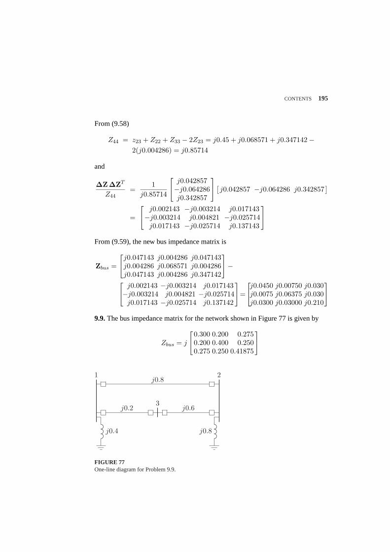
CONTENTS 195
From (9.58)
Z44 = z23 + Z22 + Z33 − 2Z23 = j0.45 + j0.068571 + j0.347142−2(j0.004286) = j0.85714
and
∆Z∆ZT
Z44=
1j0.85714
j0.042857−j0.064286j0.342857
[
j0.042857 −j0.064286 j0.342857]
=
j0.002143 −j0.003214 j0.017143−j0.003214 j0.004821 −j0.025714
j0.017143 −j0.025714 j0.137143
From (9.59), the new bus impedance matrix is
Zbus =
j0.047143 j0.004286 j0.047143j0.004286 j0.068571 j0.004286j0.047143 j0.004286 j0.347142
−
j0.002143 −j0.003214 j0.017143−j0.003214 j0.004821 −j0.025714
j0.017143 −j0.025714 j0.137142
=
j0.0450 j0.00750 j0.030j0.0075 j0.06375 j0.030j0.0300 j0.03000 j0.210
9.9.The bus impedance matrix for the network shown in Figure 77 is given by
Zbus = j
0.300 0.200 0.2750.200 0.400 0.2500.275 0.250 0.41875
.......................................................................................
.......................................................................................
j0.8
j0.2 j0.6
j0.4 j0.8
1 2
3
FIGURE 77One-line diagram for Problem 9.9.
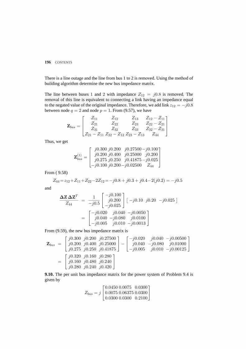
196 CONTENTS
There is a line outage and the line from bus 1 to 2 is removed. Using the method ofbuilding algorithm determine the new bus impedance matrix.
The line between buses1 and 2 with impedanceZ12 = j0.8 is removed. Theremoval of this line is equivalent to connecting a link having an impedance equalto the negated value of the original impedance. Therefore, we add linkz12 = −j0.8between nodeq = 2 and nodep = 1. From (9.57), we have
Zbus =
Z11 Z12 Z13 Z12 − Z11
Z21 Z22 Z23 Z22 − Z21
Z31 Z32 Z33 Z32 − Z31
Z21 − Z11 Z22 − Z12 Z23 − Z13 Z44
Thus, we get
Z(1)bus =
j0.300 j0.200 j0.27500−j0.100j0.200 j0.400 j0.25000 j0.200j0.275 j0.250 j0.41875−j0.025
−j0.100 j0.200−j0.02500 Z44
From ( 9.58)
Z44 =z12+Z11+Z22−2Z12 =−j0.8 + j0.3 + j0.4−2(j0.2) = −j0.5
and
∆Z∆ZT
Z44=
1−j0.5
−j0.100
j0.200−j0.025
[ −j0.10 j0.20 −j0.025
]
=
−j0.020 j0.040 −j0.0050
j0.040 −j0.080 j0.0100−j0.005 j0.010 −j0.0013
From (9.59), the new bus impedance matrix is
Zbus =
j0.300 j0.200 j0.27500j0.200 j0.400 j0.25000j0.275 j0.250 j0.41875
−
−j0.020 j0.040 −j0.00500
j0.040 −j0.080 j0.01000−j0.005 j0.010 −j0.00125
=
j0.320 j0.160 j0.280j0.160 j0.480 j0.240j0.280 j0.240 j0.420
9.10.The per unit bus impedance matrix for the power system of Problem 9.4 isgiven by
Zbus = j
0.0450 0.0075 0.03000.0075 0.06375 0.03000.0300 0.0300 0.2100
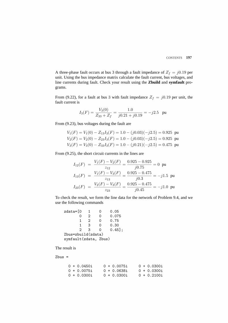
CONTENTS 197
A three-phase fault occurs at bus 3 through a fault impedance ofZf = j0.19 perunit. Using the bus impedance matrix calculate the fault current, bus voltages, andline currents during fault. Check your result using theZbuild andsymfault pro-grams.
From (9.22), for a fault at bus3 with fault impedanceZf = j0.19 per unit, thefault current is
I3(F ) =V3(0)
Z33 + Zf=
1.0j0.21 + j0.19
= −j2.5 pu
From (9.23), bus voltages during the fault are
V1(F ) = V1(0)− Z13I3(F ) = 1.0− (j0.03)(−j2.5) = 0.925 pu
V2(F ) = V2(0)− Z23I3(F ) = 1.0− (j0.03)(−j2.5) = 0.925 pu
V3(F ) = V3(0)− Z33I3(F ) = 1.0− (j0.21)(−j2.5) = 0.475 pu
From (9.25), the short circuit currents in the lines are
I12(F ) =V1(F )− V2(F )
z12=
0.925− 0.925j0.75
= 0 pu
I13(F ) =V1(F )− V3(F )
z13=
0.925− 0.475j0.3
= −j1.5 pu
I23(F ) =V2(F )− V3(F )
z23=
0.925− 0.475j0.45
= −j1.0 pu
To check the result, we form the line data for the network of Problem 9.4, and weuse the following commands
zdata=[0 1 0 0.050 2 0 0.0751 2 0 0.751 3 0 0.302 3 0 0.45];
Zbus=zbuild(zdata)symfault(zdata, Zbus)
The result is
Zbus =
0 + 0.0450i 0 + 0.0075i 0 + 0.0300i0 + 0.0075i 0 + 0.0638i 0 + 0.0300i0 + 0.0300i 0 + 0.0300i 0 + 0.2100i
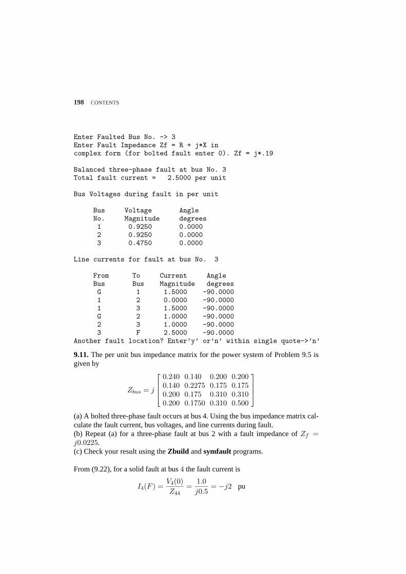
198 CONTENTS
Enter Faulted Bus No. -> 3Enter Fault Impedance Zf = R + j*X incomplex form (for bolted fault enter 0). Zf = j*.19
Balanced three-phase fault at bus No. 3Total fault current = 2.5000 per unit
Bus Voltages during fault in per unit
Bus Voltage AngleNo. Magnitude degrees1 0.9250 0.00002 0.9250 0.00003 0.4750 0.0000
Line currents for fault at bus No. 3
From To Current AngleBus Bus Magnitude degreesG 1 1.5000 -90.00001 2 0.0000 -90.00001 3 1.5000 -90.0000G 2 1.0000 -90.00002 3 1.0000 -90.00003 F 2.5000 -90.0000
Another fault location? Enter’y’ or’n’ within single quote->’n’
9.11.The per unit bus impedance matrix for the power system of Problem 9.5 isgiven by
Zbus = j
0.240 0.140 0.200 0.2000.140 0.2275 0.175 0.1750.200 0.175 0.310 0.3100.200 0.1750 0.310 0.500
(a) A bolted three-phase fault occurs at bus 4. Using the bus impedance matrix cal-culate the fault current, bus voltages, and line currents during fault.(b) Repeat (a) for a three-phase fault at bus 2 with a fault impedance ofZf =j0.0225.(c) Check your result using theZbuild andsymfault programs.
From (9.22), for a solid fault at bus4 the fault current is
I4(F ) =V4(0)Z44
=1.0j0.5
= −j2 pu
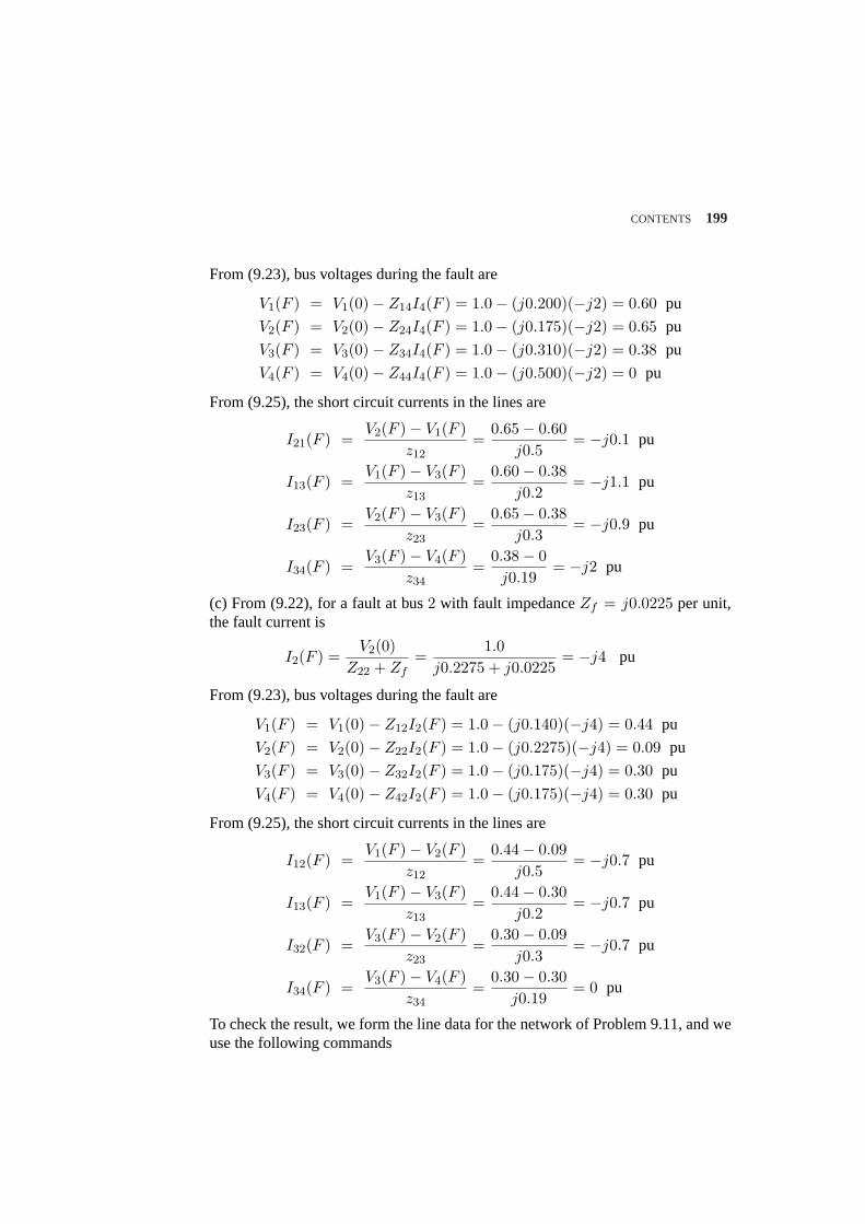
CONTENTS 199
From (9.23), bus voltages during the fault are
V1(F ) = V1(0)− Z14I4(F ) = 1.0− (j0.200)(−j2) = 0.60 pu
V2(F ) = V2(0)− Z24I4(F ) = 1.0− (j0.175)(−j2) = 0.65 pu
V3(F ) = V3(0)− Z34I4(F ) = 1.0− (j0.310)(−j2) = 0.38 pu
V4(F ) = V4(0)− Z44I4(F ) = 1.0− (j0.500)(−j2) = 0 pu
From (9.25), the short circuit currents in the lines are
I21(F ) =V2(F )− V1(F )
z12=
0.65− 0.60j0.5
= −j0.1 pu
I13(F ) =V1(F )− V3(F )
z13=
0.60− 0.38j0.2
= −j1.1 pu
I23(F ) =V2(F )− V3(F )
z23=
0.65− 0.38j0.3
= −j0.9 pu
I34(F ) =V3(F )− V4(F )
z34=
0.38− 0j0.19
= −j2 pu
(c) From (9.22), for a fault at bus2 with fault impedanceZf = j0.0225 per unit,the fault current is
I2(F ) =V2(0)
Z22 + Zf=
1.0j0.2275 + j0.0225
= −j4 pu
From (9.23), bus voltages during the fault are
V1(F ) = V1(0)− Z12I2(F ) = 1.0− (j0.140)(−j4) = 0.44 pu
V2(F ) = V2(0)− Z22I2(F ) = 1.0− (j0.2275)(−j4) = 0.09 pu
V3(F ) = V3(0)− Z32I2(F ) = 1.0− (j0.175)(−j4) = 0.30 pu
V4(F ) = V4(0)− Z42I2(F ) = 1.0− (j0.175)(−j4) = 0.30 pu
From (9.25), the short circuit currents in the lines are
I12(F ) =V1(F )− V2(F )
z12=
0.44− 0.09j0.5
= −j0.7 pu
I13(F ) =V1(F )− V3(F )
z13=
0.44− 0.30j0.2
= −j0.7 pu
I32(F ) =V3(F )− V2(F )
z23=
0.30− 0.09j0.3
= −j0.7 pu
I34(F ) =V3(F )− V4(F )
z34=
0.30− 0.30j0.19
= 0 pu
To check the result, we form the line data for the network of Problem 9.11, and weuse the following commands
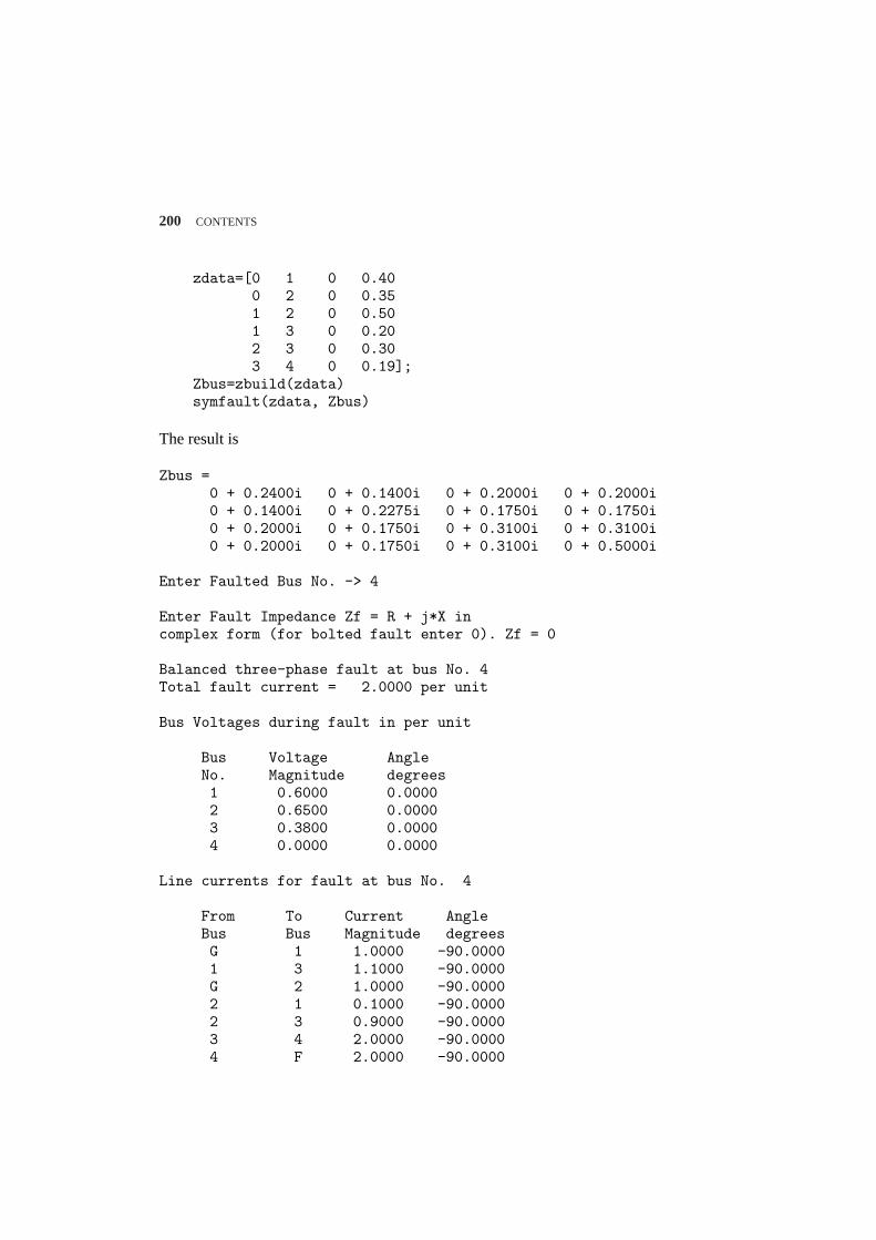
200 CONTENTS
zdata=[0 1 0 0.400 2 0 0.351 2 0 0.501 3 0 0.202 3 0 0.303 4 0 0.19];
Zbus=zbuild(zdata)symfault(zdata, Zbus)
The result is
Zbus =0 + 0.2400i 0 + 0.1400i 0 + 0.2000i 0 + 0.2000i0 + 0.1400i 0 + 0.2275i 0 + 0.1750i 0 + 0.1750i0 + 0.2000i 0 + 0.1750i 0 + 0.3100i 0 + 0.3100i0 + 0.2000i 0 + 0.1750i 0 + 0.3100i 0 + 0.5000i
Enter Faulted Bus No. -> 4
Enter Fault Impedance Zf = R + j*X incomplex form (for bolted fault enter 0). Zf = 0
Balanced three-phase fault at bus No. 4Total fault current = 2.0000 per unit
Bus Voltages during fault in per unit
Bus Voltage AngleNo. Magnitude degrees1 0.6000 0.00002 0.6500 0.00003 0.3800 0.00004 0.0000 0.0000
Line currents for fault at bus No. 4
From To Current AngleBus Bus Magnitude degreesG 1 1.0000 -90.00001 3 1.1000 -90.0000G 2 1.0000 -90.00002 1 0.1000 -90.00002 3 0.9000 -90.00003 4 2.0000 -90.00004 F 2.0000 -90.0000
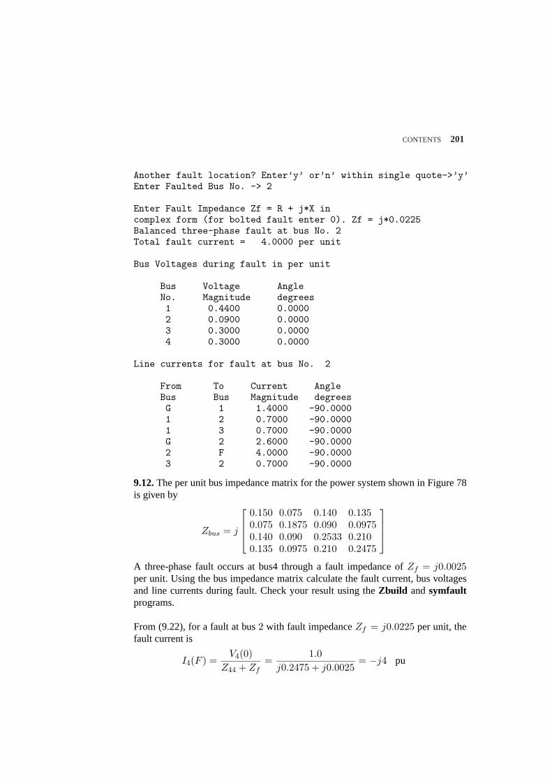
CONTENTS 201
Another fault location? Enter’y’ or’n’ within single quote->’y’Enter Faulted Bus No. -> 2
Enter Fault Impedance Zf = R + j*X incomplex form (for bolted fault enter 0). Zf = j*0.0225Balanced three-phase fault at bus No. 2Total fault current = 4.0000 per unit
Bus Voltages during fault in per unit
Bus Voltage AngleNo. Magnitude degrees1 0.4400 0.00002 0.0900 0.00003 0.3000 0.00004 0.3000 0.0000
Line currents for fault at bus No. 2
From To Current AngleBus Bus Magnitude degreesG 1 1.4000 -90.00001 2 0.7000 -90.00001 3 0.7000 -90.0000G 2 2.6000 -90.00002 F 4.0000 -90.00003 2 0.7000 -90.0000
9.12.The per unit bus impedance matrix for the power system shown in Figure 78is given by
Zbus = j
0.150 0.075 0.140 0.1350.075 0.1875 0.090 0.09750.140 0.090 0.2533 0.2100.135 0.0975 0.210 0.2475
A three-phase fault occurs at bus4 through a fault impedance ofZf = j0.0025per unit. Using the bus impedance matrix calculate the fault current, bus voltagesand line currents during fault. Check your result using theZbuild andsymfaultprograms.
From (9.22), for a fault at bus2 with fault impedanceZf = j0.0225 per unit, thefault current is
I4(F ) =V4(0)
Z44 + Zf=
1.0j0.2475 + j0.0025
= −j4 pu
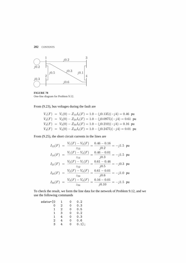
202 CONTENTS
µ´¶³
µ´¶³
....................................................................................................................................................
....................................................................................................................................................
.............................................................................................................................................................................................................................................................................................................................................................................
1
2
3
4
j0.2
j0.3
j0.2
j0.6
j0.5 j0.1j0.3
FIGURE 78One-line diagram for Problem 9.12.
From (9.23), bus voltages during the fault are
V1(F ) = V1(0)− Z14I4(F ) = 1.0− (j0.135)(−j4) = 0.46 pu
V2(F ) = V2(0)− Z24I4(F ) = 1.0− (j0.0975)(−j4) = 0.61 pu
V3(F ) = V3(0)− Z34I4(F ) = 1.0− (j0.210)(−j4) = 0.16 pu
V4(F ) = V4(0)− Z44I4(F ) = 1.0− (j0.2475)(−j4) = 0.01 pu
From (9.25), the short circuit currents in the lines are
I13(F ) =V1(F )− V3(F )
z13=
0.46− 0.16j0.2
= −j1.5 pu
I14(F ) =V1(F )− V4(F )
z14=
0.46− 0.01j0.3
= −j1.5 pu
I21(F ) =V2(F )− V1(F )
z12=
0.61− 0.46j0.5
= −j0.3 pu
I24(F ) =V2(F )− V4(F )
z24=
0.61− 0.01j0.6
= −j1.0 pu
I34(F ) =V3(F )− V4(F )
z34=
0.16− 0.01j0.10
= −j1.5 pu
To check the result, we form the line data for the network of Problem 9.12, and weuse the following commands
zdata=[0 1 0 0.20 2 0 0.31 2 0 0.51 3 0 0.21 4 0 0.32 4 0 0.63 4 0 0.1];
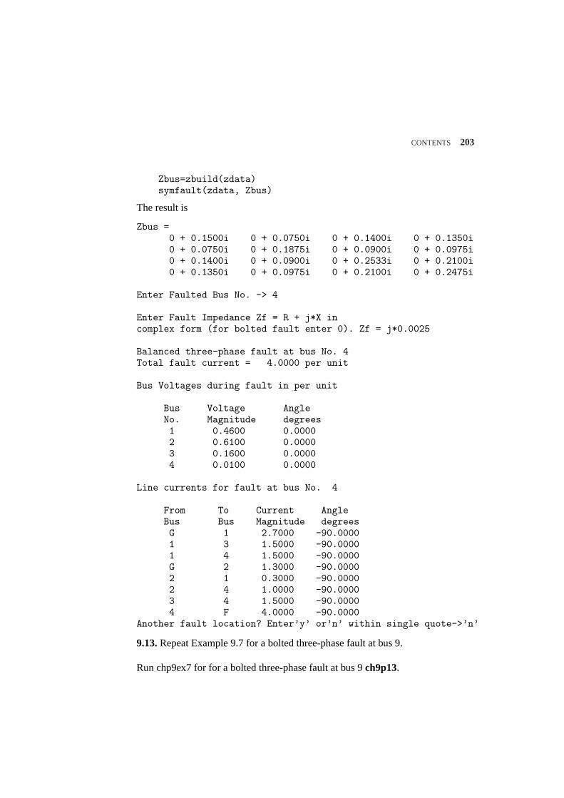
CONTENTS 203
Zbus=zbuild(zdata)symfault(zdata, Zbus)
The result is
Zbus =0 + 0.1500i 0 + 0.0750i 0 + 0.1400i 0 + 0.1350i0 + 0.0750i 0 + 0.1875i 0 + 0.0900i 0 + 0.0975i0 + 0.1400i 0 + 0.0900i 0 + 0.2533i 0 + 0.2100i0 + 0.1350i 0 + 0.0975i 0 + 0.2100i 0 + 0.2475i
Enter Faulted Bus No. -> 4
Enter Fault Impedance Zf = R + j*X incomplex form (for bolted fault enter 0). Zf = j*0.0025
Balanced three-phase fault at bus No. 4Total fault current = 4.0000 per unit
Bus Voltages during fault in per unit
Bus Voltage AngleNo. Magnitude degrees1 0.4600 0.00002 0.6100 0.00003 0.1600 0.00004 0.0100 0.0000
Line currents for fault at bus No. 4
From To Current AngleBus Bus Magnitude degreesG 1 2.7000 -90.00001 3 1.5000 -90.00001 4 1.5000 -90.0000G 2 1.3000 -90.00002 1 0.3000 -90.00002 4 1.0000 -90.00003 4 1.5000 -90.00004 F 4.0000 -90.0000
Another fault location? Enter’y’ or’n’ within single quote->’n’
9.13.Repeat Example 9.7 for a bolted three-phase fault at bus 9.
Run chp9ex7 for for a bolted three-phase fault at bus 9ch9p13.
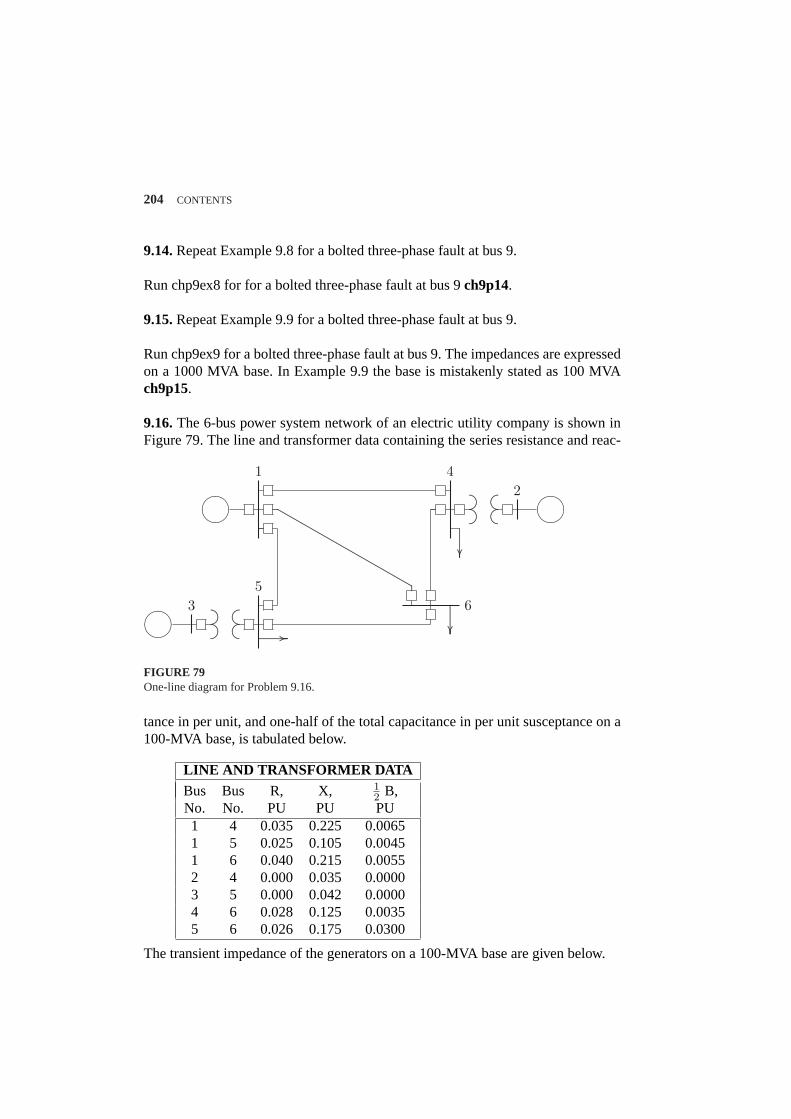
204 CONTENTS
9.14.Repeat Example 9.8 for a bolted three-phase fault at bus 9.
Run chp9ex8 for for a bolted three-phase fault at bus 9ch9p14.
9.15.Repeat Example 9.9 for a bolted three-phase fault at bus 9.
Run chp9ex9 for a bolted three-phase fault at bus 9. The impedances are expressedon a 1000 MVA base. In Example 9.9 the base is mistakenly stated as 100 MVAch9p15.
9.16.The 6-bus power system network of an electric utility company is shown inFigure 79. The line and transformer data containing the series resistance and reac-
µ´¶³
...................................................................................... ...................................................................................... µ´
¶³........................................................................................................................................................................................................................................................................................................................
µ´¶³
...................................................................................... ......................................................................................
...............................................................
........
........
........
....................................................................... ................
...............................................................
........
........
........
12
3
4
56
FIGURE 79One-line diagram for Problem 9.16.
tance in per unit, and one-half of the total capacitance in per unit susceptance on a100-MVA base, is tabulated below.
LINE AND TRANSFORMER DATABus Bus R, X, 1
2 B,No. No. PU PU PU1 4 0.035 0.225 0.00651 5 0.025 0.105 0.00451 6 0.040 0.215 0.00552 4 0.000 0.035 0.00003 5 0.000 0.042 0.00004 6 0.028 0.125 0.00355 6 0.026 0.175 0.0300
The transient impedance of the generators on a 100-MVA base are given below.
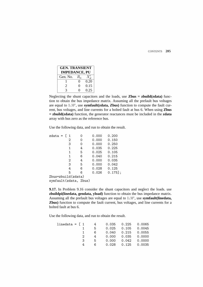
CONTENTS 205
GEN. TRANSIENTIMPEDANCE, PU
Gen. No. Ra X ′d
1 0 0.202 0 0.153 0 0.25
Neglecting the shunt capacitors and the loads, useZbus = zbuild(zdata) func-tion to obtain the bus impedance matrix. Assuming all the prefault bus voltagesare equal to16 0, usesymfault(zdata, Zbus) function to compute the fault cur-rent, bus voltages, and line currents for a bolted fault at bus 6. When usingZbus= zbuild(zdata) function, the generator reactances must be included in thezdataarray with bus zero as the reference bus.
Use the following data, and run to obtain the result.
zdata = [ 1 0 0.000 0.2002 0 0.000 0.1503 0 0.000 0.2501 4 0.035 0.2251 5 0.025 0.1051 6 0.040 0.2152 4 0.000 0.0353 5 0.000 0.0424 6 0.028 0.1255 6 0.026 0.175];
Zbus=zbuild(zdata)symfault(zdata, Zbus)
9.17. In Problem 9.16 consider the shunt capacitors and neglect the loads. usezbuildpi(linedata, gendata, yload)function to obtain the bus impedance matrix.Assuming all the prefault bus voltages are equal to1 6 0, usesymfault(linedata,Zbus) function to compute the fault current, bus voltages, and line currents for abolted fault at bus 6.
Use the following data, and run to obtain the result.
linedata = [ 1 4 0.035 0.225 0.00651 5 0.025 0.105 0.00451 6 0.040 0.215 0.00552 4 0.000 0.035 0.00003 5 0.000 0.042 0.00004 6 0.028 0.125 0.0035
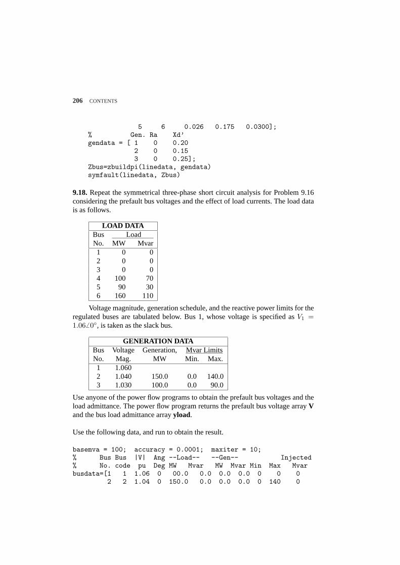
206 CONTENTS
5 6 0.026 0.175 0.0300];% Gen. Ra Xd’gendata = [ 1 0 0.20
2 0 0.153 0 0.25];
Zbus=zbuildpi(linedata, gendata)symfault(linedata, Zbus)
9.18.Repeat the symmetrical three-phase short circuit analysis for Problem 9.16considering the prefault bus voltages and the effect of load currents. The load datais as follows.
LOAD DATABus LoadNo. MW Mvar1 0 02 0 03 0 04 100 705 90 306 160 110
Voltage magnitude, generation schedule, and the reactive power limits for theregulated buses are tabulated below. Bus 1, whose voltage is specified asV1 =1.066 0, is taken as the slack bus.
GENERATION DATABus Voltage Generation, Mvar LimitsNo. Mag. MW Min. Max.1 1.0602 1.040 150.0 0.0 140.03 1.030 100.0 0.0 90.0
Use anyone of the power flow programs to obtain the prefault bus voltages and theload admittance. The power flow program returns the prefault bus voltage arrayVand the bus load admittance arrayyload.
Use the following data, and run to obtain the result.
basemva = 100; accuracy = 0.0001; maxiter = 10;% Bus Bus |V| Ang --Load-- --Gen-- Injected% No. code pu Deg MW Mvar MW Mvar Min Max Mvarbusdata=[1 1 1.06 0 00.0 0.0 0.0 0.0 0 0 0
2 2 1.04 0 150.0 0.0 0.0 0.0 0 140 0
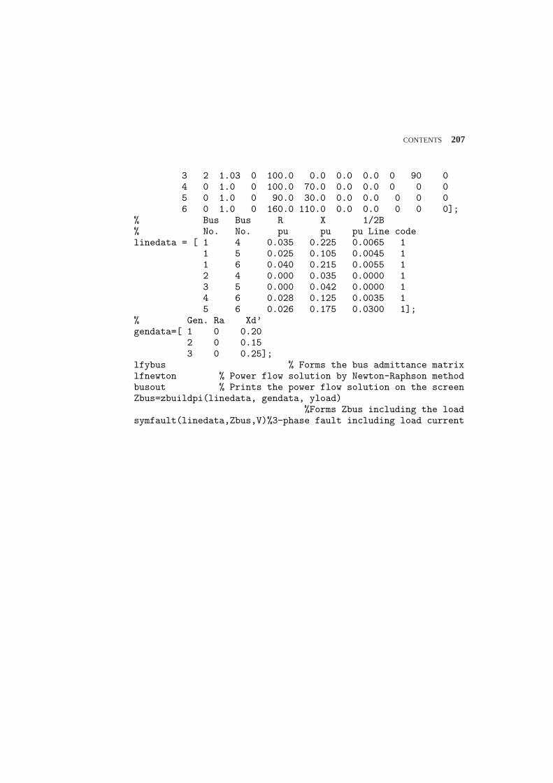
CONTENTS 207
3 2 1.03 0 100.0 0.0 0.0 0.0 0 90 04 0 1.0 0 100.0 70.0 0.0 0.0 0 0 05 0 1.0 0 90.0 30.0 0.0 0.0 0 0 06 0 1.0 0 160.0 110.0 0.0 0.0 0 0 0];
% Bus Bus R X 1/2B% No. No. pu pu pu Line codelinedata = [ 1 4 0.035 0.225 0.0065 1
1 5 0.025 0.105 0.0045 11 6 0.040 0.215 0.0055 12 4 0.000 0.035 0.0000 13 5 0.000 0.042 0.0000 14 6 0.028 0.125 0.0035 15 6 0.026 0.175 0.0300 1];
% Gen. Ra Xd’gendata=[ 1 0 0.20
2 0 0.153 0 0.25];
lfybus % Forms the bus admittance matrixlfnewton % Power flow solution by Newton-Raphson methodbusout % Prints the power flow solution on the screenZbus=zbuildpi(linedata, gendata, yload)
%Forms Zbus including the loadsymfault(linedata,Zbus,V)%3-phase fault including load current
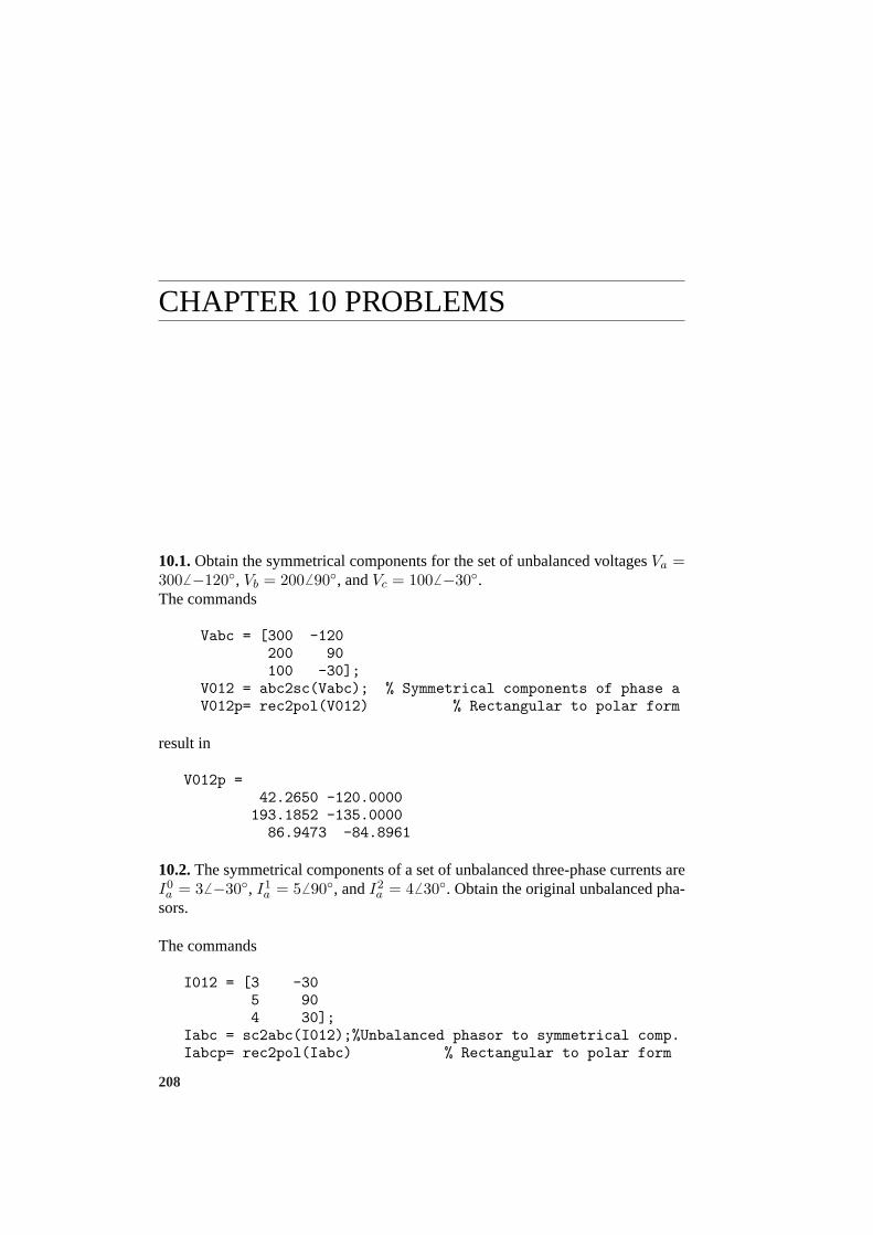
CHAPTER 10 PROBLEMS
10.1.Obtain the symmetrical components for the set of unbalanced voltagesVa =3006 −120, Vb = 2006 90, andVc = 1006 −30.The commands
Vabc = [300 -120200 90100 -30];
V012 = abc2sc(Vabc); % Symmetrical components of phase aV012p= rec2pol(V012) % Rectangular to polar form
result in
V012p =42.2650 -120.0000
193.1852 -135.000086.9473 -84.8961
10.2.The symmetrical components of a set of unbalanced three-phase currents areI0a = 36 −30, I1
a = 56 90, andI2a = 46 30. Obtain the original unbalanced pha-
sors.
The commands
I012 = [3 -305 904 30];
Iabc = sc2abc(I012);%Unbalanced phasor to symmetrical comp.Iabcp= rec2pol(Iabc) % Rectangular to polar form
208
CONTENTS 209
result in
Iabcp =8.1854 42.21634.0000 -30.00008.1854 -102.2163
10.3.The operatora is defined asa = 1 6 120; show that(a) (1+a)
(1+a2)= 1 6 120
(b) (1−a)2
(1+a)2= 3 6 −180
(c) (a− a2)(a2 − a) = 36 0(d) V 1
an = 1√3V 1
bc6 90
(e)V 2an = 1√
3V 2
bc6 −90
(a) Since1 + a + a2 = 0, we have
(1 + a)(1 + a2)
=1 + a
−a= −1
a− 1
= 0.5 + j0.866− 1 = 16 120
(b)
(1− a)2
(1 + a)2=
(1− a)2
(−a2)2=
1− 2a + a2
a=
1a− 2 + a =
= −0.5− j0.866− 2− 0.5 + j0.866 = 36 180
(c)
(a− a2)(a2 − a) = 2a3 − a2 − a4 = 2a3 − (a2 + a)= 2(1)− (−1) = 3
(d)
V 1bc = V 1
bn − V 1cn = a2V 1
an − aV 1an = (a2 − a)V 1
an
= (−0.5− j0.866 + 0.5− j0.866)V 1an
=√
36 −90V 1an
or
V 1an =
1√3V 1
bc6 90
210 CONTENTS
(e)
V 2bc = V 2
bn − V 2cn = aV 2
an − a2V 2an = (a− a2)V 2
an
= (−0.5 + j0.866 + 0.5 + j0.866)V 2an
=√
36 90V 2an
or
V 2an =
1√3V 2
bc6 −90
10.4. The line-to-line voltages in an unbalanced three-phase supply areVab =10006 0, Vbc = 866.02546 −150, andVca = 5006 120. Determine the sym-metrical components for line and phase voltages, then find the phase voltagesVan,Vbn, andVcn.
First find the symmetrical components of line voltages, then find the symmetricalcomponents of phase voltages. Use the inverse symmetrical components transfor-mation to obtain the phase voltages. We use the following commands
a = -0.5+j*sqrt(3)/2;Vabbcca=[1000 0 % Unbalanced line-to-line voltage
866.0254 -150500 120];
VL012=abc2sc(Vabbcca); % Sym. comp. line voltages, rectangularVL012p=rec2pol(VL012) % Sym. comp. line voltages, polarVa012=[ 0 % Sym. comp. phase voltages, rectangular
VL012(2)/(sqrt(3)*(0.866+j0.5))VL012(3)/(sqrt(3)*(0.866-j0.5))];
Va012p=rec2pol(Va012) % Sym. comp. phase voltage, polarVabc=sc2abc(Va012); % Unbalanced phase voltages, rectangularVabcp=rec2pol(Vabc) % Unbalanced phase voltages, polar
The result is
VL012p =0.0000 30.0000
763.7626 -10.8934288.6751 30.0000
Va012p =0 0
440.9586 -40.8934166.6667 60.0000
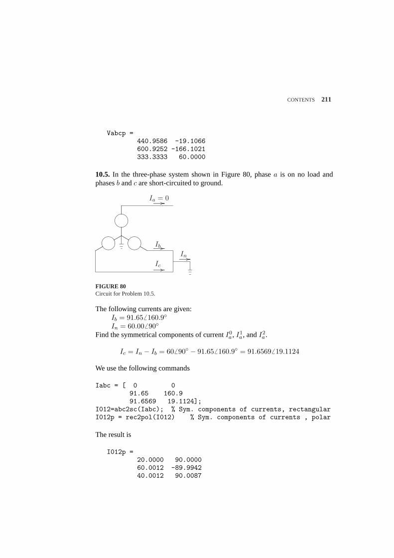
CONTENTS 211
Vabcp =440.9586 -19.1066600.9252 -166.1021333.3333 60.0000
10.5. In the three-phase system shown in Figure 80, phasea is on no load andphasesb andc are short-circuited to ground.
........
........
........
........
.µ´¶³........
........
........
........
.
.................................
µ´¶³.................................
.................................
µ´¶³
.................................Ib......................................................... ................
Ia = 0......................................................... ................
In......................................................... ................
Ic......................................................... ................
FIGURE 80Circuit for Problem 10.5.
The following currents are given:Ib = 91.656 160.9In = 60.006 90
Find the symmetrical components of currentI0a , I1
a , andI2a .
Ic = In − Ib = 60 6 90 − 91.656 160.9 = 91.65696 19.1124
We use the following commands
Iabc = [ 0 091.65 160.991.6569 19.1124];
I012=abc2sc(Iabc); % Sym. components of currents, rectangularI012p = rec2pol(I012) % Sym. components of currents , polar
The result is
I012p =20.0000 90.000060.0012 -89.994240.0012 90.0087
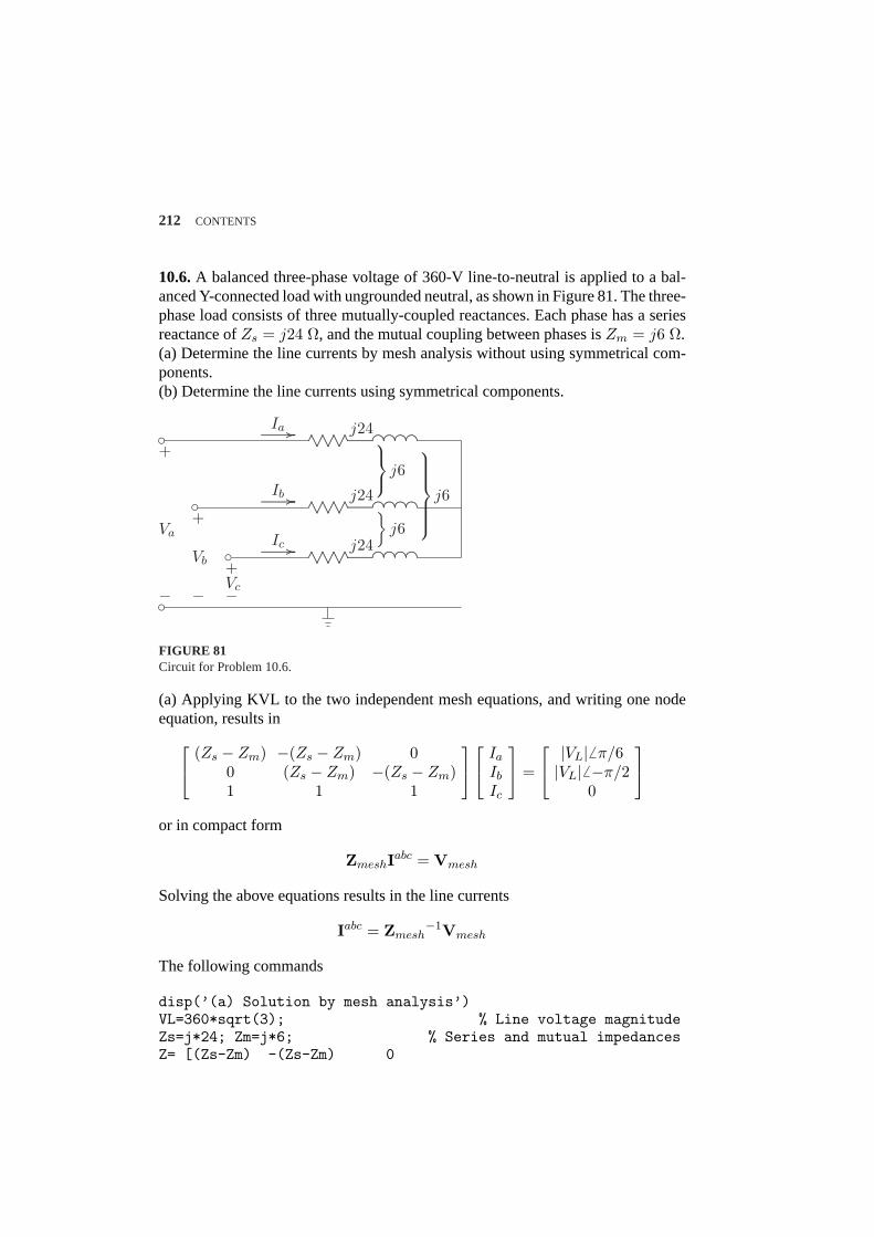
212 CONTENTS
10.6.A balanced three-phase voltage of 360-V line-to-neutral is applied to a bal-anced Y-connected load with ungrounded neutral, as shown in Figure 81. The three-phase load consists of three mutually-coupled reactances. Each phase has a seriesreactance ofZs = j24 Ω, and the mutual coupling between phases isZm = j6 Ω.(a) Determine the line currents by mesh analysis without using symmetrical com-ponents.(b) Determine the line currents using symmetrical components.
c ..........................................
............................................
............................................
................................................................... .........
..................... .............................. .........
..................... ..............................
......................................................................... ................Ia j24
c ..........................................
............................................
............................................
................................................................... .........
..................... .............................. .........
..................... ..............................
......................................................................... ................Ib j24
c ..........................................
............................................
............................................
................................................................... .........
..................... .............................. .........
..................... ..............................
......................................................................... ................Ic j24
c
Va
+
−
Vb
+
− Vc
+
−
j6
j6
j6
FIGURE 81Circuit for Problem 10.6.
(a) Applying KVL to the two independent mesh equations, and writing one nodeequation, results in
(Zs − Zm) −(Zs − Zm) 00 (Zs − Zm) −(Zs − Zm)1 1 1
Ia
Ib
Ic
=
|VL|6 π/6|VL|6 −π/2
0
or in compact form
ZmeshIabc = Vmesh
Solving the above equations results in the line currents
Iabc = Zmesh−1Vmesh
The following commands
disp(’(a) Solution by mesh analysis’)VL=360*sqrt(3); % Line voltage magnitudeZs=j*24; Zm=j*6; % Series and mutual impedancesZ= [(Zs-Zm) -(Zs-Zm) 0
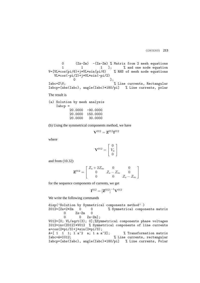
CONTENTS 213
0 (Zs-Zm) -(Zs-Zm) % Matrix from 2 mesh equations1 1 1 ]; % and one node equation
V=[VL*cos(pi/6)+j*VL*sin(pi/6) % RHS of mesh node equationsVL*cos(-pi/2)+j*VL*sin(-pi/2)
0 ];Iabc=Z\V; % Line currents, RectangularIabcp=[abs(Iabc), angle(Iabc)*180/pi] % Line currents, polar
The result is
(a) Solution by mesh analysisIabcp =
20.0000 -90.000020.0000 150.000020.0000 30.0000
(b) Using the symmetrical components method, we have
V012 = Z012I012
where
V012 =
0Va
0
and from (10.32)
Z012 =
Zs + 2Zm 0 00 Zs − Zm 00 0 Zs − Zm
for the sequence components of currents, we get
I012 = [Z012]−1V012
We write the following commands
disp(’Solution by Symmetrical components method’ )Z012=[Zs+2*Zm 0 0 % Symmetrical components matrix
0 Zs-Zm 00 0 Zs-Zm];
V012=[0; VL/sqrt(3); 0];%Symmetrical components phase voltagesI012=inv(Z012)*V012 % Symmetrical components of line currentsa=cos(2*pi/3)+j*sin(2*pi/3);A=[ 1 1 1; 1 a^2 a; 1 a a^2]; % Transformation matrixIabc=A*I012; % Line currents, rectangularIabcp=[abs(Iabc), angle(Iabc)*180/pi] % Line currents, Polar
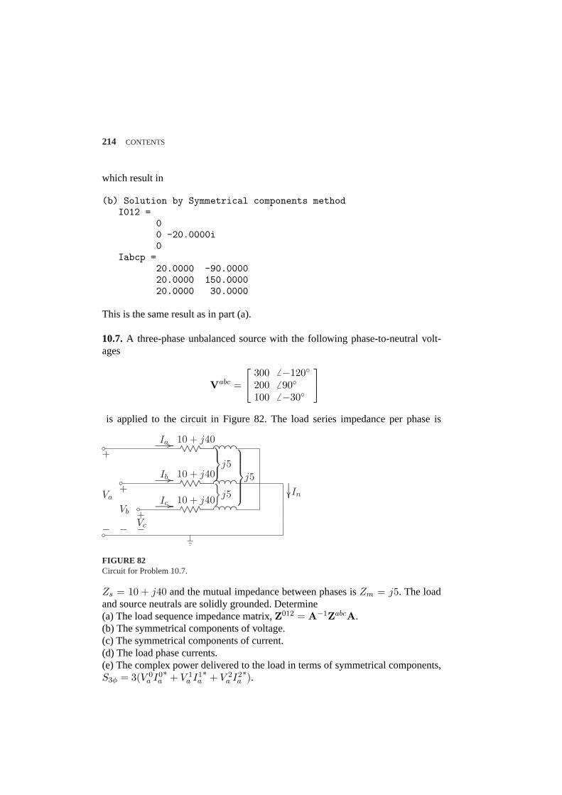
214 CONTENTS
which result in
(b) Solution by Symmetrical components methodI012 =
00 -20.0000i0
Iabcp =20.0000 -90.000020.0000 150.000020.0000 30.0000
This is the same result as in part (a).
10.7.A three-phase unbalanced source with the following phase-to-neutral volt-ages
Vabc =
300 6 −120200 6 90100 6 −30
is applied to the circuit in Figure 82. The load series impedance per phase is
b ........................................................................
......................................................................................... ...........
.............. ......................... ...........
.............. ........................................................................................ ................
Ia 10 + j40
b ........................................................................
......................................................................................... ...........
.............. ......................... ...........
.............. ........................................................................................ ................
Ib 10 + j40
b ........................................................................
......................................................................................... ...........
.............. ......................... ...........
.............. ........................................................................................ ................
Ic 10 + j40
b
...............................................
........
........
........InVa
+
−Vb
+
− Vc
+−
j5
j5
j5
FIGURE 82Circuit for Problem 10.7.
Zs = 10 + j40 and the mutual impedance between phases isZm = j5. The loadand source neutrals are solidly grounded. Determine(a) The load sequence impedance matrix,Z012 = A−1ZabcA.(b) The symmetrical components of voltage.(c) The symmetrical components of current.(d) The load phase currents.(e) The complex power delivered to the load in terms of symmetrical components,S3φ = 3(V 0
a I0a∗ + V 1
a I1a∗ + V 2
a I2a∗).
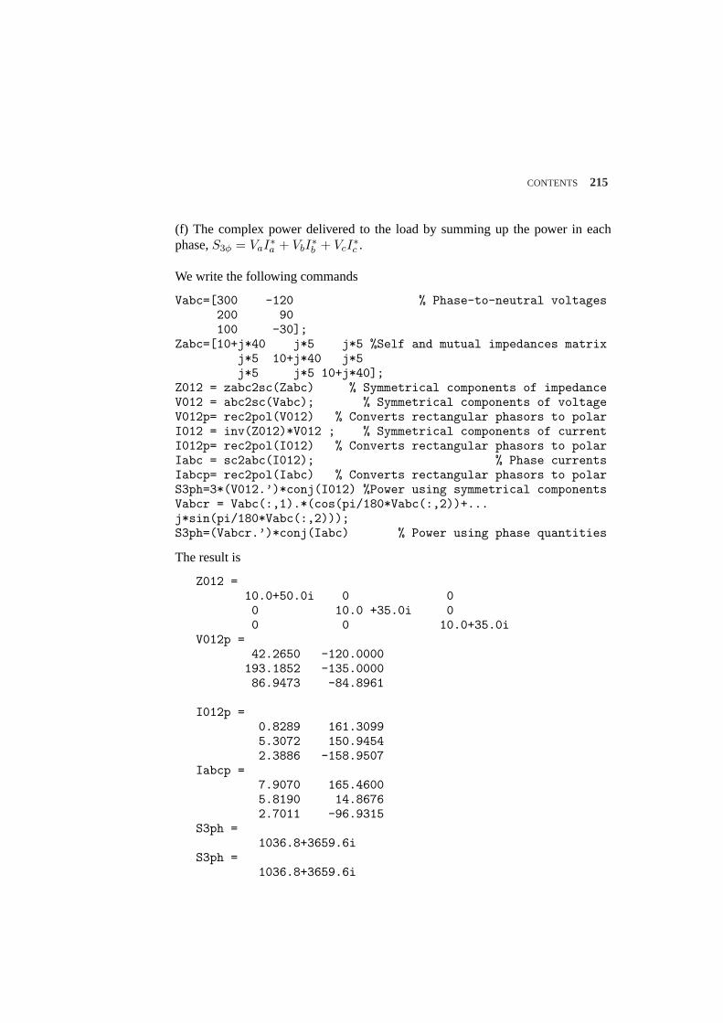
CONTENTS 215
(f) The complex power delivered to the load by summing up the power in eachphase,S3φ = VaI
∗a + VbI
∗b + VcI
∗c .
We write the following commands
Vabc=[300 -120 % Phase-to-neutral voltages200 90100 -30];
Zabc=[10+j*40 j*5 j*5 %Self and mutual impedances matrixj*5 10+j*40 j*5j*5 j*5 10+j*40];
Z012 = zabc2sc(Zabc) % Symmetrical components of impedanceV012 = abc2sc(Vabc); % Symmetrical components of voltageV012p= rec2pol(V012) % Converts rectangular phasors to polarI012 = inv(Z012)*V012 ; % Symmetrical components of currentI012p= rec2pol(I012) % Converts rectangular phasors to polarIabc = sc2abc(I012); % Phase currentsIabcp= rec2pol(Iabc) % Converts rectangular phasors to polarS3ph=3*(V012.’)*conj(I012) %Power using symmetrical componentsVabcr = Vabc(:,1).*(cos(pi/180*Vabc(:,2))+...j*sin(pi/180*Vabc(:,2)));S3ph=(Vabcr.’)*conj(Iabc) % Power using phase quantities
The result is
Z012 =10.0+50.0i 0 00 10.0 +35.0i 00 0 10.0+35.0i
V012p =42.2650 -120.0000193.1852 -135.000086.9473 -84.8961
I012p =0.8289 161.30995.3072 150.94542.3886 -158.9507
Iabcp =7.9070 165.46005.8190 14.86762.7011 -96.9315
S3ph =1036.8+3659.6i
S3ph =1036.8+3659.6i
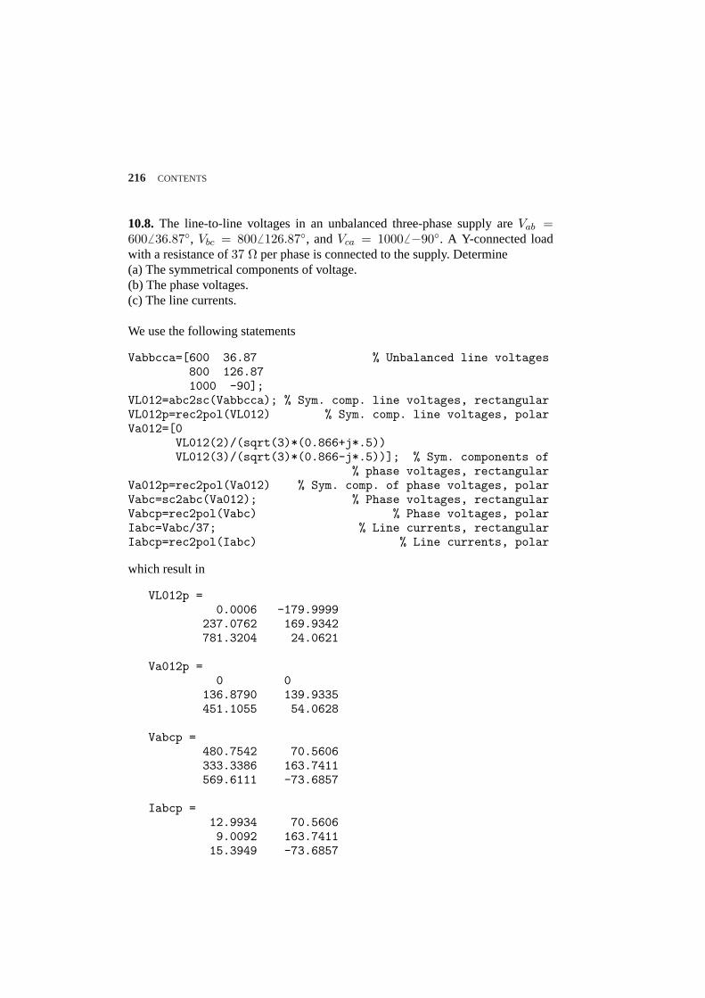
216 CONTENTS
10.8. The line-to-line voltages in an unbalanced three-phase supply areVab =6006 36.87, Vbc = 8006 126.87, andVca = 10006 −90. A Y-connected loadwith a resistance of37 Ω per phase is connected to the supply. Determine(a) The symmetrical components of voltage.(b) The phase voltages.(c) The line currents.
We use the following statements
Vabbcca=[600 36.87 % Unbalanced line voltages800 126.871000 -90];
VL012=abc2sc(Vabbcca); % Sym. comp. line voltages, rectangularVL012p=rec2pol(VL012) % Sym. comp. line voltages, polarVa012=[0
VL012(2)/(sqrt(3)*(0.866+j*.5))VL012(3)/(sqrt(3)*(0.866-j*.5))]; % Sym. components of
% phase voltages, rectangularVa012p=rec2pol(Va012) % Sym. comp. of phase voltages, polarVabc=sc2abc(Va012); % Phase voltages, rectangularVabcp=rec2pol(Vabc) % Phase voltages, polarIabc=Vabc/37; % Line currents, rectangularIabcp=rec2pol(Iabc) % Line currents, polar
which result in
VL012p =0.0006 -179.9999
237.0762 169.9342781.3204 24.0621
Va012p =0 0
136.8790 139.9335451.1055 54.0628
Vabcp =480.7542 70.5606333.3386 163.7411569.6111 -73.6857
Iabcp =12.9934 70.56069.0092 163.741115.3949 -73.6857
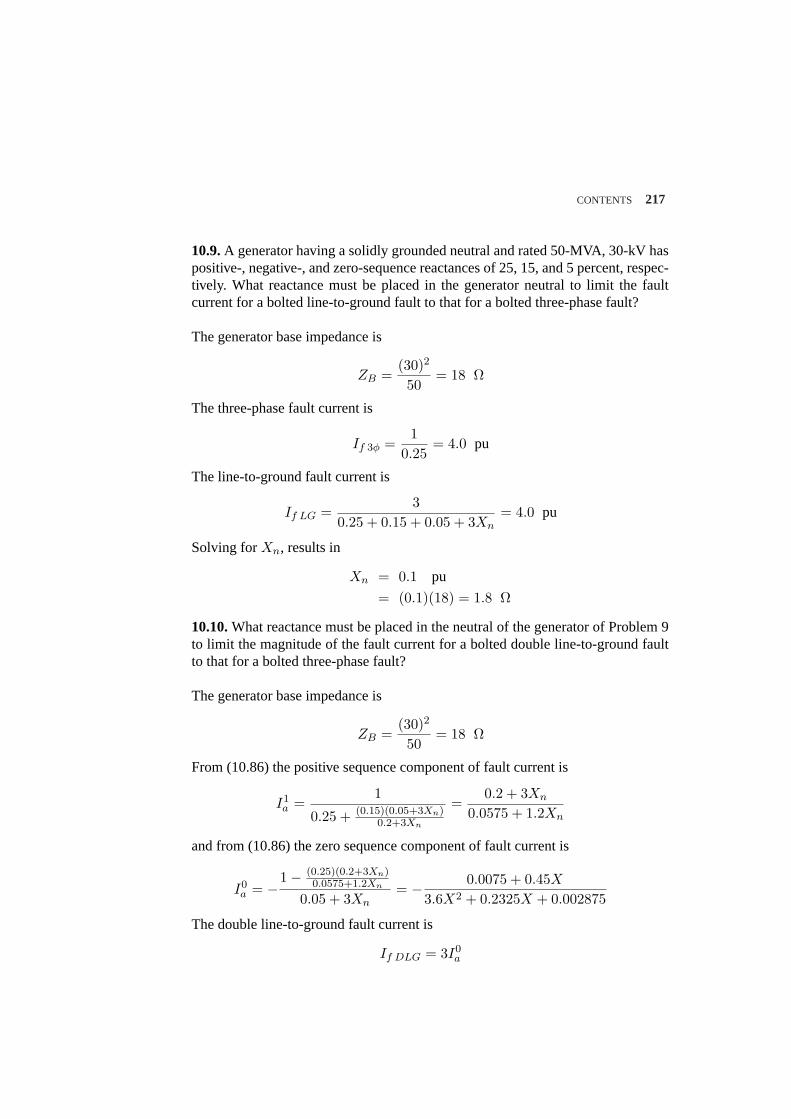
CONTENTS 217
10.9.A generator having a solidly grounded neutral and rated 50-MVA, 30-kV haspositive-, negative-, and zero-sequence reactances of 25, 15, and 5 percent, respec-tively. What reactance must be placed in the generator neutral to limit the faultcurrent for a bolted line-to-ground fault to that for a bolted three-phase fault?
The generator base impedance is
ZB =(30)2
50= 18 Ω
The three-phase fault current is
If 3φ =1
0.25= 4.0 pu
The line-to-ground fault current is
If LG =3
0.25 + 0.15 + 0.05 + 3Xn= 4.0 pu
Solving forXn, results in
Xn = 0.1 pu
= (0.1)(18) = 1.8 Ω
10.10.What reactance must be placed in the neutral of the generator of Problem 9to limit the magnitude of the fault current for a bolted double line-to-ground faultto that for a bolted three-phase fault?
The generator base impedance is
ZB =(30)2
50= 18 Ω
From (10.86) the positive sequence component of fault current is
I1a =
1
0.25 + (0.15)(0.05+3Xn)0.2+3Xn
=0.2 + 3Xn
0.0575 + 1.2Xn
and from (10.86) the zero sequence component of fault current is
I0a = −1− (0.25)(0.2+3Xn)
0.0575+1.2Xn
0.05 + 3Xn= − 0.0075 + 0.45X
3.6X2 + 0.2325X + 0.002875
The double line-to-ground fault current is
If DLG = 3I0a
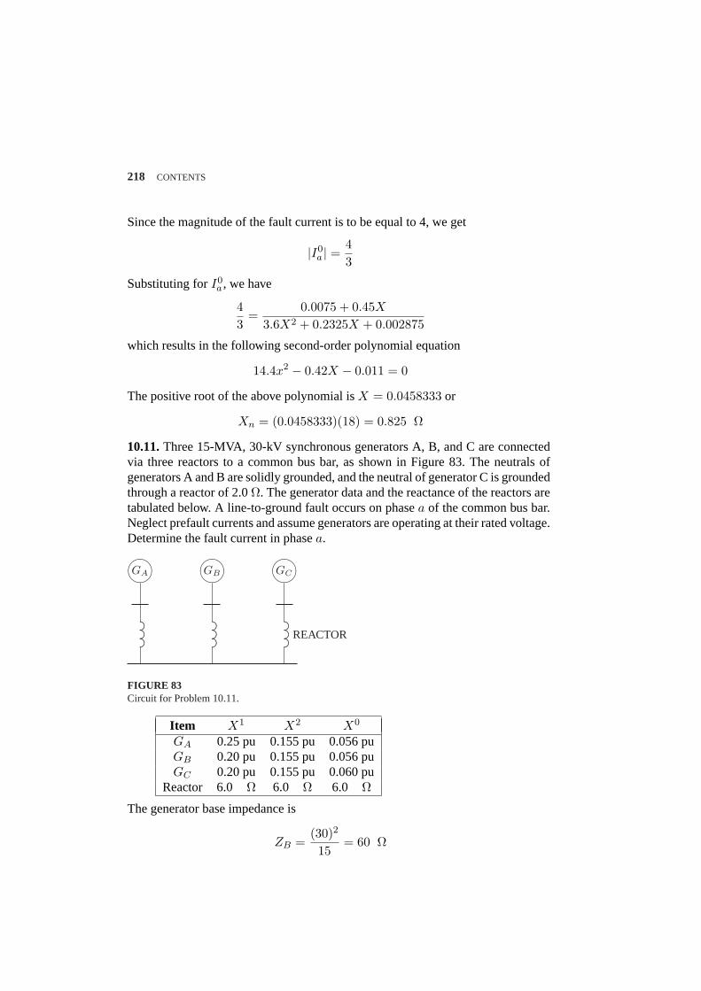
218 CONTENTS
Since the magnitude of the fault current is to be equal to 4, we get
|I0a | =
43
Substituting forI0a , we have
43
=0.0075 + 0.45X
3.6X2 + 0.2325X + 0.002875
which results in the following second-order polynomial equation
14.4x2 − 0.42X − 0.011 = 0
The positive root of the above polynomial isX = 0.0458333 or
Xn = (0.0458333)(18) = 0.825 Ω
10.11.Three 15-MVA, 30-kV synchronous generators A, B, and C are connectedvia three reactors to a common bus bar, as shown in Figure 83. The neutrals ofgenerators A and B are solidly grounded, and the neutral of generator C is groundedthrough a reactor of 2.0Ω. The generator data and the reactance of the reactors aretabulated below. A line-to-ground fault occurs on phasea of the common bus bar.Neglect prefault currents and assume generators are operating at their rated voltage.Determine the fault current in phasea.
µ´¶³GA
.......................................................................................
µ´¶³GB
.......................................................................................
µ´¶³GC
.......................................................................................
REACTOR
FIGURE 83Circuit for Problem 10.11.
Item X1 X2 X0
GA 0.25 pu 0.155 pu 0.056 puGB 0.20 pu 0.155 pu 0.056 puGC 0.20 pu 0.155 pu 0.060 pu
Reactor 6.0 Ω 6.0 Ω 6.0 Ω
The generator base impedance is
ZB =(30)2
15= 60 Ω
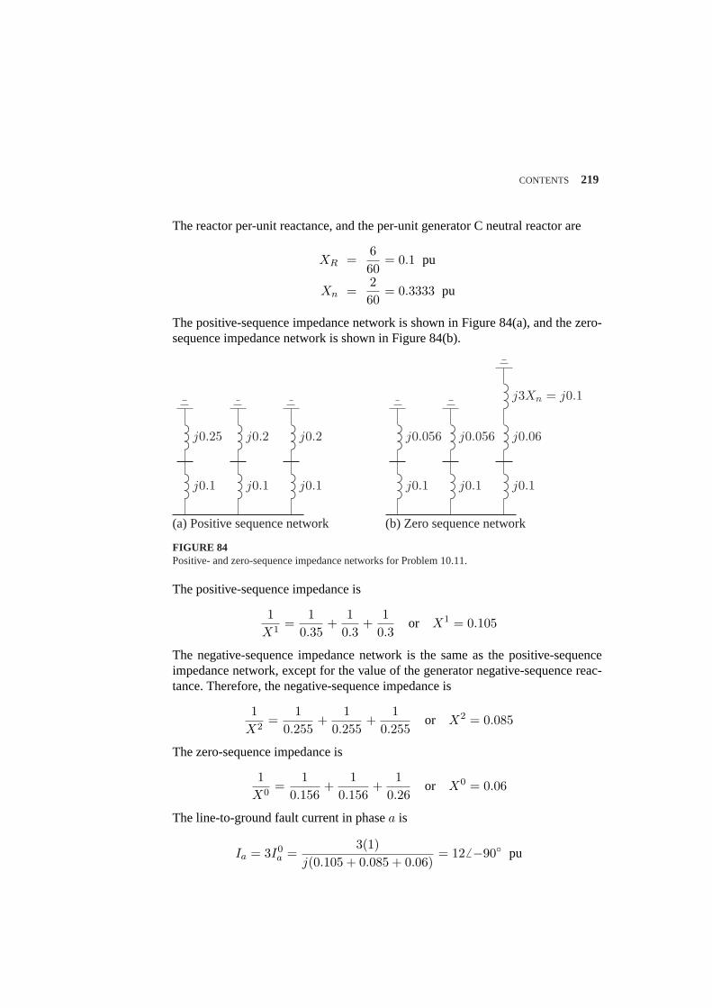
CONTENTS 219
The reactor per-unit reactance, and the per-unit generator C neutral reactor are
XR =660
= 0.1 pu
Xn =260
= 0.3333 pu
The positive-sequence impedance network is shown in Figure 84(a), and the zero-sequence impedance network is shown in Figure 84(b).
.................................................................................
.................................................................................
j0.25
j0.1
.................................................................................
.................................................................................
j0.2
j0.1
.................................................................................
j0.2
j0.1.................................................................................
.................................................................................
.................................................................................
j0.056
j0.1
.................................................................................
.................................................................................
j0.056
j0.1
...........................
...........................
........................... j3Xn = j0.1
.................................................................................
j0.06
j0.1.................................................................................
(a) Positive sequence network (b) Zero sequence network
FIGURE 84Positive- and zero-sequence impedance networks for Problem 10.11.
The positive-sequence impedance is
1X1
=1
0.35+
10.3
+1
0.3or X1 = 0.105
The negative-sequence impedance network is the same as the positive-sequenceimpedance network, except for the value of the generator negative-sequence reac-tance. Therefore, the negative-sequence impedance is
1X2
=1
0.255+
10.255
+1
0.255or X2 = 0.085
The zero-sequence impedance is
1X0
=1
0.156+
10.156
+1
0.26or X0 = 0.06
The line-to-ground fault current in phasea is
Ia = 3I0a =
3(1)j(0.105 + 0.085 + 0.06)
= 12 6 −90 pu
220 CONTENTS
10.12.Repeat Problem 10.11 for a bolted line-to-line fault between phasesb andc.
The positive-sequence fault current in phasea is
I1a =
1Z1 + Z2
=1
j(0.105 + 0.085)= −j5.26316 pu
The fault current is
Ib = −j√
3I1a = −9.116 pu
10.13.Repeat Problem 10.11 for a bolted double line-to-ground fault on phasesbandc.
The positive- and zero-sequence fault currents in phasea are
I1a =
1
j0.105 + j(
(0.085)(0.06)0.085+0.06
) = −j7.13407 pu
I0a = −1− (j0.105)(−j7.13407)
j0.06= j4.182 pu
The fault current is
If = 3I0a = 12.5466 90
10.14.The zero-, positive-, and negative-sequence bus impedance matrices for athree-bus power system are
Z0bus = j
0.20 0.05 0.120.05 0.10 0.080.12 0.08 0.30
pu
Z1bus = Z2
bus = j
0.16 0.10 0.150.10 0.20 0.120.15 0.12 0.25
pu
Determine the per unit fault current and the bus voltages during fault for(a) A bolted three-phase fault at bus 2.(b) A bolted single line-to-ground fault at bus 2.(c) A bolted line-to-line fault at bus 2.(d) A bolted double line-to-ground fault at bus 2.
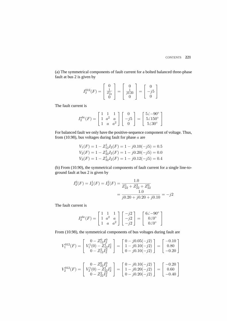
CONTENTS 221
(a) The symmetrical components of fault current for a bolted balanced three-phasefault at bus 2 is given by
I0122 (F ) =
01
Z122
0
=
01
j0.20
0
=
0−j50
The fault current is
Iabc2 (F ) =
1 1 11 a2 a1 a a2
0−j50
=
56 −9056 1505 6 30
For balanced fault we only have the positive-sequence component of voltage. Thus,from (10.98), bus voltages during fault for phasea are
V1(F ) = 1− Z112I2(F ) = 1− j0.10(−j5) = 0.5
V2(F ) = 1− Z122I2(F ) = 1− j0.20(−j5) = 0.0
V3(F ) = 1− Z132I2(F ) = 1− j0.12(−j5) = 0.4
(b) From (10.90), the symmetrical components of fault current for a single line-to-ground fault at bus 2 is given by
I02 (F ) = I1
2 (F ) = I22 (F ) =
1.0Z1
22 + Z222 + Z0
22
=1.0
j0.20 + j0.20 + j0.10= −j2
The fault current is
Iabc2 (F ) =
1 1 11 a2 a1 a a2
−j2−j2−j2
=
66 −9006 006 0
From (10.98), the symmetrical components of bus voltages during fault are
V 0121 (F ) =
0− Z012I
02
V 11 (0)− Z1
12I12
0− Z212I
22
=
0− j0.05(−j2)1− j0.10(−j2)0− j0.10(−j2)
=
−0.100.80−0.20
V 0122 (F ) =
0− Z022I
02
V 12 (0)− Z1
22I12
0− Z222I
22
=
0− j0.10(−j2)1− j0.20(−j2)0− j0.20(−j2)
=
−0.200.60−0.40
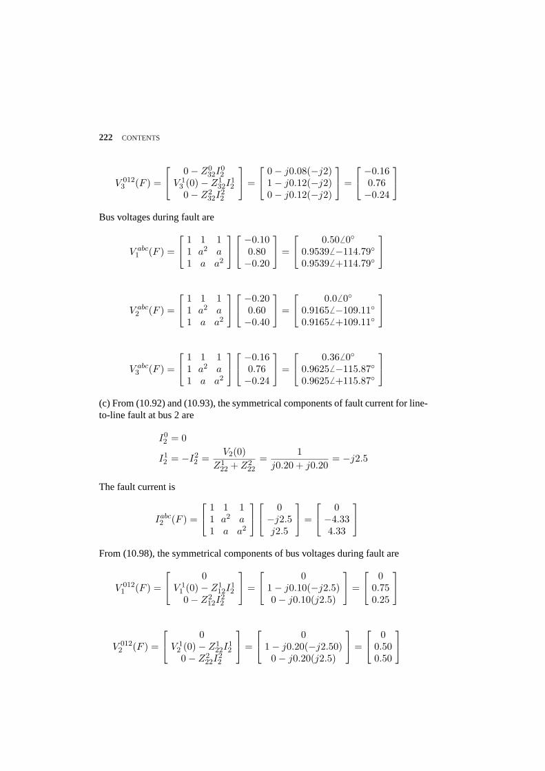
222 CONTENTS
V 0123 (F ) =
0− Z032I
02
V 13 (0)− Z1
32I12
0− Z232I
22
=
0− j0.08(−j2)1− j0.12(−j2)0− j0.12(−j2)
=
−0.160.76−0.24
Bus voltages during fault are
V abc1 (F ) =
1 1 11 a2 a1 a a2
−0.100.80−0.20
=
0.50 6 00.95396 −114.790.95396 +114.79
V abc2 (F ) =
1 1 11 a2 a1 a a2
−0.200.60−0.40
=
0.06 00.91656 −109.110.91656 +109.11
V abc3 (F ) =
1 1 11 a2 a1 a a2
−0.160.76−0.24
=
0.36 6 00.96256 −115.870.96256 +115.87
(c) From (10.92) and (10.93), the symmetrical components of fault current for line-to-line fault at bus 2 are
I02 = 0
I12 = −I2
2 =V2(0)
Z122 + Z2
22
=1
j0.20 + j0.20= −j2.5
The fault current is
Iabc2 (F ) =
1 1 11 a2 a1 a a2
0−j2.5j2.5
=
0−4.334.33
From (10.98), the symmetrical components of bus voltages during fault are
V 0121 (F ) =
0V 1
1 (0)− Z112I
12
0− Z212I
22
=
01− j0.10(−j2.5)0− j0.10(j2.5)
=
00.750.25
V 0122 (F ) =
0V 1
2 (0)− Z122I
12
0− Z222I
22
=
01− j0.20(−j2.50)0− j0.20(j2.5)
=
00.500.50
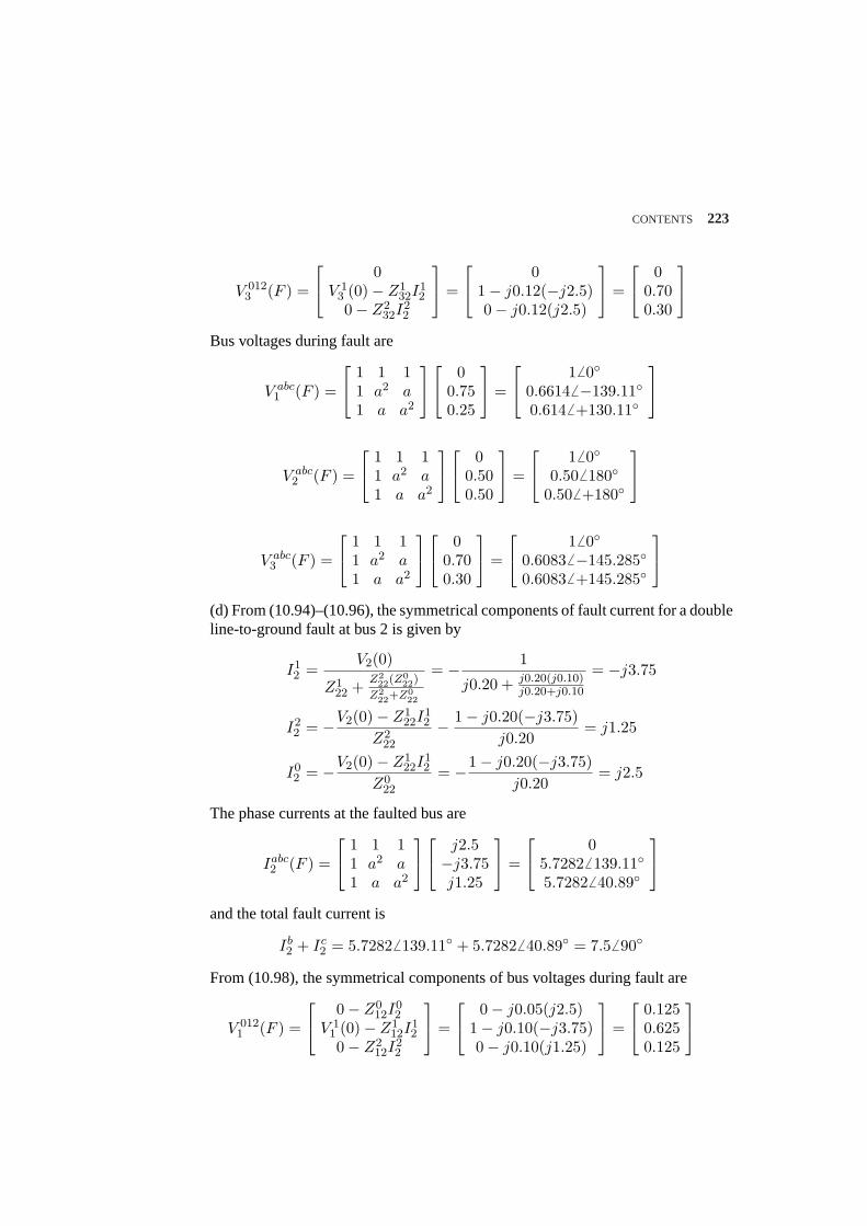
CONTENTS 223
V 0123 (F ) =
0V 1
3 (0)− Z132I
12
0− Z232I
22
=
01− j0.12(−j2.5)0− j0.12(j2.5)
=
00.700.30
Bus voltages during fault are
V abc1 (F ) =
1 1 11 a2 a1 a a2
00.750.25
=
16 00.6614 6 −139.110.6146 +130.11
V abc2 (F ) =
1 1 11 a2 a1 a a2
00.500.50
=
16 00.506 180
0.506 +180
V abc3 (F ) =
1 1 11 a2 a1 a a2
00.700.30
=
16 00.60836 −145.2850.60836 +145.285
(d) From (10.94)–(10.96), the symmetrical components of fault current for a doubleline-to-ground fault at bus 2 is given by
I12 =
V2(0)
Z122 + Z2
22(Z022)
Z222+Z0
22
= − 1
j0.20 + j0.20(j0.10)j0.20+j0.10
= −j3.75
I22 = −V2(0)− Z1
22I12
Z222
− 1− j0.20(−j3.75)j0.20
= j1.25
I02 = −V2(0)− Z1
22I12
Z022
= −1− j0.20(−j3.75)j0.20
= j2.5
The phase currents at the faulted bus are
Iabc2 (F ) =
1 1 11 a2 a1 a a2
j2.5−j3.75j1.25
=
05.72826 139.115.7282 6 40.89
and the total fault current is
Ib2 + Ic
2 = 5.72826 139.11 + 5.72826 40.89 = 7.56 90
From (10.98), the symmetrical components of bus voltages during fault are
V 0121 (F ) =
0− Z012I
02
V 11 (0)− Z1
12I12
0− Z212I
22
=
0− j0.05(j2.5)1− j0.10(−j3.75)0− j0.10(j1.25)
=
0.1250.6250.125
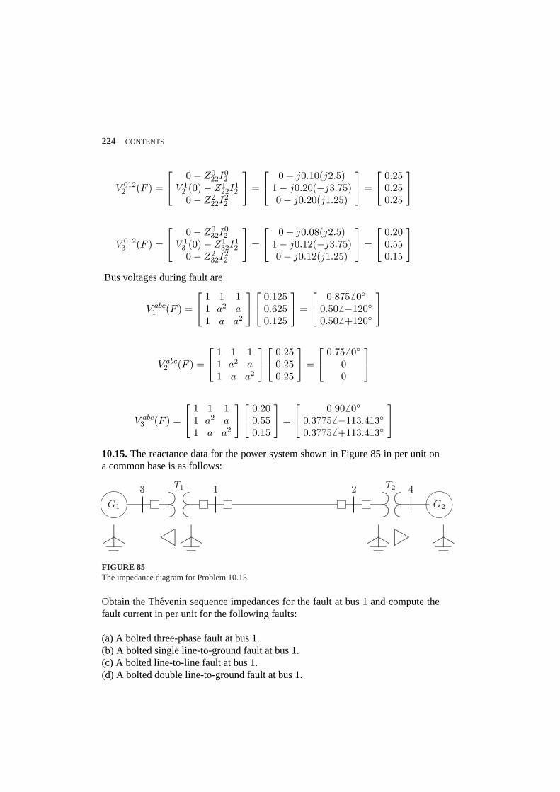
224 CONTENTS
V 0122 (F ) =
0− Z022I
02
V 12 (0)− Z1
22I12
0− Z222I
22
=
0− j0.10(j2.5)1− j0.20(−j3.75)0− j0.20(j1.25)
=
0.250.250.25
V 0123 (F ) =
0− Z032I
02
V 13 (0)− Z1
32I12
0− Z232I
22
=
0− j0.08(j2.5)1− j0.12(−j3.75)0− j0.12(j1.25)
=
0.200.550.15
Bus voltages during fault are
V abc1 (F ) =
1 1 11 a2 a1 a a2
0.1250.6250.125
=
0.8756 00.50 6 −1200.50 6 +120
V abc2 (F ) =
1 1 11 a2 a1 a a2
0.250.250.25
=
0.75 6 000
V abc3 (F ) =
1 1 11 a2 a1 a a2
0.200.550.15
=
0.90 6 00.37756 −113.4130.37756 +113.413
10.15.The reactance data for the power system shown in Figure 85 in per unit ona common base is as follows:
½¼
¾»
.............................................
....................................................
....... ........................................................................................................ .............................................
....................................................
....... ........................................................................................................ ½¼
¾»
..........................................................................
...................................................
................................
........................................................................................
............
..........................................................................
...................................................
..........................................................................
...................................................
................................................................................................
........
........
........
........
...............................................................
..............................
....................................
G1 G2
T1 T23 1 2 4
FIGURE 85The impedance diagram for Problem 10.15.
Obtain the Thevenin sequence impedances for the fault at bus 1 and compute thefault current in per unit for the following faults:
(a) A bolted three-phase fault at bus 1.(b) A bolted single line-to-ground fault at bus 1.(c) A bolted line-to-line fault at bus 1.(d) A bolted double line-to-ground fault at bus 1.
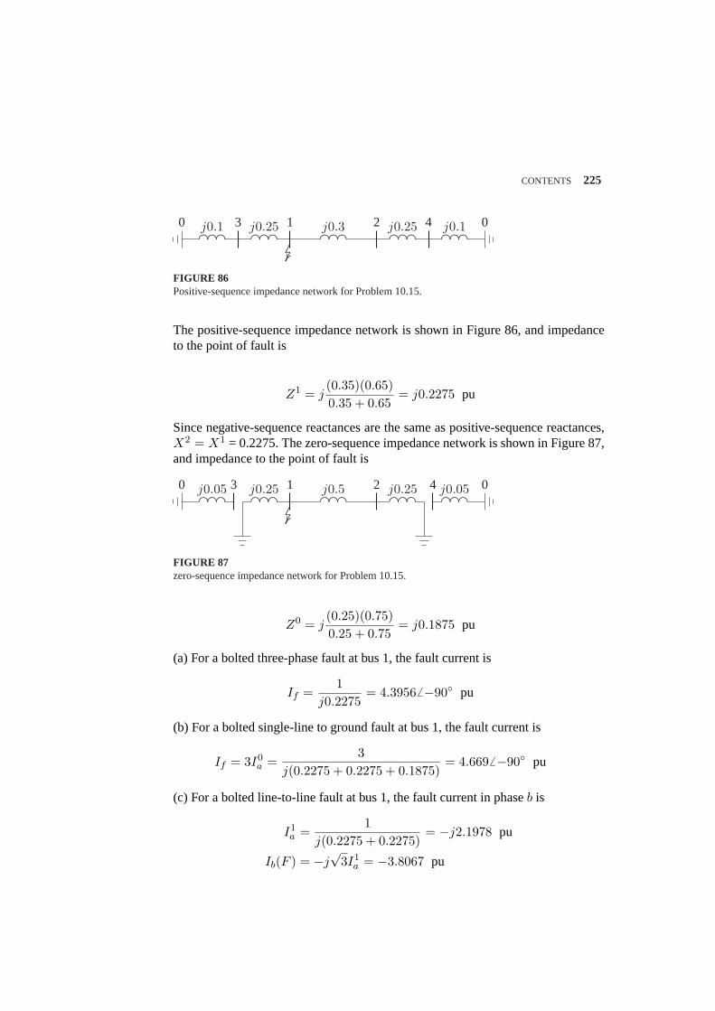
CONTENTS 225
.......................................
................................................ ..........
..........................................................
................... .......................................
................................................ ..........
..........................................................
................... .......................................
................................................
....................................................................................
j0.1 j0.25 j0.3 j0.25 j0.10 3 1 2 04
FIGURE 86Positive-sequence impedance network for Problem 10.15.
The positive-sequence impedance network is shown in Figure 86, and impedanceto the point of fault is
Z1 = j(0.35)(0.65)0.35 + 0.65
= j0.2275 pu
Since negative-sequence reactances are the same as positive-sequence reactances,X2 = X1 = 0.2275. The zero-sequence impedance network is shown in Figure 87,and impedance to the point of fault is
.......................................
................................................ ..........
..........................................................
................... .......................................
................................................ ..........
..........................................................
................... .......................................
................................................
....................................................................................
j0.05 j0.25 j0.5 j0.25 j0.050 3 1 2 04
FIGURE 87zero-sequence impedance network for Problem 10.15.
Z0 = j(0.25)(0.75)0.25 + 0.75
= j0.1875 pu
(a) For a bolted three-phase fault at bus 1, the fault current is
If =1
j0.2275= 4.39566 −90 pu
(b) For a bolted single-line to ground fault at bus 1, the fault current is
If = 3I0a =
3j(0.2275 + 0.2275 + 0.1875)
= 4.6696 −90 pu
(c) For a bolted line-to-line fault at bus 1, the fault current in phaseb is
I1a =
1j(0.2275 + 0.2275)
= −j2.1978 pu
Ib(F ) = −j√
3I1a = −3.8067 pu
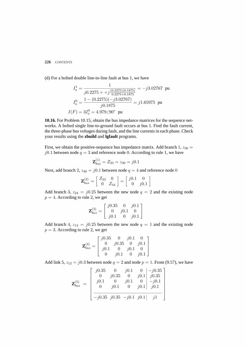
226 CONTENTS
(d) For a bolted double line-to-line fault at bus 1, we have
I1a =
1
j0.2275 + +j (0.2275)(0.1875)0.2275+0.1875
= −j3.02767 pu
I0a =
1− (0.2275)(−j3.02767)j0.1875
= j1.65975 pu
I(F ) = 3I0a = 4.9796 90 pu
10.16.For Problem 10.15, obtain the bus impedance matrices for the sequence net-works. A bolted single line-to-ground fault occurs at bus 1. Find the fault current,the three-phase bus voltages during fault, and the line currents in each phase. Checkyour results using thezbuild andlgfault programs.
First, we obtain the positive-sequence bus impedance matrix. Add branch1, z30 =j0.1 between nodeq = 3 and reference node0. According to rule 1, we have
Z(1)bus = Z33 = z30 = j0.1
Next, add branch2, z40 = j0.1 between nodeq = 4 and reference node0
Z(2)bus =
[Z33 00 Z44
]=
[j0.1 00 j0.1
]
Add branch3, z24 = j0.25 between the new nodeq = 2 and the existing nodep = 4. According to rule 2, we get
Z(3)bus =
j0.35 0 j0.10 j0.1 0
j0.1 0 j0.1
Add branch4, z13 = j0.25 between the new nodeq = 1 and the existing nodep = 3. According to rule 2, we get
Z(4)bus =
j0.35 0 j0.1 00 j0.35 0 j0.1
j0.1 0 j0.1 00 j0.1 0 j0.1
Add link 5, z12 = j0.3 between nodeq = 2 and nodep = 1. From (9.57), we have
Z(5)bus =
j0.35 0 j0.1 0 −j0.350 j0.35 0 j0.1 j0.35
j0.1 0 j0.1 0 −j0.10 j0.1 0 j0.1 j0.1
−j0.35 j0.35 −j0.1 j0.1 j1
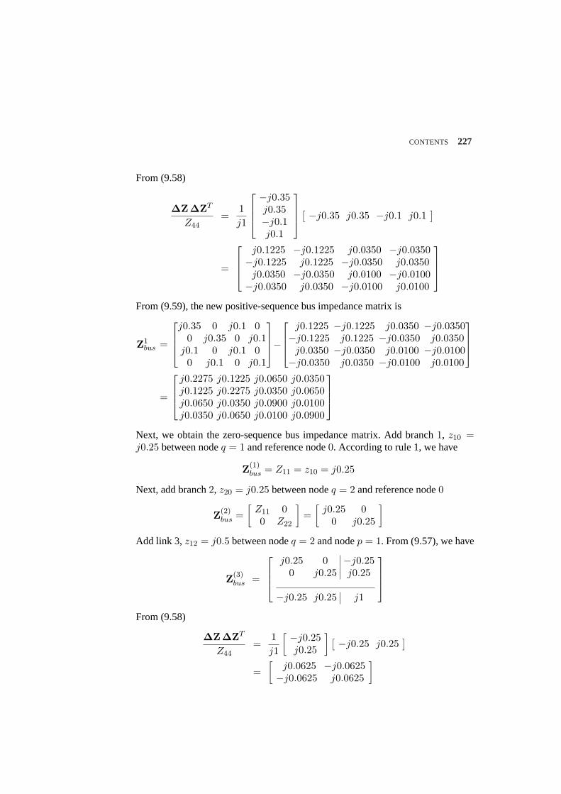
CONTENTS 227
From (9.58)
∆Z∆ZT
Z44=
1j1
−j0.35j0.35−j0.1j0.1
[ −j0.35 j0.35 −j0.1 j0.1]
=
j0.1225 −j0.1225 j0.0350 −j0.0350−j0.1225 j0.1225 −j0.0350 j0.0350
j0.0350 −j0.0350 j0.0100 −j0.0100−j0.0350 j0.0350 −j0.0100 j0.0100
From (9.59), the new positive-sequence bus impedance matrix is
Z1bus =
j0.35 0 j0.1 00 j0.35 0 j0.1
j0.1 0 j0.1 00 j0.1 0 j0.1
−
j0.1225 −j0.1225 j0.0350 −j0.0350−j0.1225 j0.1225 −j0.0350 j0.0350
j0.0350 −j0.0350 j0.0100 −j0.0100−j0.0350 j0.0350 −j0.0100 j0.0100
=
j0.2275 j0.1225 j0.0650 j0.0350j0.1225 j0.2275 j0.0350 j0.0650j0.0650 j0.0350 j0.0900 j0.0100j0.0350 j0.0650 j0.0100 j0.0900
Next, we obtain the zero-sequence bus impedance matrix. Add branch1, z10 =j0.25 between nodeq = 1 and reference node0. According to rule 1, we have
Z(1)bus = Z11 = z10 = j0.25
Next, add branch2, z20 = j0.25 between nodeq = 2 and reference node0
Z(2)bus =
[Z11 00 Z22
]=
[j0.25 0
0 j0.25
]
Add link 3, z12 = j0.5 between nodeq = 2 and nodep = 1. From (9.57), we have
Z(3)bus =
j0.25 0 −j0.250 j0.25 j0.25
−j0.25 j0.25 j1
From (9.58)
∆Z∆ZT
Z44=
1j1
[ −j0.25j0.25
] [ −j0.25 j0.25]
=[
j0.0625 −j0.0625−j0.0625 j0.0625
]
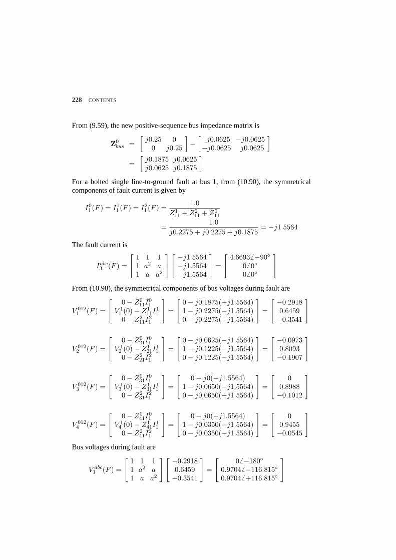
228 CONTENTS
From (9.59), the new positive-sequence bus impedance matrix is
Z0bus =
[j0.25 0
0 j0.25
]−
[j0.0625 −j0.0625−j0.0625 j0.0625
]
=[
j0.1875 j0.0625j0.0625 j0.1875
]
For a bolted single line-to-ground fault at bus 1, from (10.90), the symmetricalcomponents of fault current is given by
I01 (F ) = I1
1 (F ) = I21 (F ) =
1.0Z1
11 + Z211 + Z0
11
=1.0
j0.2275 + j0.2275 + j0.1875= −j1.5564
The fault current is
Iabc3 (F ) =
1 1 11 a2 a1 a a2
−j1.5564−j1.5564−j1.5564
=
4.6693 6 −9006 006 0
From (10.98), the symmetrical components of bus voltages during fault are
V 0121 (F ) =
0− Z011I
01
V 11 (0)− Z1
11I11
0− Z211I
21
=
0− j0.1875(−j1.5564)1− j0.2275(−j1.5564)0− j0.2275(−j1.5564)
=
−0.29180.6459−0.3541
V 0122 (F ) =
0− Z021I
01
V 12 (0)− Z1
21I11
0− Z221I
21
=
0− j0.0625(−j1.5564)1− j0.1225(−j1.5564)0− j0.1225(−j1.5564)
=
−0.09730.8093−0.1907
V 0123 (F ) =
0− Z031I
01
V 13 (0)− Z1
31I11
0− Z231I
21
=
0− j0(−j1.5564)1− j0.0650(−j1.5564)0− j0.0650(−j1.5564)
=
00.8988−0.1012
V 0124 (F ) =
0− Z041I
01
V 14 (0)− Z1
41I11
0− Z241I
21
=
0− j0(−j1.5564)1− j0.0350(−j1.5564)0− j0.0350(−j1.5564)
=
00.9455−0.0545
Bus voltages during fault are
V abc1 (F ) =
1 1 11 a2 a1 a a2
−0.29180.6459−0.3541
=
06 −1800.97046 −116.8150.97046 +116.815
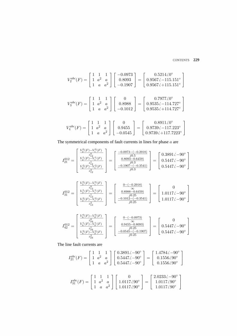
CONTENTS 229
V abc2 (F ) =
1 1 11 a2 a1 a a2
−0.09730.8093−0.1907
=
0.52146 00.95676 −115.1510.95676 +115.151
V abc3 (F ) =
1 1 11 a2 a1 a a2
00.8988−0.1012
=
0.79776 00.95356 −114.7270.95356 +114.727
V abc4 (F ) =
1 1 11 a2 a1 a a2
00.9455−0.0545
=
0.89116 00.97396 −117.2230.97396 +117.7223
The symmetrical components of fault currents in lines for phasea are
I01221 =
V 02 (F )−V 0
1 (F )
z012
V 12 (F )−V 1
1 (F )
z112
V 22 (F )−V 2
1 (F )
z212
=
−0.0973−(−0.2918)j0.5
0.8093−0.6459)j0.3
−0.1907−(−0.3541)j0.3
=
0.38916 −90
0.54476 −90
0.54476 −90
I01231 =
V 03 (F )−V 0
1 (F )
z013
V 13 (F )−V 1
1 (F )
z113
V 23 (F )−V 2
1 (F )
z213
=
0−(−0.2918)∞
0.8988−0.6459)j0.25
−0.1012−(−0.3541)j0.25
=
01.01176 −90
1.01176 −90
I01242 =
V 04 (F )−V 0
2 (F )
z024
V 14 (F )−V 1
2 (F )
z124
V 24 (F )−V 2
2 (F )
z224
=
0−(−0.0973)∞
0.9455−0.8093)j0.25
−0.0545−(−0.1907)j0.25
=
00.54476 −90
0.54476 −90
The line fault currents are
Iabc21 (F ) =
1 1 11 a2 a1 a a2
0.38916 −900.54476 −900.54476 −90
=
1.47846 −900.15566 900.15566 90
Iabc31 (F ) =
1 1 11 a2 a1 a a2
01.01176 901.01176 90
=
2.02336 −901.01176 901.01176 90
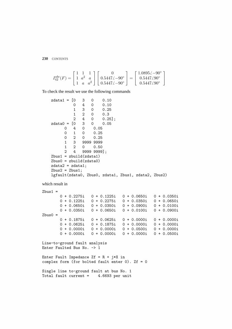
230 CONTENTS
Iabc42 (F ) =
1 1 11 a2 a1 a a2
00.54476 −900.54476 −90
=
1.08956 −900.54476 900.54476 90
To check the result we use the following commands
zdata1 = [0 3 0 0.100 4 0 0.101 3 0 0.251 2 0 0.32 4 0 0.25];
zdata0 = [0 3 0 0.050 4 0 0.050 1 0 0.250 2 0 0.251 3 9999 99991 2 0 0.502 4 9999 9999];
Zbus1 = zbuild(zdata1)Zbus0 = zbuild(zdata0)zdata2 = zdata1;Zbus2 = Zbus1;lgfault(zdata0, Zbus0, zdata1, Zbus1, zdata2, Zbus2)
which result in
Zbus1 =0 + 0.2275i 0 + 0.1225i 0 + 0.0650i 0 + 0.0350i0 + 0.1225i 0 + 0.2275i 0 + 0.0350i 0 + 0.0650i0 + 0.0650i 0 + 0.0350i 0 + 0.0900i 0 + 0.0100i0 + 0.0350i 0 + 0.0650i 0 + 0.0100i 0 + 0.0900i
Zbus0 =0 + 0.1875i 0 + 0.0625i 0 + 0.0000i 0 + 0.0000i0 + 0.0625i 0 + 0.1875i 0 + 0.0000i 0 + 0.0000i0 + 0.0000i 0 + 0.0000i 0 + 0.0500i 0 + 0.0000i0 + 0.0000i 0 + 0.0000i 0 + 0.0000i 0 + 0.0500i
Line-to-ground fault analysisEnter Faulted Bus No. -> 1
Enter Fault Impedance Zf = R + j*X incomplex form (for bolted fault enter 0). Zf = 0
Single line to-ground fault at bus No. 1Total fault current = 4.6693 per unit
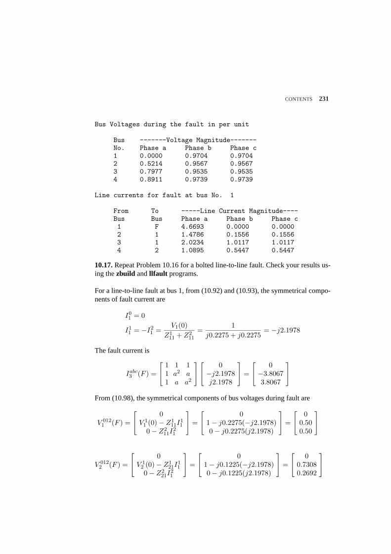
CONTENTS 231
Bus Voltages during the fault in per unit
Bus -------Voltage Magnitude-------No. Phase a Phase b Phase c1 0.0000 0.9704 0.97042 0.5214 0.9567 0.95673 0.7977 0.9535 0.95354 0.8911 0.9739 0.9739
Line currents for fault at bus No. 1
From To -----Line Current Magnitude----Bus Bus Phase a Phase b Phase c1 F 4.6693 0.0000 0.00002 1 1.4786 0.1556 0.15563 1 2.0234 1.0117 1.01174 2 1.0895 0.5447 0.5447
10.17.Repeat Problem 10.16 for a bolted line-to-line fault. Check your results us-ing thezbuild andllfault programs.
For a line-to-line fault at bus 1, from (10.92) and (10.93), the symmetrical compo-nents of fault current are
I01 = 0
I11 = −I2
1 =V1(0)
Z111 + Z2
11
=1
j0.2275 + j0.2275= −j2.1978
The fault current is
Iabc3 (F ) =
1 1 11 a2 a1 a a2
0−j2.1978j2.1978
=
0−3.80673.8067
From (10.98), the symmetrical components of bus voltages during fault are
V 0121 (F ) =
0V 1
1 (0)− Z111I
11
0− Z211I
21
=
01− j0.2275(−j2.1978)0− j0.2275(j2.1978)
=
00.500.50
V 0122 (F ) =
0V 1
2 (0)− Z121I
11
0− Z221I
21
=
01− j0.1225(−j2.1978)0− j0.1225(j2.1978)
=
00.73080.2692
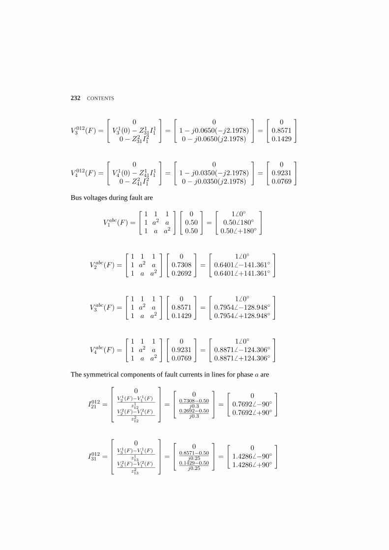
232 CONTENTS
V 0123 (F ) =
0V 1
3 (0)− Z131I
11
0− Z231I
21
=
01− j0.0650(−j2.1978)0− j0.0650(j2.1978)
=
00.85710.1429
V 0124 (F ) =
0V 1
4 (0)− Z141I
11
0− Z241I
21
=
01− j0.0350(−j2.1978)0− j0.0350(j2.1978)
=
00.92310.0769
Bus voltages during fault are
V abc1 (F ) =
1 1 11 a2 a1 a a2
00.500.50
=
16 00.506 180
0.506 +180
V abc2 (F ) =
1 1 11 a2 a1 a a2
00.73080.2692
=
16 00.64016 −141.3610.64016 +141.361
V abc3 (F ) =
1 1 11 a2 a1 a a2
00.85710.1429
=
16 00.79546 −128.9480.79546 +128.948
V abc4 (F ) =
1 1 11 a2 a1 a a2
00.92310.0769
=
16 00.88716 −124.3060.88716 +124.306
The symmetrical components of fault currents in lines for phasea are
I01221 =
0V 12 (F )−V 1
1 (F )
z112
V 22 (F )−V 2
1 (F )
z212
=
00.7308−0.50
j0.30.2692−0.50
j0.3
=
00.76926 −900.76926 +90
I01231 =
0V 13 (F )−V 1
1 (F )
z113
V 23 (F )−V 2
1 (F )
z213
=
00.8571−0.50
j0.250.1429−0.50
j0.25
=
01.42866 −901.42866 +90
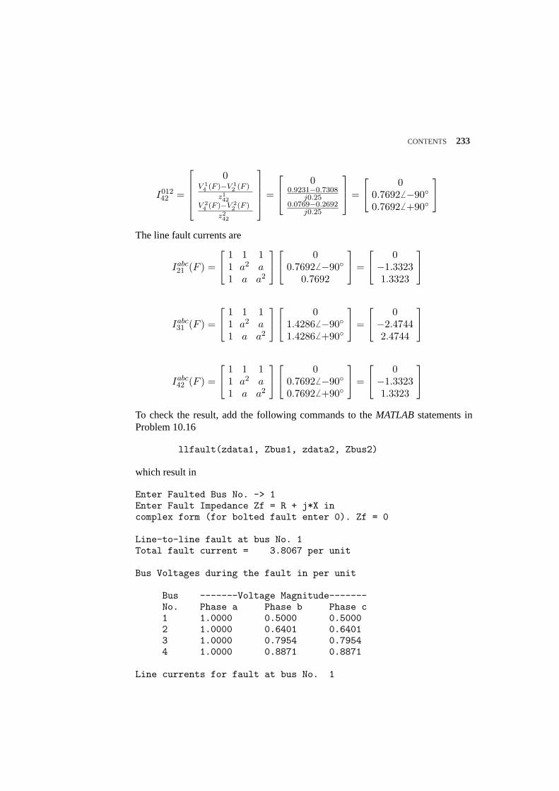
CONTENTS 233
I01242 =
0V 14 (F )−V 1
2 (F )
z142
V 24 (F )−V 2
2 (F )
z242
=
00.9231−0.7308
j0.250.0769−0.2692
j0.25
=
00.76926 −900.76926 +90
The line fault currents are
Iabc21 (F ) =
1 1 11 a2 a1 a a2
00.76926 −90
0.7692
=
0−1.33231.3323
Iabc31 (F ) =
1 1 11 a2 a1 a a2
01.42866 −901.42866 +90
=
0−2.47442.4744
Iabc42 (F ) =
1 1 11 a2 a1 a a2
00.76926 −900.76926 +90
=
0−1.33231.3323
To check the result, add the following commands to theMATLABstatements inProblem 10.16
llfault(zdata1, Zbus1, zdata2, Zbus2)
which result in
Enter Faulted Bus No. -> 1Enter Fault Impedance Zf = R + j*X incomplex form (for bolted fault enter 0). Zf = 0
Line-to-line fault at bus No. 1Total fault current = 3.8067 per unit
Bus Voltages during the fault in per unit
Bus -------Voltage Magnitude-------No. Phase a Phase b Phase c1 1.0000 0.5000 0.50002 1.0000 0.6401 0.64013 1.0000 0.7954 0.79544 1.0000 0.8871 0.8871
Line currents for fault at bus No. 1
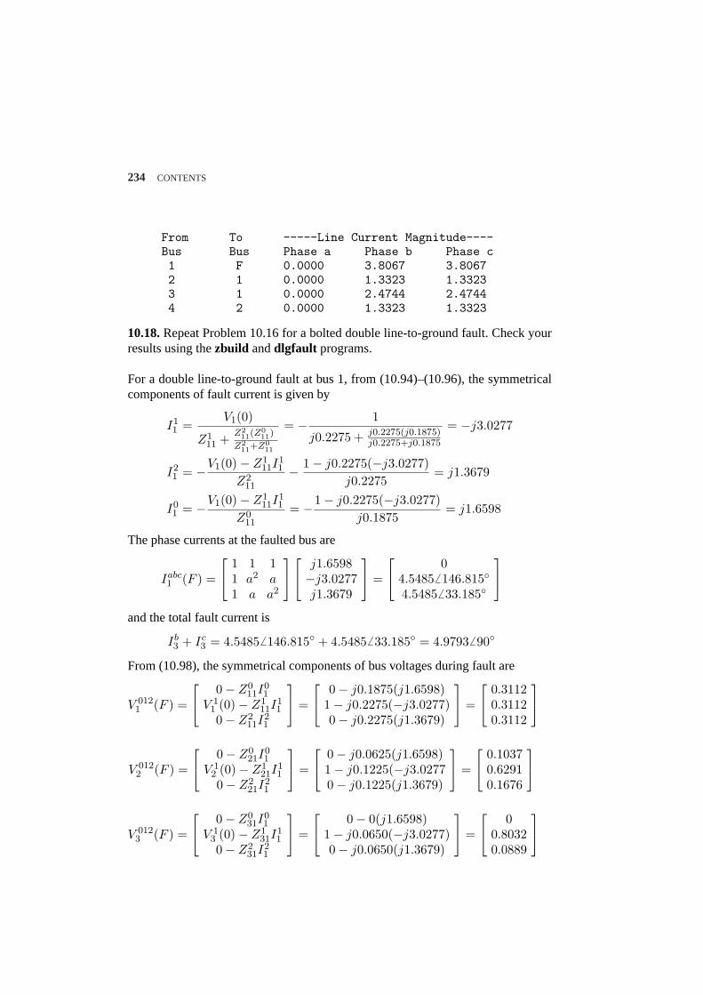
234 CONTENTS
From To -----Line Current Magnitude----Bus Bus Phase a Phase b Phase c1 F 0.0000 3.8067 3.80672 1 0.0000 1.3323 1.33233 1 0.0000 2.4744 2.47444 2 0.0000 1.3323 1.3323
10.18.Repeat Problem 10.16 for a bolted double line-to-ground fault. Check yourresults using thezbuild anddlgfault programs.
For a double line-to-ground fault at bus 1, from (10.94)–(10.96), the symmetricalcomponents of fault current is given by
I11 =
V1(0)
Z111 + Z2
11(Z011)
Z211+Z0
11
= − 1
j0.2275 + j0.2275(j0.1875)j0.2275+j0.1875
= −j3.0277
I21 = −V1(0)− Z1
11I11
Z211
− 1− j0.2275(−j3.0277)j0.2275
= j1.3679
I01 = −V1(0)− Z1
11I11
Z011
= −1− j0.2275(−j3.0277)j0.1875
= j1.6598
The phase currents at the faulted bus are
Iabc1 (F ) =
1 1 11 a2 a1 a a2
j1.6598−j3.0277j1.3679
=
04.5485 6 146.8154.54856 33.185
and the total fault current is
Ib3 + Ic
3 = 4.54856 146.815 + 4.54856 33.185 = 4.9793 6 90
From (10.98), the symmetrical components of bus voltages during fault are
V 0121 (F ) =
0− Z011I
01
V 11 (0)− Z1
11I11
0− Z211I
21
=
0− j0.1875(j1.6598)1− j0.2275(−j3.0277)0− j0.2275(j1.3679)
=
0.31120.31120.3112
V 0122 (F ) =
0− Z021I
01
V 12 (0)− Z1
21I11
0− Z221I
21
=
0− j0.0625(j1.6598)1− j0.1225(−j3.02770− j0.1225(j1.3679)
=
0.10370.62910.1676
V 0123 (F ) =
0− Z031I
01
V 13 (0)− Z1
31I11
0− Z231I
21
=
0− 0(j1.6598)1− j0.0650(−j3.0277)0− j0.0650(j1.3679)
=
00.80320.0889
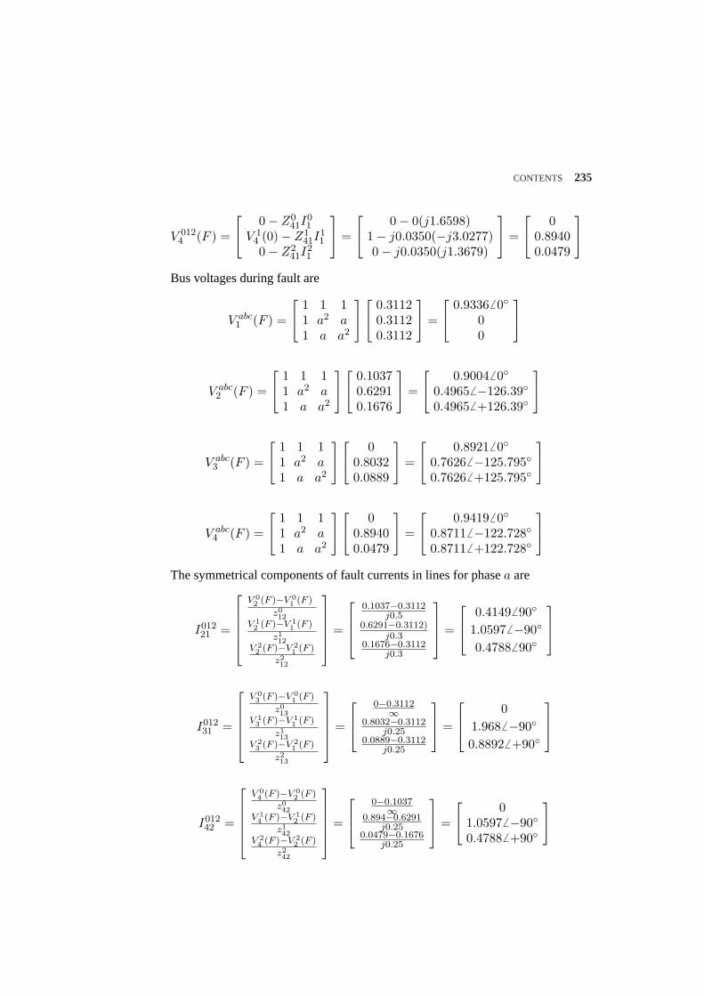
CONTENTS 235
V 0124 (F ) =
0− Z041I
01
V 14 (0)− Z1
41I11
0− Z241I
21
=
0− 0(j1.6598)1− j0.0350(−j3.0277)0− j0.0350(j1.3679)
=
00.89400.0479
Bus voltages during fault are
V abc1 (F ) =
1 1 11 a2 a1 a a2
0.31120.31120.3112
=
0.93366 000
V abc2 (F ) =
1 1 11 a2 a1 a a2
0.10370.62910.1676
=
0.90046 00.49656 −126.390.49656 +126.39
V abc3 (F ) =
1 1 11 a2 a1 a a2
00.80320.0889
=
0.89216 00.76266 −125.7950.76266 +125.795
V abc4 (F ) =
1 1 11 a2 a1 a a2
00.89400.0479
=
0.94196 00.87116 −122.7280.87116 +122.728
The symmetrical components of fault currents in lines for phasea are
I01221 =
V 02 (F )−V 0
1 (F )
z012
V 12 (F )−V 1
1 (F )
z112
V 22 (F )−V 2
1 (F )
z212
=
0.1037−0.3112j0.5
0.6291−0.3112)j0.3
0.1676−0.3112j0.3
=
0.41496 90
1.05976 −90
0.47886 90
I01231 =
V 03 (F )−V 0
1 (F )
z013
V 13 (F )−V 1
1 (F )
z113
V 23 (F )−V 2
1 (F )
z213
=
0−0.3112∞
0.8032−0.3112j0.25
0.0889−0.3112j0.25
=
01.9686 −90
0.88926 +90
I01242 =
V 04 (F )−V 0
2 (F )
z042
V 14 (F )−V 1
2 (F )
z142
V 24 (F )−V 2
2 (F )
z242
=
0−0.1037∞
0.894−0.6291j0.25
0.0479−0.1676j0.25
=
01.05976 −900.47886 +90
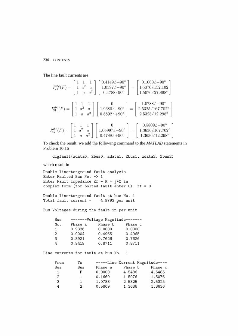
236 CONTENTS
The line fault currents are
Iabc21 (F ) =
1 1 11 a2 a1 a a2
0.41496 +901.05976 −900.47886 90
=
0.16606 −901.50766 152.1021.5076 6 27.898
Iabc31 (F ) =
1 1 11 a2 a1 a a2
01.96806 −900.88926 +90
=
1.07886 −902.53256 167.7022.5325 6 12.298
Iabc42 (F ) =
1 1 11 a2 a1 a a2
01.059976 −900.47886 +90
=
0.5809 6 −901.3636 6 167.7021.36366 12.298
To check the result, we add the following command to theMATLABstatements inProblem 10.16
dlgfault(zdata0, Zbus0, zdata1, Zbus1, zdata2, Zbus2)
which result in
Double line-to-ground fault analysisEnter Faulted Bus No. -> 1Enter Fault Impedance Zf = R + j*X incomplex form (for bolted fault enter 0). Zf = 0
Double line-to-ground fault at bus No. 1Total fault current = 4.9793 per unit
Bus Voltages during the fault in per unit
Bus -------Voltage Magnitude-------No. Phase a Phase b Phase c1 0.9336 0.0000 0.00002 0.9004 0.4965 0.49653 0.8921 0.7626 0.76264 0.9419 0.8711 0.8711
Line currents for fault at bus No. 1
From To -----Line Current Magnitude----Bus Bus Phase a Phase b Phase c1 F 0.0000 4.5486 4.54852 1 0.1660 1.5076 1.50763 1 1.0788 2.5325 2.53254 2 0.5809 1.3636 1.3636
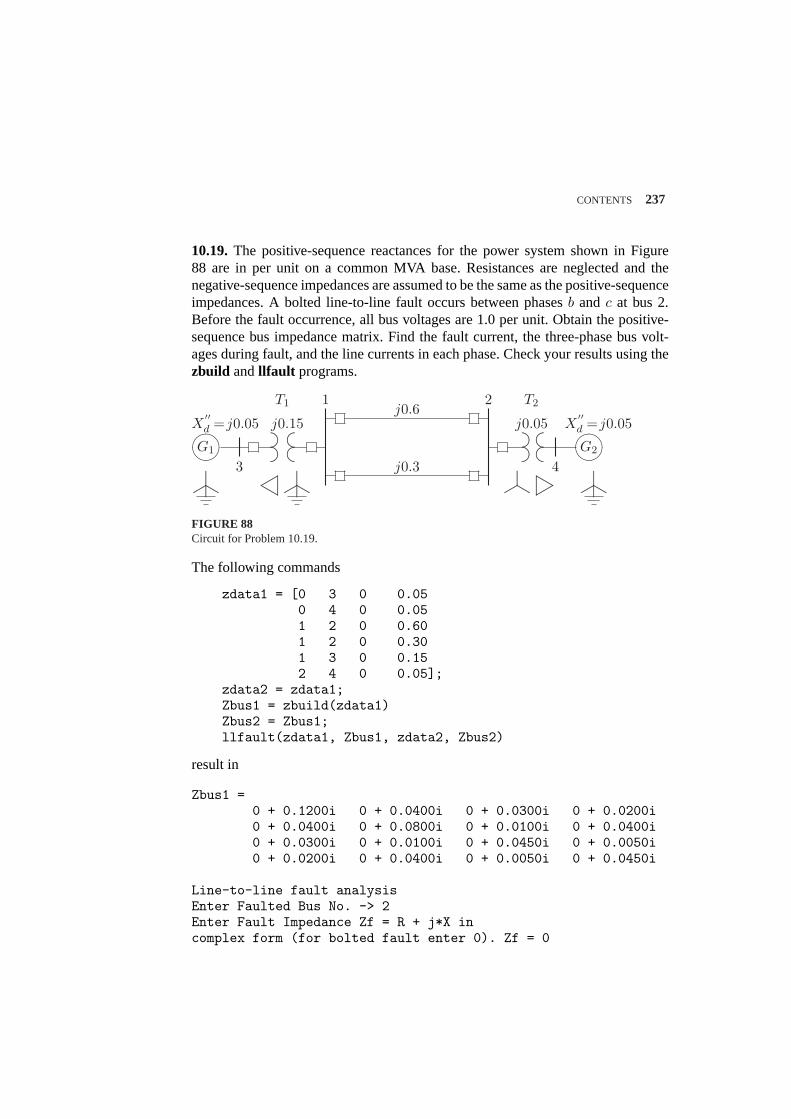
CONTENTS 237
10.19.The positive-sequence reactances for the power system shown in Figure88 are in per unit on a common MVA base. Resistances are neglected and thenegative-sequence impedances are assumed to be the same as the positive-sequenceimpedances. A bolted line-to-line fault occurs between phasesb and c at bus 2.Before the fault occurrence, all bus voltages are 1.0 per unit. Obtain the positive-sequence bus impedance matrix. Find the fault current, the three-phase bus volt-ages during fault, and the line currents in each phase. Check your results using thezbuild andllfault programs.
µ´¶³
...................................................................................... ...................................................................................... ................
........
.............................................................. ...................................................................................... µ´
¶³
.................................................................
........................................................
..........................................................................
.....................
.................................................................
........................................
............................................
........................................
..................................................................................
........
........
........
......................................................
........................................................
G1 G2
T1 T2
3
1 2
4
X′′d =j0.05 j0.15
j0.6
j0.3
j0.05 X′′d =j0.05
FIGURE 88Circuit for Problem 10.19.
The following commands
zdata1 = [0 3 0 0.050 4 0 0.051 2 0 0.601 2 0 0.301 3 0 0.152 4 0 0.05];
zdata2 = zdata1;Zbus1 = zbuild(zdata1)Zbus2 = Zbus1;llfault(zdata1, Zbus1, zdata2, Zbus2)
result in
Zbus1 =0 + 0.1200i 0 + 0.0400i 0 + 0.0300i 0 + 0.0200i0 + 0.0400i 0 + 0.0800i 0 + 0.0100i 0 + 0.0400i0 + 0.0300i 0 + 0.0100i 0 + 0.0450i 0 + 0.0050i0 + 0.0200i 0 + 0.0400i 0 + 0.0050i 0 + 0.0450i
Line-to-line fault analysisEnter Faulted Bus No. -> 2Enter Fault Impedance Zf = R + j*X incomplex form (for bolted fault enter 0). Zf = 0
238 CONTENTS
Line-to-line fault at bus No. 2Total fault current = 10.8253 per unit
Bus Voltages during the fault in per unit
Bus -------Voltage Magnitude-------No. Phase a Phase b Phase c1 1.0000 0.6614 0.66142 1.0000 0.5000 0.50003 1.0000 0.9079 0.90794 1.0000 0.6614 0.6614
Line currents for fault at bus No. 2
From To -----Line Current Magnitude----Bus Bus Phase a Phase b Phase c1 2 0.0000 0.7217 0.72171 2 0.0000 1.4434 1.44342 F 0.0000 10.8253 10.82533 1 0.0000 2.1651 2.16514 2 0.0000 8.6603 8.6603
Another fault location? Enter’y’ or’n’ within single quote->’n’
10.20.Use thelgfault , llfault , anddlgfault functions to compute the fault current,bus voltages, and line currents in the circuit given in Example 10.8 for the followingunbalanced fault.(a) A bolted single line-to-ground fault at bus 9.(b) A bolted line-to-line fault at bus 9.(c) A bolted double line-to-ground fault at bus 9.All shunt capacitances and loads are neglected and the negative-sequence data isassumed to be the same as the positive-sequence data. All the prefault bus voltagesare assumed to be unity.
Run chp10ex8 for a bolted fault at bus 9ch10p20.
10.21.The six-bus power system network of an electric utility company is shown inFigure 89. The positive- and zero-sequence reactances of the lines and transform-ers in per unit on a 100-MVA base is tabulated below. The transformer connectionsare shown in Figure 89. The∆-Y transformer between buses 3 and 5 is groundedthrough a reactor of reactance 0.10 per unit. The generator’s positive- and zero-sequence reactances including the reactance of grounding neutrals on a 100-MVAbase is tabulated below.
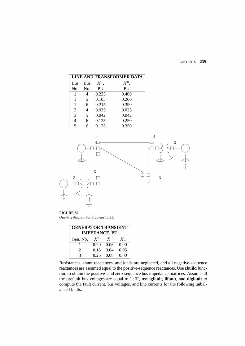
CONTENTS 239
LINE AND TRANSFORMER DATABus Bus X1, X0,No. No. PU PU1 4 0.225 0.4001 5 0.105 0.2001 6 0.215 0.3902 4 0.035 0.0353 5 0.042 0.0424 6 0.125 0.2505 6 0.175 0.350
µ´¶³
...................................................................................... ...................................................................................... µ´
¶³........................................................................................................................................................................................................................................................................................................................
µ´¶³
...................................................................................... ......................................................................................
........................................................ ................
........................................
................................................................
........
........
....
........................................................
.............................................
........................................................
................................................................
........
........
....
........................................................
.............................................
12
3
4
56
FIGURE 89One-line diagram for Problem 10.21.
GENERATOR TRANSIENTIMPEDANCE, PU
Gen. No. X1 X0 Xn
1 0.20 0.06 0.002 0.15 0.04 0.053 0.25 0.08 0.00
Resistances, shunt reactances, and loads are neglected, and all negative-sequencereactances are assumed equal to the positive-sequence reactances. Usezbuild func-tion to obtain the positive- and zero-sequence bus impedance matrices. Assume allthe prefault bus voltages are equal to16 0, uselgfault , llfault , anddlgfault tocompute the fault current, bus voltages, and line currents for the following unbal-anced faults.
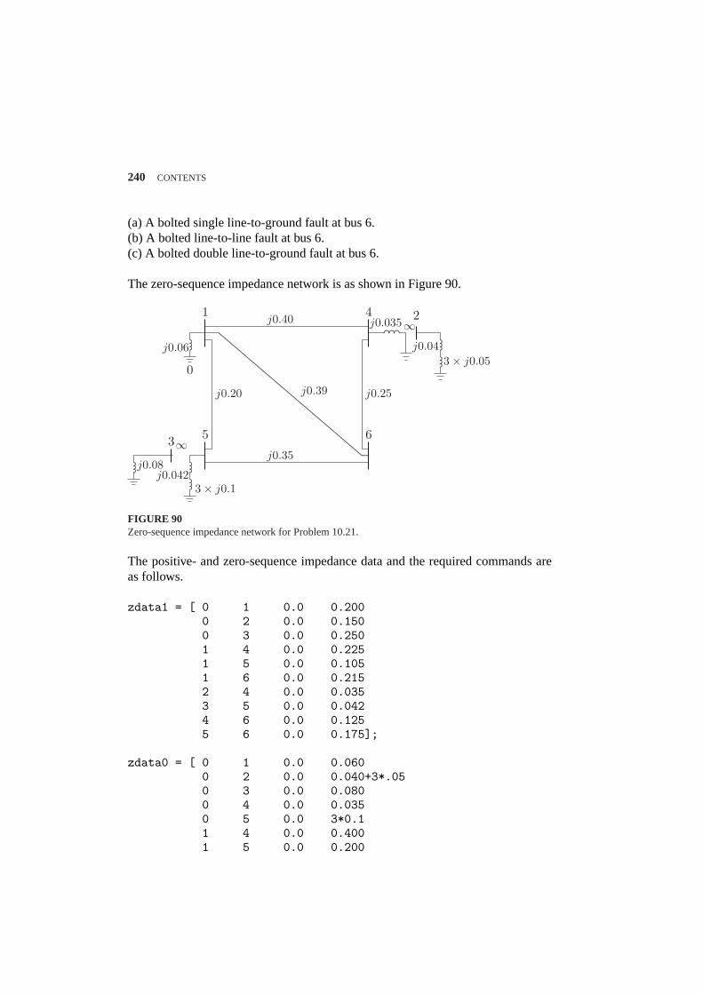
240 CONTENTS
(a) A bolted single line-to-ground fault at bus 6.(b) A bolted line-to-line fault at bus 6.(c) A bolted double line-to-ground fault at bus 6.
The zero-sequence impedance network is as shown in Figure 90.
0
...............................................................................................................................................................................................................................................................................................................................................................................................................................
....................................
....................................
........................................................................
......................................................
........................................................................
1 4 2
5 63
j0.06
j0.08j0.042
3× j0.1
j0.043× j0.05
j0.40
j0.35
j0.39j0.20 j0.25
j0.035∞
∞
FIGURE 90Zero-sequence impedance network for Problem 10.21.
The positive- and zero-sequence impedance data and the required commands areas follows.
zdata1 = [ 0 1 0.0 0.2000 2 0.0 0.1500 3 0.0 0.2501 4 0.0 0.2251 5 0.0 0.1051 6 0.0 0.2152 4 0.0 0.0353 5 0.0 0.0424 6 0.0 0.1255 6 0.0 0.175];
zdata0 = [ 0 1 0.0 0.0600 2 0.0 0.040+3*.050 3 0.0 0.0800 4 0.0 0.0350 5 0.0 3*0.11 4 0.0 0.4001 5 0.0 0.200
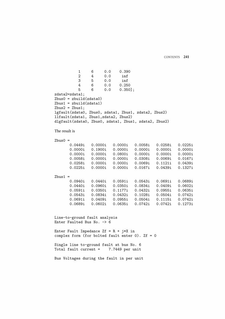
CONTENTS 241
1 6 0.0 0.3902 4 0.0 inf3 5 0.0 inf4 6 0.0 0.2505 6 0.0 0.350];
zdata2=zdata1;Zbus0 = zbuild(zdata0)Zbus1 = zbuild(zdata1)Zbus2 = Zbus1;lgfault(zdata0, Zbus0, zdata1, Zbus1, zdata2, Zbus2)llfault(zdata1, Zbus1,zdata2, Zbus2)dlgfault(zdata0, Zbus0, zdata1, Zbus1, zdata2, Zbus2)
The result is
Zbus0 =0.0449i 0.0000i 0.0000i 0.0058i 0.0258i 0.0225i0.0000i 0.1900i 0.0000i 0.0000i 0.0000i 0.0000i0.0000i 0.0000i 0.0800i 0.0000i 0.0000i 0.0000i0.0058i 0.0000i 0.0000i 0.0308i 0.0069i 0.0167i0.0258i 0.0000i 0.0000i 0.0069i 0.1121i 0.0439i0.0225i 0.0000i 0.0000i 0.0167i 0.0439i 0.1327i
Zbus1 =0.0940i 0.0440i 0.0591i 0.0543i 0.0691i 0.0689i0.0440i 0.0960i 0.0350i 0.0834i 0.0409i 0.0602i0.0591i 0.0350i 0.1177i 0.0432i 0.0955i 0.0635i0.0543i 0.0834i 0.0432i 0.1028i 0.0504i 0.0742i0.0691i 0.0409i 0.0955i 0.0504i 0.1115i 0.0742i0.0689i 0.0602i 0.0635i 0.0742i 0.0742i 0.1273i
Line-to-ground fault analysisEnter Faulted Bus No. -> 6
Enter Fault Impedance Zf = R + j*X incomplex form (for bolted fault enter 0). Zf = 0
Single line to-ground fault at bus No. 6Total fault current = 7.7449 per unit
Bus Voltages during the fault in per unit
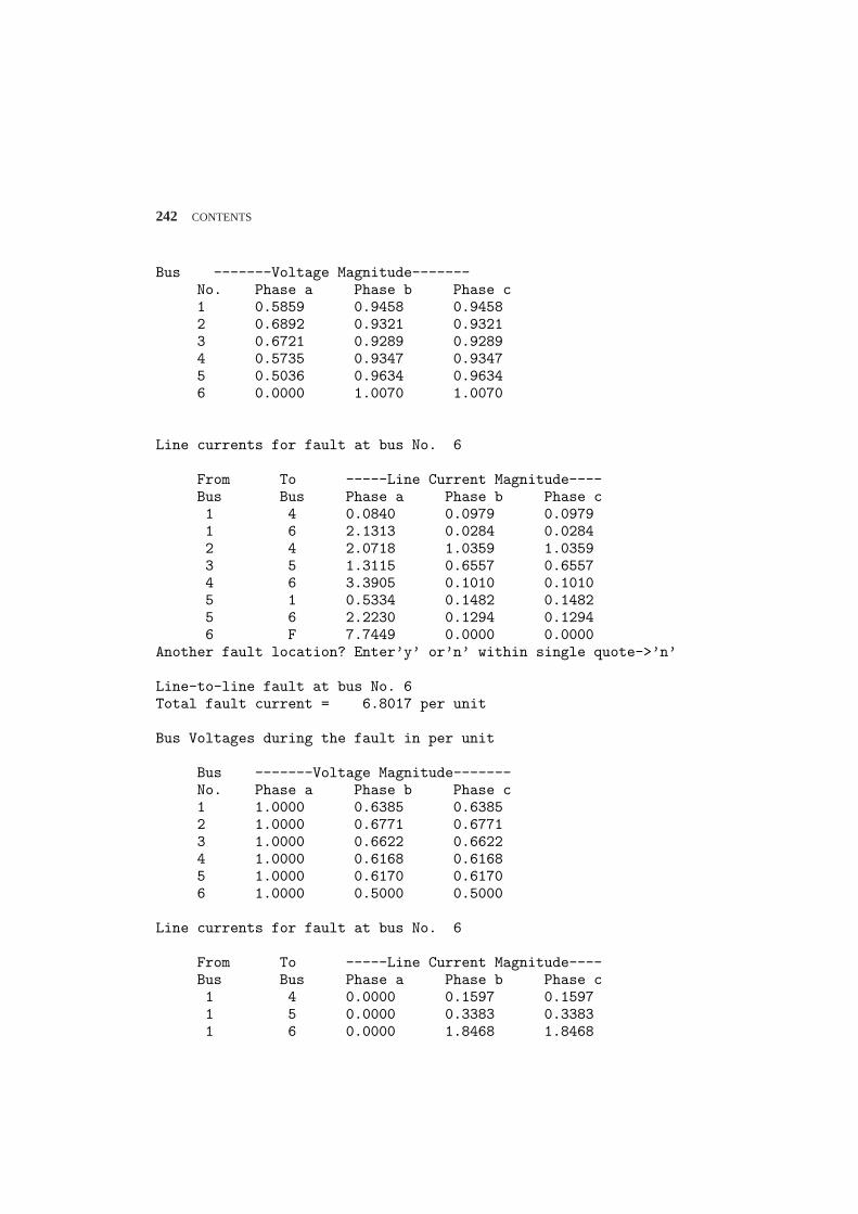
242 CONTENTS
Bus -------Voltage Magnitude-------No. Phase a Phase b Phase c1 0.5859 0.9458 0.94582 0.6892 0.9321 0.93213 0.6721 0.9289 0.92894 0.5735 0.9347 0.93475 0.5036 0.9634 0.96346 0.0000 1.0070 1.0070
Line currents for fault at bus No. 6
From To -----Line Current Magnitude----Bus Bus Phase a Phase b Phase c1 4 0.0840 0.0979 0.09791 6 2.1313 0.0284 0.02842 4 2.0718 1.0359 1.03593 5 1.3115 0.6557 0.65574 6 3.3905 0.1010 0.10105 1 0.5334 0.1482 0.14825 6 2.2230 0.1294 0.12946 F 7.7449 0.0000 0.0000
Another fault location? Enter’y’ or’n’ within single quote->’n’
Line-to-line fault at bus No. 6Total fault current = 6.8017 per unit
Bus Voltages during the fault in per unit
Bus -------Voltage Magnitude-------No. Phase a Phase b Phase c1 1.0000 0.6385 0.63852 1.0000 0.6771 0.67713 1.0000 0.6622 0.66224 1.0000 0.6168 0.61685 1.0000 0.6170 0.61706 1.0000 0.5000 0.5000
Line currents for fault at bus No. 6
From To -----Line Current Magnitude----Bus Bus Phase a Phase b Phase c1 4 0.0000 0.1597 0.15971 5 0.0000 0.3383 0.33831 6 0.0000 1.8468 1.8468
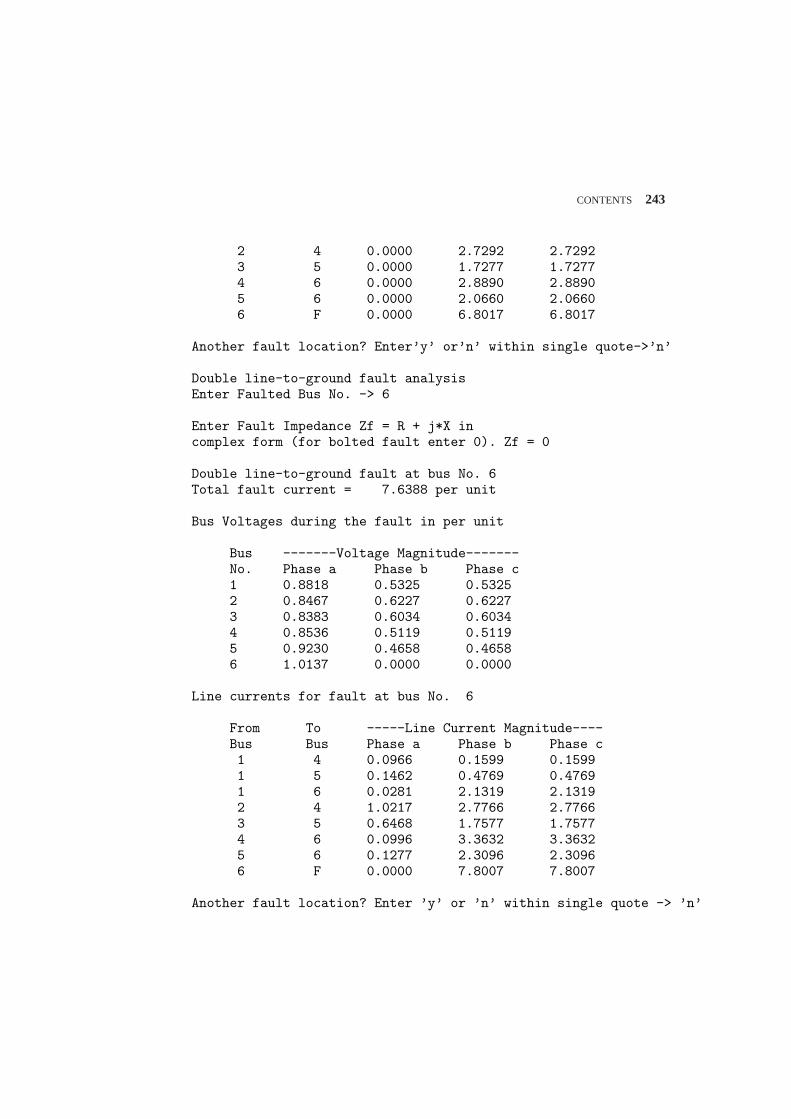
CONTENTS 243
2 4 0.0000 2.7292 2.72923 5 0.0000 1.7277 1.72774 6 0.0000 2.8890 2.88905 6 0.0000 2.0660 2.06606 F 0.0000 6.8017 6.8017
Another fault location? Enter’y’ or’n’ within single quote->’n’
Double line-to-ground fault analysisEnter Faulted Bus No. -> 6
Enter Fault Impedance Zf = R + j*X incomplex form (for bolted fault enter 0). Zf = 0
Double line-to-ground fault at bus No. 6Total fault current = 7.6388 per unit
Bus Voltages during the fault in per unit
Bus -------Voltage Magnitude-------No. Phase a Phase b Phase c1 0.8818 0.5325 0.53252 0.8467 0.6227 0.62273 0.8383 0.6034 0.60344 0.8536 0.5119 0.51195 0.9230 0.4658 0.46586 1.0137 0.0000 0.0000
Line currents for fault at bus No. 6
From To -----Line Current Magnitude----Bus Bus Phase a Phase b Phase c1 4 0.0966 0.1599 0.15991 5 0.1462 0.4769 0.47691 6 0.0281 2.1319 2.13192 4 1.0217 2.7766 2.77663 5 0.6468 1.7577 1.75774 6 0.0996 3.3632 3.36325 6 0.1277 2.3096 2.30966 F 0.0000 7.8007 7.8007
Another fault location? Enter ’y’ or ’n’ within single quote -> ’n’
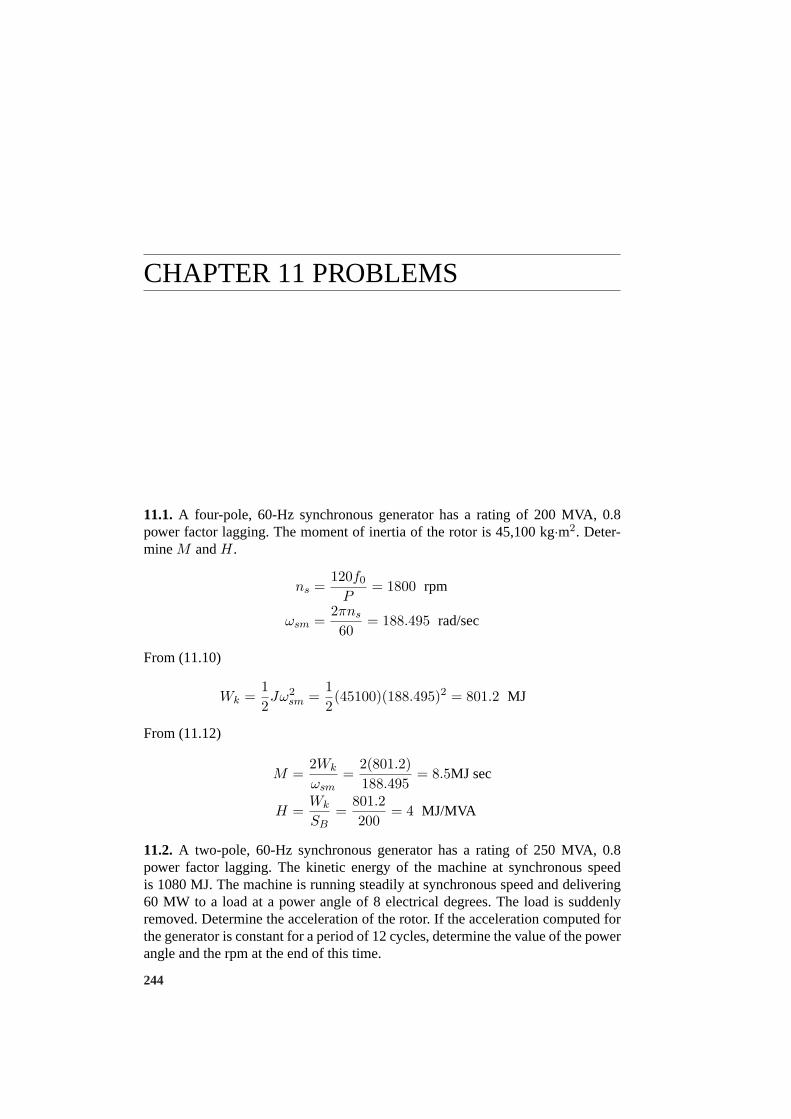
CHAPTER 11 PROBLEMS
11.1. A four-pole, 60-Hz synchronous generator has a rating of 200 MVA, 0.8power factor lagging. The moment of inertia of the rotor is 45,100 kg·m2. Deter-mineM andH.
ns =120f0
P= 1800 rpm
ωsm =2πns
60= 188.495 rad/sec
From (11.10)
Wk =12Jω2
sm =12(45100)(188.495)2 = 801.2 MJ
From (11.12)
M =2Wk
ωsm=
2(801.2)188.495
= 8.5MJ sec
H =Wk
SB=
801.2200
= 4 MJ/MVA
11.2. A two-pole, 60-Hz synchronous generator has a rating of 250 MVA, 0.8power factor lagging. The kinetic energy of the machine at synchronous speedis 1080 MJ. The machine is running steadily at synchronous speed and delivering60 MW to a load at a power angle of 8 electrical degrees. The load is suddenlyremoved. Determine the acceleration of the rotor. If the acceleration computed forthe generator is constant for a period of 12 cycles, determine the value of the powerangle and the rpm at the end of this time.
244
CONTENTS 245
H =Wk
SB=
1080250
= 4.32 MJ/MVA
Pm =60250
= 0.24 pu
12 cycle=1260
= 0.2 sec
From (11.22)
H
180f
d2δ
dt2= 0.24− 0
or
d2δ
dt2= 600 degree/sec2
=60360
(600) = 100 rpm/sec
Integrating the above expression, we have
dδ
dt= 600t
δ =12(600)t2 + δ0
=12(600)(0.2)2 + 8 = 20
ns =120f0
P=
(120)(60)2
= 3600 rpm
Speed at the end of 0.2 second is
n = 3600 + 0.2(100) = 3620 rpm
11.3.Determine the kinetic energy stored by a 250-MVA, 60-Hz, two-pole syn-chronous generator with an inertia constantH of 5.4 MJ/MVA. Assume the ma-chine is running steadily at synchronous speed with a shaft input of 331,100 hpThe electrical power developed suddenly changes from its normal value to a value
246 CONTENTS
of 200 MW. Determine the acceleration or deceleration of the rotor. If the acceler-ation computed for the generator is constant for a period of 9 cycles, determine thechange in the power angle in that period and the rpm at the end of 9 cycles.
Pm = (331100)(746)(10−6) = 247 MW
=247250
= 0.988 pu
Pe =200250
= 0.8 pu
9 cycle=960
= 0.15 sec
From (11.22), we have
5.4(180(60)
d2δ
dt2= 0.988− 0.8
or
d2δ
dt2= 376 degree/sec2
=60360
(736) = 62.6667 rpm/sec
Integrating the above expression, we have
dδ
dt= 376t
δ =12(376)t2 + δ0
=12(376)(0.15)2 + δ0
or
∆δ = δ − δ0 == 4.23
ns =120f0
P=
(120)(60)2
= 3600 rpm
Speed at the end of 0.15 second is
n = 3600 + 0.15(62.6667) = 3609.4 rpm
CONTENTS 247
11.4.The swing equations of two interconnected synchronous machines are writtenas
H1
πf0
d2δ1
dt2= Pm1 − Pe1
H2
πf0
d2δ2
dt2= Pm2 − Pe2
Denote the relative power angle between the two machines byδ = δ1− δ2. Obtaina swing equation equivalent to that of a single machine in terms ofδ, and show that
H
πf0
d2δ
dt2= Pm − Pe
where
H =H1H2
H1 + H2
Pm =H2Pm1 −H1Pm2
H1 + H2and Pe =
H2Pe1 −H1Pe2
H1 + H2
Subtracting the second swing equation from the first, we obtain
1πf0
(d2δ1
dt2− d2δ2
dt2
)=
(Pm1
H1− Pm2
H2
)−
(Pe1
H1− Pe2
H2
)
or
1πf0
(d2(δ1 − δ2)
dt2
)=
(H2Pm1 −H1Pm2
H1H2
)−
(H2Pe1 −H1Pe2
H1H2
)
Multiplying both side by H1H2H1+H2
, results in
1πf0
H1H2
H1 + H2
(d2(δ1 − δ2)
dt2
)=
(H2Pm1 −H1Pm2
H1 + H2
)−
(H2Pe1 −H1Pe2
H1 + H2
)
or
H
πf0
d2δ
dt2= Pm − Pe
whereH, δ, Pm, andPe are defined above.
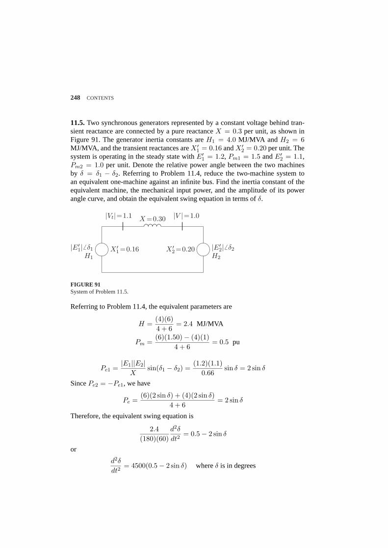
248 CONTENTS
11.5.Two synchronous generators represented by a constant voltage behind tran-sient reactance are connected by a pure reactanceX = 0.3 per unit, as shown inFigure 91. The generator inertia constants areH1 = 4.0 MJ/MVA and H2 = 6MJ/MVA, and the transient reactances areX ′
1 = 0.16 andX ′2 = 0.20 per unit. The
system is operating in the steady state withE′1 = 1.2, Pm1 = 1.5 andE′
2 = 1.1,Pm2 = 1.0 per unit. Denote the relative power angle between the two machinesby δ = δ1 − δ2. Referring to Problem 11.4, reduce the two-machine system toan equivalent one-machine against an infinite bus. Find the inertia constant of theequivalent machine, the mechanical input power, and the amplitude of its powerangle curve, and obtain the equivalent swing equation in terms ofδ.
µ´¶³
|E′1|6 δ1
H1
X ′1 =0.16 µ´
¶³|E′
2|6 δ2
H2
X ′2 =0.20
....................................
....................................................
................
X =0.30|Vt|=1.1 |V |=1.0
FIGURE 91System of Problem 11.5.
Referring to Problem 11.4, the equivalent parameters are
H =(4)(6)4 + 6
= 2.4 MJ/MVA
Pm =(6)(1.50)− (4)(1)
4 + 6= 0.5 pu
Pe1 =|E1||E2|
Xsin(δ1 − δ2) =
(1.2)(1.1)0.66
sin δ = 2 sin δ
SincePe2 = −Pe1, we have
Pe =(6)(2 sin δ) + (4)(2 sin δ)
4 + 6= 2 sin δ
Therefore, the equivalent swing equation is
2.4(180)(60)
d2δ
dt2= 0.5− 2 sin δ
or
d2δ
dt2= 4500(0.5− 2 sin δ) whereδ is in degrees
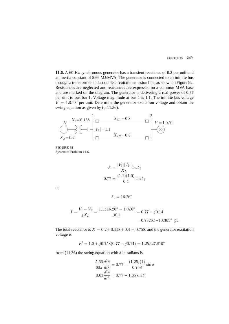
CONTENTS 249
11.6.A 60-Hz synchronous generator has a transient reactance of 0.2 per unit andan inertia constant of 5.66 MJ/MVA. The generator is connected to an infinite busthrough a transformer and a double circuit transmission line, as shown in Figure 92.Resistances are neglected and reactances are expressed on a common MVA baseand are marked on the diagram. The generator is delivering a real power of 0.77per unit to bus bar 1. Voltage magnitude at bus 1 is 1.1. The infinite bus voltageV = 1.06 0 per unit. Determine the generator excitation voltage and obtain theswing equation as given by (pr11.36).
µ´¶³
...................................................................................... ...................................................................................... µ´
¶³
X ′d =0.2
Xt =0.158 XL1 =0.8
XL2 =0.8∞
E′ V =1.0 6 0
|V1|=1.1
1 2
FIGURE 92System of Problem 11.6.
P =|V1||V2|
XLsin δ1
0.77 =(1.1)(1.0)
0.4sin δ1
or
δ1 = 16.26
I =V1 − V2
jXL=
1.16 16.26 − 1.0 6 0
j0.4= 0.77− j0.14
= 0.78266 −10.305 pu
The total reactance isX = 0.2+0.158+0.4 = 0.758, and the generator excitationvoltage is
E′ = 1.0 + j0.758(0.77− j0.14) = 1.25 6 27.819
from (11.36) the swing equation withδ in radians is
5.6660π
d2δ
dt2= 0.77− (1.25)(1)
0.758sin δ
0.03d2δ
dt2= 0.77− 1.65 sin δ
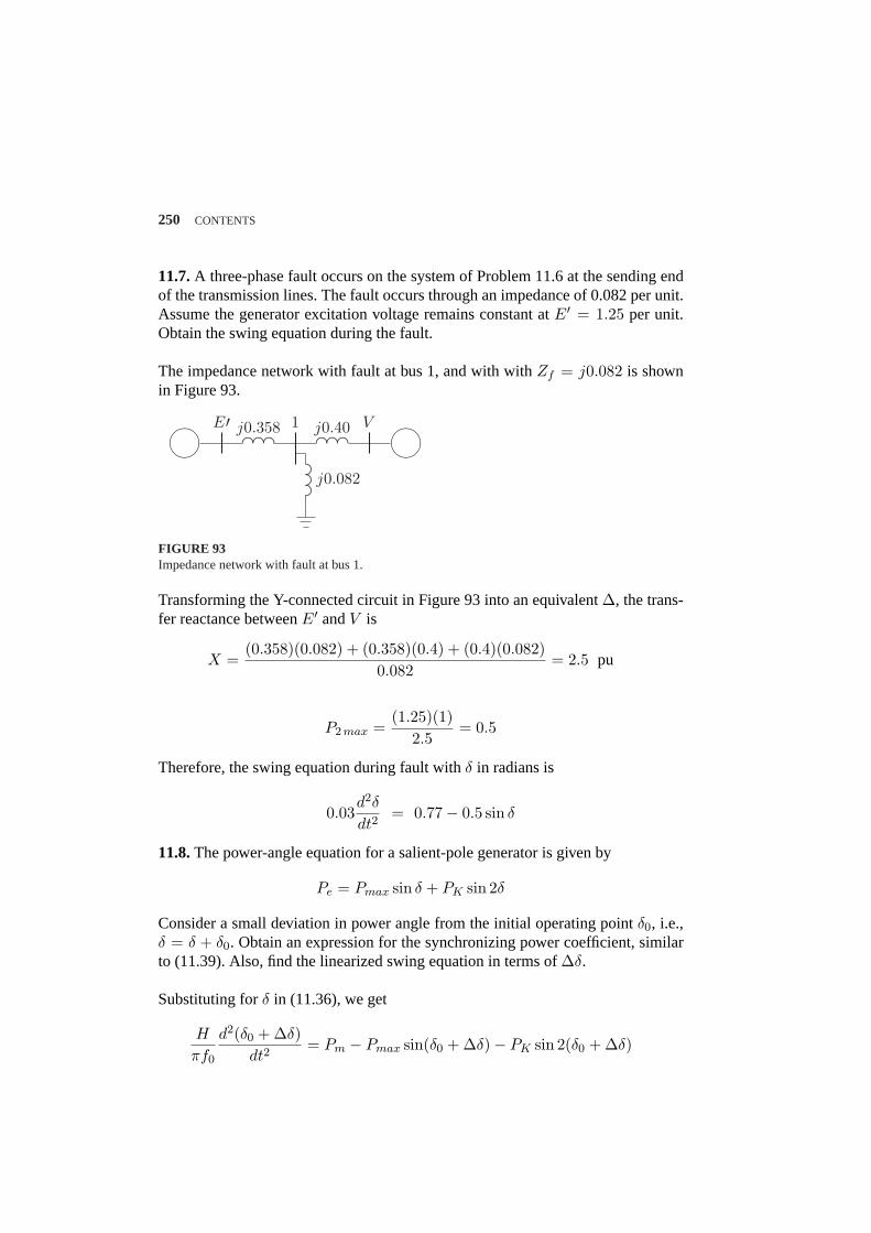
250 CONTENTS
11.7.A three-phase fault occurs on the system of Problem 11.6 at the sending endof the transmission lines. The fault occurs through an impedance of 0.082 per unit.Assume the generator excitation voltage remains constant atE′ = 1.25 per unit.Obtain the swing equation during the fault.
The impedance network with fault at bus 1, and with withZf = j0.082 is shownin Figure 93.
µ´¶³
.......................................
................................................ ..........
..........................................................
...................
µ´¶³
.......................................................................................
1E′ Vj0.358 j0.40
j0.082
FIGURE 93Impedance network with fault at bus 1.
Transforming the Y-connected circuit in Figure 93 into an equivalent∆, the trans-fer reactance betweenE′ andV is
X =(0.358)(0.082) + (0.358)(0.4) + (0.4)(0.082)
0.082= 2.5 pu
P2 max =(1.25)(1)
2.5= 0.5
Therefore, the swing equation during fault withδ in radians is
0.03d2δ
dt2= 0.77− 0.5 sin δ
11.8.The power-angle equation for a salient-pole generator is given by
Pe = Pmax sin δ + PK sin 2δ
Consider a small deviation in power angle from the initial operating pointδ0, i.e.,δ = δ + δ0. Obtain an expression for the synchronizing power coefficient, similarto (11.39). Also, find the linearized swing equation in terms of∆δ.
Substituting forδ in (11.36), we get
H
πf0
d2(δ0 + ∆δ)dt2
= Pm − Pmax sin(δ0 + ∆δ)− PK sin 2(δ0 + ∆δ)
CONTENTS 251
or
H
πf0
d2δ0
dt2+
H
πf0
d2∆δ
dt2= Pm − Pmax(sin δ0 cos∆δ + cos δ0 sin∆δ)−
PK(sin 2δ0 cos 2∆δ + cos 2δ0 sin 2∆δ)
Since∆δ is small,cos 2∆δ ∼= 1, cos∆δ ∼= 1, sin 2∆δ ∼= 2∆δ andsin∆δ ∼= ∆δ,and we have
H
πf0
d2δ0
dt2+
H
πf0
d2∆δ
dt2= Pm − Pmax sin δ0 − Pmax cos δ0 (∆δ)−
PK sin 2δ0 − PK cos 2δ0 (2∆δ)
Since at the initial operating state
H
πf0
d2δ0
dt2= Pm − Pmax sin δ0 − PK sin 2δ0
The above equation reduces to linearized equation in terms of incremental changesin power angle, i.e.,
H
πf0
d2∆δ
dt2+ (Pmax cos δ0 + 2PK cos 2δ0)∆δ = 0
or
H
πf0
d2∆δ
dt2+ PS∆δ = 0
wherePS is the slope of the power-angle curve atδ0, known as thesynchronizingpower coefficient, given by
Ps =dP
dδ
∣∣∣∣δ0
= Pmax cos δ0 + 2PK cos 2δ0
11.9.Consider the displacementx for a unit mass supported by a nonlinear springas shown in Figure 94. The equation of motion is described by
Md2x(t)
dt2+ B
dx(t)dt
+ K sinx(t) = f(t)
whereM is the mass,B is the frictional coefficient andK is the spring constant.The system is at the steady statex(0) = 0 for f(0) = 0. A small perturbationf(t) = f(0) + ∆f(t) results in the displacementx(t) = x(0) + ∆x(t).(a) Obtain a linearized expression for the motion of the system in terms of the sys-tem parameters,∆x(t) and∆f(t).
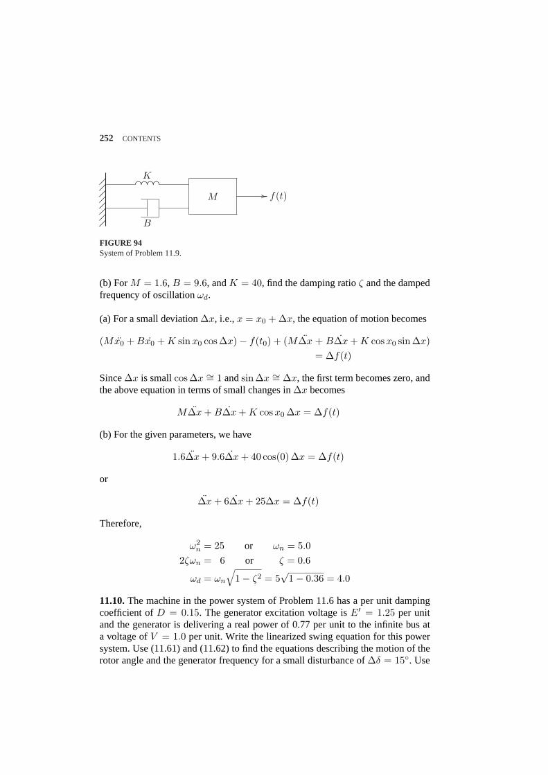
252 CONTENTS
....................................
....................................................
................
.................................................................................................. ................
.......................
.......................
.......................
.......................
.......................
.......................
.......................
.......................
K
B
M f(t)
FIGURE 94System of Problem 11.9.
(b) ForM = 1.6, B = 9.6, andK = 40, find the damping ratioζ and the dampedfrequency of oscillationωd.
(a) For a small deviation∆x, i.e.,x = x0 + ∆x, the equation of motion becomes
(Mx0 + Bx0 + K sinx0 cos∆x)− f(t0) + (M∆x + B∆x + K cosx0 sin∆x)= ∆f(t)
Since∆x is smallcos∆x ∼= 1 andsin∆x ∼= ∆x, the first term becomes zero, andthe above equation in terms of small changes in∆x becomes
M∆x + B∆x + K cosx0 ∆x = ∆f(t)
(b) For the given parameters, we have
1.6∆x + 9.6∆x + 40 cos(0)∆x = ∆f(t)
or
∆x + 6∆x + 25∆x = ∆f(t)
Therefore,
ω2n = 25 or ωn = 5.0
2ζωn = 6 or ζ = 0.6
ωd = ωn
√1− ζ2 = 5
√1− 0.36 = 4.0
11.10.The machine in the power system of Problem 11.6 has a per unit dampingcoefficient ofD = 0.15. The generator excitation voltage isE′ = 1.25 per unitand the generator is delivering a real power of 0.77 per unit to the infinite bus ata voltage ofV = 1.0 per unit. Write the linearized swing equation for this powersystem. Use (11.61) and (11.62) to find the equations describing the motion of therotor angle and the generator frequency for a small disturbance of∆δ = 15. Use
CONTENTS 253
MATLABto obtain the plots of rotor angle and frequency.
The initial operating angle is given by
0.77 =(1.25)(1)
0.758sin δ or δ = 27.835 = 0.4858 radian
The synchronizing power coefficient given by (11.39) is
Ps = Pmax cos δ0 =(1.25)(1)
0.758cos 27.835 = 1.4583
The undamped angular frequency of oscillation and damping ratio are
ωn =
√πf0
HPs =
√(π)(60)
5.661.4583 = 6.969 rad/sec
ζ =D
2
√πf0
HPs=
0.152
√(π)(60)
(5.66)(1.4583)= 0.3584
The linearized force-free equation which determines the mode of oscillation givenby (11.46) withδ in radian is
d2∆δ
dt2+ 5
d∆δ
dt+ 48.565∆δ = 0
From (11.50), the damped angular frequency of oscillation is
ωd = ωn
√1− ζ2 = 6.969
√1− (0.3584)2 = 6.506 rad/sec
corresponding to a damped oscillation frequency of
fd =6.5062π
= 1.035 Hz
θ = cos−1 0.3584 = 69
From (11.61) and (11.62), the motion of rotor relative to the synchronously re-volving field in electrical degrees and the frequency excursion in Hz are given byequations
δ = 27.835 + 16.0675e−2.4977t sin (6.506t + 69)f = 60− 0.311e−2.4977t sin 6.506t
Use the following commands to obtain the plots of rotor angle and frequency
254 CONTENTS
t = 0:.01:3;d=27.835+16.0675*exp(-2.4977*t).*sin(6.506*t+69*pi/180);f = 60 - 0.311*exp(-2.4977*t).*sin(6.506*t);figure(1), plot(t, d), gridxlabel(’t, sec.’), ylabel(’Delta, degree’)figure(2) , plot(t,f), gridxlabel(’t, sec.’), ylabel(’f, Hz’)
11.11.Write the linearized swing equation of Problem 11.10 in state variable form.Use[y, x] = initial( A,B,C, D, x0, t) andplot commands to obtain the zero-inputresponse for the initial conditions∆δ = 15, and∆ωn = 0.
From (11-52)–(11.55), we have
A =[
0 1−48.5649 −4.9955
]B =
[00
]C =
[1 00 1
]D =
[00
]
Use the following commands to obtain the plots of rotor angle and frequency
A = [0 1; -48.5649 -4.9955];B = [0; 0]; C = [1 0; 0 1]; D = [0; 0];Dd0 = 15*pi/180; % Initial angle in radianDx0 = [Dd0; 0]; % Initial conditionst = 0:.01:3;[y,x]= initial(A, B, C, D, Dx0, t);Dd = x(:, 1); Dw = x(:, 2); % State variables x1 and x2d = 27.835 + Dd*180/pi; % power angle in degreef = 60 + Dw/(2*pi); % Frequency in Hzfigure(1), plot(t, d), gridxlabel(’t, sec’), ylabel(’Delta, degree’)figure(2), plot(t, f), gridxlabel(’t, sec’), ylabel(’f, Hz’)
11.12.The generator of Problem 11.10 is operating in the steady state atδ0 =27.835 when the input power is increased by a small amount∆P = 0.15 per unit.The generator excitation and the infinite bus voltage are the same as before. Use(11.75) and (11.76) to find the equations describing the motion of the rotor angleand the generator frequency for a small disturbance of∆P = 0.15 per unit. UseMATLABto obtain the plots of rotor angle and frequency.
(a) Substituting forH, δ0, ζ, andωn evaluated in Problem 11.11 in (11.75), andexpressing the power angle in degree, we get
δ = 27.835 +(180)(60)(0.15)(5.66)(48.565)
[1− 1√1− (0.3548)2
e−2.4977t sin(6.506t + 69)]
CONTENTS 255
or
δ = 27.835 + 5.8935[1− 1.0712e−2.4977t sin(6.506t + 69)]
Also, substituting the values in (11.76) and expressing the frequency in Hz, we get
f = 60 +(60)(0.15)
2(5.66)(6.506)√
1− (0.3584)2e−2.4977t sin 6.506t
or
f = 60 + 0.1222e−2.4977t sin 6.506t
Plot δ, andf over a range of0 to 3 seconds.
11.13.Write the linearized swing equation of Problem 11.10 in state variable form.Use[y, x] = step(A,B, C,D, 1, t) andplot commands to obtain the zero-state re-sponse when the input power is increased by a small amount∆P = 0.15 per unit.
From (11.70), the state equation for Problem 11.13 is
[x1
x2
]=
[0 1
−48.5649 −4.9955
] [x1
x2
]+
[01
]∆u
and
y =[
1 00 1
] [x1
x2
]
From (11.69),∆u = (60π/5.66)(0.15) = 4.9955. The followingMATLABcom-mands are used to obtain the step response for Example 11.13.
Du = pi*60/5.66*0.15; % Small step change in power inputA = [0 1; -48.5649 -4.9955];B = [0;1]*Du; C = [1 0; 0 1];D = [0; 0];t = 0:.01:3;[y, x] = step(A, B, C, D, 1, t);Dd = x(:, 1); Dw = x(:, 2); % State variables x1 and x2d = 27.835 + Dd*180/pi; % Power angle in degreef = 60 + Dw/(2*pi); % Frequency in Hzfigure(1), plot(t, d), gridxlabel(’t, sec’), ylabel(’Delta, degree’)figure(2), plot(t, f), gridxlabel(’t, sec’), ylabel(’f, Hz’)
256 CONTENTS
11.14.The machine of Problem 11.6 is delivering a real power input of 0.77 perunit to the infinite bus at a voltage of 1.0 per unit. The generator excitation voltageis E′ = 1.25 per unit. Useeacpower(Pm, E, V,X) to find(a) The maximum power input that can be added without loss of synchronism.(b) Repeat (a) with zero initial power input. Assume the generator internal voltageremains constant at the value computed in (a).
In Problem 11.6, the transfer reactance and the generator internal voltage werefound to beX = 0.758 pu, andE′ = 1.25 pu.
We use the following commands
disp(’(a) Initial real power P0 = 0.77’)P0 = 0.77; E = 1.25; V = 1.0; X = 0.758;h=figure;eacpower(P0, E, V, X)h=figure;disp(’(b) Zero initial power ’)P0 = 0;eacpower(P0, E, V, X)
which result in
(a) Initial real power P0 = 0.77Initial power = 0.770 p.u.Initial power angle = 27.835 degreesSudden additional power = 0.649 p.u.Total power for critical stability = 1.419 p.u.Maximum angle swing =120.617 degreesNew operating angle = 59.383 degreesCurrent plot held(b) Zero initial powerInitial power = 0.000 p.u.Initial power angle = 0.000 degreesSudden additional power = 1.195 p.u.Total power for critical stability = 1.195 p.u.Maximum angle swing =133.563 degreesNew operating angle = 46.437 degrees
11.15.The machine of Problem 11.6 is delivering a real power input of 0.77 perunit to the infinite bus at a voltage of 1.0 per unit. The generator excitation voltageis E′ = 1.25 per unit.(a) A temporary three-phase fault occurs at the sending end of one of the trans-mission lines. When the fault is cleared, both lines are intact. Using equal area
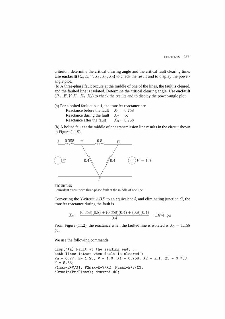
CONTENTS 257
criterion, determine the critical clearing angle and the critical fault clearing time.Useeacfault(Pm, E, V,X1, X2, X3) to check the result and to display the power-angle plot.(b) A three-phase fault occurs at the middle of one of the lines, the fault is cleared,and the faulted line is isolated. Determine the critical clearing angle. Useeacfault(Pm, E, V, X1, X2, X3) to check the results and to display the power-angle plot.
(a) For a bolted fault at bus 1, the transfer reactance areReactance before the faultX1 = 0.758Reactance during the faultX2 = ∞Reactance after the fault X3 = 0.758
(b) A bolted fault at the middle of one transmission line results in the circuit shownin Figure (11.5).
....................................
..................................................
.............. ....................................
..................................................
...........................................................................................................
............................
.........
...............................................................
..........................................................................................................................................................................................
....................................................................................................
.............................................................................................
µ´¶³
µ´¶³
A 0.358 C 0.8 B
∞ V = 1.0
F
0.4 0.4E′
FIGURE 95Equivalent circuit with three-phase fault at the middle of one line.
Converting the Y-circuitABF to an equivalentδ, and eliminating junctionC, thetransfer reactance during the fault is
X2 =(0.358)(0.8) + (0.358)(0.4) + (0.8)(0.4)
0.4= 1.874 pu
From Figure (11.2), the reactance when the faulted line is isolated isX3 = 1.158pu.
We use the following commands
disp(’(a) Fault at the sending end, ...both lines intact when fault is cleared’)Pm = 0.77; E= 1.25; V = 1.0; X1 = 0.758; X2 = inf; X3 = 0.758;H = 5.66;P1max=E*V/X1; P2max=E*V/X2; P3max=E*V/X3;d0=asin(Pm/P1max); dmax=pi-d0;
258 CONTENTS
dc=acos((Pm*(dmax-d0)+P3max*cos(dmax)-P2max*cos(d0))/ ...(P3max-P2max));dcdeg=dc*180/pi;disp([’Critical clearing angle = ’, num2str(dcdeg)])tc = sqrt(2*H*(dc-d0)/(pi*60*Pm));disp([’Critical clearing time = ’, num2str(tc)])% Check using eacfaulteacfault(Pm, E, V, X1, X2, X3)
disp(’(b) Fault at the mid-point of one line, ....faulted line is isolated’)X2 = 1.874; X3 = 1.158;eacfault(Pm, E, V, X1, X2, X3)
which result in
(a) Fault at the sending end,both lines intact when fault is cleared
Critical clearing angle = 82.5927Critical clearing time = 0.27302
For this case tc can be found from analytical formula.To find tc enter Inertia Constant H, (or 0 to skip) H = 5.66
Initial power angle = 27.835Maximum angle swing = 152.165Critical clearing angle = 82.593
Critical clearing time = 0.273 sec.Current plot held
(b) Fault at the mid-point of one line,faulted line is isolated
Initial power angle = 27.835Maximum angle swing = 134.494Critical clearing angle = 77.817
11.16.The machine of Problem 11.6 is delivering a real power input of 0.77 perunit to the infinite bus at a voltage of 1.0 per unit. The generator excitation voltageis E′ = 1.25 per unit. A three-phase fault at the middle of one line is cleared byisolating the faulted circuit simultaneously at both ends.(a) The fault is cleared in 0.2 second. Obtain the numerical solution of the swingequation for 1.5 seconds. Select one of the functionsswingmeu, swingrk2, orswingrk4.

CONTENTS 259
(b) Repeat the simulation and obtain the swing plots when fault is cleared in 0.4second, and for the critical clearing time.
The reactances between the generator internal emf and the infinite bus calculatedin Problem 11.15 are:X1 = 0.758, X2 = 1.874, andX3 = 1.158. The swingcurves are obtained for fault clearing times oftc = 0.2, tc = 0.4, andtc = 0.37,with swingmeufunction. We use the following statements.
global Pm f H E V X1 X2 X3Pm = 0.770; E = 1.25; V = 1.0;X1 = 0.758; X2 = 1.874; X3 = 1.158;H = 5.66; f = 60; tf = 1.5; Dt = 0.01;% (a) Fault is cleared in 0.3 sec.tc = 0.2;swingmeu(Pm, E, V, X1, X2, X3, H, f, tc, tf, Dt)% (b) Fault is cleared in 0.4 sec.tc = .4;swingmeu(Pm, E, V, X1, X2, X3, H, f, tc, tf, Dt)tc = .37;swingmeu(Pm, E, V, X1, X2, X3, H, f, tc, tf, Dt)
Run the program to obtain the swing curves.
Critical clearing time = 0.37 secondsCritical clearing angle = 77.82 degrees
11.17.Consider the power system network of Example 11.7 with the described op-erating condition. A three-phase fault occurs on line 1–5 near bus 5 and is clearedby the simultaneous opening of breakers at both ends of the line. Using thetrstabprogram, perform a transient stability analysis. Determine the system stability for
(a) When the fault is cleared in 0.2 second(b) When the fault is cleared in 0.4 second(c) Repeat the simulation to determine the critical clearing time.
Run Example 11.7 for fault at bus 5 to obtain the swing plots fortc = 0.2, andtc = 0.4. Repeat until the critical clearing timetc = 0.34 second is obtained.
11.18.The power system network of an electric company is shown in Figure 96.
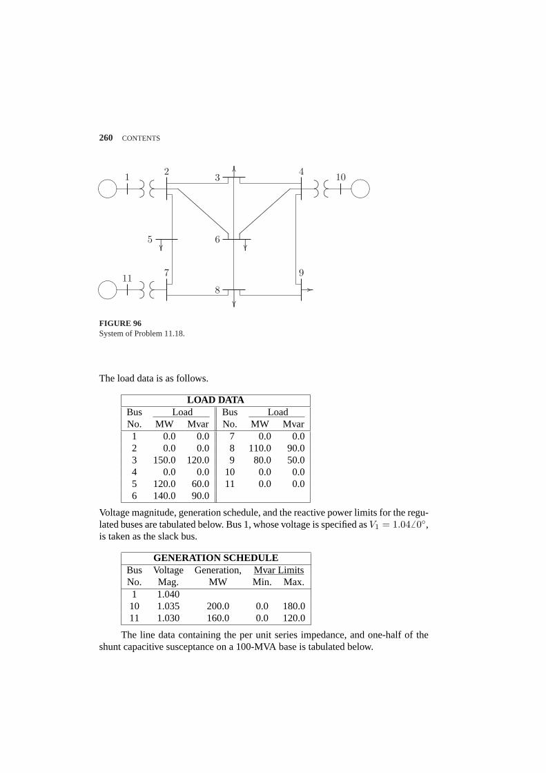
260 CONTENTS
µ´¶³
.......................................................................... .......................................................................... ...............
........
................................................... .......................................................................... µ´
¶³.........................................................................................................................................................................................................
.........................................................................................................................................................................................................
µ´¶³
.......................................................................... ..........................................................................
........
........
........
.......................
................
.......................................
........
........
.......................................................................
.......................................................
........
........
........
............................................... ................
1 2 3 4 10
5 6
7
8
911
FIGURE 96System of Problem 11.18.
The load data is as follows.
LOAD DATABus Load Bus LoadNo. MW Mvar No. MW Mvar1 0.0 0.0 7 0.0 0.02 0.0 0.0 8 110.0 90.03 150.0 120.0 9 80.0 50.04 0.0 0.0 10 0.0 0.05 120.0 60.0 11 0.0 0.06 140.0 90.0
Voltage magnitude, generation schedule, and the reactive power limits for the regu-lated buses are tabulated below. Bus 1, whose voltage is specified asV1 = 1.04 6 0,is taken as the slack bus.
GENERATION SCHEDULEBus Voltage Generation, Mvar LimitsNo. Mag. MW Min. Max.1 1.04010 1.035 200.0 0.0 180.011 1.030 160.0 0.0 120.0
The line data containing the per unit series impedance, and one-half of theshunt capacitive susceptance on a 100-MVA base is tabulated below.
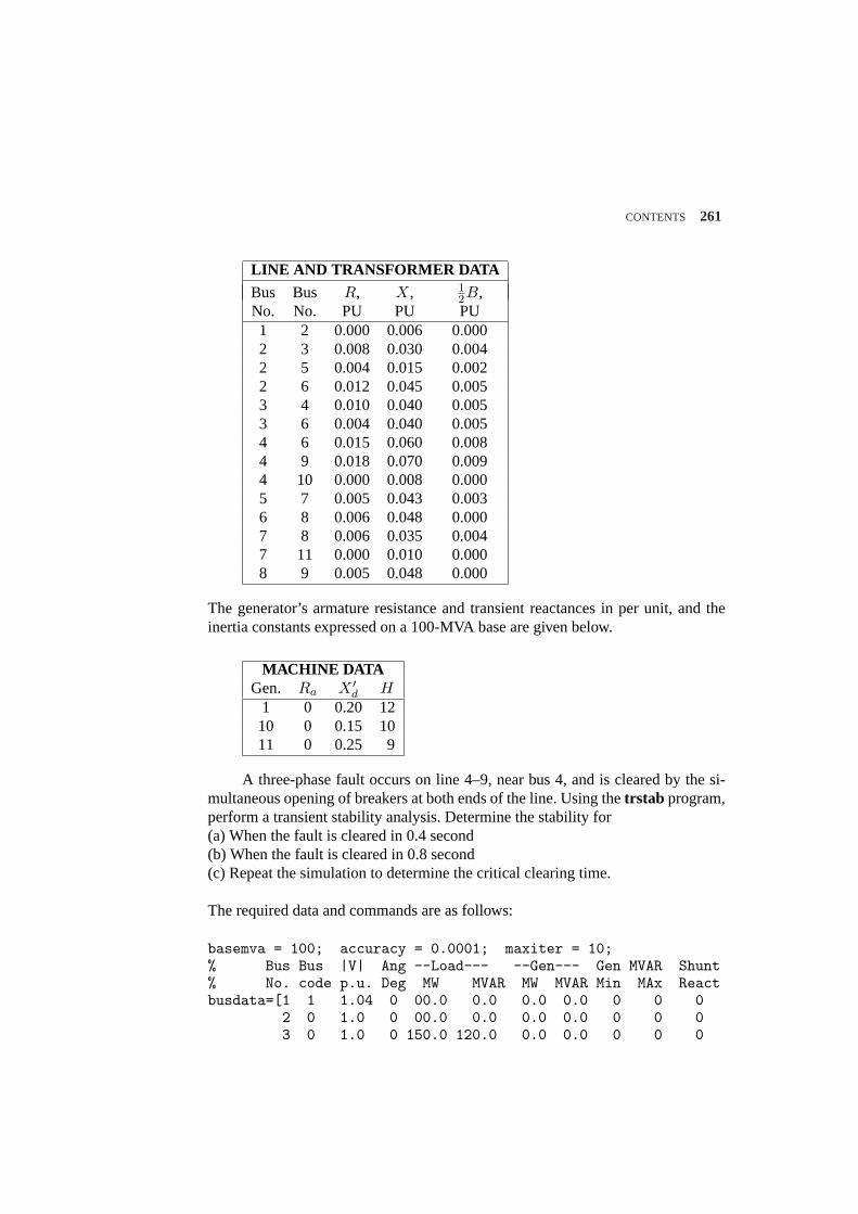
CONTENTS 261
LINE AND TRANSFORMER DATABus Bus R, X, 1
2B,No. No. PU PU PU1 2 0.000 0.006 0.0002 3 0.008 0.030 0.0042 5 0.004 0.015 0.0022 6 0.012 0.045 0.0053 4 0.010 0.040 0.0053 6 0.004 0.040 0.0054 6 0.015 0.060 0.0084 9 0.018 0.070 0.0094 10 0.000 0.008 0.0005 7 0.005 0.043 0.0036 8 0.006 0.048 0.0007 8 0.006 0.035 0.0047 11 0.000 0.010 0.0008 9 0.005 0.048 0.000
The generator’s armature resistance and transient reactances in per unit, and theinertia constants expressed on a 100-MVA base are given below.
MACHINE DATAGen. Ra X ′
d H1 0 0.20 1210 0 0.15 1011 0 0.25 9
A three-phase fault occurs on line 4–9, near bus 4, and is cleared by the si-multaneous opening of breakers at both ends of the line. Using thetrstab program,perform a transient stability analysis. Determine the stability for(a) When the fault is cleared in 0.4 second(b) When the fault is cleared in 0.8 second(c) Repeat the simulation to determine the critical clearing time.
The required data and commands are as follows:
basemva = 100; accuracy = 0.0001; maxiter = 10;% Bus Bus |V| Ang --Load--- --Gen--- Gen MVAR Shunt% No. code p.u. Deg MW MVAR MW MVAR Min MAx Reactbusdata=[1 1 1.04 0 00.0 0.0 0.0 0.0 0 0 0
2 0 1.0 0 00.0 0.0 0.0 0.0 0 0 03 0 1.0 0 150.0 120.0 0.0 0.0 0 0 0
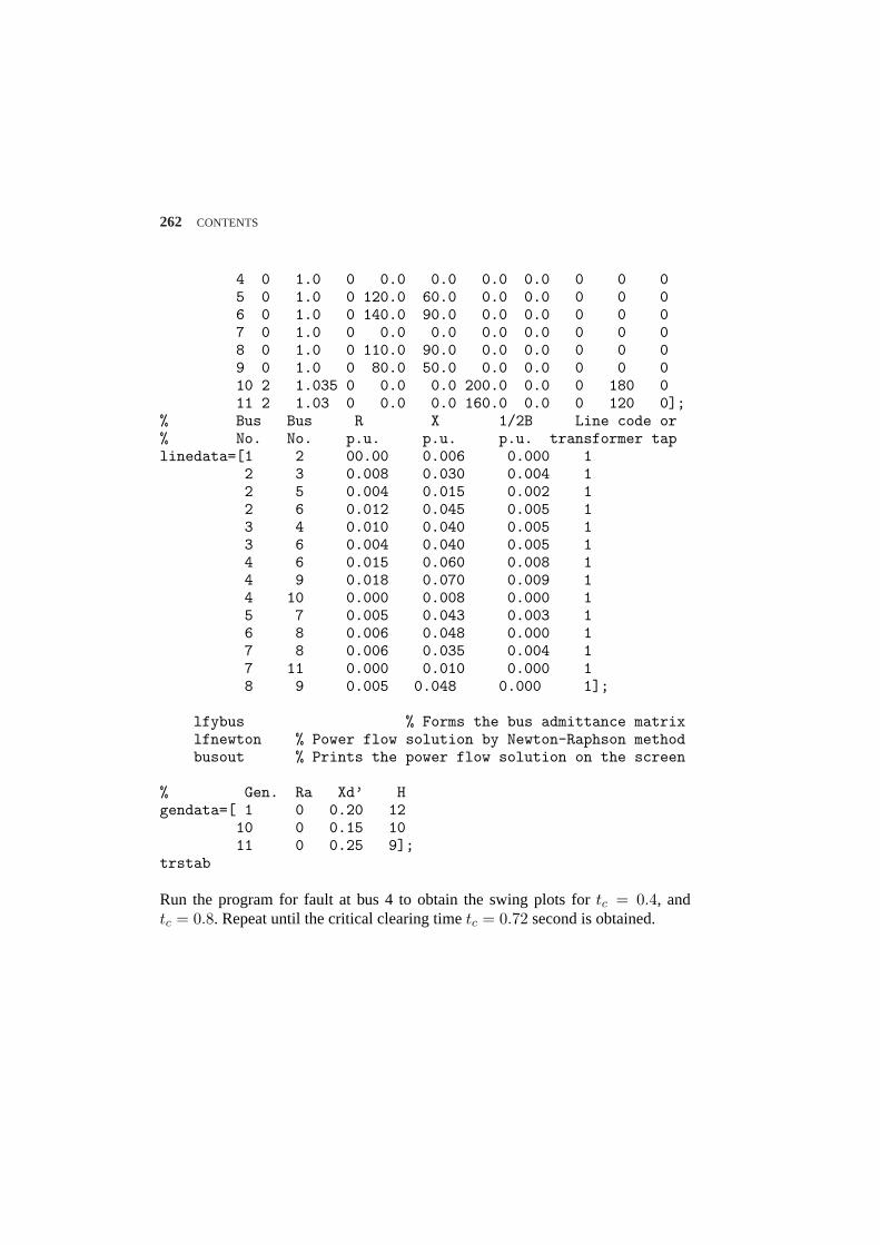
262 CONTENTS
4 0 1.0 0 0.0 0.0 0.0 0.0 0 0 05 0 1.0 0 120.0 60.0 0.0 0.0 0 0 06 0 1.0 0 140.0 90.0 0.0 0.0 0 0 07 0 1.0 0 0.0 0.0 0.0 0.0 0 0 08 0 1.0 0 110.0 90.0 0.0 0.0 0 0 09 0 1.0 0 80.0 50.0 0.0 0.0 0 0 010 2 1.035 0 0.0 0.0 200.0 0.0 0 180 011 2 1.03 0 0.0 0.0 160.0 0.0 0 120 0];
% Bus Bus R X 1/2B Line code or% No. No. p.u. p.u. p.u. transformer taplinedata=[1 2 00.00 0.006 0.000 1
2 3 0.008 0.030 0.004 12 5 0.004 0.015 0.002 12 6 0.012 0.045 0.005 13 4 0.010 0.040 0.005 13 6 0.004 0.040 0.005 14 6 0.015 0.060 0.008 14 9 0.018 0.070 0.009 14 10 0.000 0.008 0.000 15 7 0.005 0.043 0.003 16 8 0.006 0.048 0.000 17 8 0.006 0.035 0.004 17 11 0.000 0.010 0.000 18 9 0.005 0.048 0.000 1];
lfybus % Forms the bus admittance matrixlfnewton % Power flow solution by Newton-Raphson methodbusout % Prints the power flow solution on the screen
% Gen. Ra Xd’ Hgendata=[ 1 0 0.20 12
10 0 0.15 1011 0 0.25 9];
trstab
Run the program for fault at bus 4 to obtain the swing plots fortc = 0.4, andtc = 0.8. Repeat until the critical clearing timetc = 0.72 second is obtained.
CHAPTER 12 PROBLEMS
12.1.A 250-MW, 60-Hz turbine generator set has a speed regulation of 5 percentbased on its own rating. The generator frequency decreases from 60 Hz to a steadystate value of 59.7Hz. Determine the increase in the turbine power output.
The change in the angular frequency is
∆ω =59.7− 60
60= −0.005 pu
From (12.7), the change in the turbine power output is
∆Pg = − 1R
∆ω = (− 10.05
)(−0.005) = 0.10 pu
= 25 MW
12.2.Two generating units rated for 250 MW and 400 MW have governor speedregulation of 6.0 and 6.4 percent, respectively, from no-load to full-load, respec-tively. They are operating in parallel and share a load of 500 MW. Assuming freegovernor action, determine the load shared by each unit.
Expressing the governor speed regulation of each unit to a common MVA base of1000, we get
R1 =1000250
(0.06) = 0.24
R2 =1000400
(0.064) = 0.16
Since both units are operating at the same frequency, from (12.7) we have
R1Pg1 = R2Pg2
263
264 CONTENTS
or
Pg2 =R1
R2Pg1 =
0.240.16
Pg1 = 1.5Pg1
Also
Pg1 + Pg2 = PD
Substituting forPg2 in the above equation, we have
Pg1 + 1.5Pg1 =5001000
which result in
Pg1 =0.52.5
= 0.2 pu or 200 MW
Pg2 = (1.5)(0.2) = 0.3 pu or 300 MW
12.3.A single area consists of two generating units, rated at 400 and 800 MVA,with speed regulation of 4 percent and 5 percent on their respective ratings. Theunits are operating in parallel, sharing 700 MW. Unit 1 supplies 200 MW and unit2 supplies 500 MW at 1.0 per unit (60 Hz) frequency. The load is increased by 130MW.(a) Assume there is no frequency-dependent load, i.e.,D = 0. Find the steady-statefrequency deviation and the new generation on each unit.(b) The load varies 0.804 percent for every 1 percent change in frequency, i.e.,D = 0.804. Find the steady-state frequency deviation and the new generation oneach unit.
Express the governor speed regulation of each unit to a common 1000MVA base,we have
R1 =1000400
(0.04) = 0.1 pu
R2 =1000800
(0.05) = 0.0625 pu
The per unit load change is
∆PL =1301000
= 0.13 pu
CONTENTS 265
(a) From (12.15) withD = 0, the per unit steady-state frequency deviation is
∆ωss =−∆PL1
R1+ 1
R2
=−0.13
10 + 16= −0.005 pu
Thus, the steady-state frequency deviation in Hz is
∆f = (−0.005)(60) = −0.30 Hz
and the new frequency is
f = f0 + ∆f = 60− 0.30 = 59.70 Hz
The change in generation for each unit is
∆P1 = −∆ω
R1= −−0.005
0.10= 0.05 pu
= 50 MW
∆P2 = −∆ω
R2= −−0.005
0.0625= 0.08 pu
= 80 MW
Thus, unit 1 supplies 250 MW and unit 2 supplies 580 MW at the new operatingfrequency of59.70 Hz.
(b) ForD = 0.804, the per unit steady-state frequency deviation is
∆ωss =−∆PL
1R1
+ 1R2
+ D=
−0.1310 + 16 + 0.804
= −0.00485 pu
Thus, the steady-state frequency deviation in Hz is
∆f = (−0.00485)(60) = −0.291 Hz
and the new frequency is
f = f0 + ∆f = 60− 0.291 = 59.709 Hz
The change in generation for each unit is
∆P1 = −∆ω
R1= −−0.00485
0.1= 0.0485 pu
= 48.5 MW
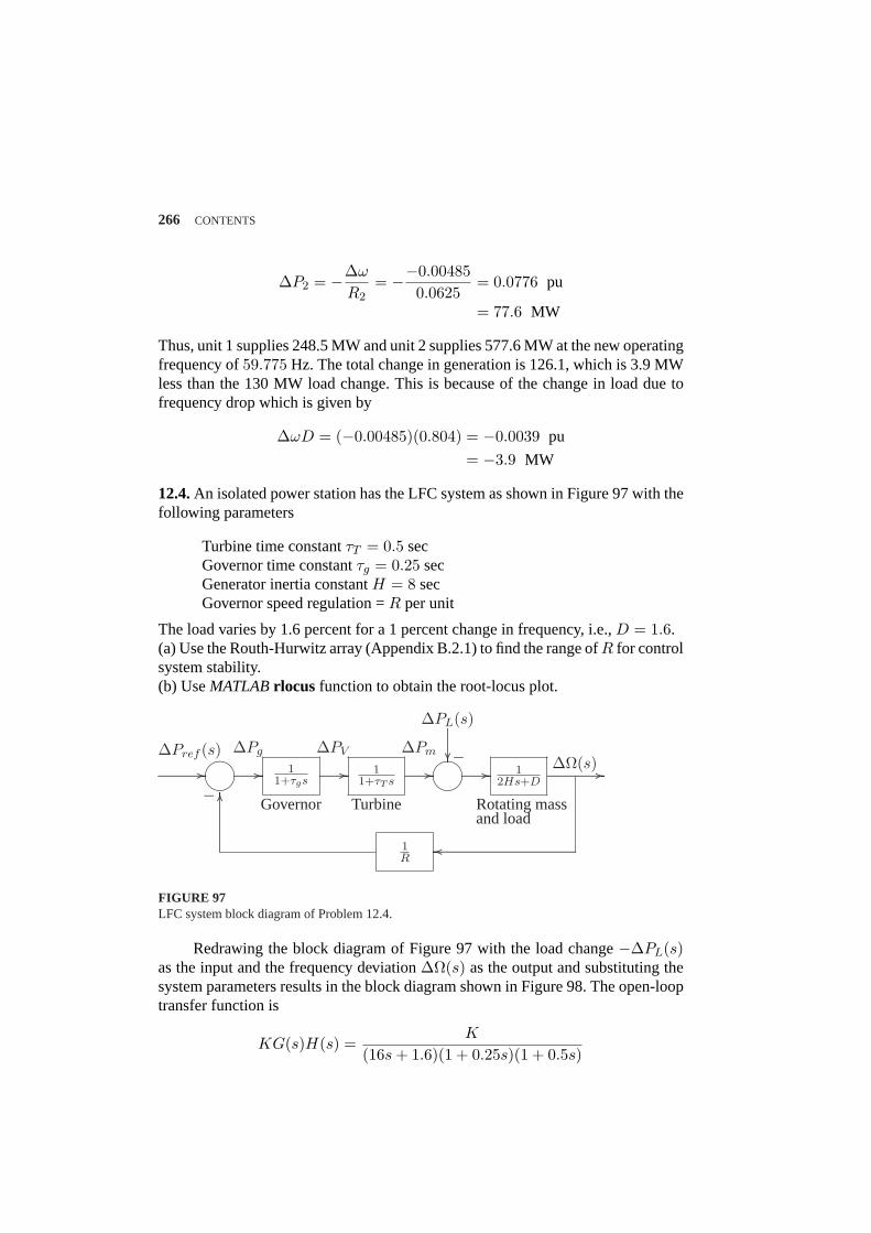
266 CONTENTS
∆P2 = −∆ω
R2= −−0.00485
0.0625= 0.0776 pu
= 77.6 MW
Thus, unit 1 supplies 248.5 MW and unit 2 supplies 577.6 MW at the new operatingfrequency of59.775 Hz. The total change in generation is 126.1, which is 3.9 MWless than the 130 MW load change. This is because of the change in load due tofrequency drop which is given by
∆ωD = (−0.00485)(0.804) = −0.0039 pu
= −3.9 MW
12.4.An isolated power station has the LFC system as shown in Figure 97 with thefollowing parameters
Turbine time constantτT = 0.5 secGovernor time constantτg = 0.25 secGenerator inertia constantH = 8 secGovernor speed regulation =R per unit
The load varies by 1.6 percent for a 1 percent change in frequency, i.e.,D = 1.6.(a) Use the Routh-Hurwitz array (Appendix B.2.1) to find the range ofR for controlsystem stability.(b) UseMATLABrlocus function to obtain the root-locus plot.
.................................................................................................. ................
µ´¶³
................................................................. ................ ................................................................. ................ ................................................................. ................
µ´¶³
................................................................. ................ .................................................................................................................. ................
..........................................................................................................................................................................................................................................................................................................................................................................................................................
11+τgs
11+τT s
12Hs+D
1R
∆Pref (s)
−
∆PV∆Pg ∆Pm
.................................................................
........
........
........
∆PL(s)
−
Governor Turbine Rotating massand load
∆Ω(s)
FIGURE 97LFC system block diagram of Problem 12.4.
Redrawing the block diagram of Figure 97 with the load change−∆PL(s)as the input and the frequency deviation∆Ω(s) as the output and substituting thesystem parameters results in the block diagram shown in Figure 98. The open-looptransfer function is
KG(s)H(s) =K
(16s + 1.6)(1 + 0.25s)(1 + 0.5s)
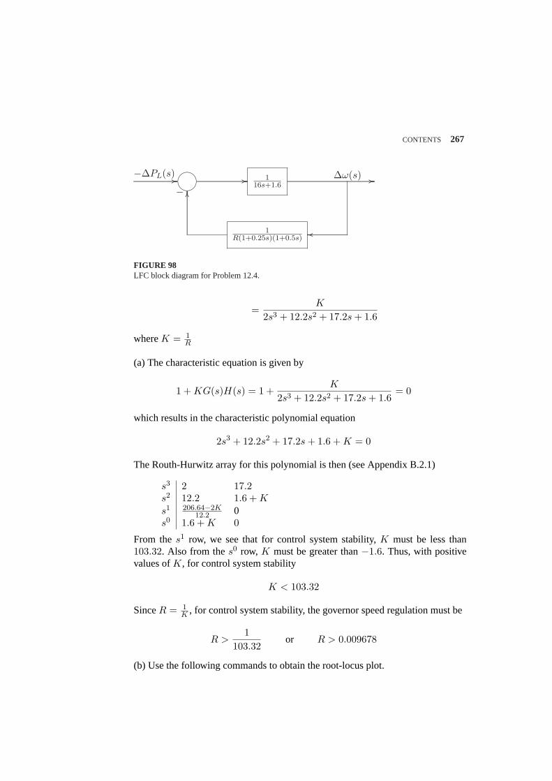
CONTENTS 267
...................................................................................................................................... ................
µ´¶³
........................................................................................................................................................ ................ ........................................................................................................................................................................................................................................................... ................
...................................................................................................................................................................................................................................................................................................
116s+1.6
1R(1+0.25s)(1+0.5s)
−∆PL(s)
−∆ω(s)
FIGURE 98LFC block diagram for Problem 12.4.
=K
2s3 + 12.2s2 + 17.2s + 1.6
whereK = 1R
(a) The characteristic equation is given by
1 + KG(s)H(s) = 1 +K
2s3 + 12.2s2 + 17.2s + 1.6= 0
which results in the characteristic polynomial equation
2s3 + 12.2s2 + 17.2s + 1.6 + K = 0
The Routh-Hurwitz array for this polynomial is then (see Appendix B.2.1)
s3 2 17.2s2 12.2 1.6 + Ks1 206.64−2K
12.2 0s0 1.6 + K 0
From thes1 row, we see that for control system stability,K must be less than103.32. Also from thes0 row, K must be greater than−1.6. Thus, with positivevalues ofK, for control system stability
K < 103.32
SinceR = 1K , for control system stability, the governor speed regulation must be
R >1
103.32or R > 0.009678
(b) Use the following commands to obtain the root-locus plot.
268 CONTENTS
num=1;den = [2 12.2 170.2 1.6];figure(1), rlocus(num, den)
12.5.The governor speed regulation of Problem 12.4 is set toR = 0.04 per unit.The turbine rated output is200 MW at nominal frequency of60 Hz. A sudden loadchange of50 MW (∆PL = 0.25 per unit) occurs.(a) Find the steady-state frequency deviation in Hz.(b) Obtain the closed-loop transfer function and useMATLAB to obtain the fre-quency deviation step response.(c) Construct theSIMULINKblock diagram and obtain the frequency deviation re-sponse.
The closed-loop transfer function of the system shown in Figure 98 is
∆Ω(s)−∆PL(s)
= T (s) =(1 + 0.25s)(1 + 0.5s)
(16s + 1.6)(1 + 0.25s)(1 + 0.5s) + 1/.04
=0.0625s2 + 0.375s + 0.5s3 + 6.1s2 + 8.6s + 13.3
(a) The steady-state frequency deviation due to a step input is
∆ωss = lims→0
s∆Ω(s) =0.513.3
(−0.25) = −0.0093985 pu
= −0.5639 Hz
(b) Use the following commands to obtain the step response.
PL = 0.25;numc = [0.0625 0.375 0.5];denc = [1 6.1 8.6 13.3];t = 0:.02:10; c = -PL*step(num, den, t);figure(2), plot(t, c), xlabel(’t, sec’), ylabel(’pu’)title(’Frequency deviation step response’), grid
(c) Change the parameters of theSIMULINK modelsim12ex1.mdlaccording tothe values given in Problem 12.4 and run in theSIMULINK window to obtain theresponse.12.6.The LFC system in Problem 12.5 is equipped with the secondary integralcontrol loop for automatic generation control as shown in Figure 12.16 (Text).(a) Use theMATLABstepfunction to obtain the frequency deviation step responsefor a sudden load change of∆PL = 0.25 per unit. Set the integral controller gainto KI = 9.
CONTENTS 269
(b) Construct theSIMULINKblock diagram and obtain the frequency deviation re-sponse for the condition in part (a).
(a) Substituting for the system parameters in (12.16), with speed regulation ad-justed toR = 0.04 per unit, results in the following closed-loop transfer function
T (s) =0.0625s3 + 0.375s2 + 0.5s
s4 + 6.1s3 + 8.6s2 + 13.3s + 0.5KI
Use the following commands to obtain the step response.
PL = 0.25;KI = 9;num = [0.0625 0.375 0.5 0];den = [1 6.1 8.6 13.3 0.5*KI];t = 0:.02:12;c = -PL*step(num, den, t);plot(t, c), gridxlabel(’t, sec’), ylabel(’pu’)title(’Frequency deviation step response’)
(b) Change the parameters of theSIMULINK modelsim12ex3.mdlaccording tothe values given in Problem 12.4 and run in theSIMULINK window to obtain theresponse.
12.7.The load changes of 200 MW and 150 MW occur simultaneously in areas 1and 2 of the two-area system of Example 12.4. Modify theSIMULINK block dia-gramsim12ex4.mdl, and obtain the frequency and power deviation responses.
Apply the above load changes to theSIMULINK block diagramsim12ex4.mdl,and obtain the frequency deviation and the power responses (sim12p7.mdl).
12.8.Modify theSIMULINKmodel for the two-area system of Example 12.5 withthe tie-line bias control (sim12ex5.mdl) to include the load changes specified inProblem 12.7. Obtain the frequency and power response deviation for each area.
Apply the load changes specified in Problem 12.7 to theSIMULINK block dia-gram (sim12ex5.mdl), and obtain the frequency and power deviation responses(sim12p8.mdl).
12.9.A generating unit has a simplified linearized AVR system as shown in Figure99.(a) Use the Routh-Hurwitz array (Appendix B.2.1) to find the range ofKA for
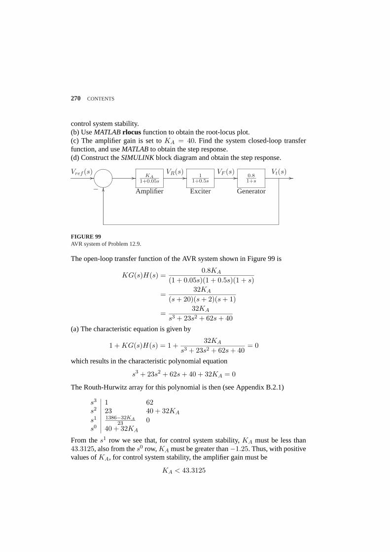
270 CONTENTS
control system stability.(b) UseMATLABrlocus function to obtain the root-locus plot.(c) The amplifier gain is set toKA = 40. Find the system closed-loop transferfunction, and useMATLABto obtain the step response.(d) Construct theSIMULINKblock diagram and obtain the step response.
......................................................................................................... ................
½¼
¾»......................................................................................................... ................
Amplifier
......................................................................................................... ................
Exciter
......................................................................................................... ................
Generator
........................................................................................................................... ................
........
........
........
........
........
........
........
........
........
........
........
........
........
........
........
........
........
......................
................
KA1+0.05s
11+0.5s
0.81+s
Vref (s)
−
VR(s) VF (s) Vt(s)
FIGURE 99AVR system of Problem 12.9.
The open-loop transfer function of the AVR system shown in Figure 99 is
KG(s)H(s) =0.8KA
(1 + 0.05s)(1 + 0.5s)(1 + s)
=32KA
(s + 20)(s + 2)(s + 1)
=32KA
s3 + 23s2 + 62s + 40(a) The characteristic equation is given by
1 + KG(s)H(s) = 1 +32KA
s3 + 23s2 + 62s + 40= 0
which results in the characteristic polynomial equation
s3 + 23s2 + 62s + 40 + 32KA = 0
The Routh-Hurwitz array for this polynomial is then (see Appendix B.2.1)
s3 1 62s2 23 40 + 32KA
s1 1386−32KA23 0
s0 40 + 32KA
From thes1 row we see that, for control system stability,KA must be less than43.3125, also from thes0 row,KA must be greater than−1.25. Thus, with positivevalues ofKA, for control system stability, the amplifier gain must be
KA < 43.3125
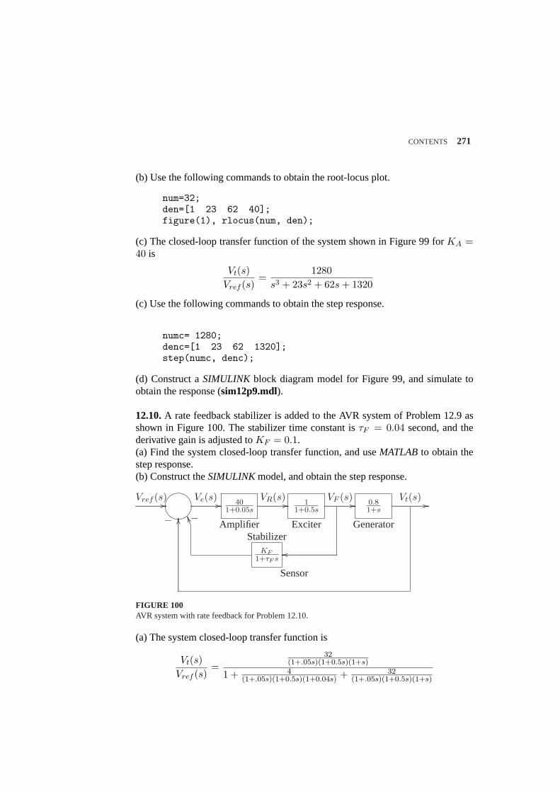
CONTENTS 271
(b) Use the following commands to obtain the root-locus plot.
num=32;den=[1 23 62 40];figure(1), rlocus(num, den);
(c) The closed-loop transfer function of the system shown in Figure 99 forKA =40 is
Vt(s)Vref (s)
=1280
s3 + 23s2 + 62s + 1320
(c) Use the following commands to obtain the step response.
numc= 1280;denc=[1 23 62 1320];step(numc, denc);
(d) Construct aSIMULINK block diagram model for Figure 99, and simulate toobtain the response (sim12p9.mdl).
12.10.A rate feedback stabilizer is added to the AVR system of Problem 12.9 asshown in Figure 100. The stabilizer time constant isτF = 0.04 second, and thederivative gain is adjusted toKF = 0.1.(a) Find the system closed-loop transfer function, and useMATLABto obtain thestep response.(b) Construct theSIMULINKmodel, and obtain the step response.
.................................................................................................. ................
½¼
¾».................................................................................................. ................ .................................................................................................. ................ .................................................................................................. ................ .................................................................................................................. ................
........
........
........
........
........
........
........
........
........
........
........
........
........
........
........
........
........
........
........
........
........
........
........
........
....................
................
401+0.05s
11+0.5s
0.81+s
Vref (s)
−
Ve(s) VR(s) VF (s) Vt(s)
Amplifier Exciter Generator
Sensor
...................................................................................................................................................................................KF
1+τF s
......................................................
Stabilizer
−
FIGURE 100AVR system with rate feedback for Problem 12.10.
(a) The system closed-loop transfer function is
Vt(s)Vref (s)
=32
(1+.05s)(1+0.5s)(1+s)
1 + 4(1+.05s)(1+0.5s)(1+0.04s) + 32
(1+.05s)(1+0.5s)(1+s)
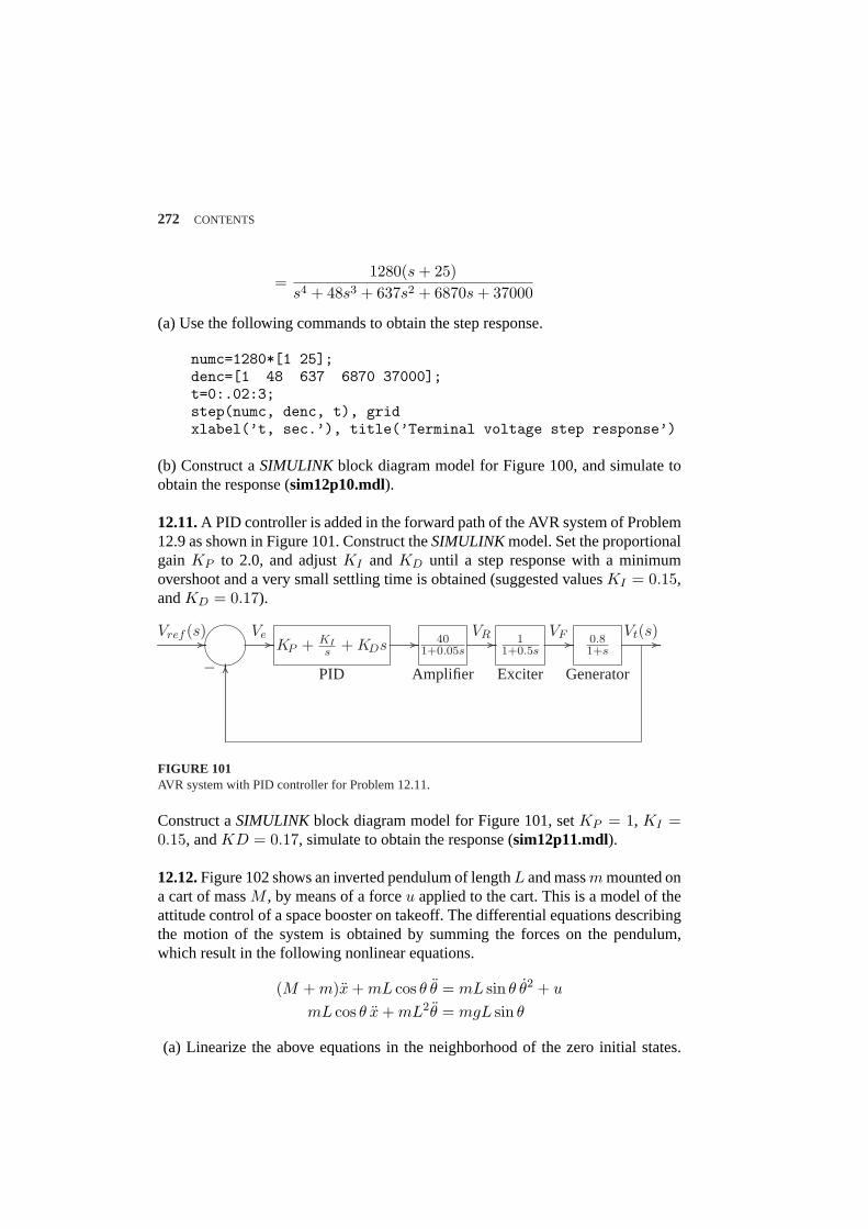
272 CONTENTS
=1280(s + 25)
s4 + 48s3 + 637s2 + 6870s + 37000
(a) Use the following commands to obtain the step response.
numc=1280*[1 25];denc=[1 48 637 6870 37000];t=0:.02:3;step(numc, denc, t), gridxlabel(’t, sec.’), title(’Terminal voltage step response’)
(b) Construct aSIMULINK block diagram model for Figure 100, and simulate toobtain the response (sim12p10.mdl).
12.11.A PID controller is added in the forward path of the AVR system of Problem12.9 as shown in Figure 101. Construct theSIMULINKmodel. Set the proportionalgain KP to 2.0, and adjustKI and KD until a step response with a minimumovershoot and a very small settling time is obtained (suggested valuesKI = 0.15,andKD = 0.17).
.................................................................................................... ................
½¼
¾».................................................................. ................ .................................................................. ................ .................................................................. ................ .................................................................. ................ ................................................................................... ................
........
........
........
........
........
........
........
........
........
........
........
........
........
........
........
........
.....................
................
KP + KIs + KDs 40
1+0.05s1
1+0.5s0.81+s
Vref (s)
−
Ve VR VF Vt(s)
PID Amplifier Exciter Generator
FIGURE 101AVR system with PID controller for Problem 12.11.
Construct aSIMULINK block diagram model for Figure 101, setKP = 1, KI =0.15, andKD = 0.17, simulate to obtain the response (sim12p11.mdl).
12.12.Figure 102 shows an inverted pendulum of lengthL and massm mounted ona cart of massM , by means of a forceu applied to the cart. This is a model of theattitude control of a space booster on takeoff. The differential equations describingthe motion of the system is obtained by summing the forces on the pendulum,which result in the following nonlinear equations.
(M + m)x + mL cos θ θ = mL sin θ θ2 + u
mL cos θ x + mL2θ = mgL sin θ
(a) Linearize the above equations in the neighborhood of the zero initial states.
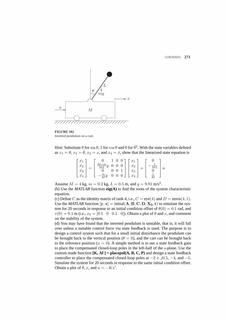
CONTENTS 273
...................
......................................
m m
......................................................................................... ................u
......................................................................................... ................ x
.............................................
........
........
........
mg
L
..................................
θ
M
....................................................................................................................................................................................................................................................................................................................................................................................................................................................................................................................................................................................................................................................................................................
.........................................................................................................................................................................................
.........................................................................................................................................................................................
.........................................................................................................................................................................................
FIGURE 102Inverted pendulum on a cart.
Hint: Substituteθ for sin θ, 1 for cos θ and 0 forθ2. With the state variables definedasx1 = θ, x2 = θ, x3 = x, andx4 = x, show that the linearized state equation is
x1
x2
x3
x4
=
0 1 0 0M+mML g 0 0 0
0 0 0 1−m
M g 0 0 0
x1
x2
x3
x4
+
0− 1
ML01M
u
AssumeM = 4 kg, m = 0.2 kg, L = 0.5 m, andg = 9.81 m/s2.(b) Use theMATLABfunctioneig(A) to find the roots of the system characteristicequation.(c) DefineC as the identity matrix of rank 4, i.e.,C = eye(4) andD = zeros(4, 1).Use theMATLABfunction[y,x] = initial(A,B,C,D,X0, t) to simulate the sys-tem for 20 seconds in response to an initial condition offset ofθ(0) = 0.1 rad, andx(0) = 0.1 m (i.e.,x0 = [0.1 0 0.1 0]). Obtain a plot ofθ andx, and commenton the stability of the system.(d) You may have found that the inverted pendulum is unstable, that is, it will fallover unless a suitable control force via state feedback is used. The purpose is todesign a control system such that for a small initial disturbance the pendulum canbe brought back to the vertical position (θ = 0), and the cart can be brought backto the reference position (x = 0). A simple method is to use a state feedback gainto place the compensated closed-loop poles in the left-half of thes-plane. Use thecustom made function[K, Af ] = placepol(A, B, C, P) and design a state feedbackcontroller to place the compensated closed-loop poles at−2 ± j0.5, −4, and−5.Simulate the system for 20 seconds in response to the same initial condition offset.Obtain a plot ofθ, x, andu = −Kx′.
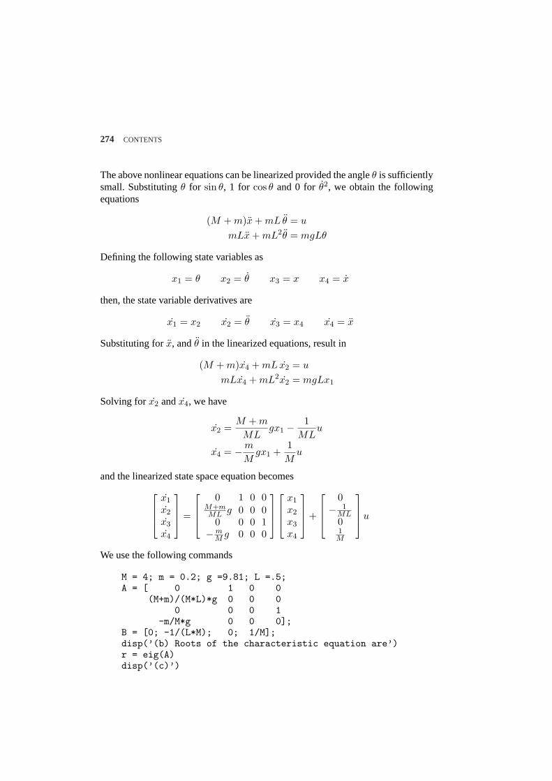
274 CONTENTS
The above nonlinear equations can be linearized provided the angleθ is sufficientlysmall. Substitutingθ for sin θ, 1 for cos θ and 0 forθ2, we obtain the followingequations
(M + m)x + mL θ = u
mLx + mL2θ = mgLθ
Defining the following state variables as
x1 = θ x2 = θ x3 = x x4 = x
then, the state variable derivatives are
x1 = x2 x2 = θ x3 = x4 x4 = x
Substituting forx, andθ in the linearized equations, result in
(M + m)x4 + mL x2 = u
mLx4 + mL2x2 = mgLx1
Solving forx2 andx4, we have
x2 =M + m
MLgx1 − 1
MLu
x4 = −m
Mgx1 +
1M
u
and the linearized state space equation becomes
x1
x2
x3
x4
=
0 1 0 0M+mML g 0 0 0
0 0 0 1−m
M g 0 0 0
x1
x2
x3
x4
+
0− 1
ML01M
u
We use the following commands
M = 4; m = 0.2; g =9.81; L =.5;A = [ 0 1 0 0
(M+m)/(M*L)*g 0 0 00 0 0 1
-m/M*g 0 0 0];B = [0; -1/(L*M); 0; 1/M];disp(’(b) Roots of the characteristic equation are’)r = eig(A)disp(’(c)’)
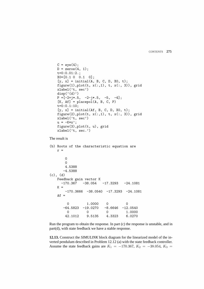
CONTENTS 275
C = eye(4);D = zeros(4, 1);t=0:0.01:2.;X0=[0.1 0 0.1 0];[y, x] = initial(A, B, C, D, X0, t);figure(1),plot(t, x(:,1), t, x(:, 3)), gridxlabel(’t, sec’)disp(’(d)’)P =[-2+j*.5, -2-j*.5, -5, -4];[K, Af] = placepol(A, B, C, P)t=0:0.1:10;[y, x] = initial(Af, B, C, D, X0, t);figure(2),plot(t, x(:,1), t, x(:, 3)), gridxlabel(’t, sec’)u = -K*x’;figure(3),plot(t, u), gridxlabel(’t, sec.’)
The result is
(b) Roots of the characteristic equation arer =
004.5388
-4.5388(c), (d)
Feedback gain vector K-170.367 -38.054 -17.3293 -24.1081
K =-170.3666 -38.0540 -17.3293 -24.1081
Af =
0 1.0000 0 0-64.5823 -19.0270 -8.6646 -12.05400 0 0 1.000042.1012 9.5135 4.3323 6.0270
Run the program to obtain the response. In part (c) the response is unstable, and inpart(d), with state feedback we have a stable response.
12.13.Construct theSIMULINK block diagram for the linearized model of the in-verted pendulum described in Problem 12.12 (a) with the state feedback controller.Assume the state feedback gains areK1 = −170.367, K2 = −38.054, K3 =
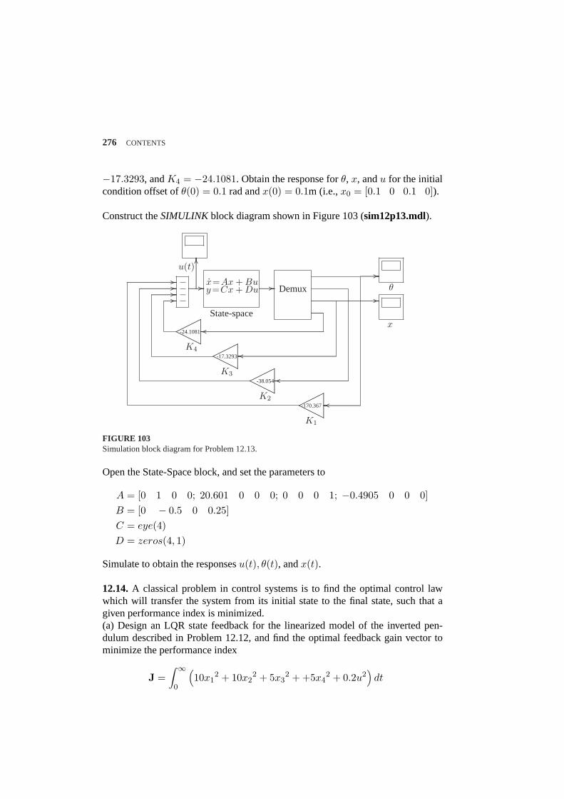
276 CONTENTS
−17.3293, andK4 = −24.1081. Obtain the response forθ, x, andu for the initialcondition offset ofθ(0) = 0.1 rad andx(0) = 0.1m (i.e.,x0 = [0.1 0 0.1 0]).
Construct theSIMULINKblock diagram shown in Figure 103 (sim12p13.mdl).
................................................................................................................................................... ................ −−−−......................................................... ........................
........
........
........
........
........
........
........
........
........
..................
................u(t)
x=Ax + Buy=Cx + Du
State-space
......................................................... ................ Demux
....................................................................................................................................................................
..................................
.........................................................................................................
..................................
.....
......................................................................................................................................................................................................................................................................................................................................................................
.....................................................................................................................................................................................................................................................................................................
..................................
..................................
.........................................................................................................
..................................
.....
..................................
..................................
.........................................................................................................
..................................
.....
..................................
..................................
.........................................................................................................
..................................
.....
.................................................................................................................. ................
.................................................................................. ................
................................................. ................
-24.1081
-17.3293
-38.054
-170.367
K4
K3
K2
K1
....................................................................................................................................................................................................................................
................................................................................................................................................................................................... ................
x
θ
................................................................. ................
FIGURE 103Simulation block diagram for Problem 12.13.
Open the State-Space block, and set the parameters to
A = [0 1 0 0; 20.601 0 0 0; 0 0 0 1; −0.4905 0 0 0]B = [0 − 0.5 0 0.25]C = eye(4)D = zeros(4, 1)
Simulate to obtain the responsesu(t), θ(t), andx(t).
12.14.A classical problem in control systems is to find the optimal control lawwhich will transfer the system from its initial state to the final state, such that agiven performance index is minimized.(a) Design an LQR state feedback for the linearized model of the inverted pen-dulum described in Problem 12.12, and find the optimal feedback gain vector tominimize the performance index
J =∫ ∞
0
(10x1
2 + 10x22 + 5x3
2 + +5x42 + 0.2u2
)dt
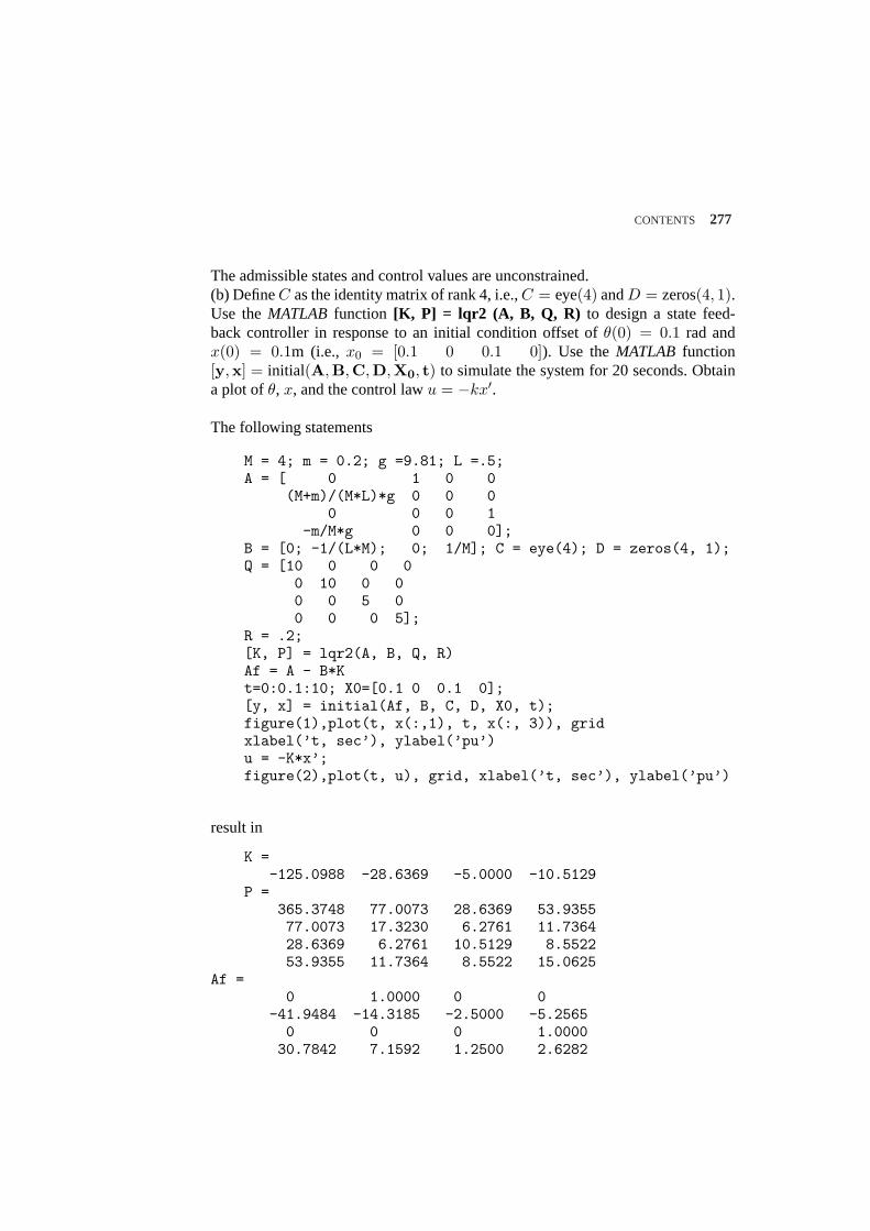
CONTENTS 277
The admissible states and control values are unconstrained.(b) DefineC as the identity matrix of rank 4, i.e.,C = eye(4) andD = zeros(4, 1).Use theMATLAB function [K, P] = lqr2 (A, B, Q, R) to design a state feed-back controller in response to an initial condition offset ofθ(0) = 0.1 rad andx(0) = 0.1m (i.e., x0 = [0.1 0 0.1 0]). Use theMATLAB function[y,x] = initial(A,B,C,D,X0, t) to simulate the system for 20 seconds. Obtaina plot ofθ, x, and the control lawu = −kx′.
The following statements
M = 4; m = 0.2; g =9.81; L =.5;A = [ 0 1 0 0
(M+m)/(M*L)*g 0 0 00 0 0 1
-m/M*g 0 0 0];B = [0; -1/(L*M); 0; 1/M]; C = eye(4); D = zeros(4, 1);Q = [10 0 0 0
0 10 0 00 0 5 00 0 0 5];
R = .2;[K, P] = lqr2(A, B, Q, R)Af = A - B*Kt=0:0.1:10; X0=[0.1 0 0.1 0];[y, x] = initial(Af, B, C, D, X0, t);figure(1),plot(t, x(:,1), t, x(:, 3)), gridxlabel(’t, sec’), ylabel(’pu’)u = -K*x’;figure(2),plot(t, u), grid, xlabel(’t, sec’), ylabel(’pu’)
result in
K =-125.0988 -28.6369 -5.0000 -10.5129
P =365.3748 77.0073 28.6369 53.935577.0073 17.3230 6.2761 11.736428.6369 6.2761 10.5129 8.552253.9355 11.7364 8.5522 15.0625
Af =0 1.0000 0 0
-41.9484 -14.3185 -2.5000 -5.25650 0 0 1.000030.7842 7.1592 1.2500 2.6282
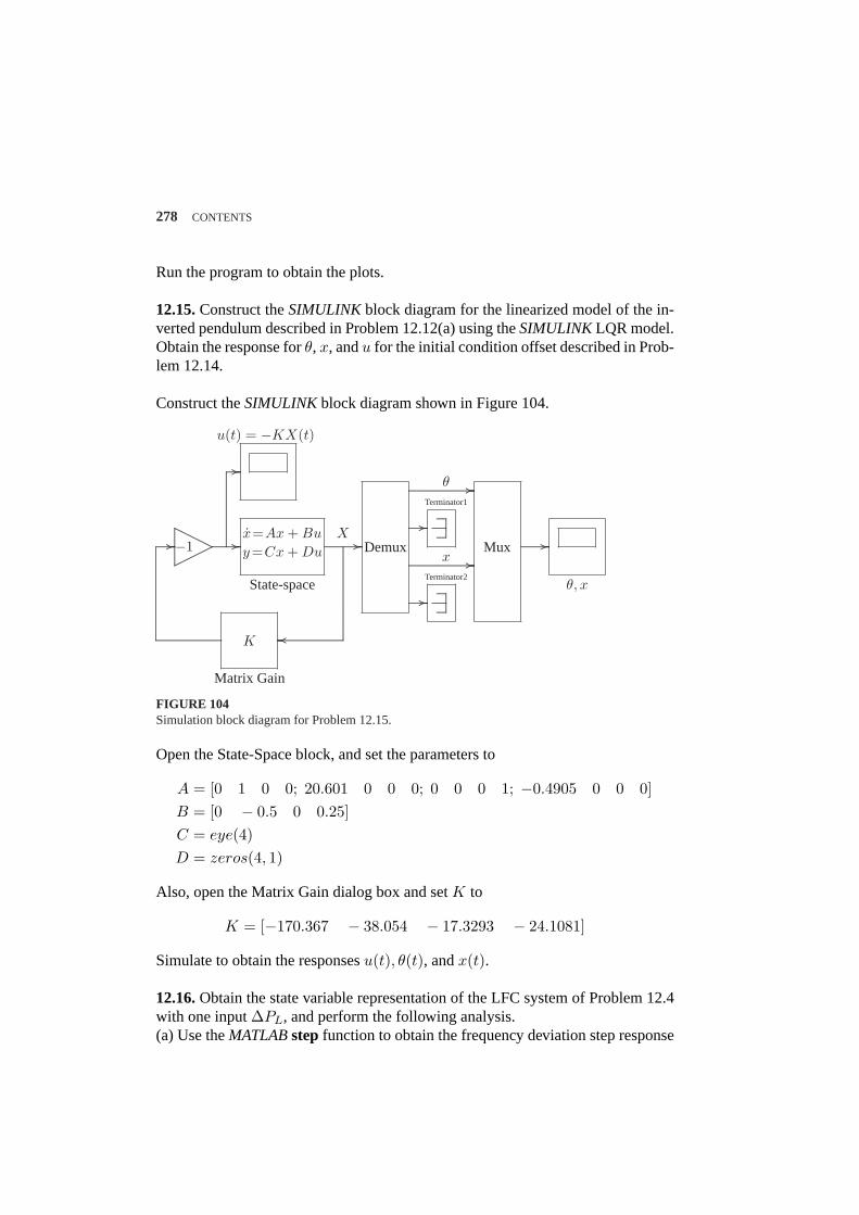
278 CONTENTS
Run the program to obtain the plots.
12.15.Construct theSIMULINK block diagram for the linearized model of the in-verted pendulum described in Problem 12.12(a) using theSIMULINKLQR model.Obtain the response forθ, x, andu for the initial condition offset described in Prob-lem 12.14.
Construct theSIMULINKblock diagram shown in Figure 104.
...................................................................................................................................................................................................................................................................................................................................... ................ −1 ........
........
........
........
........
........
........
........
........
........
........
........
........
........
........
........
............................................ ................
u(t) = −KX(t)
........
........
........
........
........
........
........
........
....................................................................................................................................................
................................................................. ................x=Ax + Bu
y=Cx + Du
State-space
.................................................................................. ................X
Demux
.................................................................................................................................. ................
.................................................................................................................................. ................
Mux ................................................................. ................
θ, x
.....................................................................................................................................................................................................................................................................................................................K
Matrix Gain
θ
x
................................................. ...................................................................................
.........................
Terminator1
................................................. ...................................................................................
.........................
Terminator2
FIGURE 104Simulation block diagram for Problem 12.15.
Open the State-Space block, and set the parameters to
A = [0 1 0 0; 20.601 0 0 0; 0 0 0 1; −0.4905 0 0 0]B = [0 − 0.5 0 0.25]C = eye(4)D = zeros(4, 1)
Also, open the Matrix Gain dialog box and setK to
K = [−170.367 − 38.054 − 17.3293 − 24.1081]
Simulate to obtain the responsesu(t), θ(t), andx(t).
12.16.Obtain the state variable representation of the LFC system of Problem 12.4with one input∆PL, and perform the following analysis.(a) Use theMATLABstepfunction to obtain the frequency deviation step response

CONTENTS 279
for a sudden load change of∆PL = 0.2 per unit.(b) Construct theSIMULINKblock diagram and obtain the frequency deviation re-sponse for the condition in part (a).(c) Useplacepol(A, B, C, p)function to place the compensated closed-loop pole at−4± j6 and -4. Obtain the frequency deviation step response of the compensatedsystem.(d) Construct theSIMULINKblock diagram and obtain the frequency deviation re-sponse for the condition in part (c).
From (12.54), the state equation of the LFC system of Problem 12.4 is
˙∆PV˙∆Pm
∆ω
=
−4 0 −1002 −2 00 0.0625 −0.1
∆PV
∆Pm
∆ω
+
00
−0.0625
∆PL
and the output equation is
y(t) = [0 0 1]
x1
x2
x3
For part (a) and (c), we use the following statements
PL = 0.2;A = [-4 0 -100; 2 -2 0; 0 0.0625 -0.1];B = [0; 0; -0.0625]; BPL = B*PL;C = [0 0 1]; D = 0;disp(’(a)’)t=0:0.02:10;[y, x] = step(A, BPL, C, D, 1, t);figure(1), plot(t, y), gridxlabel(’t, sec’), ylabel(’pu’)r =eig(A)disp(’(c) Pole-placement design’)P=[-4+j*6 -4-j*6 -4];[K, Af] = placepol(A, B, C, P);t=0:0.02:4;[y, x] = step(Af, BPL, C, D, 1, t);figure(2), plot(t, y), gridxlabel(’t, sec’), ylabel(’pu’)
The result is
(a)
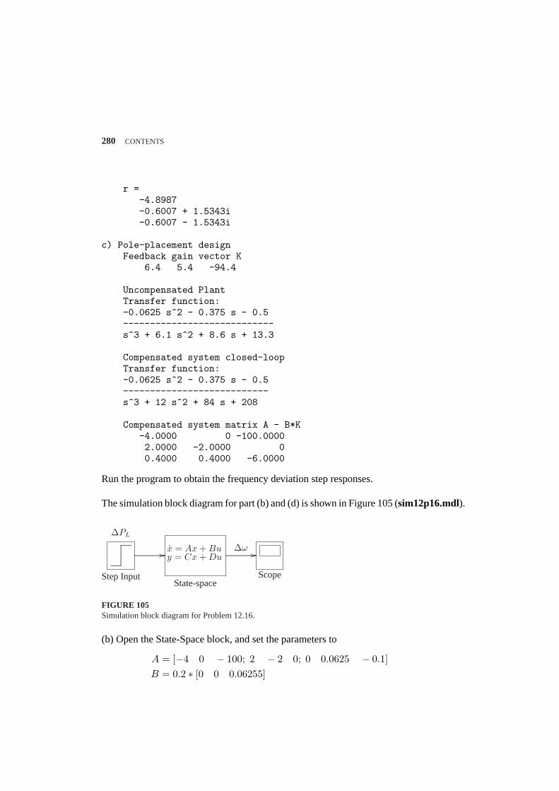
280 CONTENTS
r =-4.8987-0.6007 + 1.5343i-0.6007 - 1.5343i
c) Pole-placement designFeedback gain vector K
6.4 5.4 -94.4
Uncompensated PlantTransfer function:-0.0625 s^2 - 0.375 s - 0.5----------------------------s^3 + 6.1 s^2 + 8.6 s + 13.3
Compensated system closed-loopTransfer function:-0.0625 s^2 - 0.375 s - 0.5---------------------------s^3 + 12 s^2 + 84 s + 208
Compensated system matrix A - B*K-4.0000 0 -100.00002.0000 -2.0000 00.4000 0.4000 -6.0000
Run the program to obtain the frequency deviation step responses.
The simulation block diagram for part (b) and (d) is shown in Figure 105 (sim12p16.mdl).
...............................................................................................................
Step Input
∆PL
.................................................................................................. ................x = Ax + Buy = Cx + Du
State-space
.................................................................................................. ................∆ω
Scope
FIGURE 105Simulation block diagram for Problem 12.16.
(b) Open the State-Space block, and set the parameters to
A = [−4 0 − 100; 2 − 2 0; 0 0.0625 − 0.1]B = 0.2 ∗ [0 0 0.06255]
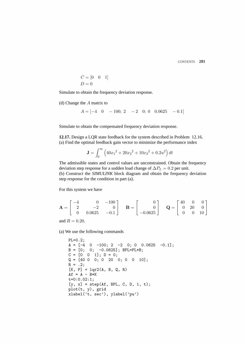
CONTENTS 281
C = [0 0 1]D = 0
Simulate to obtain the frequency deviation response.
(d) Change theA matrix to
A = [−4 0 − 100; 2 − 2 0; 0 0.0625 − 0.1]
Simulate to obtain the compensated frequency deviation response.
12.17.Design a LQR state feedback for the system described in Problem 12.16.(a) Find the optimal feedback gain vector to minimize the performance index
J =∫ ∞
0
(40x1
2 + 20x22 + 10x3
2 + 0.2u2)
dt
The admissible states and control values are unconstrained. Obtain the frequencydeviation step response for a sudden load change of∆PL = 0.2 per unit.(b) Construct theSIMULINK block diagram and obtain the frequency deviationstep response for the condition in part (a).
For this system we have
A =
−4 0 −100
2 −2 00 0.0625 −0.1
B =
00
−0.0625
Q =
40 0 00 20 00 0 10
andR = 0.20.
(a) We use the following commands
PL=0.2;A = [-4 0 -100; 2 -2 0; 0 0.0625 -0.1];B = [0; 0; -0.0625]; BPL=PL*B;C = [0 0 1]; D = 0;Q = [40 0 0; 0 20 0; 0 0 10];R = .2;[K, P] = lqr2(A, B, Q, R)Af = A - B*Kt=0:0.02:1;[y, x] = step(Af, BPL, C, D, 1, t);plot(t, y), gridxlabel(’t, sec’), ylabel(’pu’)
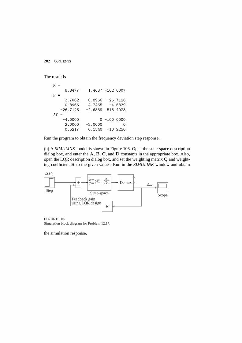
282 CONTENTS
The result is
K =8.3477 1.4637 -162.0007
P =3.7062 0.8966 -26.71260.8966 4.7465 -4.6839
-26.7126 -4.6839 518.4023Af =
-4.0000 0 -100.00002.0000 -2.0000 00.5217 0.1540 -10.2250
Run the program to obtain the frequency deviation step response.
(b) A SIMULINK model is shown in Figure 106. Open the state-space descriptiondialog box, and enter theA, B, C, andD constants in the appropriate box. Also,open the LQR description dialog box, and set the weighting matrixQ and weight-ing coefficientR to the given values. Run in theSIMULINK window and obtain
...................................................................................................
Step
∆PL
................................................................................................................................................... ................ +−......................................................... ................
x=Ax+Buy=Cx+Du
State-space
......................................................... ................ Demux
....................
....................
................................................................................................................................................................... ................
...................................................................................................................................................................................................................
................................................. ................ ∆ω
K
Feedback gainusing LQR design
Scope
FIGURE 106Simulation block diagram for Problem 12.17.
the simulation response.