Copyright © A. A. Frempong Solutions of the Navier-Stokes Equations -Abstract

1

Solutions of Navier-Stokes Equationsplus

Solutions of Magnetohydrodynamic Equations

AbstractAfter nearly 150 years of patience, the Navier-Stokes equations in 3-D for incompressible fluid flowhave been analytically solved by two different methods. In fact, it is shown that these equationscan be solved in 4-dimensions or n-dimensions. The author has proposed and applied a new law, the law of definite ratio for fluid flow. This law states that in incompressible fluid flow, theother terms of the fluid flow equation divide the gravity term in a definite ratio, and each termutilizes gravity to function. The sum of the terms of the ratio is always unity. This law evolvedfrom the author's earlier solutions of the Navier-Stokes equations. By applying the above law, thehitherto unsolved magnetohydrodynamic equations were routinely solved. It is also shown thatwithout gravity forces on earth, there will be no incompressible fluid flow on earth as is known.In addition to the usual method of solving these equations, the N-S equations have also beensolved by a second method in which the three equations in the system are added to produce asingle equation which is then integrated. The solutions by the two methods are identical, exceptfor the constants involved. Ratios were used to split the equations; and the resulting sub-equations were readily integrable, and even, the nonlinear sub-equations were readily integrated.The preliminaries reveal how the ratio technique evolved as well as possible applications of thesolution method in mathematics, science, engineering, business, economics, finance, investmentand personnel management decisions. The x−direction Navier-Stokes equation will be linearized,solved, and the solution analyzed. The linearized equation represents, except for the numericalcoefficient of the acceleration term, the linear part of the Navier-Stokes equation. This solutionwill be followed by the solution of the Euler equation of fluid flow. The Euler equationrepresents the nonlinear part of the Navier-Stokes equation. The Euler equation was solved in theauthor's previous paper. Following the Euler solution, the Navier-Stokes equation will be solved,essentially by combining the solutions of the linearized equation and the Euler solution. For theNavier-Stokes equation, the linear part of the relation obtained from the integration of the linearpart of the equation satisfied the linear part of the equation; and the relation from the integrationof the non-linear part satisfied the non-linear part of the equation. For the linearized equation,different terms of the equation were made subjects of the equation, and each such equation wasintegrated by first splitting-up the equation, using ratio, into sub-equations. The integrationresults were combined. Six equations were integrated. The relations obtained using these termsas subjects of the equations were checked in the corresponding equations. Only the equation withthe gravity term as subject of the equation satisfied its corresponding equation, and this uniquesolution led to the law of definite ratio for fluid flow, stated above. This equation which satisfiedits corresponding equation will be defined as the driver equation; and each of the other equationswhich did not satisfy its corresponding equation will be called a supporter equation. A supporterequation does not satisfy its corresponding equation completely but provides useful informationwhich is not apparent in the solution of the driver equation. The solutions and relations revealedthe role of each term of the Navier-Stokes equations in fluid flow. The gravity term is theindispensable term in fluid flow, and it is involved in the parabolic and forward motion of fluids.The pressure gradient term is also involved in the parabolic motion. The viscosity terms areinvolved in the parabolic, periodic and decreasingly exponential motion. Periodicity increaseswith viscosity. The variable acceleration term is also involved in the periodic and decreasinglyexponential motion. The convective acceleration terms produce square root function behaviorand fractional terms containing square root functions with variables in the denominators andconsequent turbulence behavior. For a spin-off, the smooth solutions from above are specializedand extended to satisfy the requirements of the CMI Millennium Prize Problems, and thus provethe existence of smooth solutions of the Navier-Stokes equations.

Solutions of the Navier-Stokes Equations

2

Options Option 1: Solutions of 3-D Linearized Navier-Stokes Equations (Method 1) 3 Option 2: Solutions of 4-D Linearized Navier-Stokes Equations 17 Option 3: Solutions of the Euler Equations 18 Option 4: Solutions of 3-D Navier-Stokes Equations (Method 1) 20 Option 5: Solutions of 4-D Navier-Stokes Equations 22 Option 5b: Two-term Linearized Navier-Stokes Equation (one nonlinear term) 22 Option 6: Solutions of Magnetohydrodynamic Equations 26 Option 7: Solutions of 3-D Navier-Stokes Equations (Method 2) 34 Option 8: Solutions of 3-D Linearized Navier-Stokes Equation (Method 2) 40 Option 9: CMI Millennium Prize Problem Requirements 44

The Navier-Stokes equations in three dimensions are three simultaneous equations in Cartesiancoordinates for the flow of incompressible fluids. The equations are presented below:

(N

μ ∂∂

∂∂

∂∂

∂∂ ρ ρ ∂

∂∂∂

∂∂

∂∂

μ∂∂

∂∂

∂∂

∂∂ ρ ρ

∂∂

( ) ( )

( ) (

)2

2

2

2

2

2

2

2

2

2

2

2

Vx

Vy

Vz

px

gVt

VVx

VVy

VVz

Vx

Vy

Vz

py

gVt

x x x xx

xy

xz

xx x

y y yy

y

+ + − + = + + +

+ + − + = + VVVx

VVy

VVz

Vx

Vy

Vz

pz

gVt

VVx

VVy

VVz

x z

z z z zx

zy

zz

z

yy

y y

z

y

z

∂∂

∂∂

∂∂

μ ∂∂

∂∂

∂∂

∂∂ ρ ρ ∂

∂∂∂

∂∂

∂∂

+ +

+ + − + = + + +

⎧

⎨

⎪⎪⎪

⎩

⎪⎪⎪

)

( ) ( )

)

)

(N

(N

2

2

2

2

2

2

Equation ( Nx ) will be the first equation to be solved; and based on its solution, one will be able towrite down the solutions for the other two equations, ( Ny), and ( Nz ).

Dimensional ConsistencyThe Navier-Stokes equations are dimensionally consistent as shown below:

μ∂∂

∂∂

∂∂

∂∂ ρ ρ ∂

∂∂∂

∂∂

∂∂( ) ( )

2

2

2

2

2

2

V

x

V

yVz

px

gVt

VVx

VVy

VVz

x x x xx

xx

xy

xz

x + + − + = + + +

Using MLT

M L T L T L T L T L T M L T L T L T L T( ) ( )− − − − − − − − − − − − − − − − − −+ + − + = + + +2 2 2 2 2 2 2 2 2 2 2 2 2 2 2 2 2 2

Using kg m s− −kg m s m s m s m s m s kg m s m s m s m s( (− − − − − − − − − − − − − − − − − −+ + − + = + + +2 2 2 2 2 2 2 2 2 2 2 2 2 2 2 2 2 2

Option 1

Option 9Option 8

Option 5bOption 5

Option 6

Option 4Option 3Option 2

Option 7

Solutions of the Navier-Stokes EquationsPreliminaries

3

Option 1Solution of 3-D Linearized Navier-Stokes Equation

in the x-directionThe equation will be linearized by redefinition. The nine-term equation will be reduced to six terms.

Given: μ ∂∂

∂∂

∂∂

∂∂ ρ ρ ∂

∂∂∂

∂∂

∂∂( ) ( )

2

2

2

2

2

2Vx Vx Vx x Vx

xVx

yVx

zVx

x y zpx

gx tV

xV

yV

z+ + − + = + + + (A)

− − − + + + + + =μ ∂∂ μ ∂

∂ μ ∂∂

∂∂ ρ ∂

∂ ρ ∂∂ ρ ∂

∂ ρ ∂∂ ρ

2

2

2

2

2

2Vx Vx Vx x Vx

xVx

yVx

zVx

x y zpx t

Vx

Vy

Vz

gx (B)

− + + + + =μ ∂∂

∂∂

∂∂

∂∂ ρ ∂

∂ ρ( ) ( )2

2

2

2

2

2 4Vx Vx Vx x Vx

x y zpx t

gx (C)

Plan: One will split-up equation (C) into five equations, solve them, and combine the solutions. Onsplitting-up the equations and proceeding to solve them, the non linear terms could be redefined andmade linear. This linearization is possible if the gravitational force term is the subject of theequation as in equation (B). After converting the non-linear terms to linear terms by redefinition,one will have only six terms as in equation (C). One will show logically how equation (C) wasobtained from equation (B), using a method which will be called the multiplier method.Three main steps are covered.In main Step 1, one shows how equation (C) was obtained from equation (B)In main Step 2, equation (C) will be split-up into five equations.In main Step 3, each equation will be solved.In main Step 4, the solutions from the five equations will be combined.In main Step 5, the combined relation will be checked in equation (C). for identity.

PreliminariesHere, one covers examples to illustrate the mathematical validity of how one splits-up equation (C).Let one think like a child - Albert Einstein. Actually, one can think like an eighth or a ninth grader. Suppose one performs the following operations:

Example 1: 10 20 25 55+ + = (1) 10 55 5510

55211= =× × (2)

20 55 552055

411= =× × (3)

25 55 552555

511= =× × (4)

Equations (2), (3), and (4) can be written as follows:

10 55= a (5) 20 55= b (6) 25 55= c (7) One will call a b, and c multipliers.

Above, a = 211, b = 4

11 , c = 511

Observe also that a b c+ + = 1( 2

114

115

111111 1+ + = = )

Back to Options

Solutions of the Navier-Stokes EquationsPreliminaries

4

Example 2: Addition of only two numbers 20 25 45+ = (8) 20 45 4520

4549= =× × (9)

25 45 452545

59= =× × (10)

Equations (9), and (10), can be written as follows: 20 45= a (11) 25 45= b (12) Rewrite (8) by transposition. If 20 45 25− = − Then 20 25= − d ( d is a multiplier) − = −45 25 f ( f is a multiplier)

Above, d = − = −2025

45 , f = −

− =4525

95 ,

Observe also here that d f+ = 1 ( − + = =45

95

55 1)

a b+ = 1 ( 49

59

99 1+ = = )

One can conclude that the sum of the multipliers is always 1.

More formally: Let A B C S+ + = , where A B C S, , and . are real numbers. (for the moment), and one excludes 0. Let a b c, , be respectively, multipliers of the sum S corresponding to A B C, , . Then A Sa= , B Sb= , C Sc= ; and a b c+ + = 1 To show that a b c+ + = 1, Sa Sb Sc S+ + = . S a b c S( )+ + = (factoring out the S) a b c+ + = 1. (Dividing both sides of the equation by S)

Solutions of the Navier-Stokes EquationsPreliminaries

5

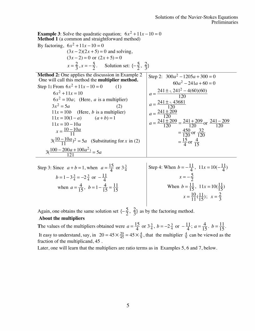
Example 3: Solve the quadratic equation; 6 11 10 02x x+ − =Method 1 (a common and straightforward method)By factoring, 6 11 10 02x x+ − = ( )( )3 2 2 5 0x x− + = and solving, ( )3 2 0x − = or ( )2 5 0x + = x = 2

3 , x = − 52 . Solution set: { , }− 5

223

Method 2: One applies the discussion in Example 2 One will call this method the multiplier method.Step 1: From 6 11 10 02x x+ − = (1) 6 11 102x x+ = 6 102x a= ; (Here, a is a multiplier) 3 52x a= (2) 11 10x b= (Here, b is a multiplier) 11 10 1x a= −( ) ( )a b+ = 1 11 10 10x a= − x a= −10 10

11 3 10 10

11 52( )− =a a (Substituting for x in (2)

3 100 200 100121 5

2( )− + =a a a

Step 2: 300 1205 300 02a a− + = 60 241 60 02a a− + =

a

a

a

a

= ± −

= ±

= ±

= ± = + −

=

=

241 241 4 60 60120

241 43681120

241 209120

241 209120

241 209120

241 209120

450120

32120

154

415

2 ( )( )

or

or

or

Step 3: Since a b+ = 1, when a = 154 3 3

4 or

b = − = − −1 3 2 114

34

34 or

when a b= = − =415 1 4

151115,

Step 4: When b = − 114 , 11 10 11

4x = −( )

x = − 52

When b = 1115 , 11 10 11

15x = ( )

x = 1011

1115( ); x = 2

3

Again, one obtains the same solution set { , }− 52

23 as by the factoring method.

About the multipliers

The values of the multipliers obtained were a = 154 3 3

4 or , b = − −2 114

34 or ; a b= =4

151115. .

It easy to understand, say, in 20 45 452045

49= =× × , that the multiplier 4

9 can be viewed as thefraction of the multiplicand, 45 .Later, one will learn that the multipliers are ratio terms as in Examples 5, 6 and 7, below.

Solutions of the Navier-Stokes EquationsPreliminaries

6

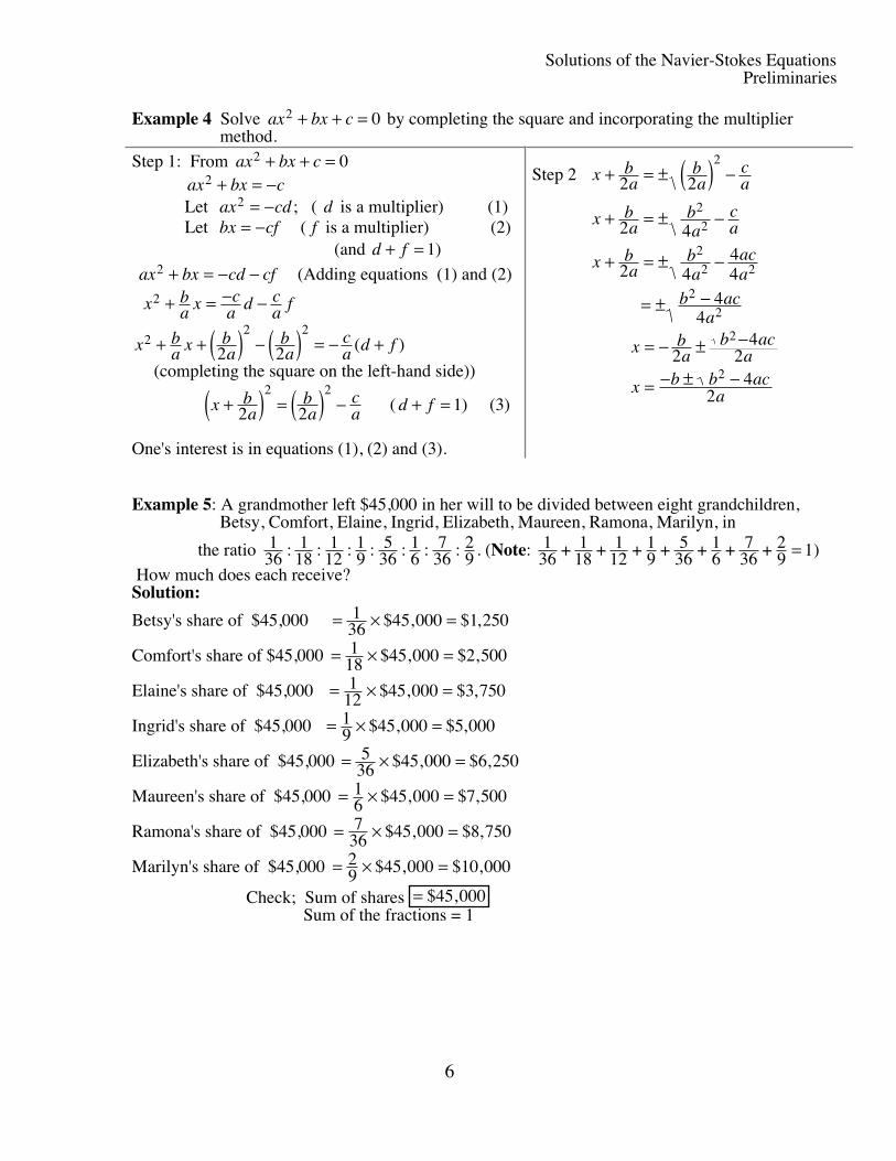
Example 4 Solve ax bx c2 0+ + = by completing the square and incorporating the multiplier method.

Step 1: From ax bx c2 0+ + = ax bx c2 + = − Let ax cd2 = − ; ( d is a multiplier) (1) Let bx cf= − ( f is a multiplier) (2) (and d f+ = 1)

ax bx cd cf2 + = − − (Adding equations (1) and (2)

x ba x c

a d ca f2 + = − −

x ba x b

aba

ca d f2

2 2

2 2+ + ( ) − ( ) = − +( )

(completing the square on the left-hand side))

x ba

ba

ca+( ) = ( ) −2 2

2 2 ( d f+ = 1) (3)

One's interest is in equations (1), (2) and (3).

Step 2 x ba

ba

ca+ = ± ( ) −2 2

2

x ba

ba

ca

x ba

ba

aca

b aca

x ba

b aca

x b b aca

+ = ± −

+ = ± −

= ± −

= − ± −

= − ± −

2 4

2 444

44

24

24

2

2

2

2

2 2

2

2

2

2

Example 5: A grandmother left $45,000 in her will to be divided between eight grandchildren, Betsy, Comfort, Elaine, Ingrid, Elizabeth, Maureen, Ramona, Marilyn, in

the ratio 136 : 1

18 : 112 : 1

9 : 536 : 1

6 : 736 : 2

9 . (Note: 136 + 1

18 + 112 + 1

9 + 536 + 1

6 + 736 + 2

9 = 1)

How much does each receive?Solution:

Betsy's share of $45,000 = × =1 $45,000 $36 1 250,

Comfort's share of $45,000 = × =1 $45,000 $18 2 500,

Elaine's share of $45,000 = × =1 $45,000 $ 75012 3,

Ingrid's share of $45,000 = × =1 $45,000 $9 5 000,

Elizabeth's share of $45,000 = × =5 $45,000 $36 6 250,

Maureen's share of $45,000 = × =1 $45,000 $6 7 500,

Ramona's share of $45,000 = × =7 $45,000 $ ,75036 8

Marilyn's share of $45,000 = × =2 $45,000 $9 10 000,

Check; Sum of shares = $45,000 Sum of the fractions = 1

Solutions of the Navier-Stokes EquationsPreliminaries

7

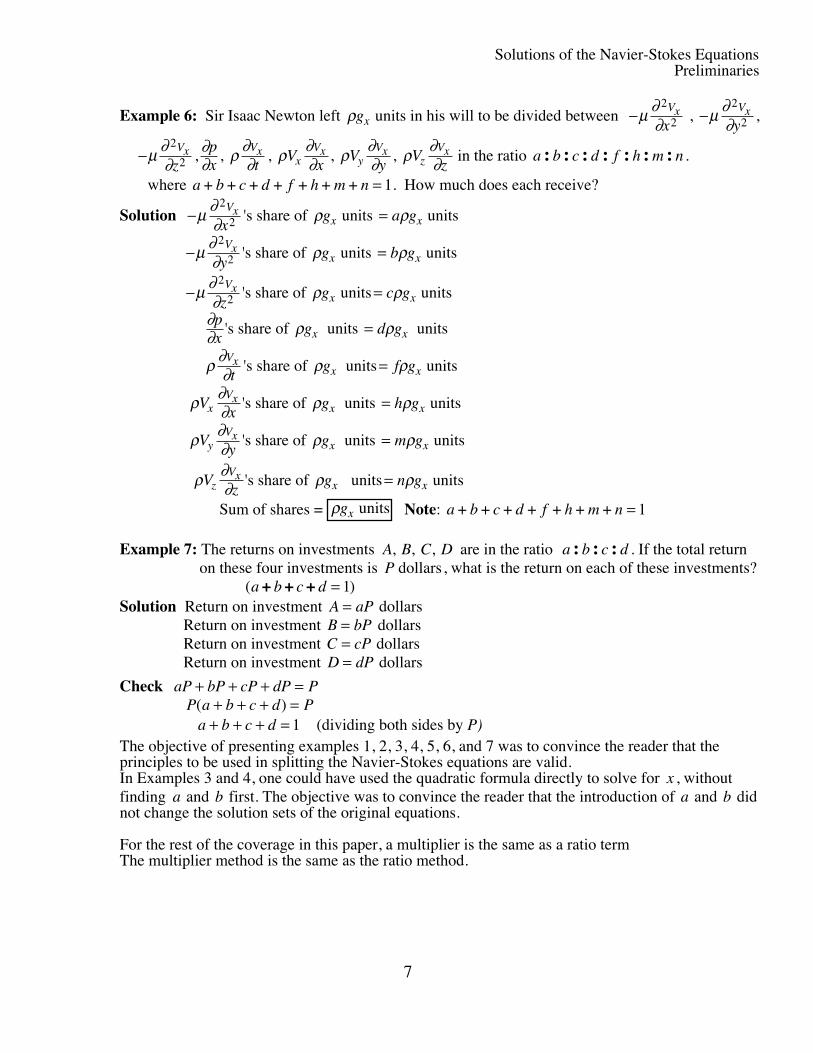
Example 6: Sir Isaac Newton left ρgx units in his will to be divided between −μ ∂∂

2

2Vx

x , −μ ∂

∂2

2Vx

y,

−μ ∂∂2

2Vx

z,∂∂px

, ρ ∂∂Vxt

, ρ ∂∂Vxx

Vx , ρ ∂∂Vyy

Vx , ρ ∂∂Vzz

Vx in the ratio a b c d f h m n: : : : : : : .

where a b c d f h m n+ + + + + + + = 1. How much does each receive?

Solution −μ ∂∂

2

2Vx

x's share of ρgx units = a gxρ units

−μ ∂∂

2

2Vx

y's share of ρgx units = b gxρ units

−μ ∂∂2

2Vx

z's share of ρgx units = c gxρ units

∂∂px

's share of ρgx units = d gxρ units

ρ ∂∂Vxt

's share of ρgx units = f gxρ units

ρ ∂∂Vxx

Vx 's share of ρgx units = h gxρ units

ρ ∂∂Vyy

Vx 's share of ρgx units = m gxρ units

ρ ∂∂Vzz

Vx 's share of ρgx units = n gxρ units

Sum of shares = ρgx units Note: a b c d f h m n+ + + + + + + = 1

Example 7: The returns on investments A B C D, , , are in the ratio a b c d: : : . If the total return on these four investments is P dollars, what is the return on each of these investments? ( )a b c d+ + + = 1Solution Return on investment A aP= dollars Return on investment B bP= dollars Return on investment C cP= dollars Return on investment D dP= dollars

Check aP bP cP dP P+ + + = P a b c d P( )+ + + = a b c d+ + + = 1 (dividing both sides by P)The objective of presenting examples 1, 2, 3, 4, 5, 6, and 7 was to convince the reader that theprinciples to be used in splitting the Navier-Stokes equations are valid.In Examples 3 and 4, one could have used the quadratic formula directly to solve for x , withoutfinding a and b first. The objective was to convince the reader that the introduction of a and b didnot change the solution sets of the original equations.

For the rest of the coverage in this paper, a multiplier is the same as a ratio termThe multiplier method is the same as the ratio method.

Linearization of Non-Linear terms

8

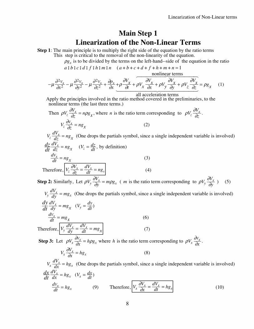
Main Step 1Linearization of the Non-Linear Terms

Step 1: The main principle is to multiply the right side of the equation by the ratio terms This step is critical to the removal of the non-linearity of the equation. ρgx is to be divided by the terms on the left-hand--side of the equation in the ratio a b c d f h m n: : : : : : : ( a b c d f h m n+ + + + + + + = 1

− − − + + + + + =μ ∂∂ μ ∂

∂ μ ∂∂

∂∂ ρ

∂∂ ρ

∂∂ ρ

∂∂ ρ

∂∂ ρ

2

2

2

2

2

2Vx Vx Vx x

x y zpx

Vxt

VxVxx

VyVxy

VzVxz

gx

nonlinear terms

all acceleration terms

6 744444 844444

1 24444444 34444444 (1)

Apply the principles involved in the ratio method covered in the preliminaries, to the nonlinear terms (the last three terms.)

Then ρ ∂∂ ρVVz

n gxzx = , where n is the ratio term corresponding to ρ ∂

∂VVzzx .

Vz

ngxzVx∂

∂ = (2)

VdVdz ngxz

x = (One drops the partials symbol, since a single independent variable is involved)

dzdt

dVdz ngx V dz

dtx

z= = ( , by definition)

ddt ngxVx = (3)

Therefore, VVz

dVdt ngz

x xx

∂∂ = = (4)

Step 2: Similarly, Let ρ ∂∂ ρVVy

m gyx

x= ( m is the ratio term corresponding to ρ ∂∂VVyyx ) (5)

VdVdy mgy

xx= (One drops the partials symbol, since a single independent variable is involved)

dydt

dVdy mgx V

dydt

xy= = ( )

ddt mgxVx = (6)

Therefore, VdVdy

dVdt mgxy

x x= = (7)

Step 3: Let ρ ∂∂ ρVx

h gxVx

x= where h is the ratio term corresponding to ρ ∂∂Vxx

Vx .

VVx

hgxx

x∂∂ = (8)

VdVdx hgx

xx= (One drops the partials symbol, since a single independent variable is involved)

dxdt

dVdx hg V dx

dtx

x x= = ( )

ddt hgVx

x= (9) Therefore, VVx

dVdt hgx

x xx

∂∂ = = (10)

Linearization of Non-Linear terms

9

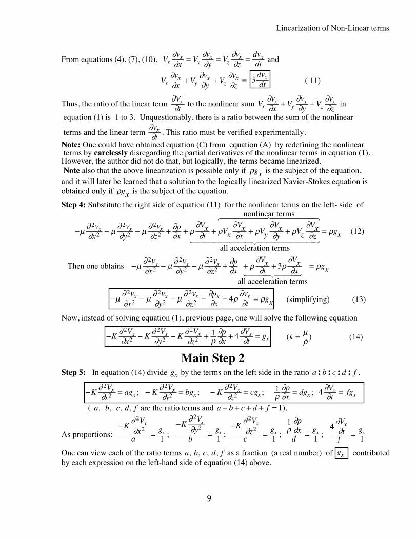
From equations (4), (7), (10), Vx

Vy

Vz

ddtx

Vxy

Vxz

Vx Vx∂∂

∂∂

∂∂= = = and

Vx

Vy

Vzx

Vxy

Vxz

Vx∂∂

∂∂

∂∂+ + = 3

ddtVx ( 11)

Thus, the ratio of the linear term ∂∂Vtx to the nonlinear sum V

xV

yV

zxVx

yVx

zVx∂

∂∂∂

∂∂+ + in

equation (1) is 1 to 3. Unquestionably, there is a ratio between the sum of the nonlinear

terms and the linear term ∂∂Vxt

. This ratio must be verified experimentally.

Note: One could have obtained equation (C) from equation (A) by redefining the nonlinear terms by carelessly disregarding the partial derivatives of the nonlinear terms in equation (1).However, the author did not do that, but logically, the terms became linearized. Note also that the above linearization is possible only if ρgx is the subject of the equation,and it will later be learned that a solution to the logically linearized Navier-Stokes equation isobtained only if ρgx is the subject of the equation.

Step 4: Substitute the right side of equation (11) for the nonlinear terms on the left- side of

− − − + + + + + =μ ∂∂ μ ∂

∂ μ ∂∂

∂∂ ρ

∂∂ ρ

∂∂ ρ

∂∂ ρ

∂∂ ρ

2

2

2

2

2

2Vx Vx Vx

x y zpx

Vxt

VxVxx

VyVxy

VzVxz

gx

nonlinear terms

all acceleration terms

6 744444 844444

1 24444444 34444444 (12)

Then one obtains − − − + + + =μ ∂∂ μ ∂

∂ μ ∂∂

∂∂ ρ

∂∂ ρ

∂∂ ρ

2

2

2

2

2

2 3Vx Vx Vx

x y zpx

Vxt

Vxx

gx

all acceleration terms1 2444 3444

− − − + + =μ ∂∂ μ ∂

∂ μ ∂∂

∂∂ ρ ∂

∂ ρ2

2

2

2

2

2 4Vx Vx Vx x Vx

x y zpx t

gx (simplifying) (13)

Now, instead of solving equation (1), previous page, one will solve the following equation

− − − + + =KVx

KVy

KVz

px

Vt

gx x x xx

∂∂

∂∂

∂∂ ρ

∂∂

∂∂

2

2

2

2

2

21 4 (k = μ

ρ ) (14)

Main Step 2Step 5: In equation (14) divide gx by the terms on the left side in the ratio a b c d f: : : : .

− = − = − = = =KV

ag KV

bg KV

cgpx

dgVt

fgxx x

xy x

xz x x x

x∂∂

∂∂

∂∂ ρ

∂∂

∂∂

2

2

2

2

2

21 4; ; ; ;

( a b c d f, , , , are the ratio terms and a b c d f+ + + + = 1).

As proportions: −

=−

=−

= = =K

Vx

ag

KV

yb

g KVz

cg

px

dg

Vt

fg

x x xx

x

x x x x

∂∂

∂∂

∂∂ ρ

∂∂

∂∂

2

2

2

2

2

2

1 1 1

1

1

4

1; ; ; ;

One can view each of the ratio terms a b c d f, , , , as a fraction (a real number) of gx contributedby each expression on the left-hand side of equation (14) above.

Solutions of the five sub-equations

10

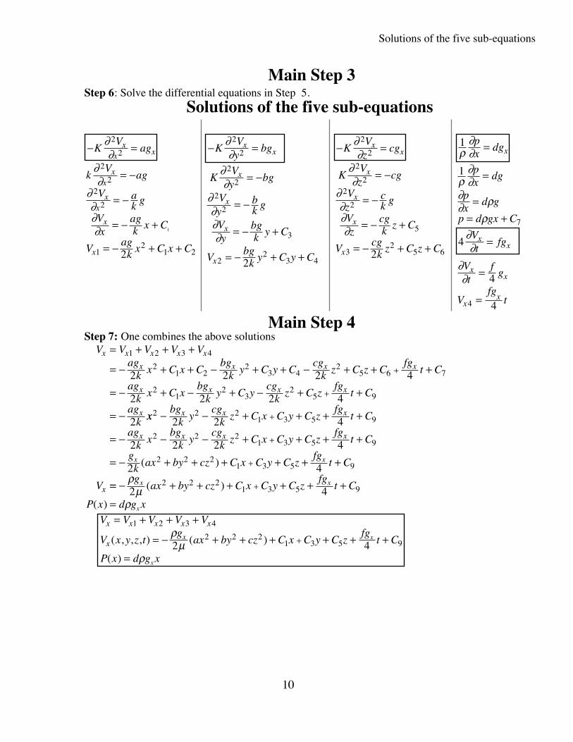
Main Step 3Step 6: Solve the differential equations in Step 5.

Solutions of the five sub-equations

− =KV

agxx x

∂∂2

2

kV

ag

V ak g

Vx

agk x C

Vag

k x C x C

xx

xx

x

x

∂∂

∂∂∂∂

2

22

2

12

1 2

1

2

= −

= −

= − +

= − + +

− =KVy

bgxx

∂∂2

2

KVy

bg

Vy

bk g

Vy

bgk y C

Vbg

k y C y C

x

x

x

x

∂∂

∂∂∂∂

2

2

2

2

3

22

3 42

= −

= −

= − +

= − + +

− =KVz

cgxx

∂∂2

2

KVz

cg

Vz

ck g

Vz

cgk z C

Vcgk z C z C

x

x

x

x

∂∂

∂∂∂∂

2

22

2

5

32

5 62

= −

= −

= − +

= − + +

1ρ

∂∂px

dgx=

1

7

ρ∂∂

∂∂ ρ

ρ

px

dg

px

d g

p d gx C

=

== +

4∂∂Vt

fgxx=

∂∂Vt

fgx

x= 4

Vfg

txx

4 4=

Main Step 4Step 7: One combines the above solutions

V V V V Vag

k x C x Cbg

k y C y Ccg

k z C z Cfg

t C

agk x C x

bgk y C y

cgk z C z

fgt C

agk

x x x x x

x x x x

x x x x

x

= + + +

= − + + − + + − + + +

= − + − + − + +

= −

+

+

1 2 3 4

21 2

23 4

25 6 7

21

23

25 9

2 2 2 4

2 2 2 4

2 xxbg

k ycg

k z C x C y C zfg

t C

agk x

bgk y

cgk z C x C y C z

fgt C

gk ax by cz C x C y C z

fgt C

V

x x x

x x x x

x

x x

2 2 21 3 5 9

2 2 21 3 5 9

2 2 21 3 5 9

2 2 4

2 2 2 4

2 4

− − + + + +

= − − − + + + +

= − + + + + + +

+

+

+( )

== − + + + + + +

=

+ρ

μρ

gax by cz C x C y C z

fgt C

P x d g x

x x

x

2 42 2 2

1 3 5 9( )

( )

V V V V V

V x y z tg

ax by cz C x C y C zfg

t C

P x d g x

x x x x x

xx x

x

= + + +

= − + + + + + +

=

+

1 2 3 4

2 2 21 3 5 92 4( , , , ) ( )

( )

ρμ

ρ

Checking in equation (C)

11

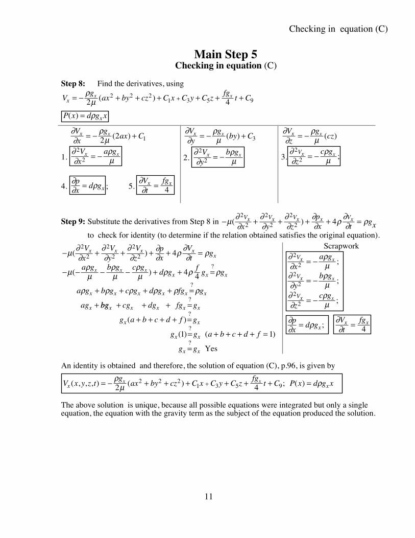
Main Step 5Checking in equation (C)

Step 8: Find the derivatives, using

Vg

ax by cz C x C y C zfg

t Cxx x= − + + + + + ++

ρμ2 4

2 2 21 3 5 9( )

P x d g xx( ) = ρ

∂∂

ρμ

Vx

gax Cx x= − +2 2 1( )

1. ∂∂

ρμ

2

2Vx

a gx x= −

4. ∂∂ ρpx

d gx= ; 5. ∂∂Vt

fgx x= 4

∂∂

ρμ

Vy

gby Cx x= − +( ) 3

2. ∂∂

ρμ

2

2Vy

b gx x= −

∂∂

ρμ

Vz

gczx x= − ( )

3.∂∂

ρμ

2

2Vx

zc gx= − ;

Step 9: Substitute the derivatives from Step 8 in − + + + + =μ ∂∂

∂∂

∂∂

∂∂ ρ ∂

∂ ρ( )2

2

2

2

2

2 4Vx Vx Vx x Vx

x y zpx t

gx to check for identity (to determine if the relation obtained satisfies the original equation).

− + + + + =

− − − − + + =

+ + + + =

+

μ ∂∂

∂∂

∂∂

∂∂ ρ ∂

∂ ρ

μ ρμ

ρμ

ρμ ρ ρ ρ

ρ ρ ρ ρ ρ ρ

( )

( )?

?

2

2

2

2

2

2 4

4 4

Vx

Vy

Vz

px

Vt

g

a g b g c gd g

fg g

a g b g c g d g fg g

ag

x x x xx

x x x

x x x x x x

x

x x x

bgbg cg dg fg g

g a b c d f g

g g a b c d f

g g

x x x x x

x x

x x

x x

(

Yes

+ + + =

+ + + + =

= + + + + =

=

?

?

?

?

( )

( ) )1 1

Scrapwork∂∂

ρμ

∂∂

ρμ

∂∂

ρμ

2

2

2

2

2

2

Vx

Vx

Vx

xa g

yb g

zc g

x

x

x

= −

= −

= −

;

;

;

∂∂ ρpx

d gx= ; ∂∂Vt

fgx x= 4

An identity is obtained and therefore, the solution of equation (C), p.96, is given by

V x y z tg

ax by cz C x C y C zfg

t C P x d g xx xx x( , , , ) ( ) ( )= − + + + + + + =+

ρμ ρ2 4

2 2 21 3 5 9;

The above solution is unique, because all possible equations were integrated but only a singleequation, the equation with the gravity term as the subject of the equation produced the solution.

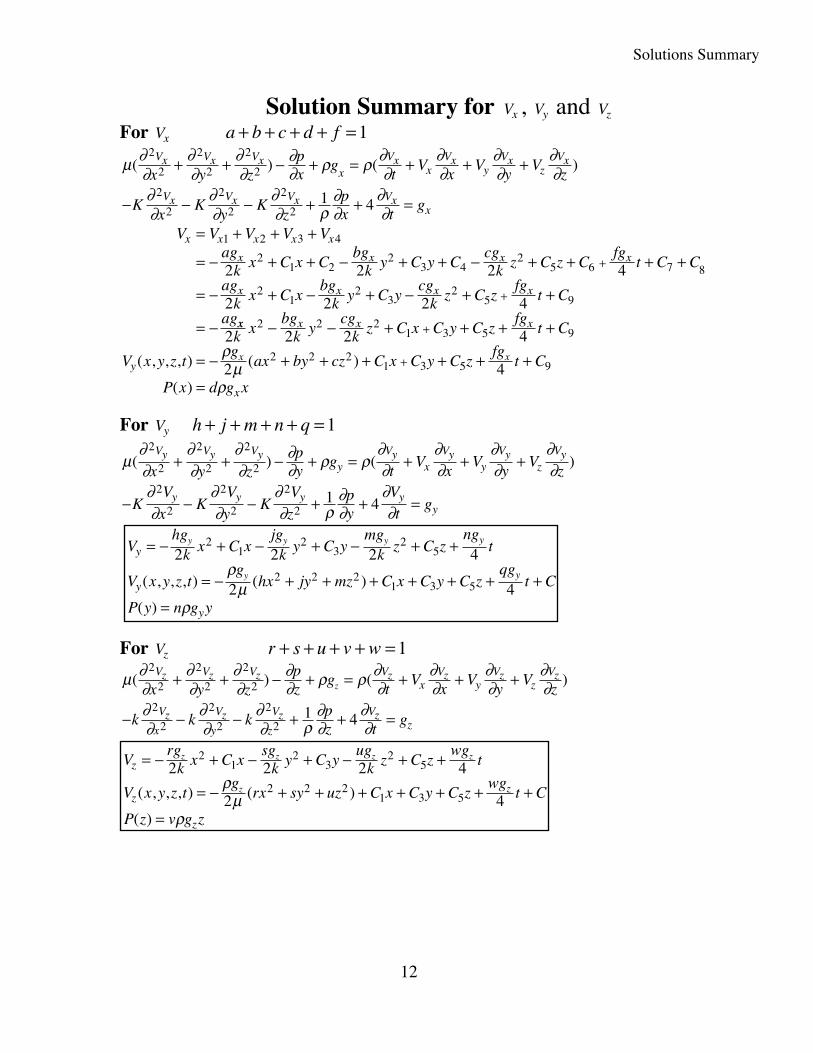
Solutions Summary

12

Solution Summary for Vx , Vy and Vz

For Vx a b c d f+ + + + = 1

μ ∂∂

∂∂

∂∂

∂∂ ρ ρ ∂

∂∂∂

∂∂

∂∂( ) ( )

2

2

2

2

2

2Vx Vx Vx

xVx

xVx

yVx

zVx

x y zpx

gt

Vx

Vy

Vz

+ + − + = + + +

− − − + + =Kx

Ky

Kz

px t

gVx Vx Vx Vx

x∂∂

∂∂

∂∂ ρ

∂∂

∂∂

2

2

2

2

2

21 4

V V V V Vag

k x C x Cbg

k y C y Ccg

k z C z Cfg

t C C

agk x C x

bgk y C y

cgk z C z

fgt C

ag

x x x x x

x x x x

x x x x

= + + +

= − + + − + + − + + + +

= − + − + − + +

= −

+

+

1 2 3 4

21 2

23 4

25 6 7 8

21

23

25 9

2 2 2 4

2 2 2 4xx x x x

y

x

k xbg

k ycg

k z C x C y C zfg

t C

V x y z tg

ax by cz C x C y C zfg

t C

P x d g x

x x

2 2 2 4

2 4

2 2 21 3 5 9

2 2 21 3 5 9

− − + + + +

= − + + + + + +

=

+

+( , , , ) ( )

( )

ρμ

ρ

For Vy h j m n q+ + + + = 1

μ∂∂

∂∂

∂∂

∂∂ ρ ρ

∂∂

∂∂

∂∂

∂∂( ) ( )

2

2

2

2

2

2

Vy Vy Vyy

Vyx

Vyy

Vyz

Vy

x y zpy

gt

Vx

Vy

Vz

+ + − + = + + +

− − − + + =KVx

KVy

KVz

py

Vt

gy y y yy

∂∂

∂∂

∂∂ ρ

∂∂

∂∂

2

2

2

2

2

21 4

Vhg

k x C xjg

k y C ymg

k z C zng

t

V x y z tg

hx jy mz C x C y C zqg

t C

P y n g y

y

y

y

y y y

y

y

y

= − + − + − + +

= − + + + + + + +

=

2 2 2 4

2 4

21

23

25

2 2 21 3 5( , , , ) ( )

( )

ρμ

ρ

For Vz r s u v w+ + + + = 1

μ ∂∂

∂∂

∂∂

∂∂ ρ ρ ∂

∂∂∂

∂∂

∂∂( ) ( )

2

2

2

2

2

2Vz Vz Vz Vz

xVz

yVz

zVz

x y zpz

gt

Vx

Vy

Vzz+ + − + = + + +

− − − + + =k k kpz t

gVz

x

Vzy

Vzz

Vzz

∂∂

∂∂

∂∂ ρ

∂∂

∂∂

2

2

2

2

2

21 4

Vrg

k x C xsg

k y C yug

k z C zwg

t

V x y z tg

rx sy uz C x C y C zwg

t C

P z v g z

z

z

z

z z z z

z z

= − + − + − + +

= − + + + + + + +

=

2 2 2 4

2 4

21

23

25

2 2 21 3 5( , , , ) ( )

( )

ρμ

ρ

Discussion About Solutions

13

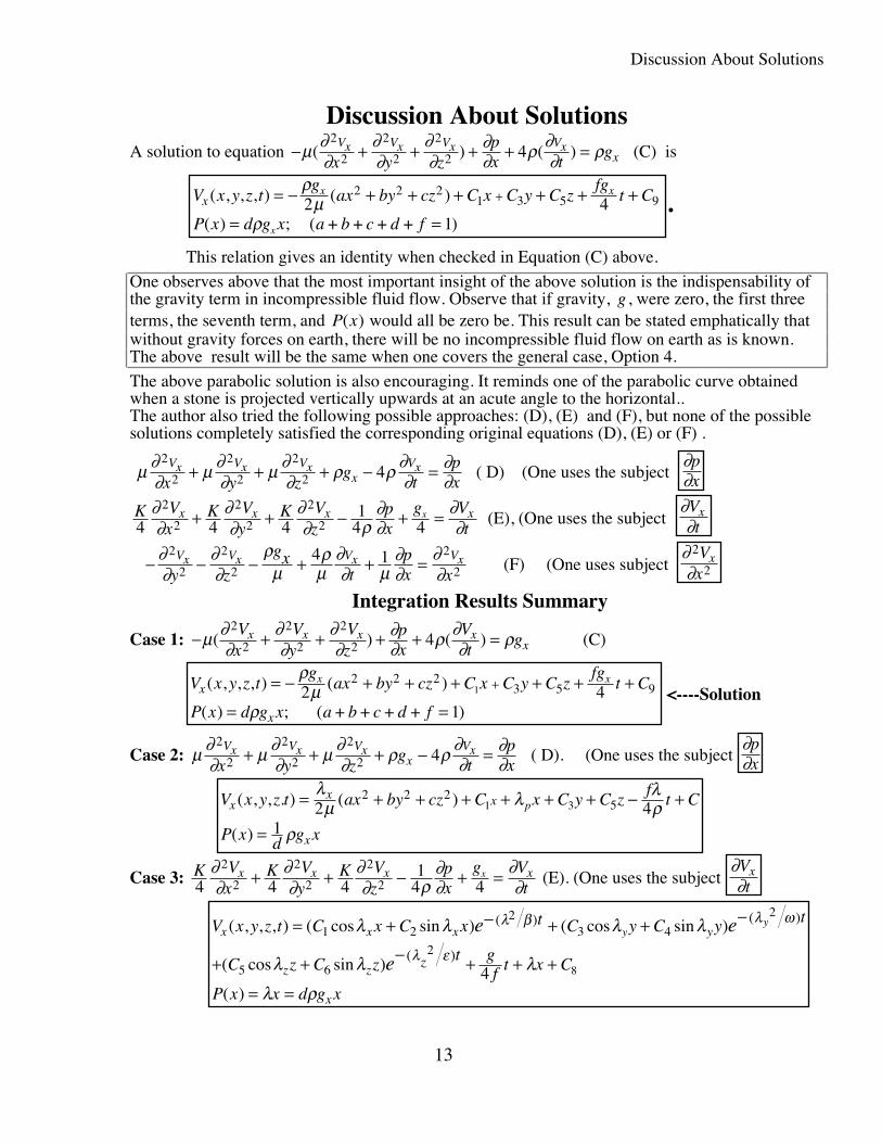
Discussion About SolutionsA solution to equation − + + + + =μ ∂

∂∂∂

∂∂

∂∂ ρ ∂

∂ ρ( ) ( )2

2

2

2

2

2 4Vx Vx Vx Vx

xx y zpx t

g (C) is

V x y z tg

ax by cz C x C y C zfg

t C

P x d g x a b c d f

xx x

x

( , , , ) ( )

( ) (

= − + + + + + +

= =

+ρ

μρ

2 41

2 2 21 3 5 9

; + + + + ).

This relation gives an identity when checked in Equation (C) above.

One observes above that the most important insight of the above solution is the indispensability ofthe gravity term in incompressible fluid flow. Observe that if gravity, g , were zero, the first threeterms, the seventh term, and P x( ) would all be zero be. This result can be stated emphatically thatwithout gravity forces on earth, there will be no incompressible fluid flow on earth as is known.The above result will be the same when one covers the general case, Option 4.

The above parabolic solution is also encouraging. It reminds one of the parabolic curve obtainedwhen a stone is projected vertically upwards at an acute angle to the horizontal..The author also tried the following possible approaches: (D), (E) and (F), but none of the possiblesolutions completely satisfied the corresponding original equations (D), (E) or (F) .

μ ∂∂ μ ∂

∂ μ ∂∂ ρ ρ ∂

∂∂∂

2

2

2

2

2

2 4Vx Vx Vx

xVx

x y zg

tpx

+ + + − = ( D) (One uses the subject ∂∂px

K Vx

K Vy

K Vz

px

g Vt

x x x xx

4 4 41

4 42

2

2

2

2

2∂∂

∂∂

∂∂ ρ

∂∂

∂∂+ + − + = (E), (One uses the subject

∂∂Vtx

− − − + + =∂∂

∂∂

ρμ

ρμ

∂∂ μ

∂∂

∂∂

2

2

2

2

2

24 1Vx Vx Vx Vx

y z

gxt

px x

(F) (One uses subject ∂∂2

2Vx

x

Integration Results Summary

Case 1: − + + + + =μ ∂∂

∂∂

∂∂

∂∂ ρ ∂

∂ ρ( ) ( )2

2

2

2

2

2 4Vx

Vy

Vz

px

Vt

gx x x xx (C)

V x y z t

gax by cz C x C y C z

fgt C

P x d g x a b c d f

x

x

x x( , , , ) ( )

( ) (

= − + + + + + +

= =

+ρ

μρ

2 41

2 2 23 5 91

; + + + + ) <----Solution

Case 2: μ ∂∂ μ ∂

∂ μ ∂∂ ρ ρ ∂

∂∂∂

2

2

2

2

2

2 4Vx Vx Vx

xVx

x y zg

tpx

+ + + − = ( D). (One uses the subject ∂∂px

V x y z t ax by cz C x C y C z

ft C

P x d g x

xx x

x

p( , , . ) ( )

( )

= + + + + + + − +

=

λμ λ λ

ρρ

2 41

2 2 251 3

Case 3: K Vx

K Vy

K Vz

px

g Vt

x x x xx

4 4 41

4 42

2

2

2

2

2∂∂

∂∂

∂∂ ρ

∂∂

∂∂+ + − + = (E). (One uses the subject

∂∂Vtx

V x y z t C x C x t C y C y t

C z C zt g

f t x C

P x x d g x

x x x y

z z

x

e e

e

yy

z

( , , , ) ( cos sin ) ( cos sin )

( cos sin )

( )

( ) ( )

( )

= + − + + −

+ + − + + +

= =

1 22

3 4

2

5 6

2

4 8

λ λ λ λ

λ λ λ

λ ρ

λ β λ ω

λ ε

Discussion About Solutions

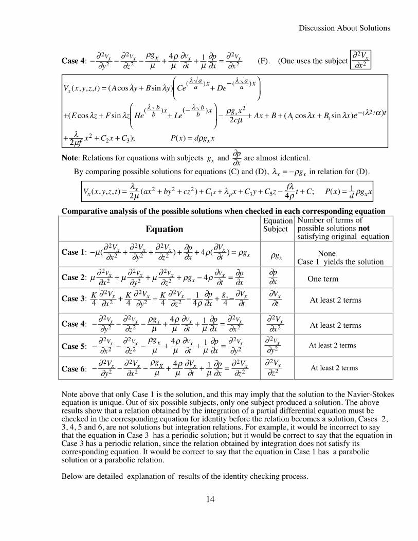
14

Case 4: − − − + + =∂∂

∂∂

ρμ

ρμ

∂∂ μ

∂∂

∂∂

2

2

2

2

2

24 1Vx Vx Vx Vx

y z

gxt

px x

(F). (One uses the subject ∂∂2

2Vx

x

V x y z t A y B y Cex

Dex

E z F z He Lex g x

c Ax B A x B x t

x

aa

aa

bb

x bb x e

( , , , ) ( cos sin )

( cos sin(

( cos sin ) )

( ) )

( ) )

(

( /

= + + −⎛

⎝⎜⎞

⎠⎟

+ + +−⎛

⎝⎜

⎞

⎠⎟ − + + + + −

+

λ λ

λ λ ρμ λ λ λ α

λ

λ λ

λ λ 22

2 1 1

222

2 3μ ρf x C x C P x d g xx+ + =) ( );

Note: Relations for equations with subjects gx and ∂∂px

are almost identical.

By comparing possible solutions for equations (C) and (D), λ ρx xg= − in relation for (D).

V x y z t ax by cz C x C y C zf

t C P x d g xxx x xp( , , , ) ( ) ( )= + + + + + + − + =λμ λ λ

ρ ρ2 412 2 2

51 3 ;

Comparative analysis of the possible solutions when checked in each corresponding equation

EquationEquationSubject

Number of terms ofpossible solutions notsatisfying original equation

Case 1: − + + + + =μ ∂∂

∂∂

∂∂

∂∂ ρ ∂

∂ ρ( ) ( )2

2

2

2

2

2 4Vx

Vy

Vz

px

Vt

gx x x xx ρgx

NoneCase 1 yields the solution

Case 2: μ ∂∂ μ ∂

∂ μ ∂∂ ρ ρ ∂

∂∂∂

2

2

2

2

2

2 4Vx Vx Vx

xVx

x y zg

tpx

+ + + − =

∂∂px One term

Case 3: K Vx

K Vy

K Vz

px

g Vt

x x x xx

4 4 41

4 42

2

2

2

2

2∂∂

∂∂

∂∂ ρ

∂∂

∂∂+ + − + =

∂∂Vtx At least 2 terms

Case 4: − − − + + =∂∂

∂∂

ρμ

ρμ

∂∂ μ

∂∂

∂∂

2

2

2

2

2

24 1Vx Vx x Vx Vx

y zg

tpx x

∂∂2

2Vx

x At least 2 terms

Case 5: − − − + + =∂∂

∂∂

ρμ

ρμ

∂∂ μ

∂∂

∂∂

2

2

2

2

2

24 1Vx Vx Vx Vx

x z

gxt

px y

∂∂

2

2Vx

y At least 2 terms

Case 6: − − − + + =∂∂

∂∂

ρμ

ρμ

∂∂ μ

∂∂

∂∂

2

2

2

2

2

24 1V

yVx

gx Vt

px

Vz

x x x x ∂∂2

2Vz

x At least 2 terms

Note above that only Case 1 is the solution, and this may imply that the solution to the Navier-Stokesequation is unique. Out of six possible subjects, only one subject produced a solution. The aboveresults show that a relation obtained by the integration of a partial differential equation must bechecked in the corresponding equation for identity before the relation becomes a solution, Cases 2,3, 4, 5 and 6, are not solutions but integration relations. For example, it would be incorrect to saythat the equation in Case 3 has a periodic solution; but it would be correct to say that the equation inCase 3 has a periodic relation, since the relation obtained by integration does not satisfy itscorresponding equation. It would be correct to say that the equation in Case 1 has a parabolicsolution or a parabolic relation.

Below are detailed explanation of results of the identity checking process.

Discussion About Solutions

15

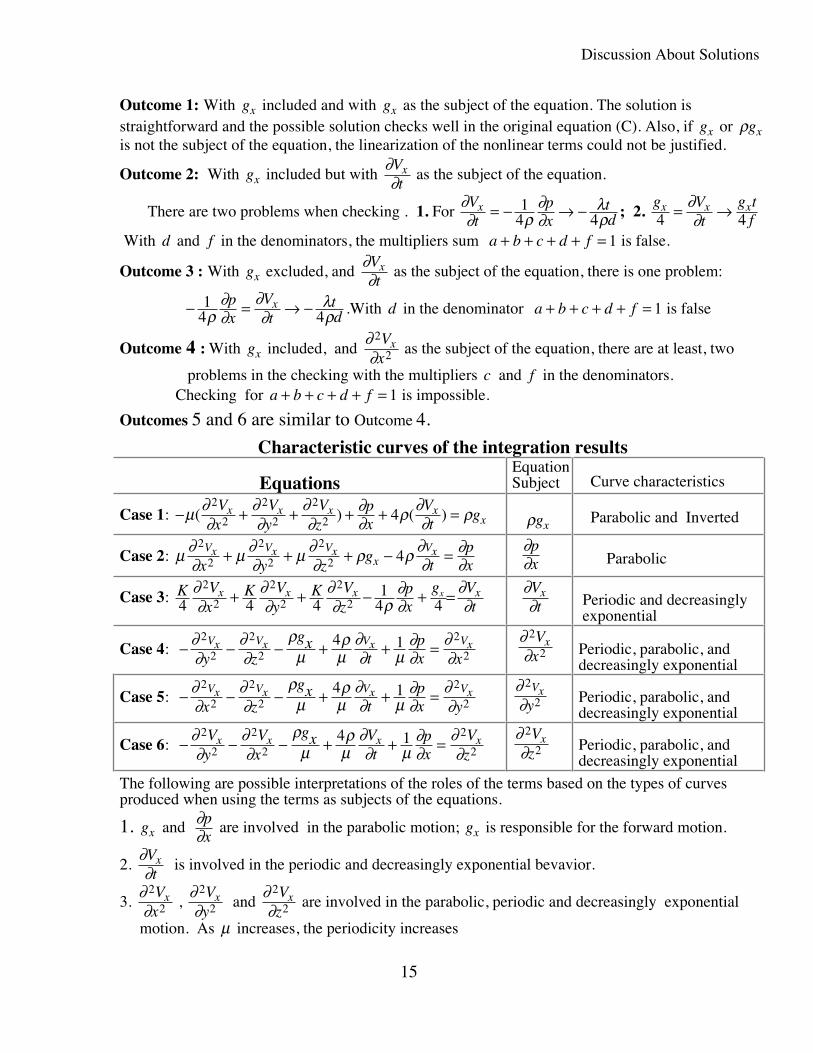
Outcome 1: With gx included and with gx as the subject of the equation. The solution isstraightforward and the possible solution checks well in the original equation (C). Also, if gx or ρgxis not the subject of the equation, the linearization of the nonlinear terms could not be justified.

Outcome 2: With gx included but with ∂∂Vtx as the subject of the equation.

There are two problems when checking . 1. For ∂∂ ρ

∂∂

λρ

Vt

px

td

x = − → −14 4 ; 2.

g Vt

g tf

x x x4 4= →∂

∂ With d and f in the denominators, the multipliers sum a b c d f+ + + + = 1 is false.

Outcome 3 : With gx excluded, and ∂∂Vtx as the subject of the equation, there is one problem:

− = → −14 4ρ

∂∂

∂∂

λρ

px

Vt

td

x .With d in the denominator a b c d f+ + + + = 1 is false

Outcome 4 : With gx included, and ∂∂2

2Vx

x as the subject of the equation, there are at least, two

problems in the checking with the multipliers c f and in the denominators. Checking for a b c d f+ + + + = 1 is impossible.

Outcomes 5 and 6 are similar to Outcome 4.

Characteristic curves of the integration results

EquationsEquationSubject Curve characteristics

Case 1: − + + + + =μ ∂∂

∂∂

∂∂

∂∂ ρ ∂

∂ ρ( ) ( )2

2

2

2

2

2 4Vx

Vy

Vz

px

Vt

gx x x xx ρgx

Parabolic and Inverted

Case 2: μ ∂∂ μ ∂

∂ μ ∂∂ ρ ρ ∂

∂∂∂

2

2

2

2

2

2 4Vx Vx Vx

xVx

x y zg

tpx

+ + + − =

∂∂px Parabolic

Case 3: K Vx

K Vy

K Vz

px

g Vt

x x x xx

4 4 41

4 42

2

2

2

2

2∂∂

∂∂

∂∂ ρ

∂∂

∂∂+ + − + =

∂∂Vtx Periodic and decreasingly

exponential

Case 4: − − − + + =∂∂

∂∂

ρμ

ρμ

∂∂ μ

∂∂

∂∂

2

2

2

2

2

24 1Vx Vx Vx Vx

y z

gxt

px x

∂∂2

2Vx

x Periodic, parabolic, anddecreasingly exponential

Case 5: − − − + + =∂∂

∂∂

ρμ

ρμ

∂∂ μ

∂∂

∂∂

2

2

2

2

2

24 1Vx Vx Vx Vx

x z

gxt

px y

∂∂

2

2Vx

y Periodic, parabolic, anddecreasingly exponential

Case 6: − − − + + =∂∂

∂∂

ρμ

ρμ

∂∂ μ

∂∂

∂∂

2

2

2

2

2

24 1V

yVx

gx Vt

px

Vz

x x x x ∂∂2

2Vz

x Periodic, parabolic, anddecreasingly exponential

The following are possible interpretations of the roles of the terms based on the types of curvesproduced when using the terms as subjects of the equations.

1. gx and ∂∂px

are involved in the parabolic motion; gx is responsible for the forward motion.

2. ∂∂Vtx is involved in the periodic and decreasingly exponential bevavior.

3. ∂∂2

2Vx

x , ∂∂2

2Vy

x and ∂∂2

2Vz

x are involved in the parabolic, periodic and decreasingly exponential

motion. As μ increases, the periodicity increases

Discussion About Solutions

16

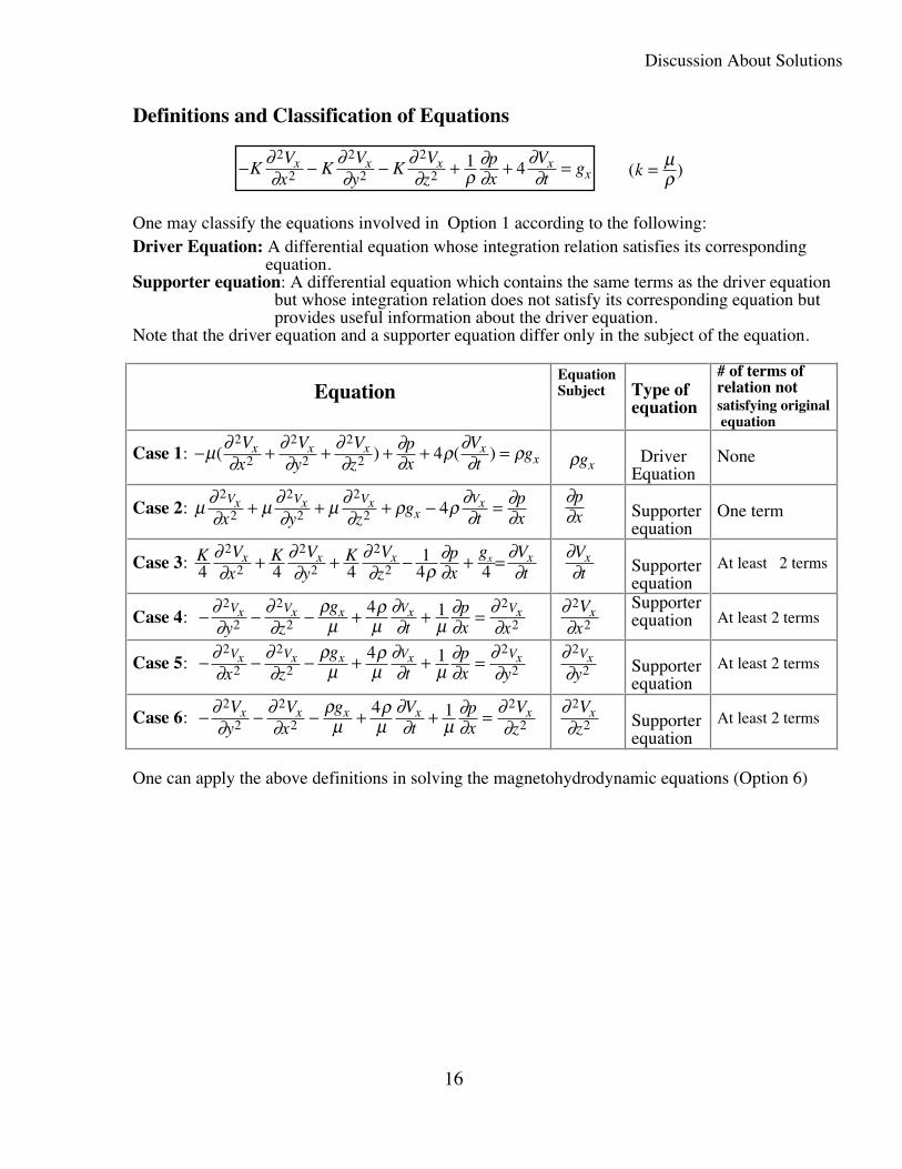
Definitions and Classification of Equations

− − − + + =KVx

KVy

KVz

px

Vt

gx x x xx

∂∂

∂∂

∂∂ ρ

∂∂

∂∂

2

2

2

2

2

21 4 (k = μ

ρ )

One may classify the equations involved in Option 1 according to the following:Driver Equation: A differential equation whose integration relation satisfies its corresponding equation.Supporter equation: A differential equation which contains the same terms as the driver equation but whose integration relation does not satisfy its corresponding equation but provides useful information about the driver equation.Note that the driver equation and a supporter equation differ only in the subject of the equation.

EquationEquationSubject Type of

equation

# of terms ofrelation notsatisfying original equation

Case 1: − + + + + =μ ∂∂

∂∂

∂∂

∂∂ ρ ∂

∂ ρ( ) ( )2

2

2

2

2

2 4Vx

Vy

Vz

px

Vt

gx x x xx ρgx

DriverEquation

None

Case 2: μ ∂∂ μ ∂

∂ μ ∂∂ ρ ρ ∂

∂∂∂

2

2

2

2

2

2 4Vx Vx Vx

xVx

x y zg

tpx

+ + + − = ∂∂px Supporter

equationOne term

Case 3: K Vx

K Vy

K Vz

px

g Vt

x x x xx

4 4 41

4 42

2

2

2

2

2∂∂

∂∂

∂∂ ρ

∂∂

∂∂+ + − + =

∂∂Vtx Supporter

equationAt least 2 terms

Case 4: − − − + + =∂∂

∂∂

ρμ

ρμ

∂∂ μ

∂∂

∂∂

2

2

2

2

2

24 1Vx Vx x Vx Vx

y zg

tpx x

∂∂2

2Vx

xSupporterequation At least 2 terms

Case 5: − − − + + =∂∂

∂∂

ρμ

ρμ

∂∂ μ

∂∂

∂∂

2

2

2

2

2

24 1Vx Vx x Vx Vx

x zg

tpx y

∂∂

2

2Vx

y Supporterequation

At least 2 terms

Case 6: − − − + + =∂∂

∂∂

ρμ

ρμ

∂∂ μ

∂∂

∂∂

2

2

2

2

2

24 1V

yVx

g Vt

px

Vz

x x x x x ∂∂2

2Vz

x Supporterequation

At least 2 terms

One can apply the above definitions in solving the magnetohydrodynamic equations (Option 6)

Discussion About Solutions

17

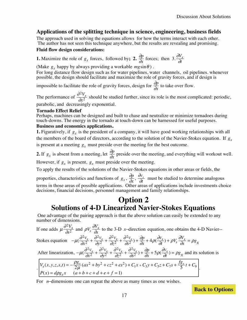
Applications of the splitting technique in science, engineering, business fieldsThe approach used in solving the equations allows for how the terms interact with each other. The author has not seen this technique anywhere, but the results are revealing and promising.Fluid flow design considerations:

1. Maximize the role of gx forces, followed by; 2. ∂∂px

forces; then 3.∂∂Vtx

(Make gx happy by always providing a workable mgsinθ ) .For long distance flow design such as for water pipelines, water channels, oil pipelines. wheneverpossible, the design should facilitate and maximize the role of gravity forces, and if design is

impossible to facilitate the role of gravity forces, design for ∂∂px

to take over flow.

The performance of ∂∂2

2Vx

x should be studied further, since its role is the most complicated: periodic,

parabolic, and decreasingly exponential.Tornado Effect ReliefPerhaps, machines can be designed and built to chase and neutralize or minimize tornadoes duringtouch-downs. The energy in the tornado at touch-down can be harnessed for useful purposes.Business and economics applications.1. Figuratively, if gx is the president of a company, it will have good working relationships with allthe members of the board of directors, according to the solution of the Navier-Stokes equation. If gx

is present at a meeting gx must preside over the meeting for the best outcome.

2. If gx is absent from a meeting, let ∂∂px

preside over the meeting, and everything will workout well.

However, if gx is present, gx must preside over the meeting.

To apply the results of the solutions of the Navier-Stokes equations in other areas or fields, the

properties, characteristics and functions of gx , ∂∂px

, ∂∂vtx must be studied to determine analogous

terms in those areas of possible applications. Other areas of applications include investments choicedecisions, financial decisions, personnel management and family relationships.

Option 2Solutions of 4-D Linearized Navier-Stokes Equations

One advantage of the pairing approach is that the above solution can easily be extended to anynumber of dimensions.

If one adds μ ∂∂2

2Vs

x and ρ ∂∂VVssx to the 3-D x−direction equation, one obtains the 4-D Navier--

Stokes equation − + + + + + + =μ ∂∂

∂∂

∂∂

∂∂

∂∂ ρ ∂

∂ ρ ∂∂ ρ( ) ( )

2

2

2

2

2

2

2

2 4Vx Vx Vx Vx Vx

sx

x y z spx t

VVs

gx

After linearization, − + + + + + =μ ∂∂

∂∂

∂∂

∂∂

∂∂ ρ ∂

∂ ρ( ) ( )2

2

2

2

2

2

2

2 5Vx Vx Vx Vx Vx

x y z spx t

gx and its solution is

. V x y z s t

gax by cz es C x C y C z C s

fgt C

P x d g x a b c d e f

x

x

x x( , , , , ) ( )

( )

= − + + + + + + + +

= + + + + + =

+ρ

μρ

2 51

2 2 2 21 3 5 7 9

( ) .

For n−dimensions one can repeat the above as many times as one wishes.

Back to Options

Solutions of the Euler Equations

18

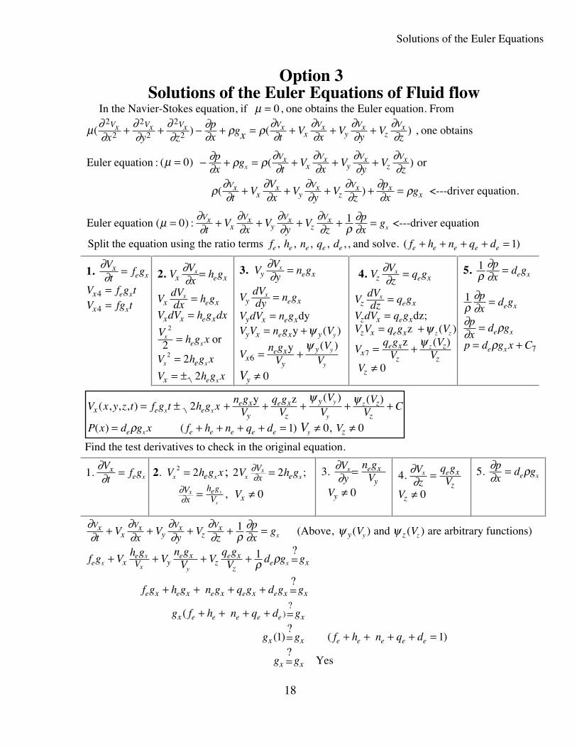
Option 3Solutions of the Euler Equations of Fluid flow

In the Navier-Stokes equation, if µ = 0, one obtains the Euler equation. From

µ ∂∂

∂∂

∂∂

∂∂ ρ ρ ∂

∂∂∂

∂∂

∂∂( ) ( )

2

2

2

2

2

2Vx Vx Vx Vx

xVx

yVx

zVx

x y zpx

gx tV

xV

yV

z+ + − + = + + + , one obtains

Euler equation : ( ) ( )µ ∂∂ ρ ρ ∂

∂∂∂

∂∂

∂∂= − + = + + +0 p

xg

tV

xV

yV

zx

Vxx

Vxy

Vxz

Vx or

ρ ∂∂

∂∂

∂∂

∂∂

∂∂ ρ( )

Vxx

xy

Vxz

Vx xxt

VVx

Vy

Vz

px

g+ + + + = <---driver equation.

Euler equation ( :µ ∂∂

∂∂

∂∂

∂∂ ρ

∂∂= + + + + =0 1)

Vxx

Vxy

Vxz

Vxt

Vx

Vy

Vz

px

gx <---driver equation

Split the equation using the ratio terms f h n q de e e e e, , , , , , and solve. ( )f h n q de e e e e+ + + + = 1

1. ∂∂Vt

f gxe x=

V f g tx e x4 =V fg tx x4 =

2. V Vx

h gx xx

e∂∂ =

VdVdx h g

V dV h g dxx x

x x x

xe

e

==

Vh g xx

xe

2

2 = or

V h g xx xe2 2=

V h g xx e x= ± 2

3. VVy

n gy xx

e∂∂ =

VdVdy n g

V dV n gV V n g V

Vn g

VV

V

y x

y x x

y x x y

xx

y

y

y

x

y

y

y

e

e

e

e

V

=

== +

= +

≠

dyy (

y

ψψ

)( )

6

0

4. V Vz

q gz xx

e∂∂ =

VdVdz q g

V dV q gV V q g V

Vq g

VV

VV

z x

z x x

z x x

xx

z

z

z

z

x

z z

z

e

e

e

e

==

= +

= +

≠

dz;z (

z

ψψ

)( )

7

0

5. 1ρ∂∂px

d ge x=

1

7

ρ∂∂

∂∂ ρ

ρ

px

d g

px

d g

p d g x C

e x

e x

e x

=

== +

V x y z t f g t h g xn g

Vq g

VV

VV

V C

P x d g x f h n q d V

xx

y

x

z

y z

z

z

e ee e

e e e e e e

x xy

y

z

x yV

( , , , )( ) ( )

( ) ( ) ,

= ± + + + + +

= + + + + = ≠ ≠

2

1 0 0

y z

ψ ψ

ρ

Find the test derivatives to check in the original equation.

1. ∂∂Vt

f gxe x= 2. V h g xx xe

2 2= ; 2 2V h gxx

xVx e

∂∂ = ;

∂∂Vx

hV

x egx

x

x

V= ≠, 0

3

0

.

∂∂Vy

n gV

V

x e x

y

y

=

≠4

0

. ∂∂Vz

q gV

V

x e x

z

z

=

≠

5. ∂∂ ρpx

d ge x=

∂∂

∂∂

∂∂

∂∂ ρ

∂∂ ψ ψ

ρ ρ

Vxx

Vxy

Vxz

Vxy z

x yx

zx

zx

tV

xV

yV

zpx

g V V

f g Vh g

Vn g

V Vq gV d g g

x y z

xx

x yxe

e e eeV

+ + + + =

+ + + + =

1

1

(Above, ( and ( are arbitrary functions)

) )

?

f g h g n g q g d g ge e e e ex x x x x x+ + + + = ?

g f h n q d gx xe e e e e( )?

+ + + + =

( g g f h n q dx x e e e e e( )?

)1 1= + + + + =

g gx x?= Yes

Solutions of the Euler Equations

19

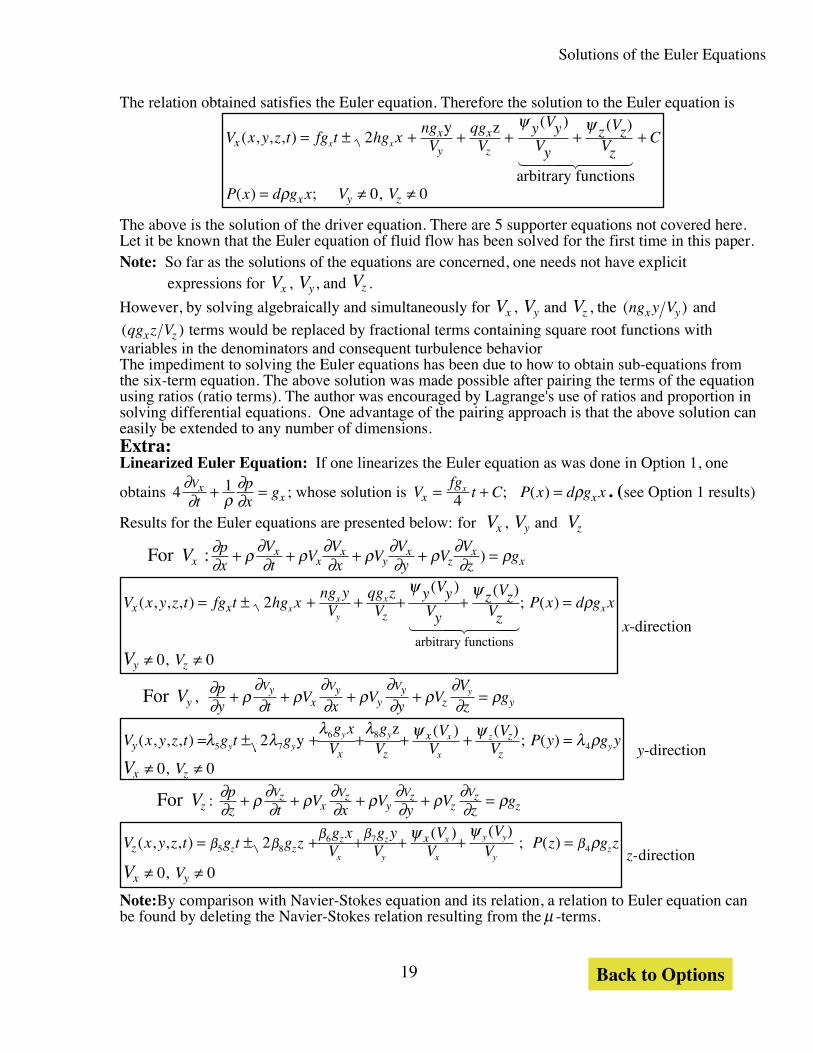
The relation obtained satisfies the Euler equation. Therefore the solution to the Euler equation is

V x y z t fg t hg xngV

qgV

y VyVy

z VzVz

C

P x d g x V V

xx

y

x

z

x y z

x x( , , , )( ) ( )

( ) ; ,

= ± + + + + +

= ≠ ≠

2

0 0

y z

arbitrary functions

ψ ψ

ρ

1 2444 3444

The above is the solution of the driver equation. There are 5 supporter equations not covered here.Let it be known that the Euler equation of fluid flow has been solved for the first time in this paper.Note: So far as the solutions of the equations are concerned, one needs not have explicit expressions for Vx , Vy, and Vz .

However, by solving algebraically and simultaneously for Vx , Vy and Vz , the ( )ng y Vx y and

( )qg z Vx z terms would be replaced by fractional terms containing square root functions withvariables in the denominators and consequent turbulence behaviorThe impediment to solving the Euler equations has been due to how to obtain sub-equations fromthe six-term equation. The above solution was made possible after pairing the terms of the equationusing ratios (ratio terms). The author was encouraged by Lagrange's use of ratios and proportion insolving differential equations. One advantage of the pairing approach is that the above solution caneasily be extended to any number of dimensions.Extra:Linearized Euler Equation: If one linearizes the Euler equation as was done in Option 1, one

obtains 4 1∂∂ ρ

∂∂

Vxxt

px

g+ = ; whose solution is Vfg

t C P x d g xx xx= + =4 ; ( ) ρ . (see Option 1 results)

Results for the Euler equations are presented below: for Vx , Vy and Vz

For Vx : ∂∂ ρ ∂

∂ ρ ∂∂ ρ ∂

∂ ρ ∂∂ ρp

xVt

VVx

VVy

VVz

gxx

xy

xz

xx+ + + + =)

V x y z t fg t hg xng yV

qg zV

y VyVy

z VzVz

P x d g x

V

x xz

y z

xx

y

xx

V

( , , , )( ) ( )

( )

,

= ± + + + + =

≠ ≠

2

0 0

ψ ψρ

arbitrary functions

;

1 2444 3444 x-direction

For Vy , ∂∂ ρ

∂∂ ρ

∂∂ ρ

∂∂ ρ

∂∂ ρp

y tV

xV

yV

Vz

gVy

xVy

yVy

z yy+ + + + =

V x y z t g t gg x

Vg

VV

VV

V P y g y

V

yx z

x z

z

x z

y yy y x

x

zy

V

( , , , )( ) ( )

( )

,

= ± + + + + =

≠ ≠

λ λλ λ ψ ψ λ ρ5 7

6 842

0 0

yz

;

y-direction

For Vz : ∂∂ ρ ∂

∂ ρ ∂∂ ρ ∂

∂ ρ ∂∂ ρp

z tV

xV

yV

zg

Vzx

Vzy

Vzz

Vzz+ + + + =

V x y z t g t g zg xV

g yV

VV

VV P z g z

V

zx

x y

zx

z

y

x

x

y y

yzz

z

V

( , , , )( ) ( )

( )

,

= ± + + + + =

≠ ≠

β ββ β

βψ ψ

ρ5 86 7

42

0 0

;

z-direction

Note:By comparison with Navier-Stokes equation and its relation, a relation to Euler equation canbe found by deleting the Navier-Stokes relation resulting from the μ -terms.

Back to Options

Solutions of the Navier-Stokes Equations (Original)

20

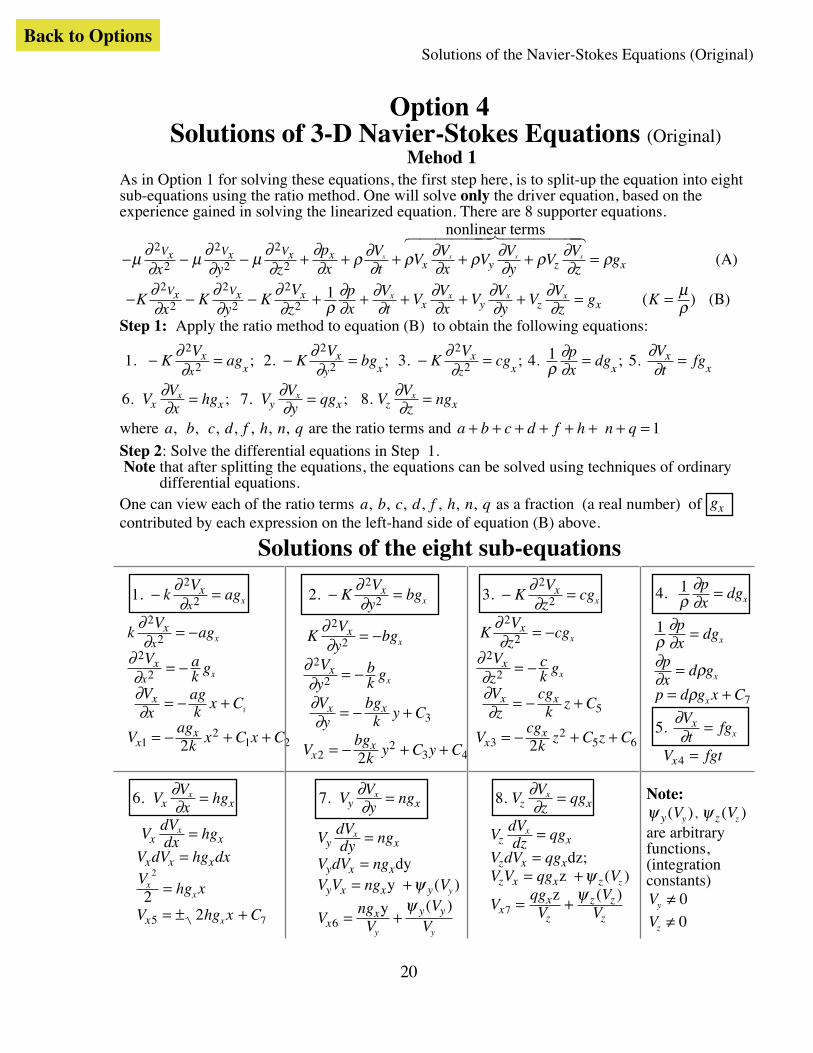
Option 4 Solutions of 3-D Navier-Stokes Equations (Original)

Mehod 1As in Option 1 for solving these equations, the first step here, is to split-up the equation into eightsub-equations using the ratio method. One will solve only the driver equation, based on theexperience gained in solving the linearized equation. There are 8 supporter equations.

− − − + + + + + =μ ∂∂ μ ∂

∂ μ ∂∂

∂∂ ρ ∂

∂ ρ ∂∂ ρ ∂

∂ ρ ∂∂ ρ

2

2

2

2

2

2Vx Vx Vx x

x y z xx y zpx

Vt

VVx

VVy

VVz

gx x x x

nonlinear terms6 744444 844444

(A)

− − − + + + + + = =Kx

Ky

KVz

px

Vt

VVx

VVy

VVz

g KVx Vx x

x y z xx x x x∂

∂∂∂

∂∂ ρ

∂∂

∂∂

∂∂

∂∂

∂∂

μρ

2

2

2

2

2

21 ( ) (B)

Step 1: Apply the ratio method to equation (B) to obtain the following equations:

1 1 52

2

2

2

2

2. . ; 2. ; 3. ; 4. ; − = − = − = = =KV

ag KV

bg KV

cgpx

dgVt

fgxx x

xy x

xz x x

xx

∂∂

∂∂

∂∂ ρ

∂∂

∂∂

6. ; V Vx

hgx xx∂

∂ = 7. ; VVy

qgy xx∂

∂ = 8. V Vz

ngz xx∂

∂ =

where a b c d f h n q, , , , , , , are the ratio terms and a b c d f h n q+ + + + + + + = 1

Step 2: Solve the differential equations in Step 1. Note that after splitting the equations, the equations can be solved using techniques of ordinary differential equations.One can view each of the ratio terms a b c d f h n q, , , , , , , as a fraction (a real number) of gx contributed by each expression on the left-hand side of equation (B) above.

Solutions of the eight sub-equations

12

2. − =kV

agxx x

∂∂

kV

ag

V ak g

Vx

agk x C

Vag

k x C x C

xx

xx

x

xx

x

x

∂∂

∂∂∂∂

2

22

2

12

1 2

1

2

= −

= −

= − +

= − + +

2. − =KVy

bgxx

∂∂2

2

KVy

bg

Vy

bk g

Vy

bgk y C

Vbg

k y C y C

x

x

x x

xx

x

x

∂∂

∂∂∂∂

2

2

2

2

3

22

3 42

= −

= −

= − +

= − + +

3. − =KVz

cgxx

∂∂2

2

KVz

cg

Vz

ck g

Vz

cgk z C

Vcg

k z C z C

x

x

x x

xx

x

x

∂∂

∂∂∂∂

2

22

2

5

32

5 62

= −

= −

= − +

= − + +

4 1. ρ∂∂px

dgx=

1

7

ρ∂∂

∂∂ ρ

ρ

px

dg

px

d g

p d g x C

x

x

x

=

== +

5. ∂∂Vt

fgxx=

V fgtx4 =

6. V Vx

hgx xx∂

∂ =

V dVdx hg

V dV hg dxV

hg x

V hg x C

x x

x x x

x

x

xx

x

==

=

= ± +

2

225 7

7. VVy

ngy xx∂

∂ =

VdVdy ng

V dV ngV V ng V

VngV

VV

y x

y x x

y x x y

xx y y

x

y

y y

=

== +

= +

dyy (

y

ψψ

)( )

6

8. V Vz

qgz xx∂

∂ =

VdVdz qg

V dV qgV V qg V

VqgV

VV

z x

z x x

z x x z

xx

z

z z

z

x

z

==

= +

= +

dz;z (

zψ

ψ)

( )7

Note:ψ y Vy( ), ψ z Vz( )are arbitraryfunctions,(integrationconstants)Vy ≠ 0

Vz ≠ 0

Back to Options

Solutions of the Navier-Stokes Equations (Original)

21

Step 3: One combines the above solutions

V x y z t V V V V V V Vag

k x C xbg

k y C ycg

k z C z fg t hg xng yV

qg zV

VV

VV

g

x x x x x x x x

xy z y

z z

z

x

x x xx

x x y y

( , , , )( ) ( )

= + + + + + +

= − + − + − + ± + + + +

−

+

1 2 3 4 5 6 7

21

23

252 2 2 2

ψ ψ

ρ22 22 2 2

1 3 5µψ ψ

( )( ) ( )

ax by cz C x C y C z fg t hg xng y qg z V V

x xx

y

x

z

z

zV V V Vy y

y

z+ + + + + + ± + + + +

relation for linear terms relation for non - linear terms

arbitrary functions

6 7444444444 8444444444

1 244 344

6 74444444 844444444

+

= + + + + + + + = ≠ ≠

C

P x d g x a b c d f h n qx V Vy z

9

1 0 0( ) ; ( ) ,ρ

Step 4: Find the test derivatives Test derivatives for the linear part Test derivatives for the non-linear part

∂∂

ρµ

2

2Vxa g

x

x

=

−

∂∂ρµ

2

2Vyb g

x

x

=

−

∂∂ρµ

2

2Vx

zc gx

=

−

∂∂ρ

px

d gx

= ∂∂Vt

fg

x

x

=V hg xx x

2 2=

2 2V hgxx

xVx

∂∂ =

∂∂Vx

hgx

x

xxV V= ≠, 0

∂∂Vy

ngV

x x

y= ∂

∂Vz

qgV

x x

z=

Step 5: Substitute the derivatives from Step 4 in equation (A) for the checking.

− − − + + + + + =µ ∂∂ µ ∂

∂ µ ∂∂

∂∂ ρ ∂

∂ ρ ∂∂ ρ ∂

∂ ρ ∂∂ ρ

2

2

2

2

2

2Vx

Vy

Vz

px

Vt

VVx

VVy

VVz

gx x x xx y z x

x x x x (A)

− − − − + + + + + =

+ + + + + + + =

µ ρµ

ρµ

ρµ ρ ρ ρ ρ ρ ρ

ρ ρ ρ ρ ρ ρ ρ ρ ρ

( ) ( ) ( ) ( )?

?

a g b g c gd g f g V

hgV V

ngV V

qgV g

a g b g c g d g f g h g n g q g g

x x xx

x

x

x x x x

x x yx

yz

x

zx

x x x x xx

x x x x x

x x

x x

ag bg cg dg fg hg ng qg g

g a b c d f h n q g

g g a b c d f h n q

x x x x

Yes (

+ + + + + + +

+ + + + + + + =

= + + + + + + + =

=?

( )

( ) )

?

?1 1

Step 6: The linear part of the relation satisfies the linear part of the equation; and the non-linear part of the relation satisfies the non-linear part of the equation.(B) below is the solution.

Analogy for the Identity Checking Method: If one goes shopping with American dollars andJapanese yens (without any currency conversion) and after shopping, if one wants to check the costof the items purchased, one would check the cost of the items purchased with dollars against thereceipts for the dollars; and one would also check the cost of the items purchased with yens againstthe receipts for the yens purchase. However, if one converts one currency to the other, one wouldonly have to check the receipts for only a single currency, dollars or yens. This conversion case issimilar to the linearized equations, where there was no partitioning in identity checking.

Solutions of the Navier-Stokes Equations (Original)

22

Summary of solutions for Vx Vy, Vz ( P x d g xx( ) = ρ ; P y g yy( ) = λ ρ4 , P z g zz( ) = β ρ4 )V

V V

x

xx x

x

y

x

z

y y

y

z z

z

y z

gax by cz C x C y C z fg t hg x

ng yV

qg zV

VV

VV C

P x d g x a b c d h n qx

=

− + + + + + + ± + + + + +

= + + + + + + = ≠ ≠

ρμ

ψ ψ

ρ2 2

1 0 0

2 2 21 3 5 9( )

( ) ( )

( ) ; ( ) ,

(B)

Vg

x y z C x C y C z g t gg x

Vg

VV

VV

VP y g y

yx

y

z

x

x

z z

z

y

yy y

y x

x zV V

= − + + + + + + ± + + + +

= ≠ ≠

ρμ λ λ λ λ λ

λ λ ψ ψ

λ ρ2 2

0 0

12

22

32

1 3 5 5 76 8

4

( )( ) ( )

( ) ,

yz

Vg

x y z C x C y C z g t g zg x g y

zx

x

x

y

x y

zz

z

y

x y

yz

zV V

VV

V

V

V V

= − + + + + + ± + + + +

≠ ≠

+ρ

μ β β β β β β β ψ ψ2 2

0 0

1 2 3 5 86 72 2 2

1 3 5( )( ) ( )

,

The above solutions are unique, because from the experience in Option 1, only the equations withthe gravity terms as the subjects of the equations produced the solutions.

Option 5Solutions of 4-D Navier-Stokes Equations

In the above method, the solution can easily be extended to any number of dimensions..

Adding μ ∂∂2

2Vs

x and ρ ∂∂VVssx to the 3-D x−direction equation yields the 4-D N-S equation

− + + + + + + + + + =μ ∂∂

∂∂

∂∂

∂∂

∂∂ ρ ∂

∂ ρ ∂∂ ρ ∂

∂ ρ ∂∂ ρ ∂

∂ ρ( )2

2

2

2

2

2

2

2Vx

Vy

Vz

Vs

px

Vt

VVx

VVy

VVz

VVs

gx x x xx y z s

xx

x x x x

whose solution is given byV x y z s t

gax by cz es C x C y C z C s fg t hg x

ng yV

qg zV

rg sV

VV

VV

VV

x

xx x

x

y

x

z s

y y

y

z z

z

s s

s

x

( , , , , )

( )

( ) ( ) ( )

=

− + + + + + + + + ± + + + +

+ +

ρμ

ψ ψ ψ2 22 2 2 2

1 3 5 6

arbitrary functions1 244444 34444

+

= + + + + + + + + + = ≠ ≠ ≠

C

P x d g x a b c d e f h n q rx x y sV V V

9

1 0 0 0

( ) ( ) , , ,ρ

For n−dimensions one can repeat the above as many times as one wishes.

Option 5bTwo-term Linearized Navier-Stokes Equation (one nonlinear term)

By linearization as in Option 1, if one replaces ρ ∂∂ ρ ∂

∂VVy

VVzy z

x x+ by 2ρ ∂∂Vt

x in

− − − + + + + + =μ ∂∂ μ ∂

∂ μ ∂∂

∂∂ ρ ∂

∂ ρ ∂∂ ρ ∂

∂ ρ ∂∂ ρ

2

2

2

2

2

2Vx Vx Vx x

x y z xx y zpx

Vt

VVx

VVy

VVz

gx x x x one obtains

− + + + + + + =μ ∂∂

∂∂

∂∂

∂∂

∂∂ ρ ∂

∂ ρ ∂∂ ρ( ) ( )

2

2

2

2

2

2

2

2 3Vx Vx Vx Vx Vx

xx y z spx t

VVx

gxx , whose solution is

Vg

ax by cz C x C y C zfg t

hg x Cx x y z t xx

x( , , , ) ( )= − + + + + + + ± +ρμ2 3 22 2 2

1 3 5 6

Back to Options

Back to Options

Conclusion :Solutions of the Navier-Stokes Equations

23

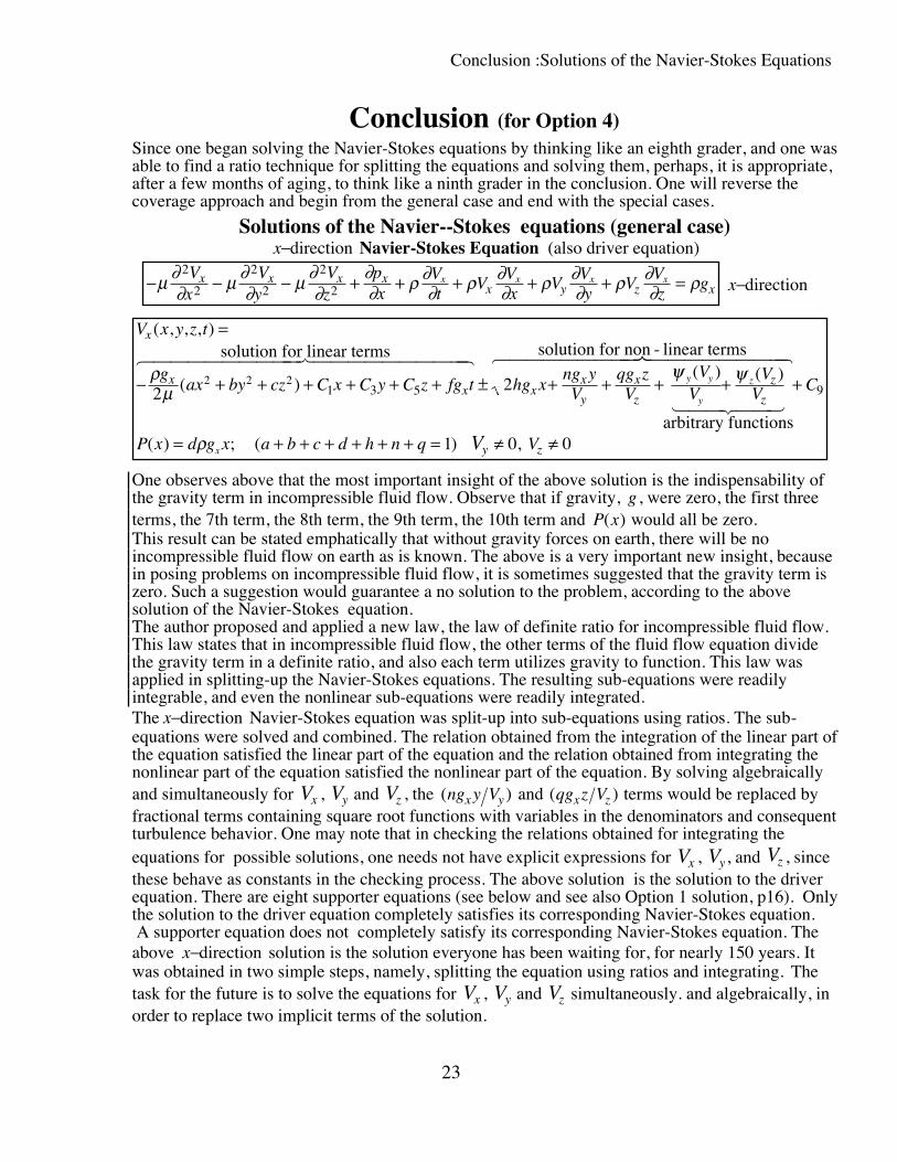
Conclusion (for Option 4)Since one began solving the Navier-Stokes equations by thinking like an eighth grader, and one wasable to find a ratio technique for splitting the equations and solving them, perhaps, it is appropriate,after a few months of aging, to think like a ninth grader in the conclusion. One will reverse thecoverage approach and begin from the general case and end with the special cases.

Solutions of the Navier--Stokes equations (general case)x−direction Navier-Stokes Equation (also driver equation)

− − − + + + + + =μ ∂∂ μ ∂

∂ μ ∂∂

∂∂ ρ ∂

∂ ρ ∂∂ ρ ∂

∂ ρ ∂∂ ρ

2

2

2

2

2

2Vx

Vy

Vz

px

Vt

VVx

VVy

VVz

gx x x xx y z x

x x x x x−direction

V x y z t

gax by cz C x C y C z fg t hg x

ng yV

qg zV

VV

VV

x

xx x

x

y

x

z

z

z

y y

y

z

( , , , )

( )( ) ( )

=

− + + + + + + ± + + + +ρμ

ψ ψ2 22 2 2

1 3 5

solution for linear terms

arbitrary functions

solution for non - linear terms6 7444444444 8444444444

1 244 344

6 7744444444 844444444

+

= + + + + + + = ≠ ≠

C

P x d g x a b c d h n q Vx Vy z

9

1 0 0( ) ; ( ) ,ρ

One observes above that the most important insight of the above solution is the indispensability ofthe gravity term in incompressible fluid flow. Observe that if gravity, g , were zero, the first threeterms, the 7th term, the 8th term, the 9th term, the 10th term and P x( ) would all be zero.This result can be stated emphatically that without gravity forces on earth, there will be noincompressible fluid flow on earth as is known. The above is a very important new insight, becausein posing problems on incompressible fluid flow, it is sometimes suggested that the gravity term iszero. Such a suggestion would guarantee a no solution to the problem, according to the abovesolution of the Navier-Stokes equation.The author proposed and applied a new law, the law of definite ratio for incompressible fluid flow.This law states that in incompressible fluid flow, the other terms of the fluid flow equation dividethe gravity term in a definite ratio, and also each term utilizes gravity to function. This law wasapplied in splitting-up the Navier-Stokes equations. The resulting sub-equations were readilyintegrable, and even the nonlinear sub-equations were readily integrated.The x−direction Navier-Stokes equation was split-up into sub-equations using ratios. The sub-equations were solved and combined. The relation obtained from the integration of the linear part ofthe equation satisfied the linear part of the equation and the relation obtained from integrating thenonlinear part of the equation satisfied the nonlinear part of the equation. By solving algebraicallyand simultaneously for Vx , Vy and Vz , the ( )ng y Vx y and ( )qg z Vx z terms would be replaced byfractional terms containing square root functions with variables in the denominators and consequentturbulence behavior. One may note that in checking the relations obtained for integrating theequations for possible solutions, one needs not have explicit expressions for Vx , Vy, and Vz , sincethese behave as constants in the checking process. The above solution is the solution to the driverequation. There are eight supporter equations (see below and see also Option 1 solution, p16). Onlythe solution to the driver equation completely satisfies its corresponding Navier-Stokes equation. A supporter equation does not completely satisfy its corresponding Navier-Stokes equation. Theabove x−direction solution is the solution everyone has been waiting for, for nearly 150 years. Itwas obtained in two simple steps, namely, splitting the equation using ratios and integrating. Thetask for the future is to solve the equations for Vx , Vy and Vz simultaneously. and algebraically, inorder to replace two implicit terms of the solution.

Conclusion :Solutions of the Navier-Stokes Equations

24

Supporter Equations

1

2

2

2

2

2

2

2

2

2

2

2

2

2

.

.

− − − + + + + + =

− − − +

μ ∂∂ μ ∂

∂ μ ∂∂

∂∂ ρ ∂

∂ ρ ∂∂ ρ ∂

∂ ρ ρ ∂∂

μ ∂∂ μ ∂

∂ μ ∂∂

∂∂

Vx

Vy

Vz

px

Vt

VVy

VVz

g VVx

Vx

Vy

Vz

px

x x x xy z x x

x x x x

x x x x

++ + + + =

− − − + + + + + =

−

ρ ∂∂ ρ ∂

∂ ρ ∂∂ ρ ρ ∂

∂

μ ∂∂ μ ∂

∂ μ ∂∂ ρ ∂

∂ ρ ∂∂ ρ ∂

∂ ρ ∂∂ ρ ∂

∂

VVx

VVy

VVz

gVt

Vx

Vy

Vz

Vt

VVx

VVy

VVz

gpx

x y z x

x x xx y z x

x

x x x x

x x x x3

4

2

2

2

2

2

2.

.

μμ ∂∂ μ ∂

∂∂∂ ρ ∂

∂ ρ ∂∂ ρ ∂

∂ ρ ∂∂ ρ μ ∂

∂2

2

2

2

2

2Vy

Vz

px

Vt

VVx

VVy

VVz

gVx

x x xx y z x

xx x x x− + + + + + + = −

Explicit Functions for Vx , Vy, and Vz ,For explicit functions for Vx , Vy, and Vz , one has to solve (algebraically) the simultaneous system

of solutions for Vx , Vy, and Vz .

System of Navier Stokes relations to solve for simultaneously −=

− + + + + + + ± + + + +

=

− +

V V VV

gax by cz C x C y C z fg t hg x V V qg V V ng V V

V VV

gx

x y z

x

z x x z

y z

y

xx x y z z y y y

y

, ,

( ( ) [ ( ( )

( (

) z )] [ y ]

(algebraically).

ρμ ψ ψ

ρμ λ λ

2 2

2

2 2 21 3 5

12

222

32

1 3 5 5 7 8 6

12

22

32

1 3 5

2

2

y z C x C y C z g t g g g x

V VV

gx y z C x C y C z

y y x z z x xV V V V V Vz y x y z

x z

z

z

+ + + + + ± + + + +

=

− + + + + +

λ λ λ λ ψ λ ψ

ρμ β β β

) [ ( ) [ ( )]

( ( )

y ) z ]

++ ± + + + +β β β ψ β ψ5 826 7

g t g z g x g y

V V

z z x y

x y

V V V V V Vz x x y z y y x) [ ( )] [ ( )]

Special Cases of the Navier-Stokes Equations1. Linearized Navier--Stokes equationsOne may note that there are six linear terms and three nonlinear terms in the Navier-Stokesequation. The linearized case was covered before the general case, and the experience gained in thelinearized case guided one to solve the general case efficiently. In particular, the gravity term mustbe the subject of the equation for a solution. When the gravity term was the subject of the equation,the equation was called the driver equation. A splitting technique was applied to the linearizedNavier-Stokes equations (Option 1). Twenty sub-equations were solved. (Four sets of equationswith different equation subjects). The integration relations of one of the sets satisfied the linearizedNavier-Stokes equation; and this set was from the equation with gx as the subject of the equation.In addition to finding a solution, the results of the integration revealed the roles of the terms of theNavier-Stokes equations in fluid flow. In particular, the gravity forces and ∂ ∂p x are involved

mainly in the parabolic as well as the forward motion of fluids; ∂ ∂V tx and ∂ ∂2 2Vx x are involvedin the periodic motion of fluids, and one may infer that as μ increases, the periodicity increases.One should determine experimentally, if the ratio of the linear term ∂ ∂V tx to the nonlinear sumV V x V V y V V zx x y x z x( ) ( ) ( )∂ ∂ ∂ ∂ ∂ ∂+ + is 1 to 3.

Back to Options

Conclusion :Solutions of the Navier-Stokes Equations

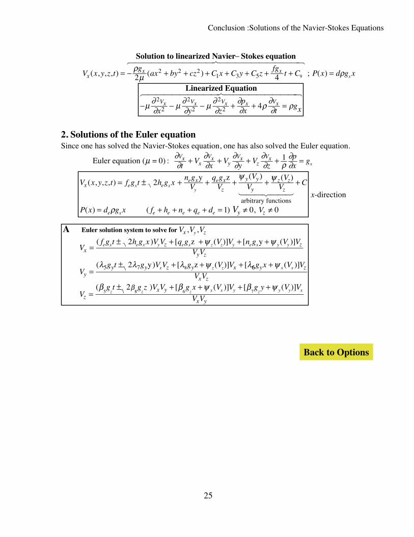
25

V x y z tg

ax by cz C x C y C zfg

t C P x d g xxx x

x( , , , ) ( ) ( )= − + + + + + + +

−

=ρμ ρ2 4

2 2 21 3 5 9 ;

Solution to linearized Navier Stokes equation6 74444444444 84444444444

− − − + + =μ ∂∂ μ ∂

∂ μ ∂∂

∂∂ ρ ∂

∂ ρ2

2

2

2

2

2 4Vx Vx Vx x Vx

x y zpx t

gx

Linearized Equation6 7444444444 8444444444

2. Solutions of the Euler equationSince one has solved the Navier-Stokes equation, one has also solved the Euler equation.

Euler equation ( = 0) : μ ∂∂

∂∂

∂∂

∂∂ ρ

∂∂

Vxx

Vxy

Vxz

Vxt

Vx

Vy

Vz

px

gx+ + + + =1

V x y z t f g t h g x

n gV

q gV

VV

VV C

P x d g x f h n q d V

xx x

z

y y

y

z z

z

y z

e ee e

e e e e e e

x xy

x V

( , , , )( ) ( )

( ) ( ) ,

= ± + + + + +

= + + + + = ≠ ≠

2

1 0 0

y z

arbitrary functions

ψ ψ

ρ

1 244 344 x-direction

A Euler solution system to solve for

) z )] [ y ]

y ) z ]

V V V

Vf g t h g x V V q g V V n g V V

V V

Vg t g V V g V V

x z

xz z

y z

yy y z y x

y

e x e x y e x z z y e x y y

x z z

, ,

( [ ( ( )

( [ ( ) [

=± + + + +

=± + + +

2

25 7 8

ψ ψ

λ λ λ ψ λ66

5 8 6 72

g x V V

V V

Vg t g z V V g x V V g y V V

V V

y z

x z

zx y

x y

x x

z z z x x y z y y x

+

=± + + + +

ψ

β β ψ β ψβ

( )]

( [ ( )] [ ( )]

)

Back to Options

Solutions of the Magnetohydrodynamic Equations

26

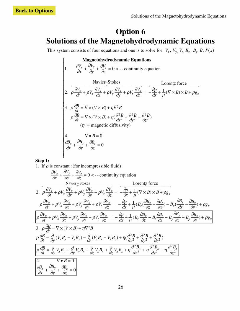
Option 6Solutions of the Magnetohydrodynamic EquationsThis system consists of four equations and one is to solve for V V V B B B P xx y z x y, , , , , , ( )

Magnetohydrodynamic Equations

1. < - - continuity equation

2.

Navier Stokes

Lorentz force

∂∂

∂∂

∂∂

ρ ∂∂ ρ ∂

∂ ρ ∂∂ ρ ∂

∂∂∂ μ ρ

Vx

Vy

Vz

Vt

VVx

VVy

VVz

px

B B g

x y z

xx

xy

xz

xx

+ + =

+ + +

−

= − + ∇ × × +

0

16 74444444 84444444 6 744444 8444

( )

444

3

4 0

0

2

22

22

22

. ( )

( ) ( )

(

.

magnetic diffusivity)

ρ ∂∂ η

ρ ∂∂ η ∂

∂∂∂

∂∂

η

∂∂

∂∂

∂∂

Bt

V B B

Bt

V B Bx

By

Bz

BBx

By

Bz

x y z

= ∇ × × + ∇

= ∇ × × + + +

=

∇ • =

+ + =

⎧

⎨

⎪⎪⎪⎪⎪⎪⎪⎪⎪⎪

⎩

⎪⎪⎪⎪⎪⎪⎪⎪⎪⎪⎪

Step 1:1. If is constant : (for incompressible fluid)

< - - continuity equation

2.

Lorentz forceNavier - Stokes

ρ∂∂

∂∂

∂∂

ρ ∂∂ ρ ∂

∂ ρ ∂∂ ρ ∂

∂∂∂ μ ρ

Vx

Vy

Vz

Vt

VVx

VVy

VVz

px

B B g

x y z

xx

xy

xz

xx

+ + =

+ + + = − + ∇ × × +

0

16 74444444 84444444 6 74444

( )

44 844444

ρ ∂∂ ρ ∂

∂ ρ ∂∂ ρ ∂

∂∂∂ μ

∂∂

∂∂

∂∂

∂∂ ρV

tV

Vx

VVy

VVz

px

BBz

Bx

BBx

By

gxx

xy

xz

xz

x zy

y xx+ + + = − + − − − +1 ( ( ) ( )

ρ ∂∂ ρ ∂

∂ ρ ∂∂ ρ ∂

∂∂∂ μ

∂∂

∂∂

∂∂

∂∂ ρV

tV

Vx

VVy

VVz

px

BBz

BBx

BBx

BBy

gxx

xy

xz

xz

xz

zy

yy

xx+ + + = − + − − + + 1 ( )

3 2

22

22

22

. ( )

( ) ( ) ( )

ρ ∂∂ η

ρ ∂∂

∂∂

∂∂ η ∂

∂∂∂

∂∂

Bt

V B B

Bt y

V B V Bz

V B V B Bx

By

Bzx y y x z x x z

= ∇ × × + ∇

= − − − + + +

ρ ∂∂

∂∂

∂∂

∂∂

∂∂ η ∂

∂ η ∂∂ η ∂

∂Bt y

V By

V Bz

V Bz

V BB

xB

yBzx y y x z x x z

x x x= − − + + + +2

2

2

2

2

2

4 0

0

. ∇ • =

+ + =

BBx

By

Bz

x y z∂∂

∂∂

∂∂

Back to Options

Solutions of the Magnetohydrodynamic Equations

27

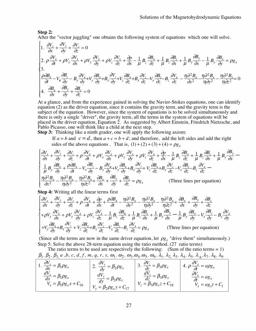
Step 2:After the "vector juggling" one obtains the following system of equations which one will solve.

1 0

2 1 1 1 1

3

.

.

.

∂∂

∂∂

∂∂

ρ ∂∂ ρ ∂

∂ ρ ∂∂ ρ ∂

∂∂∂ μ

∂∂ μ

∂∂ μ

∂∂ μ

∂∂ ρ

ρ∂∂

Vx

Vy

Vz

Vt

VVx

VVy

VVz

px

BBz

BBx

BBx

BBy

g

Bt

V

x y z

xx

xy

xz

xz

xz

zy

yy

xx

x

+ + =

+ + + + − + + − =

− xx yx

yx

x zx

xz

xz

zx x x x

x y z

By

BVy

VBy

BVy

VBz

BVz

VBz

BVz

Bx

By

Bz

Bx

By

Bz

y y∂∂

∂∂

∂∂

∂∂

∂∂

∂∂

∂∂

∂∂

η∂∂

η∂η∂

η∂η∂

∂∂

∂∂

∂∂

− + + + + − − − − − =

+ + =

⎧

2

2

2

2

2

2 0

4 0.

⎨⎨

⎪⎪⎪⎪⎪

⎩

⎪⎪⎪⎪⎪At a glance, and from the experience gained in solving the Navier-Stokes equations, one can identifyequation (2) as the driver equation, since it contains the gravity term, and the gravity term is thesubject of the equation. However, since the system of equations is to be solved simultaneously andthere is only a single "driver", the gravity term, all the terms in the system of equations will beplaced in the driver equation, Equation 2. As suggested by Albert Einstein, Friedrich Nietzsche, andPablo Picasso, one will think like a child at the next step.Step 3: Thinking like a ninth grader, one will apply the following axiom: If and a b= c d a c b d= + = +, then ; and therefore, add the left sides and add the right sides of the above equations . That is, ( ) ( ) ( ) ( )1 2 3 4+ + + = ρgx

∂∂

∂∂

∂∂ ρ ∂

∂ ρ ∂∂ ρ ∂

∂ ρ ∂∂

∂∂ μ

∂∂ μ

∂∂ μ

∂∂

μ∂∂

ρ∂∂

∂∂

∂

Vx

Vy

Vz

Vt

VVx

VVy

VVz

px

BBz

BBx

BBx

BBy

Bt

VBy

BV

x y z xx

xy

xz

xz

xz

zy

y

yx x

x yy

+ + + + + + + − + +

+ − −

−1 1 1

1 xxy

xx z

xx

zx

zz

x

x x x x y zx

yV

By

BVy

VBz

BVz

VBz

BVz

Bx

By

Bz

Bx

By

Bz

g

y

∂∂∂

∂∂

∂∂

∂∂

∂∂

∂∂

η∂∂

η∂η∂

η∂η∂

∂∂

∂∂

∂∂ ρ

+ + + + − −

− − + + + =

⎧

⎨

⎪⎪⎪

⎩

⎪⎪⎪

−2

2

2

2

2

2 (Three lines per equation)

Step 4: Writing all the linear terms first

∂∂

∂∂

∂∂ ρ ∂

∂∂∂

ρ∂∂

η∂∂

η∂η∂

η∂η∂

∂∂

∂∂

∂∂

ρ ∂∂ ρ ∂

∂ ρ ∂∂ μ

∂

Vx

Vy

Vz

Vt

px

Bt

Bx

By

Bz

Bx

By

Bz

VVx

VVy

VVz

BB

x y z x x x x x x y z

xx

yx

zx

z

+ + + + + − − − + + +

+ + + −

2

2

2

2

2

2

1 xxz

zy

yy

xx y

x

yx

x zx

xz

xz

zx

x

zB

Bx

BBx

BBy

VBy

BVy

VBy

BVy

VBz

BVz

VBz

BVz

g

y

y

∂ μ∂∂ μ

∂∂ μ

∂∂

∂∂

∂∂

∂∂

∂∂

∂∂

∂∂

∂∂

∂∂ ρ

+ + − −

+ + + + − − =

⎧

⎨

⎪⎪⎪

⎩

⎪⎪⎪

−1 1 1

(Three lines per equation)

(Since all the terms are now in the same driver equation, let ρgx "drive them" simultaneously.)Step 5: Solve the above 28-term equation using the ratio method. (27 ratio terms) The ratio terms to be used are respectively the following: (Sum of the ratio terms = 1)β β β ω ω ω ω ω ω λ λ λ λ λ λ λ λ λ1 2 3 1 2 3 4 5 6 1 2 3 4 5 6 7 8 9, , , , , , , , , , , , , , , , ,, , , , , , , , , a b c d f m q r s

1 1

1

1 16

.

∂∂ β ρ

β ρβ ρ

Vx

g

dVdx g

V g x C

x

x

x

x

x x

=

== +

2 2

2

2 17

.

∂∂ β ρ

β ρ

β ρ

Vy

g

dVdy g

V g y C

y

y

x

x

y x

=

=

= +

3 3

3

3 18

.

∂∂ β ρ

β ρβ ρ

Vz

g

dVdz g

V g z C

z

z

x

x

z x

=

== +

4

1

. ρ ∂∂ ρ

∂∂

Vt

a g

Vt

ag

V ag t C

xx

xx

x x

=

== +

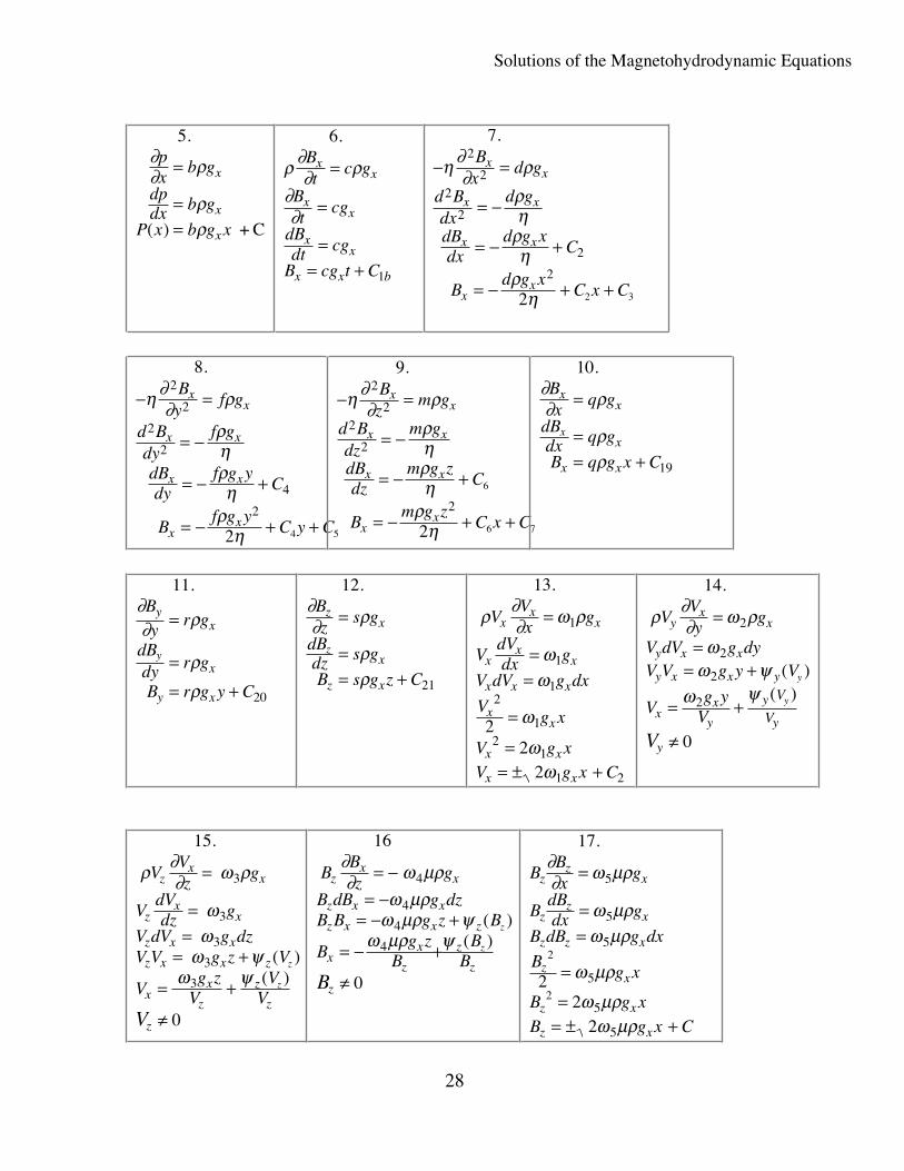
Solutions of the Magnetohydrodynamic Equations

28

5.

( )

+ C

∂∂ ρ

ρρ

px

b g

dpdx b g

P x b g x

x

x

x

=

==

6

1

.

ρ ∂∂ ρ

∂∂

Bt

c g

Bt

cg

dBdt cg

B cg t C

xx

xx

xx

x x b

=

=

== +

7

2

2

22

2

2

2

2 3

.

− =

= −

= − +

= − + +

η ∂∂ ρ

ρη

ρη

ρη

Bx

d g

d Bdx

d g

dBdx

d g xC

Bd g x

C x C

xx

x x

x x

xx

8

2

2

2

2

2

4

2

4 5

.

− =

= −

= − +

= − + +

η ∂∂ ρ

ρηρη

ρη

By

f g

d Bdy

f g

dBdy

f g yC

Bf g y

C y C

xx

x x

x x

xx

9

2

2

22

2

2

6

6 7

.

− =

= −

= − +

= − + +

η ∂∂ ρ

ρηρη

ρη

Bz

m g

d Bdz

m g

dBdz

m g zC

Bm g z

C x C

xx

x x

x x

xx

10

19

.∂∂ ρ

ρρ

Bx

q g

dBdx q g

B q g x C

xx

x

x x

x

=

== +

11

20

.∂∂ ρ

ρρ

By

r g

dBdy r g

B r g y C

yx

x

y x

y

=

=

= +

12

21

.∂∂ ρ

ρρ

Bz

s g

dBdz s g

B s g z C

zx

x

z x

z

=

== +

13

22

2

1

1

12

12

1

1 2

.

ρ ∂∂ ω ρ

ωω

ω

ωω

VVx

g

VdVdx g

V dV g dx

Vg x

V g xV g x C

xx

x

xx

x

x x x

xx

x x

x x

=

==

=

== ± +

14.

((

ρ ∂∂ ω ρ

ωω ψ

ω ψ

VVy

g

V dV g dyV V g y V

Vg y

V

yx

x

y x x

y x x y

xx

y

y

y

y

y

yV

V

V

=

== +

= +

≠

2

2

2

2

0

))

15.

((

ρ ∂∂ ω ρ

ωω

ω ψω ψ

VVz

g

VdVdz g

V dV g dzV V g z V

Vg z

VV

V

zx

x

zx

x

z x x

z x x z

xx

z

z

z

z

z

z

V

=

==

= +

= +

≠

3

3

3

3

3

0

))

((

16

0

4

4

4

4

BBz

g

B dB g dzB B g z B

Bg z

BB

B

zx

x

z x x

z x x z

xx

z

z

z

z

z

z

B

∂∂ ω μρ

ω μρω μρ ψ

ω μρ ψ

= −= −

= − +

= − +

≠

))

17

22

2

5

5

5

5

5

5

2

2

.

BBx

g

BdBdx g

B dB g dx

Bg x

B g x

B g x C

zz

x

zz

x

z z x

zx

z x

z x

∂∂ ω μρ

ω μρω μρ

ω μρ

ω μρω μρ

=

==

=

== ± +

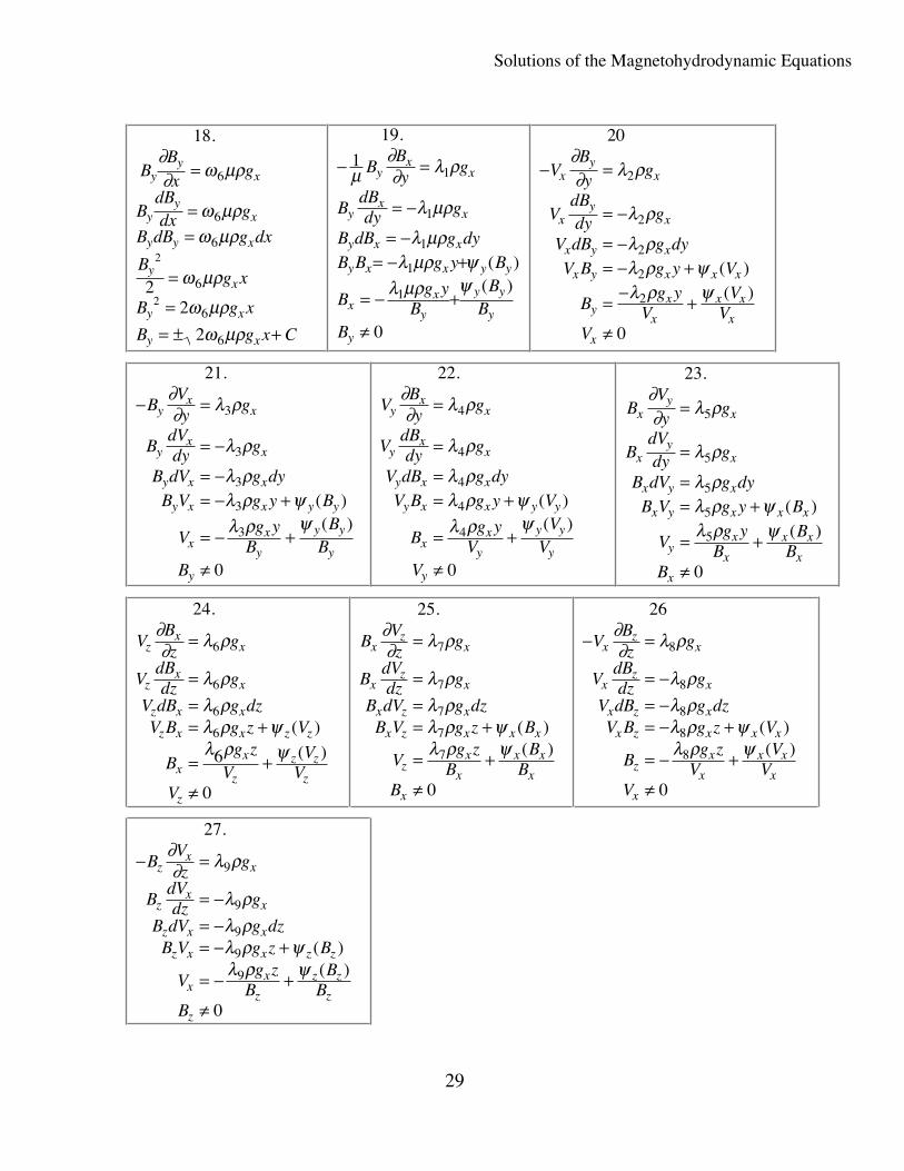
Solutions of the Magnetohydrodynamic Equations

29

18

22

2

6

6

6

6

6

6

2

2

.

BBx

g

BdBdx g

B dB g dx

Bg x

B g x

B g x C

yy

x

yy

x

y y x

yx

y x

y x

∂∂ ω μρ

ω μρω μρ

ω μρ

ω μρω μρ

=

==

=

== ± +

((

19

1

0

1

1

1

1

1

.

))

− =

= −

= −= − +

= − +

≠

μ∂∂ λ ρ

λ μρ

λ μρλ μρ ψ

λ μρ ψ

BBy

g

BdBdy g

B dB g dyB B g y B

Bg y

BB

BB

yx

x

yx

x

y x x

y x x y y

xx

y

y y

y

y

20

0

2

2

2

2

2

− =

= −

= −= − +

= − +

≠

VBy

g

VdBdy g

V dB g dyV B g y V

Bg y

VV

VV

xy

x

xy

x

x y x

x y x x x

yx

x

x x

x

x

∂∂ λ ρ

λ ρ

λ ρλ ρ ψλ ρ ψ

((

))

21

0

3

3

3

3

3

.

))

− =

= −

= −= − +

= − +

≠

BVy

g

BdVdy g

B dV g dyB V g y B

Vg y

BB

BB

yx

x

yx

x

y x x

y x x y y

xx

y

y y

y

y

∂∂ λ ρ

λ ρ

λ ρλ ρ ψλ ρ ψ

((

22

0

4

4

4

4

4

.

))

VBy

g

VdBdy g

V dB g dyV B g y V

Bg y

VV

VV

yx

x

yx

x

y x x

y x x y y

xx

y

y y

y

y

∂∂ λ ρ

λ ρ

λ ρλ ρ ψλ ρ ψ

=

=

== +

= +

≠

((

23

0

5

5

5

5

5

.

))

BVy

g

BdVdy g

B dV g dyB V g y B

Vg y

BB

BB

xy

x

xy

x

x y x

x y x x x

yx

x

x x

x

x

∂∂ λ ρ

λ ρ

λ ρλ ρ ψλ ρ ψ

=

=

== +

= +

≠

((

24

6

0

6

6

6

6

.

)

)

VBz

g

VdBdz g

V dB g dzV B g z V

Bg z

VV

VV

zx

x

zx

x

z x x

z x x z z

xx

z

z z

z

z

∂∂ λ ρ

λ ρλ ρλ ρ ψλ ρ ψ

=

=== +

= +

≠

(

(

25

0

7

7

7

7

7

.

))

BVz

g

BdVdz g

B dV g dzB V g z B

Vg z

BB

BB

xz

x

xz

x

x z x

x z x x x

zx

x

x x

x

x

∂∂ λ ρ

λ ρλ ρλ ρ ψλ ρ ψ

=

=== +

= +

≠

(

(

26

0

8

8

8

8

8

− =

= −= −= − +

= − +

≠

VBz

g

VdBdz g

V dB g dzV B g z V

Bg z

VV

VV

xz

x

xz

x

x z x

x z x x x

zx

x

x x

x

x

∂∂ λ ρ

λ ρλ ρλ ρ ψλ ρ ψ

((

))

27

0

9

9

9

9

9

.

))

− =

= −= −= − +

= − +

≠

BVz

g

BdVdz g

B dV g dzB V g z B

Vg z

BB

BB

zx

x

zx

x

z x x

z x x z z

xx

z

z z

z

z

∂∂ λ ρ

λ ρλ ρλ ρ ψλ ρ ψ

((

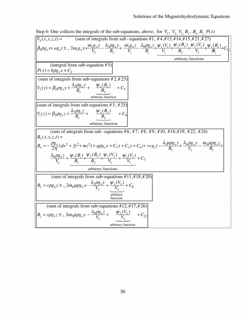
Solutions of the Magnetohydrodynamic Equations

30

Step 6: One collects the integrals of the sub-equations, above, for V V V B B B P xx y z x y z, , , , , , ( )

V x y z t

g x ag t g xg y

Vg y

Bg z

Vg z

BV

VB

BV

VB

x

x x xx

y

x

y

x

z

x

z

z z

z

y y

y

y y

y

z z

( , , , )) ) ) )

=

+ ± + − + − + + + +

(sum of integrals from sub - equations #1, # 4,#13,#14,#15,# 21,# 27)( ( ( ( β ρ ω ω λ ρ ω λ ρ ψ ψ ψ ψ

1 12 3 3 92 BB C

z

arbitrary functions1 2444444 3444444

+ 1 ;

(integral from sub equation #5)+

−=P x b g x Cx( ) ρ 2

(sum of integrals from sub equations # 2,# 23)(

arbitrary function

−

= + + +V y g yg y

BB

B Cy xx

x

x x

x( )

)β ρ λ ρ ψ2

53

124 34

(sum of integrals from sub equations #3, # 25)(

arbitrary function

−

= + + +V z g zg z

BB

B Cz xx

x

x x

x( )

)β ρ λ ρ ψ3

74

124 34

(sum of integrals from sub - equations #6, # 7, #8, # 9, #10, #16,#19, # 22, # 24)

B x y z t

Bg

dx fy mz q g x C x C y C z cg tg y

Bg y

Vg z

B

g zV

x

xx

x xx

y

x

y

x

z

x

( , , , )

( )

=

= − + + + + + + + + − + − +ρη ρ λ μρ λ ρ ω μρ

λ ρ2

2 2 2 1 4 4

6

2 4 6

zz

z

z

y y

y

y y

y

z z

z

BB

BB

VV

VV Cz

s

+ + + + +ψ ψ ψ ψ( ( ( (

arbitrary function

) ) ) )

1 2444444 34444447

(sum of integrals from sub equations #11,#18,# 20)(

arbitrary function

−

= ± − + +B r g y g xg y

VV

V Cy x xx

x

x x

xρ ω μρ λ ρ ψ

2 62

8)

124 34

(sum of integrals from sub equations #12,#17,# 26)(

arbitrary function

−

= ± − + +B s g z g xg z

VV

V Cz x xx

x

x x

xρ ω μρ λ ρ ψ

2 58

21)

124 34

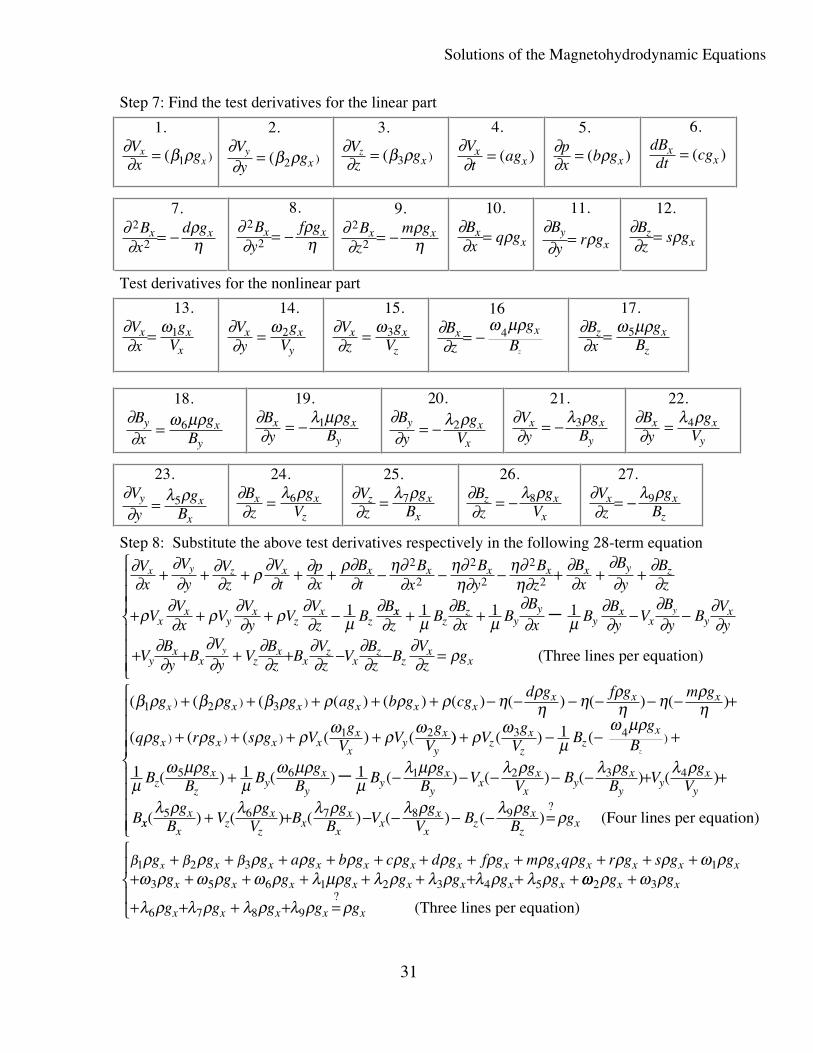
Solutions of the Magnetohydrodynamic Equations

31

Step 7: Find the test derivatives for the linear part

1

1

.

( )∂∂ β ρVx

gxx=

2

2

.

( )∂∂ β ρVy

gyx=

3. ∂∂ β ρVz

gzx= ( )3

4. ∂∂Vt

agxx= ( )

5.

( )

∂∂ ρpx

b gx=

6.

( )dBdt cgx

x=

72

2

.∂∂

ρη

Bx

d gx x= −

82

2

.∂∂

ρη

By

f gx x= −

92

2

.∂∂

ρη

Bz

m gx x= −

10.∂∂ ρBx

q gxx=

11.∂∂ ρBy

r gyx=

12.∂∂ ρBz

s gzx=

Test derivatives for the nonlinear part

13

1

.∂∂

ωVx

gV

x x

x=

14. ∂∂

ωVy

gV

x x

y= 2

15. ∂∂

ωVz

gV

x x

z= 3

16

4∂∂

ω μρBz

gB

x x

z

= −

17

5

.∂∂

ω μρBx

gB

z x

z=

18

6

.∂∂

ω μρBx

gB

y x

y=

19

1

.∂∂

λ μρBy

gB

x x

y= −

20

2

.∂∂

λ ρBy

gV

y x

x= −

21

3

.∂∂

λ ρVy

gB

x x

y= −

22

4

.∂∂

λ ρBy

gV

x x

y=

23

5

.∂∂

λ ρVy

gB

y x

x=

24

6

.∂∂

λ ρBz

gV

x x

z=

25

7

.∂∂

λ ρVz

gB

z x

x=

26

8

.∂∂

λ ρBz

gV

z x

x= −

27

9

.∂∂

λ ρVz

gB

x x

z= −

Step 8: Substitute the above test derivatives respectively in the following 28-term equation

∂∂

∂∂

∂∂ ρ ∂

∂∂∂

ρ∂∂

η∂∂

η∂η∂

η∂η∂

∂∂

∂∂

∂∂

ρ ∂∂ ρ ∂

∂ ρ ∂∂ μ

∂

Vx

Vy

Vz

Vt

px

Bt

Bx

By

Bz

Bx

By

Bz

VVx

VVy

VVz

BB

x y z x x x x x x y z

xx

yx

zx

z

+ + + + + − − − + + +

+ + + −

2

2

2

2

2

2

1 xxz

zy

yy

xx y

x

yx

x zx

xz

xz

zx

x

zB

Bx

BBx

BBy

VBy

BVy

VBy

BVy

VBz

BVz

VBz

BVz

g

y

y

∂ μ∂∂ μ

∂∂ μ

∂∂

∂∂

∂∂

∂∂

∂∂

∂∂

∂∂

∂∂

∂∂ ρ

+ + − −

+ + + + − − =

⎧

⎨

⎪⎪⎪

⎩

⎪⎪⎪

−1 1 1

(Three lines per equation)

( ( ( ( ) ( ) ( ) ( ) ( ) ( )

( ( ( ( ) (

) ) )

) ) )

β ρ β ρ β ρ ρ ρ ρ η ρη η ρ

η η ρη

ρ ρ ρ ρ ω ρ ω1 2 3

1 2

g g g ag b g cgd g f g m g

q g r g s g Vg

V Vg

V

x x x x x xx x x

x x x xx

xy

x

y

+ + + + + − − − − − − +

+ + + + )) ( ) (

( ) ( ) ( ) ( ) ( ) ( )

)+ − − +

+ − − − − − + +−

ρ ωμ

ω μρ

μω μρ

μω μρ

μλ μρ λ ρ λ ρ λ ρ

Vg

V Bg

B

Bg

B Bg

B Bg

B Vg

V Bg

B Vg

V

B

zx

zz

x

zx

zy

x

yy

x

yx

x

xy

x

yy

x

y

z

3 4

5 6 1 2 3 4

1

1 1 1

xxx

xz

x

zx

x

xx

x

xz

x

zx

gB V

gV B

gB V

gV B

gB g( ) ( ) ( ) ( ) ( )

?λ ρ λ ρ λ ρ λ ρ λ ρ ρ5 6 7 8 9+ + − − − − =

⎧

⎨

⎪⎪⎪⎪

⎩

⎪⎪⎪⎪ (Four lines per equation)

β β βρ ρ ρ ρ ρ ρ ρ ρ ρ ρ ρ ρ ω ρω ρ ω ρ ω ρ λ μρ λ ρ λ ρ λ ρ λ ρ1 2 3 1

3 5 6 1 2 3 4 5

g g g a g b g c g d g f g m g q g r g s g gg g g g g g g g

x x x x x x x x x x x x x

x x x x x x x x

+ + + + + + + + + + ++ + + + + + + + + ωω ρ ω ρ

λ ρ λ ρ λ ρ λ ρ ρ2 3

6 7 8 9

g g

g g g g g

x x

x x x x x

+

+ + + + =

⎧

⎨⎪

⎩⎪ ?

(Three lines per equation)

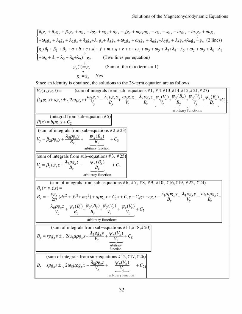
Solutions of the Magnetohydrodynamic Equations

32

β β β ω ω ω

ω λ λ λ λ λ ω ω λ λ λ λ1 2 3 1 3 5

6 1 2 3 4 5 2 3 6 7 8 9

g g g ag bg cg dg fg mg qg rg sg g g g

g g g g g g g g g g g

x x x x x x x x x x x x x x x

x x x x x x x x x x x

+ + + + + + + + + + + + +

+ + + + + + + + + + + + gg gx x=

⎧⎨⎩

? (2 lines)

g a b c d f m q r s

g

x

x

(?

)

β β β ω ω ω λ λ λ ω ω λ λ

ω λ λ λ λ1 2 3 1 3 5 3 4 5 2 3 6 7

6 1 2 8 9

+ + + + + + + + + + + + + + + + + + + + +

+ + + + + =

⎧⎨⎪

⎩⎪ (Two lines per equation)

g gx x( )?

1 = (Sum of the ratio terms = 1)

g gx x=?

Yes

Since an identity is obtained, the solutions to the 28-term equation are as follows

V x y z t

g x ag t g xg y

Vg y

Bg z

Vg z

BV

VB

BV

VB

x

x x xx

y

x

y

x

z

x

z

z z

z

y y

y

y y

y

z z

( , , , )) ) ) )

=

+ ± + − + − + + + +

(sum of integrals from sub - equations #1, # 4,#13,#14,#15,# 21,# 27) ( ( ( ( β ρ ω ω λ ρ ω λ ρ ψ ψ ψ ψ

1 12 3 3 92 BB C

z

arbitrary functions1 2444444 3444444

+ 1 ;

(integral from sub equation #5)+

−=P x b g x Cx( ) ρ 2

(sum of integrals from sub equations # 2,# 23)(

arbitrary function

−

= + + +V g yg y

BB

B Cy xx

x

x x

xβ ρ λ ρ ψ

25

3)

124 34

(sum of integrals from sub equations #3, # 25)(

arbitrary function

−

= + + +V g zg z

BB

B Cz xx

x

x x

xβ ρ λ ρ ψ

37

4)

124 34

(sum of integrals from sub - equations #6, # 7, #8, # 9, #10, #16,#19, # 22, # 24)

B x y z t

Bg

dx fy mz q g x C x C y C z cg tg y

Bg y

Vg z

B

g zV

x

xx

x xx

y

x

y

x

z

x

( , , , )

( )

=

= − + + + + + + + + − + − +ρη ρ λ μρ λ ρ ω μρ

λ ρ2

2 2 2 1 4 4

6

2 4 6

zz

z

z

y y

y

y y

y

z z

z

BB

BB

VV

VV Cz

s

+ + + + +ψ ψ ψ ψ( ( ( (

arbitrary function

) ) ) )

1 2444444 34444447

(sum of integrals from sub equations #11,#18,# 20)(

arbitrary function

−

= ± − + +B r g y g xg y

VV

V Cy x xx

x

x x

xρ ω μρ λ ρ ψ

2 62

8)

124 34

(sum of integrals from sub equations #12,#17,# 26)(

arbitrary function

−

= ± − + +B s g z g xg z

VV

V Cz x xx

x

x x

xρ ω μρ λ ρ ψ

2 58

21)

124 34

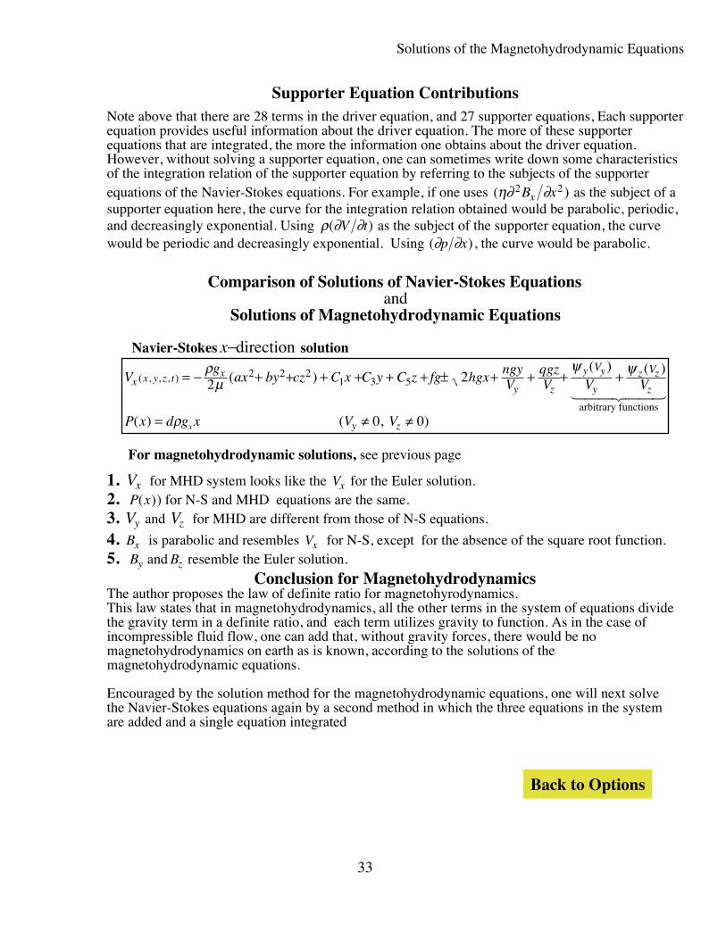
Solutions of the Magnetohydrodynamic Equations

33

Supporter Equation ContributionsNote above that there are 28 terms in the driver equation, and 27 supporter equations, Each supporterequation provides useful information about the driver equation. The more of these supporterequations that are integrated, the more the information one obtains about the driver equation.However, without solving a supporter equation, one can sometimes write down some characteristicsof the integration relation of the supporter equation by referring to the subjects of the supporterequations of the Navier-Stokes equations. For example, if one uses ( )η∂ ∂2 2B xx as the subject of asupporter equation here, the curve for the integration relation obtained would be parabolic, periodic,and decreasingly exponential. Using ρ ∂ ∂( )V t as the subject of the supporter equation, the curvewould be periodic and decreasingly exponential. Using ( )∂ ∂p x , the curve would be parabolic.

Comparison of Solutions of Navier-Stokes Equationsand

Solutions of Magnetohydrodynamic Equations

Navier-Stokes x−direction solution

Vg

ax by cz C x C y C z fg hgxngyV

qgzV V V

P x d g x V V

x x y z t x

y z

y y

y

z z

z

y z

V V

x

( , , , ) ( )( ) ( )

( )

= − + + + + + + ± + + + +

= ≠ ≠

ρμ

ψ ψ

ρ

2 22 2 21 3 5

arbitrary functions

( 0, 0)

1 244 344

For magnetohydrodynamic solutions, see previous page

1. Vx for MHD system looks like the Vx for the Euler solution.2. P x( )) for N-S and MHD equations are the same.3. Vy and Vz for MHD are different from those of N-S equations.

4. Bx is parabolic and resembles Vx for N-S, except for the absence of the square root function.5. By and Bz resemble the Euler solution.

Conclusion for MagnetohydrodynamicsThe author proposes the law of definite ratio for magnetohyrodynamics.This law states that in magnetohydrodynamics, all the other terms in the system of equations dividethe gravity term in a definite ratio, and each term utilizes gravity to function. As in the case ofincompressible fluid flow, one can add that, without gravity forces, there would be nomagnetohydrodynamics on earth as is known, according to the solutions of themagnetohydrodynamic equations.

Encouraged by the solution method for the magnetohydrodynamic equations, one will next solvethe Navier-Stokes equations again by a second method in which the three equations in the systemare added and a single equation integrated

Back to Options

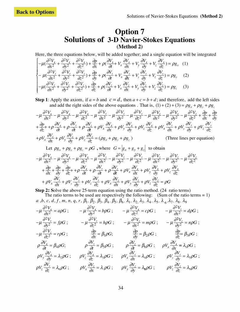
Solutions of Navier-Stokes Equations (Method 2)

34

Option 7Solutions of 3-D Navier-Stokes Equations

(Method 2)Here, the three equations below, will be added together; and a single equation will be integrated

− + + + + + + + =

− + + + + +

μ ∂∂

∂∂

∂∂

∂∂ ρ ∂

∂∂∂

∂∂

∂∂ ρ

μ∂∂

∂∂

∂∂

∂∂ ρ

∂∂

∂

( ) ( )

( ) (

2

2

2

2

2

2

2

2

2

2

2

2

Vx

Vy

Vz

px

Vt

VVx

VVy

VVz

g

Vx

Vy

Vz

py

Vt

VV

x x x xx

xy

xz

x

x

x

y y y y y

(1)

∂∂∂∂

∂∂ ρ

μ ∂∂

∂∂

∂∂

∂∂ ρ ∂

∂∂∂

∂∂

∂∂ ρ

xV

Vy

VVz

g

Vx

Vy

Vz

pz

Vt

VVx

VVy

VVz

g

yy y

y

z

z

z z z zx

zy

zz

z

+ + =

− + + + + + + + =

⎧

⎨

⎪⎪⎪

⎩

⎪⎪⎪

)

( ) ( )

(2)

(3) 2

2

2

2

2

2

Step 1: Apply the axiom, if and a b= c d a c b d= + = +, then ; and therefore, add the left sides and add the right sides of the above equations . That is, ( ) ( ) ( )1 2 3+ + = + +ρ ρ ρg g gx y z

− − − − − − − − − + +

+ + + + +

μ ∂∂ μ ∂

∂ μ ∂∂ μ

∂∂ μ

∂∂ μ

∂∂ μ ∂

∂ μ ∂∂ μ ∂

∂∂∂

∂∂

∂∂ ρ ∂

∂ ρ∂∂ ρ ∂

∂

2

2

2

2

2

2

2

2

2

2

2

2

2

2

2

2

2

2Vx

Vy

Vz

Vx

Vy

Vz

Vx

Vy

Vz

px

py

pz

Vt

Vt

V

x x x z z z

x z

y y y

y

ttV

Vx

VVy

VVz

VVx

VVy

VVz

VVx

VVy

VVz

g g g

xx

yx

zx

x z

xz

yz

zz

yy

y y

y zx

+ + + + + +

+ + + = + +

ρ ∂∂ ρ ∂

∂ ρ ∂∂ ρ

∂∂ ρ

∂∂ ρ

∂∂

ρ ∂∂ ρ ∂

∂ ρ ∂∂ ρ ρ ρ( ) (Three lines per equation)

Let ρ ρ ρ ρg g g Gx y z+ + = , where G g g gx y z= + + to obtain

− − − − − − − − −

+ + + + + + +

μ ∂∂ μ ∂

∂ μ ∂∂ μ

∂∂ μ

∂∂ μ

∂∂ μ ∂

∂ μ ∂∂ μ ∂

∂∂∂

∂∂

∂∂ ρ ∂

∂ ρ∂∂ ρ ∂

2

2

2

2

2

2

2

2

2

2

2

2

2

2

2

2

2

2Vx

Vy

Vz

Vx

Vy

Vz

Vx

Vy

Vz

px

py

pz

Vt

Vt

V

x x x z z z

x z

y y y

y ∂∂ ρ ∂∂ ρ ∂

∂ ρ ∂∂

ρ∂∂ ρ

∂∂ ρ

∂∂ ρ ∂

∂ ρ ∂∂ ρ ∂

∂ ρ

tV

Vx

VVy

VVz

VVx

VVy

VVz

VVx

VVy

VVz

G

xx

yx

zx

x z xz

yz

zzy

yy y

+ + +

+ + + + + + =

Step 2: Solve the above 25-term equation using the ratio method. (24 ratio terms) The ratio terms to be used are respectively the following: (Sum of the ratio terms = 1)a b c d f m n q r , , , , , , , , , , , , , , , , , , , , , , ,β β β β β β λ λ λ λ λ λ λ λ λ1 2 3 4 5 6 1 2 3 4 5 6 7 8 9

− = − = − = − =

− = − = − = −

μ ∂∂ ρ μ ∂

∂ ρ μ ∂∂ ρ μ

∂∂ ρ

μ∂∂ ρ μ

∂∂ ρ μ ∂

∂ ρ μ ∂

2

2

2

2

2

2

2

2

2

2

2

2

2

2

Vx

a GVy

b GVz

c GV

xd G

Vy

f GVz

h GV

xm G

x x x

z

y

y y

; ; ; ;

; ; ;22

2

2

2 1 2 3

4 5 6

Vy

n G

Vz

r Gpx

Gpy

Gpz

G

Vt

GVt

GVt

G VVx

z

z

x zx

xy

∂ ρ

μ ∂∂ ρ ∂

∂ β ρ ∂∂ β ρ ∂

∂ β ρ

ρ ∂∂ β ρ ρ

∂∂ β ρ ρ ∂

∂ β ρ ρ ∂∂

=

− = = = =

= = =

;

; ;

; ;

; ; ; ==

= = = =

= = =

λ ρ

ρ ∂∂ λ ρ ρ ∂

∂ λ ρ ρ∂∂ λ ρ ρ

∂∂ λ ρ

ρ∂∂ λ ρ ρ ∂

∂ λ ρ ρ ∂∂ λ

1

2 3 4 5

6 7

G

VVy

G VVz

G VVx

G VVy

G

VVz

G VVx

G VVy

yx

zx

x

z xz

yz

yy

y

y

;

;

; ; ;

; ; 88 9ρ ρ ∂∂ λ ρG VVz

Gzz ; =

Back to Options

Solutions of Navier-Stokes Equations (Method 2)

35

1∂∂ μ ρ

∂∂ μ ρ

μ ρ

2

2

1

2

1 22

Vx

a G

Vx

a Gx C

V a G x C x C

x

x

x

= −

= − +

= − + +

2

− =

= −

= − +

= − + +

μ ∂∂ ρ

∂∂ μ ρ

∂∂ μ ρ

μ ρ

2

2

2

2

3

2

3 42

Vy

b G

Vy

b G

Vy

b Gy C

V b Gy

C y C

x

x

x

x

3

− =

− =

= −

= − +

= − + +

μ ∂∂ ρ

μ ∂∂ ρ

∂∂ μ ρ

∂∂ μ ρ

μ ρ

2

22

22

2

5

2

5 62

Vz

c G

Vz

c G

Vz

c G

Vz

c Gz C

V c G z C z C

x

x

x

x

x

4

− =

− =

= −

= − +

= − + +

μ∂∂ ρ

μ∂∂ ρ

∂∂ μ ρ

∂∂ μ ρ

μ ρ

2

22

22

2

7

2

7 82

Vx

d G

Vx

d G

Vx

d G

Vx

d Gx C

V d G x C x C

y

y

y

y

y

5

− =

= −

= − +

= − + +

μ∂∂ ρ

∂∂ μ ρ

∂∂ μ ρ

μ ρ

2

2

2

2

9

2

9 102

Vy

f G

Vy

fG

Vy

fGy C

Vf

Gy

C y C

y

y

y

y

6

− =

= −

= − +

= − + +

μ∂∂ ρ

∂∂ μ ρ

∂∂ μ ρ

μ ρ

2

22

2

11

2

11 122

Vz

h G

Vz

h G

Vz

h Gz C

V h G z C z C

y

y

y

y

7

− =

= −

= − +

= − + +

μ ∂∂ ρ

∂∂ μ ρ

∂∂ μ ρ

μ ρ

2

22

2

13

2

13 142

Vx

m G

Vx

m G

Vx

m Gx C

V m G x C x C

z

z

z

z

8

− =

= −

= − +

= − + +

μ ∂∂ ρ

∂∂ μ ρ

∂∂ μ ρ

μ ρ

2

2

2

2

15

2

15 162

Vy

n G

Vy

n G

Vy

n Gy C

V m Gy

C y C

z

z

z

z

9

− =

= −

= − +

= − + +

μ ∂∂ ρ

∂∂ μ ρ

∂∂ μ ρ

μ ρ

2

22

2

17

2

17 182

Vz

r G

Vz

r G

Vz

r Gz C

V r G z C z C

z

z

z

z

10∂∂ β ρ

β ρβ ρ

px

G

dpdx G

P x Gx C

=

== +

1

1

1 19

( )

11∂∂ β ρ

β ρ

β ρ

py

G

dpdy G

P y Gy C

=

=

= +

2

2

2 20

( )

12∂∂ β ρ

β ρβ ρ

pz

G

dpdz G

P z Gz C

=

== +

3

3

3 21

( )

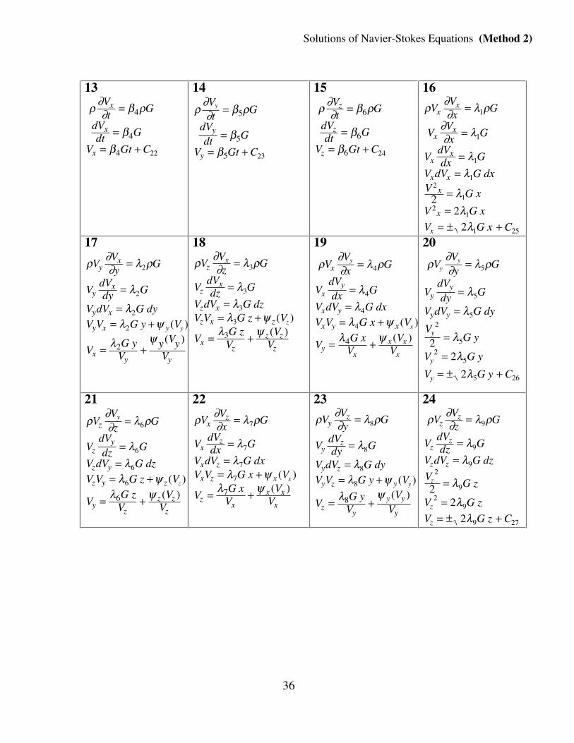
Solutions of Navier-Stokes Equations (Method 2)

36

13

ρ ∂∂ β ρ

ββ

Vt

G

dVdt G

V Gt C

x

x

x

=

== +

4

4

4 22

14

ρ∂∂ β ρ

ββ

Vt

G

dVdt G

V Gt C

y

y

y

=

== +

5

5

5 23

15

ρ ∂∂ β ρ

ββ

Vt

G

dVdt G

V Gt C

z

z

z

=

== +

6

6

6 24

16

ρ ∂∂ λ ρ

∂∂ λ

λλ

λλ

λ

VVx

G

VVx

G

VdVdx G

V dV G dxV G x

V G x

V G x C

xx

xx

xx

x x

x

x

x

=

=

==

==

= ± +

1

1

1

12

1

21

1 25

22

2

17

ρ ∂∂ λ ρ

λ

λλ ψ

λ ψ

VVy

G

VdVdy G

V dV G dyV V G y V

VG y

Vy VyV

yx

yx

y x

y x y

xy y

y

=

=

== +

= +

2

2

2

2

2

(

()

)

18

ρ ∂∂ λ ρ

λλ

λ ψλ ψ

VVz

G

VdVdz G

V dV G dzV V G z V

VG zV

VV

zx

zx

z x

z x z

xz

z z

z

z

=

==

= +

= +

3

3

3

3

3

(

()

)

19

(

(

ρ∂∂ λ ρ

λλ

λ ψλ ψ

VVx

G

VdVdx G

V dV G dxV V G x V

VG x

VV

V

x

xy

x y

x y x

yx

x x

x

y

x

=

==

= +

= +

4

4

4

4

4

))

20

ρ∂∂ λ ρ

λ

λ

λ

λλ

VVy

G

VdVdy G

V dV G dy

VG y

V G y

V G y C

yy

yy

y y

y

y

y

=

=

=

=

== ± +

5

5

52

5

25

5 26

22

2

21

ρ∂∂ λ ρ

λλ

λ ψλ ψ

VVz

G

VdVdz G

V dV G dzV V G z V

VG z

VV

V

z

zy

z y

z y z

yz

z z

z

y

z

=

==

= +

= +

6

6

6

6

6

(

()

)

22

ρ ∂∂ λ ρ

λλ

λ ψλ ψ

VVx

G

VdVdx G

V dV G dxV V G x V

VG x

VV

V

xz

xz

x z

x z x

zx

x x

x

x

=

==

= +

= +

7

7

7

7

7

(

()

)

23

ρ ∂∂ λ ρ

λ

λλ ψ

λ ψ

VVy

G

VdVdy G

V dV G dyV V G y V

VG y

VV

V

yz

yz

y z

y z y

zy

y y

y

y

=

=

== +

= +

8

8

8

8

8

(

()

)

24

ρ ∂∂ λ ρ

λλ

λ

λλ

VVz

G

VdVdz G

V dV G dz

VG z

V G z

V G z C

zz

zz

z z

z

z

z

=

==

=

== ± +

9

9

92

9

29

9 27

22

2

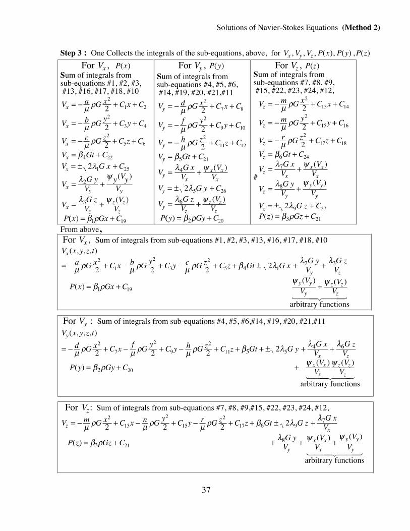
Solutions of Navier-Stokes Equations (Method 2)

37

Step 3 : One Collects the integrals of the sub-equations, above, for V V V P x P y P zx y z, , , ( ), ( ) , ( )

For Vx , P x( )Sum of integrals fromsub-equations #1, #2, #3, #13, #16, #17, #18, #10

V a G x C x C

V b Gy

C y C

V c G z C z C

V Gt C

V G x C

VG y

Vy VyV

VG zV

VV

P

x

x

x

x

xy y

xz

z z

z

x

= − + +

= − + +

= − + +

= += ± +

= +

= +

μ ρ

μ ρ

μ ρ

βλ

λ ψ

λ ψ

2

1 2

2

3 4

2

5 6

22

1 25

2

2

2

24

2

3

(

(

)

)

(( )x Gx C= +β ρ1 19

For Vy , P y( )Sum of integrals fromsub-equations #4, #5, #6, #14, #19, #20, #21,#11

V d G x C x C

Vf

Gy

C y C

V h G z C z C

V Gt C

VG x

VV

V

V G y C

VG z

VV

VP

y

y

y

y

yx

x x

x

yz

z z

z

y

= − + +

= − + +

= − + +

= +

= +

= ± +

= +

μ ρ

μ ρ

μ ρ

βλ ψ

λλ ψ

2

7 8

2

9 10

2

11 12

21

5 26

2

2

2

2

5

4

6

(

(

)

)

(( ) y Gy C= +β ρ2 20

For Vz , P z( )Sum of integrals fromsub-equations #7, #8, #9, #15, #22, #23, #24, #12,

#

V m G x C x C

V m Gy

C y C

V r G z C z C

V Gt C

VG x

VV

V

VG y

VV

V

V G z CP

z

z

z

z

zx

x x

x

zy

y y

y

z

= − + +

= − + +

= − + +

= +

= +

= +

= ± +

μ ρ

μ ρ

μ ρ

βλ ψ

λ ψ

λ

2

13 14

2

15 16

2

17 18

24

9 27

2

2

2

2

6

7

8

(

(

(

)

)

zz Gz C) = +β ρ3 21

From above, For Vx , Sum of integrals from sub-equations #1, #2, #3, #13, #16, #17, #18, #10V x y z t

a G x C x b Gy

C y c G z C z Gt G xG y

VG zV

P x Gx CV

VV

V

x

y z

y y

y

z z

z

( , , , )

) )

= − + − + − + + ± + +

= + +

μ ρ μ ρ μ ρ β λ λ λ

β ρψ ψ

2

1

2

3

2

5 1

19

2 2 2 242 3

1

( ) ( (

arbitrary functions1 24444 3444

For Vy : Sum of integrals from sub-equations #4, #5, #6,#14, #19, #20, #21,#11

V x y z t

d G x C xf

Gy

C y h G z C z Gt G yG x

VG z

V

P y Gy CV

VV

V

y

x z

x x

x

z z

z

( , , , )

) )

= − + − + − + + + ± + +

= + +

μ ρ μ ρ μ ρ β λ λ λ

β ρ ψ ψ

2

7

2

9

2

11 5

20

2 2 2 254 6

2

( ) ( (

arbitrary functions1 2444 344

For Vz : Sum of integrals from sub-equations #7, #8, #9,#15, #22, #23, #24, #12,

V m G x C x n Gy

C y r G z C z Gt G zG x

V

P z Gz CG y

VV

VV

V

zx

y

x x

x

y y

y

= − + − + − + + ± +

= + + + +

μ ρ μ ρ μ ρ β λ λ

β ρ λ ψ ψ

2

13

2

15

2

17 9

21

2 2 2 267

38

( ) ( (

arbitrary functions

) )

1 2444 3444

Solutions of Navier-Stokes Equations (Method 2)

38

Step 4: Simplify the sums of the integrals from above..(Method 2 solutions of N-S equations

V x y z tG

ax by cz C x C y C z Gt G xG y

VG zV

P x Gx CV

VV

V

xy z

y zy y

y

z zV V

( , , , ) ( )

, )) )

= − + + + + + + ± + +

= + ≠ ≠ + +

ρμ β λ λ λ

β ρψ ψ

2 2

0 0

2 2 24

2 3

1

1 3 5 1

19

( ) ( (

(zz

arbitrary functions

1 2444 3444

V x y z tG

dx fy hz C x C y C z C Gt G yG x

VG z

V

P y Gy C x VxVx

z Vz

yx z

x zV V

( , , , ) ( )

, )) )

= − + + + + + + ± + +

= + ≠ ≠ + +

ρμ β λ λ λ

β ρψ ψ

2 2

0 0

2 2 25

4 6

2

7 9 11 10 5

20

( ) ( ( (

VVzarbitrary functions

1 2444 3444

V x y z tG

mx ny rz C x C y C z Gt G zG x

VG y

V

P z Gz CV

VV

V

zx y

y yx x

x

y y

yV V

( , , , ) ( )

,) )

= − + + + + + + ± + +

= + ≠ ≠ + +

ρμ β λ λ λ

β ρ ψ ψ2 2

0 0

2 2 26

7 8

3

13 15 17 9

21

( ) ( ) ( (

arbitrary functionsarbitrary functions

1 2444 3444

The above are solutions for Vx Vy , Vz P x P y P z( ), ( ), ( ) .of the Navier-Stokes Equations

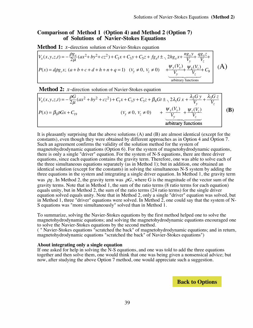
Solutions of Navier-Stokes Equations (Method 2)

39

Comparison of Method 1 (Option 4) and Method 2 (Option 7) of Solutions of Navier-Stokes Equations

Method 1: x−direction solution of Navier-Stokes equation

V x y z tg

ax by cz C x C y C z fg t hg xng yV

qg zV

P x d g x a b c d h n qVV

xx

x xx

y

x

z

y zy y

yx V V

( , , , ) ( )

( ) ; ( ) , )( )

= − + + + + + + ± + + +

= + + + + + + = ≠ ≠ + +

ρμ

ρψ ψ

2 2

1 0 0

2 2 21 3 5

( zz z

z

VV C( )

arbitrary functions

1 244 344+ 9

(A)

Method 2: x−direction solution of Navier-Stokes equation

V x y z tG

ax by cz C x C y C z Gt G xG yV

G zV

P x Gx CVV

VV

xy z

y zy y

y

z z

zV V

( , , , ) ( )

, )) )

= − + + + + + + ± + +

= + ≠ ≠ + +

ρμ β λ λ λ

β ρψ ψ

2 2

0 0

2 2 24

2 3

1

1 3 5 1

19

( ) ( (

(

arbitrary functionsarbitrary functions

1 2444 3444

(B)

It is pleasantly surprising that the above solutions (A) and (B) are almost identical (except for theconstants), even though they were obtained by different approaches as in Option 4 and Option 7.Such an agreement confirms the validity of the solution method for the system ofmagnetohydrodynamic equations (Option 6). For the system of magnetohydrodynamic equations,there is only a single "driver" equation. For the system of N-S equations, there are three driverequations, since each equation contains the gravity term. Therefore, one was able to solve each ofthe three simultaneous equations separately (as in Method 1); but in addition, one obtained anidentical solution (except for the constants) in solving the simultaneous N-S system by adding thethree equations in the system and integrating a single driver equation. In Method 1, the gravity termwas ρg . In Method 2, the gravity term was ρG, where G is the magnitude of the vector sum of thegravity terms. Note that in Method 1, the sum of the ratio terms (8 ratio terms for each equation)equals unity, but in Method 2, the sum of the ratio terms (24 ratio terms) for the single driverequation solved equals unity. Note that in Method 2, only a single "driver" equation was solved, butin Method 1, three "driver" equations were solved. In Method 2, one could say that the system of N-S equations was "more simultaneously" solved than in Method 1.

To summarize, solving the Navier-Stokes equations by the first method helped one to solve themagnetohydrodynamic equations; and solving the magnetohydrodynamic equations encouraged oneto solve the Navier-Stokes equations by the second method.( " Navier-Stokes equations "scratched the back" of magnetohydrodynamic equations; and in return,magnetohydrodynamic equations "scratched the back" of Navier-Stokes equations")

About integrating only a single equationIf one asked for help in solving the N-S equations, and one was told to add the three equationstogether and then solve them, one would think that one was being given a nonsensical advice; butnow, after studying the above Option 7 method, one would appreciate such a suggestion.

Back to Options

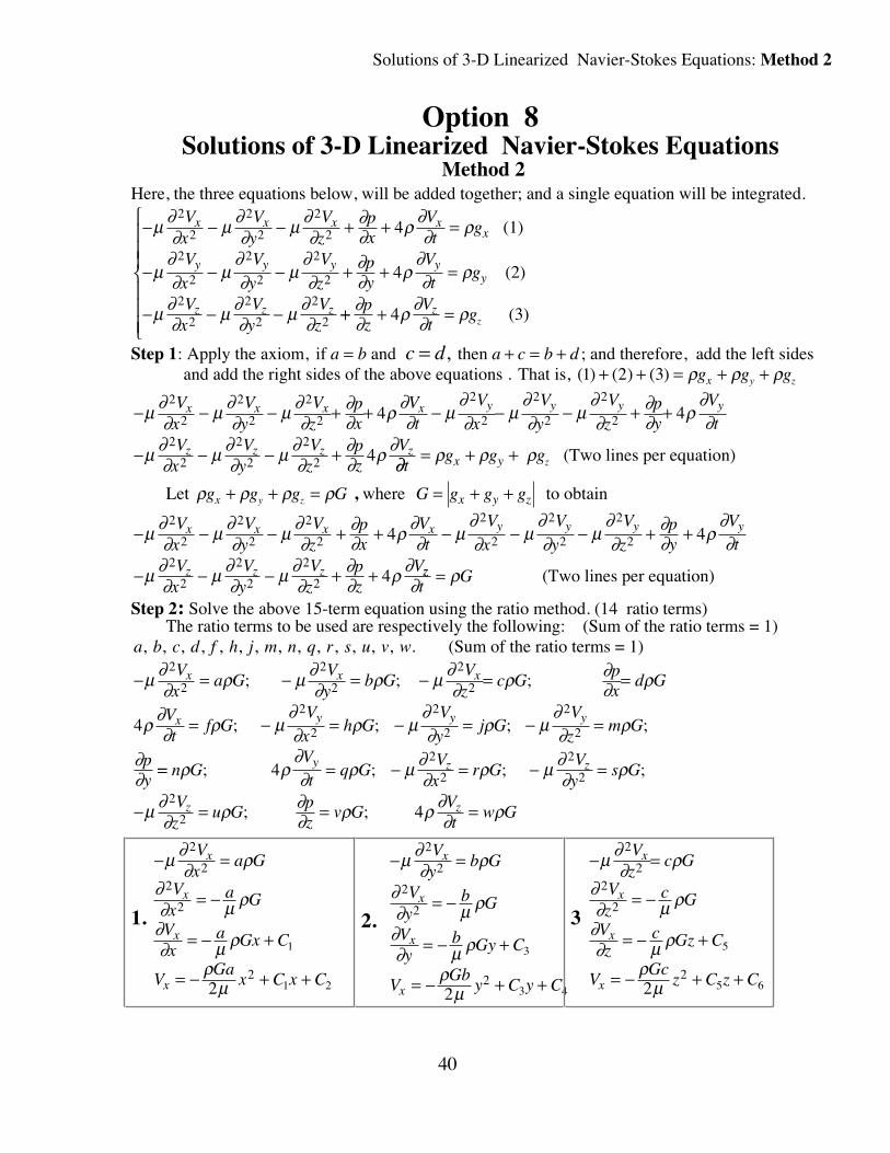
Solutions of 3-D Linearized Navier-Stokes Equations: Method 2

40

Option 8Solutions of 3-D Linearized Navier-Stokes Equations

Method 2Here, the three equations below, will be added together; and a single equation will be integrated.

− − − + + =

− − − + + =

− − −

µ ∂∂ µ ∂

∂ µ ∂∂

∂∂ ρ ∂

∂ ρ

µ∂∂ µ

∂∂ µ

∂∂

∂∂ ρ

∂∂ ρ

µ ∂∂ µ ∂

∂ µ ∂∂

2

2

2

2

2

2

2

2

2

2

2

2

2

2

2

2

2

2

4

4

Vx

Vy

Vz

px

Vt

g

Vx

Vy

Vz

py

Vt

g

Vx

Vy

Vz

x x x xx

y y y yy

z z z

(1)

(2)

++ + =

∂∂ ρ ∂

∂ ρpz

Vt

gzz4 (3)

Step 1: Apply the axiom, if and a b= c d a c b d= + = +, then ; and therefore, add the left sides and add the right sides of the above equations . That is, ( ) ( ) ( )1 2 3+ + = + +ρ ρ ρg g gx y z

− − − + + − − − + +

− − − +

µ ∂∂ µ ∂

∂ µ ∂∂

∂∂ ρ ∂

∂ µ∂∂ µ

∂∂ µ

∂∂

∂∂ ρ

∂∂

µ ∂∂ µ ∂

∂ µ ∂∂

∂∂ ρ ∂

2

2

2

2

2

2

2

2

2

2

2

2

2

2

2

2

2

2

4 4

4

Vx

Vy

Vz

px

Vt

Vx

Vy

Vz

py

Vt

Vx

Vy

Vz

pz

V

x x x x y y y y

z z z z∂∂ ρ ρ ρt

g g gx y z= + + (Two lines per equation)

Let ρ ρ ρ ρg g g Gx y z+ + = , where G g g gx y z= + + to obtain

− − − + + − − − + +

− − − + +

µ ∂∂ µ ∂

∂ µ ∂∂

∂∂ ρ ∂

∂ µ∂∂ µ

∂∂ µ

∂∂

∂∂ ρ

∂∂

µ ∂∂ µ ∂

∂ µ ∂∂

∂∂ ρ ∂

2

2

2

2

2

2

2

2

2

2

2

2

2

2

2

2

2

2

4 4

4

Vx

Vy

Vz

px

Vt

Vx

Vy

Vz

py

Vt

Vx

Vy

Vz

pz

V

x x x x y y y y

z z z zzt

G∂ ρ= (Two lines per equation)

Step 2: Solve the above 15-term equation using the ratio method. (14 ratio terms) The ratio terms to be used are respectively the following: (Sum of the ratio terms = 1)a b c d f h j m n q r s u v w, , , , , , , , , , , , , , . (Sum of the ratio terms = 1)

− = − = − = =

= − = − = − =

µ ∂∂ ρ µ ∂

∂ ρ µ ∂∂ ρ ∂

∂ ρ

ρ ∂∂ ρ µ

∂∂ ρ µ

∂∂ ρ µ

∂∂ ρ

∂∂

2

2

2

2

2

2

2

2

2

2

2

24

Vx

a GVy

b GVz

c Gpx

d G

Vt

f GVx

h GVy

j GVz

m G

py

x x x

x y y y

; ; ;

; ; ; ;

== = − = − =

− = = =

n GVt

q GV

xr G

Vy

s G

Vz

u Gpz

v GVt

w G

y z z

z z

ρ ρ∂∂ ρ µ ∂

∂ ρ µ ∂∂ ρ

µ ∂∂ ρ ∂

∂ ρ ρ ∂∂ ρ

;

4

4

2

2

2

2

2

2

; ; ;

; ;

1.

− =

= −

= − +

= − + +

µ ∂∂ ρ

∂∂ µ ρ

∂∂ µ ρ

ρµ

2

22

2

2

1

1 22

Vx

a G

Vx

a G

Vx

a Gx C

VGa

x C x C

x

x

x

x

2.

− =

= −

= − +

= − + +

µ ∂∂ ρ

∂∂ µ ρ

∂∂ µ ρ

ρµ

2

2

2

2

2

3

3 42

Vy

b G

Vy

b G

Vy

b Gy C

VGb

y C y C

x

x

x

x

3

− =

= −

= − +

= − + +

µ ∂∂ ρ

∂∂ µ ρ

∂∂ µ ρ

ρµ

2

22

2

2

5

5 62

Vz

c G

Vz

c G

Vz

c Gz C

VGc

z C z C

x

x

x

x

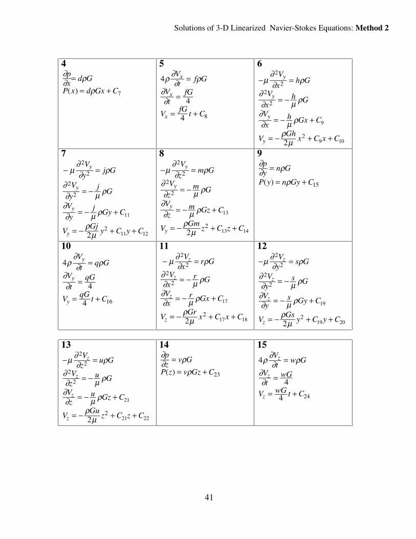
Solutions of 3-D Linearized Navier-Stokes Equations: Method 2

41

4∂∂ ρ

ρ

px

d G

P x d Gx C

== +( ) 7

5

4

4

4 8

ρ ∂∂ ρ

∂∂

Vt

f G

Vt

fG

VfG

t C

x

x

x

=

=

= +

6

− =

= −

= − +

= − + +

μ∂∂ ρ

∂∂ μ ρ

∂∂ μ ρ

ρμ

2

22

2

2

9

9 102

Vx

h G

Vx

h G

Vx

h Gx C

VGh

x C x C

y

y

y

y

7

− =

= −

= − +

= − + +

μ∂∂ ρ

∂∂ μ ρ

∂∂ μ ρ

ρμ

2

2

2

2

2

11

11 122

Vy

j G

Vy

jG

Vy

jGy C

VGj

y C y C

y

y

y

y

8

− =

= −

= − +

= − + +

μ∂∂ ρ

∂∂ μ ρ

∂∂ μ ρ

ρμ

2

22

2

2

13

13 142

Vz

m G

Vz

m G

Vz

m Gz C

VGm

z C z C

y

y

y

y

9∂∂ ρ

ρ

py

n G

P y n Gy C

=

= +( ) 15

10

4

4

4 16

ρ∂∂ ρ

∂∂

Vt

q G

Vt

qG

VqG

t C

y

y

y

=

=

= +

11

− =

= −

= − +

= − + +

μ ∂∂ ρ

∂∂ μ ρ

∂∂ μ ρ

ρμ

2

22

2

2

17

17 182

Vx

r G

Vx

r G

Vx

r Gx C

VGr

x C x C

z

z

z

z

12

− =

= −

= − +

= − + +

μ ∂∂ ρ

∂∂ μ ρ

∂∂ μ ρ

ρμ

2

2

2

2

2

19

19 202

Vy

s G

Vy

s G

Vy

s Gy C

VGs

y C y C

z

z

z

z

13

− =

= −

= − +

= − + +

μ ∂∂ ρ

∂∂ μ ρ

∂∂ μ ρ

ρμ

2

22

2

2

21

21 222

Vz

u G

Vz

u G

Vz

u Gz C

VGu

z C z C

z

z

z

z

14∂∂ ρ

ρ

pz

v G

P z v Gz C

== +( ) 23

15

4

4

4 24

ρ ∂∂ ρ

∂∂

Vt

w G

Vt

wG

V wG t C

z

z

z

=

=

= +

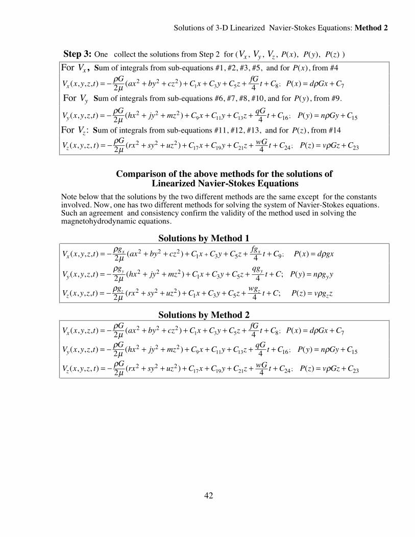
Solutions of 3-D Linearized Navier-Stokes Equations: Method 2

42

Step 3: One collect the solutions from Step 2 for (Vx , Vy , Vz , P x P y P z( ), ( ), ( ) )

For Vx , Sum of integrals from sub-equations #1, #2, #3, #5, and for P x( ), from #4

V x y z tG

ax by cz C x C y C zfG

t C P x d Gx Cx ( , , , ) ( ) ( );= − + + + + + + + = +ρµ ρ2 4

2 2 28 71 3 5

For Vy Sum of integrals from sub-equations #6, #7, #8, #10, and for P y( ), from #9.

V x y z tG

hx jy mz C x C y C zqG

t C P y n Gy Cy( , , , ) ( ) ( );= − + + + + + + + = +ρµ ρ2 4

2 2 216 159 11 13

For Vz : Sum of integrals from sub-equations #11, #12, #13, and for P z( ), from #14

V x y z tG

rx sy uz C x C y C z wG t C P z v Gz Cz ( , , , ) ( ) ( );= − + + + + + + + = +ρµ ρ2 4

2 2 224 2317 19 21

Comparison of the above methods for the solutions of Linearized Navier-Stokes Equations

Note below that the solutions by the two different methods are the same except for the constantsinvolved. Now, one has two different methods for solving the system of Navier-Stokes equations.Such an agreement and consistency confirm the validity of the method used in solving themagnetohydrodynamic equations.

Solutions by Method 1

V x y z tg

ax by cz C x C y C zfg

t C P x d gxxx x( , , , ) ( ) ( );= − + + + + + + =+

ρµ ρ2 4

2 2 21 3 5 9

V x y z tg

hx jy mz C x C y C zqg

t C P y n g yy yy y( , , , ) ( ) ; ( )= − + + + + + + + =

ρµ ρ2 4

2 2 21 3 5

V x y z tg

rx sy uz C x C y C zwg

t C P z v g zz zz z( , , , ) ( ) ; ( )= − + + + + + + + =ρµ ρ2 4

2 2 21 3 5

Solutions by Method 2

V x y z tG

ax by cz C x C y C zfG

t C P x d Gx Cx ( , , , ) ( ) ( );= − + + + + + + + = +ρµ ρ2 4

2 2 28 71 3 5

V x y z tG

hx jy mz C x C y C zqG

t C P y n Gy Cy( , , , ) ( ) ( );= − + + + + + + + = +ρµ ρ2 4

2 2 216 159 11 13

V x y z tG

rx sy uz C x C y C z wG t C P z v Gz Cz ( , , , ) ( ) ( );= − + + + + + + + = +ρµ ρ2 4

2 2 224 2317 19 21

Overall Conclusion

43

Overall ConclusionThe Navier-Stokes (N-S) equations in 3-D and 4-D have been solved analytically for the first timeby two different methods. In Method 1, the three equations were separately integrated. In Method 2, the three equations were first added together and a single equation was integrated.The solutions from these two methods were the same, except for the constants involved. The systemof magnetohydrodynamic (MHD) equations has also been solved analytically for the first time. Theexperience gained in solving the Navier-Stokes equations guided the author to solve MHDequations; and the experience from solving the MHD equations encouraged the second method ofsolving the N-S equations. The N-S solution is unique. After each term of the equation had beenmade subject of the equation to produce nine equations, and all nine equations had been integrated,only the equation with the gravity term as the subject of the equation produced the solution.The experience gained in solving the linearized equation helped the author to propose a new law,the law of definite ratio for incompressible fluid flow. This law states that in incompressible fluidflow, the other terms of the fluid flow equation divide the gravity term in a definite ratio, and eachterm utilizes gravity to function. The sum of the terms of the ratio is always unity. The applicationof this law helped speed-up the solutions of the non-linearized N-S equations as well as solutions ofthe magnetohydrodynamic equations, since there was no more experimentation as to subject of theequation. The experience from the linearized solution is that for a solution of the N-S equation, thegravity term must be the subject of the equation. It was also shown that without gravity forces on earth, there will be no incompressible fluid flowon earth as is known; and there will also be no magnetohydrodynamics.After using ratios to split the equation with the gravity term as the subject of the equation, theintegration was straightforward. The solutions and relations revealed the role of each term of theNavier-Stokes equations in fluid flow. Most importantly, the gravity term is the indispensable termin fluid flow, and it is involved in the parabolic as well as the forward motion. The pressure gradientterm is also involved in the parabolic motion. The viscosity terms are involved in parabolic, periodicand decreasingly exponential motion. As the viscosity increases, periodicity increases. The variableacceleration term is also involved in the periodic and decreasingly exponential motion. Theconvective acceleration terms produce square root function behavior and behavior of fractional termscontaining square root functions with variables in denominators and consequent turbulence behavior.From Option 1 and Option 4 results, the following statements can be made:1. The N-S equations have unique solutions.2. The N-S equations have parabolic solutions.3. The N-S equations have square root function solutions.4. The N-S equations do not have periodic solutions but have periodic relations.5.. The N-S equations do not have decreasingly exponential solutions but have decreasingly exponential relations.

Determining the ratio termsIn applications, the ratio terms a b c d f h n q, , , , , , , and others may perhaps be determined usinginformation such as initial and boundary conditions or may have to be determined experimentally.The author came to the experimental determination conclusion after referring to Example 5, page 6..The question is how did the grandmother determine the terms of the ratio for her grandchildren?Note that so far as the general solutions of the N-S equations are concerned, one needs not find thespecific values of the ratio terms.Finally, for any fluid flow design, one should always maximize the role of gravity for cost-effectiveness, durability, and dependability. Perhaps, Newton's law for fluid flow should read "Sum of everything else equals ρg" ; and this would imply the proposed new law that the otherterms divide the gravity term in a definite ratio, and each term utilizes gravity to function.

Back to Options

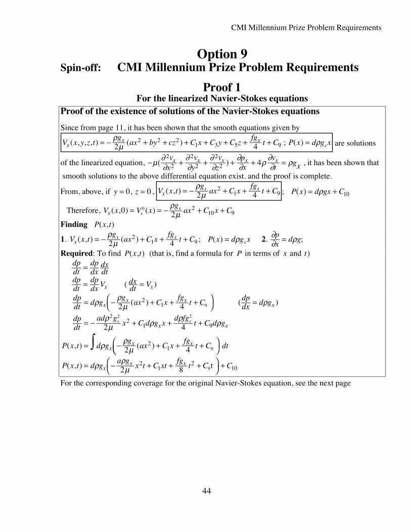
CMI Millennium Prize Problem Requirements

44

Option 9Spin-off: CMI Millennium Prize Problem Requirements

Proof 1For the linearized Navier-Stokes equations

Proof of the existence of solutions of the Navier-Stokes equations

Since from page 11, it has been shown that the smooth equations given by

V x y z tg

ax by cz C x C y C zfg

t C P x d g xxx x

x( , , , ) ( ) ( )= − + + + + + + + =ρμ ρ2 4

2 2 21 3 5 9 ; are solutions

of the linearized equation, − + + + + =μ ∂∂

∂∂

∂∂

∂∂ ρ ∂

∂ ρ( )2

2

2

2

2

2 4Vx Vx Vx x Vxx y z

px t

gx , it has been shown that

smooth solutions to the above differential equation exist. and the proof is complete.

From, above, if y z= =0 0, , V x tgax C x

fgt Cx

x x( , ) = − + + +ρμ2 4

21 9 ; P x d gx C( ) = +ρ 10

Therefore, V x V xgax C x Cx x

x( , ) ( )0 20 2

10 9= = − + +ρμ

Finding P x t( , )

1. V x tg

ax C xfg

t Cxx x( , ) ( )= − + + +ρ

μ2 42

1 9 ; P x d g xx( ) = ρ 2. ∂∂ ρpx

d g= ;

Required: To find P x t( , ) (that is, find a formula for P in terms of x and t)

dpdt

dpdx

dxdt=

dpdt

dpdx Vx= ( dxdt Vx= )

dpdt d g

gax C x

fgt C

dpdx d g

dpdt

ad gx C d g x

d fgt C d g

P x t d gg

ax C xfg

t C

xx x

x

x x

xx x

x x

= − + + +⎛⎝

⎞⎠ =

= − + + +

= − + + +⎛∫

ρ ρμ ρ

ρμ ρ ρ ρ

ρ ρμ

2 4

2 4

2 4

21

21 9

21

9

2 2

9

2

( ) )

( , ) ( )

(

⎝⎝⎞⎠

= − + + +⎛⎝

⎞⎠ +

t

dt

P x t d ga g

x t C xtfg

t C Cxx x( , ) ρ ρ

μ2 82

12

109

For the corresponding coverage for the original Navier-Stokes equation, see the next page

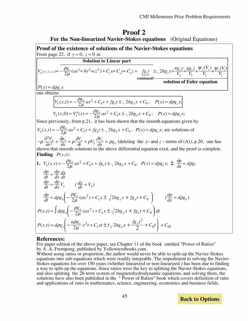
CMI Millennium Prize Problem Requirements

45

Proof 2For the Non-linearized Navier-Stokes equations (Original Equations)

Proof of the existence of solutions of the Navier-Stokes equationsFrom page 22, if y z= =0 0, in

Vg

ax by cz C x C y C z fg t hg xng yV

qg zV

VV

VVx x y z t

y z

xx x

x x y y

y

z z

z( , , , ) ( )

( ) ( )= − + + + + + + ± + + + +ρμ

ψ ψ2 22 2 2

1 3 5

continued

Solution to Linear part

solution of Euler equationl

{

6 7444444444 8444444444

1 24444444 334444444

P x d g xx( ) = ρone obtains

V x tgax C x fg t hg x C P x d g xx

xx x x( , ) ( ) ;= − + + ± + =ρ

μ ρ2 221 9 ;

V x V xgax C x hg x C P x d g xx x

xx x( , ) ( ) ( ) ;0 2 20 2

1 9= = − + ± + =ρμ ρ ;

Since previously, from p.21, it has been shown that the smooth equations given by

V x tgax C x fg t hg x C P x d g xx

xx x x( , ) ( ) ;= − + + ± + =ρ

μ ρ2 221 9 ; are solutions of

− + + + =μ ∂∂

∂∂ ρ ∂

∂ ρ ∂∂ ρ

2

2Vx

px

Vt

VVx

gx xx x

x x (deleting the y z− −and terms of (A)), p.20, one has

shown that smooth solutions to the above differential equation exist, and the proof is complete.Finding P x t( , ):

1. V x tgax C x fg t hg x C P x d g xx

xx x x( , ) ( ) ;= − + + ± + =ρ

μ ρ2 221 9; 2.

∂∂ ρpx

d g= ;

dpdt

dpdx

dxdt=

dpdt

dpdx Vx= ( dxdt Vx= )

dpdt d g

gax C x hg x fg t C

dpdx d gx

xx x x= +⎛

⎝⎜⎞⎠⎟

=− ± + +ρρ

μ ρ2 221 9( ) ) (

P x t d gg

ax C x hg x fg t C dt

P x t d ga g

x t C xt hg xfg t

C C

xx

x x

xx

xxt t

( , ) ( )

( , )

= +⎛⎝⎜

⎞⎠⎟

= +⎛

⎝⎜⎞

⎠⎟+

∫ − ± + +

− ± + +

ρρ

μ

ρρ

μ

2 2

2 2

21 9

21

2

9 102

References:For paper edition of the above paper, see Chapter 11 of the book entitled "Power of Ratios"by A. A. Frempong, published by Yellowtextbooks.com.Without using ratios or proportion, the author would never be able to split-up the Navier-Stokesequations into sub-equations which were readily integrable. The impediment to solving the Navier-Stokes equations for over 150 years (whether linearized or non-linearized ) has been due to findinga way to split-up the equations. Since ratios were the key to splitting the Navier-Stokes equations,and also splitting the 28-term system of magnetohydrodynamic equations, and solving them, thesolutions have also been published in the " Power of Ratios" book which covers definition of ratioand applications of ratio in mathematics, science, engineering, economics and business fields.

Back to Options