Embed Size (px)
Citation preview
Solving Dynamics Problems in Mathcad
Brian D. Harper
Mechanical Engineering The Ohio State University
A supplement to accompany Engineering Mechanics: Dynamics, 6th Edition
by J.L. Meriam and L.G. Kraige
JOHN WILEY & SONS, INC. New York • Chichester • Brisbane • Toronto • Singapore

CONTENTS Introduction 5 Chapter 1 An Introduction to Mathcad 7 Numerical Calculations 7 Variables and Functions 9 Graphics 11 Symbolic Math 17 Vector Algebra 20 Differentiation and Integration 23 Solving Equations 26 Chapter 2 Kinematics of Particles 33 2.1 Sample Problem 2/4 (Rectilinear Motion) 34 2.2 Problem 2/87 (Rectangular Coordinates) 37 2.3 Problem 2/120 (n-t Coordinates) 42 2.4 Sample Problem 2/9 (Polar Coordinates) 44 2.5 Sample Problem 2/10 (Polar Coordinates) 48 2.6 Problem 2/183 (Space Curvilinear Motion) 51 2.7 Sample Problem 2/16 (Constrained Motion of Connected Particles) 54 Chapter 3 Kinetics of Particles 57 3.1 Sample Problem 3/3 (Rectilinear Motion) 58 3.2 Problem 3/98 (Curvilinear Motion) 61 3.3 Sample Problem 3/17 (Potential Energy) 64 3.4 Problem 3/218 (Linear Impulse/Momentum) 66 3.5 Problem 3/250 (Angular Impulse/Momentum) 68 3.6 Problem 3/365 (Curvilinear Motion) 70
4 CONTENTS
Chapter 4 Kinetics of Systems of Particles 73 4.1 Problem 4/26 (Conservation of Momentum) 74 4.2 Problem 4/62 (Steady Mass Flow) 77 4.3 Problem 4/86 (Variable Mass) 79 Chapter 5 Plane Kinematics of Rigid Bodies 83 5.1 Problem 5/3 (Rotation) 84 5.2 Problem 5/44 (Absolute Motion) 89 5.3 Sample Problem 5/9 (Relative Velocity) 92 5.4 Problem 5/108 (Instantaneous Center) 95 5.5 Problem 5/123 (Relative Acceleration) 97 5.6 Sample Problem 5/15 (Absolute Motion) 99 Chapter 6 Plane Kinetics of Rigid Bodies 105 6.1 Sample Problem 6/2 (Translation) 106 6.2 Sample Problem 6/4 (Fixed-Axis Rotation) 112 6.3 Problem 6/98 (General Plane Motion) 114 6.4 Problem 6/104 (General Plane Motion) 117 6.5 Sample Problem 6/10 (Work and Energy) 119 6.6 Problem 6/206 (Impulse/Momentum) 124 Chapter 7 Introduction to Three-Dimensional
Dynamics of Rigid Bodies 127 7.1 Sample Problem 7/3 (General Motion) 128 7.2 Sample Problem 7/6 (Kinetic Energy) 131 Chapter 8 Vibration and Time Response 135 8.1 Sample Problem 8/2 (Free Vibration of Particles) 136 8.2 Problem 8/139 (Damped Free Vibrations) 138 8.3 Sample Problem 8/6 (Forced Vibration of Particles) 141
INTRODUCTION Computers and software have had a tremendous impact upon engineering education over the past several years and most engineering schools now incorporate computational software such as Mathcad in their curriculum. Since you have this supplement the chances are pretty good that you are already aware of this and will have to learn to use Mathcad as part of a Dynamics course. The purpose of this supplement is to help you do just that. There seems to be some disagreement among engineering educators regarding how computers should be used in an engineering course such as Dynamics. I will use this as an opportunity to give my own philosophy along with a little advice. In trying to master the fundamentals of Dynamics there is no substitute for hard work. The old fashioned taking of pencil to paper, drawing free body and mass acceleration diagrams, struggling with equations of motion and kinematic relations, etc. is still essential to grasping the fundamentals of Dynamics. A sophisticated computational program is not going to help you to understand the fundamentals. For this reason, my advice is to use the computer only when required to do so. Most of your homework can and should be done without a computer. A possible exception might be using Mathcads symbolic algebra capabilities to check some messy calculations. The problems in this booklet are based upon problems taken from your text. The problems are slightly modified since most of the problems in your book do not require a computer for the reasons discussed in the last paragraph. One of the most important uses of the computer in studying Mechanics is the convenience and relative simplicity of conducting parametric studies. A parametric study seeks to understand the effect of one or more variables (parameters) upon a general solution. This is in contrast to a typical homework problem where you generally want to find one solution to a problem under some specified conditions. For example, in a typical homework problem you might be asked something about the trajectory of a particle launched at an angle of 30 degrees from the horizontal with an initial speed of 30 ft/sec. In a parametric study of the same problem you might typically find the trajectory as a function of two parameters, the launch angle θ and initial speed v. You might then be asked to plot the trajectory for different launch angles and speeds. A plot of this type is very beneficial in visualizing the general solution to a problem over a broad range of variables as opposed to a single case.
6 INTRODUCTION
As you will see, it is not uncommon to find Mechanics problems that yield equations that cannot be solved exactly. These problems require a numerical approach that is greatly simplified by computational software such as Mathcad. Although numerical solutions are extremely easy to obtain in Mathcad this is still the method of last resort. Chapter 1 will illustrate several methods for obtaining symbolic (exact) solutions to problems. These methods should always be tried first. Only when these fail should you generate a numerical approximation. Many students encounter some difficulties the first time they try to use a computer as an aid to solving a problem. In many cases they are expecting that they have to do something fundamentally different. It is very important to understand that there is no fundamental difference in the way that you would formulate computer problems as opposed to a regular homework problem. Each problem in this booklet has a problem formulation section prior to the solution. As you work through the problems be sure to note that there is nothing peculiar about the way the problems are formulated. You will see free-body and mass acceleration diagrams, kinematic equations etc. just like you would normally write. The main difference is that most of the problems will be parametric studies as discussed above. In a parametric study you will have at least one and possibly more parameters or variables that are left undefined during the formulation. For example, you might have a general angle θ as opposed to a specific angle of 20°. If it helps, you can pretend that the variable is some specific number while you are formulating a problem. This supplement has eight chapters. The first chapter contains a brief introduction to Mathcad. If you already have some familiarity with Mathcad you can skip this chapter. Although the first chapter is relatively brief it does introduce all the methods that will be used later in the book and assumes no prior knowledge of Mathcad. Chapters 2 through 8 contain computer problems taken from chapters 2 through 8 of your textbook. Thus, if you would like to see some computer problems involving the kinetics of particles you can look at the problems in chapter 3 of this supplement. Each chapter will have a short introduction that summarizes the types of problems and computational methods used. This would be the ideal place to look if you are interested in finding examples of how to use specific functions, operations etc. This supplement uses Mathcad 13. Mathcad is a registered trademark of MathSoft, Inc., 101 Main Street, Cambridge, Massachusetts, 02142.
AN INTRODUCTION TO MATHCAD This chapter provides an introduction to the Mathcad programming language. Although the chapter is introductory in nature it will cover everything needed to solve the computer problems in this booklet. 1.1 Numerical Calculations Mathcad has four different equals signs. The most important of these are the evaluation equals sign (=) and the assignment equals sign (:=). Numerical calculations use the evaluation equals sign. As a simple example, type the following expression into a Mathcad worksheet: "(2+6^3)*4/5=". After pressing the "=" key, Mathcad will immediately evaluate the expression. It should look like the following.
2 63+( ) 45
⋅ 174.4=
Note that the result looks very much like what you would write on a sheet of paper. Now try typing "10+12/3-6*2^4=" into the worksheet. You should get the following.
10 12
3 6 24⋅−+ 9.871=
At first it may surprising that the 6*2^4 remains in the denominator. Now try entering the same keystrokes but press the space bar immediately after typing "3". Note how the blue placeholder changes when the space bar is pressed. With a little practice, you shouldn't have too much trouble getting the expression you want. The main thing is to pay attention to the placeholder. The arrow keys can also be used to move the placeholder. Numerical calculations can also include standard functions. The most commonly used functions can be found in the calculator toolbar. The calculator toolbar can be opened with View...Toolbars or by pressing shortcut button that looks like a calculator. Mathcad has many built in functions besides those shown in the
1
8 CH. 1 AN INTRODUCTION TO MATHCAD
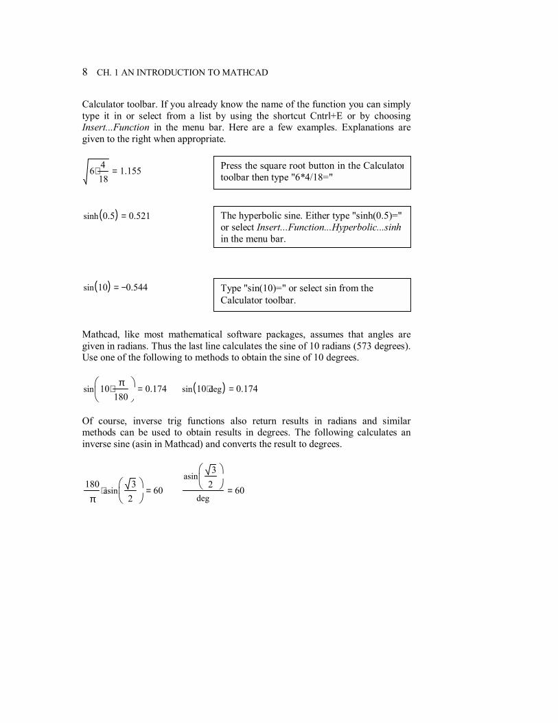
Calculator toolbar. If you already know the name of the function you can simply type it in or select from a list by using the shortcut Cntrl+E or by choosing Insert...Function in the menu bar. Here are a few examples. Explanations are given to the right when appropriate.
6 418
⋅ 1.155=
sinh 0.5( ) 0.521= sin 10( ) 0.544−= Mathcad, like most mathematical software packages, assumes that angles are given in radians. Thus the last line calculates the sine of 10 radians (573 degrees). Use one of the following to methods to obtain the sine of 10 degrees.
sin 10 π180
⋅
0.174= sin 10 deg⋅( ) 0.174=
Of course, inverse trig functions also return results in radians and similar methods can be used to obtain results in degrees. The following calculates an inverse sine (asin in Mathcad) and converts the result to degrees.
180π
asin3
2
⋅ 60= asin
32
deg60=
Press the square root button in the Calculatortoolbar then type "6*4/18="
Type "sin(10)=" or select sin from the Calculator toolbar.
The hyperbolic sine. Either type "sinh(0.5)=" or select Insert...Function...Hyperbolic...sinh in the menu bar.
INTRODUCTION TO MATHCAD 9
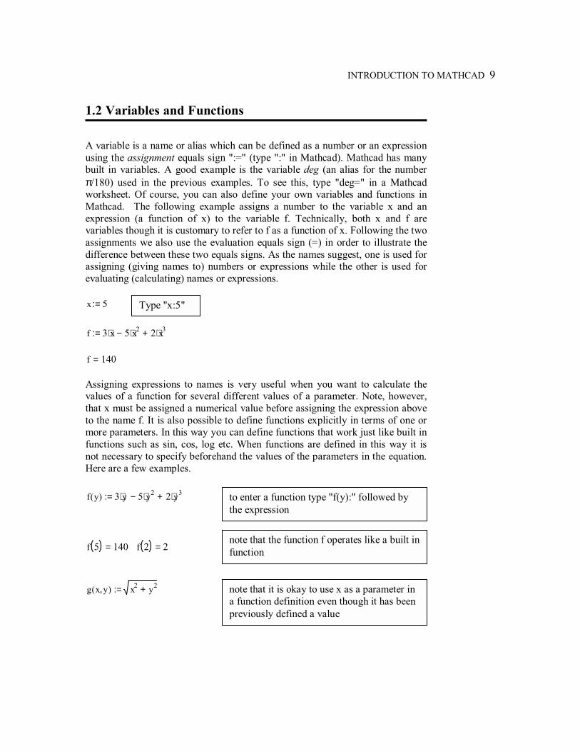
1.2 Variables and Functions A variable is a name or alias which can be defined as a number or an expression using the assignment equals sign ":=" (type ":" in Mathcad). Mathcad has many built in variables. A good example is the variable deg (an alias for the number π/180) used in the previous examples. To see this, type "deg=" in a Mathcad worksheet. Of course, you can also define your own variables and functions in Mathcad. The following example assigns a number to the variable x and an expression (a function of x) to the variable f. Technically, both x and f are variables though it is customary to refer to f as a function of x. Following the two assignments we also use the evaluation equals sign (=) in order to illustrate the difference between these two equals signs. As the names suggest, one is used for assigning (giving names to) numbers or expressions while the other is used for evaluating (calculating) names or expressions. x 5:= f 3 x⋅ 5 x2⋅− 2 x3⋅+:= f 140= Assigning expressions to names is very useful when you want to calculate the values of a function for several different values of a parameter. Note, however, that x must be assigned a numerical value before assigning the expression above to the name f. It is also possible to define functions explicitly in terms of one or more parameters. In this way you can define functions that work just like built in functions such as sin, cos, log etc. When functions are defined in this way it is not necessary to specify beforehand the values of the parameters in the equation. Here are a few examples. f y( ) 3 y⋅ 5 y2⋅− 2 y3⋅+:= f 5( ) 140= f 2( ) 2=
g x y,( ) x2 y2+:=
Type "x:5"
to enter a function type "f(y):" followed by the expression
note that the function f operates like a built in function
note that it is okay to use x as a parameter in a function definition even though it has been previously defined a value
10 CH. 1 AN INTRODUCTION TO MATHCAD
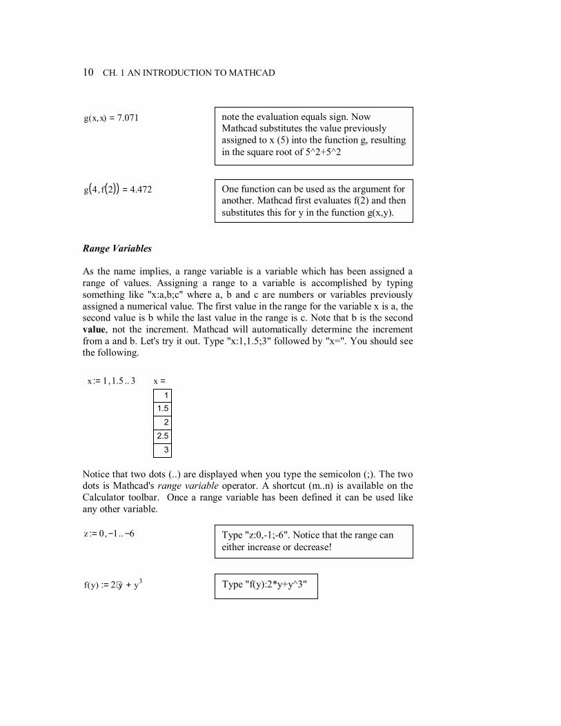
g x x,( ) 7.071= g 4 f 2( ),( ) 4.472= Range Variables As the name implies, a range variable is a variable which has been assigned a range of values. Assigning a range to a variable is accomplished by typing something like "x:a,b;c" where a, b and c are numbers or variables previously assigned a numerical value. The first value in the range for the variable x is a, the second value is b while the last value in the range is c. Note that b is the second value, not the increment. Mathcad will automatically determine the increment from a and b. Let's try it out. Type "x:1,1.5;3" followed by "x=". You should see the following.
x 1 1.5, 3..:= x1
1.5
22.5
3
=
Notice that two dots (..) are displayed when you type the semicolon (;). The two dots is Mathcad's range variable operator. A shortcut (m..n) is available on the Calculator toolbar. Once a range variable has been defined it can be used like any other variable. z 0 1−, 6−..:= f y( ) 2 y⋅ y3+:=
note the evaluation equals sign. Now Mathcad substitutes the value previously assigned to x (5) into the function g, resulting in the square root of 5^2+5^2
One function can be used as the argument for another. Mathcad first evaluates f(2) and then substitutes this for y in the function g(x,y).
Type "z:0,-1;-6". Notice that the range can either increase or decrease!
Type "f(y):2*y+y^3"
INTRODUCTION TO MATHCAD 11
f 3( ) 33=
f z( )0
-3
-12-33
-72-135
-228
=
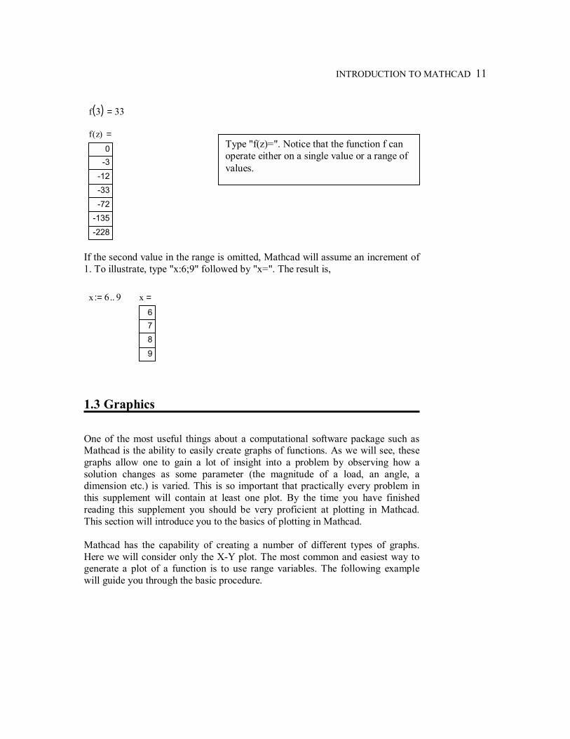
If the second value in the range is omitted, Mathcad will assume an increment of 1. To illustrate, type "x:6;9" followed by "x=". The result is,
x 6 9..:= x678
9
=
1.3 Graphics One of the most useful things about a computational software package such as Mathcad is the ability to easily create graphs of functions. As we will see, these graphs allow one to gain a lot of insight into a problem by observing how a solution changes as some parameter (the magnitude of a load, an angle, a dimension etc.) is varied. This is so important that practically every problem in this supplement will contain at least one plot. By the time you have finished reading this supplement you should be very proficient at plotting in Mathcad. This section will introduce you to the basics of plotting in Mathcad. Mathcad has the capability of creating a number of different types of graphs. Here we will consider only the X-Y plot. The most common and easiest way to generate a plot of a function is to use range variables. The following example will guide you through the basic procedure.
Type "f(z)=". Notice that the function f can operate either on a single value or a range of values.
12 CH. 1 AN INTRODUCTION TO MATHCAD
First define the function to be plotted. Type "f(x):x*exp(-x^2)" f x( ) x exp x2−( )⋅:= Now define a range variable covering the range over which you would like to plot the function. x 3− 2.9−, 3..:= Now click at the desired location on the worksheet and insert an X-Y plot by (a) selecting Insert...Graph...X-YPlot from the main menu, (b) using the shortcut key "@" or (c) selecting the X-Y Plot icon from the graph toolbar. You should see an empty graph like the following.
You should see two empty placeholders on the x and y axes. By default, the insertion point should already be on the x placeholder. If not, click on that placeholder and type "x". Now click on the y placeholder and type "f(x)". After clicking away you should see the following graph.
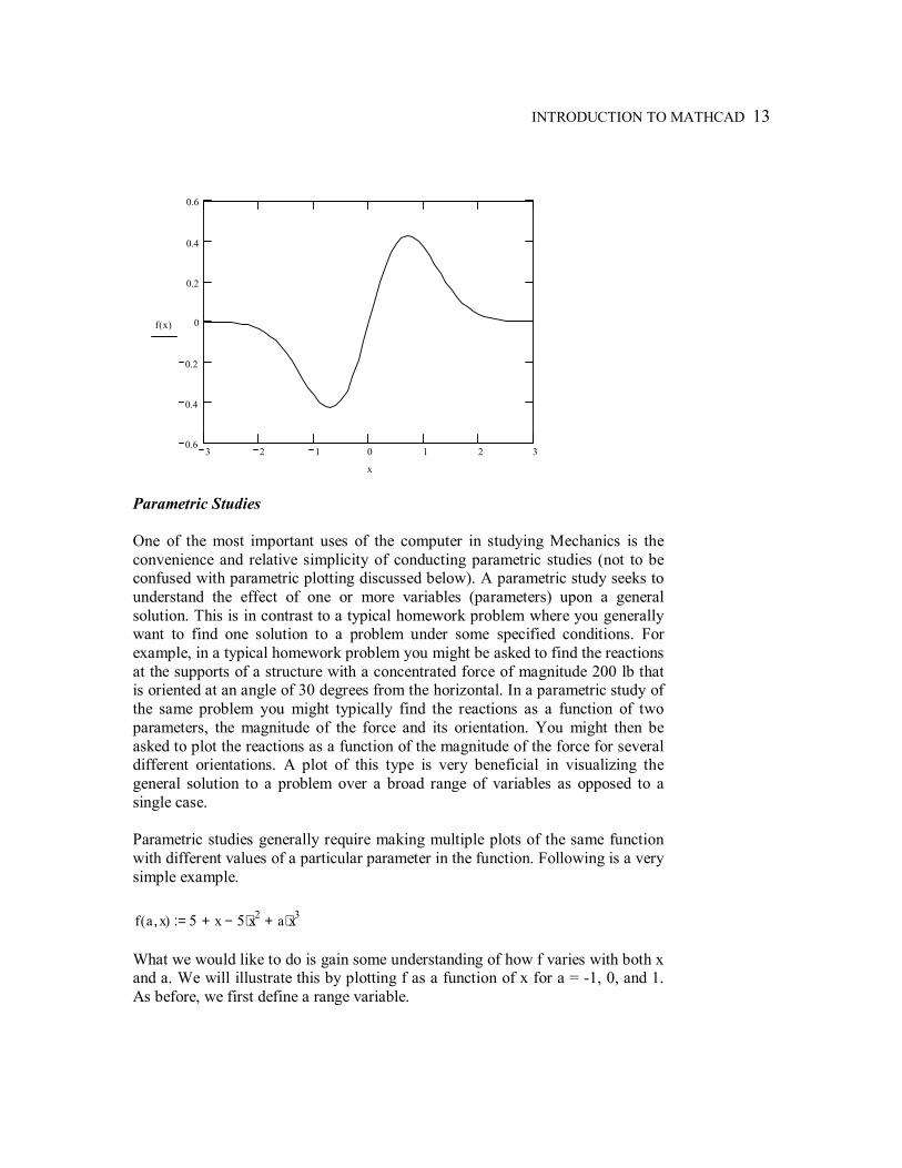
INTRODUCTION TO MATHCAD 13
3 2 1 0 1 2 30.6
0.4
0.2
0
0.2
0.4
0.6
f x( )
x
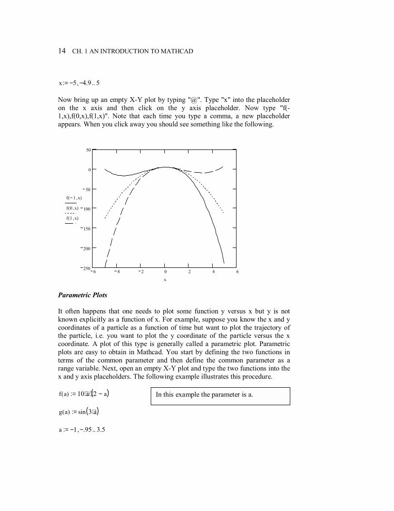
Parametric Studies One of the most important uses of the computer in studying Mechanics is the convenience and relative simplicity of conducting parametric studies (not to be confused with parametric plotting discussed below). A parametric study seeks to understand the effect of one or more variables (parameters) upon a general solution. This is in contrast to a typical homework problem where you generally want to find one solution to a problem under some specified conditions. For example, in a typical homework problem you might be asked to find the reactions at the supports of a structure with a concentrated force of magnitude 200 lb that is oriented at an angle of 30 degrees from the horizontal. In a parametric study of the same problem you might typically find the reactions as a function of two parameters, the magnitude of the force and its orientation. You might then be asked to plot the reactions as a function of the magnitude of the force for several different orientations. A plot of this type is very beneficial in visualizing the general solution to a problem over a broad range of variables as opposed to a single case. Parametric studies generally require making multiple plots of the same function with different values of a particular parameter in the function. Following is a very simple example. f a x,( ) 5 x+ 5 x2⋅− a x3⋅+:= What we would like to do is gain some understanding of how f varies with both x and a. We will illustrate this by plotting f as a function of x for a = -1, 0, and 1. As before, we first define a range variable.
14 CH. 1 AN INTRODUCTION TO MATHCAD
x 5− 4.9−, 5..:= Now bring up an empty X-Y plot by typing "@". Type "x" into the placeholder on the x axis and then click on the y axis placeholder. Now type "f(-1,x),f(0,x),f(1,x)". Note that each time you type a comma, a new placeholder appears. When you click away you should see something like the following.
6 4 2 0 2 4 6250
200
150
100
50
0
50
f 1− x,( )
f 0 x,( )
f 1 x,( )
x
Parametric Plots It often happens that one needs to plot some function y versus x but y is not known explicitly as a function of x. For example, suppose you know the x and y coordinates of a particle as a function of time but want to plot the trajectory of the particle, i.e. you want to plot the y coordinate of the particle versus the x coordinate. A plot of this type is generally called a parametric plot. Parametric plots are easy to obtain in Mathcad. You start by defining the two functions in terms of the common parameter and then define the common parameter as a range variable. Next, open an empty X-Y plot and type the two functions into the x and y axis placeholders. The following example illustrates this procedure. f a( ) 10 a⋅ 2 a−( )⋅:= g a( ) sin 3 a⋅( ):= a 1− .95−, 3.5..:=
In this example the parameter is a.
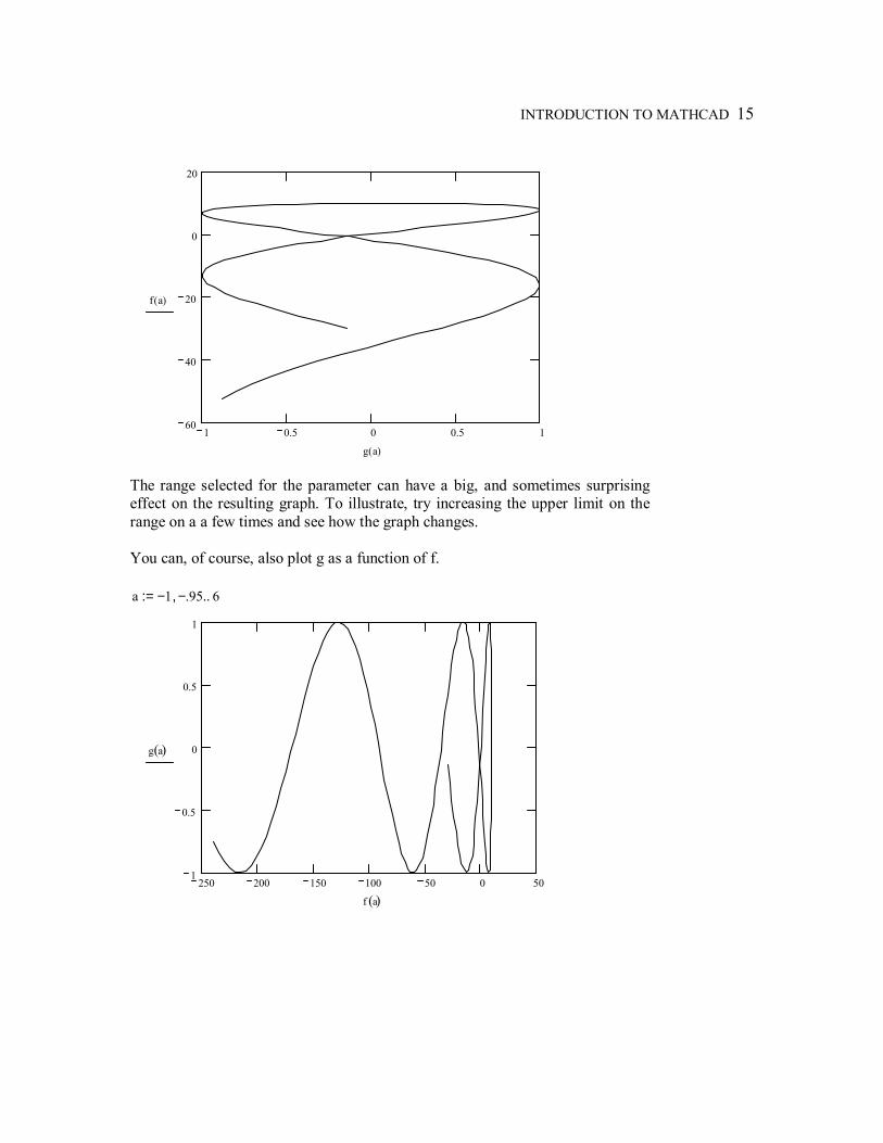
INTRODUCTION TO MATHCAD 15
1 0.5 0 0.5 160
40
20
0
20
f a( )
g a( )
The range selected for the parameter can have a big, and sometimes surprising effect on the resulting graph. To illustrate, try increasing the upper limit on the range on a a few times and see how the graph changes. You can, of course, also plot g as a function of f. a 1− .95−, 6..:=
250 200 150 100 50 0 501
0.5
0
0.5
1
g a( )
f a( )
16 CH. 1 AN INTRODUCTION TO MATHCAD
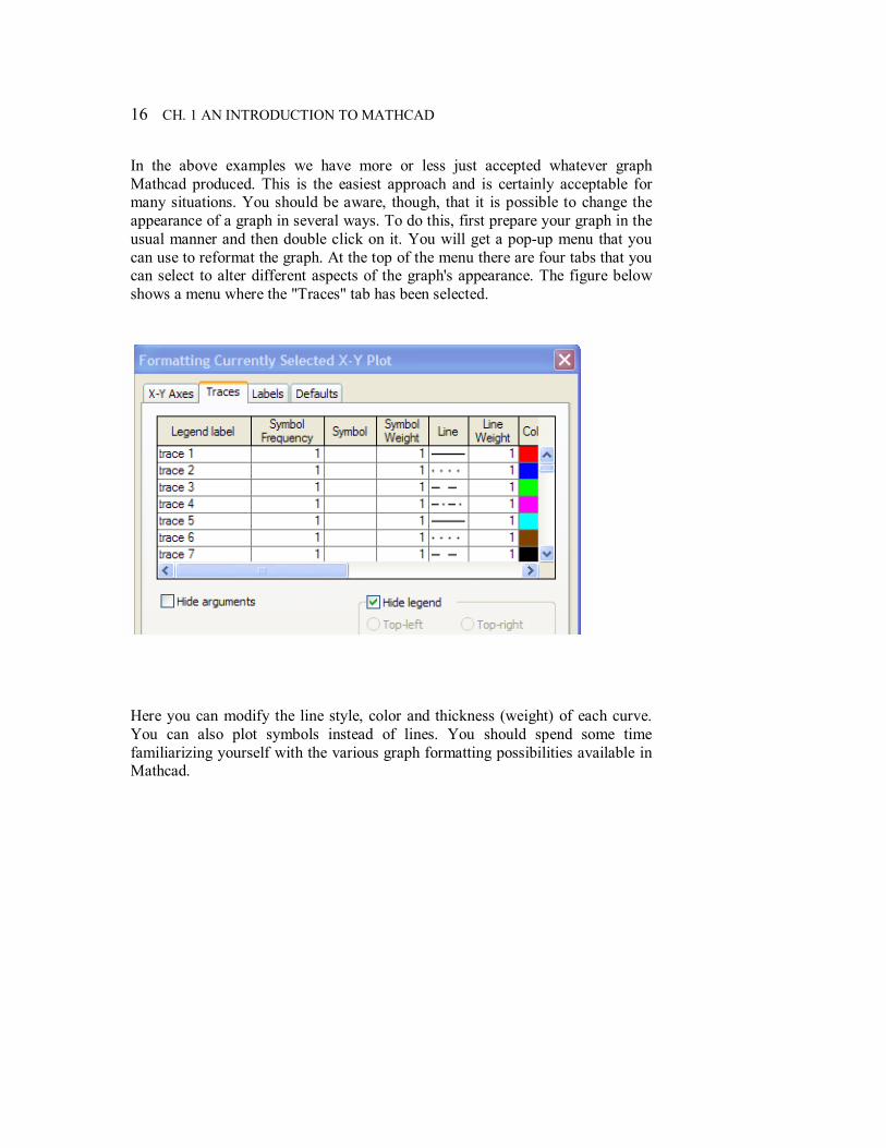
In the above examples we have more or less just accepted whatever graph Mathcad produced. This is the easiest approach and is certainly acceptable for many situations. You should be aware, though, that it is possible to change the appearance of a graph in several ways. To do this, first prepare your graph in the usual manner and then double click on it. You will get a pop-up menu that you can use to reformat the graph. At the top of the menu there are four tabs that you can select to alter different aspects of the graph's appearance. The figure below shows a menu where the "Traces" tab has been selected. Here you can modify the line style, color and thickness (weight) of each curve. You can also plot symbols instead of lines. You should spend some time familiarizing yourself with the various graph formatting possibilities available in Mathcad.
INTRODUCTION TO MATHCAD 17
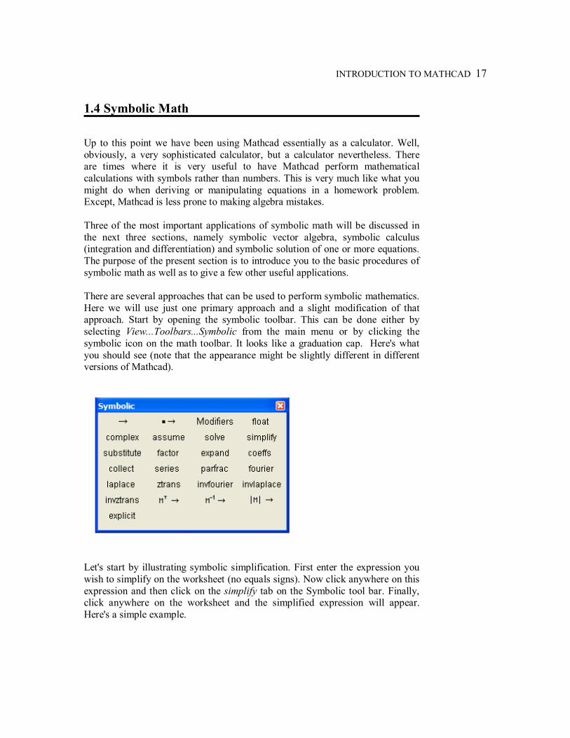
1.4 Symbolic Math Up to this point we have been using Mathcad essentially as a calculator. Well, obviously, a very sophisticated calculator, but a calculator nevertheless. There are times where it is very useful to have Mathcad perform mathematical calculations with symbols rather than numbers. This is very much like what you might do when deriving or manipulating equations in a homework problem. Except, Mathcad is less prone to making algebra mistakes. Three of the most important applications of symbolic math will be discussed in the next three sections, namely symbolic vector algebra, symbolic calculus (integration and differentiation) and symbolic solution of one or more equations. The purpose of the present section is to introduce you to the basic procedures of symbolic math as well as to give a few other useful applications. There are several approaches that can be used to perform symbolic mathematics. Here we will use just one primary approach and a slight modification of that approach. Start by opening the symbolic toolbar. This can be done either by selecting View...Toolbars...Symbolic from the main menu or by clicking the symbolic icon on the math toolbar. It looks like a graduation cap. Here's what you should see (note that the appearance might be slightly different in different versions of Mathcad). Let's start by illustrating symbolic simplification. First enter the expression you wish to simplify on the worksheet (no equals signs). Now click anywhere on this expression and then click on the simplify tab on the Symbolic tool bar. Finally, click anywhere on the worksheet and the simplified expression will appear. Here's a simple example.
18 CH. 1 AN INTRODUCTION TO MATHCAD
a x⋅ b x2⋅+( )2
x4
Here's the expression we want to simplify. If you need help, type "(a*x+b*x^2)^2[space bar]/x^4". Now click anywhere on the expression and then press the simplify tab. After clicking away you should see the following.
a x⋅ b x2⋅+( )2
x4simplify
1
x2a b x⋅+( )2⋅→
You can also simplify expressions containing previously defined functions. Here's another way to obtain the simplification above. See if you can reproduce it on your worksheet. f a b, x,( ) a x⋅ b x2⋅+:= g x( ) x4:= f a b, x,( )2
g x( )simplify
1
x2a b x⋅+( )2⋅→
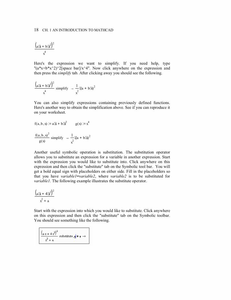
Another useful symbolic operation is substitution. The substitution operator allows you to substitute an expression for a variable in another expression. Start with the expression you would like to substitute into. Click anywhere on this expression and then click the "substitute" tab on the Symbolic tool bar. You will get a bold equal sign with placeholders on either side. Fill in the placeholders so that you have variable1=variable2, where variable2 is to be substituted for variable1. The following example illustrates the substitute operator.
a x⋅ 4 x2⋅+( )2
x2 a+
Start with the expression into which you would like to substitute. Click anywhere on this expression and then click the "substitute" tab on the Symbolic toolbar. You should see something like the following.
INTRODUCTION TO MATHCAD 19
Click in the left placeholder and type "a". Now click in the right placeholder and type "1+x^2". You should see the following result.
a x⋅ 4 x2⋅+( )2
x2 a+substitute a 1 x2+,
1 x2+( ) x⋅ 4 x2⋅+ 2
2 x2⋅ 1+( )→
It is also possible to substitute previously defined functions. f x( ) x2 1+:=
2 x⋅ 4 x2⋅+( )2
x2 2+substitute x f x( ),
2 2 x2⋅+ 4 1 x2+( )2⋅+
2
1 x2+( )22+
→
The results following a substitution are often rather messy. To simplify, one could always copy the final result into the clipboard, paste it onto the worksheet, and then follow the procedure above to simplify. It is also possible to do several symbolic operations at once. The following example shows a substitution followed by a simplification. The procedure is the same as for substitution with one difference. After filling out the before and after placeholders, click on the "simplify" tab before clicking away.
2 x⋅ 4 x2⋅+( )2
x2 2+
substitute x f x( ),
simplify4 3 5 x2⋅+ 2 x4⋅+( )2
3 2 x2⋅+ x4+( )⋅→
Finally, here is an example with two substitutions followed by simplification.
a x⋅ b x2⋅+( )2
x5
substitute a x3 tan x( )+,
substitute b x2−,
simplify
1
x3tan x( )2⋅→
20 CH. 1 AN INTRODUCTION TO MATHCAD
1.5 Vector Algebra The main application of vector algebra is in three dimensional problems where the geometry is difficult to visualize. Some of these difficulties include finding the x, y, and z components of a vector, moment arms for a force, projections of a force onto a line etc. The most useful vector operations are finding the magnitude of a vector and finding the dot or cross product of two vectors. First we need to learn how to represent a vector in Mathcad. Start by opening the Vector and Matrix Toolbar. You can do this by selecting View...Toolbars...Matrix or by clicking the matrix icon on the Math Toolbar (it looks like a 3x3 matrix). Cartesian vectors are represented by three element column matrices. The following example shows how to create a vector. Start by typing "u:". Now click on the matrix icon on the Vector and Matrix Toolbar. You can also select Insert...Matrix or use the shortcut CNTRL+M. In the popup menu select 3 rows and 1 column. After clicking OK, you should see the following
u
:=
Now fill in the placeholders with the x, y, and z components of the vector. For example,
u
3
2−
6
:=
Once the vector has been defined you can refer to the components of the vectors by typing the name of the vector with an index. Indices start at 0 in Mathcad so an index of 0, 1, and 2 correspond to x, y, and z. Indices are entered by typing "[". Don't confuse an index with a subscript, which is obtained by typing ".". For example, to print the y component of u type "u[1=". u1 2−= To find the magnitude of u, select the absolute value icon (|x|) from the Vector and Matrix Toolbar. In the placeholder type "u=". You should see the following.
u 7=
INTRODUCTION TO MATHCAD 21
In Statics, we often need to find unit vectors. A unit vector in the direction of u can be obtained by dividing u by the magnitude of u.
nuu
:=
n
0.429
0.286−
0.857
=
As an example of the above, suppose that you have a force F with magnitude 100 lb and with a line of action passing from point A (2, 0, 3) toward B (7, -2, 5). We can represent F as a Cartesian vector in Mathcad as follows.
rA
2
03
:= rB
7
2−
5
:=
rAB rA rB−:=
F 100rAB
rAB⋅:=
F
87.039−
34.81634.816−
=
Dot and cross product operators can also be selected from the Vector and Matrix Toolbar. Shortcuts are * for dot product and CNTRL+8 for cross product. Here are a few examples using the vectors we have already defined above. u F⋅ 539.641−=
rA rB×
6
114−
=
M rA F×:= M
104.447−
191.485−
69.631
=
22 CH. 1 AN INTRODUCTION TO MATHCAD
Vector operations can also be carried out symbolically. You will, of course, use the symbolic equals sign → instead of the evaluation equal sign =. Here are a few examples.
u
a
b
c
:=
a v
p
34
:=
p
w
x
5−
4
:=
x
After typing in the above three vectors you probably noticed that some of the variables appear in red since they have not been defined. This would obviously create a problem if you were going to evaluate some numerical results, however, it has no effect on symbolic calculations as can be seen from the following. u v⋅ a p⋅ 3 b⋅+ 4 c⋅+→
vv
p
p( )2 25+
12
3
p( )2 25+
12
4
p( )2 25+
12
→
u v×
4 b⋅ 3 c⋅−
c p⋅ 4 a⋅−
3 a⋅ b p⋅−
→
w u v×( )⋅ 0 solve x,5− c⋅ p⋅ 32 a⋅ 4 b⋅ p⋅−+( )−
4 b⋅ 3 c⋅−( )→
INTRODUCTION TO MATHCAD 23
1.6 Differentiation and Integration Mechanics problems often require integration and/or differentiation. In Mathcad, you can perform these operations either numerically or symbolically. Before we get started you will want to open the Calculus Toolbar. You can open this by pressing the icon in the math toolbar or by selecting View...Toolbars from the main menu. The icons we will be using are those for the first and nth derivative and the definite and indefinite integral. The definite integral has a and b as integration limits. You may also want to open the Symbolic Toolbar. Let's get started with a simple example of symbolic differentiation. Start by selecting the icon for the first derivative. Here's what you should see. dd
Note that there are two placeholders. Into the placeholder on the right hand side type the expression that you would like to differentiate (for this example, type "(a*sec(b*t))"). Then click on the placeholder in the denominator and enter the variable that you would like to differentiate with respect to. You should see the following.
ta sec b t⋅( )⋅( )d
d
Now click anywhere on this expression and click on the symbolic evaluation icon (→) in the Symbolic Toolbar. After clicking away you will see the result of the symbolic differentiation.
ta sec b t⋅( )⋅( )d
da sec b t⋅( )⋅ tan b t⋅( )⋅ b⋅→
Higher order derivatives follow the same procedure except that there is an additional placeholder to fill in for the order of differentiation. See if you can reproduce the following result.
3xa ln b x+( )⋅d
d
32
a
b x+( )3⋅→
You can also use derivatives in defining functions. As an example, suppose a particle moves in a straight line and its position s is known as a function of time. From your elementary physics course you probably know that the first and second derivatives of the position give the velocity and acceleration of the particle.
24 CH. 1 AN INTRODUCTION TO MATHCAD
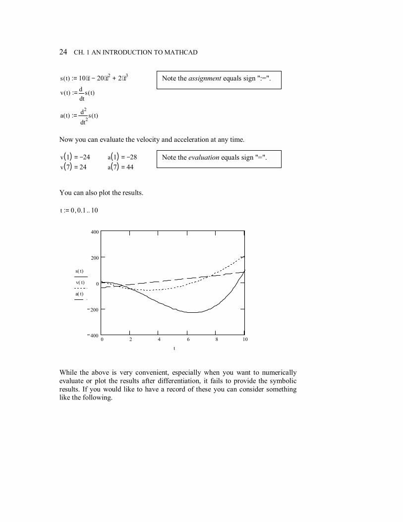
s t( ) 10 t⋅ 20 t2⋅− 2 t3⋅+:=
v t( )ts t( )d
d:=
a t( )2ts t( )d
d
2:=
Now you can evaluate the velocity and acceleration at any time. v 1( ) 24−= a 1( ) 28−= v 7( ) 24= a 7( ) 44= You can also plot the results. t 0 0.1, 10..:=
0 2 4 6 8 10400
200
0
200
400
s t( )
v t( )
a t( )
t
While the above is very convenient, especially when you want to numerically evaluate or plot the results after differentiation, it fails to provide the symbolic results. If you would like to have a record of these you can consider something like the following.
Note the assignment equals sign ":=".
Note the evaluation equals sign "=".
INTRODUCTION TO MATHCAD 25
s t( ) 10 t⋅ 20 t2⋅− 2 t3⋅+:= position
v t( )ts t( )d
d:=
velocity,
ts t( )d
d10 40 t⋅− 6 t2⋅+→
a t( )2ts t( )d
d
2:= acceleration,
2ts t( )d
d
240− 12 t⋅+→
or, tv t( )d
d40− 12 t⋅+→
The procedure for performing integrations is very similar to that for differentiation. For example, to perform a symbolic integration: (a) click on the icon for either a definite or indefinite integral (or use the shortcut key Shift+7 (or &) for definite and Cntrl+i for indefinite), (b) fill in the placeholders, (c) click anywhere on the expression and (d) click the Symbolic Evaluation icon (or use the short cut Cntrl+.). See if you can reproduce the following integrals.
xsin b x⋅( )⌠⌡
dcos b x⋅( )−
b→
c
d
xsin b x⋅( )⌠⌡
dcos d b⋅( )−
bcos c b⋅( )
b+→
xln x( )⌠⌡
d x ln x( )⋅ x−→ c
d
xln x( )⌠⌡
d d ln d( )⋅ d− c ln c( )⋅− c+→
If a definite integral contains no unknown parameters either in the integrand or the integration limits, the above procedure will provide numerical answers. Here are a few examples.
0
3
xx 3 x3⋅+( )⌠⌡
d261
4→
2
5
xln x( )⌠⌡
d 5 ln 5( )⋅ 3− 2 ln 2( )⋅−→
Note that Mathcad will try to return an exact result when the Symbolic Evaluation procedure is used. This results in fractions or functions as in the above examples. This is very useful in some situations, however, one often wants to know the numerical answer without having to evaluate a result such as the above with a calculator. Thus, Mathcad also allows you to obtain results for numerical integration as floating point numbers. This can be accomplished by following the same procedure outlined above except that for step (d) you press
26 CH. 1 AN INTRODUCTION TO MATHCAD
the equals sign "=" on your keyboard instead of clicking the Symbolic Evaluation icon. To illustrate, we will repeat the same two integrals above.
0
3
xx 3 x3⋅+( )⌠⌡
d 65.25= 2
5
xln x( )⌠⌡
d 3.661=
1.7 Solving Equations Solving a single equation symbolically can be accomplished in a manner very similar to other symbolic operations considered earlier. As an example, try typing the following equation on to your worksheet, being sure to type Cntrl = for the equals sign (you should see a bold equals sign =). a x2⋅ b x⋅+ c+ 0 Click anywhere on the equation and then click solve on the Symbolic Toolbar . Type the variable you wish to solve for (in this example x) in the placeholder and the click away. You should see the following.
a x2⋅ b x⋅+ c+ 0 solve x,
12 a⋅( ) b− b2 4 a⋅ c⋅−( )
12
+
⋅
12 a⋅( ) b− b2 4 a⋅ c⋅−( )
12
−
⋅
→
Note that Mathcad has found both solutions to the (hopefully) familiar quadratic equation. If the equals sign is omitted, Mathcad will assume that the expression is set equal to zero, i.e. Mathcad will find the roots of the expression. Here is an alternative way to obtain the above result.
a x2⋅ b x⋅+ c+ solve x,
12 a⋅( ) b− b2 4 a⋅ c⋅−( )
12
+
⋅
12 a⋅( ) b− b2 4 a⋅ c⋅−( )
12
−
⋅
→
If the variable being solved for is the only unknown in the equation, Mathcad will return a number as the result. Here are a couple of examples.
INTRODUCTION TO MATHCAD 27
2 x2⋅ 4 x⋅+ 12− solve x,1− 7+
1− 7−
→
5 sin θ( )⋅ cos θ( )− 1 solve θ,π
atan512
→
You can also solve equations using Given...Find. For the symbolic case, one starts with the basic Given...Find format shown below. Given a x2⋅ b x⋅+ c+ 0 Find(x) Now click on "Find(x)" and then click on the Symbolic Evaluation icon (→). After clicking away you should see the following result. Given a x2⋅ b x⋅+ c+ 0
Find x( )1
2 a⋅( ) b− b2 4 a⋅ c⋅−( )12
+
⋅
12 a⋅( ) b− b2 4 a⋅ c⋅−( )
12
−
⋅
→
For a numerical solution you would use the same procedure but type "Find(x)=". Here's an example. g x( ) 2 x2⋅ 1+ 10 sin x( )⋅−:= x 0:= Given g x( ) 0 Find x( ) 0.102=
28 CH. 1 AN INTRODUCTION TO MATHCAD
x 2:= Given g x( ) 0 Find x( ) 2.008= Given...Find can also be used to solve simultaneous equations either symbolically or numerically. The approach is essentially the same as that described above for a single equation except, of course, that more than one equation will appear between the Given and Find statements. Also, for numerical solutions, an initial guess should be provided for all unknowns. Following are several examples. An easy way to tell at a glance whether the solution is symbolic or numerical is to see whether the symbolic evaluation symbol (→) appears after Find. Given
P− sin β( )⋅ Bx+ Ax− 0 Ay P cos β( )⋅+ w a⋅− 0
P a⋅ cos β( )⋅ P b⋅ sin β( )⋅− Bx c⋅+12
w⋅ a2⋅− 0
Find Ax Ay, Bx,( )
12
2− P⋅ sin β( )⋅ c⋅ 2 P⋅ a⋅ cos β( )⋅− 2 P⋅ b⋅ sin β( )⋅+ w a2⋅+( )c
⋅
P− cos β( )⋅ w a⋅+
12
2− P⋅ a⋅ cos β( )⋅ 2 P⋅ b⋅ sin β( )⋅+ w a2⋅+( )c
⋅
→
Given
A subscript can be obtained by typing "."before the subscript. For example, by typing"A.x".
INTRODUCTION TO MATHCAD 29
x2 y2+ 12 x y⋅ 4
Find x y,( )5 1−
5 1+
1− 5−
1 5−
5 1+
5 1−
1 5−
1− 5−
→
Note that each column in the last result represents a solution. Thus, in the last example, Mathcad has found four solutions, the first being x = 15 − and y =
15 + . x 0:= y 0:= z 0:= Given x2 y+ 12 x y⋅ 4 x y− z
Find x y, z,( )
3.284
1.2182.065
=
x 0:= y 5:= z 5:=
Given x2 y+ 12 x y⋅ 4 x y− z
Find x y, z,( )
0.337
11.88711.55−
=
This is our initial guess for a numerical solution
Now let's try another guess for the same set of equations.
30 CH. 1 AN INTRODUCTION TO MATHCAD
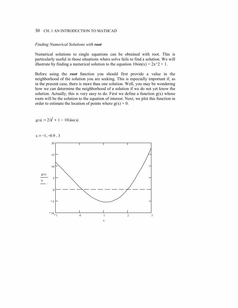
Finding Numerical Solutions with root Numerical solutions to single equations can be obtained with root. This is particularly useful in those situations where solve fails to find a solution. We will illustrate by finding a numerical solution to the equation 10sin(x) = 2x^2 + 1. Before using the root function you should first provide a value in the neighborhood of the solution you are seeking. This is especially important if, as in the present case, there is more than one solution. Well, you may be wondering how we can determine the neighborhood of a solution if we do not yet know the solution. Actually, this is very easy to do. First we define a function g(x) whose roots will be the solution to the equation of interest. Next, we plot this function in order to estimate the location of points where g(x) = 0. g x( ) 2 x2⋅ 1+ 10 sin x( )⋅−:= x 1− 0.9−, 3..:=
1 0 1 2 310
5
0
5
10
15
20
g x( )
0
x
INTRODUCTION TO MATHCAD 31
From the graph above we see that g(x) = 0 in two places, about x = 0 and x = 2. These results provide our initial guesses for the root command. Here's how it works. x 0:= root g x( ) x,( ) 0.102= x 2:= root g x( ) x,( ) 2.008= Or, equivalently, x 0:= x1 root g x( ) x,( ):= x1 0.102= x 2:= x2 root g x( ) x,( ):= x2 2.008=

KINEMATICS OF PARTICLES Kinematics involves the study of the motion of bodies irrespective of the forces that may produce that motion. Mathcad can be very useful in solving particle kinematics problems. Problem 2.1 is a rectilinear motion problem illustrating symbolic integration. The formulation of this problem results in an equation that cannot be solved exactly except with some rather sophisticated mathematics. When this occurs it is generally easiest to obtain either a graphical or numerical solution. This problem illustrates both approaches with the numerical result being obtained with GivenFind. Problem 2.2 is a rectangular coordinates problem that illustrates GivenFind as well as symbolic differentiation. Problem 2.3 is a relatively straightforward problem where Mathcad is used to generate a plot that might be useful in a parametric study. The path of a particle is depicted using a parametric plot and a polar plot in problem 2.4. In problem 2.5, the r-θ components of the velocity are determined using symbolic differentiation. The problem also illustrates how computer algebra can simplify what might normally be a rather tedious algebra problem. Symbolic differentiation is further illustrated in problems 2.6 and 2.7. Problem 2.7 is particularly interesting in that it requires differentiation with respect to time of a function whose explicit time dependence is unknown. This happens rather frequently in Dynamics so it is useful to know how to accomplish this with Mathcad.
2
34 CH. 2 KINEMATICS OF PARTICLES
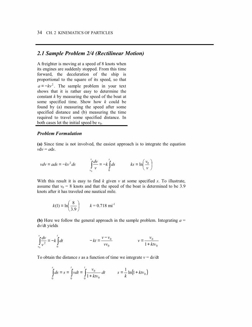
2.1 Sample Problem 2/4 (Rectilinear Motion) A freighter is moving at a speed of 8 knots when its engines are suddenly stopped. From this time forward, the deceleration of the ship is proportional to the square of its speed, so that
2kva −= . The sample problem in your text shows that it is rather easy to determine the constant k by measuring the speed of the boat at some specified time. Show how k could be found by (a) measuring the speed after some specified distance and (b) measuring the time required to travel some specified distance. In both cases let the initial speed be v0. Problem Formulation (a) Since time is not involved, the easiest approach is to integrate the equation vdv = ads.
dskvadsvdv 2−== ∫∫ −=sv
v
dskvdv
00
=
vvks 0ln
With this result it is easy to find k given v at some specified s. To illustrate, assume that v0 = 8 knots and that the speed of the boat is determined to be 3.9 knots after it has traveled one nautical mile.
=
9.38ln)1(k k = 0.718 mi-1
(b) Here we follow the general approach in the sample problem. Integrating a = dv/dt yields
∫∫ −=tv
v
dtkvdv
02
0
0
0
vvvv
kt−
=− 0
0
1 ktvv
v+
=
To obtain the distance s as a function of time we integrate v = ds/dt
∫ ∫∫ +===
t ts
dtktv
vvdtsds
0 0 0
0
0 1 ( )01ln1 ktv
ks +=
KINEMATICS OF PARTICLES 35
This equation turns out to be very difficult to solve for k. A good mathematician or someone familiar with symbolic algebra software might be able to find the general solution for k in terms of the so-called LambertW function (LambertW(x) is the solution of the equation yey = x). Even if this solution were found it would be of little use in most practical situations. For example, you would have to spend some time familiarizing yourself with the function. Once this is done you would still have to use a program like Maple or a mathematical handbook to evaluate the function. For these reasons it is probably easiest to find k either graphically or numerically. Obtaining a numerical solution with Mathcad is so easy that there is little reason not to use this approach. It is generally advisable though to use a graphical approach even when a numerical solution is being obtained. This is the best way to identify whether there are multiple solutions to the problem and also serves as a useful check on the numerical results. Thus, both approaches are illustrated in the worksheet below. The usual way to generate a graphical solution is to rearrange the equation so as to give a function that is zero at points that are solutions to the original equation. Rearranging the equation above in this manner yields, ( ) 01ln 0 =+−= ktvksf Given values of s, t, and v0, f can be plotted versus k. The value of k at which f = 0 provides the solution to the original equation. Mathcad Worksheet Although the integrations are simple in this problem, we'll go ahead and evaluate them symbolically for purposes of illustration.
s_a1−
kv0
v
x1x
⌠⌡
d⋅:=v
s_a1−
kln v( ) ln v0( )−( )⋅→
s_b
0
t
xv0
1 k v0⋅ x⋅+
⌠⌡
d:=
t
s_bln 1 t k⋅ v0⋅+( )
k→
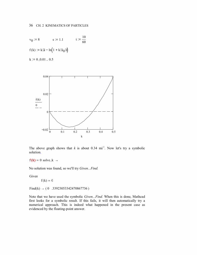
To illustrate the graphical solution, take v0 = 8 knots and assume that the boat is found to move 1.1 nautical miles after 10 minutes.
36 CH. 2 KINEMATICS OF PARTICLES
v0 8:= s 1.1:= t1060
:=
f k( ) k s⋅ ln 1 k v0⋅ t⋅+( )−:= k 0 0.01, 0.5..:=
0 0.1 0.2 0.3 0.4 0.50.02
0
0.02
0.04
f k( )
0
k
The above graph shows that k is about 0.34 mi-1. Now let's try a symbolic solution. f k( ) 0 solve k, →f k( )
No solution was found, so we'll try Given...Find. Given
f k( ) 0
Find k( ) 0 .33923053342470867736( )→ Note that we have used the symbolic Given...Find. When this is done, Mathcad first looks for a symbolic result. If this fails, it will then automatically try a numerical approach. This is indeed what happened in the present case as evidenced by the floating-point answer.
KINEMATICS OF PARTICLES 37
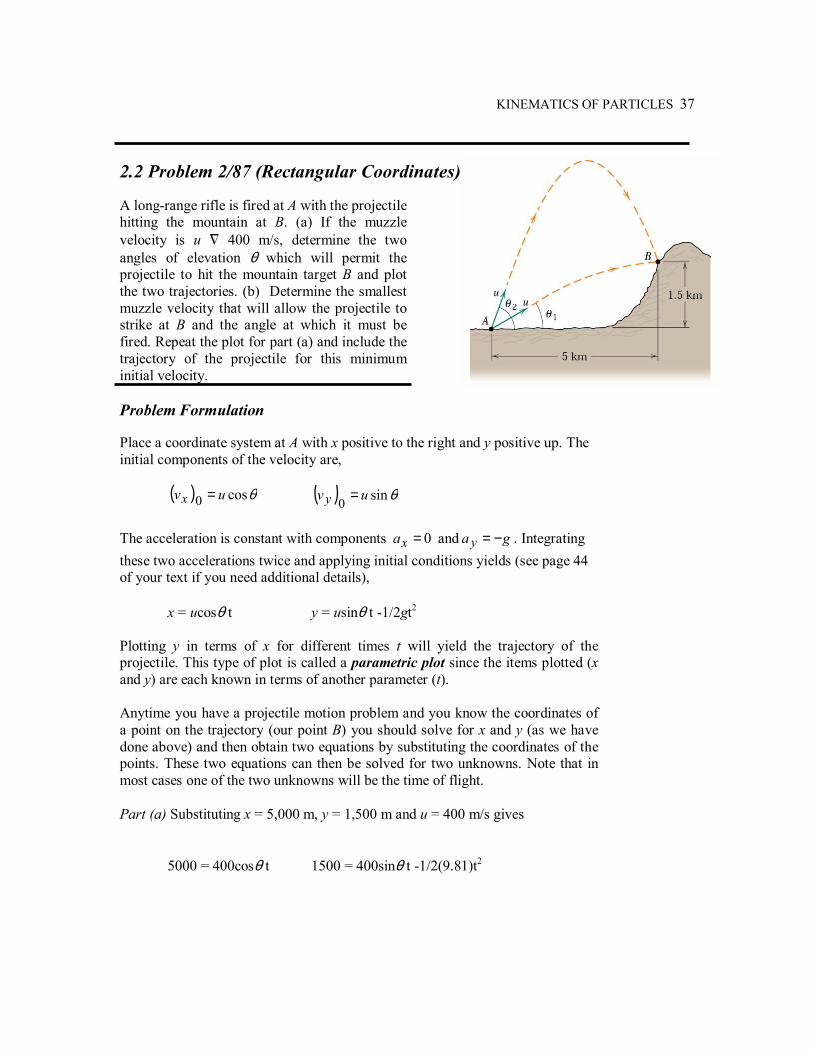
2.2 Problem 2/87 (Rectangular Coordinates) A long-range rifle is fired at A with the projectile hitting the mountain at B. (a) If the muzzle velocity is u 400 m/s, determine the two angles of elevation θ which will permit the projectile to hit the mountain target B and plot the two trajectories. (b) Determine the smallest muzzle velocity that will allow the projectile to strike at B and the angle at which it must be fired. Repeat the plot for part (a) and include the trajectory of the projectile for this minimum initial velocity. Problem Formulation Place a coordinate system at A with x positive to the right and y positive up. The initial components of the velocity are, ( ) θcos0 uvx = ( ) θsin0 uv y =
The acceleration is constant with components 0=xa and ga y −= . Integrating these two accelerations twice and applying initial conditions yields (see page 44 of your text if you need additional details),
x = ucosθ t y = usinθ t -1/2gt2 Plotting y in terms of x for different times t will yield the trajectory of the projectile. This type of plot is called a parametric plot since the items plotted (x and y) are each known in terms of another parameter (t). Anytime you have a projectile motion problem and you know the coordinates of a point on the trajectory (our point B) you should solve for x and y (as we have done above) and then obtain two equations by substituting the coordinates of the points. These two equations can then be solved for two unknowns. Note that in most cases one of the two unknowns will be the time of flight. Part (a) Substituting x = 5,000 m, y = 1,500 m and u = 400 m/s gives
5000 = 400cosθ t 1500 = 400sinθ t -1/2(9.81)t2
38 CH. 2 KINEMATICS OF PARTICLES
We will let MathCad solve these two equations simultaneously. MathCad actually finds four solutions, however two of the four can be discarded since they involve negative times. The other two solutions correspond to the two solutions shown in the illustration accompanying the problem statement. The results are, θ1 = 26.6° and θ2 = 80.6° Part (b) It should be intuitively obvious why there must be a minimum initial velocity below which the projectile cannot reach B. How do we go about finding it? We still have the two equations for the coordinates of point B,
5000 = ucosθ t 1500 = usinθ t -1/2(9.81)t2 however there are now three unknowns (u, θ, t). Suppose for the moment that the launch angle θ were given and we were asked to calculate the required initial speed u so that the projectile strikes B. In this case we would have two equations and two unknowns. From this observation we see that u is a function of θ from which we get our general solution strategy:
(a) Eliminate t from the above two equations and solve for u as a function of θ.
(b) Differentiate this function with respect to θ to find the location of the minimum.
Solving the first equation for u gives
θcos5000
tu =
Substituting into the second yields 221tan50001500 gt−= θ . This equation is
now solved for ( ) gt /1500tan50002 −= θ which can be substituted back into u to give
( ) g
u/1500tan50002cos
5000−
=θθ
We will let MathCad differentiate this equation and solve for the minimum speed and the associated launch angle. The result is umin = 256.8 m/s at θ = 53.3°
KINEMATICS OF PARTICLES 39
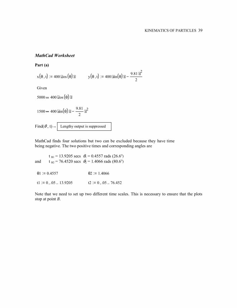
MathCad Worksheet Part (a)
x θ t,( ) 400 cos θ( )⋅ t⋅:= y θ t,( ) 400 sin θ( )⋅ t⋅9.81 t2⋅
2−:=
Given
5000 400 cos θ( )⋅ t⋅
1500 400 sin θ( )⋅ t⋅9.81
2t2⋅−
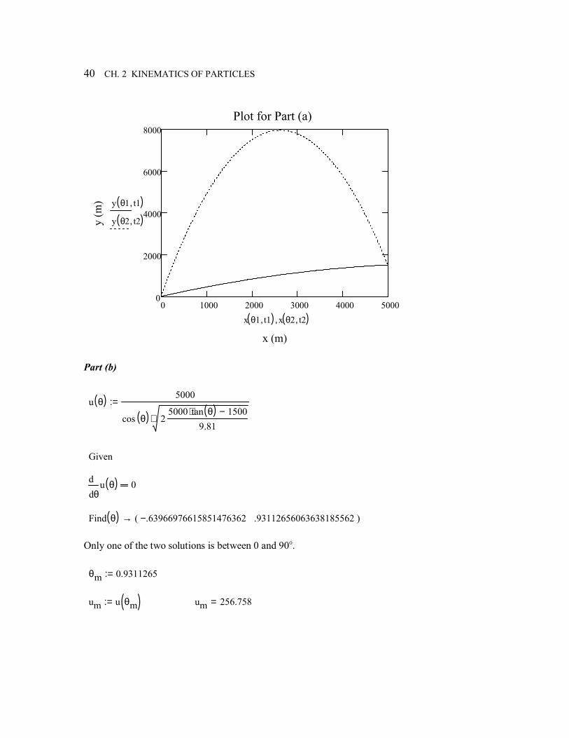
Find(θ , t)→ MathCad finds four solutions but two can be excluded because they have time being negative. The two positive times and corresponding angles are t B1 = 13.9205 secs θ1 = 0.4557 rads (26.6°) and t B2 = 76.4520 secs θ2 = 1.4066 rads (80.6°) θ1 0.4557:= θ2 1.4066:=
t1 0 .05, 13.9205..:= t2 0 .05, 76.452..:= Note that we need to set up two different time scales. This is necessary to ensure that the plots stop at point B.
Lengthy output is suppressed
40 CH. 2 KINEMATICS OF PARTICLES
0 1000 2000 3000 4000 50000
2000
4000
6000
8000Plot for Part (a)
x (m)
y (m
) y θ1 t1,( )y θ2 t2,( )
x θ1 t1,( ) x θ2 t2,( ),
Part (b)
u θ( ) 5000
cos θ( ) 25000 tan θ( )⋅ 1500−
9.81⋅
:=
Given
θu θ( )d
d0
Find θ( ) .63966976615851476362− .93112656063638185562( )→ Only one of the two solutions is between 0 and 90°. θm 0.9311265:=
um u θm( ):= um 256.758=
KINEMATICS OF PARTICLES 41
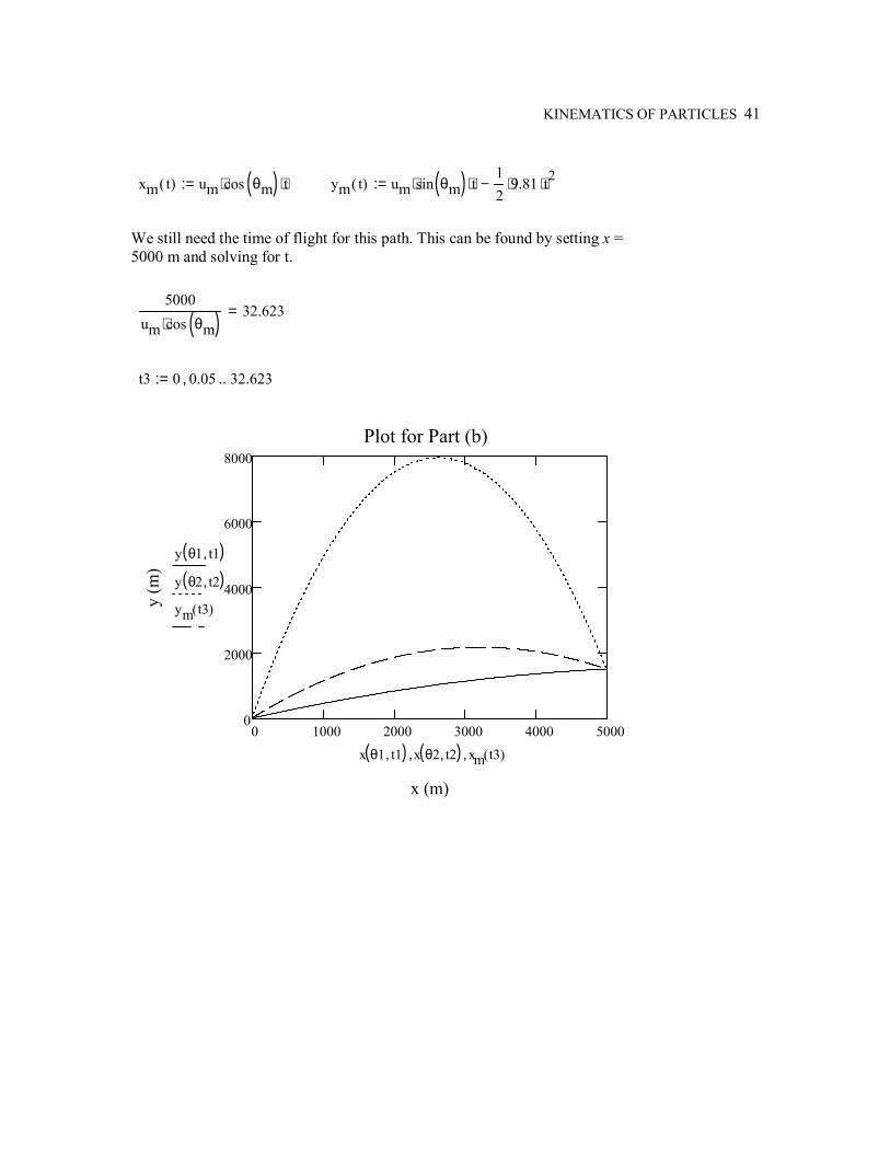
xm t( ) um cos θm( )⋅ t⋅:= ym t( ) um sin θm( )⋅ t⋅12
9.81⋅ t2⋅−:=
We still need the time of flight for this path. This can be found by setting x = 5000 m and solving for t.
5000um cos θm( )⋅
32.623=
t3 0 0.05, 32.623..:=
0 1000 2000 3000 4000 50000
2000
4000
6000
8000Plot for Part (b)
x (m)
y (m
)
y θ1 t1,( )y θ2 t2,( )ym t3( )
x θ1 t1,( ) x θ2 t2,( ), xm t3( ),
42 CH. 2 KINEMATICS OF PARTICLES
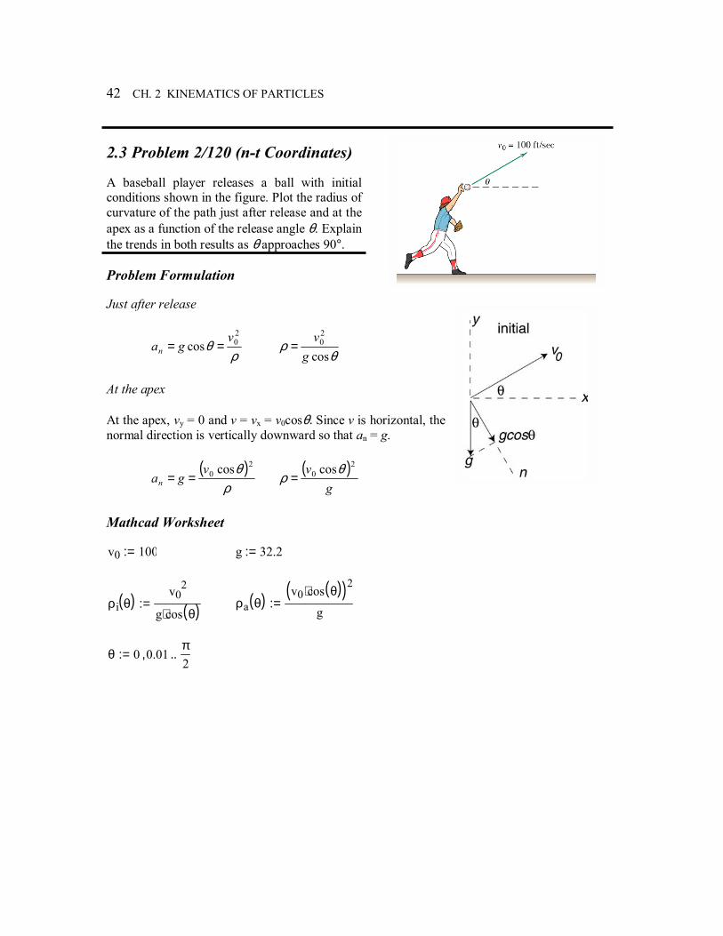
2.3 Problem 2/120 (n-t Coordinates) A baseball player releases a ball with initial conditions shown in the figure. Plot the radius of curvature of the path just after release and at the apex as a function of the release angle θ. Explain the trends in both results as θ approaches 90°. Problem Formulation Just after release
ρθ
20cos
vgan ==
θρ
cos
20
gv
=
At the apex At the apex, vy = 0 and v = vx = v0cosθ. Since v is horizontal, the normal direction is vertically downward so that an = g.
( )
ρθ 2
0 cosvgan ==
( )g
v 20 cosθ
ρ =
Mathcad Worksheet v0 100:= g 32.2:=
ρi θ( ) v02
g cos θ( )⋅:= ρa θ( ) v0 cos θ( )⋅( )2
g:=
θ 0 0.01,π2
..:=
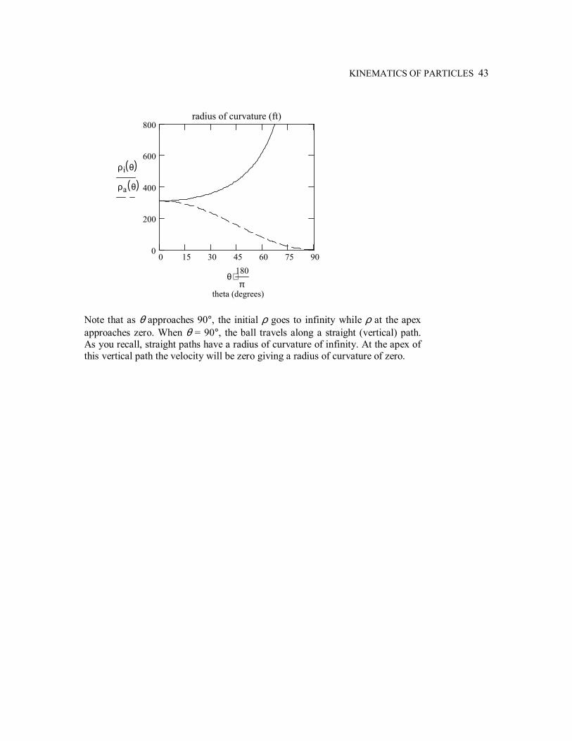
KINEMATICS OF PARTICLES 43
0 15 30 45 60 75 900
200
400
600
800radius of curvature (ft)
theta (degrees)
ρi θ( )
ρa θ( )
θ180π
⋅
Note that as θ approaches 90°, the initial ρ goes to infinity while ρ at the apex approaches zero. When θ = 90°, the ball travels along a straight (vertical) path. As you recall, straight paths have a radius of curvature of infinity. At the apex of this vertical path the velocity will be zero giving a radius of curvature of zero.
44 CH. 2 KINEMATICS OF PARTICLES
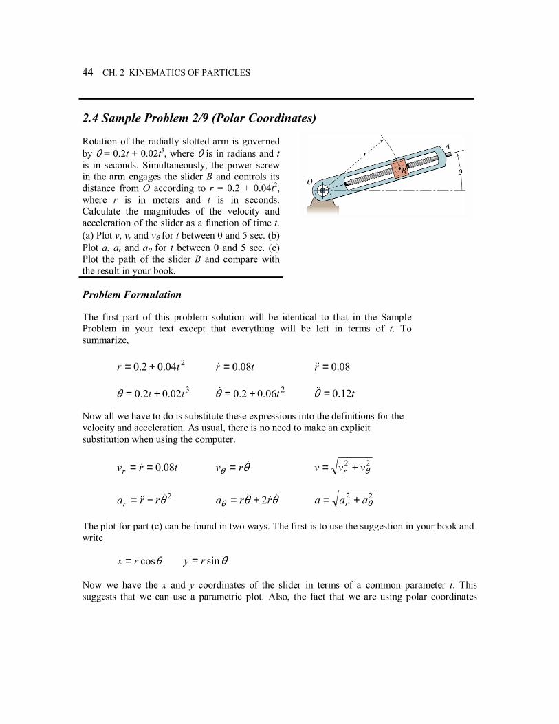
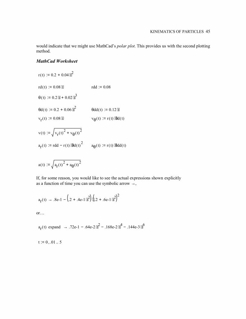
2.4 Sample Problem 2/9 (Polar Coordinates) Rotation of the radially slotted arm is governed by θ = 0.2t + 0.02t3, where θ is in radians and t is in seconds. Simultaneously, the power screw in the arm engages the slider B and controls its distance from O according to r = 0.2 + 0.04t2, where r is in meters and t is in seconds. Calculate the magnitudes of the velocity and acceleration of the slider as a function of time t. (a) Plot v, vr and vθ for t between 0 and 5 sec. (b) Plot a, ar and aθ for t between 0 and 5 sec. (c) Plot the path of the slider B and compare with the result in your book. Problem Formulation The first part of this problem solution will be identical to that in the Sample Problem in your text except that everything will be left in terms of t. To summarize,
204.02.0 tr += tr 08.0=& 08.0=r&&
302.02.0 tt +=θ 206.02.0 t+=θ& t12.0=θ&& Now all we have to do is substitute these expressions into the definitions for the velocity and acceleration. As usual, there is no need to make an explicit substitution when using the computer.
trvr 08.0== & θθ&rv = 22
θvvv r +=
2θ&&& rrar −= θθθ&&&& rra 2+= 22
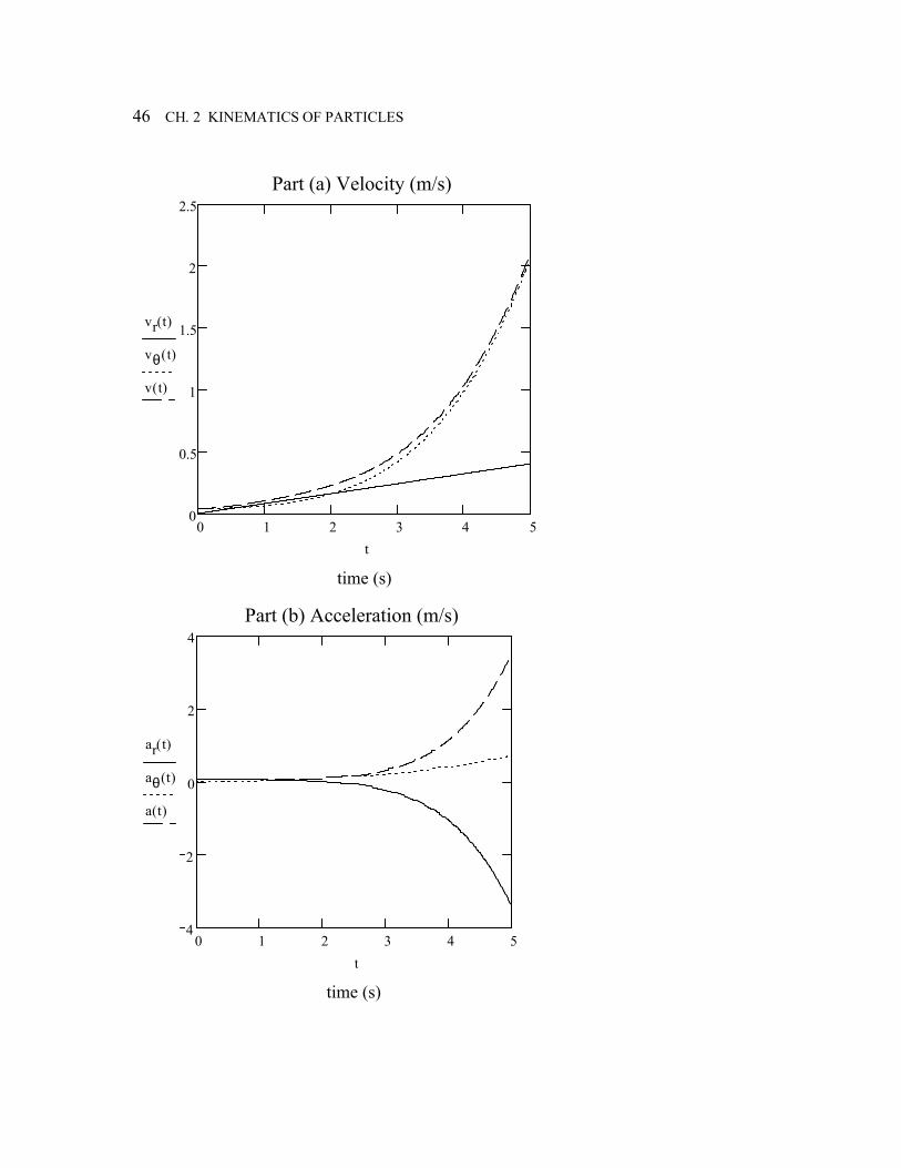
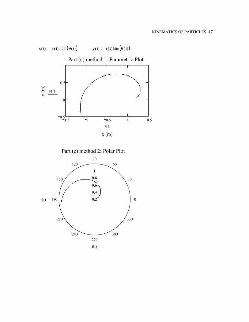
θaaa r += The plot for part (c) can be found in two ways. The first is to use the suggestion in your book and write θcosrx = θsinry = Now we have the x and y coordinates of the slider in terms of a common parameter t. This suggests that we can use a parametric plot. Also, the fact that we are using polar coordinates
KINEMATICS OF PARTICLES 45
would indicate that we might use MathCads polar plot. This provides us with the second plotting method. MathCad Worksheet
r t( ) 0.2 0.04 t2⋅+:=
rd t( ) 0.08 t⋅:= rdd 0.08:=
θ t( ) 0.2 t⋅ 0.02 t3⋅+:=
θd t( ) 0.2 0.06 t2⋅+:= θdd t( ) 0.12 t⋅:= vr t( ) 0.08 t⋅:= vθ t( ) r t( ) θd t( )⋅:=
v t( ) vr t( )2 vθ t( )2+:=
ar t( ) rdd r t( ) θd t( )2⋅−:= aθ t( ) r t( ) θdd t( )⋅:=
a t( ) ar t( )2 aθ t( )2+:=
If, for some reason, you would like to see the actual expressions shown explicitly as a function of time you can use the symbolic arrow →,
ar t( ) .8e-1 .2 .4e-1 t2⋅+( ) .2 .6e-1 t2⋅+( )2⋅−→
or
ar t( ) expand .72e-1 .64e-2 t2⋅− .168e-2 t4⋅− .144e-3 t6⋅−→
t 0 .01, 5..:=
46 CH. 2 KINEMATICS OF PARTICLES
0 1 2 3 4 50
0.5
1
1.5
2
2.5Part (a) Velocity (m/s)
time (s)
vr t( )
vθ t( )
v t( )
t
0 1 2 3 4 54
2
0
2
4Part (b) Acceleration (m/s)
time (s)
ar t( )
aθ t( )
a t( )
t
KINEMATICS OF PARTICLES 47
x t( ) r t( ) cos θ t( )( )⋅:= y t( ) r t( ) sin θ t( )( )⋅:=
1.5 1 0.5 0 0.50.5
0
0.5
1Part (c) method 1: Parametric Plot
x (m)
y (m
)
y t( )
x t( )
0
30
6090
120
150
180
210
240270
300
330
1
0.8
0.6
0.4
0.2
Part (c) method 2: Polar Plot
r t( )
θ t( )
48 CH. 2 KINEMATICS OF PARTICLES
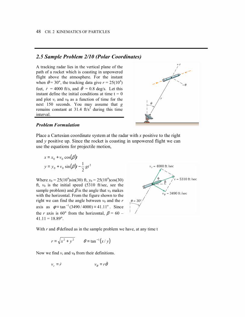
2.5 Sample Problem 2/10 (Polar Coordinates) A tracking radar lies in the vertical plane of the path of a rocket which is coasting in unpowered flight above the atmosphere. For the instant when θ = 30°, the tracking data give r = 25(104) feet, r& = 4000 ft/s, and θ& = 0.8 deg/s. Let this instant define the initial conditions at time t = 0 and plot vr and vθ as a function of time for the next 150 seconds. You may assume that g remains constant at 31.4 ft/s2 during this time interval. Problem Formulation Place a Cartesian coordinate system at the radar with x positive to the right and y positive up. Since the rocket is coasting in unpowered flight we can use the equations for projectile motion, ( )tvxx βcos00 +=
( ) 200 2
1sin gttvyy −+= β
Where x0 = 25(104)sin(30) ft, y0 = 25(104)cos(30) ft, v0 is the initial speed (5310 ft/sec, see the sample problem) and β is the angle that v0 makes with the horizontal. From the figure shown to the right we can find the angle between v0 and the r axis as o1 11.41)4000/3490(tan == −φ . Since the r axis is 60° from the horizontal, β = 60 41.11 = 18.89°. With r and θ defined as in the sample problem we have, at any time t 22 yxr += ( )yx /tan 1−=θ Now we find vr and vθ from their definitions. rvr &= θθ
&rv =
KINEMATICS OF PARTICLES 49
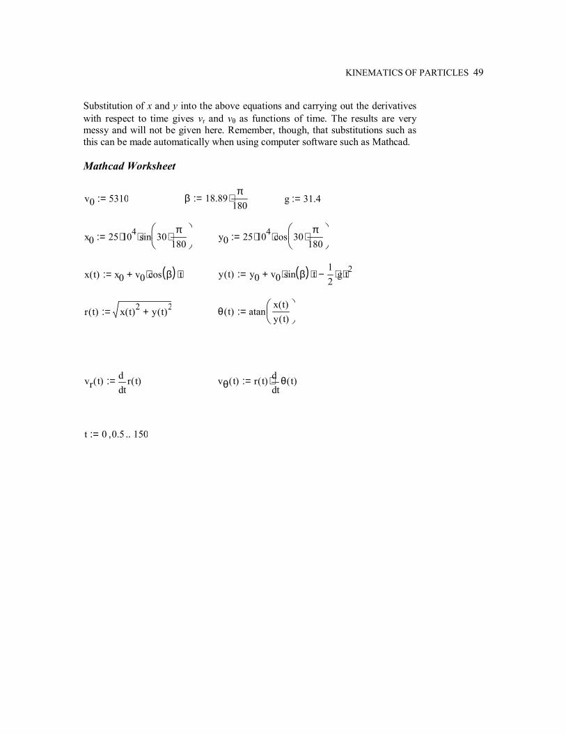
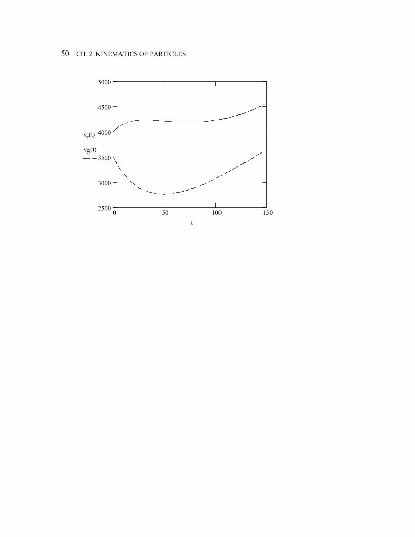
Substitution of x and y into the above equations and carrying out the derivatives with respect to time gives vr and vθ as functions of time. The results are very messy and will not be given here. Remember, though, that substitutions such as this can be made automatically when using computer software such as Mathcad. Mathcad Worksheet
v0 5310:= β 18.89π
180⋅:= g 31.4:=
x0 25 104⋅ sin 30π
180⋅
⋅:= y0 25 104⋅ cos 30π
180⋅
⋅:=
x t( ) x0 v0 cos β( )⋅ t⋅+:= y t( ) y0 v0 sin β( )⋅ t⋅+12
g⋅ t2⋅−:=
r t( ) x t( )2 y t( )2+:= θ t( ) atanx t( )y t( )
:=
vr t( )tr t( )d
d:= vθ t( ) r t( )
tθ t( )d
d⋅:=
t 0 0.5, 150..:=
50 CH. 2 KINEMATICS OF PARTICLES
0 50 100 1502500
3000
3500
4000
4500
5000
vr t( )
vθ t( )
t
KINEMATICS OF PARTICLES 51
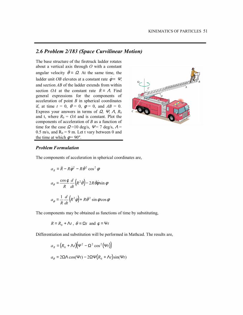
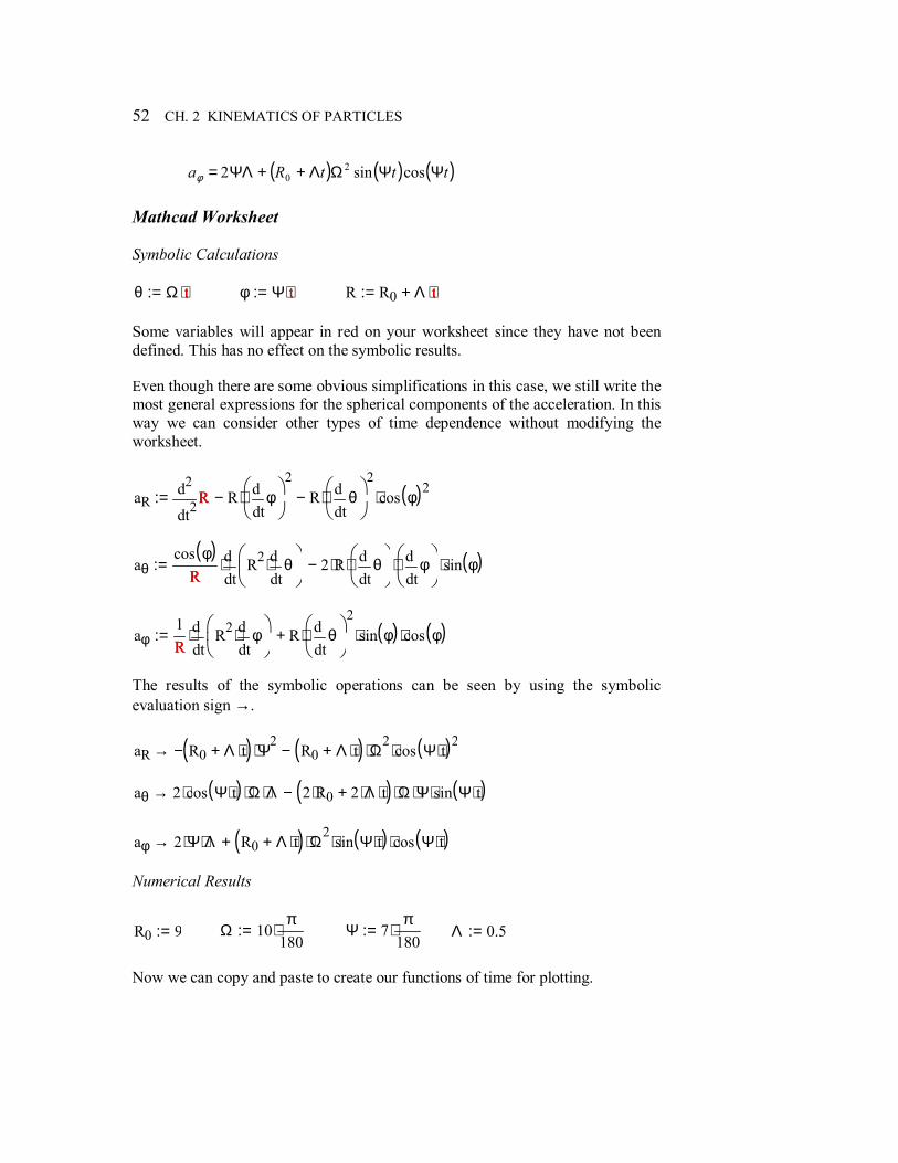
2.6 Problem 2/183 (Space Curvilinear Motion) The base structure of the firetruck ladder rotates about a vertical axis through O with a constant angular velocity =θ& Ω. At the same time, the ladder unit OB elevates at a constant rate =φ& Ψ, and section AB of the ladder extends from within section OA at the constant rate =R& Λ. Find general expressions for the components of acceleration of point B in spherical coordinates if, at time t = 0, θ = 0, φ = 0, and AB = 0. Express your answers in terms of Ω, Ψ, Λ, R0 and t, where R0 = OA and is constant. Plot the components of acceleration of B as a function of time for the case Ω =10 deg/s, Ψ = 7 deg/s, Λ = 0.5 m/s, and R0 = 9 m. Let t vary between 0 and the time at which φ = 90°. Problem Formulation The components of acceleration in spherical coordinates are, φθφ 222 cos&&&& RRRaR −−=
( ) φφθθφθ sin2cos 2 &&& RR
dtd
Ra −=
( ) φφθφφ cossin1 22 && RRdtd
Ra +=
The components may be obtained as functions of time by substituting,
tRR Λ+= 0 , tΩ=θ and tΨ=φ
Differentiation and substitution will be performed in Mathcad. The results are, ( ) ( )( )ttRaR ΨΩ−ΨΛ+= 222
0 cos ( ) )sin(2)cos(2 0 ttRta ΨΛ+ΩΨ−ΨΩΛ=θ
52 CH. 2 KINEMATICS OF PARTICLES
( ) ( ) ( )tttRa ΨΨΩΛ++ΨΛ= cossin2 20φ
Mathcad Worksheet Symbolic Calculations θ Ω t⋅:= t φ Ψ t⋅:= t R R0 Λ t⋅+:= t Some variables will appear in red on your worksheet since they have not been defined. This has no effect on the symbolic results. Even though there are some obvious simplifications in this case, we still write the most general expressions for the spherical components of the acceleration. In this way we can consider other types of time dependence without modifying the worksheet.
aR 2tRd
d
2R
tφd
d
2⋅− R
tθd
d
2⋅ cos φ( )2
⋅−:= R
aθcos φ( )
R tR2
tθd
d⋅
dd
⋅ 2 R⋅tθd
d
⋅tφd
d
⋅ sin φ( )⋅−:=R
aφ1R t
R2tφd
d⋅
dd
⋅ Rtθd
d
2⋅ sin φ( )⋅ cos φ( )⋅+:=
R The results of the symbolic operations can be seen by using the symbolic evaluation sign →.
aR R0 Λ t⋅+( )− Ψ2
⋅ R0 Λ t⋅+( ) Ω2
⋅ cos Ψ t⋅( )2⋅−→
aθ 2 cos Ψ t⋅( )⋅ Ω⋅ Λ⋅ 2 R0⋅ 2 Λ⋅ t⋅+( ) Ω⋅ Ψ⋅ sin Ψ t⋅( )⋅−→
aφ 2 Ψ⋅ Λ⋅ R0 Λ t⋅+( ) Ω2
⋅ sin Ψ t⋅( )⋅ cos Ψ t⋅( )⋅+→ Numerical Results
R0 9:= Ω 10π
180⋅:= Ψ 7
π180
⋅:= Λ 0.5:=
Now we can copy and paste to create our functions of time for plotting.
KINEMATICS OF PARTICLES 53
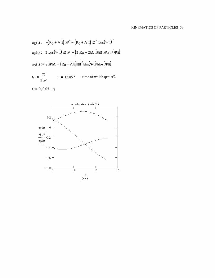
aR t( ) R0 Λ t⋅+( )− Ψ2
⋅ R0 Λ t⋅+( ) Ω2
⋅ cos Ψ t⋅( )2⋅−:=
aθ t( ) 2 cos Ψ t⋅( )⋅ Ω⋅ Λ⋅ 2 R0⋅ 2 Λ⋅ t⋅+( ) Ω⋅ Ψ⋅ sin Ψ t⋅( )⋅−:=
aφ t( ) 2 Ψ⋅ Λ⋅ R0 Λ t⋅+( ) Ω2
⋅ sin Ψ t⋅( )⋅ cos Ψ t⋅( )⋅+:=
tfπ
2 Ψ⋅:= tf 12.857= time at which φ = π/2.
t 0 0.05, tf..:=
0 5 10 150.8
0.6
0.4
0.2
0
0.2
acceleration (m/s^2)
(sec)
aR t( )
aθ t( )
aφ t( )
t
54 CH. 2 KINEMATICS OF PARTICLES
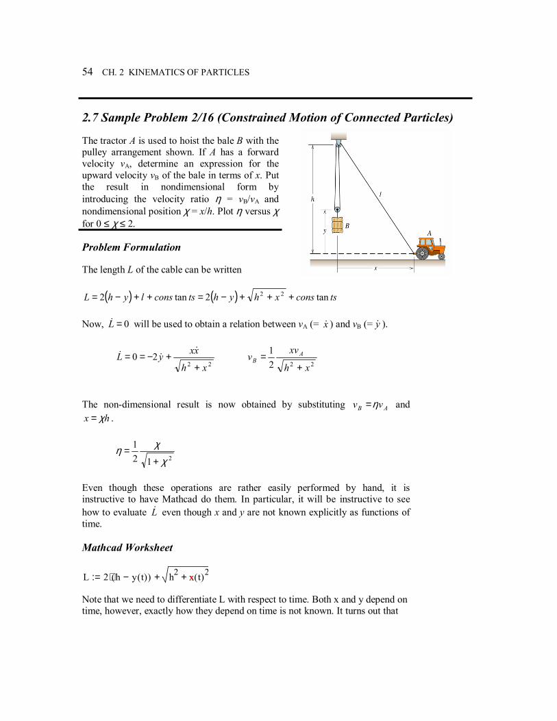
2.7 Sample Problem 2/16 (Constrained Motion of Connected Particles) The tractor A is used to hoist the bale B with the pulley arrangement shown. If A has a forward velocity vA, determine an expression for the upward velocity vB of the bale in terms of x. Put the result in nondimensional form by introducing the velocity ratio η = vB/vA and nondimensional position χ = x/h. Plot η versus χ for 0 ≤ χ ≤ 2. Problem Formulation The length L of the cable can be written
( ) ( ) tsconsxhyhtsconslyhL tan2tan2 22 +++−=++−= Now, 0=L& will be used to obtain a relation between vA (= x& ) and vB (= y& ).
2220
xh
xxyL+
+−==&
&& 222
1
xh
xvv A
B+
=
The non-dimensional result is now obtained by substituting AB vv η= and
hx χ= .
212
1
χ
χη+
=
Even though these operations are rather easily performed by hand, it is instructive to have Mathcad do them. In particular, it will be instructive to see how to evaluate L& even though x and y are not known explicitly as functions of time. Mathcad Worksheet
L 2 h y t( )−( )⋅ h2 x t( )2++:= x Note that we need to differentiate L with respect to time. Both x and y depend on time, however, exactly how they depend on time is not known. It turns out that
KINEMATICS OF PARTICLES 55
this is not a problem. All we need to do is let Mathcad know x and y depend on time by writing x(t) and y(t).
LdottLd
d:= L
Ldot 2−ty t( )d
d⋅
1
h2 x t( )2+( )12
x t( )⋅tx t( )d
d⋅+→
Now we make our substitutions. The first substitutes vB = ηvA for y& (= )(tydtd ).
Ldot
substitutety t( )d
dη vA⋅,
substitutetx t( )d
dvA,
substitute x t( ) χ h⋅,
2− η⋅ vA⋅1
h2 χ2
h2⋅+( )12
χ⋅ h⋅ vA⋅+→
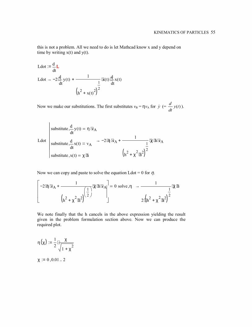
Now we can copy and paste to solve the equation Ldot = 0 for η.
2− η⋅ vA⋅1
h2 χ2
h2⋅+( )12
χ⋅ h⋅ vA⋅+
0 solve η,1
2 h2 χ2
h2⋅+( )12
⋅
χ⋅ h⋅→
We note finally that the h cancels in the above expression yielding the result given in the problem formulation section above. Now we can produce the required plot.
η χ( ) 12
χ
1 χ2
+⋅:=
χ 0 0.01, 2..:=
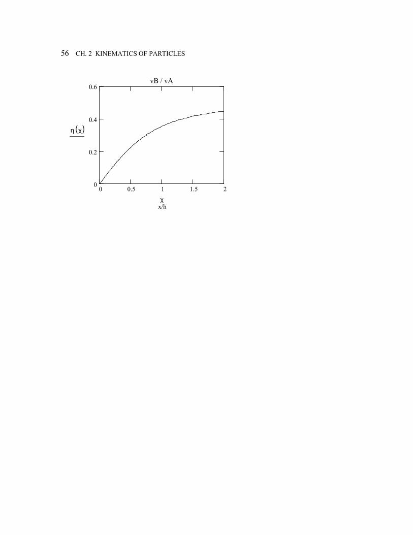
56 CH. 2 KINEMATICS OF PARTICLES
0 0.5 1 1.5 20
0.2
0.4
0.6vB / vA
x/h
η χ( )
χ
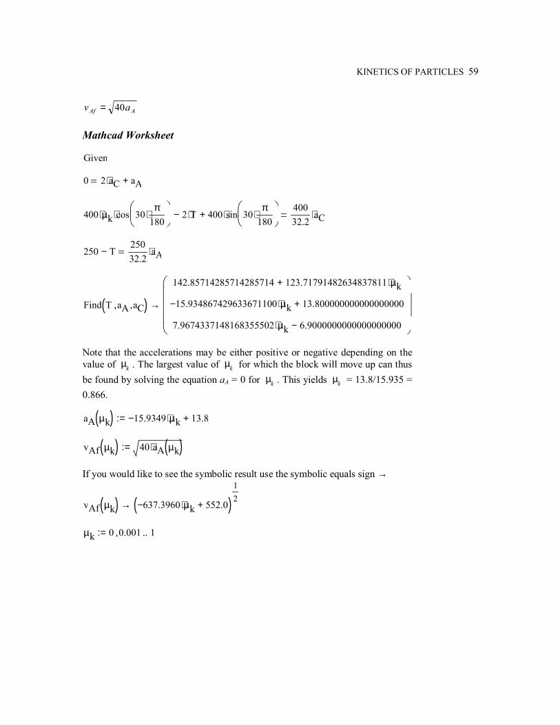
KINETICS OF PARTICLES The kinetics of particles is concerned with the motion produced by unbalanced forces acting on a particle. This chapter considers three approaches to the solution of particle kinetics problems: (1) direct application of Newtons second law, (2) work and energy, and (3) impulse and momentum. Problem 3.1 is a rectilinear motion problem where three equations are solved symbolically for three unknowns. In problem 3.2, polar plotting is used to plot the absolute path of a particle. This problem also illustrates how Mathcad can be used to solve a second order differential equation with initial conditions numerically. Problem 3.3 uses Mathcad to study the effect of initial spring stretch upon the velocity of a slider. A physical interpretation of the results is also required. Problem 3.4 is a typical ballistic pendulum problem requiring both work/energy and conservation of momentum to relate the velocity of a projectile to the maximum swing angle of a pendulum. Problem 3.5 is a relatively straightforward conservation of angular momentum problem where Mathcad is used to generate a plot that might be useful in a parametric study. In problem 3.6, two equations are solved symbolically for two unknowns using GivenFind. The maximum value of a function is then determined.
3
58 CH. 3 KINETICS OF PARTICLES
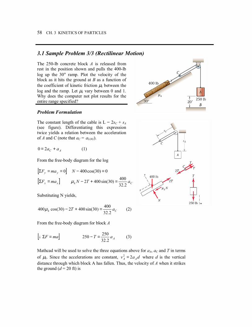
3.1 Sample Problem 3/3 (Rectilinear Motion) The 250-lb concrete block A is released from rest in the position shown and pulls the 400-lb log up the 30° ramp. Plot the velocity of the block as it hits the ground at B as a function of the coefficient of kinetic friction µk between the log and the ramp. Let µk vary between 0 and 1. Why does the computer not plot results for the entire range specified? Problem Formulation The constant length of the cable is L = 2sC + sA (see figure). Differentiating this expression twice yields a relation between the acceleration of A and C (note that aC = aLOG).
AC aa += 20 (1) From the free-body diagram for the log [ ]0==Σ yy maF 0)30cos(400 =−N
[ ]xx maF =Σ Ck aTN2.32
400)30sin(4002 =+−µ
Substituting N yields,
Ck aT2.32
400)30sin(4002)30cos(400 =+−µ (2)
From the free-body diagram for block A
[ ]maF =Σ↓ AaT2.32
250250 =− (3)
Mathcad will be used to solve the three equations above for aA, aC and T in terms of µk. Since the accelerations are constant, dav AA 22 = where d is the vertical distance through which block A has fallen. Thus, the velocity of A when it strikes the ground (d = 20 ft) is
KINETICS OF PARTICLES 59
AAf av 40= Mathcad Worksheet Given 0 2 aC⋅ aA+
400 µk⋅ cos 30π
180⋅
⋅ 2 T⋅− 400 sin 30π
180⋅
⋅+40032.2
aC⋅
250 T−25032.2
aA⋅
Find T aA, aC,( )142.85714285714285714 123.71791482634837811 µk⋅+
15.934867429633671100− µk⋅ 13.800000000000000000+
7.9674337148168355502 µk⋅ 6.9000000000000000000−
→
Note that the accelerations may be either positive or negative depending on the value of µk . The largest value of µk for which the block will move up can thus be found by solving the equation aA = 0 for µk . This yields µk = 13.8/15.935 = 0.866. aA µk( ) 15.9349− µk⋅ 13.8+:=
vAf µk( ) 40 aA µk( )⋅:=
If you would like to see the symbolic result use the symbolic equals sign →
vAf µk( ) 637.3960− µk⋅ 552.0+( )12
→ µk 0 0.001, 1..:=
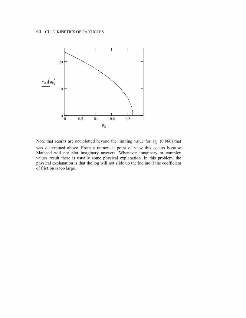
60 CH. 3 KINETICS OF PARTICLES
0 0.2 0.4 0.6 0.8 10
10
20
vAf µk( )
µk
Note that results are not plotted beyond the limiting value for µk (0.866) that was determined above. From a numerical point of view this occurs because Mathcad will not plot imaginary answers. Whenever imaginary or complex values result there is usually some physical explanation. In this problem, the physical explanation is that the log will not slide up the incline if the coefficient of friction is too large.
KINETICS OF PARTICLES 61
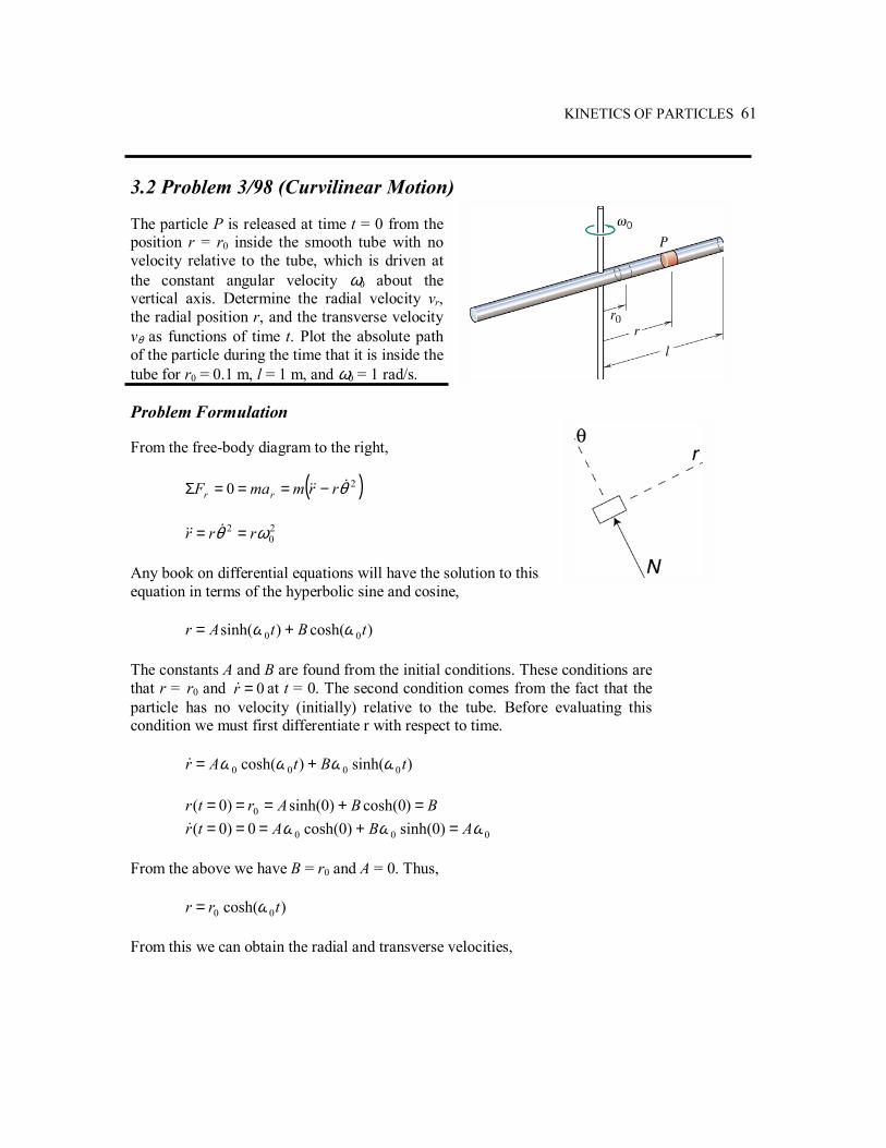
3.2 Problem 3/98 (Curvilinear Motion) The particle P is released at time t = 0 from the position r = r0 inside the smooth tube with no velocity relative to the tube, which is driven at the constant angular velocity ω0 about the vertical axis. Determine the radial velocity vr, the radial position r, and the transverse velocity vθ as functions of time t. Plot the absolute path of the particle during the time that it is inside the tube for r0 = 0.1 m, l = 1 m, and ω0 = 1 rad/s. Problem Formulation From the free-body diagram to the right, ( )20 θ&&& rrmmaF rr −===Σ 2
02 ωθ rrr == &&&
Any book on differential equations will have the solution to this equation in terms of the hyperbolic sine and cosine, )cosh()sinh( 00 tBtAr ωω += The constants A and B are found from the initial conditions. These conditions are that r = r0 and 0=r& at t = 0. The second condition comes from the fact that the particle has no velocity (initially) relative to the tube. Before evaluating this condition we must first differentiate r with respect to time. )sinh()cosh( 0000 tBtAr ωωωω +=& BBArtr =+=== )0cosh()0sinh()0( 0 000 )0sinh()0cosh(0)0( ωωω ABAtr =+===& From the above we have B = r0 and A = 0. Thus, )cosh( 00 trr ω= From this we can obtain the radial and transverse velocities,
62 CH. 3 KINETICS OF PARTICLES
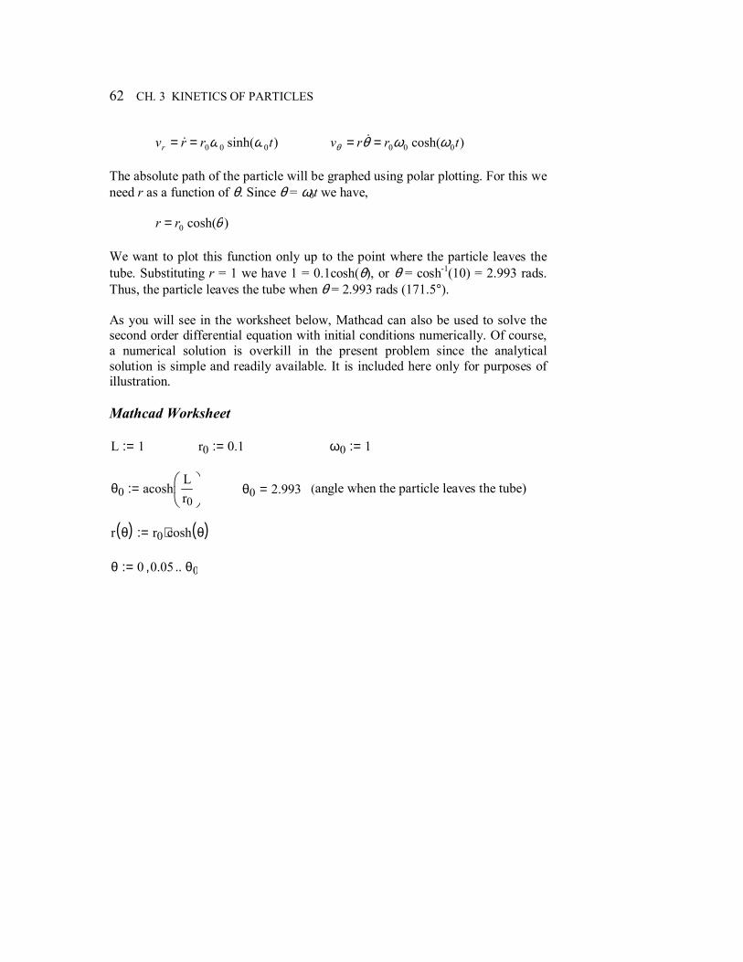
)sinh( 000 trrvr ωω== & )cosh( 000 trrv ωωθθ == & The absolute path of the particle will be graphed using polar plotting. For this we need r as a function of θ. Since θ = ω0t we have, )cosh(0 θrr = We want to plot this function only up to the point where the particle leaves the tube. Substituting r = 1 we have 1 = 0.1cosh(θ), or θ = cosh-1(10) = 2.993 rads. Thus, the particle leaves the tube when θ = 2.993 rads (171.5°). As you will see in the worksheet below, Mathcad can also be used to solve the second order differential equation with initial conditions numerically. Of course, a numerical solution is overkill in the present problem since the analytical solution is simple and readily available. It is included here only for purposes of illustration. Mathcad Worksheet L 1:= r0 0.1:= ω0 1:=
θ0 acoshLr0
:= θ0 2.993= (angle when the particle leaves the tube)
r θ( ) r0 cosh θ( )⋅:= θ 0 0.05, θ0..:=
KINETICS OF PARTICLES 63
0
30
6090
120
150
180
210
240270
300
330
0.80.60.40.20
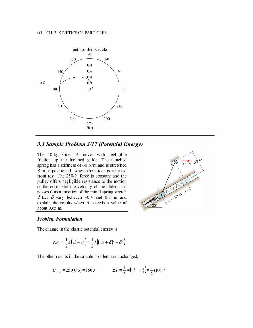
path of the particle
r θ( )
θ
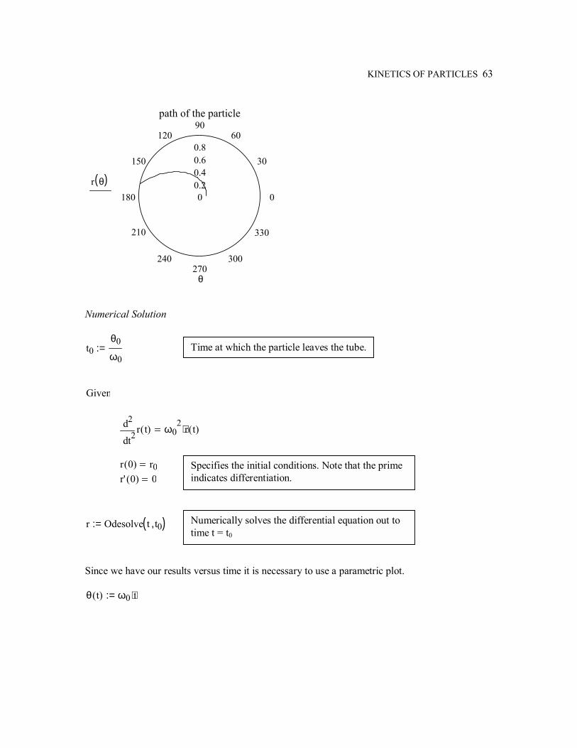
Numerical Solution
t0θ0
ω0:=
Given
2tr t( )d
d
2ω0
2r t( )⋅
r 0( ) r0 r' 0( ) 0
r Odesolve t t0,( ):= Since we have our results versus time it is necessary to use a parametric plot. θ t( ) ω0 t⋅:=
Specifies the initial conditions. Note that the prime indicates differentiation.
Numerically solves the differential equation out to time t = t0
Time at which the particle leaves the tube.
64 CH. 3 KINETICS OF PARTICLES
0
30
6090
120
150
180
210
240270
300
330
0.80.60.40.20
path of the particle
r t( )
θ t( )
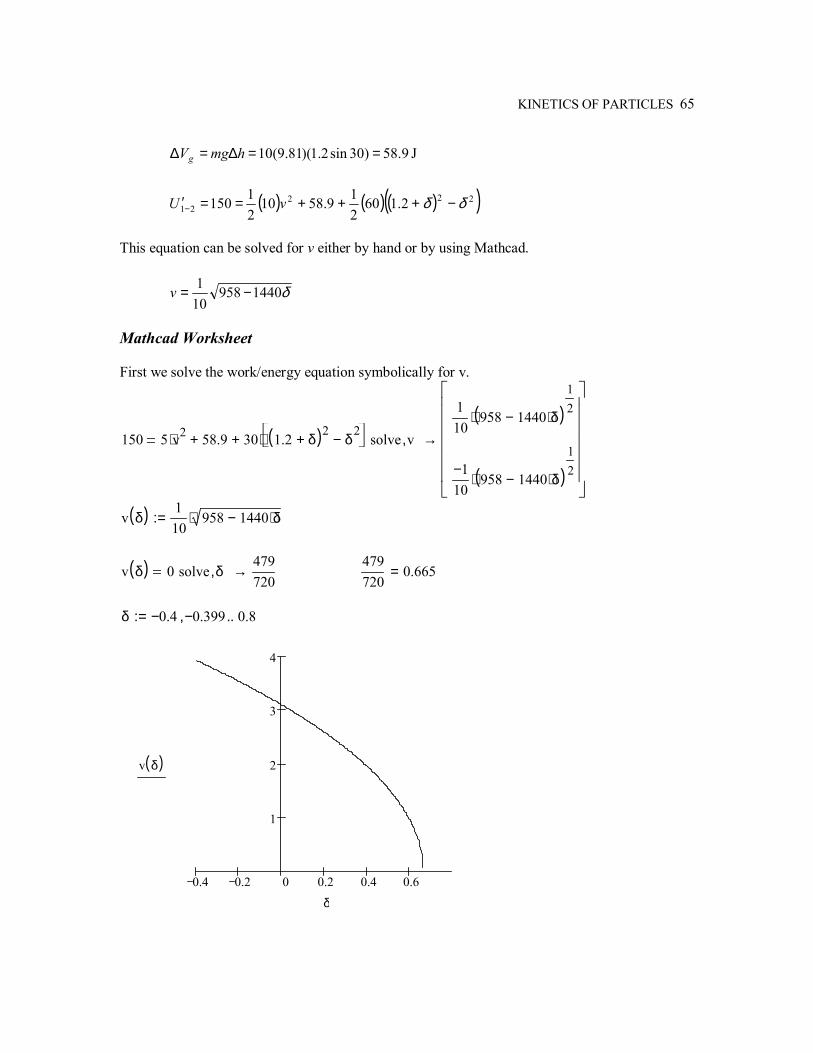
3.3 Sample Problem 3/17 (Potential Energy) The 10-kg slider A moves with negligible friction up the inclined guide. The attached spring has a stiffness of 60 N/m and is stretched δ m at position A, where the slider is released from rest. The 250-N force is constant and the pulley offers negligible resistance to the motion of the cord. Plot the velocity of the slider as it passes C as a function of the initial spring stretch δ. Let δ vary between 0.4 and 0.8 m and explain the results when δ exceeds a value of about 0.65 m. Problem Formulation The change in the elastic potential energy is
( ) ( )( )2221
22 2.1
21
21 δδ −+=−=∆ kxxkVe
The other results in the sample problem are unchanged,
150)6.0(25021 ==′−U J ( ) 220
2 )10(21
21 vvvmT =−=∆
KINETICS OF PARTICLES 65
9.58)30sin2.1)(81.9(10 ==∆=∆ hmgVg J
( ) ( ) ( )( )22221 2.160
219.5810
21150 δδ −+++==′− vU
This equation can be solved for v either by hand or by using Mathcad.
δ1440958101 −=v
Mathcad Worksheet First we solve the work/energy equation symbolically for v.
150 5 v2⋅ 58.9+ 30 1.2 δ+( )2δ
2− ⋅+ solve v,
110
958 1440 δ⋅−( )12
⋅
1−10
958 1440 δ⋅−( )12
⋅
→
v δ( ) 110
958 1440 δ⋅−⋅:=
v δ( ) 0 solve δ,479720
→ 479720
0.665=
δ 0.4− 0.399−, 0.8..:=
0.4 0.2 0 0.2 0.4 0.6
1
2
3
4
v δ( )
δ
66 CH. 3 KINETICS OF PARTICLES
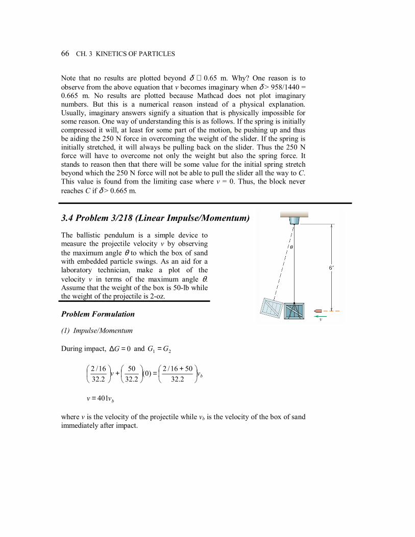
Note that no results are plotted beyond δ ≅ 0.65 m. Why? One reason is to observe from the above equation that v becomes imaginary when δ > 958/1440 = 0.665 m. No results are plotted because Mathcad does not plot imaginary numbers. But this is a numerical reason instead of a physical explanation. Usually, imaginary answers signify a situation that is physically impossible for some reason. One way of understanding this is as follows. If the spring is initially compressed it will, at least for some part of the motion, be pushing up and thus be aiding the 250 N force in overcoming the weight of the slider. If the spring is initially stretched, it will always be pulling back on the slider. Thus the 250 N force will have to overcome not only the weight but also the spring force. It stands to reason then that there will be some value for the initial spring stretch beyond which the 250 N force will not be able to pull the slider all the way to C. This value is found from the limiting case where v = 0. Thus, the block never reaches C if δ > 0.665 m. 3.4 Problem 3/218 (Linear Impulse/Momentum) The ballistic pendulum is a simple device to measure the projectile velocity v by observing the maximum angle θ to which the box of sand with embedded particle swings. As an aid for a laboratory technician, make a plot of the velocity v in terms of the maximum angle θ. Assume that the weight of the box is 50-lb while the weight of the projectile is 2-oz. Problem Formulation (1) Impulse/Momentum During impact, 0=∆G and 21 GG =
bvv
+=
+
2.325016/2)0(
2.3250
2.3216/2
bvv 401= where v is the velocity of the projectile while vb is the velocity of the box of sand immediately after impact.
KINETICS OF PARTICLES 67
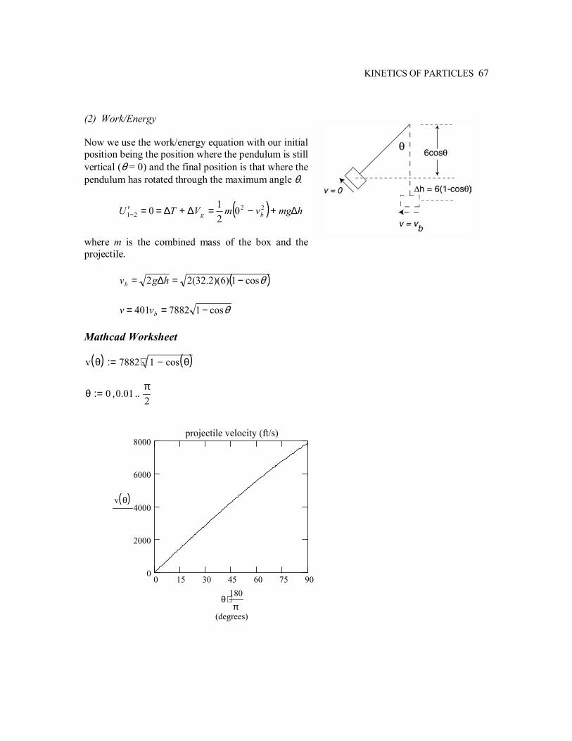
(2) Work/Energy Now we use the work/energy equation with our initial position being the position where the pendulum is still vertical (θ = 0) and the final position is that where the pendulum has rotated through the maximum angle θ.
( ) hmgvmVTU bg ∆+−=∆+∆==′−22
21 0210
where m is the combined mass of the box and the projectile. ( )θcos1)6)(2.32(22 −=∆= hgvb θcos17882401 −== bvv Mathcad Worksheet v θ( ) 7882 1 cos θ( )−⋅:=
θ 0 0.01,π2
..:=
0 15 30 45 60 75 900
2000
4000
6000
8000projectile velocity (ft/s)
(degrees)
v θ( )
θ180π
⋅
68 CH. 3 KINETICS OF PARTICLES
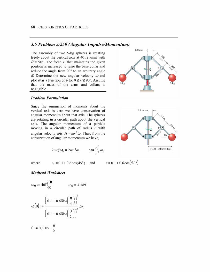
3.5 Problem 3/250 (Angular Impulse/Momentum) The assembly of two 5-kg spheres is rotating freely about the vertical axis at 40 rev/min with θ = 90°. The force F that maintains the given position is increased to raise the base collar and reduce the angle from 90° to an arbitrary angle θ. Determine the new angular velocity ω and plot ω as a function of θ for 0 ≤ θ ≤ 90°. Assume that the mass of the arms and collars is negligible. Problem Formulation Since the summation of moments about the vertical axis is zero we have conservation of angular momentum about that axis. The spheres are rotating in a circular path about the vertical axis. The angular momentum of a particle moving in a circular path of radius r with angular velocity ω is ω2mrH = . Thus, from the conservation of angular momentum we have,
ωω 20
20 22 mrmr = 02
20 ωω
rr
=
where )45cos(6.01.0 0
0 +=r and ( )2/cos6.01.0 θ+=r Mathcad Worksheet
ω0 402 π⋅60
⋅:= ω0 4.189=
ω θ( )0.1 0.6 cos
π4
⋅+
2
0.1 0.6 cosθ2
⋅+
2ω0⋅:=
θ 0 0.05,π2
..:=
KINETICS OF PARTICLES 69
0 15 30 45 60 75 902
2.5
3
3.5
4
4.5angular velocity (rad/s)
(degrees)
ω θ( )
θ180π
⋅
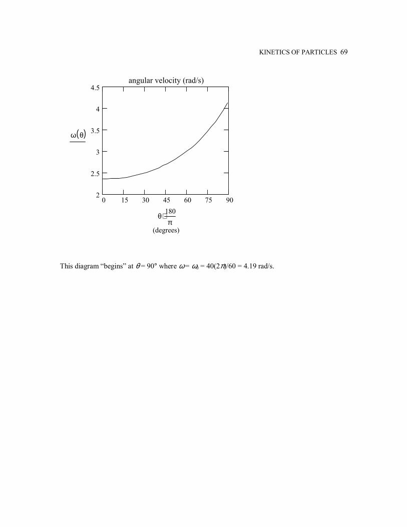
This diagram begins at θ = 90° where ω = ω0 = 40(2π)/60 = 4.19 rad/s.
70 CH. 3 KINETICS OF PARTICLES
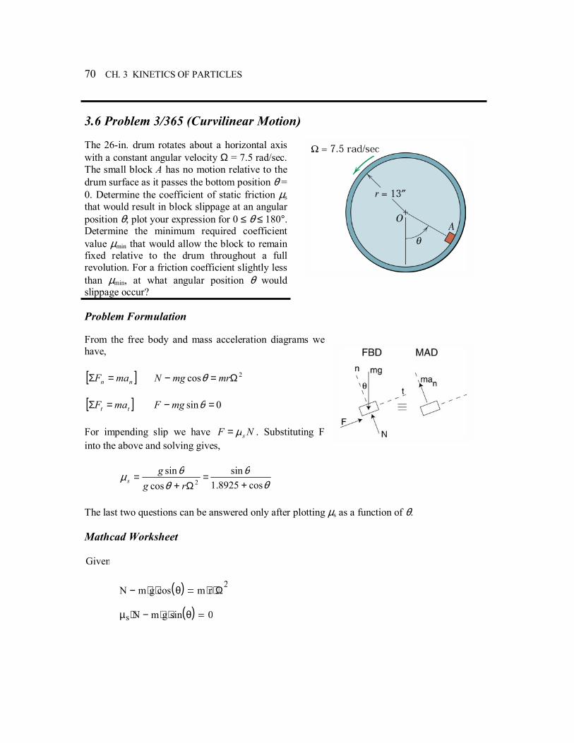
3.6 Problem 3/365 (Curvilinear Motion) The 26-in. drum rotates about a horizontal axis with a constant angular velocity Ω = 7.5 rad/sec. The small block A has no motion relative to the drum surface as it passes the bottom position θ = 0. Determine the coefficient of static friction µs that would result in block slippage at an angular position θ; plot your expression for 0 ≤ θ ≤ 180°. Determine the minimum required coefficient value µmin that would allow the block to remain fixed relative to the drum throughout a full revolution. For a friction coefficient slightly less than µmin, at what angular position θ would slippage occur? Problem Formulation From the free body and mass acceleration diagrams we have, [ ]nn maF =Σ 2cos Ω=− mrmgN θ [ ]tt maF =Σ 0sin =− θmgF For impending slip we have NF sµ= . Substituting F into the above and solving gives,
θ
θθ
θµcos8925.1
sincos
sin2 +
=Ω+
=rg
gs
The last two questions can be answered only after plotting µs as a function of θ. Mathcad Worksheet Given
N m g⋅ cos θ( )⋅− m r⋅ Ω2
⋅ µs N⋅ m g⋅ sin θ( )⋅− 0
KINETICS OF PARTICLES 71
Find µs N,( )g
sin θ( )g cos θ( )⋅ r Ω
2⋅+( )⋅
m g⋅ cos θ( )⋅ m r⋅ Ω2
⋅+
→
g 32.2:= r1312
:= Ω 7.5:=
µs θ( ) gsin θ( )
g cos θ( )⋅ r Ω2
⋅+( )⋅:=
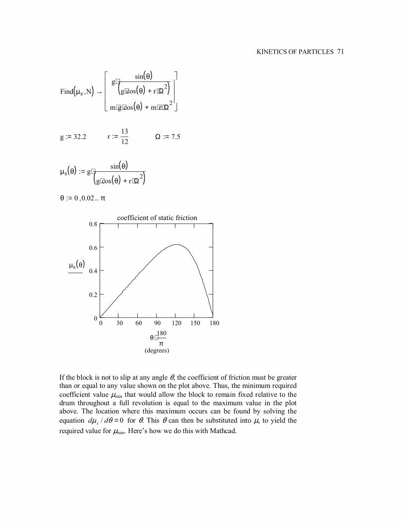
θ 0 0.02, π..:=
0 30 60 90 120 150 1800
0.2
0.4
0.6
0.8coefficient of static friction
(degrees)
µs θ( )
θ180π
⋅
If the block is not to slip at any angle θ, the coefficient of friction must be greater than or equal to any value shown on the plot above. Thus, the minimum required coefficient value µmin that would allow the block to remain fixed relative to the drum throughout a full revolution is equal to the maximum value in the plot above. The location where this maximum occurs can be found by solving the equation 0/ =θµ dd s for θ. This θ can then be substituted into µs to yield the required value for µmin. Heres how we do this with Mathcad.
72 CH. 3 KINETICS OF PARTICLES
xµs x( )d
d0 solve x,
2.1275232852017454951−
2.1275232852017454951
→ µs 2.1275( ) 0.622= From the above we see that µmin = 0.622. If µs is slightly less than this value, the block will slip when θ = 2.128 rads (121.9°).
KINETICS OF SYSTEMS OF PARTICLES This chapter concerns the extension of principles covered in chapters two and three to the study of the motion of general systems of particles. The chapter first considers the three approaches introduced in chapter 3 (direct application of Newtons second law, work/energy, and impulse/momentum) and then moves to other applications such as steady mass flow and variable mass. Problem 4.1 considers an application of the conservation of momentum to a system comprised of a small car and an attached rotating sphere. Mathcad is used to plot the velocity of the car as a function of the angular position of the sphere. The absolute position of the sphere is also plotted. Problem 4.2 uses the concept of steady mass flow to study the effects of geometry upon the design of a sprinkler system. One of the main purposes of this problem is to illustrate how a problem can be greatly simplified using non-dimensional analysis. In particular, an equation containing seven parameters is reduced to a non-dimensional equation with only three parameters. Problem 4.3 is a variable mass problem in which Mathcad is used to integrate the kinematic equation adxvdv = . Symbolic solve and simplify are also illustrated.
4
74 CH. 4 KINETICS OF SYSTEMS OF PARTICLES
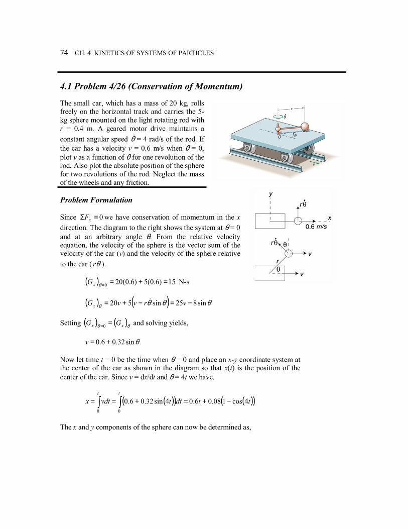
4.1 Problem 4/26 (Conservation of Momentum) The small car, which has a mass of 20 kg, rolls freely on the horizontal track and carries the 5-kg sphere mounted on the light rotating rod with r = 0.4 m. A geared motor drive maintains a constant angular speed θ& = 4 rad/s of the rod. If the car has a velocity v = 0.6 m/s when θ = 0, plot v as a function of θ for one revolution of the rod. Also plot the absolute position of the sphere for two revolutions of the rod. Neglect the mass of the wheels and any friction. Problem Formulation Since 0=Σ xF we have conservation of momentum in the x direction. The diagram to the right shows the system at θ = 0 and at an arbitrary angle θ. From the relative velocity equation, the velocity of the sphere is the vector sum of the velocity of the car (v) and the velocity of the sphere relative to the car ( θ&r ). ( ) 15)6.0(5)6.0(200 =+==θxG N•s ( ) ( ) θθθθ sin825sin520 −=−+= vrvvGx
& Setting ( ) ( )θθ xx GG ==0 and solving yields, θsin32.06.0 +=v Now let time t = 0 be the time when θ = 0 and place an x-y coordinate system at the center of the car as shown in the diagram so that x(t) is the position of the center of the car. Since v = dx/dt and θ = 4t we have,
( )( ) ( )( )∫ ∫ −+=+==t t
ttdttvdtx0 0
4cos108.06.04sin32.06.0
The x and y components of the sphere can now be determined as,
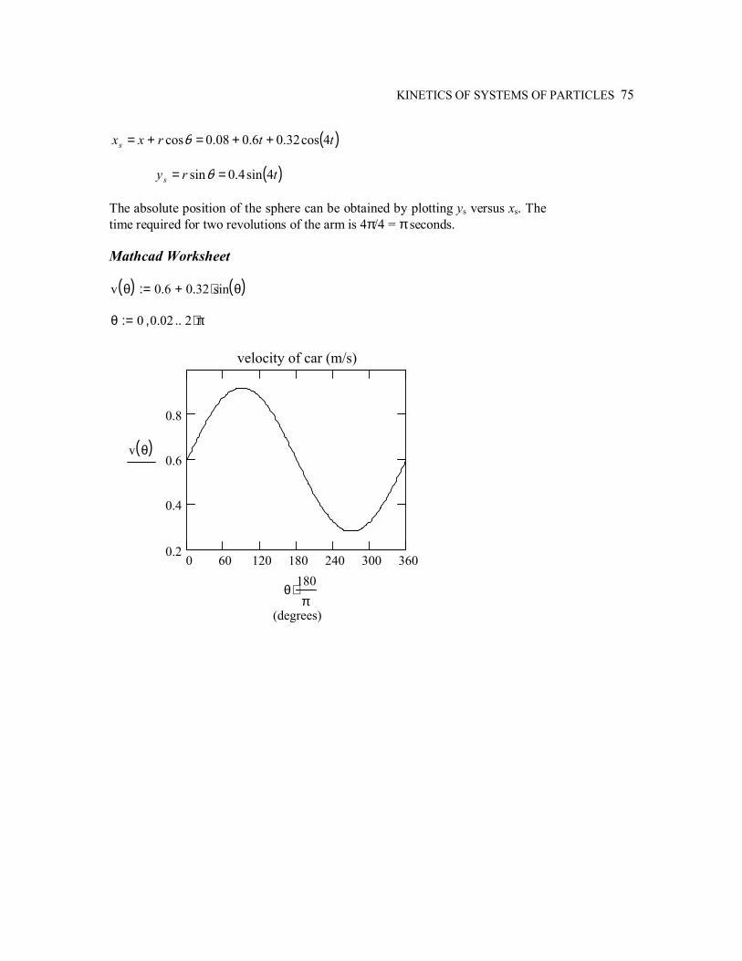
KINETICS OF SYSTEMS OF PARTICLES 75
( )ttrxxs 4cos32.06.008.0cos ++=+= θ ( )trys 4sin4.0sin == θ The absolute position of the sphere can be obtained by plotting ys versus xs. The time required for two revolutions of the arm is 4π/4 = π seconds. Mathcad Worksheet v θ( ) 0.6 0.32 sin θ( )⋅+:= θ 0 0.02, 2 π⋅..:=
0 60 120 180 240 300 3600.2
0.4
0.6
0.8
velocity of car (m/s)
(degrees)
v θ( )
θ180π
⋅
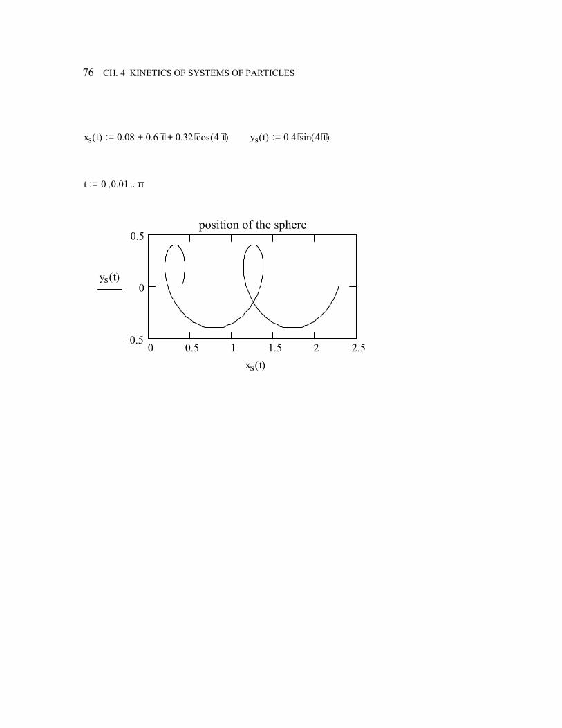
76 CH. 4 KINETICS OF SYSTEMS OF PARTICLES
xs t( ) 0.08 0.6 t⋅+ 0.32 cos 4 t⋅( )⋅+:= ys t( ) 0.4 sin 4 t⋅( )⋅:= t 0 0.01, π..:=
0 0.5 1 1.5 2 2.50.5
0
0.5position of the sphere
ys t( )
xs t( )
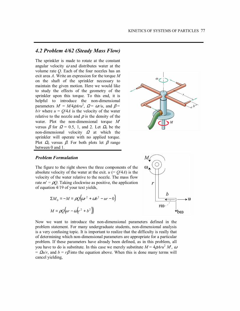
KINETICS OF SYSTEMS OF PARTICLES 77
4.2 Problem 4/62 (Steady Mass Flow) The sprinkler is made to rotate at the constant angular velocity ω and distributes water at the volume rate Q. Each of the four nozzles has an exit area A. Write an expression for the torque M on the shaft of the sprinkler necessary to maintain the given motion. Here we would like to study the effects of the geometry of the sprinkler upon this torque. To this end, it is helpful to introduce the non-dimensional parameters M′ = M/4ρAru2, Ω = ωr/u, and β = b/r where u = Q/4A is the velocity of the water relative to the nozzle and ρ is the density of the water. Plot the non-dimensional torque M′ versus β for Ω = 0.5, 1, and 2. Let Ω0 be the non-dimensional velocity Ω at which the sprinkler will operate with no applied torque. Plot Ω0 versus β. For both plots let β range between 0 and 1. Problem Formulation The figure to the right shows the three components of the absolute velocity of the water at the exit. u (= Q/4A) is the velocity of the water relative to the nozzle. The mass flow rate m′ = ρQ. Taking clockwise as positive, the application of equation 4/19 of your text yields,
( )0220 −−+=−=Σ urbrQMM ωωρ
( )( )22 brurQM +−= ωρ Now we want to introduce the non-dimensional parameters defined in the problem statement. For many undergraduate students, non-dimensional analysis is a very confusing topic. It is important to realize that the difficulty is really that of determining which non-dimensional parameters are appropriate for a particular problem. If these parameters have already been defined, as in this problem, all you have to do is substitute. In this case we merely substitute M = 4ρAru2 M′, ω = Ωu/r, and b = rβ into the equation above. When this is done many terms will cancel yielding,
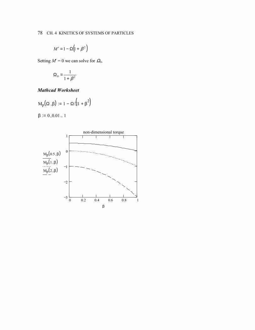
78 CH. 4 KINETICS OF SYSTEMS OF PARTICLES
( )211 β+Ω−=′M Setting M′ = 0 we can solve for Ω0,
20 11β+
=Ω
Mathcad Worksheet
Mp Ω β,( ) 1 Ω 1 β2
+( )⋅−:= β 0 0.01, 1..:=
0 0.2 0.4 0.6 0.8 13
2
1
0
1non-dimensional torque
Mp 0.5 β,( )
Mp 1 β,( )
Mp 2 β,( )
β
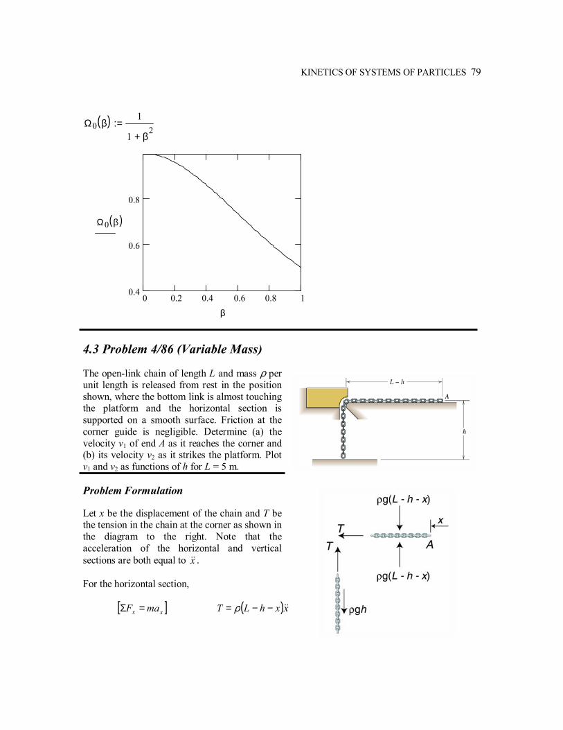
KINETICS OF SYSTEMS OF PARTICLES 79
Ω0 β( ) 1
1 β2
+:=
0 0.2 0.4 0.6 0.8 10.4
0.6
0.8
Ω0 β( )
β
4.3 Problem 4/86 (Variable Mass) The open-link chain of length L and mass ρ per unit length is released from rest in the position shown, where the bottom link is almost touching the platform and the horizontal section is supported on a smooth surface. Friction at the corner guide is negligible. Determine (a) the velocity v1 of end A as it reaches the corner and (b) its velocity v2 as it strikes the platform. Plot v1 and v2 as functions of h for L = 5 m. Problem Formulation Let x be the displacement of the chain and T be the tension in the chain at the corner as shown in the diagram to the right. Note that the acceleration of the horizontal and vertical sections are both equal to x&& . For the horizontal section,
[ ]xx maF =Σ ( )xxhLT &&−−= ρ
80 CH. 4 KINETICS OF SYSTEMS OF PARTICLES
For the vertical section,
[ ]yy maF =Σ↓ xhTgh &&ρρ =− Substituting T from the first equation into the second and simplifying gives,
xL
ghx−
=&&
Now we use the relation adxvdv = to write,
dxxL
ghvdv
hLv
∫∫−
−=
00
1
=
−= ∫
−
hLghdx
xLghv
hL
ln220
21
( )hLghv /ln21 = After end A has passed the corner it will be in free-fall until it hits the platform. With y positive down we have vdv = gdy yielding,
( ) ghvv =− 21
222
1
Substituting for v1 and solving, ( ))/ln(122 hLghv += Mathcad Worksheet
First we solve the equation ( )∫∫−
−=hLv
dxxLghvdv00
/1
for v1.
eqn10
v1vv
⌠⌡
d
0
L h−
xg h⋅
L x−
⌠⌡
d:=h
KINETICS OF SYSTEMS OF PARTICLES 81
eqn1solve v1,
simplify
2− g⋅ h⋅ ln h( ) ln L( )−( )⋅[ ]
12
2− g− h⋅ ln h( ) ln L( )−( )⋅[ ]
12⋅
→
Mathcad has found two solutions. The first is the one we want since it is positive. This solution can easily be simplified to the result given above in the problem formulation section. Once v1 is known it is rather easy to find v2. Well do it symbolically here for purposes of illustration. First we copy and paste the first solution above to define v1. Then we solve the
equation ∫∫ ==hv
vghgdyvdv
0
2
1
for v2. Note how the result for v1 is automatically
substituted.
v1 2 g h⋅ ln h( )− ln L( )+( )⋅[ ]
12⋅:= h
eqn2v1
v2vv
⌠⌡
d g h⋅:= h
eqn2solve v2,
simplify
2 g h⋅ ln h( )− ln L( )+ 1+( )⋅[ ]
12⋅
2− g h⋅ ln h( )− ln L( )+ 1+( )⋅[ ]
12⋅
→
Once again, the first solution will simplify to that given in the problem formulation section above. L 5:=
v1 h( ) 2 g h⋅ ln h( )− ln L( )+( )⋅[ ]
12⋅:=
v2 h( ) 2 g h⋅ ln h( )− ln L( )+ 1+( )⋅[ ]
12⋅:=
h 0 0.01, L..:=
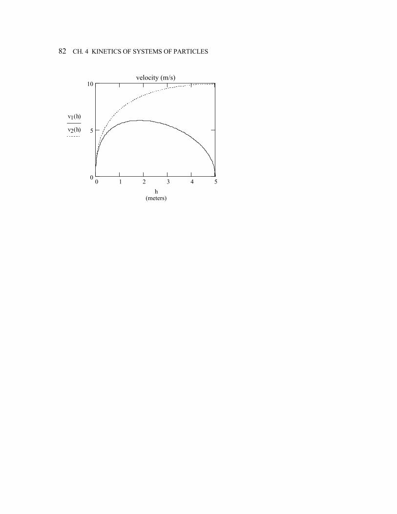
82 CH. 4 KINETICS OF SYSTEMS OF PARTICLES
0 1 2 3 4 50
5
10velocity (m/s)
(meters)
v1 h( )
v2 h( )
h
PLANE KINEMATICS OF RIGID BODIES This chapter extends the kinematic analysis of particles covered in chapter 2 to rigid bodies by taking into account the rotational motion of the body. Thus, the motion of rigid bodies involves both translation and rotation. Problem 5.1 is a straightforward problem comparing angular displacement with the total number of revolutions. The problem also illustrates symbolic integration. Problem 5.2 is an interesting application of absolute motion analysis. Illustrated in this problem are the simultaneous (symbolic) solution of multiple equations and differentiation with respect to time of a function whose explicit time dependence is not known. In problem 5.3 the velocity of the piston in a reciprocating engine is plotted versus the angular orientation of the crank. The maximum velocity and the corresponding orientation (of the crank) are then obtained. The orientation at which the maximum occurs is found by solving the equation dv/dθ = 0. This is a rare case where both symbolic solve and GivenFind fail to find a solution. Thus, root is used to obtain a numerical solution. The instantaneous center of zero velocity is used in problem 5.4 to relate the velocity of a vertical control rod to the angular velocity of a rotating bar in a switching device. Problem 5.5 is a fairly straightforward relative acceleration problem while problem 5.6 considers the reciprocating engine of problem 5.3 but uses absolute rather than relative motion analysis. The problem illustrates the use of computer algebra for carrying out some tedious calculations including differentiation and substitution.
5
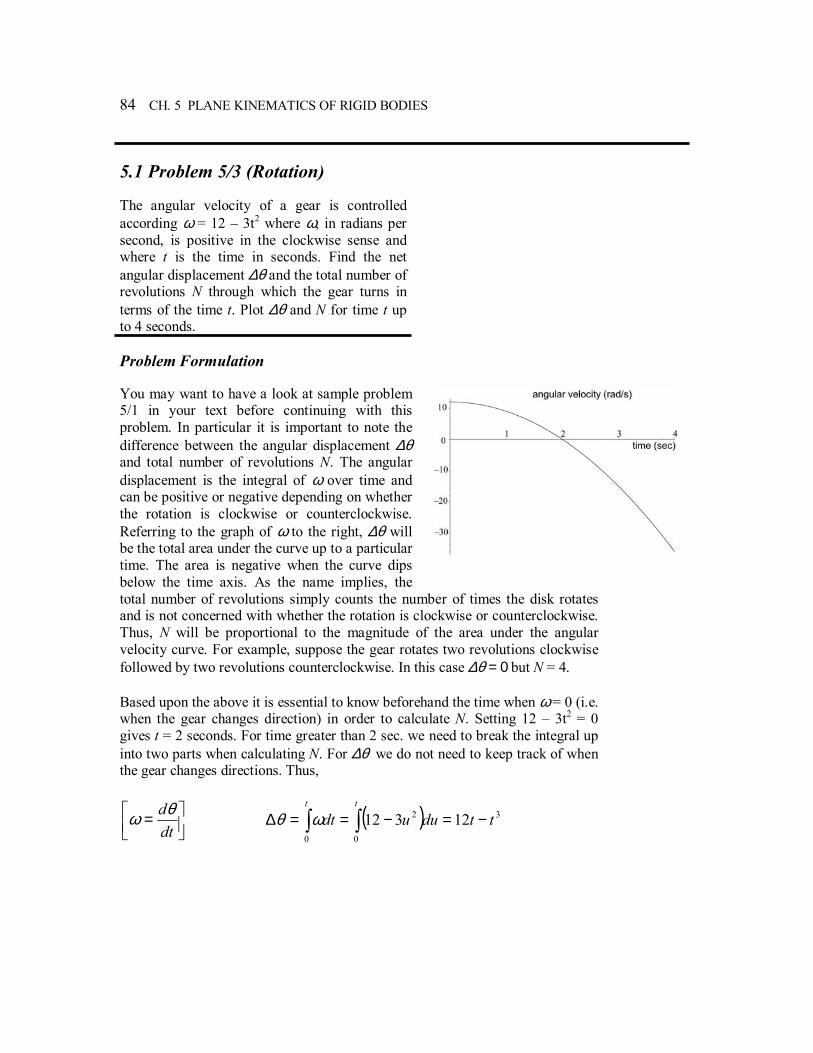
84 CH. 5 PLANE KINEMATICS OF RIGID BODIES
5.1 Problem 5/3 (Rotation) The angular velocity of a gear is controlled according ω = 12 3t2 where ω, in radians per second, is positive in the clockwise sense and where t is the time in seconds. Find the net angular displacement ∆θ and the total number of revolutions N through which the gear turns in terms of the time t. Plot ∆θ and N for time t up to 4 seconds. Problem Formulation You may want to have a look at sample problem 5/1 in your text before continuing with this problem. In particular it is important to note the difference between the angular displacement ∆θ and total number of revolutions N. The angular displacement is the integral of ω over time and can be positive or negative depending on whether the rotation is clockwise or counterclockwise. Referring to the graph of ω to the right, ∆θ will be the total area under the curve up to a particular time. The area is negative when the curve dips below the time axis. As the name implies, the total number of revolutions simply counts the number of times the disk rotates and is not concerned with whether the rotation is clockwise or counterclockwise. Thus, N will be proportional to the magnitude of the area under the angular velocity curve. For example, suppose the gear rotates two revolutions clockwise followed by two revolutions counterclockwise. In this case ∆θ = 0 but N = 4. Based upon the above it is essential to know beforehand the time when ω = 0 (i.e. when the gear changes direction) in order to calculate N. Setting 12 3t2 = 0 gives t = 2 seconds. For time greater than 2 sec. we need to break the integral up into two parts when calculating N. For ∆θ we do not need to keep track of when the gear changes directions. Thus,
=
dtdθω ( ) 3
0 0
2 12312 ttduudtt t
−=−==∆ ∫ ∫ωθ
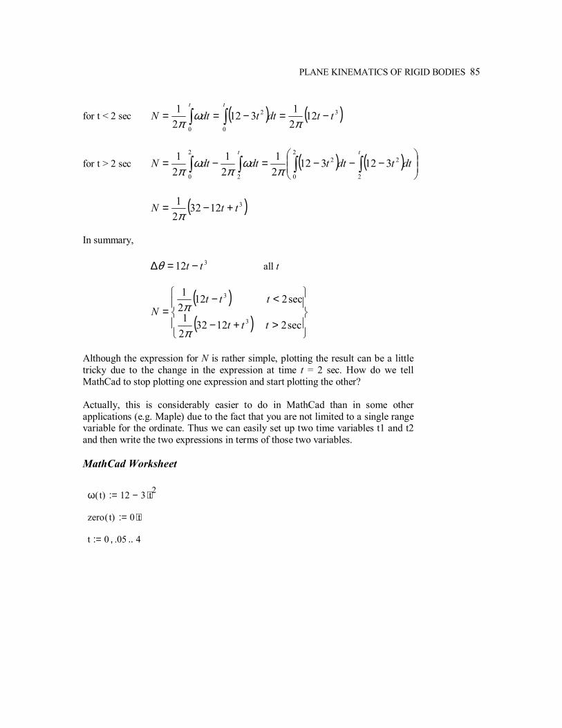
PLANE KINEMATICS OF RIGID BODIES 85
for t < 2 sec ( ) ( )3
0 0
2 1221312
21 ttdttdtN
t t
−=−== ∫ ∫ πω
π
for t > 2 sec ( ) ( )
−−−=−= ∫∫∫ ∫ dttdttdtdtN
tt
2
22
0
22
0 2
31231221
21
21
πω
πω
π
( )3123221 ttN +−=π
In summary,
312 tt −=∆θ all t
( )( )
>+−
<−=
sec2123221
sec21221
3
3
ttt
tttN
π
π
Although the expression for N is rather simple, plotting the result can be a little tricky due to the change in the expression at time t = 2 sec. How do we tell MathCad to stop plotting one expression and start plotting the other? Actually, this is considerably easier to do in MathCad than in some other applications (e.g. Maple) due to the fact that you are not limited to a single range variable for the ordinate. Thus we can easily set up two time variables t1 and t2 and then write the two expressions in terms of those two variables. MathCad Worksheet
ω t( ) 12 3 t2⋅−:=
zero t( ) 0 t⋅:=
t 0 .05, 4..:=
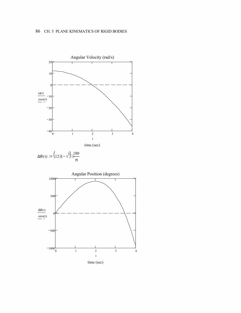
86 CH. 5 PLANE KINEMATICS OF RIGID BODIES
0 1 2 3 440
30
20
10
0
10
20Angular Velocity (rad/s)
time (sec)
ω t( )
zero t( )
t
∆θ t( ) 12 t⋅ t3−( ) 180π
⋅:=
0 1 2 3 41000
500
0
500
1000Angular Position (degrees)
time (sec)
∆θ t( )
zero t( )
t
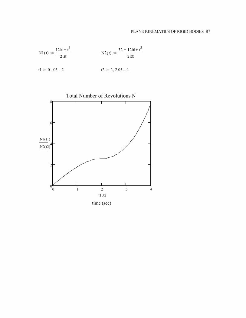
PLANE KINEMATICS OF RIGID BODIES 87
N1 t( )12 t⋅ t3−
2 π⋅:= N2 t( )
32 12 t⋅− t3+2 π⋅
:=
t1 0 .05, 2..:= t2 2 2.05, 4..:=
0 1 2 3 40
2
4
6
8Total Number of Revolutions N
time (sec)
N1 t1( )
N2 t2( )
t1 t2,
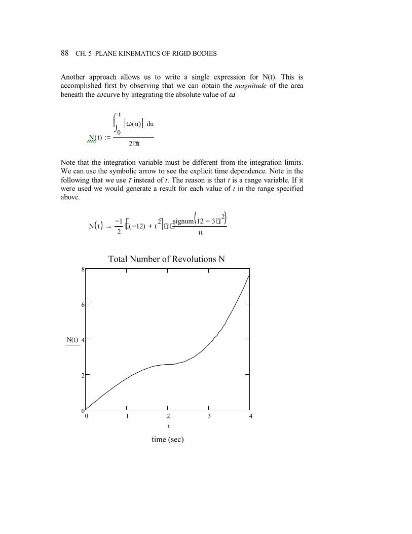
88 CH. 5 PLANE KINEMATICS OF RIGID BODIES
Another approach allows us to write a single expression for N(t). This is accomplished first by observing that we can obtain the magnitude of the area beneath the ω curve by integrating the absolute value of ω.
N t( )0
tuω u( )
⌠⌡
d
2 π⋅:=
Note that the integration variable must be different from the integration limits. We can use the symbolic arrow to see the explicit time dependence. Note in the following that we use τ instead of t. The reason is that t is a range variable. If it were used we would generate a result for each value of t in the range specified above.
N τ( ) 1−
212−( ) τ2+ τ
signum 12 3 τ2⋅−( )π
⋅⋅⋅→
0 1 2 3 40
2
4
6
8Total Number of Revolutions N
time (sec)
N t( )
t
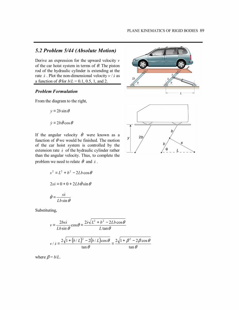
PLANE KINEMATICS OF RIGID BODIES 89
5.2 Problem 5/44 (Absolute Motion) Derive an expression for the upward velocity v of the car hoist system in terms of θ. The piston rod of the hydraulic cylinder is extending at the rate s& . Plot the non-dimensional velocity v / s& as a function of θ for b/L = 0.1, 0.5, 1, and 2. Problem Formulation From the diagram to the right, θsin2by = θθ cos2 && by = If the angular velocity θ& were known as a function of θ we would be finished. The motion of the car hoist system is controlled by the extension rate s& of the hydraulic cylinder rather than the angular velocity. Thus, to complete the problem we need to relate θ& and s& . θcos2222 LbbLs −+= θθ sin2002 && Lbss ++=
θ
θsinLbss&& =
Substituting,
θ
θθθ tan
cos22cossin
2 22
LLbbLs
Lbsbsv −+==
&&
( ) ( )
θθββ
θθ
tancos212
tancos/2/12
/22 −+
=−+
=LbLb
sv &
where β = b/L.
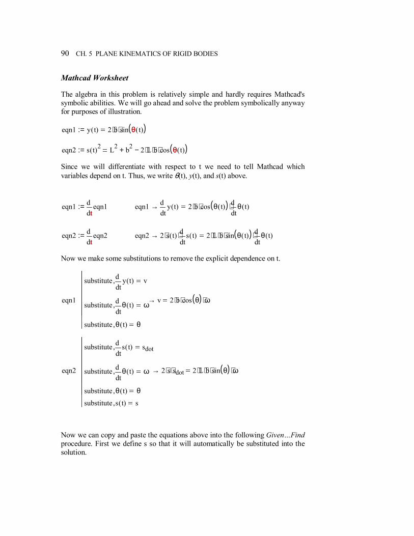
90 CH. 5 PLANE KINEMATICS OF RIGID BODIES
Mathcad Worksheet The algebra in this problem is relatively simple and hardly requires Mathcad's symbolic abilities. We will go ahead and solve the problem symbolically anyway for purposes of illustration. eqn1 y t( ) 2 b⋅ sin θ t( )( )⋅:= θ
eqn2 s t( )2 L2 b2+ 2 L⋅ b⋅ cos θ t( )( )⋅−:= θ Since we will differentiate with respect to t we need to tell Mathcad which variables depend on t. Thus, we write θ(t), y(t), and s(t) above.
eqn1teqn1d
d:=
t eqn1
ty t( )d
d2 b⋅ cos θ t( )( )⋅
tθ t( )d
d⋅→
eqn2teqn2d
d:=
t eqn2 2 s t( )⋅
ts t( )d
d⋅ 2 L⋅ b⋅ sin θ t( )( )⋅
tθ t( )d
d⋅→
Now we make some substitutions to remove the explicit dependence on t.
eqn1
substitutety t( )d
dv,
substitutetθ t( )d
dω,
substitute θ t( ) θ,
v 2 b⋅ cos θ( )⋅ ω⋅→
eqn2
substitutets t( )d
dsdot,
substitutetθ t( )d
dω,
substitute θ t( ) θ,
substitute s t( ) s,
2 s⋅ sdot⋅ 2 L⋅ b⋅ sin θ( )⋅ ω⋅→
Now we can copy and paste the equations above into the following GivenFind procedure. First we define s so that it will automatically be substituted into the solution.
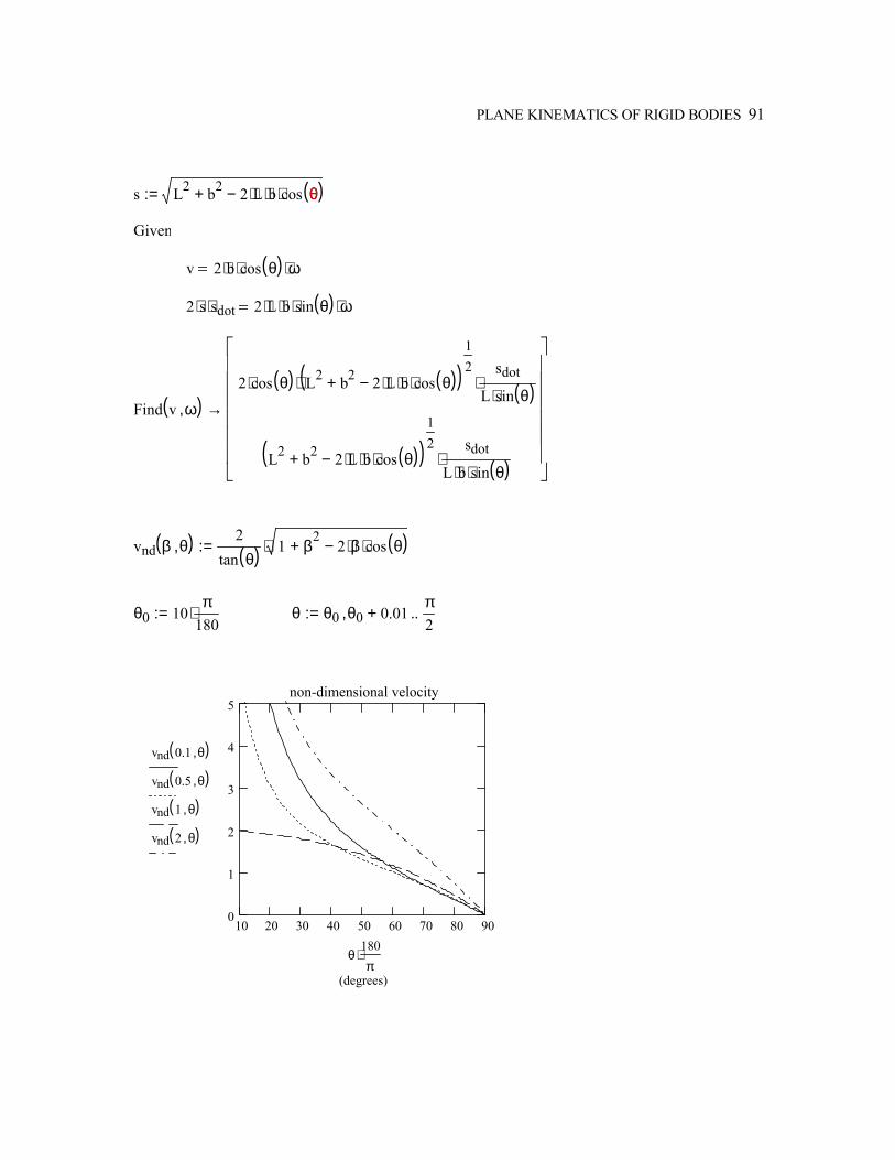
PLANE KINEMATICS OF RIGID BODIES 91
s L2 b2+ 2 L⋅ b⋅ cos θ( )⋅−:= θ Given
v 2 b⋅ cos θ( )⋅ ω⋅ 2 s⋅ sdot⋅ 2 L⋅ b⋅ sin θ( )⋅ ω⋅
Find v ω,( )2 cos θ( )⋅ L2 b2 2 L⋅ b⋅ cos θ( )⋅−+( )
12
⋅sdot
L sin θ( )⋅⋅
L2 b2 2 L⋅ b⋅ cos θ( )⋅−+( )12 sdot
L b sin θ( )⋅⋅⋅
→
vnd β θ,( ) 2tan θ( ) 1 β
2+ 2 β⋅ cos θ( )⋅−⋅:=
θ0 10π
180⋅:= θ θ0 θ0 0.01+,
π2
..:=
10 20 30 40 50 60 70 80 900
1
2
3
4
5non-dimensional velocity
(degrees)
vnd 0.1 θ,( )
vnd 0.5 θ,( )
vnd 1 θ,( )
vnd 2 θ,( )
θ180π
⋅
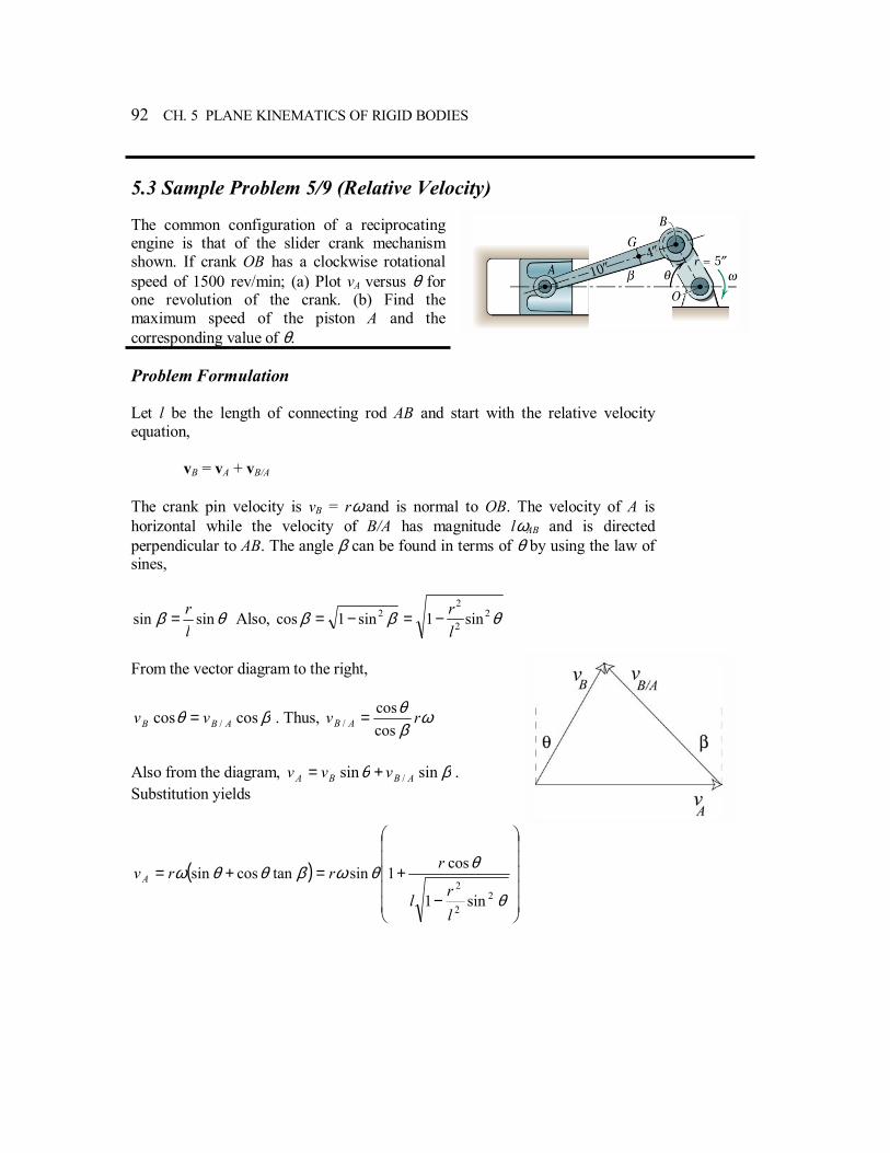
92 CH. 5 PLANE KINEMATICS OF RIGID BODIES
5.3 Sample Problem 5/9 (Relative Velocity) The common configuration of a reciprocating engine is that of the slider crank mechanism shown. If crank OB has a clockwise rotational speed of 1500 rev/min; (a) Plot vA versus θ for one revolution of the crank. (b) Find the maximum speed of the piston A and the corresponding value of θ. Problem Formulation Let l be the length of connecting rod AB and start with the relative velocity equation, vB = vA + vB/A The crank pin velocity is vB = rω and is normal to OB. The velocity of A is horizontal while the velocity of B/A has magnitude lωAB and is directed perpendicular to AB. The angle β can be found in terms of θ by using the law of sines,
θβ sinsinlr= Also, θββ 2
2
22 sin1sin1cos
lr−=−=
From the vector diagram to the right,
βθ coscos / ABB vv = . Thus, ωβθ rv AB cos
cos/ =
Also from the diagram, βθ sinsin / ABBA vvv += . Substitution yields
( )
−
+=+=
θ
θθωβθθω2
2
2
sin1
cos1sintancossin
lrl
rrrvA
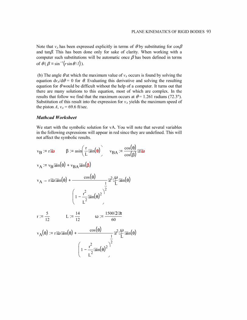
PLANE KINEMATICS OF RIGID BODIES 93
Note that vA has been expressed explicitly in terms of θ by substituting for cosβ and tanβ. This has been done only for sake of clarity. When working with a computer such substitutions will be automatic once β has been defined in terms of θ ( ( )lr /sinsin 1 θβ −= ). (b) The angle θ at which the maximum value of vA occurs is found by solving the equation dvA/dθ = 0 for θ. Evaluating this derivative and solving the resulting equation for θ would be difficult without the help of a computer. It turns out that there are many solutions to this equation, most of which are complex. In the results that follow we find that the maximum occurs at θ = 1.261 radians (72.3°). Substitution of this result into the expression for vA yields the maximum speed of the piston A, vA = 69.6 ft/sec. Mathcad Worksheet We start with the symbolic solution for vA. You will note that several variables in the following expressions will appear in red since they are undefined. This will not affect the symbolic results.
vB r ω⋅:= ω β asinrL
sin θ( )⋅
:= θ vBAcos θ( )cos β( ) r⋅ ω⋅:= ω
vA vB sin θ( )⋅ vBA sin β( )⋅+:= β
vA r ω⋅ sin θ( )⋅cos θ( )
1r2
L2sin θ( )2
⋅−
12
r2⋅ωL
⋅ sin θ( )⋅+→
r512
:= L1412
:= ω1500 2⋅ π⋅
60:=
vA θ( ) r ω⋅ sin θ( )⋅cos θ( )
1r2
L2sin θ( )2
⋅−
12
r2⋅ωL
⋅ sin θ( )⋅+:=
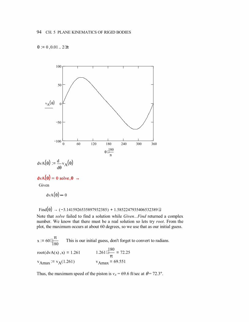
94 CH. 5 PLANE KINEMATICS OF RIGID BODIES
θ 0 0.01, 2 π⋅..:=
0 60 120 180 240 300 360100
50
0
50
100
vA θ( )
θ180π
⋅
dvA θ( )θ
vA θ( )dd
:=
dvA θ( ) 0 solve θ, →dvA θ( ) 0 solve θ, →
Given
dvA θ( ) 0
Find θ( ) 3.1415926535897932385−( ) 1.5852247935406532389 i⋅+→ Note that solve failed to find a solution while Given...Find returned a complex number. We know that there must be a real solution so lets try root. From the plot, the maximum occurs at about 60 degrees, so we use that as our initial guess.
x 60π
180⋅:= This is our initial guess, don't forget to convert to radians.
root dvA x( ) x,( ) 1.261= 1.261180π
⋅ 72.25=
vAmax vA 1.261( ):= vAmax 69.551=
Thus, the maximum speed of the piston is vA = 69.6 ft/sec at θ = 72.3°.
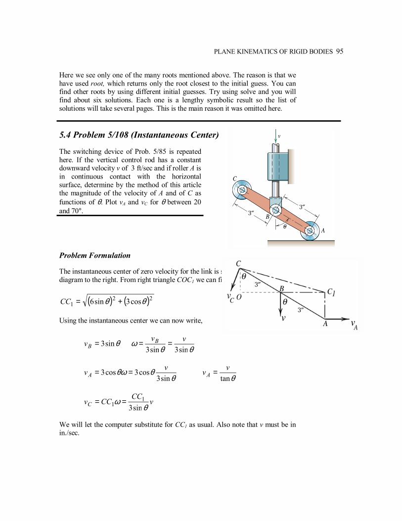
PLANE KINEMATICS OF RIGID BODIES 95
Here we see only one of the many roots mentioned above. The reason is that we have used root, which returns only the root closest to the initial guess. You can find other roots by using different initial guesses. Try using solve and you will find about six solutions. Each one is a lengthy symbolic result so the list of solutions will take several pages. This is the main reason it was omitted here. 5.4 Problem 5/108 (Instantaneous Center) The switching device of Prob. 5/85 is repeated here. If the vertical control rod has a constant downward velocity v of 3 ft/sec and if roller A is in continuous contact with the horizontal surface, determine by the method of this article the magnitude of the velocity of A and of C as functions of θ. Plot vA and vC for θ between 20 and 70°. Problem Formulation The instantaneous center of zero velocity for the link is shown (point C1) in the diagram to the right. From right triangle COC1 we can find the length CC1 as
( ) ( )221 cos3sin6 θθ +=CC
Using the instantaneous center we can now write,
θsin3=Bv θθ
ωsin3sin3vvB ==
θ
θθωsin3
cos3cos3 vvA == θtan
vvA =
vCC
CCvC θω
sin31
1 ==
We will let the computer substitute for CC1 as usual. Also note that v must be in in./sec.
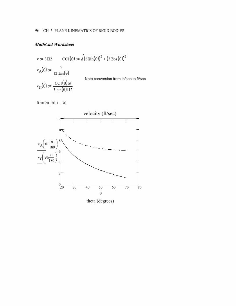
96 CH. 5 PLANE KINEMATICS OF RIGID BODIES
MathCad Worksheet
v 3 12⋅:= CC1 θ( ) 6 sin θ( )⋅( )2 3 cos θ( )⋅( )2+:=
vA θ( ) v12 tan θ( )⋅
:=
Note conversion from in/sec to ft/sec
vC θ( ) CC1 θ( ) v⋅3 sin θ( )⋅ 12⋅
:=
θ 20 20.1, 70..:=
20 30 40 50 60 70 800
2
4
6
8
10
12velocity (ft/sec)
theta (degrees)
vA θπ
180⋅
vC θπ
180⋅
θ
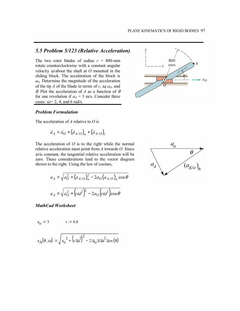
PLANE KINEMATICS OF RIGID BODIES 97
5.5 Problem 5/123 (Relative Acceleration) The two rotor blades of radius r = 800-mm rotate counterclockwise with a constant angular velocity ω about the shaft at O mounted in the sliding block. The acceleration of the block is aO. Determine the magnitude of the acceleration of the tip A of the blade in terms of r, ω, aO, and θ. Plot the acceleration of A as a function of θ for one revolution if aO = 3 m/s. Consider three cases: ω = 2, 4, and 6 rad/s. Problem Formulation The acceleration of A relative to O is
( ) ( )tOAnOAOA aaaa //rrrr ++=
The acceleration of O is to the right while the normal relative acceleration must point from A towards O. Since ω is constant, the tangential relative acceleration will be zero. These considerations lead to the vector diagram shown to the right. Using the law of cosines,
( ) ( ) θcos2 /2
/2
nOAOnOAOA aaaaa −+=
( ) ( ) θωω cos2 2222 raraa OOA −+=
MathCad Worksheet
ao 3:= r 0.8:=
aA θ ω,( ) ao2 r ω2⋅( )2
+ 2 ao⋅ r⋅ ω2⋅ cos θ( )⋅−:=
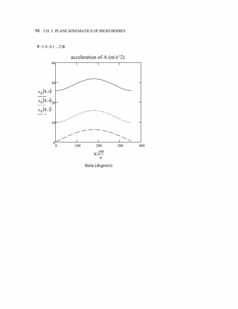
98 CH. 5 PLANE KINEMATICS OF RIGID BODIES
θ 0 0.1, 2 π⋅..:=
0 100 200 300 4000
10
20
30
40acceleration of A (m/s^2)
theta (degrees)
aA θ 6,( )
aA θ 4,( )
aA θ 2,( )
θ180π
⋅
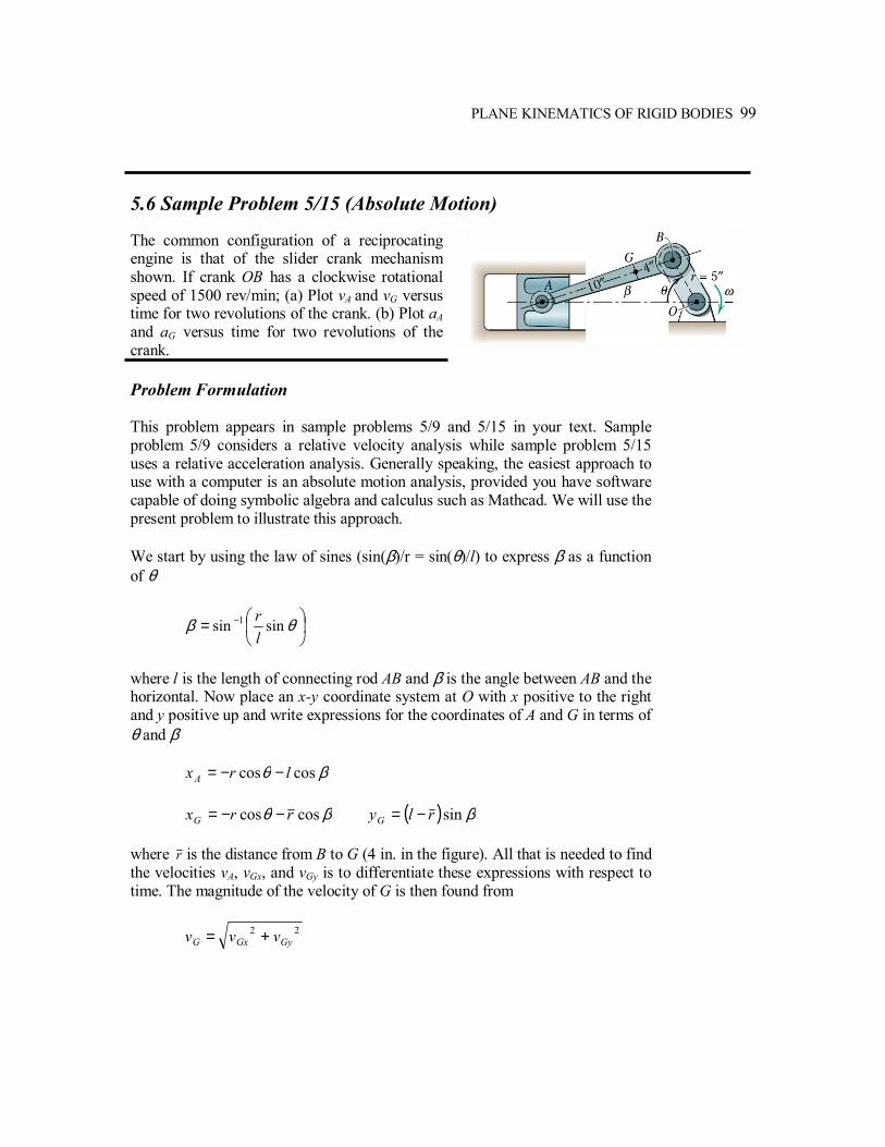
PLANE KINEMATICS OF RIGID BODIES 99
5.6 Sample Problem 5/15 (Absolute Motion) The common configuration of a reciprocating engine is that of the slider crank mechanism shown. If crank OB has a clockwise rotational speed of 1500 rev/min; (a) Plot vA and vG versus time for two revolutions of the crank. (b) Plot aA and aG versus time for two revolutions of the crank. Problem Formulation This problem appears in sample problems 5/9 and 5/15 in your text. Sample problem 5/9 considers a relative velocity analysis while sample problem 5/15 uses a relative acceleration analysis. Generally speaking, the easiest approach to use with a computer is an absolute motion analysis, provided you have software capable of doing symbolic algebra and calculus such as Mathcad. We will use the present problem to illustrate this approach. We start by using the law of sines (sin(β)/r = sin(θ)/l) to express β as a function of θ
= − θβ sinsin 1
lr
where l is the length of connecting rod AB and β is the angle between AB and the horizontal. Now place an x-y coordinate system at O with x positive to the right and y positive up and write expressions for the coordinates of A and G in terms of θ and β βθ coscos lrxA −−= βθ coscos rrxG −−= ( ) βsinrlyG −=
where r is the distance from B to G (4 in. in the figure). All that is needed to find the velocities vA, vGx, and vGy is to differentiate these expressions with respect to time. The magnitude of the velocity of G is then found from
22GyGxG vvv +=
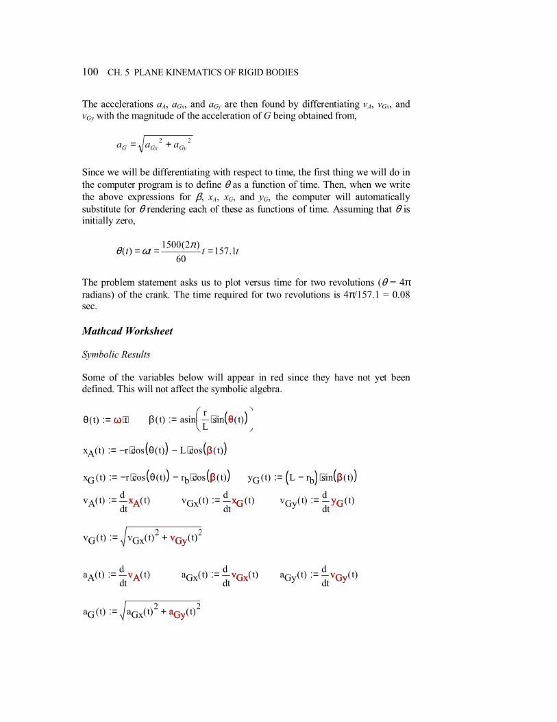
100 CH. 5 PLANE KINEMATICS OF RIGID BODIES
The accelerations aA, aGx, and aGy are then found by differentiating vA, vGx, and vGy with the magnitude of the acceleration of G being obtained from,
22GyGxG aaa +=
Since we will be differentiating with respect to time, the first thing we will do in the computer program is to define θ as a function of time. Then, when we write the above expressions for β, xA, xG, and yG, the computer will automatically substitute for θ rendering each of these as functions of time. Assuming that θ is initially zero,
tttt 1.15760
)2(1500)( === πωθ
The problem statement asks us to plot versus time for two revolutions (θ = 4π radians) of the crank. The time required for two revolutions is 4π/157.1 = 0.08 sec. Mathcad Worksheet Symbolic Results Some of the variables below will appear in red since they have not yet been defined. This will not affect the symbolic algebra.
θ t( ) ω t⋅:= ω β t( ) asinrL
sin θ t( )( )⋅
:= θ
xA t( ) r− cos θ t( )( )⋅ L cos β t( )( )⋅−:= β xG t( ) r− cos θ t( )( )⋅ rb cos β t( )( )⋅−:= β yG t( ) L rb−( ) sin β t( )( )⋅:= β
vA t( )txA t( )d
d:= xA vGx t( )
txG t( )d
d:= xG vGy t( )
tyG t( )d
d:= yG
vG t( ) vGx t( )2 vGy t( )2+:= vGy
aA t( )tvA t( )d
d:= vA aGx t( )
tvGx t( )d
d:= vGx aGy t( )
tvGy t( )d
d:= vGy
aG t( ) aGx t( )2 aGy t( )2+:= aGy
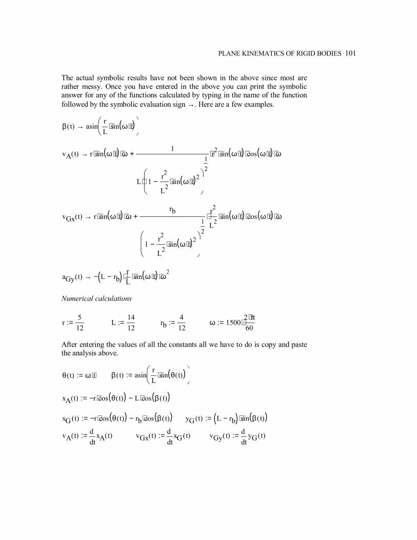
PLANE KINEMATICS OF RIGID BODIES 101
The actual symbolic results have not been shown in the above since most are rather messy. Once you have entered in the above you can print the symbolic answer for any of the functions calculated by typing in the name of the function followed by the symbolic evaluation sign →. Here are a few examples.
β t( ) asinrL
sin ω t⋅( )⋅
→
vA t( ) r sin ω t⋅( )⋅ ω⋅1
L 1r2
L2sin ω t⋅( )2
⋅−
12
⋅
r2⋅ sin ω t⋅( )⋅ cos ω t⋅( )⋅ ω⋅+→
vGx t( ) r sin ω t⋅( )⋅ ω⋅rb
1r2
L2sin ω t⋅( )2
⋅−
12
r2
L2⋅ sin ω t⋅( )⋅ cos ω t⋅( )⋅ ω⋅+→
aGy t( ) L rb−( )−rL
⋅ sin ω t⋅( )⋅ ω2
⋅→
Numerical calculations
r512
:= L1412
:= rb412
:= ω 15002 π⋅60
⋅:=
After entering the values of all the constants all we have to do is copy and paste the analysis above.
θ t( ) ω t⋅:= β t( ) asinrL
sin θ t( )( )⋅
:=
xA t( ) r− cos θ t( )( )⋅ L cos β t( )( )⋅−:= xG t( ) r− cos θ t( )( )⋅ rb cos β t( )( )⋅−:= yG t( ) L rb−( ) sin β t( )( )⋅:=
vA t( )txA t( )d
d:= vGx t( )
txG t( )d
d:= vGy t( )
tyG t( )d
d:=
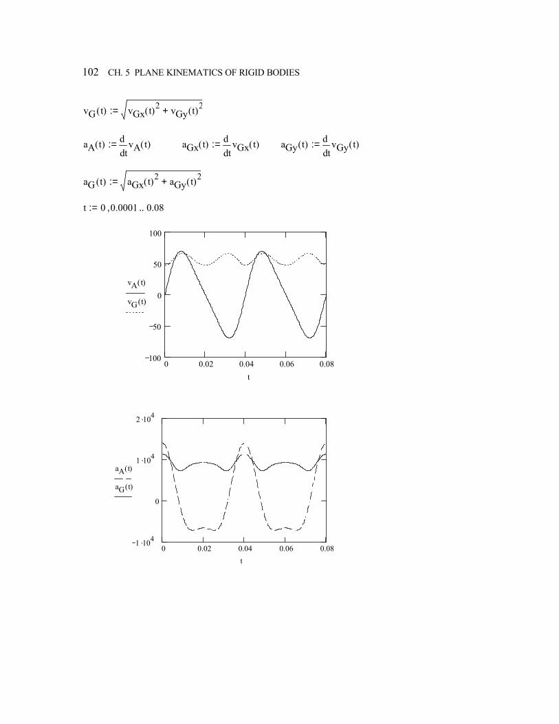
102 CH. 5 PLANE KINEMATICS OF RIGID BODIES
vG t( ) vGx t( )2 vGy t( )2+:=
aA t( )tvA t( )d
d:= aGx t( )
tvGx t( )d
d:= aGy t( )
tvGy t( )d
d:=
aG t( ) aGx t( )2 aGy t( )2+:=
t 0 0.0001, 0.08..:=
0 0.02 0.04 0.06 0.081 .104
0
1 .104
2 .104
aA t( )
aG t( )
t
0 0.02 0.04 0.06 0.08100
50
0
50
100
vA t( )
vG t( )
t
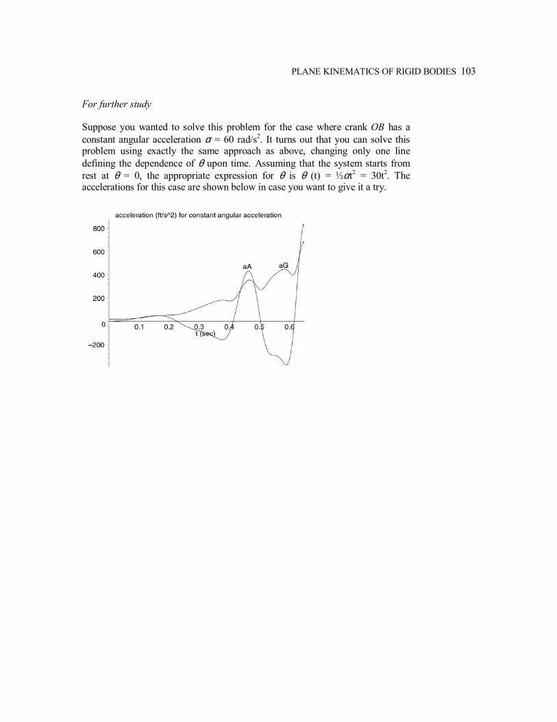
PLANE KINEMATICS OF RIGID BODIES 103
For further study Suppose you wanted to solve this problem for the case where crank OB has a constant angular acceleration α = 60 rad/s2. It turns out that you can solve this problem using exactly the same approach as above, changing only one line defining the dependence of θ upon time. Assuming that the system starts from rest at θ = 0, the appropriate expression for θ is θ (t) = ½αt2 = 30t2. The accelerations for this case are shown below in case you want to give it a try.

PLANE KINETICS OF RIGID BODIES This chapter concerns the motion (translation and rotation) of rigid bodies that results from the action of unbalanced external forces and moments. In problem 6.1, five equations are solved for five unknowns. The problem illustrates an alternative to the blunt (but straightforward) simultaneous solution of multiple equations. Instead, the equations are solved in such a way that there is never more than one unknown. In this way, the results are immediately obtained via automatic substitution in MathCad, thus avoiding some tedious algebra. The force at the hinge of a pendulum is plotted versus the angular position of the pendulum in problem 6.2. The algebra is rather simple in this case and Mathcad is used primarily for purposes of plotting. Problems 6.3 and 6.4 consider rigid bodies in general plane motion. GivenFind is used in problem 6.3 to solve two equations simultaneously for two unknowns. The maximum acceleration of a point on the rigid body is then obtained in the usual manner. The orientation at which the maximum occurs is found by setting the derivative equal to zero with this result being substituted back to find the maximum. This problem is also interesting since a very natural guess of the value for the maximum acceleration turns out to be incorrect. Problem 6.4 is an example of a kinetics problem that also requires some kinematics. The angular acceleration of a bar is determined by summing moments. The kinematic equation θαωω dd = is then integrated to obtain the angular velocity. Problem 6.5 is an interesting work and energy problem that is complicated considerably by the fact that a spring is engaged for only part of the motion of a rotating bar. Symbolic algebra simplifies this problem considerably, though it is still rather tedious. It is common in Dynamics to find problems that require a combination of methods for their solution. Problem 6.6 is a good example involving both conservation of momentum and work/energy.
6
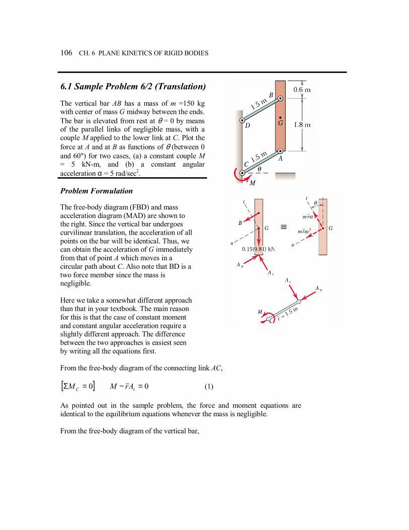
106 CH. 6 PLANE KINETICS OF RIGID BODIES
6.1 Sample Problem 6/2 (Translation) The vertical bar AB has a mass of m =150 kg with center of mass G midway between the ends. The bar is elevated from rest at θ = 0 by means of the parallel links of negligible mass, with a couple M applied to the lower link at C. Plot the force at A and at B as functions of θ (between 0 and 60°) for two cases, (a) a constant couple M = 5 kN-m, and (b) a constant angular acceleration α = 5 rad/sec2. Problem Formulation The free-body diagram (FBD) and mass acceleration diagram (MAD) are shown to the right. Since the vertical bar undergoes curvilinear translation, the acceleration of all points on the bar will be identical. Thus, we can obtain the acceleration of G immediately from that of point A which moves in a circular path about C. Also note that BD is a two force member since the mass is negligible. Here we take a somewhat different approach than that in your textbook. The main reason for this is that the case of constant moment and constant angular acceleration require a slightly different approach. The difference between the two approaches is easiest seen by writing all the equations first. From the free-body diagram of the connecting link AC, [ ]0=Σ CM 0=− tArM (1) As pointed out in the sample problem, the force and moment equations are identical to the equilibrium equations whenever the mass is negligible. From the free-body diagram of the vertical bar,
PLANE KINETICS OF RIGID BODIES 107
[ ]damM A =Σ AGAGAB rrmrrmBr θαθωθ sincoscos 2 += (2) [ ]tt amF =Σ αθ rmmgAt =− cos (3) [ ]nn amF =Σ 2sin ωθ rmmgAB n =+− (4) And, finally, the kinematics equation
∫ ∫=ω θ
θαωω0 0
dd (5)
At this point we have a total of 5 equations and 6 unknowns (M, α, ω, At, An, and B). In part (a), M is specified while in part (b) α is given. In both cases we will have 5 equations and 5 unknowns; however, it will be necessary to solve no more than one equation at a time provided they are done in the right order. This is what yields a different procedure for parts (a) and (b). Part (a) With M known we can find At from Equation (1) and then substitute the result into Equation (3) to get α as a function of θ.
rMAt =
θα cosrg
rmAt −=
As usual, notice that there is no need to make an explicit substitution of At into α. The computer will make such substitutions automatically. Now we substitute α into Equation (5) and integrate,
θθωθ
drg
rmAt∫
−=
0
2 cos21
−= θθω sin22
rg
rmAt
108 CH. 6 PLANE KINETICS OF RIGID BODIES
Finally, we can substitute into Equations (2) and (4) to find B and then An.
( )θαθωθ
sincoscos
2 +=AB
AG
rrrm
B
2sin ωθ rmmgBAn −+=
22tn AAA +=
Part (b) With α known instead of M we have to take a different approach, starting with Equations (5) and (3),
∫ ∫ ===θ θ
αθθαθαω0 0
2 222 dd
αθ rmmgAt += cos Now we can substitute into Equations (1), (2) and (4) to find M, B and then An. tArM =
( )θαθωθ
sincoscos
2 +=AB
AG
rrrm
B
2sin ωθ rmmgBAn −+=
22tn AAA +=
MathCad Worksheets Its probably easiest to create individual worksheets for parts (a) and (b).
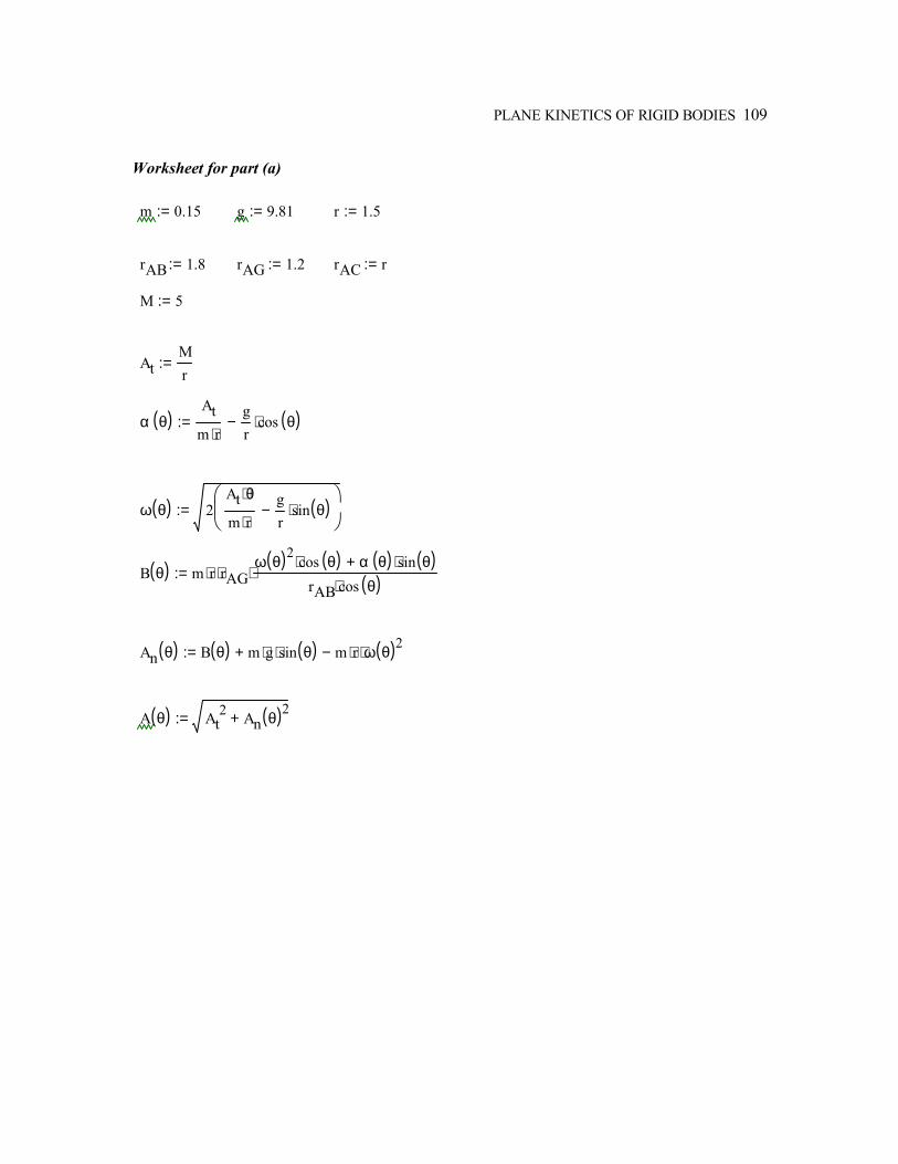
PLANE KINETICS OF RIGID BODIES 109
Worksheet for part (a)
m 0.15:= g 9.81:= r 1.5:=
rAB 1.8:= rAG 1.2:= rAC r:=
M 5:=
AtMr
:=
α θ( )At
m r⋅gr
cos θ( )⋅−:=
ω θ( ) 2At θ⋅
m r⋅gr
sin θ( )⋅−
:=
B θ( ) m r⋅ rAG⋅ω θ( )2 cos θ( )⋅ α θ( ) sin θ( )⋅+
rAB cos θ( )⋅⋅:=
An θ( ) B θ( ) m g⋅ sin θ( )⋅+ m r⋅ ω θ( )2⋅−:=
A θ( ) At2 An θ( )2+:=
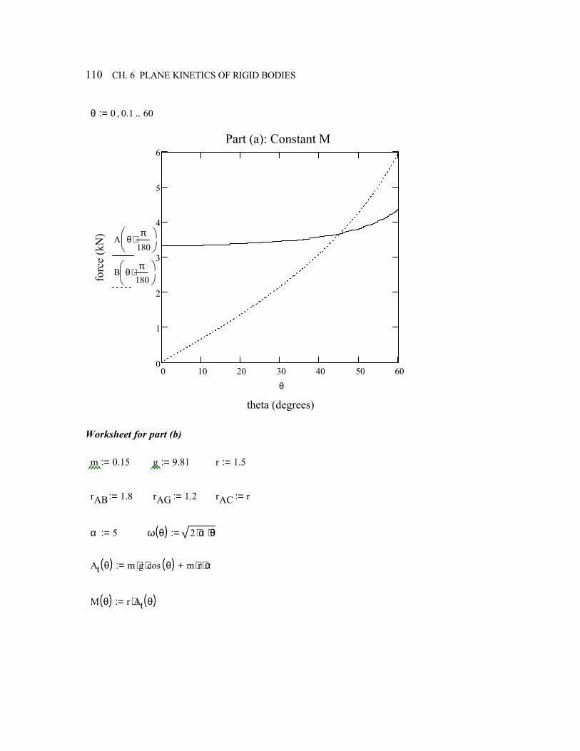
110 CH. 6 PLANE KINETICS OF RIGID BODIES
θ 0 0.1, 60..:=
0 10 20 30 40 50 600
1
2
3
4
5
6Part (a): Constant M
theta (degrees)
forc
e (k
N) A θ
π180
⋅
B θπ
180⋅
θ
Worksheet for part (b)
m 0.15:= g 9.81:= r 1.5:=
rAB 1.8:= rAG 1.2:= rAC r:=
α 5:= ω θ( ) 2 α⋅ θ⋅:=
At θ( ) m g⋅ cos θ( )⋅ m r⋅ α⋅+:=
M θ( ) r At θ( )⋅:=
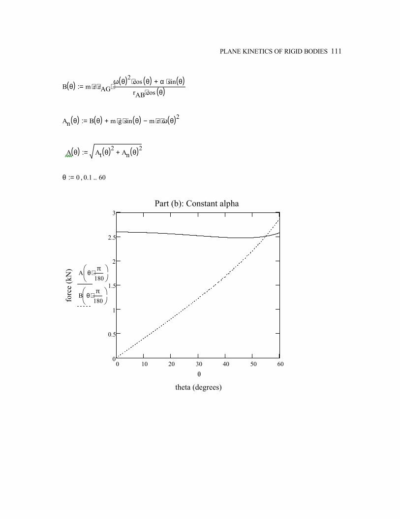
PLANE KINETICS OF RIGID BODIES 111
B θ( ) m r⋅ rAG⋅ω θ( )2 cos θ( )⋅ α sin θ( )⋅+
rAB cos θ( )⋅⋅:=
An θ( ) B θ( ) m g⋅ sin θ( )⋅+ m r⋅ ω θ( )2⋅−:=
A θ( ) At θ( )2 An θ( )2+:=
θ 0 0.1, 60..:=
0 10 20 30 40 50 600
0.5
1
1.5
2
2.5
3Part (b): Constant alpha
theta (degrees)
forc
e (k
N) A θ
π180
⋅
B θπ
180⋅
θ
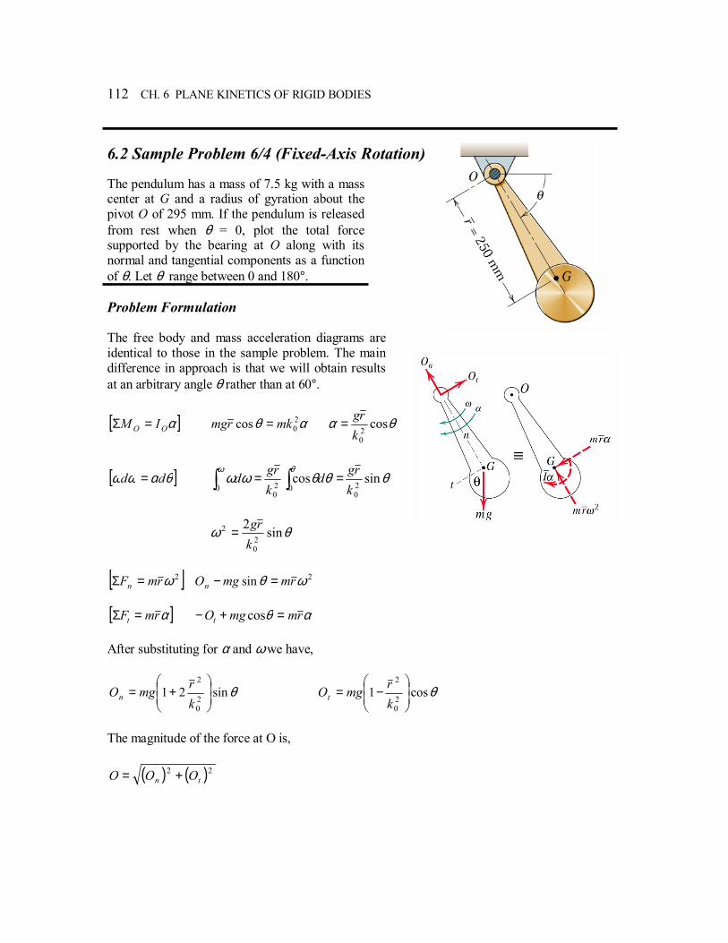
112 CH. 6 PLANE KINETICS OF RIGID BODIES
6.2 Sample Problem 6/4 (Fixed-Axis Rotation) The pendulum has a mass of 7.5 kg with a mass center at G and a radius of gyration about the pivot O of 295 mm. If the pendulum is released from rest when θ = 0, plot the total force supported by the bearing at O along with its normal and tangential components as a function of θ. Let θ range between 0 and 180°. Problem Formulation The free body and mass acceleration diagrams are identical to those in the sample problem. The main difference in approach is that we will obtain results at an arbitrary angle θ rather than at 60°.
[ ]αOO IM =Σ αθ 20cos mkrmg = θα cos
20krg=
[ ]θαωω dd = θθθωωω θ
sincos20
0 020 k
rgdk
rgd∫ ∫ ==
θω sin220
2
krg=
[ ]2ωrmFn =Σ 2sin ωθ rmmgOn =− [ ]αrmFt =Σ αθ rmmgOt =+− cos After substituting for α and ω we have,
θsin2120
2
+=
krmgOn θcos1
20
2
−=
krmgOt
The magnitude of the force at O is,
( ) ( )22tn OOO +=
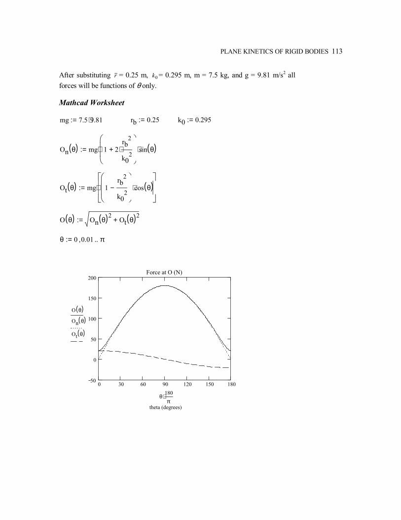
PLANE KINETICS OF RIGID BODIES 113
After substituting r = 0.25 m, 0k = 0.295 m, m = 7.5 kg, and g = 9.81 m/s2 all forces will be functions of θ only. Mathcad Worksheet mg 7.5 9.81⋅:= rb 0.25:= k0 0.295:=
On θ( ) mg 1 2rb
2
k02
⋅+
⋅ sin θ( )⋅:=
Ot θ( ) mg 1rb
2
k02
−
cos θ( )⋅
⋅:=
O θ( ) On θ( )2Ot θ( )2
+:=
θ 0 0.01, π..:=
0 30 60 90 120 150 18050
0
50
100
150
200Force at O (N)
theta (degrees)
O θ( )On θ( )
Ot θ( )
θ180π
⋅
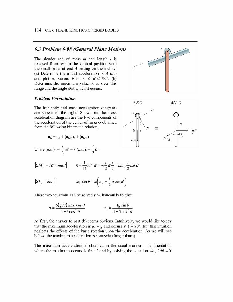
114 CH. 6 PLANE KINETICS OF RIGID BODIES
6.3 Problem 6/98 (General Plane Motion) The slender rod of mass m and length l is released from rest in the vertical position with the small roller at end A resting on the incline. (a) Determine the initial acceleration of A (aA) and plot aA versus θ for 0 ≤ θ ≤ 90°. (b) Determine the maximum value of aA over this range and the angle θ at which it occurs. Problem Formulation The free-body and mass acceleration diagrams are shown to the right. Shown on the mass acceleration diagram are the two components of the acceleration of the center of mass G obtained from the following kinematic relation,
aG = aA + (aG/A)n + (aG/A)t
where (aG/A)n = 2
2ωl =0, (aG/A)t = α
2l .
[ ]damIM A +=Σ α θαα cos22212
10 2 lmallmml A−+=
[ ]xx amF =Σ
−= θαθ cos
2sin lammg A
These two equations can be solved simultaneously to give,
( )θ
θθα 2cos34cossin/6
−= lg
θθ2cos34
sin4−
= gaA
At first, the answer to part (b) seems obvious. Intuitively, we would like to say that the maximum acceleration is aA = g and occurs at θ = 90°. But this intuition neglects the effects of the bars rotation upon the acceleration. As we will see below, the maximum acceleration is somewhat larger than g. The maximum acceleration is obtained in the usual manner. The orientation where the maximum occurs is first found by solving the equation 0/ =θddaA
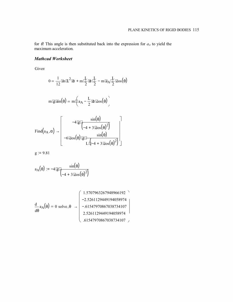
PLANE KINETICS OF RIGID BODIES 115
for θ. This angle is then substituted back into the expression for aA to yield the maximum acceleration. Mathcad Worksheet Given
0112
m⋅ L2⋅ α⋅ mL2
⋅ α⋅L2
⋅+ m aA⋅L2
⋅ cos θ( )⋅−
m g⋅ sin θ( )⋅ m aAL2
α⋅ cos θ( )⋅−
⋅
Find aA α,( )4− g⋅
sin θ( )4− 3 cos θ( )2
⋅+( )⋅
6− cos θ( )⋅ g⋅sin θ( )
L 4− 3 cos θ( )2⋅+( )⋅
⋅
→
g 9.81:=
aA θ( ) 4− g⋅sin θ( )
4− 3 cos θ( )2⋅+( )⋅:=
θaA θ( )d
d0 solve θ,
1.5707963267948966192
2.5261129449194058974−
.61547970867038734107−
2.5261129449194058974
.61547970867038734107
→
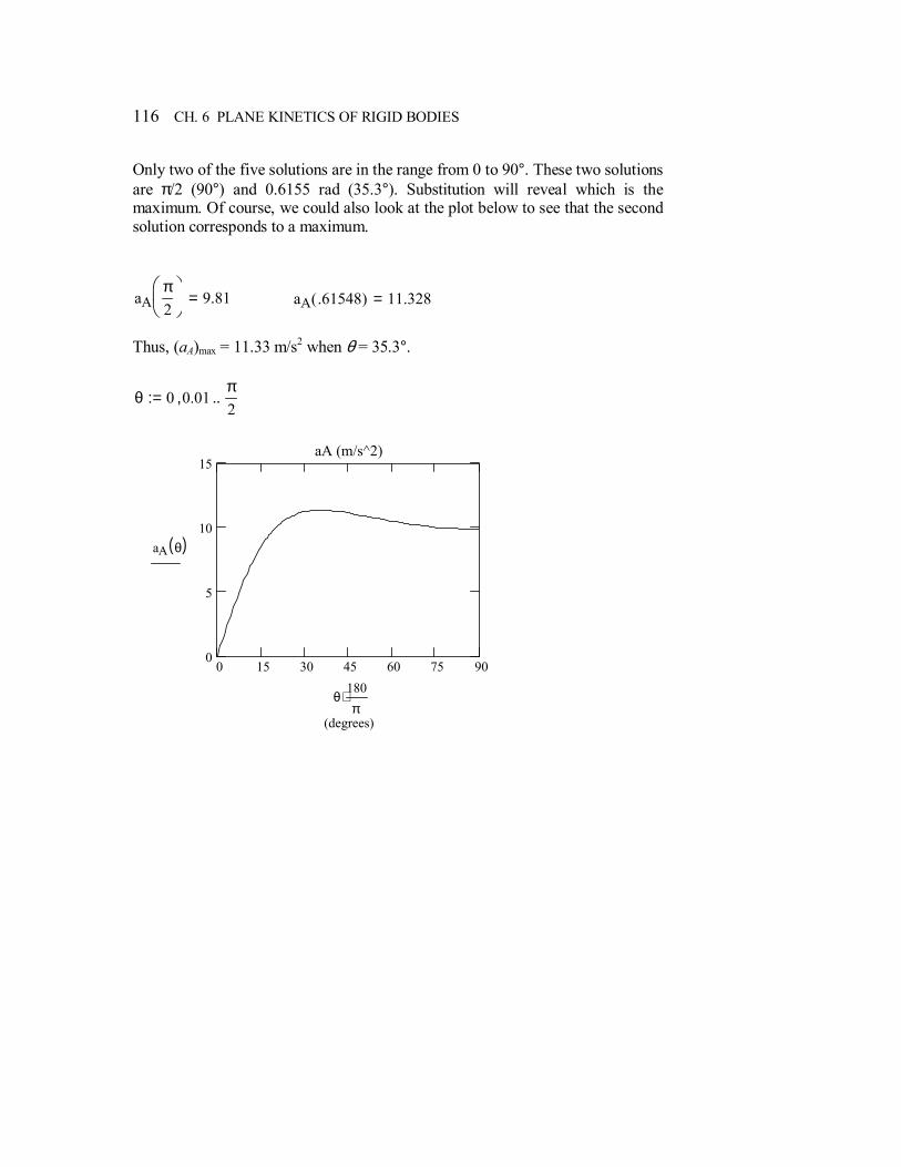
116 CH. 6 PLANE KINETICS OF RIGID BODIES
Only two of the five solutions are in the range from 0 to 90°. These two solutions are π/2 (90°) and 0.6155 rad (35.3°). Substitution will reveal which is the maximum. Of course, we could also look at the plot below to see that the second solution corresponds to a maximum.
aAπ2
9.81= aA .61548( ) 11.328= Thus, (aA)max = 11.33 m/s2 when θ = 35.3°.
θ 0 0.01,π2
..:=
0 15 30 45 60 75 900
5
10
15aA (m/s^2)
(degrees)
aA θ( )
θ180π
⋅
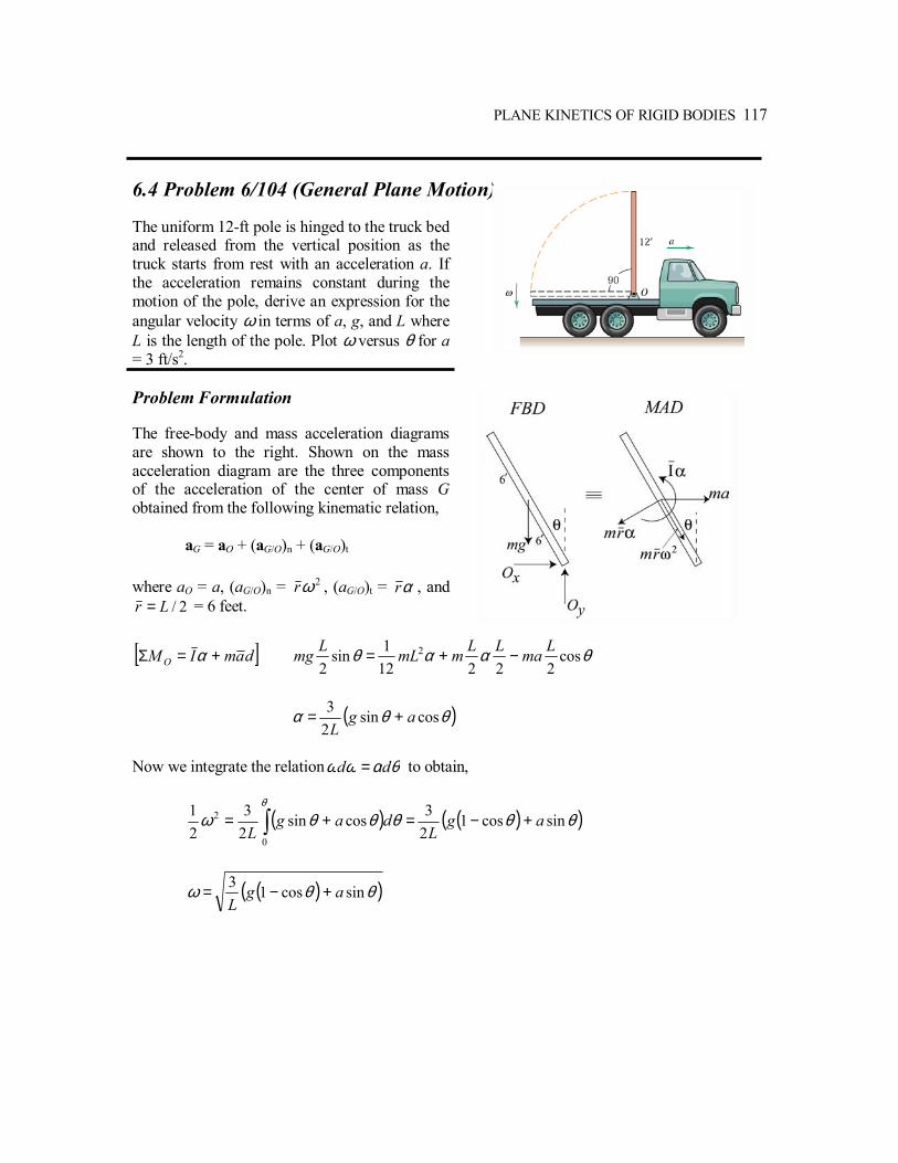
PLANE KINETICS OF RIGID BODIES 117
6.4 Problem 6/104 (General Plane Motion) The uniform 12-ft pole is hinged to the truck bed and released from the vertical position as the truck starts from rest with an acceleration a. If the acceleration remains constant during the motion of the pole, derive an expression for the angular velocity ω in terms of a, g, and L where L is the length of the pole. Plot ω versus θ for a = 3 ft/s2. Problem Formulation The free-body and mass acceleration diagrams are shown to the right. Shown on the mass acceleration diagram are the three components of the acceleration of the center of mass G obtained from the following kinematic relation,
aG = aO + (aG/O)n + (aG/O)t where aO = a, (aG/O)n = 2ωr , (aG/O)t = αr , and
2/Lr = = 6 feet.
[ ]damIM O +=Σ α θααθ cos22212
1sin2
2 LmaLLmmLLmg −+=
( )θθα cossin23 agL
+=
Now we integrate the relation θαωω dd = to obtain,
( ) ( )( )θθθθθωθ
sincos123cossin
23
21
0
2 agL
dagL
+−=+= ∫
( )( )θθω sincos13 agL
+−=
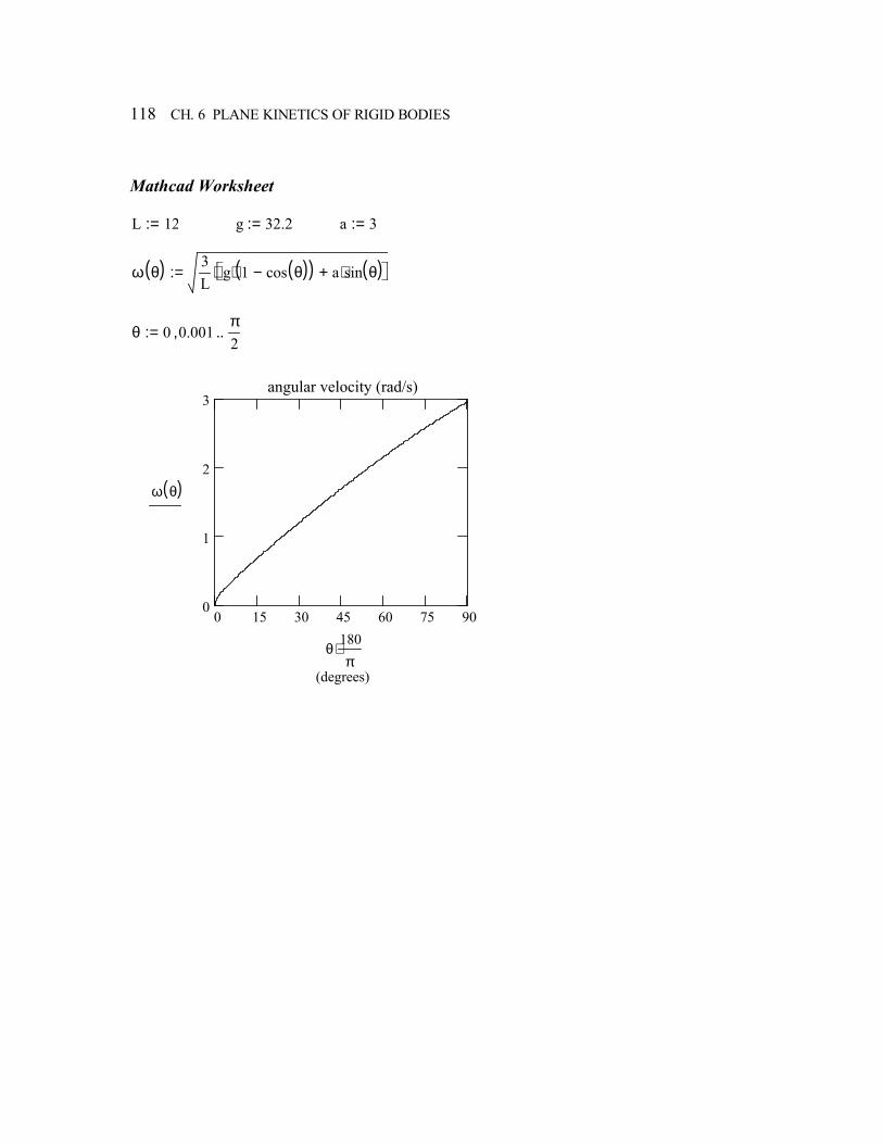
118 CH. 6 PLANE KINETICS OF RIGID BODIES
Mathcad Worksheet L 12:= g 32.2:= a 3:=
ω θ( ) 3L
g 1 cos θ( )−( )⋅ a sin θ( )⋅+ ⋅:=
θ 0 0.001,π2
..:=
0 15 30 45 60 75 900
1
2
3angular velocity (rad/s)
(degrees)
ω θ( )
θ180π
⋅
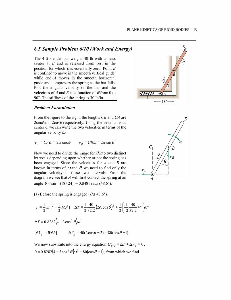
PLANE KINETICS OF RIGID BODIES 119
6.5 Sample Problem 6/10 (Work and Energy) The 4-ft slender bar weighs 40 lb with a mass center at B and is released from rest in the position for which θ is essentially zero. Point B is confined to move in the smooth vertical guide, while end A moves in the smooth horizontal guide and compresses the spring as the bar falls. Plot the angular velocity of the bar and the velocities of A and B as a function of θ from 0 to 90°. The stiffness of the spring is 30 lb/in. Problem Formulation From the figure to the right, the lengths CB and CA are 2sinθ and 2cosθ respectively. Using the instantaneous center C we can write the two velocities in terms of the angular velocity ω.
θωω cos2== CAvA θωω sin2== CBvB Now we need to divide the range for θ into two distinct intervals depending upon whether or not the spring has been engaged. Since the velocities for A and B are known in terms of ω and θ, we need to find only the angular velocity in these two intervals. From the diagram we see that A will first contact the spring at an angle )24/18(sin 1−=θ = 0.8481 rads (48.6°). (a) Before the spring is engaged (θ ≤ 48.6°).
]21
21[ 22 ωIvmT += ( ) 222 4
2.3240
121
21cos2
2.3240
21 ωθω
+=∆T
( ) 22cos348282.0 ωθ−=∆T
][ hWVg ∆=∆ )1(cos80)2cos2(40 −=−=∆ θθgV
We now substitute into the energy equation 021 =∆+∆=′− gVTU ,
( ) ( )1cos80cos348282.00 22 −+−= θωθ , from which we find
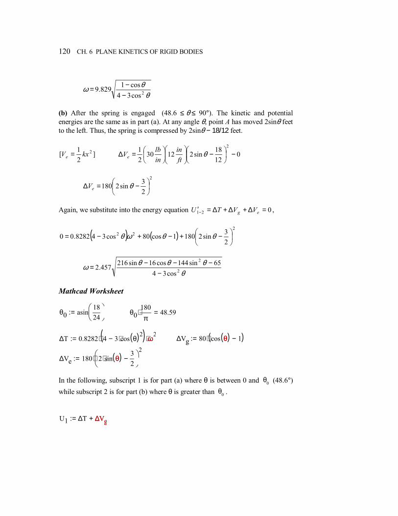
120 CH. 6 PLANE KINETICS OF RIGID BODIES
θθω 2cos34
cos1829.9−−=
(b) After the spring is engaged (48.6 ≤ θ ≤ 90°). The kinetic and potential energies are the same as in part (a). At any angle θ, point A has moved 2sinθ feet to the left. Thus, the spring is compressed by 2sinθ − 18/12 feet.
]21[ 2kxVe = 0
1218
sin2123021 2
−
−
=∆ θ
ftin
inlbVe
2
23sin2180
−=∆ θeV
Again, we substitute into the energy equation 021 =∆+∆+∆=′− eg VVTU ,
( ) ( )2
22
23sin21801cos80cos348282.00
−+−+−= θθωθ
θθθθω 2
2
cos3465sin144cos16sin216457.2
−−−−=
Mathcad Worksheet
θ0 asin1824
:= θ0180π
⋅ 48.59=
∆T 0.8282 4 3 cos θ( )2⋅−( )⋅ ω
2⋅:= ω ∆Vg 80 cos θ( ) 1−( )⋅:= θ
∆Ve 180 2 sin θ( )⋅32
−
2⋅:= θ
In the following, subscript 1 is for part (a) where θ is between 0 and θ0 (48.6°) while subscript 2 is for part (b) where θ is greater than θ0 .
U1 ∆T ∆Vg+:= ∆Vg
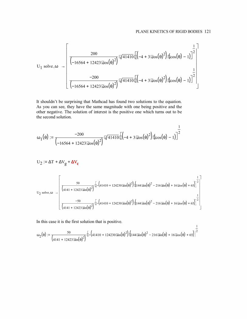
PLANE KINETICS OF RIGID BODIES 121
U1 solve ω,
200
16564− 12423 cos θ( )2⋅+( ) 41410⋅ 4− 3 cos θ( )2
⋅+( ) cos θ( ) 1−( )⋅
12
⋅
200−
16564− 12423 cos θ( )2⋅+( ) 41410⋅ 4− 3 cos θ( )2
⋅+( ) cos θ( ) 1−( )⋅
12
⋅
→
It shouldnt be surprising that Mathcad has found two solutions to the equation. As you can see, they have the same magnitude with one being positive and the other negative. The solution of interest is the positive one which turns out to be the second solution.
ω1 θ( ) 200−
16564− 12423 cos θ( )2⋅+( ) 41410⋅ 4− 3 cos θ( )2
⋅+( ) cos θ( ) 1−( )⋅
12
⋅:=
U2 ∆T ∆Vg+ ∆Ve+:= ∆Ve
U2 solve ω,
50
4141 12423 sin θ( )2⋅+( ) 41410 124230 sin θ( )2
⋅+( )− 144 sin θ( )2⋅ 216 sin θ( )⋅− 16 cos θ( )⋅+ 65+( )⋅
12
⋅
50−
4141 12423 sin θ( )2⋅+( ) 41410 124230 sin θ( )2
⋅+( )− 144 sin θ( )2⋅ 216 sin θ( )⋅− 16 cos θ( )⋅+ 65+( )⋅
12
⋅
→
In this case it is the first solution that is positive.
ω2 θ( ) 50
4141 12423 sin θ( )2⋅+( ) 41410 124230 sin θ( )2
⋅+( )− 144 sin θ( )2⋅ 216 sin θ( )⋅− 16 cos θ( )⋅+ 65+( )⋅
12
⋅:=
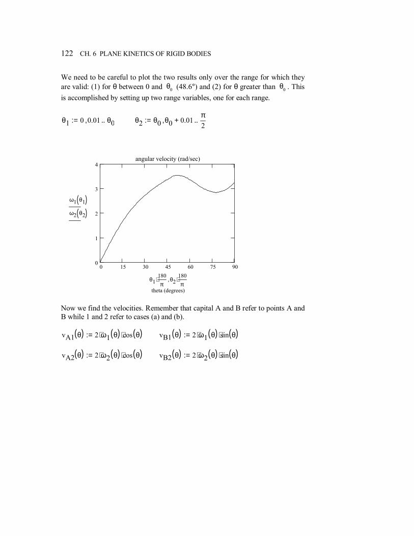
122 CH. 6 PLANE KINETICS OF RIGID BODIES
We need to be careful to plot the two results only over the range for which they are valid: (1) for θ between 0 and θ0 (48.6°) and (2) for θ greater than θ0 . This is accomplished by setting up two range variables, one for each range.
θ1 0 0.01, θ0..:= θ2 θ0 θ0 0.01+,π2
..:=
0 15 30 45 60 75 900
1
2
3
4angular velocity (rad/sec)
theta (degrees)
ω1 θ1( )ω2 θ2( )
θ1180π
⋅ θ2180π
⋅,
Now we find the velocities. Remember that capital A and B refer to points A and B while 1 and 2 refer to cases (a) and (b). vA1 θ( ) 2 ω1 θ( )⋅ cos θ( )⋅:= vB1 θ( ) 2 ω1 θ( )⋅ sin θ( )⋅:=
vA2 θ( ) 2 ω2 θ( )⋅ cos θ( )⋅:= vB2 θ( ) 2 ω2 θ( )⋅ sin θ( )⋅:=
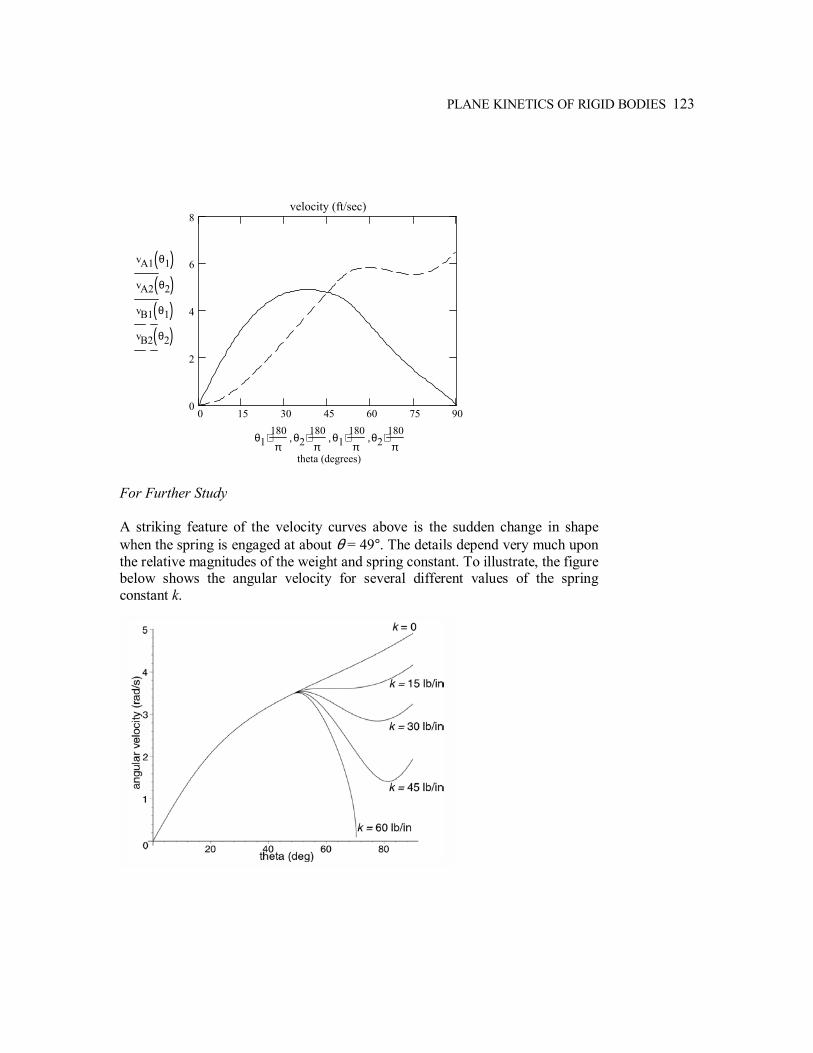
PLANE KINETICS OF RIGID BODIES 123
0 15 30 45 60 75 900
2
4
6
8velocity (ft/sec)
theta (degrees)
vA1 θ1( )vA2 θ2( )vB1 θ1( )vB2 θ2( )
θ1180π
⋅ θ2180π
⋅, θ1180π
⋅, θ2180π
⋅,
For Further Study A striking feature of the velocity curves above is the sudden change in shape when the spring is engaged at about θ = 49°. The details depend very much upon the relative magnitudes of the weight and spring constant. To illustrate, the figure below shows the angular velocity for several different values of the spring constant k.
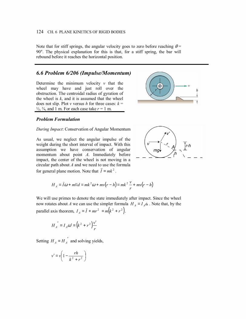
124 CH. 6 PLANE KINETICS OF RIGID BODIES
Note that for stiff springs, the angular velocity goes to zero before reaching θ = 90°. The physical explanation for this is that, for a stiff spring, the bar will rebound before it reaches the horizontal position. 6.6 Problem 6/206 (Impulse/Momentum) Determine the minimum velocity v that the wheel may have and just roll over the obstruction. The centroidal radius of gyration of the wheel is k, and it is assumed that the wheel does not slip. Plot v versus h for three cases: k = ½, ¾, and 1 m. For each case take r = 1 m. Problem Formulation During Impact: Conservation of Angular Momentum As usual, we neglect the angular impulse of the weight during the short interval of impact. With this assumption we have conservation of angular momentum about point A. Immediately before impact, the center of the wheel is not moving in a circular path about A and we need to use the formula for general plane motion. Note that 2mkI = .
( ) ( )hrmvrvmkhrmvmkdvmIH A −+=−+=+= 22ωω
We will use primes to denote the state immediately after impact. Since the wheel now rotates about A we can use the simpler formula ωAA IH = . Note that, by the parallel axis theorem, 2mrII A += ( )22 rkm += .
( )rvrkIH AA′
+=′=′ 22ω
Setting ′= AA HH and solving yields,
+−=′
221rk
rhvv
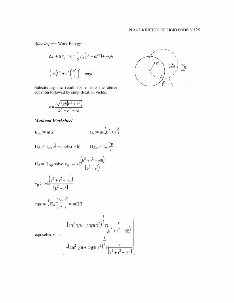
PLANE KINETICS OF RIGID BODIES 125
After Impact: Work-Energy
( ) mghIVT Ag +′−==∆+∆ 220210 ω
( ) mghrvrkm =
′
+2
22
21
Substituting the result for v′ into the above equation followed by simplification yields,
( )rhrkrkghr
v−++
= 22
222
Mathcad Worksheet
Ibar m k2⋅:= k IA m k2 r2+( )⋅:= r
HA Ibarvr
⋅ m v⋅ r h−( )⋅+:= h HAp IAvpr
⋅:=r
HA HAp solve vp, vk2 r2 r h⋅−+( )
k2 r2+( )⋅→
vp vk2 r2 r h⋅−+( )
k2 r2+( )⋅:=h
eqn12
IA⋅vpr
2
⋅ m g⋅ h⋅:= h
eqn solve v,
2 r2⋅ g⋅ h⋅ 2 g⋅ h⋅ k2⋅+( )12 r
k2 r2 r h⋅−+( )⋅
2 r2⋅ g⋅ h⋅ 2 g⋅ h⋅ k2⋅+( )12
−r
k2 r2 r h⋅−+( )⋅
→
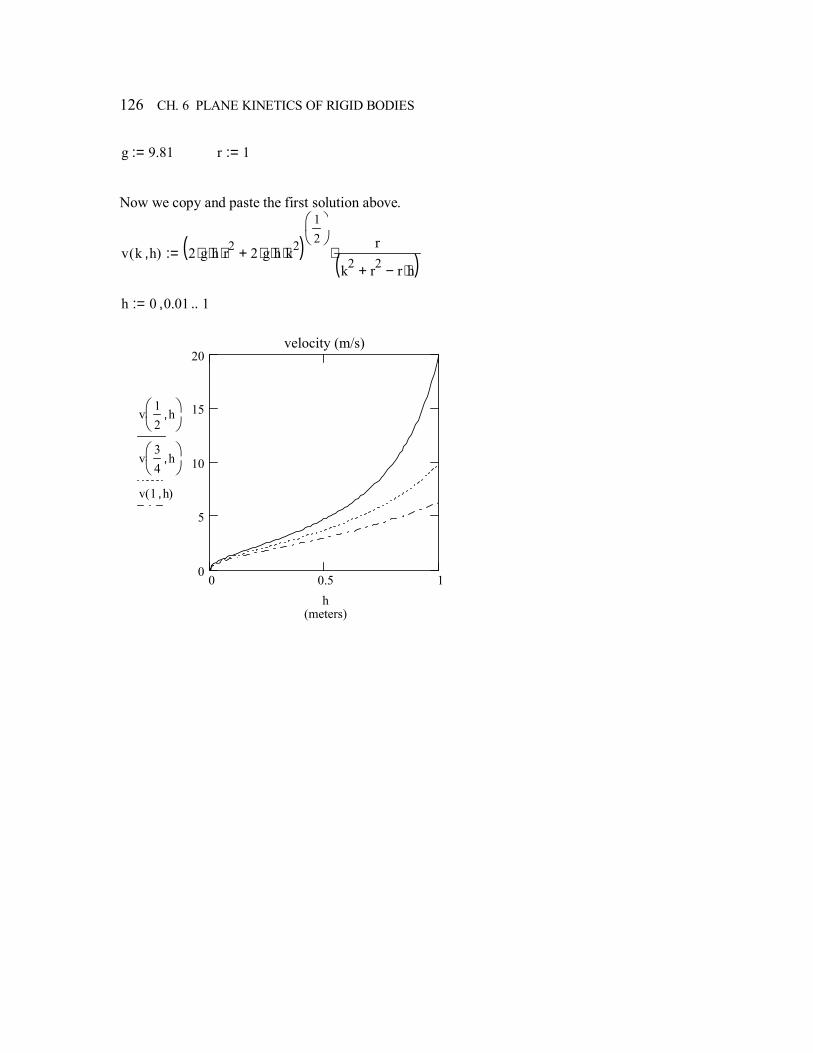
126 CH. 6 PLANE KINETICS OF RIGID BODIES
g 9.81:= r 1:=
Now we copy and paste the first solution above.
v k h,( ) 2 g⋅ h⋅ r2⋅ 2 g⋅ h⋅ k2⋅+( )12 r
k2 r2 r h⋅−+( )⋅:=
h 0 0.01, 1..:=
0 0.5 10
5
10
15
20velocity (m/s)
(meters)
v12
h,
v34
h,
v 1 h,( )
h
INTRODUCTION TO THREE- DIMENSIONAL DYNAMICS OF RIGID BODIES This chapter presents a brief introduction to rigid body dynamics in three dimensions. In problem 7.1, the general 3-D motion of three connected bars is investigated. In particular, the angular velocities of two of the bars are plotted versus the length of the third bar. GivenFind is used to solve four equations symbolically for four unknowns. In problem 7.2 we consider a bent plate rotating about a fixed axis. The problem illustrates a simplified version of what engineers might do in a real design situation. Two dimensions of the bent plate are left as variables and the objective of the problem is to find all suitable values of those dimensions which satisfy several constraints simultaneously. Here we illustrate a graphical approach to this type of design problem.
7
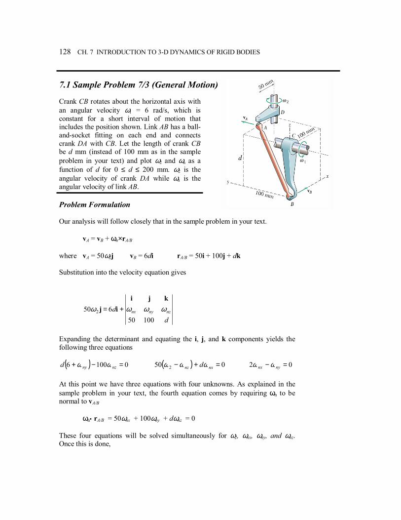
128 CH. 7 INTRODUCTION TO 3-D DYNAMICS OF RIGID BODIES
7.1 Sample Problem 7/3 (General Motion) Crank CB rotates about the horizontal axis with an angular velocity ω1 = 6 rad/s, which is constant for a short interval of motion that includes the position shown. Link AB has a ball-and-socket fitting on each end and connects crank DA with CB. Let the length of crank CB be d mm (instead of 100 mm as in the sample problem in your text) and plot ω2 and ωn as a function of d for 0 ≤ d ≤ 200 mm. ω2 is the angular velocity of crank DA while ωn is the angular velocity of link AB. Problem Formulation Our analysis will follow closely that in the sample problem in your text.
vA = vB + ωn×rA/B where vA = 50ω2j vB = 6di rA/B = 50i + 100j + dk Substitution into the velocity equation gives
dd nznynx
10050650 2 ωωωω
kjiij +=
Expanding the determinant and equating the i, j, and k components yields the following three equations
( ) 01006 =−+ nznyd ωω ( ) 050 2 =+− nxnz dωωω 02 =− nynx ωω At this point we have three equations with four unknowns. As explained in the sample problem in your text, the fourth equation comes by requiring ωn to be normal to vA/B
ωn• rA/B = 50ωnx + 100ωny + dωnz = 0 These four equations will be solved simultaneously for ω2, ωnx, ωny, and ωnz. Once this is done,
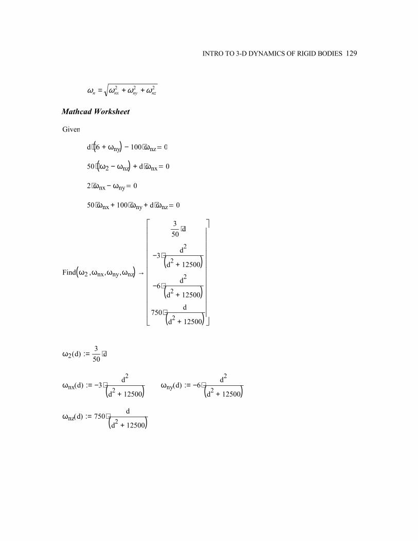
INTRO TO 3-D DYNAMICS OF RIGID BODIES 129
222nznynxn ωωωω ++=
Mathcad Worksheet Given
d 6 ωny+( )⋅ 100 ωnz⋅− 0
50 ω2 ωnz−( )⋅ d ωnx⋅+ 0
2 ωnx⋅ ωny− 0
50 ωnx⋅ 100 ωny⋅+ d ωnz⋅+ 0
Find ω2 ωnx, ωny, ωnz,( )
350
d⋅
3−d2
d2 12500+( )⋅
6−d2
d2 12500+( )⋅
750d
d2 12500+( )⋅
→
ω2 d( )350
d⋅:=
ωnx d( ) 3−d2
d2 12500+( )⋅:=
ωny d( ) 6−d2
d2 12500+( )⋅:=
ωnz d( ) 750d
d2 12500+( )⋅:=
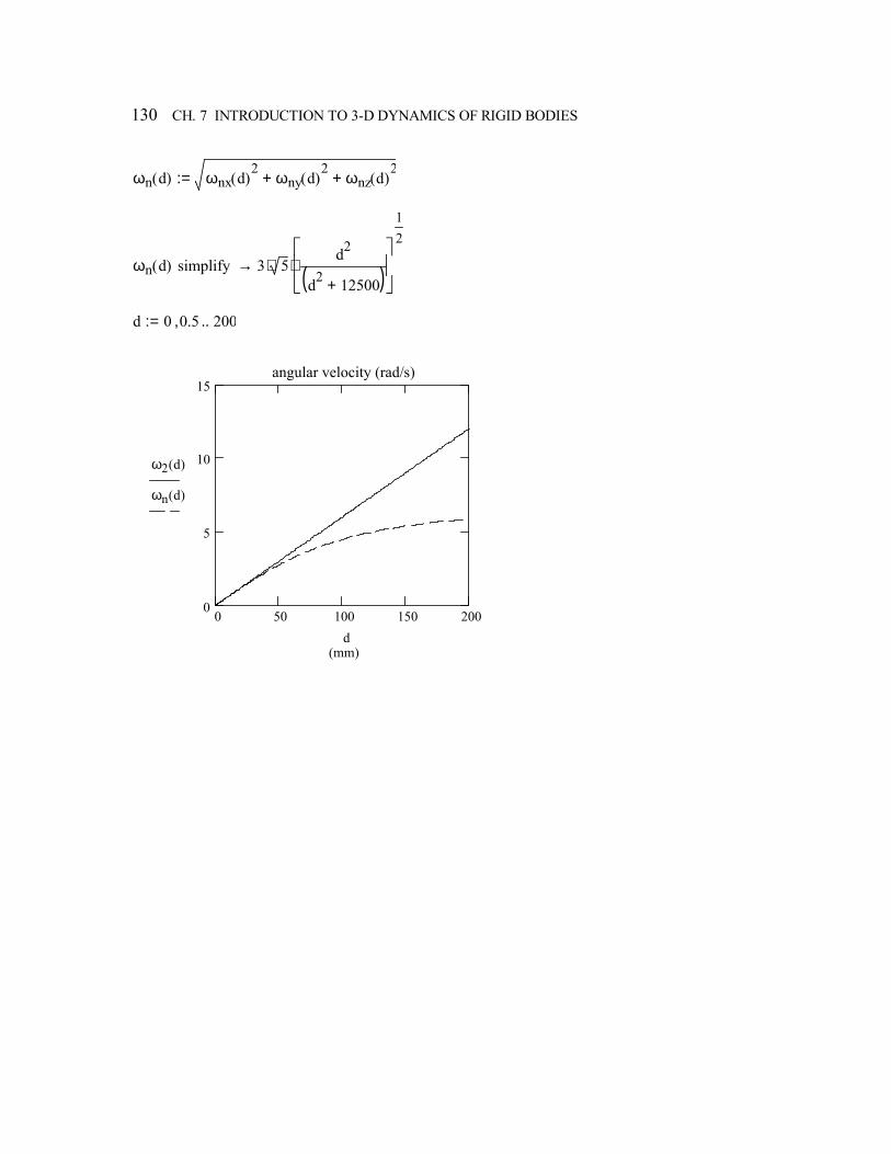
130 CH. 7 INTRODUCTION TO 3-D DYNAMICS OF RIGID BODIES
ωn d( ) ωnx d( )2
ωny d( )2
+ ωnz d( )2
+:=
ωn d( ) simplify 3 5⋅d2
d2 12500+( )
12
⋅→
d 0 0.5, 200..:=
0 50 100 150 2000
5
10
15angular velocity (rad/s)
(mm)
ω2 d( )
ωn d( )
d
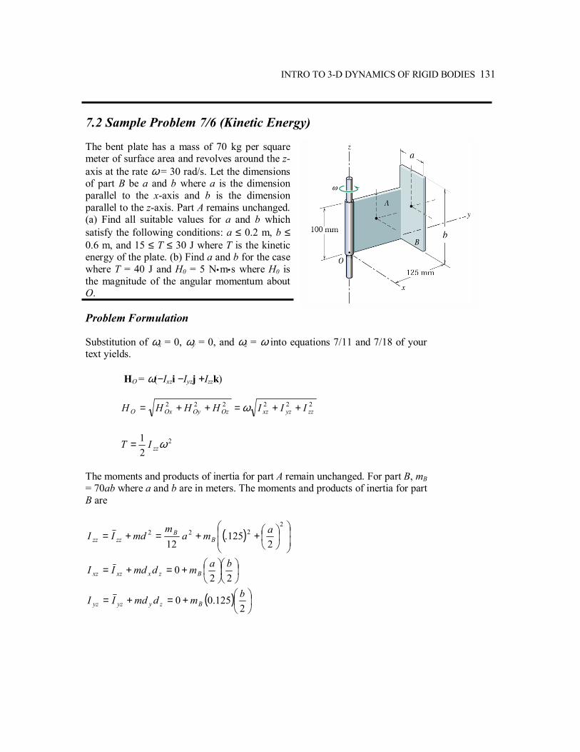
INTRO TO 3-D DYNAMICS OF RIGID BODIES 131
7.2 Sample Problem 7/6 (Kinetic Energy) The bent plate has a mass of 70 kg per square meter of surface area and revolves around the z-axis at the rate ω = 30 rad/s. Let the dimensions of part B be a and b where a is the dimension parallel to the x-axis and b is the dimension parallel to the z-axis. Part A remains unchanged. (a) Find all suitable values for a and b which satisfy the following conditions: a ≤ 0.2 m, b ≤ 0.6 m, and 15 ≤ T ≤ 30 J where T is the kinetic energy of the plate. (b) Find a and b for the case where T = 40 J and H0 = 5 N•m•s where H0 is the magnitude of the angular momentum about O. Problem Formulation Substitution of ωx = 0, ωy = 0, and ωz = ω into equations 7/11 and 7/18 of your text yields. HO = ω(−Ixzi −Iyzj +Izzk) 222222
zzyzxzOzOyOxO IIIHHHH ++=++= ω
2
21 ωzzIT =
The moments and products of inertia for part A remain unchanged. For part B, mB = 70ab where a and b are in meters. The moments and products of inertia for part B are
( )
++=+=
2222
2125.
12ama
mmdII B
Bzzzz
+=+=
220 bamdmdII Bzxxzxz
( )
+=+=
2125.00 bmdmdII Bzyyzyz
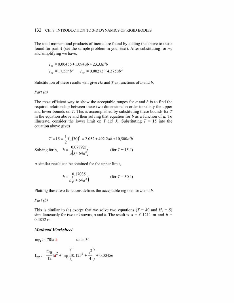
132 CH. 7 INTRODUCTION TO 3-D DYNAMICS OF RIGID BODIES
The total moment and products of inertia are found by adding the above to those found for part A (see the sample problem in your text). After substituting for mB and simplifying we have, baabIzz
333.23094.100456.0 ++= 225.17 baI xz = 2375.400273.0 abI yz += Substitution of these results will give HO and T as functions of a and b. Part (a) The most efficient way to show the acceptable ranges for a and b is to find the required relationship between these two dimensions in order to satisfy the upper and lower bounds on T. This is accomplished by substituting these bounds for T in the equation above and then solving that equation for b as a function of a. To illustrate, consider the lower limit on T (15 J). Substituting T = 15 into the equation above gives
( ) baabIT zz32 500,102.492052.230
2115 ++===
Solving for b, ( )2643078921.0
aab
+= (for T = 15 J)
A similar result can be obtained for the upper limit,
( )264317035.0
aab
+= (for T = 30 J)
Plotting these two functions defines the acceptable regions for a and b. Part (b) This is similar to (a) except that we solve two equations (T = 40 and H0 = 5) simultaneously for two unknowns, a and b. The result is a = 0.1211 m and b = 0.4852 m. Mathcad Worksheet mB 70 a⋅ b⋅:= b ω 30:=
IzzmB12
a2⋅ mB 0.1252 a2
4+
⋅+ 0.00456+:= a
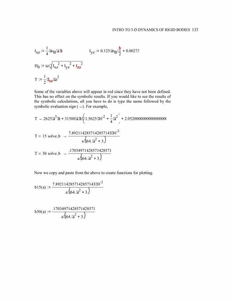
INTRO TO 3-D DYNAMICS OF RIGID BODIES 133
Ixz14
mB⋅ a⋅ b⋅:= b Iyz 0.125 mB⋅b2
⋅ 0.00273+:=b
H0 ω Ixz2 Iyz
2+ Izz2+⋅:= Izz
T12
Izz⋅ ω2
⋅:= Izz
Some of the variables above will appear in red since they have not been defined. This has no effect on the symbolic results. If you would like to see the results of the symbolic calculations, all you have to do is type the name followed by the symbolic evaluation sign (→). For example,
T 2625 a3⋅ b⋅ 31500 a⋅ b⋅ 1.5625 10-2⋅14
a2⋅+
⋅+ 2.0520000000000000000+→
T 15 solve b,7.8921142857142857143 10-2⋅
a 64. a2⋅ 3.+( )⋅→
T 30 solve b,.17034971428571428571
a 64. a2⋅ 3.+( )⋅→
Now we copy and paste from the above to create functions for plotting.
b15 a( )7.8921142857142857143 10-2⋅
a 64. a2⋅ 3.+( )⋅:=
b30 a( ).17034971428571428571
a 64. a2⋅ 3.+( )⋅:=
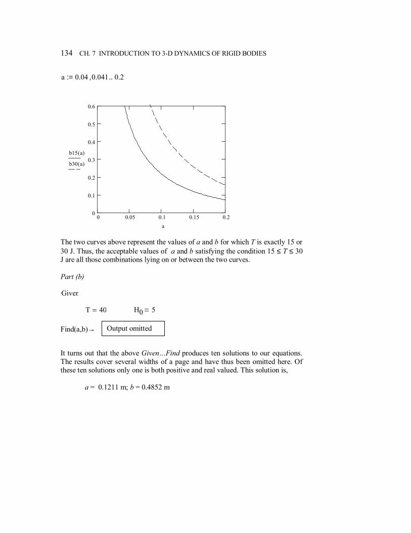
134 CH. 7 INTRODUCTION TO 3-D DYNAMICS OF RIGID BODIES
a 0.04 0.041, 0.2..:=
0 0.05 0.1 0.15 0.20
0.1
0.2
0.3
0.4
0.5
0.6
b15 a( )
b30 a( )
a
The two curves above represent the values of a and b for which T is exactly 15 or 30 J. Thus, the acceptable values of a and b satisfying the condition 15 ≤ T ≤ 30 J are all those combinations lying on or between the two curves. Part (b) Given
T 40 H0 5 Find(a,b)→ It turns out that the above GivenFind produces ten solutions to our equations. The results cover several widths of a page and have thus been omitted here. Of these ten solutions only one is both positive and real valued. This solution is, a = 0.1211 m; b = 0.4852 m
Output omitted
VIBRATION AND TIME RESPONSE This chapter considers an important class of Dynamics problems that involve linear or angular oscillations of a body or structure about some equilibrium position or configuration. Very few of the homework problems in your text require you to actually plot the oscillations of a body versus time. For this reason, all of the problems in this chapter will involve such plots. This is very useful in visualizing the time response of a vibrating system, especially for the case of damped or forced vibrations. Problem 8.1 looks at the effects of damping coefficient upon time response while Problem 8.3 considers the effects of initial conditions.
8
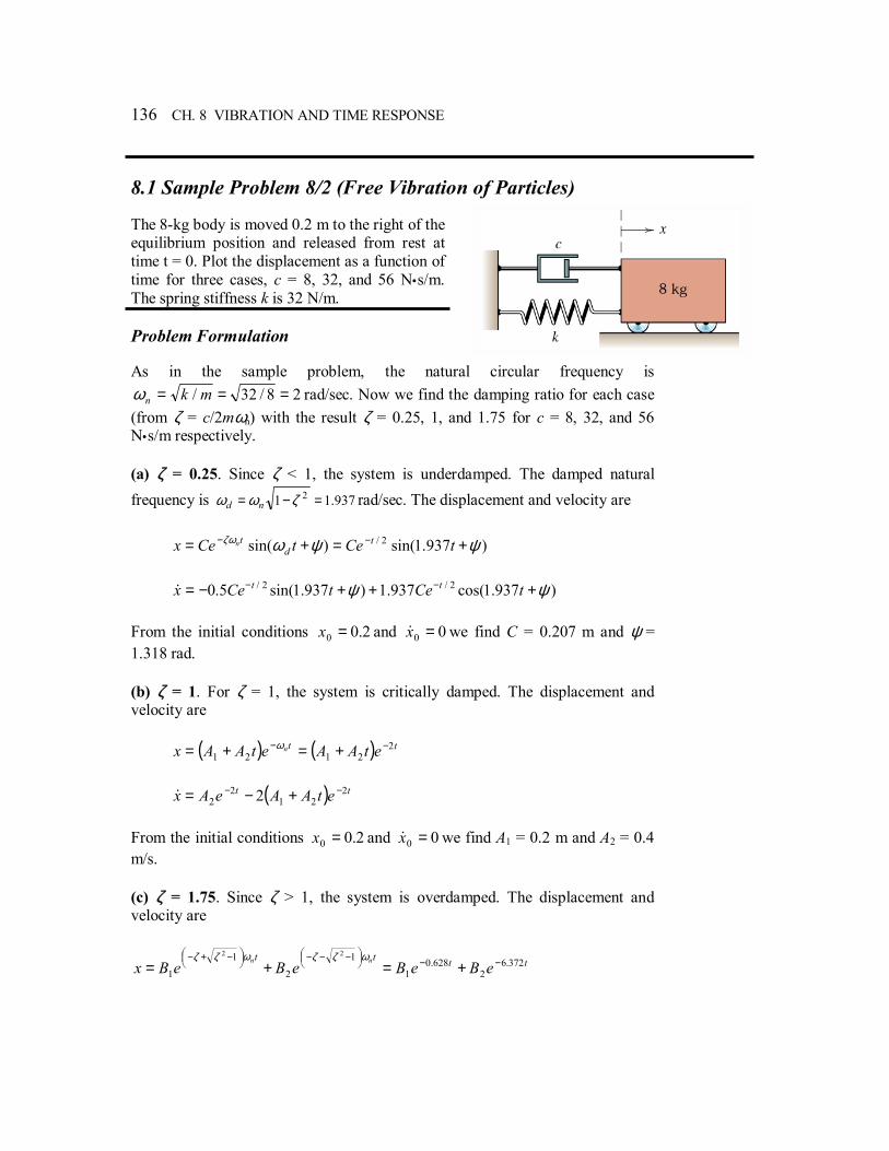
136 CH. 8 VIBRATION AND TIME RESPONSE
8.1 Sample Problem 8/2 (Free Vibration of Particles) The 8-kg body is moved 0.2 m to the right of the equilibrium position and released from rest at time t = 0. Plot the displacement as a function of time for three cases, c = 8, 32, and 56 N•s/m. The spring stiffness k is 32 N/m. Problem Formulation As in the sample problem, the natural circular frequency is
28/32/ === mknω rad/sec. Now we find the damping ratio for each case (from ζ = c/2mωn) with the result ζ = 0.25, 1, and 1.75 for c = 8, 32, and 56 N•s/m respectively. (a) ζ = 0.25. Since ζ < 1, the system is underdamped. The damped natural frequency is 937.11 2 =−= ζωω nd rad/sec. The displacement and velocity are )937.1sin()sin( 2/ ψψωζω +=+= −− tCetCex t
dtn
)937.1cos(937.1)937.1sin(5.0 2/2/ ψψ +++−= −− tCetCex tt& From the initial conditions 2.00 =x and 00 =x& we find C = 0.207 m and ψ = 1.318 rad. (b) ζ = 1. For ζ = 1, the system is critically damped. The displacement and velocity are ( ) ( ) tt etAAetAAx n 2
2121−− +=+= ω
( ) tt etAAeAx 2
212
2 2 −− +−=& From the initial conditions 2.00 =x and 00 =x& we find A1 = 0.2 m and A2 = 0.4 m/s. (c) ζ = 1.75. Since ζ > 1, the system is overdamped. The displacement and velocity are
tttteBeBeBeBx nn 372.6
2628.0
1
1
2
1
1
22−−
−−−
−+−
+=+=ωζζωζζ
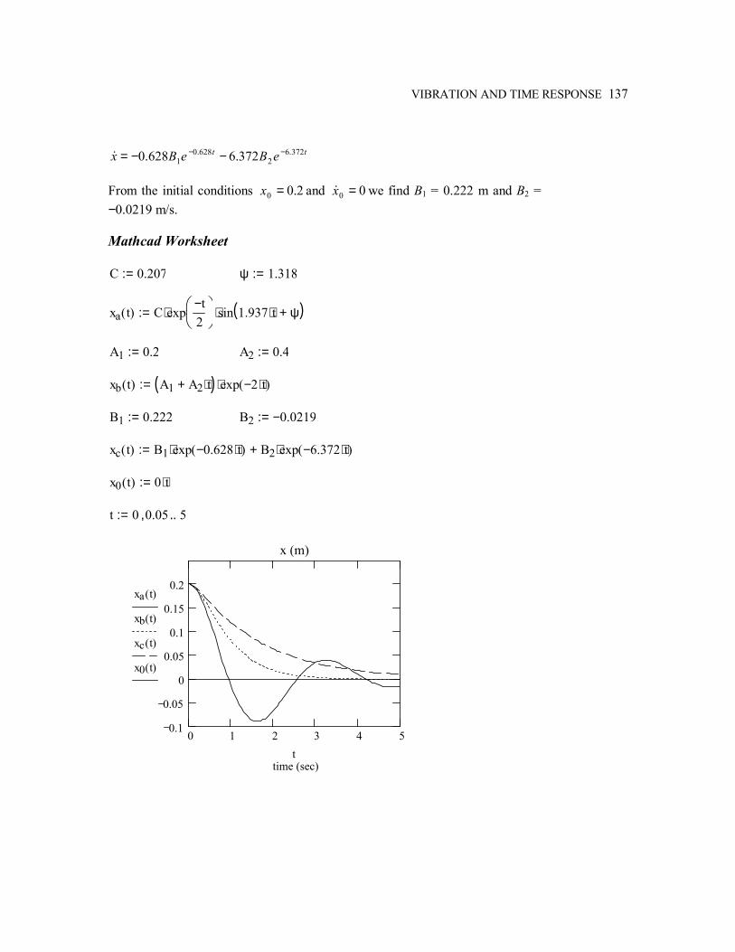
VIBRATION AND TIME RESPONSE 137
tt eBeBx 372.6
2628.0
1 372.6628.0 −− −−=& From the initial conditions 2.00 =x and 00 =x& we find B1 = 0.222 m and B2 = −0.0219 m/s. Mathcad Worksheet C 0.207:= ψ 1.318:=
xa t( ) C expt−
2
⋅ sin 1.937 t⋅ ψ+( )⋅:=
A1 0.2:= A2 0.4:= xb t( ) A1 A2 t⋅+( ) exp 2− t⋅( )⋅:= B1 0.222:= B2 0.0219−:= xc t( ) B1 exp 0.628− t⋅( )⋅ B2 exp 6.372− t⋅( )⋅+:= x0 t( ) 0 t⋅:= t 0 0.05, 5..:=
0 1 2 3 4 50.1
0.05
0
0.05
0.1
0.15
0.2
x (m)
time (sec)
xa t( )
xb t( )
xc t( )
x0 t( )
t
138 CH. 8 VIBRATION AND TIME RESPONSE
8.2 Problem 8/139 (Damped Free Vibration) The mass of a critically damped system having a natural frequency nω is released from rest at an initial displacement x0. (a) Determine the time t required for the mass to reach the position
01.0 xx = if 4=nω rad/s. (b) Plot the non-dimensional displacement x/x0 for nω = 2, 4, and 8 rad/s. Problem Formulation Start with the equation for the critically damped case on page 606 of your text. ( ) tnetAAx ω−+= 21 First we have to evaluate the constants in terms of x0 using the initial conditions. This will require the derivative of x. ( ) t
nt nn etAAeAx ωω ω −− +−= 212&
Now, substituting the initial conditions, ( ) 100 Axtx === ( ) nAAtx ω1200 −===& These two equations give 01 xA = and nxA ω02 = ( ) t
nnetxxx ωω −+= 00
or ( ) t
nnet ωωη −+= 1
where η is the non-dimensional displacement x/x0. Part (a) will require the solution to the equation
VIBRATION AND TIME RESPONSE 139
( ) tet 4411.0 −+= For part (b) we will simply plot η for three different natural frequencies nω . MathCad Worksheet
η ωn t,( ) 1 ωn t⋅+( ) eωn− t⋅
⋅:=
Part (a)
Given
η 4 t,( ) 0.1
Find t( ) .24044468956330014201− .97243004246685726448( )→ Thus, the time t required for the mass to reach the position 01.0 xx = when
4=nω rad/s is t = 0.972 sec. Part (b)
t 0 0.05, 3..:=
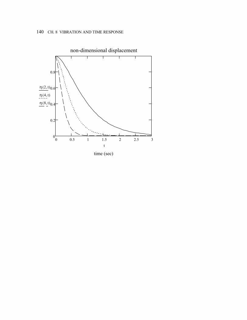
140 CH. 8 VIBRATION AND TIME RESPONSE
0 0.5 1 1.5 2 2.5 30
0.2
0.4
0.6
0.8
non-dimensional displacement
time (sec)
η 2 t,( )
η 4 t,( )
η 8 t,( )
t
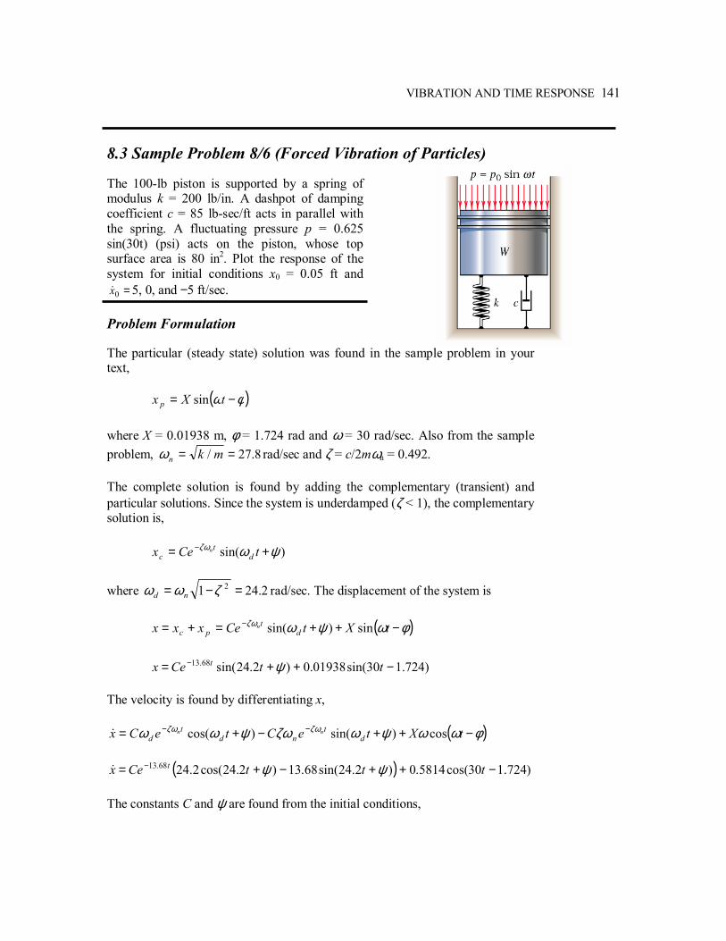
VIBRATION AND TIME RESPONSE 141
8.3 Sample Problem 8/6 (Forced Vibration of Particles) The 100-lb piston is supported by a spring of modulus k = 200 lb/in. A dashpot of damping coefficient c = 85 lb-sec/ft acts in parallel with the spring. A fluctuating pressure p = 0.625 sin(30t) (psi) acts on the piston, whose top surface area is 80 in2. Plot the response of the system for initial conditions x0 = 0.05 ft and
=0x& 5, 0, and −5 ft/sec. Problem Formulation The particular (steady state) solution was found in the sample problem in your text, ( )φω −= tXx p sin where X = 0.01938 m, φ = 1.724 rad and ω = 30 rad/sec. Also from the sample problem, 8.27/ == mknω rad/sec and ζ = c/2mωn = 0.492. The complete solution is found by adding the complementary (transient) and particular solutions. Since the system is underdamped (ζ < 1), the complementary solution is, )sin( ψωζω += − tCex d
tc
n where 2.241 2 =−= ζωω nd rad/sec. The displacement of the system is ( )φωψωζω −++=+= − tXtCexxx d
tpc
n sin)sin( )724.130sin(01938.0)2.24sin(68.13 −++= − ttCex t ψ The velocity is found by differentiating x,
( )φωωψωζωψωω ζωζω −++−+= −− tXteCteCx dt
ndt
dnn cos)sin()cos(&
( ) )724.130cos(5814.0)2.24sin(68.13)2.24cos(2.2468.13 −++−+= − tttCex t ψψ&
The constants C and ψ are found from the initial conditions,
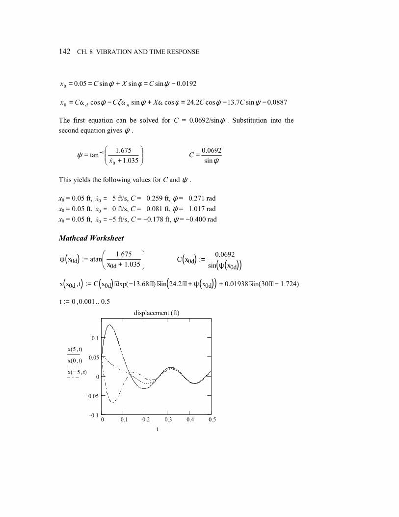
142 CH. 8 VIBRATION AND TIME RESPONSE
0192.0sinsinsin05.00 −=+== ψφψ CXCx
0887.0sin7.13cos2.24cossincos0 −−=+−= ψψφωψζωψω CCXCCx nd&
The first equation can be solved for C = 0.0692/sinψ . Substitution into the second equation gives ψ .
+
= −
035.1675.1tan
0
1
x&ψ
ψsin0692.0=C
This yields the following values for C and ψ . x0 = 0.05 ft, =0x& 5 ft/s, C = 0.259 ft, ψ = 0.271 rad x0 = 0.05 ft, =0x& 0 ft/s, C = 0.081 ft, ψ = 1.017 rad x0 = 0.05 ft, =0x& −5 ft/s, C = −0.178 ft, ψ = −0.400 rad Mathcad Worksheet
ψ x0d( ) atan1.675
x0d 1.035+
:= C x0d( ) 0.0692sin ψ x0d( )( ):=
x x0d t,( ) C x0d( ) exp 13.68− t⋅( )⋅ sin 24.2 t⋅ ψ x0d( )+( )⋅ 0.01938 sin 30 t⋅ 1.724−( )⋅+:= t 0 0.001, 0.5..:=
0 0.1 0.2 0.3 0.4 0.50.1
0.05
0
0.05
0.1
displacement (ft)
x 5 t,( )
x 0 t,( )
x 5− t,( )
t