Solving Inverse Problems withSpectral Data

Joyce R. McLaughlinDepartment of Mathematical Sciences

Rensselaer Polytechnic InstituteTroy, NY 12180mclauj@rpi.edu

Abstract

We consider a two dimensional membrane. The goal is to find propertiesof the membrane or properties of a force on the membrane. The data isnatural frequencies or mode shape measurements. As a result, the functionalrelationship between the data and the solution of our inverse problem is bothindirect and nonlinear. In this paper we describe three distinct approachesto this problem. In the first approach the data is mode shape level setsand frequencies. Here formulas for approximate solutions are given basedon perturbation results. In the second approach the data is frequencies andboundary mode shape measurements; uniqueness results are obtained usingthe boundary control method. In the third approach the data is frequenciesfor four boundary value problems. Local existence, uniqueness results areestablished together with numerical results for approximate solutions.

2

Introduction

We consider two dimensional membranes. Spectral data is measured for thesemembranes; that is natural frequencies and/or some specific measurementsof the corresponding mode shapes. Choices for the mode shape measure-ments are level sets or nodal sets in the interior of the membrane or flux ordisplacement measurements on the boundary. We ask: What can we learnabout the membrane from these measurements?

To obtain this data we excite the membrane at a sequence of natural fre-quencies, often driving the membrane with a time harmonic force at a singlepoint. What results is a wave that travels across the membrane reflectingfrom the boundary, traveling back, reflecting again and so on. At most fre-quencies the initial and reflected waves interfere with each other producinga small response. At a natural frequency the initial and reflected waves rein-force each other producing a large response. This response, a combination oftraveling waves, makes the membrane appear to be oscillating up and down,we call what we see ”a standing wave,” and the shape at any instant of timeis called a mode shape. The shape is the same at all instances except for amultiplicative or amplitude factor.

When, for example, the edge of the membrane is fixed we can measurelevel sets of the mode shape by illuminating the membrane with two lasers.The interference pattern is a set of dark and light lines called a holographicimage. Each line is a level set. Of course one of these level sets is the nodalset, the set of points that don’t vibrate when the membrane is excited at anatural frequency. If, however, we want only the nodal set, a Doppler shiftexperiment may be considered. There, a single laser is used. As it scans themembrane the Doppler shift in the backscatter is measured and minimumDoppler shift is achieved at nodal points. See [McL2] for more discussionabout this.

If, for example, the edge of the membrane is free and our data is displace-ment of the mode shape at the boundary points together with the corre-sponding natural frequencies a third experiment can be considered. We canimpart an impulse at a point on the membrane. Displacement as a responseof the impulse is measured at points around the boundary. We Fourier an-alyze the response at each point and obtain the natural frequencies and thecorresponding displacements at the boundary.

To put these two approaches in perspective we recall what is known inone dimension for Sturm-Liouville problems with separable boundary condi-

3

tions. The classic approach was initially successfully attacked by Borg [B],Gelfand-Levitan [GL], Hochstadt [Ho] and many others for the differentialequation y′′+(λ− q)y = 0 on 0 ≤ x ≤ 1 with separable boundary conditionsand q ∈ L2(0, 1), with a complete solution to the inverse spectral problem forthis equation given by [PT], [IT], [IMT]. These results for the inverse problemrequire two sets of spectral data. In one approach to the problem the data setconsists of two sequences of frequencies each for a different set of separableboundary conditions; another data set is one set of frequencies together withmode shape measurements on the boundary (at x = 0 and 1), that are differ-ent from the boundary conditions. Each data set produces a unique solution;in the work of Trubowitz, et. al., necessary and sufficient conditions that thedata determines q together with the boundary conditions are established. Animportant extension of these results is given in [CMcL1], [CMcL2] where nec-essary and sufficient conditions, together with formulas for exact solutions,for the inverse spectral problem for (py′)′ + λpy = 0, p > 0, p ∈ H1(0, 1)and with Dirichlet boundary conditions are established. This equation can-not be transformed to the one given above with q. For that transformation,p ∈ H2(0, 1) is needed. Note that the weakening of the smoothness prop-erties of p are important for applications. In fact for applications requiringp to be of bounded variation, i.e. p ∈ BV [0, 1], is often the more realis-tic assumption, especially when the material properties are expected to havediscontinuities. A complete characterization as was established by [PT], [IT],[IMT], for q, and extended by Coleman and McLaughlin [CMcL1], [CMcL2],for p ∈ H1(0, 1), is still an open problem for p ∈ BV [0, 1]. Note, however,that inroads for the p ∈ BV [0, 1] problem have been made by [C], [Ha1],[W1], [W2]. In [Ha2], [Ha3], the author presents an implementation of nu-merical methods intended for geophysical applications. See also [HMcL4] fornew results on the asymptotic behavior of eigenvalues in the BV case.

In a second approach for solving the one dimensional inverse spectralproblem, the data is natural frequencies and level set measurements for thecorresponding mode shapes. Sufficient conditions for a unique q ∈ L2(0, 1)are given in [McL1]. Sufficient conditions for a unique p, ρ ∈ H2(0, 1), for(py′)′ + λρy = 0 with separable boundary conditions or an even smootherpair are given in [HMcL2], [HMcL3]. In [HMcL3] numerical implementationof algorithms, that calculate an approximation to one coefficient when theothers are known, and that require a natural frequency together with levelset measurements from a single mode shape, are given. Error bounds forthe difference between the computed approximation and the true solution

4

are established. For these computations, the zero level set, or nodal set, isthe one that is used. This work is extended to p, ρ ∈ BV [0, L] in [HMcL4](with a significant advance using number theory on the asymptotic behaviorof the frequencies). Note that in all cases considered in [HMcL2], [HMcL3],[HMcL4] the algorithms produce piecewise constant approximates; each con-stant is the difference or ratio of the squares of two frequencies. One of thefrequencies is measured and the other is calculated by a very simple formulausing only adjacent zero level set data, or adjacent nodes.

This second one-dimensional approach using the zero level set data isextended by [ST], [S], [LY], [LSY]. There new algorithms for q are given andthe smoothness of q is established from the actual positions of the zero levelset data.

The mathematics for solving two dimensional inverse spectral problemshas developed along a number of fronts. Some of the resultant theorems areremarkably similar to the one dimensional results; the techniques however arenew. In all cases new results for the direct problem are required. In one case,described in the first section of this paper, perturbation methods are used.Here for the direct problem, perturbation expansions for almost all naturalfrequencies and mode shapes are developed. In the work completed to dateby McLaughlin, Hald, Lee, and Portnoy, [HMcL1], [LMcL], [McLP], [McL3],a rectangular membrane is considered. The goal is to find the (nonconstant)density or a (nonconstant) coefficient in a restoring force. The problem isdifficult because even when there is no restoring force and the density isconstant the spacing of the eigenvalues, the squares of the natural frequencies,is very irregular, even when all the frequencies are distinct. Some eigenvaluesare well-spaced relative to their neighbors while others are clustered together.Perturbation expansions are established when, in the no restoring force -constant density case at least two conditions are satisfied:

1. There is a bound, which decreases as the frequency increases, on thedistance to the adjacent frequencies;

2. The distance to selected frequencies is large and increasing as the fre-quency increases. The selected frequencies have corresponding modeshapes with similar oscillation properties.

Number theory and analysis are used to establish these results. Further, a2,the square of the ratio of the sides has favorable number theoretic properties;it is irrational and satisfies a Diophantine condition. This aids us to establish

5

the spacing properties above and allows us to write down specific a2, e.g.√

2or√

5, where our analysis holds.The hard work to obtain the perturbation expansions pays off. It is

applied to the case where the data is a natural frequency and level set mea-surements of the mode shape. With this data, simple formulas are obtainedfor the coefficient, q, in the restoring force. In one formula the value of q atselected points is approximated by the difference of two eigenvalues; one ismeasured, the other is calculated from the data near the selected point. Thisformula generalizes to two dimensions a corresponding one-dimensional for-mula. In another formula, q is approximated at selected points by four datapoints chosen near the selected point. There is no one-dimensional counter-part of this formula, see [HMcL3], [McL3], [McL4]. For each formula errorestimates for the difference between q and its approximate value are given.

Even for this data set, which is the eigenfrequency plus the level setmeasurements, it’s possible to eliminate the extensive mathematics neededfor the perturbation results if the error bounds are given in terms of additionaldisplacement measurements. The implementation of such an algorithm isgiven in [LMcL]. The algorithm produces a piecewise constant approximationto the density ρ. Similar to the one-dimensional problem, each constant isthe ratio of two frequencies, one that is measured and one that is calculatedfrom zero level set data measured in the neighborhood where that constantapproximates ρ.

Note that in all of these solutions the formulas yield local information;i.e. if the solution is required in only part of the membrane, level set dataneed only be measured in the same region. The convergence of the piecewiseconstant approximates yields the uniqueness result for q when the domain isa rectangle.

Fewer results have been established when the data, natural frequenciesand level set measurements, are given for domains other than rectangularmembranes. In [G], however, it is shown that in the q identically equal tozero case, when the domain is a circular disk, if all the nodal lines for allnatural frequencies are the same as for the ρ equal constant case, then ρ canonly be a constant.

We turn now to other data sets for the two dimensional inverse spectralproblem. Both kinds of data sets are suggested by analogous one dimensionalinverse problems. For one set of results the data is the eigenfrequencies plusboundary measurements. The boundary measurements, together with theboundary condition, yield full Cauchy data on the boundary of the domain

6

for each eigenfunction. Uniqueness results, see [NSU], [KK], are known andin one case error bounds have been established, see [AS], when only partialdata or noisy data is given. Two very different approaches are applied toachieve results. In one approach the spectral data is shown to be sufficientto define the Dirichlet to Neumann, DtN, map. Then properties of the DtNmaps are used to establish the uniqueness and error bound results, see [NSU]and [AS]. In the second approach, the model for the membrane is muchmore general. The proofs do not depend on perturbation results but use theboundary control method of Belishev [Be1], [Be2]. The allowable models aredivided into classes defined by groups of gauge transformations. A singleelement in each class of models is determined by the spectral data. Thisnonuniqueness when the model class is more general is also seen for one-dimensional problems. These results are described in the second sectionof this paper. Note that, so far, no numerical algorithms and numericalcomputations, using this two dimensional data set, have been presented inthe literature.

The final inverse spectral problem discussed in this paper uses only eigen-values as data for the inverse problem. The conjecture is that if there is asingle unknown coefficient in the membrane model then the eigenvalues forfour eigenvalue problems, each with distinct but related boundary conditions,are enough to determine the unknown coefficient. The last section of this pa-per describes existence, uniqueness results when the unknown coefficient isclose to a constant, is in a finite dimensional space, the domain is a rectan-gle, and the data is a finite number of eigenvalues. Results from numericalreconstruction in two separate cases (one for q and one for ρ) using this data,are given. This discussion is presented in the last section of this paper.

The inverse spectral problem-using frequency

and level set data

We concentrate here on two dimensional results. Under the assumption thatthe motion of the vibrating membrane is time harmonic we concentrate onthe resultant elliptic equation with Dirichlet boundary conditions

−T4u + qu = λρu, x∼ ∈ R, (1)

u = 0, x∼ ∈ ∂R. (2)

7

where R = [0, π/a] × [0, π] and the eigenvalue λ = ω2 were ω is the naturalfrequency. Here T is the (constant) tension, q is the (often nonconstant)amplitude of a restoring force and ρ is the (often nonconstant) density perunit area. The two inverse problems we will consider in this section are: (1)recover q/T when ρ/T is a known constant; or (2) recover ρ/T when q/Tis identically zero. Note that in one dimension, with enough smoothness,using the Liouville change of variables (see, [BR]) these problems can betransformed one to the other. In two dimensions this is not the case.

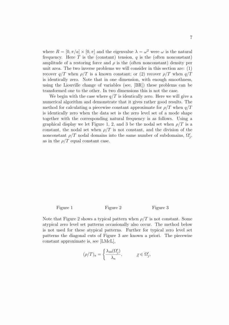
We begin with the case where q/T is identically zero. Here we will give anumerical algorithm and demonstrate that it gives rather good results. Themethod for calculating a piecewise constant approximate for ρ/T when q/Tis identically zero when the data set is the zero level set of a mode shapetogether with the corresponding natural frequency is as follows. Using agraphical display we let Figure 1, 2, and 3 be the nodal set when ρ/T is aconstant, the nodal set when ρ/T is not constant, and the division of thenonconstant ρ/T nodal domains into the same number of subdomains, Ω′

j,as in the ρ/T equal constant case.

Figure 1 Figure 2 Figure 3

Note that Figure 2 shows a typical pattern when ρ/T is not constant. Someatypical zero level set patterns occasionally also occur. The method belowis not used for these atypical patterns. Further for typical zero level setpatterns the diagonal cuts of Figure 3 are known a priori. The piecewiseconstant approximate is, see [LMcL],

(ρ/T )a =

λ10(Ω

′j)

λn

, x∼ ∈ Ω′j,

8

where λn = (ωn)2 is the square of the natural frequency for the displayedmode shape in Figures 2 and 3 and λ10(Ω

′j) is the smallest eigenvalue for

−4u = λu, x∼ ∈ Ω′j,

u = 0, x∼ ∈ ∂Ω′j.

9

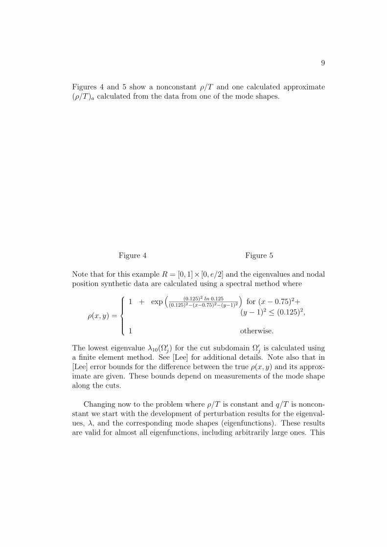
Figures 4 and 5 show a nonconstant ρ/T and one calculated approximate(ρ/T )a calculated from the data from one of the mode shapes.

Figure 4 Figure 5

Note that for this example R = [0, 1]× [0, e/2] and the eigenvalues and nodalposition synthetic data are calculated using a spectral method where

ρ(x, y) =

1 + exp(

(0.125)2 ln 0.125(0.125)2−(x−0.75)2−(y−1)2

)for (x− 0.75)2+

(y − 1)2 ≤ (0.125)2,

1 otherwise.

The lowest eigenvalue λ10(Ω′j) for the cut subdomain Ω′

j is calculated usinga finite element method. See [Lee] for additional details. Note also that in[Lee] error bounds for the difference between the true ρ(x, y) and its approx-imate are given. These bounds depend on measurements of the mode shapealong the cuts.

Changing now to the problem where ρ/T is constant and q/T is noncon-stant we start with the development of perturbation results for the eigenval-ues, λ, and the corresponding mode shapes (eigenfunctions). These resultsare valid for almost all eigenfunctions, including arbitrarily large ones. This

10

job, which is more or less straight forward in one dimension, is made moredifficult by the fact that the eigenvalues in two dimensions, which are real,are on average equally spaced but in actual fact are quite irregularly spacedon the real line. Further under sufficient smoothness assumptions on q/T wecan show that the biggest change in the mode shape, and hence change inthe mode shape level sets, due to a change from constant q/T to nonconstantq/T is made from an interaction with other mode shapes with similar oscil-lation properties. In addition the eigenvalues corresponding to those modeshapes with similar oscillation properties are not the nearest neighbors onthe number line.

To make this more clear we begin now to state some of the hypotheses.The first goal will be to establish results for the spacing of the eigenvalueswhen q/T is identically zero and ρ/T is a constant where we absorb the con-stant into the eigenvalues creating a normalization of ρ/T , that is ρ/T ≡ 1.Further from now on we’ll simply relabel q/T as q. Second we make a choicefor a2; it will be irrational so that all eigenvalues are distinct and satisfy aDiophantine condition. The latter hypothesis allows the utilization of num-ber theoretic arguments in the proofs, considerably shortening the argumentsand further allows, because of a fundamental result of Roth [R], that specifica2, in particular algebraic numbers, can be given for which the theory holds.Specifically the condition required is

The Diophantine Condition:Let J = (1, a0) and 0 < ε0 < 2 be given. Let Z be the set of integers and define

V = a ∈ J | there exists 0 < δ < ε0/6 and K > 0 such that for all p, q ∈Z

with q > 0 :| a2 − p/q |> K/q2+δ

.

Then V is of full measure in J.Examples of numbers that don’t satisfy this condition are given in [HMcL1].

With this assumption the eigenvalue problem

−4u = λu, x∼ ∈ R, (3)

u = 0, x∼ ∈ ∂R, (4)

is considered; it has eigenvalue, (normalized) eigenfunction pairs

λα0 = a2n2 + m2,

11

uα0 =2√

a

πsin anx sin my,

for each α = (an,m), n,m positive integers. Notice that α is an element ina lattice plane L = α = (an, m) | n,m > 0, n, m ∈ Z while λα0 =|α |2 is apoint on the real line. Requiring spacing properties for λα0 on the numberline, sometimes relative to the position of the corresponding α in the latticeplane, is an essential part in the perturbation expansion. Specifically it isestablished that

Lemma 1:For 0 < δ < ε0/6, and a2 satisfying the Diophantine condition, that isa2 ∈ V, the set

M10(a) = α ∈ L | there exists β ∈ L, β 6= α, || α |2 − | β |2 |< 4 | α |−ε0

satisfies

limr→0

#M10(a) ∩ α ∈ L | | α | < r# α ∈ L | | α | < r = 0.

That is M10(a) has density zero in L.

Note that this lemma says that for almost all α ∈ L there is a lower bound,that slowly decreases as | α | gets large, on the distance from λα0 =| α |2 tothe nearest neighbor, λβ0 =| β |2 . This is illustrated in the graph in Figure6.

Figure 6

The second spacing lemma is:

12

Lemma 2:For 0 < ε1 + 5δ + ε1δ < ε2 < 1

2, C1, C2 ≥ 1 and a2 ∈ V, the set

M11(a) = α ∈ L | there exists β ∈ L, with β 6= α, and| α− β | < C1 | α |ε1 ,| λα0 − λβ0 | < C2 | α |1−ε2

has density zero in L, that is

limr→∞

# α ∈ M11(a) | | α | < r# α ∈ L | | α | < r = 0.

This lemma establishes the fact that for almost all α, the lattice points β,that are near α in the lattice plane, and so have the property that the corre-sponding mode shapes uα0, uβ0 have similar oscillation properties, also havethe property that λα0 = |α |2 and λβ0 = |β |2 are a large distance apart onthe number line. A graphical illustration of this is in Figure 7.

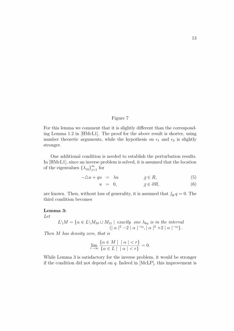
13

Figure 7

For this lemma we comment that it is slightly different than the correspond-ing Lemma 1.2 in [HMcL1]. The proof for the above result is shorter, usingnumber theoretic arguments, while the hypothesis on ε1 and ε2 is slightlystronger.

One additional condition is needed to establish the perturbation results.In [HMcL1], since an inverse problem is solved, it is assumed that the locationof the eigenvalues λjq∞j=1 for

−4u + qu = λu x∼ ∈ R, (5)

u = 0, x∼ ∈ ∂R, (6)

are known. Then, without loss of generality, it is assumed that∫R q = 0. The

third condition becomes

Lemma 3:Let

L\M = α ∈ L\M10 ∪M11 | exactly one λkq is in the interval(| α |2 −2 | α |−ε0 , | α |2 +2 | α |−ε0 .

Then M has density zero, that is

limr→∞

α ∈ M | | α | < rα ∈ L | | α | < r = 0.

While Lemma 3 is satisfactory for the inverse problem, it would be strongerif the condition did not depend on q. Indeed in [McLP], this improvement is

14

accomplished. The alternate lemma is:

Lemma 3A:Let 0 < ε0 < (ε2 − ε1)/2, 0 < ε3 < ε2 − ε1 − 2ε0. Let a ∈ V. Define

M13(a) = α ∈ L\M10 | there exists β, γ ∈ L, β, γ 6= α,0 < | β − γ | < C1 | α |ε1 ,| λβ0 − λα0 | | λγ0 − λα0 |< C3 | α |ε3 .

Then M13 has density zero. Further if M = M10 ∪M11 ∪M13 then M is ofdensity zero in L.

Note that when α ∈ L\M10 ∪M11,∪M13, then it is proved that α ∈ L\M.

Finally the smoothness condition for q is given in terms of

| q |`=

∑

α∈L′| α |2`| aα |2

1/2

where L′ = α = (an,m) | n,m ≥ 0, n, m ∈ Z, where aα are the Fouriercoefficients for q for the basis vα = cα cos (anx) cos my, α ∈ L′, and where

cα =

2√

aπ

if n 6= 0, m 6= 0

√2aπ

if n = 0, m 6= 0 or n 6= 0, m = 0

√a

πif n = 0, m = 0

The precise conditions on `, C1, C2 and C3 are given in [HMcL1], [McLP],as well as the perturbation expansions. Note that for each α ∈ L\M , orα ∈ L\M , there is a unique eigenvalue, eigenfunction pair λαq, uαq that isa perturbation of λα0, uα0. Further, in [HMcL1] the exact error estimatesneeded for the inverse problem solution are derived while in [McLP] a fullperturbation series is established.

Turning now to the solution of the inverse problem, formulas are given inthe following three theorems. To frame the first result we show graphicallyhow we subdivide the membrane. When α ∈ L\M (or α ∈ L\M) satisfiesour conditions, the zero level set for uα0 and the zero level set for uαq, when q

15

is not identically zero, are shown in Figures 8 and 9; in Figure 10 we show thesubdivision of the domain into nm subregions Ω′

j using the zero level set inFigure 9 and diagonal straight line cuts. The straight lines for the diagonalcuts are known apriori and are described in [HMcL1]. Notice the similaritywith the Figures 1, 2 and 3.

Figure 8 Figure 9 Figure 10

Then we form the piecewise constant approximate qa

qa =λαq − λ10(Ω

′j) x∼ ∈ Ω′

j, j = 1, ..., nm

where λ10(Ω′j) is the smallest eigenvalue for

−4u = λu, x∼ ∈ Ω′j,

u = 0, x∼ ∈ ∂Ω′j,

j = 1, 2, ...,m. Then it is proved that,

Theorem 1:Let α ∈ L\M (or α ∈ L\M). Then in each Ω′

j, j = 1, 2, ..., nm there existsan x′j with

| q(x′j)− qα(x′j) |<1

9 | α |2−4α2.

The error estimate in Theorem 1 is valid even when∫R q 6= 0. Note that

similar results have been obtained, see [VA], when the Dirichlet boundaryconditions are replaced by mixed boundary conditions.

16

While this is an elegant formula, extensive numerical computations maybe needed to compute each λ10(Ω

′j) to obtain qα(x′j). Surprisingly, we can

simplify this a great deal. Again we show the idea graphically. In Figure11 we repeat Figure 8 adding the dashed midlines; in Figure 12 we repeatFigure 9 adding the midlines of Figure 11.

Figure 11 Figure 12

Again approximate q by a piecewise constant function but now there is a newformula for the approximate qaa

qaa =λαq − 3λα0 − 2

π[(an)3`x + m3`y], x∼ ∈ Ωj ,

j = 1, ..., nm, where Ωj is any subdomain in Figure 8 (or 11) and `x and `y

are chosen for the same subdomain. Note that the calculation here is verystraight forward requiring only simple differences of the measured data. Tochoose the lengths `x and `y let x′′j be the point of intersection of the dashedmidlines in Ωj. Then `y is the length of the vertical dashed midline passingthrough x′′j and measured from the closest nodal point below x′′j to the closestnodal point above x′′j . The length `x is the corresponding horizontal distance.We can establish

Theorem 2:Let α ∈ L\M(or α ∈ L\M). Then there exists a constant C with

| q (x′′j ) − qaa(x′′j ) | ≤ C | α |−2+(3/2)ε2 .

Finally there are several similar formulas we can establish using nonzero level

17

sets. We give only one here again using a graphical representation. Figure13 shows a non zero level set.

Figure 13

The piecewise constant approximate

qaaa = λαq − 3λα0 + 2((an)22xe + m22ye

)

+2

π

((an)3`e

x + m3`ey

)x∼ ∈ Ωj,

where xe and ye are given apriori and do not depend on the data; errorbounds for q− qaaa at x′′j , similar to those in Theorem 2, can be established,see [McL4].

The inverse spectral problem-using boundary,

spectral data

In this section we briefly review results for inverse spectral problems wherethe data is eigenvalues and boundary data for the eigenmodes. The boundarydata is chosen so that full Cauchy data is known for the eigenmodes on theentire boundary of the region. Two approaches for establishing results havebeen used. In one approach, see [NSU], the spectral data is shown to establishthe Dirichlet to Neumann (DtN) map and then results for DtN maps areused to achieve results. This is a clever use of existing results. Further animportant estimate of the error, see [AS], when only partial spectral data

18

is known and when the data may contain an order ε error is established.A second approach yielding an extensive set of results, see e.g. [BK] and[KK], and relies on the boundary control method first put forth by Belishev,[Be1], for isotropic inverse problems. This work has required the developmentof significant new mathematics and has been generalized to mathematicalmodels that can include anisotropy.

Note that the full set of data considered here, eigenvalues plus boundarydata is more than is needed to achieve a solution to the inverse problem. Therichness of this data is evident in the fact that a full matrix of coefficientswhich could represent anisotropy in a physical medium can be determinedby the data, even when a finite number of eigenvalues and the boundaryeigenmode data for the corresponding eigenmodes is omitted. Note also, insome cases it is possible to use only partial data on the boundary. We do notgive these results here but refer the reader to [Be2, p. R39] for a discussion.

Here we restrict the statement of results to two dimensions even thoughthe original statements of the theorems are stated for dimension n ≥ 2. Webegin by quoting one of the first results in [NSU].

Theorem 3:Let Ω be a bounded domain in R2 with smooth boundary. Let qi ∈ L∞(Ω), i =1, 2, and consider the eigenvalue problems

−∆u + qiu = µu, x∼ ∈ Ω,

u = 0, x∼ ∈ ∂Ω

Denote µj(qi), φj(x; qi)∞j=1 as the eigenvalue, eigenfunction pairs for theabove eigenvalue problems, i = 1, 2, and suppose that

µj(q1) = µj(q2), j = 1, 2, . . . ,

∂φj(x; q1)

∂ν=

∂φj(x; q2)

∂ν, j = 1, 2, . . . , x∼ ∈ ∂Ω

where ν is the unit outward normal to ∂Ω. Then q1(x) = q2(x) for all x ∈ Ω.

Note that although the statement of the above theorem has a Dirichlet bound-ary condition in the eigenvalue problem, this condition is not necessary forthe result; the boundary condition can be changed to ∂u/∂ν + αu = 0 forx∼ ∈ ∂Ω and α a smooth real function in ∂Ω. In this latter case the condition

19

∂φj(x; q1)/∂ν = ∂φj(x; q2)/∂ν for x ∈ ∂Ω is changed to φj(x; q1) = φj(x; q2)for x ∈ ∂Ω, j = 1, 2, . . . With these changes, the conclusion of the theorem isunchanged.

Uniqueness results suggest that stability results can follow. Such resultsare established in [AS] where the main theorem is (again stated only for twodimensions)

Theorem 4:Let Ω be a bounded domain in R2 with smooth boundary. Let qi, i = 1, 2 bebounded Holder continuous functions in Ω with

‖qi‖L∞(Ω) ≤ M,

| qi( x∼)− qi( y∼) |≤ E | x∼− y∼ |α, x∼, y∼ ∈ Ω

for some M, E > 0 and 0 < α < 1. Let λij, φj(x; qi)∞j=1, be the eigenvalue,

eigenfunction pairs for−∆u + qiu = µu, x∼ ∈ Ω,

u = 0, x∼ ∈ ∂Ω,

i = 1, 2. Then there exist positive constants A,B, C and 0 < σ < 1 such thatfor every N > 0,

‖q1 − q2‖L∞(Ω) ≤ C(NAεσ + N−B),

where

ε = supj≤N

| λ1j − λ2

j | + supj≤N

∣∣∣∣∣

∣∣∣∣∣∂φj(x; q1)

∂ν− ∂φj(x; q2)

∂ν

∣∣∣∣∣

∣∣∣∣∣L∞(∂Ω)

.

The authors point out that if the eigenfunctions are not chosen carefully inthe multiple eigenvalue case then it is possible to have ε > 0 even whenq1 ≡ q2. Note also that the constants A,B and σ in the theorem depend onlyon the Holder constant α and the space dimension. The proof of this resultexploits the connection with the DtN map.

We turn now to another set of results where the mathematics that pro-vides the proofs of these results is based in differential geometry. Instead,then, of speaking about anisotropic media, the authors of these results speakabout a compact, connected, oriented differentiable (C∞) manifold, M , withdim M = 2 (again we restrict our statements to two dimensions) and smooth

20

non-zero (one) dimensional manifold boundary S = ∂M . The Riemannianmetric is denoted by g on M with associated measure dV = dVg. What isconsidered then is the operator

Au = a(x,D)u = −g1/2

(∂

∂xk

+ ibk

) (g1/2gk`µ

(∂

∂x`

+ ib`

)u

)+ qu, (7)

where a sum over k and ` is understood implicitly. Note that the metrictensor (gk`)k,`,=1,2 is symmetric,

g(x) = det[gk`]−1, dVg = g1/2dx1dx2,

and µ > 0, with q, bj, j = 1, 2, being real valued and C∞ smooth, andbj, j = 1, 2 forming a differential 1 - form on M . The above operator isconsidered together with the boundary condition

Bu =

(∂

∂ν+ ib · ν + σ

)u = 0, x∼ ∈ S, (8)

where σ is a real valued smooth function defined on S.

The goal of the inverse problem is to recover the coefficients in A and Bfrom incomplete boundary spectral data (IBSD) defined as follows:

Definition:Let N be the set of positive integers and K ′ ⊂ N be a finite subset. Letλk, φkk∈N be the eigenvalue, eigenfunction pairs for

Au = λu, on M,Bu = 0 on S.

(9)

Then the collection (S, λkk∈N−K′ , φk |Sk∈N−K′) is called the incompleteboundary spectral data (IBSD) for the operator A (together with B).

Optimistically one might expect that the IBSD would determine all thecoefficients in A and B but such is not the case. It happens that there isa set of transformations that leave the eigenvalues fixed, that multiply eacheigenfunction on the boundary by the same function, that leave the manifoldunchanged but change A and B; this is the group G of generalized gauge

21

transformations. In any orbit of G, see[KK], there is a unique canonical rep-resentation called the Schrodinger operator (with magnetic potential) (see[KK]). The uniqueness result that can then be obtained is (without specifi-cally defining the canonical Schrodinger operator explicitly) is

Theorem 5:Let A together with B be a canonical Schrodinger operator. Then its IBSD(S, λkk∈N−K′ , φk |sk∈N−K′) determines A and B, i.e. (M, g), q, σ, and buniquely.

The proof, which is quite extensive, does not rely on perturbation methods.Rather detailed results about Gaussian beams, which are rapidly oscillatingsolutions of Au(x, t)+ ∂2

∂t2u(x, t) = 0, concentrated near a space-time ray, are

needed to recover coefficients, such as q, which have a low order effect on thespectral data.

Note that the need to restrict to a canonical problem in order to achieveuniqueness is mirrored in one dimension. There the situation is this. Weconsider the eigenvalue problem

(pux)− q + λρu = 0, 0 < x < 1,(ux + au) |x=0 = 0, (ux + bu) |x=1 = 0,

(10)

where pxx, ρxx, q ∈ L2(0, 1), p, ρ > 0. Then multiply λ by a constant and

divide ρ by the same constant so that the resultant p, ρ satisfy∫ 10

√ρ/pdx = 1.

Following that make the change of dependent and independent variables (theLiouville transformation)

s =∫ x

0

√ρ/pdx,

v = (pρ)1/4u,

to obtain that v satisfies the equations

vss − ((q/ρ) + [((pρ)1/4)ss/(pρ)1/4])v + λv = 0, 0 < s < 1,

(vs

√ρ/p + av) |s=0, (vs

√ρ/p + bv) |s=1 = 0.

(11)

The boundary spectral data becomes

λj, vj(0), vj(1)∞j=1

22

whereλj, vj∞j=1 are the eigenvalue, eigenfunction pairs for (11). Since eachvj can be multiplied by a constant, the information content in vj(0) and vj(1)is contained in vj(1)/vj(0). It is known see e.g. [IT], [IMT] that the data

λj, vj(1)/vj(0)∞j=1

is exactly the right amount of data to uniquely determine the triple

a

b

q(s)

=

a/√

ρ/p(0)

b/√

ρ/p(1)

(q/ρ) + [((pρ)1/4)ss/(pρ)1/4]

(12)

It is not possible, however, to recover the three functions q, p, ρ from (12)uniquely. In fact there is a whole class of Liouville transformations that couldbe applied to obtain problems of the form (10) from the given data. Threepossibilities include:

(I) p, ρ ≡ 1, s = x, a = a, b = b, q = q;

(II) q = cρ with c < minj λj, p ≡ ρ, s = x, a = a, b = b, and p is apositive

solution of (p1/2)ss − (q − c)p1/2 = 0;

(III) q ≡ c < minj λj, ρ ≡ 1, with p a positive solution of

(p1/4)ss − (q − c)p1/4 = 0, satisfying∫ 10

√p(s)ds = 1 and the original

independent variable x =∫ s0

√p(s)ds, also a = a

√p(0), b = b

√p(1).

The inverse spectral problem-using only eigen-

values

It is important to include one more set of results and these results addressthe problem where one recovers material properties using only eigenvalues.To address this challenging problem we first recall that, in one dimension,

23

if we know the eigenvalues for the following two problems, with the sameq ∈ L2(0, 1/2),

y′′ + (λ− q)y = 0 0 < x <1

2(13)

y(0) = y(1

2) = 0

with eigenvalues λ1, λ2, ... and

z′′ + (µ− q)z = 0 0 < x <1

2(14)

z(0) = z′(1

2) = 0

with eigenvalues µ1, µ2, ...

then there is at most one q ∈ L2(0, 1/2) with these sets of eigenvalues. Thiscan be established in a straight forward manner from the results in [PT] andis addressed in [L]. It is also equivalent to the following. First extend q toqe, defined on 0 < x < 1, by making an even reflection of q about x = 1/2.Then the combined set λi∞i=1 ∪ µi∞i=1 is the set of eigenvalues for

w′′ + (η − qe)w = 0, 0 < x < 1, (15)

w(0) = w(1) = 0.

An independent proof for (15), see [PT], shows that there is at most onesymmetric qe ∈ L2(0, 1) for which the combined set λi∞i=1 ,∪µi∞i=1 arethe eigenvalues of (15).

These one dimensional results suggest two related two dimensional in-verse spectral problems. The basic idea is this. If in one dimension twosets of eigenvalues provide a uniqueness result for a nonsymmetric q thenare four sets of eigenvalues enough to provide a uniqueness result in two di-mensions? To illustrate, consider the following example. Let R be the rect-angle R = [0, π/2a] × [0, π/2] with ∂1R = (π/2a, y) | y ∈ [0, π/2] , ∂2R =(x, π/2) | x ∈ [0, π/2a] , ∂3R = (0, y) | y ∈ [0, π/2] and ∂4R = (x, 0) | x ∈ [0, π/2a]subsets of ∂R. Consider the four eigenvalue problems with the same q ∈L∞(R) and n∼ the unit outward normal to points on the ∂R :

4u + (λ− q)u = 0, x∼ ∈ R, (16)

u = 0, x∼ ∈ ∂R,

24

with eigenvalues λ1 < λ2 ≤ λ3 ≤ ...,

4u + (λ− q)u = 0, x∼ ∈ R, (17)

u = 0, x∼ ∈ ∂1R ∪ ∂3R ∪ ∂4R,

5u · n∼ = uy = 0 x∼ ∈ ∂2R,

with eigenvalues µ1 < µ2 ≤ µ3 ≤ ...,

4u + (ν − q)u = 0 x∼ ∈ R, (18)

u = 0 x∼ ∈ ∂2R ∪ ∂3R ∪ ∂4R,

5u · n∼ = ux = 0, x∼ ∈ ∂1R,

with eigenvalues ν1 < ν2 ≤ ν3 ≤ ..., and

4u + (η − q)u = 0, x∼ ∈ R, (19)

u = 0, x∼ ∈ ∂3R ∪ ∂4R,

5u · n∼ = 0 x∼ ∈ ∂1R ∪ ∂2R,

with eigenvalues η1 < η2 ≤ η3 ≤ ...

By evenly reflecting q about ∂1R and then evenly reflecting the resultant qabout the resultant extension of ∂2R then we obtain the eigenvalue problem

4u + (λ− qe)u = 0, x∼ ∈ R = [0, π/a]× [0, π], (20)

u = 0, x∼ ∈ ∂R,

with eigenvalues λi∞i=1 ∪ µi∞i=1 ∪ νi∞i=1 ∪ ηi∞i=1 and where qe is theeven extension of q to all of R. Hence for this particular problem, solving theinverse problem of finding a symmetric qe ∈ L∞(R) from the eigenvalues of(20) is equivalent to finding a nonsymmetric q ∈ L∞(R) from the eigenvaluesof (16), (17), (18), (19).

To illustrate the known results then we consider only (20) and a relatedproblem

1

λ4 u + ρu = 0, x∼ ∈ R, (21)

u = 0, x∼ ∈ ∂R,

25

where in this related problem the goal is to solve the inverse problem: find asymmetric ρ > 0 from the eigenvalues of (21).

Two local results are known. Both produce functions q or ρ for which (20),or respectively (21), have a given finite number, say m, eigenvalues. Bothextended a method first developed by Hald, [Ha1], for the one dimensionalinverse spectral problem. The basic idea is to establish an approximate ma-trix eigenvalue problem for (20) (and similarly (21)) where the approximateproblem is derived using spectral approximations. For each matrix prob-lem q (or ρ) is assumed to be in the span of m given basis functions andeach eigenfunction is in the span of N (possibly different) basis functions,N ≥ m. With m fixed for each N a function qN (or ρN is determined as asolution of the corresponding N ×N matrix inverse eigenvalue problem. AsN →∞, qN → q (or ρN → ρ) a function in the span of the m basis functions.For that q or ρ the eigenvalue problem (20) (and similarly (21)) has the givenfinite set of eigenvalues.

Specifically in [KMcL] and [McC], the following are proved. For (20),

Theorem 6:Let

λ0

n

m

n=1= Λ0 be the first m eigenvalues for

4u + λu = 0, x∼ ∈ R,

u = 0, x∼ ∈ ∂R,

with R = [0, π/a] × [0, π], a > 0 and with min1≤n 6=n′≤m | λ0n−λ0

n′ |= δ > 0.Let Λ = λnm

n=1 , all distinct, be given along with a set of symmetric, or-thonormal basis functions ψnm

n=1, each symmetric on R. Then there existsδ1, δ2 > 0, βnm

n=1 and symmetric q =∑m

n=1 βnψnwith ‖ Λ− Λ0 ‖`2< δ1,‖ q ‖L∞< δ2 and with the property that Λ = λnm

n=1 are the first m eigen-values of

4u + (λ− q)u = 0, x∼ ∈ R,

u = 0, x∼ ∈ ∂R.

And for (21),

26

Theorem 7:Let

1/λ0

n

m

n=1= Γ0 be the first m eigenvalues for

1

λ4 u + u = 0, x∼ ∈ R,

u = 0, x∼ ∈ ∂R.

with min1≤n 6=n′≤m | 1/λ0n − 1/λ0

n′ |= δ > 0. LetΓ = 1/λnmn=1, all distinct

be given along with a set of symmetric orthonormal basis functions ψnmn=1.

Then there exist δ1, δ2 > 0, βnmn=1, and symmetric ρ = 1 +

∑mn=1 βnψn with

‖ Γ − Γ0 ‖`2< δ1, ‖ ρ − 1 ‖L∞< δ2 such that Γ = 1/λnmn=1 are the first m

eigenvalues for

1

λ4 u + ρu = 0, x∼ ∈ R,

u = 0 x∼ ∈ ∂R.

Note that in [KMcL] and [McC], the constants δ1 and δ2 are given explicitlyin terms of δ. Note also that both theorems are proved using contractionmappings and the same idea is used for the numerical algorithms. Examplesto show achieved results from the numerical computations are contained inFigures 14, 15, 16 and Figure 17. Figure 14 exhibits

q1(x, y) =

exp(

−1d(x,y)

)if d(x, y) = 1− (x− π

2a)2 − 3(y − π

2)2 > 0,

0 otherwise,

with a =√

0.9, used to compute the eigenvalues λn8n=1. The eigenvalues

are calculated using a Matlab finite element package. Figure 15 shows theprojection of q1 onto the span of ψn8

n=1 where each

27

ψn = (2√

a/π) sin((2sn − 1)ax) sin((2tn − 1)y) with (sn, tn) distinct pairs ofintegers for n = 1, ..., 8; Figure 16 exhibits the reconstruction of the approx-imate q1 =

∑8n=1 βnψn using the matrix approximation of (20), the data

λn8n=1 and the resultant fixed point iteration to solve the matrix inverse

problem for βn8n=1 when N = 64.

Figure 14 Figure 15

Figure 16

Figure 17 shows the results of the computation for approximate ρ = 1 +∑10n=1 βnψn in (21) from given Γ = 1/λn10

n=1. Here the eigenvalue data is

28

again calculated with a Matlab finite element tool box and with

ρ =

1 + exp(

−1d(x,t)

)if d(x, y) =

(π3

)2 − 4(x− π

2a

)2 −(y − π

2

)2> 0,

1 otherwise,

and with a =√

0.85.

Note that for this problem (21), new theoretical complications arise partlybecause the effect of changes in ρ on the eigenvalues (and vice-versa) is ratherstrong.

Figure 17

Determining whether four sets of eigenvalues is enough to determine q (or ρ)for general domains, for q (or ρ) in an infinite dimensional space, and for q(or ρ) not sufficiently close to a constant is an open problem.

Acknowledgement

The author is grateful to C. J. Lee, Roger Knobel and Maeve McCarthy forallowing for the inclusion of their numerical calculations in this paper.

29

References

[A] G. Alessandrini, ”Stable Determination of Conductivity by BoundaryMeasurements”, Applicable Analysis, Vol. 27, (1988), pp. 153-172.

[AS] G. Alessandrini and J. Sylvester, ”Stability for a Multidimensional In-verse Spectral Theorem”, Comm. Math. Phys., Vol. 5, No. 5, (1990), pp.711-736.

[Be1] M.I. Belishev, ”On an approach to Multidimensional Inverse Problemsfor the wave equation”, Dokl. Akad. Nauk SSSR (in Russian), Vol. 297, No.3, (1987), pp. 524-527.

[Be2] M.I. Belishev, ”Boundary control in reconstruction of manifolds andmetrics (the BC method),” Inverse Problems, Vol. 13 (1997), No. 5 pp.R1-R45.

[Bo] G. Borg, Eine Umkehrung der Sturm-Liouvilleschen Eigenwertaufgab,Acta Math. Vol. 78, (1946), pp. 1-96.

[BB] V.M. Babich and V.S. Buldyrev, Short-wavelength Diffraction Theory,Springer Verlag, New York, 1991.

[BK] M.J. Belishev and Ya. Kurylev, ”To the Reconstruction of a Rieman-nian Manifold via its Spectral Data (BC-method)”, Comm. P.D.E., Vol. 17,No. 5-6, (1992), pp. 767-804.

[BR] G. Birkhoff and G-C. Rota, Ordinary Differential Equations, Wiley,New York, 1989.

[C] R. Carlson, ”An Inverse Spectral Problem for Sturm-Liouville Operatorswith Discontinuous Coefficients,”Proc. Amer. Math. Soc., Vol. 120, (1994)pp. 475-484.

[CMcL1] C.F. Coleman and J.R. McLaughlin, ”Solution of the Inverse Spec-tral Problem for an Impedance with Integrable Derivative, Part I.” Comm.Pure andAppl. Math., Vol. 46 (1993), pp. 145-184.

30

[CMcL2] C.F. Coleman and J.R. McLaughlin, ”Solution of the Inverse Spec-tral Problem for an Impedance with Integrable Derivative, Part II.” Comm.Pure and Appl. Math., Vol. 46 (1993), pp. 185-212.

[GL] I.M. Gel’fand and B.M. Levitan, ”On the Determination of a Differen-tial Equation from its Spectrum,” Ivz. Akad. Nauk SSSR Ser. Math., Vol.15 (1951), pp. 309-360; Amer. Math. Trans., Vol. 1 (1955), pp. 233-304.

[Ha1] O.H. Hald, ”The Inverse Sturm-Liouville Problem and the Rayleigh-Ritz Method,” Math. Comp., Vol. 32, No. 143, (1978), pp. 687-705.

[Ha2] O. H. Hald, ”Inverse Eigenvalue Problems for the mantle,” GeophysicalJournal of the Royal Astronomical Society, Vol. 62 (1980), pp. 41-48.

[Ha3] O. H. Hald, ”Inverse eigenvalue problems for the mantel-II,” Geophys-ical Journal of the Royal Astronomical Society, Vol. 72 (1983), pp. 139-164.

[Ho] H. Hochstadt, ”The Inverse Sturm Liouville Problem”, CPAM, Vol.XXVI, (1973), pp. 715-729.

[HMcL1] O.H. Hald and J.R. McLaughlin, Inverse Nodal Problems: FindingthePotential from Nodal Lines, AMS Memoir, January 1996.

[HMcL2] O.H. Hald and J.R. McLaughlin, ”Inverse Problems Using NodalPosition Data - Uniqueness Results, Algorithms and Bounds,” Proceedingsof theCentre for Mathematical Analysis, edited by R.S. Anderson and G.N. Newsam,Australian National University, Vol. 17 (1988), pp. 32-59.

[HMcL3] O.H. Hald and J.R. McLaughlin, ”Solutions of Inverse Nodal Prob-lems,” Inverse Problems, Vol. 5 (1989), pp. 307-347.

[HMcL4] O.H. Hald and J.R. McLaughlin, ”Inverse Problems: Recovery ofBV Coefficients from Nodes,” Inverse Problems, Vol. 14 (1998), pp. 245-273.

[IT] E.L. Isaacson and E. Trubowitz, ”The Inverse Sturm-Liouville Problem

31

I,” Comm. Pure and Appl. Math, Vol. 36 (1983), pp. 767-783.

[IMT] E.L. Isaacson, H.P. McKean and E. Trubowitz, ”The Inverse Sturm-Liouville Problem II,” Comm. Pure and Appl. Math. Vol. 36 (1983), pp.767-783.

[KK] A. Katchalov and Ya. Kurylev, ”Multidimensional Inverse Problemwith Incomplete Boundary Spectral Data”, Comm. P.D.E., Vol. 23(1&2),(1998), pp. 55-95.

[KMcL] R. Knobel and J.R. McLaughlin, ”A Reconstruction Method for aTwo-Dimensional Inverse Eigenvalue Problem.” ZAMP, Vol. 45 (1994), pp.794-826.

[L] B. M. Levitan, ”On the determination of a Sturm-Liouville equation bytwo spectra,” Izv. Akad. Nauk, SSSR Ser. Mat. Vol. 28 (1964) pp. 63-78;Amer. Math. Soc. transl. Vol. 68 (1968) pp. 1-20.

[Lee] C. A. Lee, ”An inverse nodal problem of a membrane,” Ph. D. thesis,Rensselaer Polytechnic Institute, 1995.

[LMcL] C.J. Lee and J.R. McLaughlin, ”Finding the Density for a Membranefrom Nodal Lines,”Inverse Problems in Wave Propagation, eds. G. Chavent,G. Papanicolaou, P. Sacks, W.W. Symes, (1997), Springer Verlag, pp. 325-345.

[LSY] C.K. Law, C-L Shen and C-F Yang, ”The Inverse Nodal Problem onthe Smoothness of the Potential Function,” Inverse Problems, Vol. 15 (1999),pp. 253-263.

[LY] C.K. Law and C.F. Yang, ”Reconstructing the Potential Function andits Derivative Using Nodal Data,” Inverse Problems, Vol. 14, (1998), pp.299-312.

[McC] C.M. McCarthy, ”The Inverse Eigenvalue Problem for a WeightedHelmholtz Equations,” (to appear Applicable Analysis).

[McL1] J.R. McLaughlin, ”Inverse Spectral Theory Using Nodal Points as

32

Data - A Uniqueness Result.” J. Diff. Eq., Vol. 73. (1988), pp. 354-362.

[McL2] J.R. McLaughlin, ”Good Vibrations,” American Scientist, Vol. 86,No. 4, July-August (1998), pp. 342-349.

[McL3] J.R. McLaughlin, ”Formulas for Finding Coefficients from Nodes/NodalLines,” Proceedings of the International Congress of Mathematicians,Zurich, Switzerland 1994, Birkhauser Verlag, (1995), pp. 1494-1501.

[McL4] J.R. McLaughlin, ”Using Level Sets of Mode Shapes to Solve InverseProblems.” (to appear).

[McLP] J.R. McLaughlin and A. Portnoy, ”Perturbation Expansions for Eigen-values and Eigenvectors for a Rectangular Membrane Subject to a Restora-tive Force,” Comm. P.D.E., Vol. 23 (1&2), (1998), pp. 243-285.

[NSU] A. Nachman, J. Sylvester and G. Uhlmann, ”An n-Dimensional Borg-Levinson Theorem,” Comm. Math. Phys. Vol. 115, No. 4 (1988), pp.595-605.

[PT] J. Poschel and E. Trubowitz, Inverse Spectral Theory, Academic Press,Orlando, (1987).

[S] C.L. Shen, ”On the Nodal Sets of the Eigenfunctions of the String Equa-tions,” SIAM J. Math. Anal., Vol. 19, (1998), pp. 1419-1424.

[ST] C.L. Shen and T.M. Tsai, ”On Uniform Approximation of the Den-sity Function of a String Equation Using Eigenvalues and Nodal Points andSome Related Inverse Nodal Problems,” Inverse Problems, Vol. 11, (1995),pp. 1113-1123.

[VA ] C. Vetter Alvarez, ”Inverse Nodal Problems with Mixed BoundaryConditions,” Ph. D. thesis, University of California, Berkeley, 1998.