Solving Job Shop Scheduling with Setup Times through ... · Solving Job Shop Scheduling with Setup Times through Constraint-based Iterative Sampling: An Experimental Analysis Angelo

Noname manuscript No.(will be inserted by the editor)

Solving Job Shop Scheduling with Setup Times throughConstraint-based Iterative Sampling: An ExperimentalAnalysis

Angelo Oddi · Riccardo Rasconi ·Amedeo Cesta · Stephen F. Smith

Received: date / Accepted: date

Abstract This paper presents a heuristic algorithm for solving a job-shop scheduling

problem with sequence dependent setup times and min/max separation constraints

among the activities (SDST-JSSP/max). The algorithm relies on a core constraint-

based search procedure, which generates consistent orderings of activities that require

the same resource by incrementally imposing precedence constraints on a temporally

feasible solution. Key to the effectiveness of the search procedure is a conflict sam-

pling method biased toward selection of most critical conflicts and coupled with a

non-deterministic choice heuristic to guide the base conflict resolution process. This

constraint-based search is then embedded within a larger iterative-sampling search

framework to broaden search space coverage and promote solution optimization. The

efficacy of the overall heuristic algorithm is demonstrated empirically both on a set

of previously studied job-shop scheduling benchmark problems with sequence depen-

dent setup times and by introducing a new benchmark with setups and generalized

precedence constraints.

Keywords random-restart · constraint-based reasoning · job-shop scheduling · setup

times · generalized precedence constraints

1 Introduction

This paper describes an approach for solving job-shop scheduling problems with ready

times, deadlines, sequence dependent setup times and min/max separation constraints

among activities (SDST-JSSP/max). Similar problems are common in a semiconduc-

tor manufacturing environment – see Ovacik and Uzsoy (1994, 1997) – and in general,

over the last ten years, there has been an increasing interest in solving scheduling

Angelo Oddi · Riccardo Rasconi · Amedeo CestaInstitute for Cognitive Science and TechnologyItalian National Research Council, Rome, ItalyE-mail: [email protected]

S.F. SmithRobotics Institute, Carnegie Mellon University, Pittsburgh, PA, USAE-mail: [email protected]

2

problems with setup times (Allahverdi and Soroush 2008; Allahverdi et al 2008). This

fact stems mainly from the observation that in many real-word industry or service

environments there are tremendous savings when setup times are explicitly considered

in scheduling decisions.

The algorithm proposed in this work relies on a core constraint-based search proce-

dure, which generates a consistent ordering of activities that require the same resource

by incrementally adding precedence constraints between activity pairs belonging to a

temporally feasible solution. The algorithm bases its solving capability on a general

meta-heuristic which, despite its simplicity, has proven to be quite effective, generat-

ing competitive results for a wide range of different scheduling problems. Specifically,

the algorithm we propose in this work is an extension of the stochastic version of the

sp-pcp procedure proposed in Oddi and Smith (1997) suitable for solving scheduling

problems with setup times. The resulting procedure is then embedded within a larger

iterative-sampling search framework, also used in Cesta et al (2002), to broaden search

space coverage and promote solution optimization.

The main objective of this work is to investigate the generality of this constraint-

based approach and its adaptability to the SDST-JSSP/max, to understand the extent

to which its traditional effectiveness and efficiency is preserved in this setting. In this

regard we show: (1) that the general algorithm can be adapted to the setup times case

with minimal effort and change; and (2) that the solving capabilities of our algorithm

remain unaltered even in the presence of min/max separation constraints. These claims

are substantiated by means of an extensive experimental analysis.

Within the current literature, there are several other examples of procedures for

solving scheduling problems with setup times that are extensions of counterpart pro-

cedures for solving the same (or similar) scheduling problem without setup times. This

is the case of the work by Brucker and Thiele (1996), for example, which relies on

an earlier solutions introduced in Brucker et al (1994). Another example is the more

recent work of Vela et al (2009) and Gonzalez et al (2009a), which proposes effective

heuristic procedures based on genetic algorithms and local search. The local search

procedures that are introduced in these works extend a procedure originally proposed

by Nowicki and Smutnicki (2005) for the classical job-shop scheduling problem to the

setup times case by introducing a neighborhood structure that exhibits similar prop-

erties relatively to critical paths in the underlying disjunctive graph formulation of the

problem. A third example is the work of Balas et al (2008), which extends the well-

know shifting bottleneck procedure (Adams et al 1988) to the SDST-JSSP case. All of

the procedures just mentioned solve a relaxed version of the full SDST-JSSP/max in

which there are no min/max separation constraints (we will refer to this problem in

the following as the SDST-JSSP). Both Balas et al (2008) and Gonzalez et al (2009a)

have produced reference results with their techniques on a previously studied bench-

mark set of SDST-JSSP problems proposed by Ovacik and Uzsoy (1994). Despite our

broader interest in solving the SDST-JSSP/max, we use this benchmark problem set

as a basis for direct comparison to our solution procedure in the experimental section

of this paper.

The procedure we propose is not the only one which relies on the constraint-solving

paradigm; another example is described in (Focacci et al 2000), which introduces a more

elaborate procedure based on the integration of two different solution models. One key

feature of our procedure is its simplicity, in spite of its effectiveness in solving a set of

difficult instances of SDST-JSSPs. The advantages of simplicity will be argued as the

algorithm and the experimental analysis are presented.

3

This paper is organized as follows. An introductory section defines the reference

SDST-JSSP/max problem and its representation. A central section describes the core

constraint-based procedure and the overarching iterative sampling search strategy. An

experimental section describes the performance of our algorithm the benchmark prob-

lem set of well-known SDST-JSSPs and the most interesting results are explained.

Finally, a new set of benchmark problems that captures the full complexity of the

SDST-JSSP/max is introduced. Some conclusions and a discussion of future work

end the paper.

2 The Scheduling Problem with Setup Times

In this section we provide a definition of the job-shop scheduling problem with sequence

dependent setup times which is extended to include min/max separation constraints

(SDST-JSSP/max). To the best of our knowledge, this generalization of the SDST-

JSSP has not been previously considered in the literature. We have selected this rather

complex problem as our focus in this paper principally as a means of better showing

the effectiveness and versatility of our general constraint-based search procedure. Its

effectiveness will be demonstrated by comparing our algorithm’s performance with

current known best known results on the previously studied SDST-JSSP, which is the

relaxed version of the SDST-JSSP/max that excludes time windows. Its versatility

will be established by first showing the original algorithm’s adaptability to the SDST-

JSSP, and then its direct applicability to the extended case when time lags are added

to the problem.

The SDST-JSSP/max entails the synchronization of a set of resources R = {r1, r2,. . . , rm} to perform a set of n activities A = {a1, . . . , an} over time. The set of activities

is partitioned into a set of nj jobs J = {J1, . . . , Jnj}. The processing of a job Jkrequires the execution of a strict sequence of m activities aik ∈ Jk (i = 1, . . . ,m), and

the execution of each activity aik is subject to the following constraints:

– resource availability - each activity ai requires the exclusive use of a single resource

rai for its entire duration; no preemption is allowed and all the activities included

in a job Jk require distinct resources.

– processing time constraints - each ai has a fixed processing time pi such that ei −si = pi, where the variables si and ei represent the start and end time of ai.

– separation constraints - for each pair of successive activities aik and a(i+1)k in a

job Jk, there is a min/max separation constraint lminik ≤ s(i+1)k − eik ≤ lmax

ik ,

i = 1, . . . ,m− 1.

– sequence dependent setup times - for each resource r, the value strij represents the

setup time between two generic activities ai and aj (aj is scheduled immediately

after ai) requiring the same resource r, such that ei + strij ≤ sj . As is traditionally

assumed in the literature, the setup times strij satisfy the so-called triangular in-

equality (see Brucker and Thiele (1996); Artigues and Feillet (2008)). The triangle

inequality states that, for any three activities ai, aj , ak requiring the same resource,

the inequality strij ≤ strik + strkj holds.

– job release and due dates - each Job Jk has a release date rdk, which specifies

the earliest time that any activity in Jk can be started, and a due date dk, which

designates the time by which all activities in Jk should be completed. The due date

is not a mandatory constraint and can be violated (see below).

4

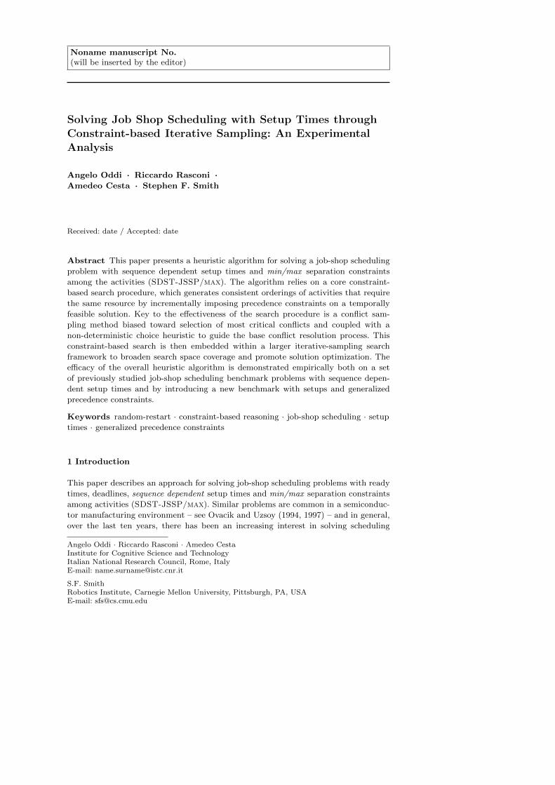
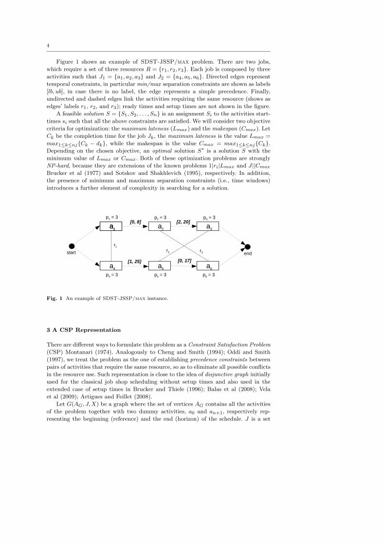
Figure 1 shows an example of SDST-JSSP/max problem. There are two jobs,

which require a set of three resources R = {r1, r2, r3}. Each job is composed by three

activities such that J1 = {a1, a2, a3} and J2 = {a4, a5, a6}. Directed edges represent

temporal constraints, in particular min/max separation constraints are shown as labels

[lb, ub], in case there is no label, the edge represents a simple precedence. Finally,

undirected and dashed edges link the activities requiring the same resource (shows as

edges’ labels r1, r2, and r3); ready times and setup times are not shown in the figure.

A feasible solution S = {S1, S2, . . . , Sn} is an assignment Si to the activities start-

times si such that all the above constraints are satisfied. We will consider two objective

criteria for optimization: the maximum lateness (Lmax) and the makespan (Cmax). Let

Ck be the completion time for the job Jk, the maximum lateness is the value Lmax =

max1≤k≤nj{Ck − dk}, while the makespan is the value Cmax = max1≤k≤nj{Ck}.Depending on the chosen objective, an optimal solution S∗ is a solution S with the

minimum value of Lmax or Cmax. Both of these optimization problems are strongly

NP-hard, because they are extensions of the known problems 1|ri|Lmax and J ||Cmax

Brucker et al (1977) and Sotskov and Shakhlevich (1995), respectively. In addition,

the presence of minimum and maximum separation constraints (i.e., time windows)

introduces a further element of complexity in searching for a solution.

a1 a2 a3

a4 a6a5

[1, 25]

[2, 20][0, 8]p1 = 3 p2 = 3 p3 = 3

p4 = 3 p5 = 3 p6 = 3

a1

[0, 17]

r3r2

r1

start end

Fig. 1 An example of SDST-JSSP/max instance.

3 A CSP Representation

There are different ways to formulate this problem as a Constraint Satisfaction Problem

(CSP) Montanari (1974). Analogously to Cheng and Smith (1994); Oddi and Smith

(1997), we treat the problem as the one of establishing precedence constraints between

pairs of activities that require the same resource, so as to eliminate all possible conflicts

in the resource use. Such representation is close to the idea of disjunctive graph initially

used for the classical job shop scheduling without setup times and also used in the

extended case of setup times in Brucker and Thiele (1996); Balas et al (2008); Vela

et al (2009); Artigues and Feillet (2008).

Let G(AG, J,X) be a graph where the set of vertices AG contains all the activities

of the problem together with two dummy activities, a0 and an+1, respectively rep-

resenting the beginning (reference) and the end (horizon) of the schedule. J is a set

5

of directed edges (ai, aj) representing the precedence constraints among the activities

(job precedence constraints) and are weighted with the processing time pi of the edge’s

source activity ai. The set of undirected edges X represents the disjunctive constraints

among the activities requiring the same resource r. There is an edge for each pair of

activities ai and aj requiring the same resource r and the related label represents the

set of possible ordering between ai and aj : ai � aj or aj � ai.

Hence, in CSP terms, a decision variable xijr is defined for each pair of activities

ai and aj requiring resource r, which can take one of two values: ai � aj or aj � ai.

It is worth noting that in considering either ordering we have to take into account the

presence of sequence dependent setup times, which must be included when an activity

ai is executed on the same resource before another activity aj . As we will see in the

next sections, if the setup times satisfy the triangle inequality, the previous decisions

for xijr can be represented as the following two temporal constraints: ei + strij ≤ sj(i.e. ai � aj) or ej + strji ≤ si (i.e. aj � ai).

To support the search for a consistent assignment to the set of decision variables

xijr, for any SDST-JSSP/max we define the directed graph Gd(V,E) , called distance

graph, which is an extended version of the disjunctive graph G(AG, J,X). The set of

nodes V represents time points, where tp0 is the origin time point (the reference point

of the problem), while for each activity ai, si and ei represent its start and end time

points respectively. The set of edges E represents all imposed temporal constraints,

i.e., precedences, durations and setup times. Given two time points tpi and tpj , all the

constraints have the form a ≤ tpj − tpi ≤ b, and for each constraint specified in the

SDST-JSSP/max instance there are two weighted edges in the graph Gd(V,E); the

first one is directed from tpi to tpj with weight b and the second one is directed from tpjto tpi with weight −a. The graph Gd(V,E) corresponds to a Simple Temporal Problem

and its consistency can be determined via shortest path computations (see Dechter

et al (1991) for more details on the STP). Moreover, any time point tpi is associated to

a given feasibility interval [lbi, ubi], which determines the current set of feasible values

for tpi. Thus, a search for a solution to a SDST-JSSP/max instance can proceed by

repeatedly adding new precedence constraints into Gd(V,E) and recomputing shortest

path lengths to confirm that Gd(V,E) remains consistent. Given a Simple Temporal

Problem, the problem is consistent if and only if no closed paths with negative length

(i.e., negative cycles) are contained in the graph Gd.

Let d(tpi, tpj) [d(tpj , tpi)] designate the shortest path length in graph Gd(V,E)

from node tpi to node tpj [from node tpj to node tpi]; then, the constraint−d(tpj , tpi) ≤tpj − tpi ≤ d(tpi, tpj) is demonstrated to hold (see Dechter et al (1991)). Hence, the

minimal allowed distance between tpj and tpi is −d(tpj , tpi) and the maximal distance

is d(tpi, tpj). Given that di0 is the length of the shortest path on Gd from the time point

tpi to the origin point tp0 and d0i is the length of the shortest path from the origin point

tp0 to the time point tpi, the interval [lbi, ubi] of time values associated with the generic

time variable tpi is computed on the graph Gd as the interval [−d(tpi, tp0), d(tp0, tpi)]

(see Dechter et al (1991)). In particular, given a STP, the following two sets of value as-

signments Slb = {−d(tp1, tp0),−d(tp2, tp0), . . . ,−d(tpn, tp0)} and Sub = {d(tp0, tp1),

d(tp0, tp2), . . . , d(tp0, tpn)} to the STP variables tpi are demonstrated to represent

feasible solutions called earliest-time solution and latest-time solution, respectively.

6

4 A Precedence Constraint Posting Procedure

The proposed procedure for solving instances of SDST-JSSP/max is an extension of

the sp-pcp scheduling procedure (Shortest Path-based Precedence Constraint Post-

ing) proposed in Oddi and Smith (1997), which utilizes shortest path information in

Gd(V,E) for guiding the search process. Similarly to the original sp-pcp procedure,

shortest path information is utilized in a twofold fashion to enhance the search process.

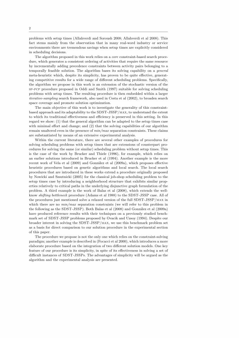
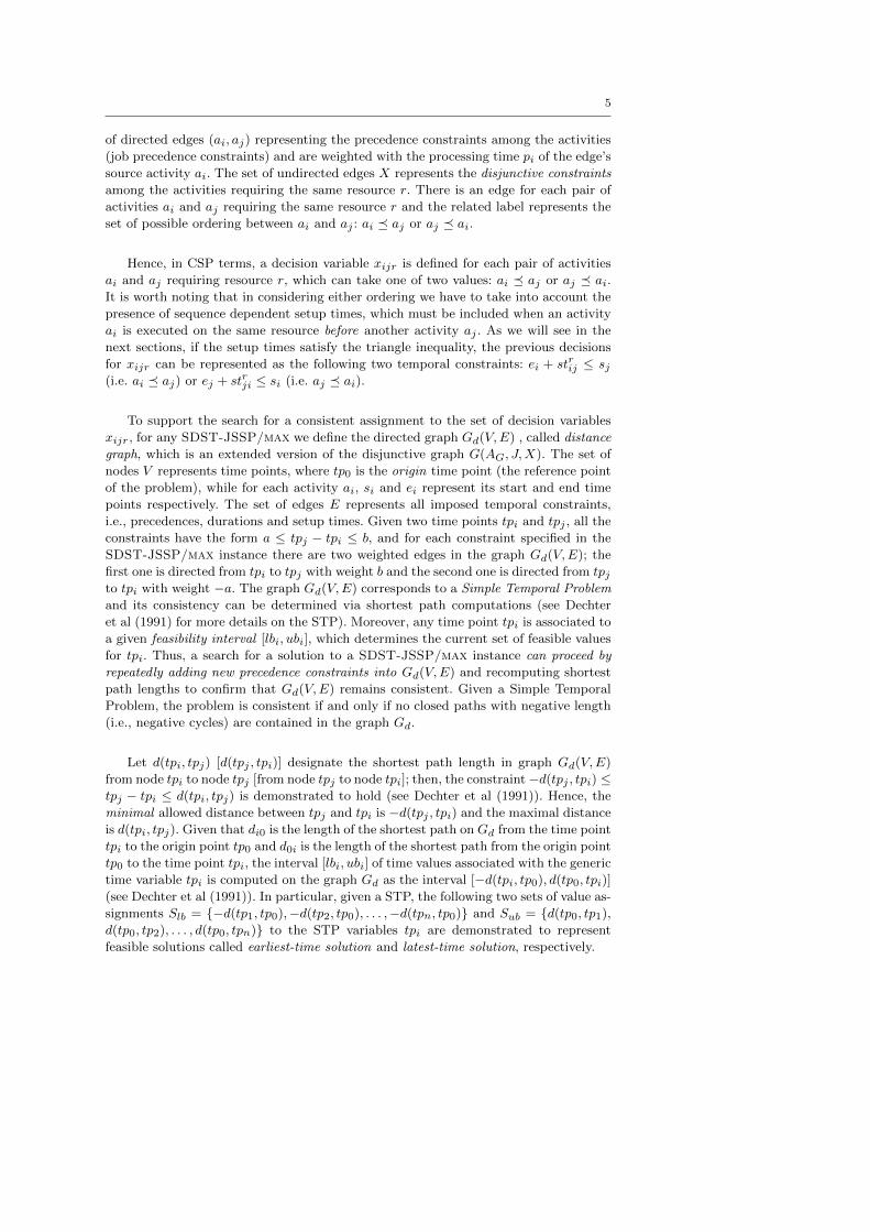
Fig. 2 slack(ei, sj) = d(ei, sj)− strij Vs. co-slack(ei, sj) = −d(sj , ei)− strij

The first way of exploiting shortest path information is by introducing new dom-

inance conditions (which adapt those presented in Oddi and Smith (1997) to the

setup times case), through which problem constraints are propagated and uncondi-

tional decisions for promoting early pruning of alternatives are identified. The con-

cepts of slack(ei, sj) and co-slack(ei, sj) (complementary slack) play a central role in

the definition of such new dominance conditions. Given two activities ai, aj and the

related interval of distances [−d(sj , ei), d(ei, sj)] 1 and [−d(si, ej), d(ej , si)]2 on the

graph Gd, they are defined as follows (see Figure 2):

– slack(ei, sj) = d(ei, sj) − strij is the difference between the maximal distance

d(ei, sj) and the setup time strij . Hence, it provides a measure of the degree of

sequencing flexibility between ai and aj3 taking into account the setup time con-

straint ei + strij ≤ sj . If slack(ei, sj) < 0, then the ordering ai � aj is not feasible.

– co-slack(ei, sj) = −d(sj , ei)− strij is the difference between the minimum possible

distance between ai and aj , −d(si, ej), and the setup time strij ; if co-slack(ei, sj) ≥0 (in Figure 2 a negative co-slack is represented), then there is no need to separate

ai and aj , as the setup time constraint ei + strij ≤ sj is already satisfied.

For any pair of activities ai and aj that are competing for the same resource r, the

new dominance conditions describing the four possible cases of conflict are defined as

1 Between the end-time ei of ai and the start-time sj of aj2 Between the end-time ej of aj and the start-time si of ai3 Intuitively, the higher is the degree of sequencing flexibility, the larger is the set of feasible

assignments to the start-times of ai and aj

7

follows:1. slack(ei, sj) < 0 ∧ slack(ej , si) < 0

2. slack(ei, sj) < 0 ∧ slack(ej , si) ≥ 0 ∧ co-slack(ej , si) < 0

3. slack(ei, sj) ≥ 0 ∧ slack(ej , si) < 0 ∧ co-slack(ei, sj) < 0

4. slack(ei, sj) ≥ 0 ∧ slack(ej , si) ≥ 0

Condition 1 represents an unresolvable conflict. There is no way to order ai and ajtaking into account the setup times strij and strji, without inducing a negative cycle in

the graph Gd(V,E). When Condition 1 is verified the search has reached an inconsistent

state.

Conditions 2, and 3, alternatively, distinguish uniquely resolvable conflicts, i.e.,

there is only one feasible ordering of ai and aj , and the decision of which constraint

to post is thus unconditional. If Condition 2 is verified, only aj � ai leaves Gd(V,E)

consistent. It is worth noting that the presence of the condition co-slack(ej , si) < 0

entails that the minimal distance between the end time ej and the start time si is

shorter than the minimal required setup time strji; hence, we still need to impose the

constraint ej + strji ≤ si. In other words, the co-slack condition avoids the imposition

of unnecessary precedence constraints for trivially solved conflicts. Condition 3 works

similarly, and entails that only the ai � aj ordering is feasible.

Finally, Condition 4 designates a class of resolvable conflicts; in this case, both

orderings of ai and aj remain feasible, and it is therefore necessary to perform a search

decision.

The second way of exploiting shortest path information is by defining variable and

value ordering heuristics for selecting and resolving conflicts in the set characterized

by Condition 4. As stated above, in this context slack(ei, sj) and slack(ej , si) provide

measures of the degree of sequencing flexibility between ai and aj . The variable ordering

heuristic attempts to focus first on the conflict with the least amount of sequencing

flexibility (i.e., the conflict that is closest to previous Condition 1). More precisely, the

conflict (ai, aj) with the overall minimum value of V arEval(ai, aj) = min{bdij , bdji} is

always selected for resolution, where the biased distance terms are defined as follows:4:

bdij =slack(ei,sj)√

S, bdji =

slack(ej ,si)√S

and

S =min{slack(ei, sj), slack(ej , si)}max{slack(ei, sj), slack(ej , si)}

As opposed to variable ordering, the value ordering heuristic attempts to resolve the

selected conflict (ai, aj) simply by choosing the precedence constraint that retains the

highest amount of sequencing flexibility. Specifically, ai � aj is selected if bdij > bdjiand aj � ai is selected otherwise.

4.1 The pcp Algorithm

Figure 3 gives the basic overall pcp solution procedure, which starts from an empty

solution (Step 1) where the graphs Gd is initialized according to Section 3. Also, the

4 The√S bias is introduced to take into account cases where a first conflict with the overall

min{slack(ei, sj), slack(ej , si)} has a very largemax{slack(ei, sj), slack(ej , si)}, and a secondconflict has two shortest path values just slightly larger than this overall minimum. In suchsituations, it is not clear which conflict has the least sequencing flexibility.

8

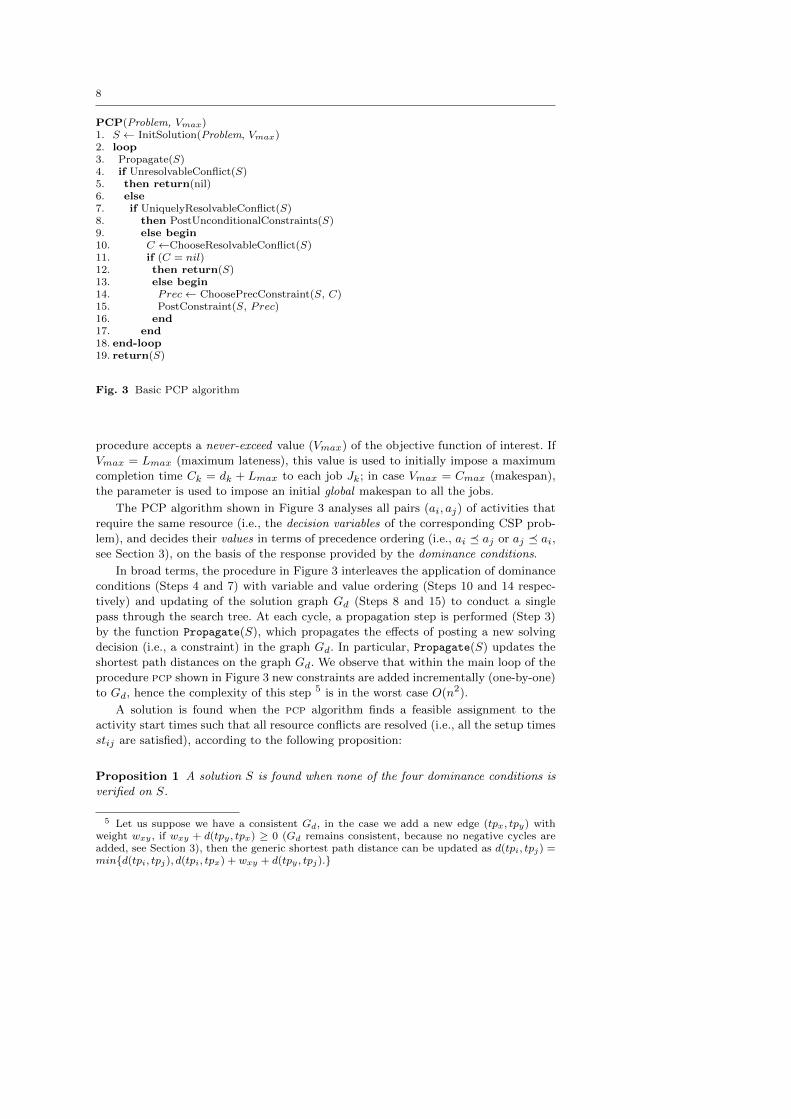
PCP(Problem, Vmax)1. S ← InitSolution(Problem, Vmax)2. loop3. Propagate(S)4. if UnresolvableConflict(S)5. then return(nil)6. else7. if UniquelyResolvableConflict(S)8. then PostUnconditionalConstraints(S)9. else begin10. C ←ChooseResolvableConflict(S)11. if (C = nil)12. then return(S)13. else begin14. Prec← ChoosePrecConstraint(S, C)15. PostConstraint(S, Prec)16. end17. end18. end-loop19. return(S)

Fig. 3 Basic PCP algorithm

procedure accepts a never-exceed value (Vmax) of the objective function of interest. If

Vmax = Lmax (maximum lateness), this value is used to initially impose a maximum

completion time Ck = dk + Lmax to each job Jk; in case Vmax = Cmax (makespan),

the parameter is used to impose an initial global makespan to all the jobs.

The PCP algorithm shown in Figure 3 analyses all pairs (ai, aj) of activities that

require the same resource (i.e., the decision variables of the corresponding CSP prob-

lem), and decides their values in terms of precedence ordering (i.e., ai � aj or aj � ai,see Section 3), on the basis of the response provided by the dominance conditions.

In broad terms, the procedure in Figure 3 interleaves the application of dominance

conditions (Steps 4 and 7) with variable and value ordering (Steps 10 and 14 respec-

tively) and updating of the solution graph Gd (Steps 8 and 15) to conduct a single

pass through the search tree. At each cycle, a propagation step is performed (Step 3)

by the function Propagate(S), which propagates the effects of posting a new solving

decision (i.e., a constraint) in the graph Gd. In particular, Propagate(S) updates the

shortest path distances on the graph Gd. We observe that within the main loop of the

procedure pcp shown in Figure 3 new constraints are added incrementally (one-by-one)

to Gd, hence the complexity of this step 5 is in the worst case O(n2).

A solution is found when the pcp algorithm finds a feasible assignment to the

activity start times such that all resource conflicts are resolved (i.e., all the setup times

stij are satisfied), according to the following proposition:

Proposition 1 A solution S is found when none of the four dominance conditions is

verified on S.

5 Let us suppose we have a consistent Gd, in the case we add a new edge (tpx, tpy) withweight wxy , if wxy + d(tpy , tpx) ≥ 0 (Gd remains consistent, because no negative cycles areadded, see Section 3), then the generic shortest path distance can be updated as d(tpi, tpj) =min{d(tpi, tpj), d(tpi, tpx) + wxy + d(tpy , tpj).}

9

The previous assertion can be demonstrated by contradiction. Let us suppose that

the pcp procedure exits with success (none of the four dominance conditions is verified

on S) and that at least two sequential activities ai and aj , requiring the same resource

r do not satisfy the setup constraints ei + strij ≤ sj or ej + strji ≤ si. Since the

triangle inequality holds for the input problem, it is guaranteed that the length of the

direct setup transition ai � aj between two generic activities ai and aj is the shortest

possible (i.e., no indirect transition ai ; ak ; aj having a shorter overall length

can exist). This fact is relevant for the pcp approach, because the solving algorithm

proceeds by checking/imposing either the constraint ei + strij ≤ sj or the constraint

ej + strji ≤ si for each pair of activities. Hence, when none of the four dominance

conditions is verified, each subset of activities Ar requiring the same resource r is

totally ordered over time. Clearly, for each pair (ai, aj), such that ai, aj ∈ Ar, either

co-slack(ei, sj) ≥ 0 or co-slack(ej , si) ≥ 0; hence, all pairs of activities (ai, aj) requiring

the same resource r satisfy the setup constraints ei+strij ≤ sj or ej +strji ≤ si. In fact,

by definition co-slack(ei, sj) ≥ 0 implies −d(sj , ei) ≥ strij and together the condition

sj − ei ≥ −d(sj , ei) (which holds because Gd is consistent, see Section 3), we have

ei + strij ≤ sj (a similar proof is given for co–slack(ej , si) ≥ 0).

To wrap up, when none of the four dominance conditions is verified, and the pcp

procedure exits with success, the Gd graph represents a consistent Simple Temporal

Problem and, as described in Section 3, one possible solution of the problem is the

so-called earliest-time solution, such that Sest = {Si = −d(tpi, tp0) : i = 1 . . . n}.

5 An Iterative Sampling Procedure

The pcp resolution procedure, as defined above, is a deterministic (partial) solution

procedure with no recourse in the event that an unresolved conflict is encountered.

To provide a capability for expanding the search in such cases without incurring the

combinatorial overhead of a conventional backtracking search, in the following two

subsections we define:

1. a random counterpart of our conflict selection heuristic (in the style of Oddi and

Smith (1997)), providing stochastic variable and value ordering heuristics;

2. an iterative sampling search framework for optimization embedding the stochastic

procedure.

This choice is motivated by the observation that in many cases systematic back-

tracking search can explore large sub-trees without finding a solution (this behavior

is also known as thrashing in the Constraint Proramming area, see Cambazard et al

(2008)). On the other hand, if we compare the whole search tree created by a system-

atic search algorithm with the non systematic tree explored by repeatedly restarting

a randomized search algorithm, we see that the randomized procedure is able to reach

“different and distant” leaves in the search tree. The latter property could be an ad-

vantage when problem solutions are uniformly distributed within the set of search tree

leaves interleaved with large sub-trees which do not contain any problem solution.

5.1 Stochastic Variable and Value Ordering

The stochastic versions of pcp’s variable and value ordering heuristics follows from the

simple intuition that it generally makes more sense to follow a heuristic’s advice when

10

the heuristic clearly distinguishes one alternative as superior, while it makes less sense

to follow its advice when several choices are judged to be equally good.

Let us consider first the case of variable ordering. As previously discussed, pcp’s

variable ordering heuristic selects the conflict (ai, aj) with the overall minimum value of

V arEval(ai, aj) = min{bdij , bdji}. If V arEval(ai, aj) is << than V arEval(ak, al) for

all other pending conflicts (ak, al), then the conflict (ai, aj) is clearly recognized as the

one to be selected. However, if more V arEval(ak, al) values are instead quite “close”

to V arEval(ai, aj), then the choice to be preferred is not so clear and the selection

of any of these conflicts may be reasonable. We formalize this notion by defining an

acceptance band β with respect to the set of pending resolvable conflicts and expanding

the pcp ChooseResolvable-Conflict routine in the following three steps:

1. Calculate the overall minimum value

ω = min{V arEval(ai, aj)}

2. Determine the subset SC of resolvable conflicts

SC = {(ai, aj) : ω ≤ V arEval((ai, aj)) ≤ ω(1 + β)}

3. Randomly select a conflict (ai, aj) in the set SC.

Thus, β defines a range around the minimum (i.e., best) heuristic evaluation within

which all differences in value are assumed to be insignificant and non-informative. The

smaller the value of β, the higher the assumed discriminatory power of the heuristic.

A similar approach can be chosen for value ordering decisions. Let pc(ai, aj) be the

deterministic value ordering heuristic used by pcp. As previously noted, pc(ai, aj) =

ai � aj when bdij > bdji, and aj � ai otherwise. Recalling the definition of the biased

distance bd, in cases where S =min{slack(ei,sj),slack(ej ,si)}max{slack(ei,sj),slack(ej ,si)} is ≈ 1, and hence bdij and

bdji are almost equal, pc(ai, aj) does not yield a clear guidance (both choices appear

equally good). Therefore, we define the following randomized version of ChoosePrec-

Constraint:

rpc(ai, aj) =

{pc(ai, aj) : U [0, 1] + α < S

pc(ai, aj) : otherwise

where α represents a threshold parameter, U [0, 1] represents a random value in the

interval [0, 1] with uniform distribution function, and pc(ai, aj) is the complement of

the choice advocated by pc(ai, aj). Under this random selection method, it is simple to

demonstrate that the probability of deviating from the choice of PCP’s original value

ordering heuristic pc is (S − α) when S ≥ α and 0 otherwise. If α is set to 0.5, then

each ordering choice can be seen to be equally likely in the case where S = 1 (i.e., the

case where the heuristic gives the least information).

5.2 The Optimization Algorithm

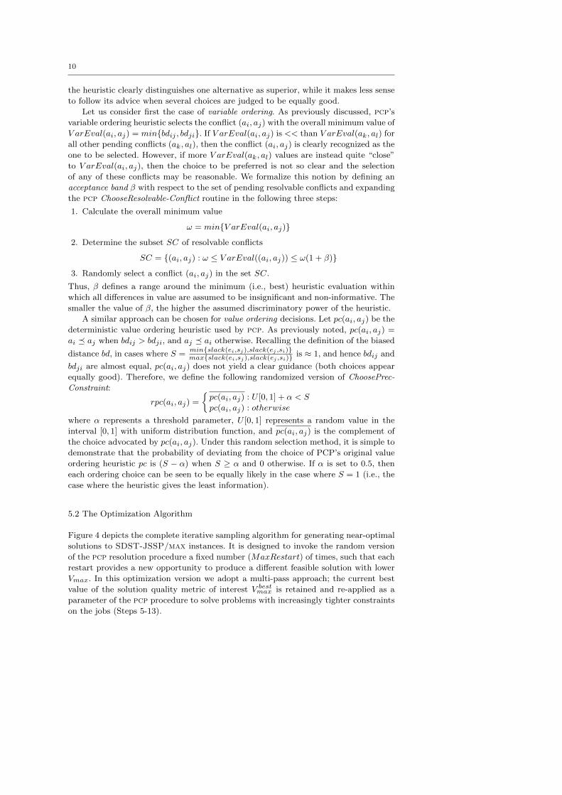
Figure 4 depicts the complete iterative sampling algorithm for generating near-optimal

solutions to SDST-JSSP/max instances. It is designed to invoke the random version

of the pcp resolution procedure a fixed number (MaxRestart) of times, such that each

restart provides a new opportunity to produce a different feasible solution with lower

Vmax. In this optimization version we adopt a multi-pass approach; the current best

value of the solution quality metric of interest V bestmax is retained and re-applied as a

parameter of the pcp procedure to solve problems with increasingly tighter constraints

on the jobs (Steps 5-13).

11

ISP(Problem, V(0)max, MaxRestart)

1. S ← EmptySolution(Problem, V(0)max)

2. Sbest ← S

3. V bestmax ← V

(0)max

4. count← 05. while (count ≤MaxRestart) do begin6. S ← PCP(Problem, V best

max)7. if (Vmax(S) < V best

max)8. then begin9. Sbest ← S10. V best

max ← Vmax(S)11. end12. count← count+ 113. end-while14. return(Sbest)

Fig. 4 Iterative sampling algorithm

6 Experimental Analysis

In this section we propose a set of empirical evaluations of the isp algorithm shown in

Figure 4. We remark that in the tested version of the isp algorithm we use a uniform

distribution probability to implement both random variable and value ordering heuris-

tics 6. The isp algorithm has been implemented in CMU Common Lisp Ver. 20a and

run on a AMD Phenom II X4 Quad 3.5 Ghz under Linux Ubuntu 10.04.1.

We observe that, to the best of our knowledge, there are no standard benchmarks

available for the full version of the SDST-JSSP/max problems (i.e., SDST-JSSP

problems that additionally include min/max separation constraints). For this reason,

we first consider some classical benchmarks of SDST-JSSP described in literature and

available on the Internet. Such benchmarks represent a relaxed version of the SDST-

JSSP/max problem introduced in the first part of the paper. Later, we will define a

new benchmark set for the full SDST-JSSP/max, and for this new benchmark a first

set of experimental results will be provided.

Since we are proposing a heuristic algorithm that incorporates two basic param-

eters - α and β, we face the problem of tuning our heuristic approach. We use the

racing procedure F-Race proposed in Birattari et al (2002) to find a configuration of

the algorithm that performs as well as possible on a given instance class of a combina-

torial optimization problem. This method takes inspiration from the Machine Learning

(ML) literature for model selection through cross-validation. The F-Race procedure em-

pirically evaluates a set of candidate configurations by discarding bad ones as soon as

statistically sufficient evidence has been gathered against them. The advantage in using

such approach for tuning parameters is twofold. First, F-Race is able to quickly reduce

the number of candidates, and narrow focus to the most promising ones. Second, this

methodology allows comparison of results on different instances independently of the

6 In particular, for variable ordering we select at random one element in the set SC ={(ai, aj) : ω ≤ V arEval((ai, aj)) ≤ ω(1 + β)} with uniform distribution probability (see Sec-tion 5.1). About random value ordering, we exchange the precedence constraint determined viathe deterministic value ordering heuristic on the basis of the test U [0, 1]+α < S, where U [0, 1]represents a random value in the interval [0, 1] with uniform distribution (see Section 5.1).

12

inherent difference in the cost functions. More specifically in our analysis we perform

a F-Race selection based on Friedman analysis of variance by ranks as implemented in

the Race package (Birattari (2010)) available for the R statistical software - R Devel-

opment Core Team (2010).

6.1 Empirical Analysis on Existing Benchmarks

As indicated above, we start in this section by analyzing the performance of the isp

algorithm on selected SDST-JSSP benchmark sets that can be found in literature.

This allows us to test our algorithm against the best results currently available, in

order to get an idea of its effectiveness when compared with different existing solving

approaches. In this way, we intend to provide an added value to the subsequent analysis

of the algorithm’s performance on problem instances of the full SDST-JSSP/max (see

Section 6.3), for which, we have no competitors as yet.

Our analysis on SDST-JSSP benchmarks proceeds as follows. In Section 6.1.1 the

isp algorithm is employed to solve the SDST-JSSP benchmark proposed in Ovacik

and Uzsoy (1994); Demirkol et al (1998). In this case, the objective is minimization

of maximum lateness (Lmax). We perform a series of both explorative and selective

experimental runs that vary the algorithm’s randomization parameters α and β. Sec-

tion 6.1.2 then is dedicated to analyzing the performance of our algorithm on a second

SDST-JSSP benchmark originally proposed in Brucker and Thiele (1996). In this case,

the objective is to minimize the makespan (Cmax). We again perform a series of both

explorative and selective experimental runs using different α and β randomization pa-

rameters.

6.1.1 Lmax minimization

The first benchmarks we consider are proposed in Demirkol et al (1998); Ovacik and

Uzsoy (1994), and are available at http://pst.istc.cnr.it/~angelo/OUdata/. In or-

der to comprehensively interpret the experimental results, it is necessary to provide a

brief description of how these benchmarks were originally produced. In all benchmark

instances, the setup times strij and the processing times pi of every activity ai are val-

ues randomly computed in the interval [1, 200]. The job due dates di are assumed to be

uniformly distributed over an interval I characterized by the following two parameters:

(1) the mean value µ = (1 − τ)E[Cmax], where τ denotes the percentage of jobs that

are expected to be tardy and E[Cmax] is the expected makespan7, and (2) the R value,

which determines the range of I, whose bounds are defined by: [µ(1−R/2), µ(1+R/2)].

All benchmark instances are calculated using the τ values of 0.3 and 0.6, corresponding

to loose and tight due dates respectively, and the R values of 0.5, 1.5 and 2.5, respec-

tively modeling different due date variation levels. The particular combination of the τ

and R values allows us to categorize all instances into six different benchmarks, namely:

i305, i315, i325, i605, i615, i625. Each benchmark contains 160 randomly generated

problem instances, divided in subclasses based on the numbers of machines and jobs

involved; more precisely, all instances are synthesized by choosing 10 and 20 jobs on 5,

10, 15 and 20 machines, yielding a total of 8 subclasses for each benchmark.

7 Calculated by estimating the total setup and processing time required by all jobs at allmachines and dividing the result by the number of available machines.

13

One implication of this procedure for generating problem instances is that this

benchmark does not satisfy the triangle inequality, as all setup times and activity

durations are computed in the interval [1, 200] at random. This fact has important

consequences on our Iterative Sampling Algorithm (see Figure 4), as it may cause the

algorithm to disregard a number of valid solutions due to constraint overcommitment.

As indicated earlier, the triangle inequality condition guarantees that the length of the

direct setup transition ai � aj between two generic activities ai and aj is the shortest

possible and it is not possible to find an indirect transition (a sequence of activities

ai ; ak ; aj) which has a shorter overall length. The pcp approach relies on this

property, as the solving algorithm proceeds by checking/imposing either the constraint

ei + strij ≤ sj or the constraint ej + strji ≤ si for any given pair of activities competing

for the same resource. Hence, if the triangular inequality does not hold, the procedure

might post over-committing constraints during the solving process, which (a) increases

the probability of finding sub-optimal solutions and (b) introduces the possibility that

some solutions may be disregarded.

To illustrate the potential problem due to over-commitment, consider three activi-

ties a1, a2 and a3 requiring the same resource, with processing times p1 = p2 = p3 = 1

and setup times st12 = st21 = 15, st13 = st31 = 3 and st23 = st32 = 3. Suppose

also that the overall scheduling horizon is limited to 10. Under these conditions, the

triangle inequality for the setup times is clearly not satisfied, and our pcp procedure

is prone to failure. Specifically, the first dominance condition is verified for the activ-

ity pair 〈a1, a2〉 (detecting an unresolvable conflict), despite the fact that the solution

a1 � a3 � a2 does exist. In fact, the algorithm will try to impose one of the two

setup constraints st12 = st21 = 15, but both are in conflict with the horizon constraint

(15 > 10).

This characteristic of the benchmark definitely puts the isp algorithm at a dis-

advantage. However, a straightforward probabilistic computation allows us to easily

determine the probability that the triangular inequality will not be satisfied by a given

triple of activities; and this value is as low as 4.04%. This suggests that use of the tri-

angular inequality assumption can still be considered as viable, as it is in fact satisfied

in the vast majority of the cases. Indeed, this explains the globally strong performance

of the algorithm on these instances (see below).

Despite the low probability of the triangular inequality being violated, we opted

to apply a post-processing step similar to the Chaining of Policella et al (2007) to the

solution S generated by the pcp algorithm in Figure 3, to eliminate any constraint

overcommitments that may have been introduced, and thus improve the solution qual-

ity by left-shifting some of the jobs. This post-processing phase is accomplished in two

steps. First, all previously posted ordering constraints are removed from the solution S.

Second, for each resource and for each activity ai (in increasing order of the determined

sequence in which activities use the resource), the unique successor aj is considered,

and the precedence constraints ei + strij ≤ sj is posted. This last step is iterated un-

til all activities are linked by the correct sequence dependent setup times provided in

the problem definition. Then, a new earliest start time solution is recomputed on the

basis of the newly imposed constraints via shortest path computation on the graph

Gd representation. We observe that the set of imposed constraints surely represents a

solution of the problem because this new set of constraints is less restrictive than the

previous one.

In what follows we perform a two-step analysis. An initial, broad analysis of the

independent effects of random value ordering and random variable ordering configu-

14

rations is first carried out on all six benchmark sets (i305, i315, i325, i605, i615, and

i625) with different computational time limits. Next, a second, more fine-grained anal-

ysis of the effects of the α (random value ordering) and β (random variable ordering)

parameters is performed using the above cited F-Race technique on the two benchmark

sets for which the ISP algorithm achieved its worst and best performance respectively

in the initial analysis step.

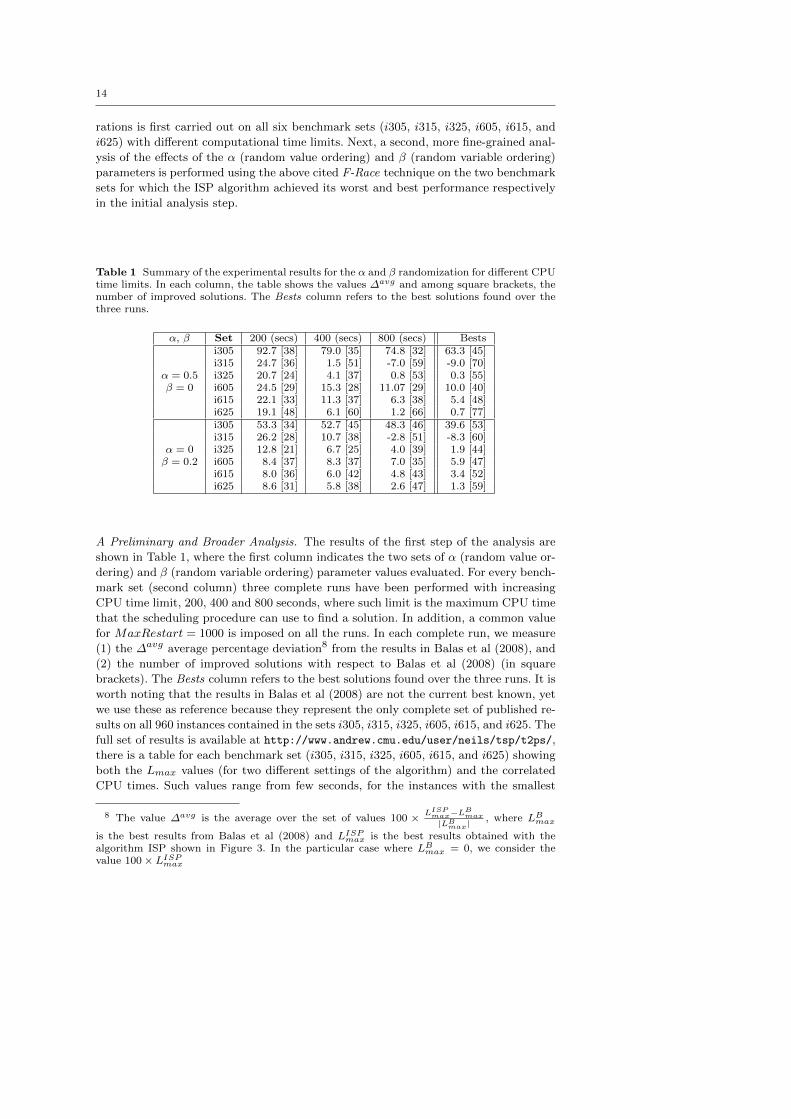
Table 1 Summary of the experimental results for the α and β randomization for different CPUtime limits. In each column, the table shows the values ∆avg and among square brackets, thenumber of improved solutions. The Bests column refers to the best solutions found over thethree runs.

α, β Set 200 (secs) 400 (secs) 800 (secs) Bestsi305 92.7 [38] 79.0 [35] 74.8 [32] 63.3 [45]i315 24.7 [36] 1.5 [51] -7.0 [59] -9.0 [70]

α = 0.5 i325 20.7 [24] 4.1 [37] 0.8 [53] 0.3 [55]β = 0 i605 24.5 [29] 15.3 [28] 11.07 [29] 10.0 [40]

i615 22.1 [33] 11.3 [37] 6.3 [38] 5.4 [48]i625 19.1 [48] 6.1 [60] 1.2 [66] 0.7 [77]i305 53.3 [34] 52.7 [45] 48.3 [46] 39.6 [53]i315 26.2 [28] 10.7 [38] -2.8 [51] -8.3 [60]

α = 0 i325 12.8 [21] 6.7 [25] 4.0 [39] 1.9 [44]β = 0.2 i605 8.4 [37] 8.3 [37] 7.0 [35] 5.9 [47]

i615 8.0 [36] 6.0 [42] 4.8 [43] 3.4 [52]i625 8.6 [31] 5.8 [38] 2.6 [47] 1.3 [59]

A Preliminary and Broader Analysis. The results of the first step of the analysis are

shown in Table 1, where the first column indicates the two sets of α (random value or-

dering) and β (random variable ordering) parameter values evaluated. For every bench-

mark set (second column) three complete runs have been performed with increasing

CPU time limit, 200, 400 and 800 seconds, where such limit is the maximum CPU time

that the scheduling procedure can use to find a solution. In addition, a common value

for MaxRestart = 1000 is imposed on all the runs. In each complete run, we measure

(1) the ∆avg average percentage deviation8 from the results in Balas et al (2008), and

(2) the number of improved solutions with respect to Balas et al (2008) (in square

brackets). The Bests column refers to the best solutions found over the three runs. It is

worth noting that the results in Balas et al (2008) are not the current best known, yet

we use these as reference because they represent the only complete set of published re-

sults on all 960 instances contained in the sets i305, i315, i325, i605, i615, and i625. The

full set of results is available at http://www.andrew.cmu.edu/user/neils/tsp/t2ps/,

there is a table for each benchmark set (i305, i315, i325, i605, i615, and i625) showing

both the Lmax values (for two different settings of the algorithm) and the correlated

CPU times. Such values range from few seconds, for the instances with the smallest

8 The value ∆avg is the average over the set of values 100 × LISPmax−LB

max|LB

max|, where LB

max

is the best results from Balas et al (2008) and LISPmax is the best results obtained with the

algorithm ISP shown in Figure 3. In the particular case where LBmax = 0, we consider the

value 100× LISPmax

15

size, to about one hundred seconds for the largest ones. More recent results represent-

ing the current best are published in Gonzalez et al (2009a) for the i305 set only. The

authors of Gonzalez et al (2009a) have also kindly provided us with (as yet unreleased)

results extended to all the benchmark sets [Gonzalez et al (2009b)]. These results are

summarized in the GV V 09 column of Table 2.

Returning to Table 1, the top half indicates the results obtained when randomiza-

tion is restricted to value ordering decisions and variable ordering decisions are made

deterministically (i.e., α = 0.5 and β = 0). Even though this analysis represents an

initial baseline configuration, the results are nonetheless interesting as this configura-

tion of the algorithm finds a considerable number of improved solutions in all cases.

The best performance seems to involve the benchmarks associated with higher values

of the R parameter; as the table shows, the outcomes are much more convincing when

R is greater or equal than 1.5, i.e., when the level of the due date variation is higher.

One possible explanation for this behavior is the following. As the value of R increases,

the due dates of jobs are randomly chosen from a wider set of uniformly distributed

values; this implies that, among all generated due dates, there will be a subset that are

particularly tight (i.e., the earliest deadlines). Given the design of the pcp scheduling

procedure (see Figure 3), solutions are found by imposing the deadlines of the most

“critical” jobs (i.e., the jobs characterized by the earliest deadlines)9. In other words,

the procedure naturally proceeds by first accommodating the most critical jobs, by

imposing “hard” deadline constraints, and then secondly addressing the “easier” task

of accommodating the remaining jobs. On the contrary, when the R values are lower,

all generated due dates tend to be critical, as all their values are comparable and hence

indistinguishable. This circumstance may represent an obstacle to good performance

in the current version of the procedure, in that low-lateness scheduling for all jobs by

means of imposing hard constraints cannot be always guaranteed. As we are running a

random solving procedure, we finally observe that the overall results can be improved

by considering the best solutions over the set of the performed runs. In Table 1, the

column labelled Bests shows a significant performance improvement in comparison to

the three individual runs.

The bottom half of Table 1 shows the results for random variable ordering (i.e.,

α = 0 and β = 0.2). As in the previous case, the best performance seems to involve the

benchmarks associated with higher values of R (1.5 and 2.5). However, there are also

some differences. The most evident is that the results obtained with random variable

ordering are in some sense complementary with the results for random value ordering.

In fact, Table 1 shows that the best results for the i305 and i605 benchmarks (R = 0.5)

are obtained in the random variable ordering case (lower half of the table), while the

best results for the i315, i325, i615 and i625 benchmarks (R = 1.5 and R = 2.5), are

obtained in the random value ordering case (upper half of the table).

In Table 2 we summarize the best results obtained using both the random value

randomization and the random variable randomization procedures (the two columns

labeled Bests(α) and Bests(β)), as well as the best overall performance (the column

labeled BESTS). Observing the best overall performance, we see that our algorithm

yields significant improvement in terms of number of improved solutions; in fact, we are

able to find better solutions for 396 of the 960 total instances in the overall benchmark.

Moreover, we also observe very good performance in average percentage deviation

9 Due to the “most constrained first” approach used in the pcp procedure on conflict selec-tion, line 9.

16

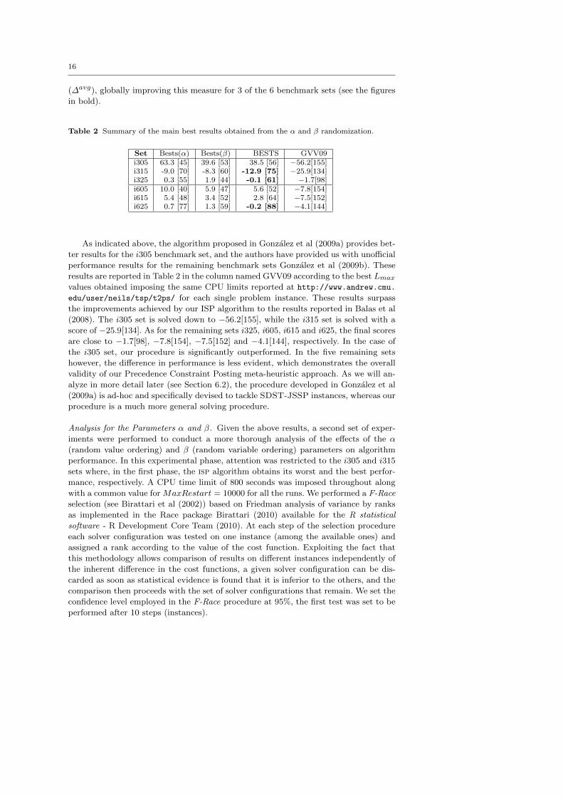
(∆avg), globally improving this measure for 3 of the 6 benchmark sets (see the figures

in bold).

Table 2 Summary of the main best results obtained from the α and β randomization.

Set Bests(α) Bests(β) BESTS GVV09i305 63.3 [45] 39.6 [53] 38.5 [56] −56.2[155]i315 -9.0 [70] -8.3 [60] -12.9 [75] −25.9[134]i325 0.3 [55] 1.9 [44] -0.1 [61] −1.7[98]i605 10.0 [40] 5.9 [47] 5.6 [52] −7.8[154]i615 5.4 [48] 3.4 [52] 2.8 [64] −7.5[152]i625 0.7 [77] 1.3 [59] -0.2 [88] −4.1[144]

As indicated above, the algorithm proposed in Gonzalez et al (2009a) provides bet-

ter results for the i305 benchmark set, and the authors have provided us with unofficial

performance results for the remaining benchmark sets Gonzalez et al (2009b). These

results are reported in Table 2 in the column named GVV09 according to the best Lmax

values obtained imposing the same CPU limits reported at http://www.andrew.cmu.

edu/user/neils/tsp/t2ps/ for each single problem instance. These results surpass

the improvements achieved by our ISP algorithm to the results reported in Balas et al

(2008). The i305 set is solved down to −56.2[155], while the i315 set is solved with a

score of −25.9[134]. As for the remaining sets i325, i605, i615 and i625, the final scores

are close to −1.7[98], −7.8[154], −7.5[152] and −4.1[144], respectively. In the case of

the i305 set, our procedure is significantly outperformed. In the five remaining sets

however, the difference in performance is less evident, which demonstrates the overall

validity of our Precedence Constraint Posting meta-heuristic approach. As we will an-

alyze in more detail later (see Section 6.2), the procedure developed in Gonzalez et al

(2009a) is ad-hoc and specifically devised to tackle SDST-JSSP instances, whereas our

procedure is a much more general solving procedure.

Analysis for the Parameters α and β. Given the above results, a second set of exper-

iments were performed to conduct a more thorough analysis of the effects of the α

(random value ordering) and β (random variable ordering) parameters on algorithm

performance. In this experimental phase, attention was restricted to the i305 and i315

sets where, in the first phase, the isp algorithm obtains its worst and the best perfor-

mance, respectively. A CPU time limit of 800 seconds was imposed throughout along

with a common value for MaxRestart = 10000 for all the runs. We performed a F-Race

selection (see Birattari et al (2002)) based on Friedman analysis of variance by ranks

as implemented in the Race package Birattari (2010) available for the R statistical

software - R Development Core Team (2010). At each step of the selection procedure

each solver configuration was tested on one instance (among the available ones) and

assigned a rank according to the value of the cost function. Exploiting the fact that

this methodology allows comparison of results on different instances independently of

the inherent difference in the cost functions, a given solver configuration can be dis-

carded as soon as statistical evidence is found that it is inferior to the others, and the

comparison then proceeds with the set of solver configurations that remain. We set the

confidence level employed in the F-Race procedure at 95%, the first test was set to be

performed after 10 steps (instances).

17

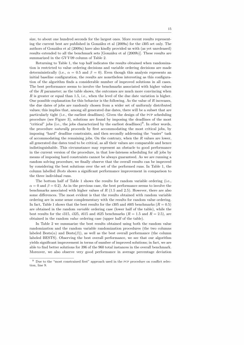
This phase of the analysis was carried out in two steps. In the first step, for each

of the two sets i305 and i315 we selected 20 instances (in particular the instances

21-40) and performed a F-Race selection of the effects on performance of various α

and β parameter configurations. In the second step, we ran a selective analysis for the

values α and β that yielded the best results in the first step, and compared the results

obtained to the best known results available in the literature.

alpha−1.0−−beta−0.05alpha−0.8−−beta−0.0



alpha−0.9−−beta−0.1alpha−0.75−−beta−0.0alpha−0.85−−beta−0.1alpha−1.0−−beta−0.01alpha−1.0−−beta−0.01alpha−0.85−−beta−0.2

alpha−0.95−−beta−0.15alpha−0.85−−beta−0.15alpha−0.75−−beta−0.05alpha−0.85−−beta−0.0






alpha−0.9−−beta−0.0alpha−0.85−−beta−0.25alpha−0.8−−beta−0.25


0 1 2 3 4 5 6 7 8 9 10 12 14 16 18 20

Iterated Sampling Procedure −− screening−i305 (20 Instances)

Stage

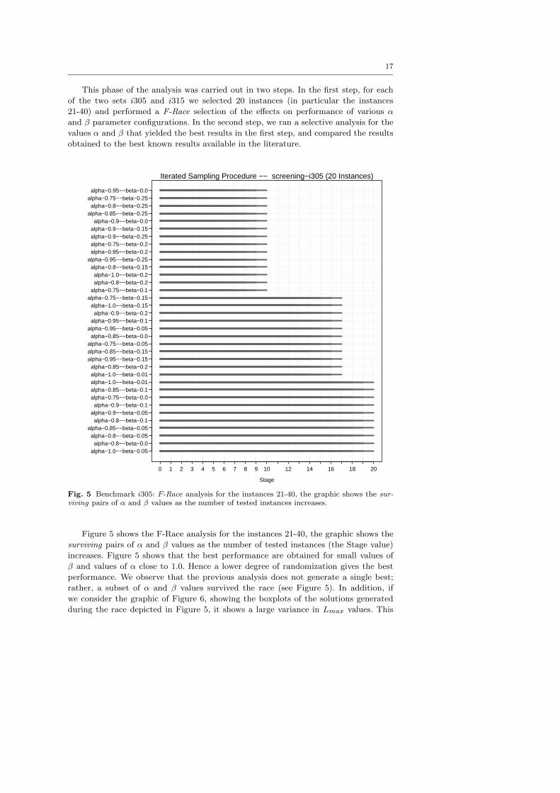
Fig. 5 Benchmark i305: F-Race analysis for the instances 21-40, the graphic shows the sur-viving pairs of α and β values as the number of tested instances increases.

Figure 5 shows the F-Race analysis for the instances 21-40, the graphic shows the

surviving pairs of α and β values as the number of tested instances (the Stage value)

increases. Figure 5 shows that the best performance are obtained for small values of

β and values of α close to 1.0. Hence a lower degree of randomization gives the best

performance. We observe that the previous analysis does not generate a single best;

rather, a subset of α and β values survived the race (see Figure 5). In addition, if

we consider the graphic of Figure 6, showing the boxplots of the solutions generated

during the race depicted in Figure 5, it shows a large variance in Lmax values. This

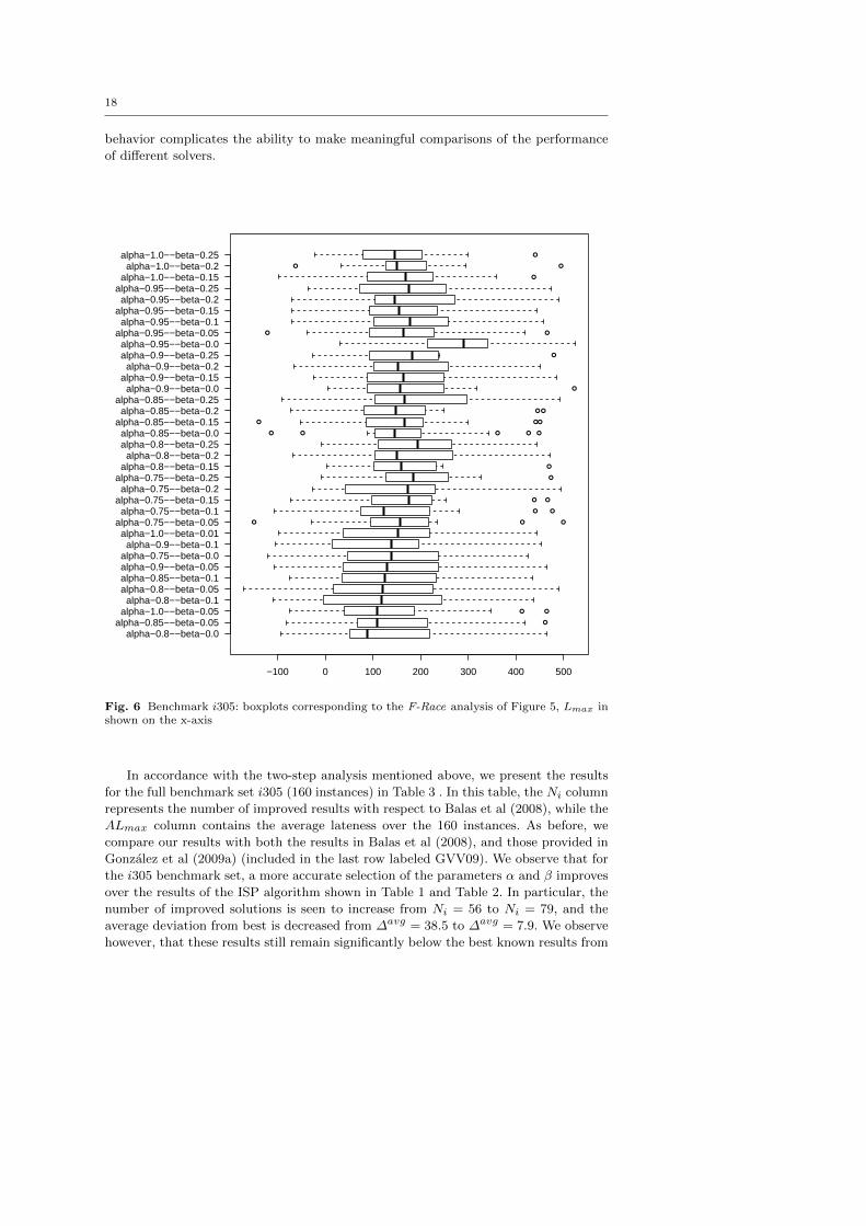
18

behavior complicates the ability to make meaningful comparisons of the performance

of different solvers.

●

●●

●● ●

●●

●●

●

●

●● ●● ●

●● ●

●●

●

●

●●

●

●●

●



alpha−0.8−−beta−0.05alpha−0.85−−beta−0.1alpha−0.9−−beta−0.05alpha−0.75−−beta−0.0





alpha−0.8−−beta−0.2alpha−0.8−−beta−0.25alpha−0.85−−beta−0.0









−100 0 100 200 300 400 500

Fig. 6 Benchmark i305: boxplots corresponding to the F-Race analysis of Figure 5, Lmax inshown on the x-axis

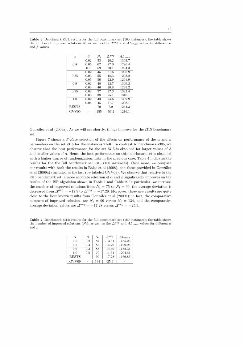
In accordance with the two-step analysis mentioned above, we present the results

for the full benchmark set i305 (160 instances) in Table 3 . In this table, the Ni column

represents the number of improved results with respect to Balas et al (2008), while the

ALmax column contains the average lateness over the 160 instances. As before, we

compare our results with both the results in Balas et al (2008), and those provided in

Gonzalez et al (2009a) (included in the last row labeled GVV09). We observe that for

the i305 benchmark set, a more accurate selection of the parameters α and β improves

over the results of the ISP algorithm shown in Table 1 and Table 2. In particular, the

number of improved solutions is seen to increase from Ni = 56 to Ni = 79, and the

average deviation from best is decreased from ∆avg = 38.5 to ∆avg = 7.9. We observe

however, that these results still remain significantly below the best known results from

19

Table 3 Benchmark i305: results for the full benchmark set (160 instances); the table showsthe number of improved solutions Ni as well as the ∆avg and ALmax values for different αand β values.

α β Ni ∆avg ALmax

0.02 53 20.2 1303.70.8 0.05 62 27.0 1296.4

0.1 59 30.1 1294.30.02 45 21.6 1296.9

0.85 0.03 55 18.3 1293.20.05 56 22.9 1291.9

0.9 0.02 40 22.7 1309.20.03 46 20.8 1299.2

0.95 0.02 27 27.3 1321.40.03 38 25.1 1310.1

1.0 0.02 43 24.6 1309.90.05 45 27.7 1298.1

BESTS - 79 7.9 1244.3

GVV09 - 155 -56.2 1216.1

Gonzalez et al (2009a). As we will see shortly, things improve for the i315 benchmark

set.

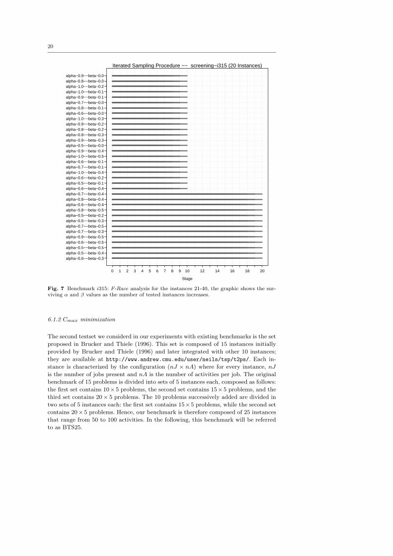
Figure 7 shows a F-Race selection of the effects on performance of the α and β

parameters on the set i315 for the instances 21-40. In contrast to benchmark i305, we

observe that the best performance for the set i315 is obtained for larger values of β

and smaller values of α. Hence the best performance on this benchmark set is obtained

with a higher degree of randomization. Like in the previous case, Table 4 indicates the

results for the the full benchmark set i315 (160 instances). Once more, we compare

our results with both the results in Balas et al (2008), and those provided in Gonzalez

et al (2009a) (included in the last row labeled GVV09). We observe that relative to the

i315 benchmark set, a more accurate selection of α and β significantly improves on the

results of the ISP algorithm shown in Table 1 and Table 2. In particular, we increase

the number of improved solutions from Ni = 75 to Ni = 99, the average deviation is

decreased from ∆avg = −12.9 to ∆avg = −17.28. Moreover, these new results are quite

close to the best known results from Gonzalez et al (2009a); in fact, the comparative

numbers of improved solutions are Ni = 99 versus Ni = 134, and the comparative

average deviation values are ∆avg = −17.28 versus ∆avg = −25.9.

Table 4 Benchmark i315: results for the full benchmark set (160 instances); the table showsthe number of improved solutions (Ni), as well as the ∆avg and ALmax values for different αand β.

α β Ni ∆avg ALmax

0.5 0.2 87 -13.61 1185.260.5 0.4 83 -14.20 1199.960.6 0.3 88 -14.50 1182.341.0 0.5 70 -11.34 1204.51

BESTS - 99 -17.28 1169.86

GVV09 - 134 -25.9 -

20

alpha−0.6−−beta−0.3alpha−0.5−−beta−0.4alpha−0.5−−beta−0.5alpha−0.6−−beta−0.5alpha−0.9−−beta−0.5alpha−0.7−−beta−0.3alpha−0.7−−beta−0.5alpha−0.5−−beta−0.3alpha−0.5−−beta−0.2alpha−0.8−−beta−0.5alpha−0.6−−beta−0.4alpha−0.8−−beta−0.4alpha−0.7−−beta−0.4alpha−0.6−−beta−0.4alpha−0.5−−beta−0.1alpha−0.6−−beta−0.2alpha−1.0−−beta−0.4alpha−0.7−−beta−0.1alpha−0.6−−beta−0.1alpha−1.0−−beta−0.5alpha−0.9−−beta−0.4alpha−0.5−−beta−0.0alpha−0.9−−beta−0.3alpha−0.8−−beta−0.3alpha−0.8−−beta−0.2alpha−0.9−−beta−0.2alpha−1.0−−beta−0.3alpha−0.6−−beta−0.0alpha−0.8−−beta−0.1alpha−0.7−−beta−0.0alpha−0.9−−beta−0.1alpha−1.0−−beta−0.1alpha−1.0−−beta−0.2alpha−0.8−−beta−0.0alpha−0.9−−beta−0.0

0 1 2 3 4 5 6 7 8 9 10 12 14 16 18 20

Iterated Sampling Procedure −− screening−i315 (20 Instances)

Stage

Fig. 7 Benchmark i315: F-Race analysis for the instances 21-40, the graphic shows the sur-viving α and β values as the number of tested instances increases.

6.1.2 Cmax minimization

The second testset we considerd in our experiments with existing benchmarks is the set

proposed in Brucker and Thiele (1996). This set is composed of 15 instances initially

provided by Brucker and Thiele (1996) and later integrated with other 10 instances;

they are available at http://www.andrew.cmu.edu/user/neils/tsp/t2ps/. Each in-

stance is characterized by the configuration (nJ × nA) where for every instance, nJ

is the number of jobs present and nA is the number of activities per job. The original

benchmark of 15 problems is divided into sets of 5 instances each, composed as follows:

the first set contains 10×5 problems, the second set contains 15×5 problems, and the

third set contains 20× 5 problems. The 10 problems successively added are divided in

two sets of 5 instances each: the first set contains 15×5 problems, while the second set

contains 20× 5 problems. Hence, our benchmark is therefore composed of 25 instances

that range from 50 to 100 activities. In the following, this benchmark will be referred

to as BTS25.

21


−500 0 500 1000

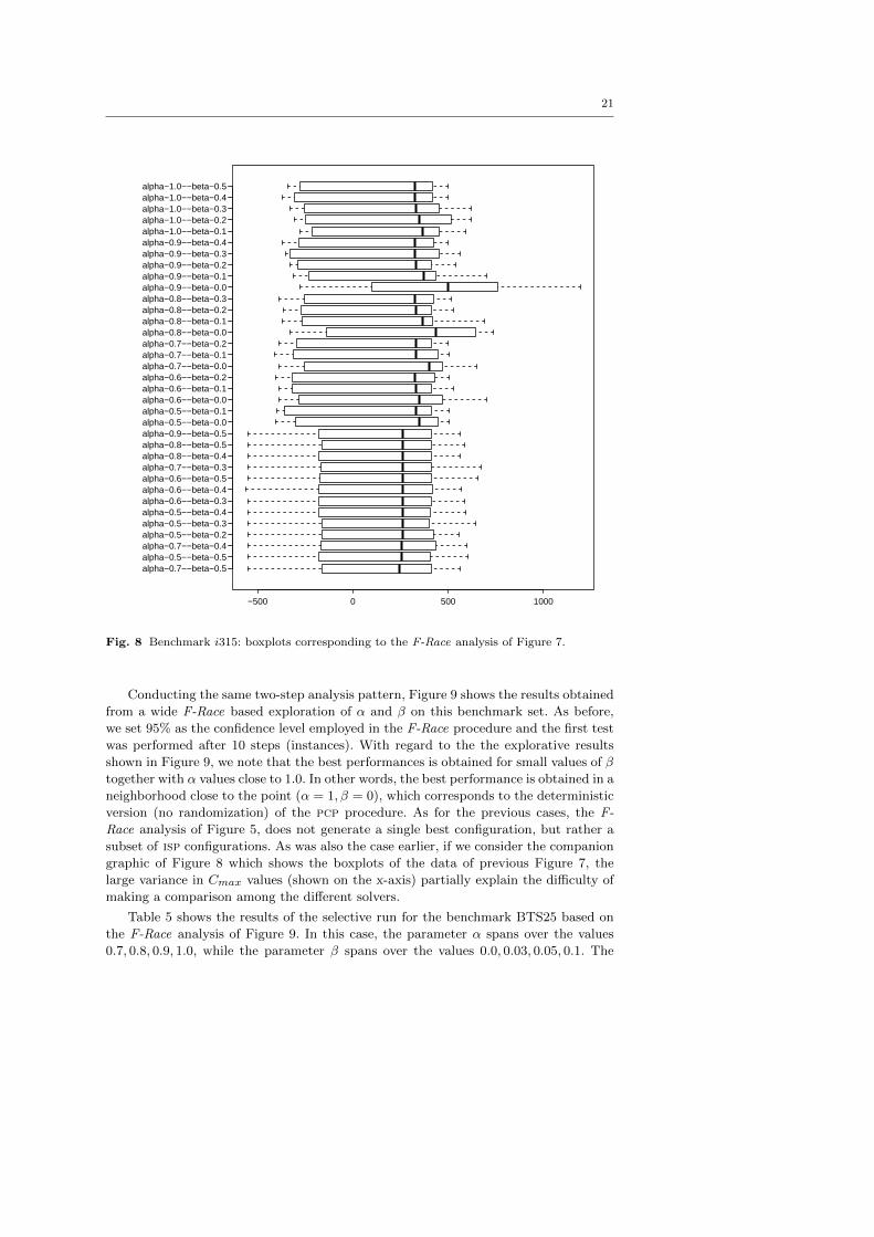
Fig. 8 Benchmark i315: boxplots corresponding to the F-Race analysis of Figure 7.

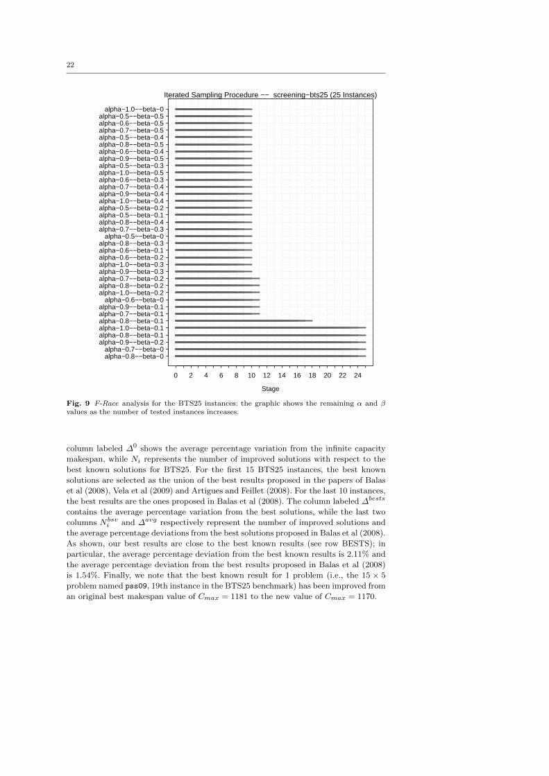
Conducting the same two-step analysis pattern, Figure 9 shows the results obtained

from a wide F-Race based exploration of α and β on this benchmark set. As before,

we set 95% as the confidence level employed in the F-Race procedure and the first test

was performed after 10 steps (instances). With regard to the the explorative results

shown in Figure 9, we note that the best performances is obtained for small values of β

together with α values close to 1.0. In other words, the best performance is obtained in a

neighborhood close to the point (α = 1, β = 0), which corresponds to the deterministic

version (no randomization) of the pcp procedure. As for the previous cases, the F-

Race analysis of Figure 5, does not generate a single best configuration, but rather a

subset of isp configurations. As was also the case earlier, if we consider the companion

graphic of Figure 8 which shows the boxplots of the data of previous Figure 7, the

large variance in Cmax values (shown on the x-axis) partially explain the difficulty of

making a comparison among the different solvers.

Table 5 shows the results of the selective run for the benchmark BTS25 based on

the F-Race analysis of Figure 9. In this case, the parameter α spans over the values

0.7, 0.8, 0.9, 1.0, while the parameter β spans over the values 0.0, 0.03, 0.05, 0.1. The

22

alpha−0.8−−beta−0alpha−0.7−−beta−0


alpha−0.6−−beta−0alpha−1.0−−beta−0.2alpha−0.8−−beta−0.2alpha−0.7−−beta−0.2alpha−0.9−−beta−0.3alpha−1.0−−beta−0.3alpha−0.6−−beta−0.2alpha−0.6−−beta−0.1alpha−0.8−−beta−0.3

alpha−0.5−−beta−0alpha−0.7−−beta−0.3alpha−0.8−−beta−0.4alpha−0.5−−beta−0.1alpha−0.5−−beta−0.2alpha−1.0−−beta−0.4alpha−0.9−−beta−0.4alpha−0.7−−beta−0.4alpha−0.6−−beta−0.3alpha−1.0−−beta−0.5alpha−0.5−−beta−0.3alpha−0.9−−beta−0.5alpha−0.6−−beta−0.4alpha−0.8−−beta−0.5alpha−0.5−−beta−0.4alpha−0.7−−beta−0.5alpha−0.6−−beta−0.5alpha−0.5−−beta−0.5

alpha−1.0−−beta−0

0 2 4 6 8 10 12 14 16 18 20 22 24

Iterated Sampling Procedure −− screening−bts25 (25 Instances)

Stage

Fig. 9 F-Race analysis for the BTS25 instances: the graphic shows the remaining α and βvalues as the number of tested instances increases.

column labeled ∆0 shows the average percentage variation from the infinite capacity

makespan, while Ni represents the number of improved solutions with respect to the

best known solutions for BTS25. For the first 15 BTS25 instances, the best known

solutions are selected as the union of the best results proposed in the papers of Balas

et al (2008), Vela et al (2009) and Artigues and Feillet (2008). For the last 10 instances,

the best results are the ones proposed in Balas et al (2008). The column labeled ∆bests

contains the average percentage variation from the best solutions, while the last two

columns Nbsvi and ∆avg respectively represent the number of improved solutions and

the average percentage deviations from the best solutions proposed in Balas et al (2008).

As shown, our best results are close to the best known results (see row BESTS); in

particular, the average percentage deviation from the best known results is 2.11% and

the average percentage deviation from the best results proposed in Balas et al (2008)

is 1.54%. Finally, we note that the best known result for 1 problem (i.e., the 15 × 5

problem named pss09, 19th instance in the BTS25 benchmark) has been improved from

an original best makespan value of Cmax = 1181 to the new value of Cmax = 1170.

23

alpha−0.8−−beta−0alpha−0.9−−beta−0.2

alpha−0.7−−beta−0alpha−0.8−−beta−0.1alpha−1.0−−beta−0.1

alpha−0.5−−beta−0alpha−0.5−−beta−0.1alpha−0.5−−beta−0.2alpha−0.5−−beta−0.3alpha−0.5−−beta−0.4alpha−0.5−−beta−0.5

alpha−0.6−−beta−0alpha−0.6−−beta−0.1alpha−0.6−−beta−0.2alpha−0.6−−beta−0.3alpha−0.6−−beta−0.4alpha−0.6−−beta−0.5alpha−0.7−−beta−0.1alpha−0.7−−beta−0.2alpha−0.7−−beta−0.3alpha−0.7−−beta−0.4alpha−0.7−−beta−0.5alpha−0.8−−beta−0.2alpha−0.8−−beta−0.3alpha−0.8−−beta−0.4alpha−0.8−−beta−0.5

alpha−0.9−−beta−0alpha−0.9−−beta−0.1alpha−0.9−−beta−0.3alpha−0.9−−beta−0.4alpha−0.9−−beta−0.5

alpha−1.0−−beta−0alpha−1.0−−beta−0.2alpha−1.0−−beta−0.3alpha−1.0−−beta−0.4alpha−1.0−−beta−0.5

800 1000 1200 1400 1600 1800

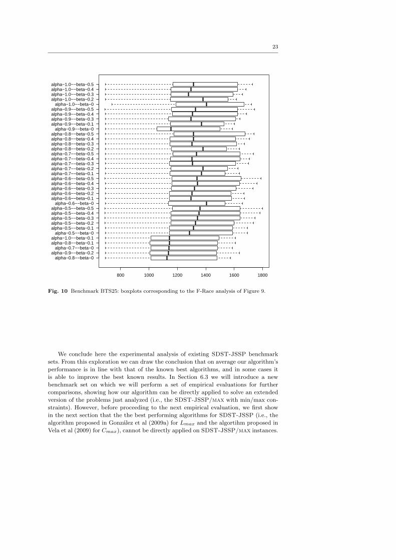
Fig. 10 Benchmark BTS25: boxplots corresponding to the F-Race analysis of Figure 9.

We conclude here the experimental analysis of existing SDST-JSSP benchmark

sets. From this exploration we can draw the conclusion that on average our algorithm’s

performance is in line with that of the known best algorithms, and in some cases it

is able to improve the best known results. In Section 6.3 we will introduce a new

benchmark set on which we will perform a set of empirical evaluations for further

comparisons, showing how our algorithm can be directly applied to solve an extended

version of the problems just analyzed (i.e., the SDST-JSSP/max with min/max con-

straints). However, before proceeding to the next empirical evaluation, we first show

in the next section that the the best performing algorithms for SDST-JSSP (i.e., the

algorithm proposed in Gonzalez et al (2009a) for Lmax and the algortihm proposed in

Vela et al (2009) for Cmax), cannot be directly applied on SDST-JSSP/max instances.

24

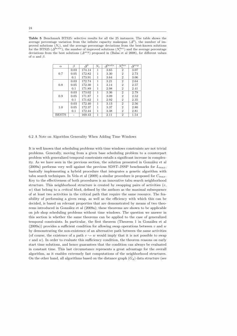
Table 5 Benchmark BTS25: selective results for all the 25 instances. The table shows theaverage percentage variation from the infinite capacity makespan (∆0), the number of im-proved solutions (Ni), and the average percentage deviations from the best-known solutionsfor the BTS25 (∆bests), the number of improved solutions (Nbsv

i ) and the average percentagedeviations from the best solutions (∆avg) proposed in (Balas et al 2008), for different valuesof α and β.

α β ∆0 Ni ∆bests Nbsvi ∆avg

0.03 174.14 1 3.65 2 3.070.7 0.05 172.82 1 3.30 2 2.73

0.1 173.91 1 3.64 2 3.060.03 172.74 1 3.21 2 2.64

0.8 0.05 172.30 1 3.14 2 2.570.1 171.89 1 2.98 2 2.410.03 173.02 1 3.36 2 2.79

0.9 0.05 171.87 1 3.09 2 2.520.1 171.62 1 2.92 2 2.350.03 172.40 1 3.13 2 2.56

1.0 0.05 172.37 1 3.37 2 2.800.1 172.44 1 3.38 2 2.81

BESTS - 169.43 1 2.11 2 1.54

6.2 A Note on Algorithm Generality When Adding Time Windows

It is well known that scheduling problems with time windows constraints are not trivial

problems. Generally, moving from a given base scheduling problem to a counterpart

problem with generalized temporal constraints entails a significant increase in complex-

ity. As we have seen in the previous section, the solution presented in Gonzalez et al

(2009a) performs very well against the previous SDST-JSSP benchmarks for Lmax,

basically implementing a hybrid procedure that integrates a genetic algorithm with

tabu search techniques. In Vela et al (2009) a similar procedure is proposed for Cmax.

Key to the effectiveness of both procedures is an innovative tabu search neighborhood

structure. This neighborhood structure is created by swapping pairs of activities (v,

w) that belong to a critical block, defined by the authors as the maximal subsequence

of at least two activities in the critical path that require the same resource. The fea-

sibility of performing a given swap, as well as the efficiency with which this can be

decided, is based on relevant properties that are demonstrated by means of two theo-

rems introduced in Gonzalez et al (2009a); these theorems are shown to be applicable

on job shop scheduling problems without time windows. The question we answer in

this section is whether the same theorems can be applied to the case of generalized

temporal constraints. In particular, the first theorem (Theorem 1 in Gonzalez et al

(2009a)) provides a sufficient condition for allowing swap operations between v and w

by demonstrating the non-existence of an alternative path between the same activities

(of course, the existence of a path v ; w would imply that it is not possible to swap

v and w). In order to evaluate this sufficiency condition, the theorem reasons on early

start time solutions, and hence guarantees that the condition can always be evaluated

in constant time. This last circumstance represents a great advantage for the overall

algorithm, as it enables extremely fast computations of the neighborhood structures.

On the other hand, all algorithms based on the distance graph (Gd) data structure (see

25

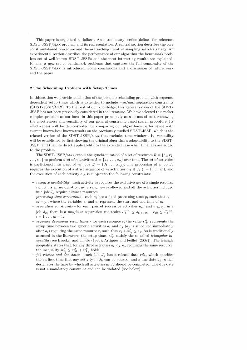
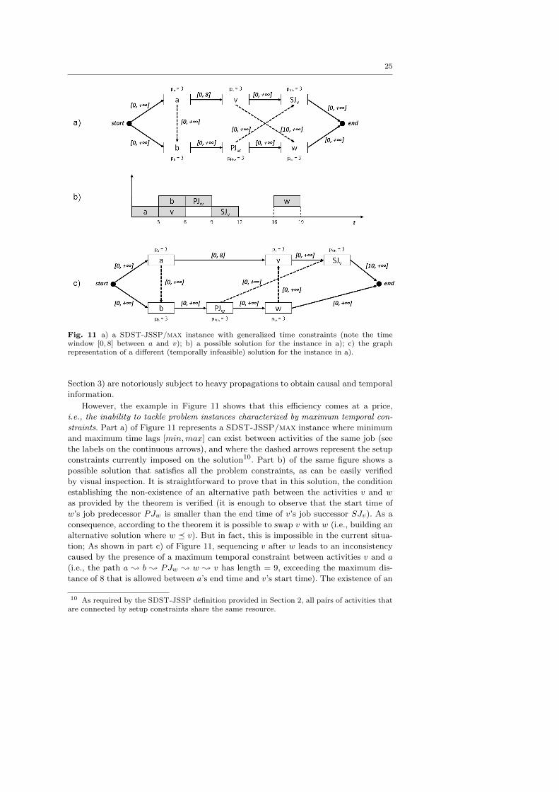
Fig. 11 a) a SDST-JSSP/max instance with generalized time constraints (note the timewindow [0, 8] between a and v); b) a possible solution for the instance in a); c) the graphrepresentation of a different (temporally infeasible) solution for the instance in a).

Section 3) are notoriously subject to heavy propagations to obtain causal and temporal

information.

However, the example in Figure 11 shows that this efficiency comes at a price,

i.e., the inability to tackle problem instances characterized by maximum temporal con-

straints. Part a) of Figure 11 represents a SDST-JSSP/max instance where minimum

and maximum time lags [min,max] can exist between activities of the same job (see

the labels on the continuous arrows), and where the dashed arrows represent the setup

constraints currently imposed on the solution10. Part b) of the same figure shows a

possible solution that satisfies all the problem constraints, as can be easily verified

by visual inspection. It is straightforward to prove that in this solution, the condition

establishing the non-existence of an alternative path between the activities v and w

as provided by the theorem is verified (it is enough to observe that the start time of

w’s job predecessor PJw is smaller than the end time of v’s job successor SJv). As a

consequence, according to the theorem it is possible to swap v with w (i.e., building an

alternative solution where w � v). But in fact, this is impossible in the current situa-

tion; As shown in part c) of Figure 11, sequencing v after w leads to an inconsistency

caused by the presence of a maximum temporal constraint between activities v and a

(i.e., the path a ; b ; PJw ; w ; v has length = 9, exceeding the maximum dis-

tance of 8 that is allowed between a’s end time and v’s start time). The existence of an

10 As required by the SDST-JSSP definition provided in Section 2, all pairs of activities thatare connected by setup constraints share the same resource.

26

alternative path between v and w escaped the theorem’s analysis because such paths

are only visible if the Gd data structure is employed. Employing this data structure

would however increase the computational burden of the procedure, and impact its

efficiency. However, without an empirical study on the adapted procedure employing

the Gd data structure, we cannot draw any reliable conclusions about the quality of

the solutions.

6.3 An Extended Benchmark and its Analysis

In order to test our procedure against SDST-JSSP/max instances, we have chosen

to create our own benchmark starting from the BTS25 benchmark described in the

previous sections. For each of the 25 original SDST-JSSP benchmark instances, a new

SDST-JSSP/max instance is constructed as follows:

1. For each original SDST-JSSP benchmark instance, a solution S = {est(ai) : i =

1 . . . n} is computed (est(ai) represents the earliest start time of the activity ai);

2. For each pair of successive activities aik and a(i+1)k in each job Jk, a min/max

separation constraint lminik ≤ s(i+1)k − eik ≤ lmax

ik is imposed, where:

lminik = 1

s δiklmaxik = sδik

where δik = est(a(i+1)k)− est(aik)− pik represents the temporal distance11, com-

puted from the solution, between the contiguous activities aik and a(i+1)k of job

Jk, and s is a positive real number.

To proceed with our analysis of the ISP procedure, we have generated two different

SDST-JSSP/max benchmarks, using two values for the s parameter, i.e., s = 1.5

and s = 2. We respectively call these benchmarks BTS25-TW15 and BTS25-TW20

(downloadable from http://pst.istc.cnr.it/~angelo/bts25tw/). From the way the

SDST-JSSP/max benchmarks are synthesized, it is clear that the smaller the value of

s, the smaller the amount slack that is allowed between any two contiguous activities

of the same job, and intuitively the resulting benchmark should be more difficult to

solve.

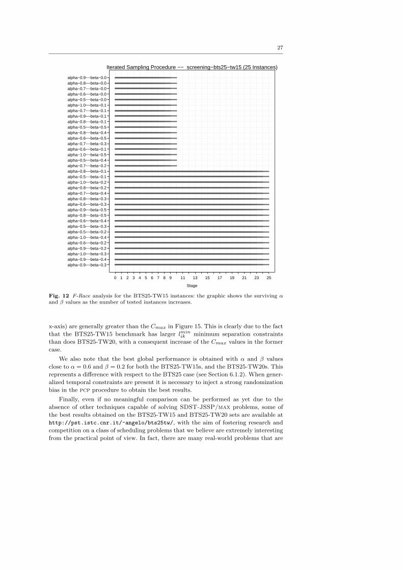
Figures 12 and 14 - and the companion boxplot graphics of Figures 13 and 15 -

respectively show the results of a F-Race analysis on BTS25-TW15s and BTS25-TW20s

for a wide range of α and β values. Even in the absence of competitors for the SDST-

JSSP/max benchmarks, a number of interesting observations can be drawn from the

previous figures. For example, in comparing both Figures 13 and 15 with Figure 10 we

observe that the Cmax values in the former are greater (i.e., entailing a worse result)

than the Cmax values in the latter. In fact, the SDST-JSSP/max benchmarks are

characterized by a greater infinite capacity makespan C0max (on average, twice as long

as their SDST-JSSP counterparts), due to the presence of minimum time lags lminik in

the job separation constraints. These increased C0max values obviously push the Cmax

values higher.

Let us now compare the results obtained in Figure 13 with those in Figure 15.

Immediately observable is the fact that the Cmax values of Figure 13 (shown on the

11 In the case δik, then we impose the separation constraint [0, 0].

27


0 1 2 3 4 5 6 7 8 9 11 13 15 17 19 21 23 25

Iterated Sampling Procedure −− screening−bts25−tw15 (25 Instances)

Stage

Fig. 12 F-Race analysis for the BTS25-TW15 instances: the graphic shows the surviving αand β values as the number of tested instances increases.

x-axis) are generally greater than the Cmax in Figure 15. This is clearly due to the fact

that the BTS25-TW15 benchmark has larger lminik minimum separation constraints

than does BTS25-TW20, with a consequent increase of the Cmax values in the former

case.

We also note that the best global performance is obtained with α and β values

close to α = 0.6 and β = 0.2 for both the BTS25-TW15s, and the BTS25-TW20s. This

represents a difference with respect to the BTS25 case (see Section 6.1.2). When gener-

alized temporal constraints are present it is necessary to inject a strong randomization

bias in the pcp procedure to obtain the best results.

Finally, even if no meaningful comparison can be performed as yet due to the

absence of other techniques capable of solving SDST-JSSP/max problems, some of

the best results obtained on the BTS25-TW15 and BTS25-TW20 sets are available at

http://pst.istc.cnr.it/~angelo/bts25tw/, with the aim of fostering research and

competition on a class of scheduling problems that we believe are extremely interesting

from the practical point of view. In fact, there are many real-world problems that are

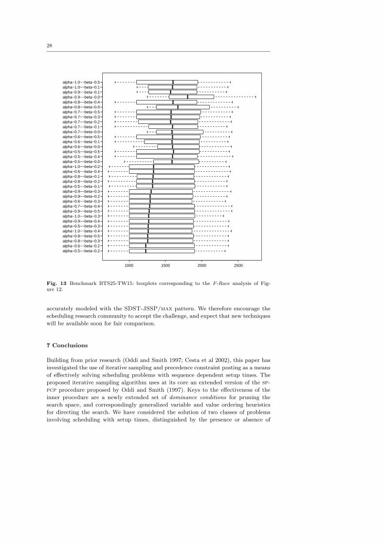
28


1000 1500 2000 2500

Fig. 13 Benchmark BTS25-TW15: boxplots corresponding to the F-Race analysis of Fig-ure 12.

accurately modeled with the SDST-JSSP/max pattern. We therefore encourage the

scheduling research community to accept the challenge, and expect that new techniques

will be available soon for fair comparison.

7 Conclusions

Building from prior research (Oddi and Smith 1997; Cesta et al 2002), this paper has

investigated the use of iterative sampling and precedence constraint posting as a means

of effectively solving scheduling problems with sequence dependent setup times. The

proposed iterative sampling algorithm uses at its core an extended version of the sp-

pcp procedure proposed by Oddi and Smith (1997). Keys to the effectiveness of the

inner procedure are a newly extended set of dominance conditions for pruning the

search space, and correspondingly generalized variable and value ordering heuristics

for directing the search. We have considered the solution of two classes of problems

involving scheduling with setup times, distinguished by the presence or absence of

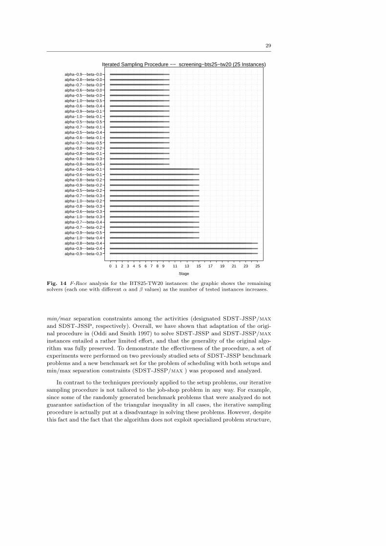
29


0 1 2 3 4 5 6 7 8 9 11 13 15 17 19 21 23 25

Iterated Sampling Procedure −− screening−bts25−tw20 (25 Instances)

Stage

Fig. 14 F-Race analysis for the BTS25-TW20 instances: the graphic shows the remainingsolvers (each one with different α and β values) as the number of tested instances increases.

min/max separation constraints among the activities (designated SDST-JSSP/max

and SDST-JSSP, respectively). Overall, we have shown that adaptation of the origi-

nal procedure in (Oddi and Smith 1997) to solve SDST-JSSP and SDST-JSSP/max

instances entailed a rather limited effort, and that the generality of the original algo-

rithm was fully preserved. To demonstrate the effectiveness of the procedure, a set of

experiments were performed on two previously studied sets of SDST-JSSP benchmark

problems and a new benchmark set for the problem of scheduling with both setups and

min/max separation constraints (SDST-JSSP/max ) was proposed and analyzed.

In contrast to the techniques previously applied to the setup problems, our iterative

sampling procedure is not tailored to the job-shop problem in any way. For example,

since some of the randomly generated benchmark problems that were analyzed do not

guarantee satisfaction of the triangular inequality in all cases, the iterative sampling

procedure is actually put at a disadvantage in solving these problems. However, despite

this fact and the fact that the algorithm does not exploit specialized problem structure,

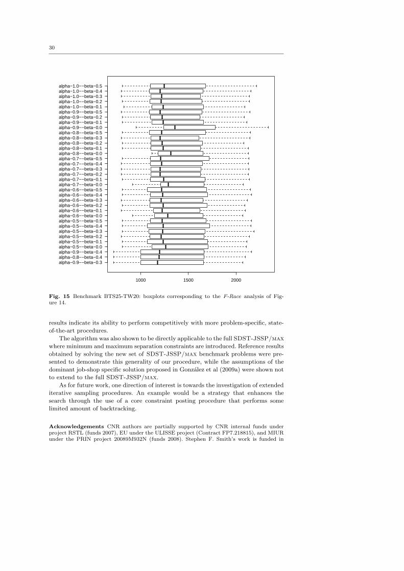
30


1000 1500 2000

Fig. 15 Benchmark BTS25-TW20: boxplots corresponding to the F-Race analysis of Fig-ure 14.

results indicate its ability to perform competitively with more problem-specific, state-

of-the-art procedures.

The algorithm was also shown to be directly applicable to the full SDST-JSSP/max

where minimum and maximum separation constraints are introduced. Reference results

obtained by solving the new set of SDST-JSSP/max benchmark problems were pre-

sented to demonstrate this generality of our procedure, while the assumptions of the

dominant job-shop specific solution proposed in Gonzalez et al (2009a) were shown not

to extend to the full SDST-JSSP/max.

As for future work, one direction of interest is towards the investigation of extended

iterative sampling procedures. An example would be a strategy that enhances the

search through the use of a core constraint posting procedure that performs some

limited amount of backtracking.

Acknowledgements CNR authors are partially supported by CNR internal funds underproject RSTL (funds 2007), EU under the ULISSE project (Contract FP7.218815), and MIURunder the PRIN project 20089M932N (funds 2008). Stephen F. Smith’s work is funded in

31

part by the US Department of Defense Advanced Research Projects Agency (DARPA) undercontract W911NF1120009 and the CMU Robotics Institute.

References

Adams J, Balas E, Zawack D (1988) The shifting bottleneck procedure for job shop scheduling.Management Science 34(3):391–401

Allahverdi A, Soroush H (2008) The significance of reducing setup times/setup costs. EuropeanJournal of Operational Research 187(3):978–984

Allahverdi A, Ng C, Cheng T, Kovalyov M (2008) A survey of scheduling problems with setuptimes or costs. European Journal of Operational Research 187(3):985–1032

Artigues C, Feillet D (2008) A branch and bound method for the job-shop problem withsequence-dependent setup times. Annals OR 159(1):135–159

Balas E, Simonetti N, Vazacopoulos A (2008) Job shop scheduling with setup times, deadlinesand precedence constraints. Journal of Scheduling 11(4):253–262

Birattari M (2010) race: Racing methods for the selection of the best. URL http://CRAN.R-project.org/package=race, r package version 0.1.58

Birattari M, Stutzle T, Paquete L, Varrentrapp K (2002) A racing algorithm for configuringmetaheuristics. In: GECCO, pp 11–18

Brucker P, Thiele O (1996) A branch & bound method for the general-shop problem withsequence dependent setup-times. OR Spectrum 18(3):145–161

Brucker P, Lenstra J, Kan AR (1977) Complexity of machine scheduling problems. Ann Dis-crete Math 1:343–362

Brucker P, Jurisch B, Sievers B (1994) A branch and bound algorithm for the job-shop schedul-ing problem. Discrete Applied Mathematics 49(1-3):107–127

Cambazard H, Hebrard E, Barry O, Papadopoulos A (2008) Local search and constraint pro-gramming for the post-enrolment-based course timetabling problem. In: PATAT ’08 – Pro-ceedings of the 7th International Conference on the Practice and Theory of AutomatedTimetabling

Cesta A, Oddi A, Smith SF (2002) A constraint-based method for project scheduling withtime windows. J Heuristics 8(1):109–136

Cheng C, Smith S (1994) Generating Feasible Schedules under Complex Metric Constraints.In: Proceedings 12th National Conference on AI (AAAI-94)

Dechter R, Meiri I, Pearl J (1991) Temporal constraint networks. Artificial Intelligence 49:61–95

Demirkol E, Mehta S, Uzsoy R (1998) Benchmarks for shop scheduling problems. EuropeanJournal of Operational Research 109(1):137–141

Focacci F, Laborie P, Nuijten W (2000) Solving scheduling problems with setup times andalternative resources. In: AIPS, pp 92–111

Gonzalez MA, Vela CR, Varela R (2009a) A Tabu Search Algorithm to Minimize Lateness inScheduling Problems with Setup Times. In: Proceedings of the CAEPIA-TTIA 2009 13thConference of the Spanish Association on Artificial Intelligence

Gonzalez MA, Vela CR, Varela R (2009b) Private CommunicationMontanari U (1974) Networks of Constraints: Fundamental Properties and Applications to

Picture Processing. Information Sciences 7:95–132Nowicki E, Smutnicki C (2005) An advanced tabu search algorithm for the job shop problem.

Journal of Scheduling 8(2):145–159Oddi A, Smith S (1997) Stochastic Procedures for Generating Feasible Schedules. In: Proceed-

ings 14th National Conference on AI (AAAI-97), pp 308–314Ovacik I, Uzsoy R (1994) Exploiting shop floor status information to schedule complex job

shops. Journal of Manufacturing Systems 13(2):73–84Ovacik I, Uzsoy R (1997) Decomposition Methods for Complex Factory Scheduling Problems.

Kluwer Academic PublishersPolicella N, Cesta A, Oddi A, Smith S (2007) From Precedence Constraint Posting to Partial

Order Schedules. AI Communications 20(3):163–180R Development Core Team (2010) R: A Language and Environment for Statistical Computing.

R Foundation for Statistical Computing, Vienna, Austria, URL http://www.R-project.org/, ISBN 3-900051-07-0

32

Sotskov YN, Shakhlevich NV (1995) Np-hardness of shop-scheduling problems with threejobs. Discrete Appl Math 59(3):237–266, DOI http://dx.doi.org/10.1016/0166-218X(93)E0169-Y

Vela CR, Varela R, Gonzalez MA (2009) Local search and genetic algorithm for the job shopscheduling problem with sequence dependent setup times. Journal of Heuristics

Documents

Solving Job Shop Scheduling with Setup Times through ... · Solving Job Shop Scheduling with Setup Times through Constraint-based Iterative Sampling: An Experimental Analysis Angelo