Digital Object Identifier (DOI) 10.1007/s10107-006-0723-7

Math. Program., Ser. B 108, 571–595 (2006)

Jorgen Blomvall · Alexander Shapiro

Solving multistage asset investment problems by the sampleaverage approximation method

Received: June 22, 2004 / Accepted: August 26, 2005Published online: June 2, 2006 – © Springer-Verlag 2006

Abstract. The vast size of real world stochastic programming instances requires sampling to make thempractically solvable. In this paper we extend the understanding of how sampling affects the solution qualityof multistage stochastic programming problems. We present a new heuristic for determining good feasiblesolutions for a multistage decision problem. For power and log-utility functions we address the question ofhow tree structures, number of stages, number of outcomes and number of assets affect the solution quality.We also present a new method for evaluating the quality of first stage decisions.

Key words. Stochastic programming – Asset allocation – Monte Carlo sampling – SAA method –Statistical bounds

1. Introduction

To fully model the complex nature of decision problems, optimization models shouldin principle contain stochastic components. Extensive research have been done withinthe field of stochastic programming to design solvers that can handle problems wherethe uncertainty is described in a tree structure. Birge and Louveaux [3] and Rusczynski[16] give a good overview of different solution methods. More recent work includes,for example, [5–7, 19] where primal and primal-dual interior point methods have beendeveloped that can solve problems with more than 2 stages and non-linear objectives.

The asset allocation problem is a frequently used stochastic programming model. Foran introduction of the model see, e.g., [12]. An excellent overview of relevant research,where the model have been applied, can be found in [13], and more recent work canbe found, e.g., in [8, 9, 2]. The model usually comes in two flavors, with and withouttransaction costs (the latter is a special case of the former). There may be also someother particularities, however, we only study the basic model.

We address several important aspects which are inherent in stochastic program-ming by studying the asset allocation model. We also test the practical applicability ofdetermining upper and lower bounds for multistage problems. For power and log-utilityfunctions, with and without transaction costs, and also for piecewise linear and expo-nential utility functions, we address how tree structures, number of stages, number ofoutcomes and number of assets affect the solution quality.

J. Blomvall: Department of Mathematics, Linkopings universitet, Linkoping, 58183 Sweden.e-mail: johan@mai.liu.se

A. Shapiro: School of Industrial and Systems Engineering, Georgia Institute of Technology, Atlanta,Georgia 30332-0205, USA. e-mail: ashapiro@isye.gatech.edu

572 J. Blomvall, A. Shapiro

2. Model

We consider an investment problem with set A of assets. For time periods t = 1, . . . , T ,the investor would like to determine the optimal amount of units ua

t of each asset a ∈ Ato buy/sell. The total units xa

t , of asset a at time t , are governed by the recursive equationsxat = xa

t−1 + uat−1, t = 2, . . . , T , where ua

t−1 can be positive or negative depending onbuying or selling asset a. By xc

t and cat we denote the amount in cash and the price of

asset a, respectively, at time t , and by R = 1 + r where r is the interest rate. Note thatcat ≥ 0. We assume that ct = (ca

t )a∈A forms a random process with a known probabilitydistribution. For the sake of simplicity we assume that the interest rate r recived in eachtime stage is fixed.

Given the initial units of assets a ∈ A, the initial amount in cash, and utility functionU(·), the objective is to maximize the expected utility of wealth, at the final time stageT . Neither short selling assets nor borrowing is allowed. This can be formulated as thefollowing optimization problem

Max E

[U

(xcT +

∑a∈A

caT xa

T

)](1)

s.t. xat = xa

t−1 + uat−1, t = 2, . . . , T , a ∈ A, (2)

xct =

(xct−1 −

∑a∈A

cat−1u

at−1

)R, t = 2, . . . , T , (3)

xat ≥ 0, t = 2, . . . , T , a ∈ A, (4)

xct ≥ 0, t = 2, . . . , T . (5)

Note that constraints (4) and (5) correspond to “not short selling assets” and “notborrowing” policies, respectively, and ensure nonnegative wealth. This will be especiallyimportant later on when sampled versions of (1–5) will be considered. If these constraintswere left out, then the optimal solution to a sample version of (1–5) might be infeasiblein the original problem. We assume that the utility function U : R → R ∪ {−∞} is acontinuous concave increasing function.

To allow for transaction costs in the model the buy/sell decision, uat , have to be split

into two variables; one for the buy decision, uabt , and one for the sell decision uas

t . Theproportional transaction cost is denoted τ . Thus the income from selling an asset is now(1−τ)ca

t and the cost of buying is (1+τ)cat for some τ ∈ (0, 1). This gives the modified

constraint (8) in the following formulation of the corresponding optimization problem

Max E

[U

(xcT +

∑a∈A

caT xa

T

)](6)

s.t. xat = xa

t−1 + uabt−1 − uas

t−1, t = 2, . . . , T , a ∈ A, (7)

xct =

(xct−1 +

∑a∈A

(τ sca

t−1uast−1 − τbca

t−1uabt−1

))R, t = 2, . . . , T , (8)

xat ≥ 0, t = 2, . . . , T , a ∈ A, (9)

xct ≥ 0, t = 2, . . . , T , (10)

Solving multistage asset investment problems 573

uabt , uas

t ≥ 0, t = 1, . . . , T − 1, a ∈ A, (11)

where τ s := 1 − τ and τb := 1 + τ .Consider the asset investment model with transaction costs. By bold script, like ca

t ,we denote random variables, while ca

t denotes a particular realization of the correspond-ing random variable. For the sake of simplicity we assume that the random processct = (ca

t )a∈A, t = 2, . . . , T , is Markovian. We also assume that xt = (xct , x

at )a∈A

satisfy linear constraints �i(xt ) ≥ 0, i ∈ I, where I is a finite index set and

�i(xt ) := αci x

ct +

∑a∈A

αai xa

t , i ∈ I.

For example, we can set �a(xt ) := xat and �c(xt ) := xc

t , with I := A ∪ {c}, whichintroduce constraints (9) and (10) into the problem.

Let us define the following cost-to-go functions. At the period T − 1 the corre-sponding cost-to-go function QT −1(xT −1, cT −1) is given by the optimal value of theproblem

MaxuT −1,xT

E

[U

(xcT +

∑a∈A

caT xa

T

) ∣∣∣∣∣cT −1 = cT −1

]

subject to xaT = xa

T −1 + uabT −1 − uas

T −1, a ∈ A,

xcT =

(xcT −1 +

∑a∈A

(τ sca

T −1uasT −1 − τbca

T −1uabT −1

))R,

uabT −1 ≥ 0, uas

T −1 ≥ 0, a ∈ A,

�i(xT ) ≥ 0, i ∈ I.

(12)

Here E[ · ∣∣ct = ct

]denotes the conditional expectation given ct = ct .

For t = T − 2, . . . , 1, the corresponding cost-to-go function Qt(xt , ct ) is defined asthe optimal value of the problem

Maxut ,xt+1

E[Qt+1(xt+1, ct+1)

∣∣ct = ct

]subject to xa

t+1 = xat + uab

t − uast , a ∈ A,

xct+1 =

(xct +

∑a∈A

(τ sca

t uast − τbca

t uabt

))R,

uabt ≥ 0, uas

t ≥ 0, a ∈ A,

�i(xt+1) ≥ 0, i ∈ I.

(13)

The optimal decision vector u1 = (uab1 , uas

1 )a∈A is obtained by solving the problem

Maxu1,x2

E [Q2(x2, c2)]

subject to xa2 = xa

1 + uab1 − uas

1 , a ∈ A,

xc2 =

(xc

1 +∑a∈A

(τ sca

1uas1 − τbca

1uab1

))R,

uab1 ≥ 0, uas

1 ≥ 0, a ∈ A,

�i(x2) ≥ 0, i ∈ I.

(14)

Note that at the first stage, vector x1 is given and (ca1)a∈A are known.

574 J. Blomvall, A. Shapiro

In the numerical experiments we assume that the asset prices cat follow a geometric

Brownian motion. That is,

ln cat = ln ca

t−1 + µa�t + σa(�t)1/2ζ at t = 2, . . . , T , a ∈ A, (15)

where random vectors ζ t = (ζ at )a∈A, t = 2, . . . , T , have normal distribution N(0, �)

with Var(ζ at ) = 1, a ∈ A, and correlations ra1a2 = E[ζ a1

t ζa2t ], and the random process

ζ t is between stages independent (i.e., random vectors ζ t , t = 2, . . . , T , are mutuallyindependent). Note that it follows from (15) and the between stages independence of ζ t ,that the process ξa

t := (cat /c

at−1)a∈A is also between stages independent.

3. Myopic policies

In practical applications quantities of interest usually are optimal values of first stagedecision variables only. In some situations, in order to obtain optimal values of firststage decision variables, one does not really need to solve the corresponding multi-stageproblem (see, e.g., [10, 1]). This is what we investigate in this section for this particularstochastic programming application.

Suppose that τ s = τb = 1, i.e., that there are no transaction costs. In that case wecan use control variables ua

t := uabt − uas

t and write the dynamic equations of (13) inthe form

uat = xa

t+1 − xat and R−1xc

t+1 +∑a∈A

cat xa

t+1 = Wt,

where Wt := xct +∑a∈A ca

t xat is the wealth at stage t . Let us make the following change

of variables:

yat+1 := ca

t xat+1, yc

t+1 := R−1xct+1 and ξa

t+1 := cat+1/c

at .

Note that this change of variables transforms the functions �i(xt+1) into the functions

li (yt+1, ct ) = (Rαc

i

)yct+1 +

∑a∈A

(αa

i /cat

)yat+1, i ∈ I,

which are linear in yt+1. We then can formulate problem (12) in the form

MaxyT

E

[U

(Ryc

T +∑a∈A

ξaT ya

T

) ∣∣∣∣∣ξT −1 = ξT −1

]

subject to ycT +

∑a∈A

yaT = WT −1,

li (yT , cT −1) ≥ 0, i ∈ I.

(1)

Let us denote by QT −1(WT −1, ξT −1) the optimal value of problem (1). Note that

QT −1 (xT −1, cT −1) = QT −1

(xcT −1 +

∑a∈A

caT −1x

aT −1, ξT −1

). (2)

Solving multistage asset investment problems 575

By continuing this process backward in time, for t = T − 2, . . . , 1, we obtain that

Qt (xt , ct ) = Qt

(xct +

∑a∈A

cat xa

t , ξt

), (3)

where Qt (Wt , ξt ) is the optimal value of the problem

Maxyt+1

E

[Qt+1

(Ryc

t+1 +∑a∈A

ξat+1y

at+1, ξ t+1

) ∣∣∣∣∣ξ t = ξt

](4)

s.t. yct+1 +

∑a∈A

yat+1 = Wt, (5)

li (yt+1, ct ) ≥ 0, i ∈ I. (6)

Note that at the first stage the wealth W1 := xc1 +∑

a∈A ca1xa

1 and asset prices ca1 are

known.Consider the set of vectors yt+1 satisfying constraints (5)–(6):

Ut (Wt , ξt ) :={

yt+1 : yct+1 +

∑a∈A

yat+1 = Wt, li(yt+1, ct ) ≥ 0, i ∈ I

}. (7)

Let us note that, since the constraints (5)–(6) are linear, the set Ut (Wt , ξt ), t = T −1, . . . , 1, is positively homogeneous with respect to Wt , i.e.,

Ut (αWt , ξt ) = α Ut (Wt , ξt ) for any α > 0. (8)

Note also that the feasible set of problem (4)–(6) should satisfy the implicit constraint

E

[Qt+1

(Ryc

t+1 +∑a∈A

ξat+1y

at+1, ξ t+1

) ∣∣∣∣∣ξ t = ξt

]> −∞. (9)

Consider now the log-utility function U(z) := log z if z > 0 and U(z) := −∞ ifz ≤ 0. We then have that

U(αz) = log α + U(z) (10)

for any α > 0 and z > 0. Since UT −1(WT −1, ξT −1) is positively homogeneous withrespect to WT −1 and because of (10), it follows that the set ST −1(WT −1, ξT −1) of

576 J. Blomvall, A. Shapiro

optimal solutions of (1) is also positively homogeneous with respect to WT −1, and forany WT −1 > 0,

QT −1(WT −1, ξT −1) = QT −1(1, ξT −1) + log WT −1. (11)

Consequently,

QT −2(WT −2, ξT −2) = E[QT −1(1, ξT −1)

∣∣ξT −2 = ξT −2]

+QT −2(WT −2, ξT −2), (12)

where QT −2(WT −2, ξT −2) is the optimal value of the problem

MaxyT −1

E

[log

(Ryc

T −1 +∑a∈A

ξaT −1y

aT −1

) ∣∣∣∣∣ξT −2 = ξT −2

]

subject to ycT −1 +

∑a∈A

yaT −1 = WT −2,

li(yT −1, cT −2) ≥ 0, i ∈ I.

(13)

Again we have that

QT −2(WT −2, ξT −2) = QT −2(1, ξT −2) + log WT −2. (14)

And so forth, for Wt > 0,

Qt (Wt , ξt ) =T −1∑τ=t

E[Qτ (1, ξ τ )

∣∣ξ t = ξt

]+ log Wt, (15)

where QT −1(WT −1, ξT −1) = QT −1(WT −1, ξT −1), and Qt (Wt , ξt ) is the optimal valueof

Maxyt+1

E

[log

(Ryc

t+1 +∑a∈A

ξat+1y

at+1

) ∣∣∣∣∣ξ t = ξt

]

subject to yct+1 +

∑a∈A

yat+1 = Wt,

li(yt+1, ct ) ≥ 0, i ∈ I,

(16)

for t = T − 2, . . . , 1. Note that if random vectors ξ t and ξ t+1 are independent, thenQt (Wt , ξt ) does not depend on ξt .

It follows that the optimal value v∗ of the corresponding (true) multistage problemis given by (recall that ξ1 = c1 and is not random)

v∗ = log W1 +T −1∑t=1

E[Qt (1, ξ t )

], (17)

Solving multistage asset investment problems 577

and first stage optimal solutions are obtained by solving the problem

Maxy2

E

[log

(Ryc

2 +∑a∈A

ξa2ya

2

)]

subject to yc2 +

∑a∈A

ya2 = W1,

li(y2, c1) ≥ 0, i ∈ I.

(18)

We obtain the following result.

Proposition 1. Suppose that there are no transaction costs and let U(·) be the log-utilityfunction. Then: (i) the optimal value v∗, of the multistage problem, is given by formula(17), (ii) the set of optimal solutions of the first stage problem (14) depends only on thedistribution of c2 (and is independent of realizations of the random data at the followingstages t = 3, . . . , T ), and can be obtained by solving problem (18).

Proof. If y2 = (yc2, y

a2 )a∈A is an optimal solution of problem (18), then

ua1 := (ca

1)−1y2a − x1

a , a ∈ A, (19)

gives the corresponding optimal solution of the first stage problem (14). Clearly the setof optimal solutions of (18) does not depend on the distribution of c3, . . . , cT . �

Remark 1. As it was mentioned above, if the process ξ t is between stages independent,then the optimal value Qt (Wt , ξt ), of problem (16), does not depend on ξt and will bedenoted Qt (Wt ). In that case formula (17) becomes

v∗ = log W1 +T −1∑t=1

Qt (1). (20)

Consider now the power utility function U(z) ≡ zγ /γ , with γ ≤ 1, γ �= 0 (in thatcase U(z) := −∞ for z ≤ 0 if γ < 0, and U(z) := −∞ for z < 0 if 0 < γ < 1).Suppose that for WT −1 = 1 problem (1) has an optimal solution yT . (The followingequation (22) can be proved without this assumption by considering an ε-optimal solu-tion, we assumed existence of the optimal solution in order to simplify the presentation.)Because of the positive homogeneity of UT −1(·, ξT −1) and since U(αz) = αγ U(z) forα > 0, we then have that WT −1yT is an optimal solution of (1) for any WT −1 > 0. Then

QT −1 (WT −1, ξT −1) = E

[U

(WT −1

(Ryc

T +∑a∈A

ξaT ya

T

)) ∣∣∣∣∣ξT −1 = ξT −1

]

= Wγ

T −1E

[U

(Ryc

T +∑a∈A

ξaT ya

T

) ∣∣∣∣∣ξT −1 = ξT −1

]

= Wγ

T −1QT −1 (1, ξT −1) . (21)

578 J. Blomvall, A. Shapiro

Suppose, further, that the random process ξ t is between stages independent. Then,because of the independence of ξT and ξT −1, we have that the conditional expecta-tion in (1) is independent of ξT −1, and hence QT −1(1, ξT −1) does not depend on ξT −1.Consequently, we obtain by (21) that for any WT −1 > 0,

QT −1 (WT −1, ξT −1) = Wγ

T −1QT −1(1), (22)

where QT −1(1) is the optimal value of (1) for WT −1 = 1. And so forth for t = T −2, . . . , 1 and Wt > 0,

Qt (Wt , ξt ) = Wγt Qt (1). (23)

Consider problems

Maxyt+1

E

[U

(Ryc

t+1 +∑a∈A

ξat+1y

at+1

)]

subject to yct+1 +

∑a∈A

yat+1 = Wt,

li(yt+1, ct ) ≥ 0, i ∈ I.

(24)

We obtain the following results.

Proposition 2. Suppose that there are no transaction costs and the random process(ξa

t = cat /c

at−1)a∈A, t = 2, . . . , T , is between stages independent, and let U(·) be the

power utility function for some γ ≤ 1, γ �= 0. Then the set of optimal solutions of thefirst stage problem (14) depends only on the distribution of ξ2 (and is independent ofrealizations of ξ3, . . . , ξT ) and can be obtained by solving problem (24) for t = 1, and

v∗ = Wγ1

T −1∏t=1

Qt (1), (25)

where Qt (Wt ) is the optimal value of the problem (24).

Remark 2. Formula (25) shows a ‘multiplicative’ behavior of the optimal value whena power utility function is used. This can be compared with an ‘additive’ behavior (see(17) and (20)) for the log-utility function. Let us also remark that the assumption of thebetween stages independence of the process ξ t is essential in the above Proposition 2.It is possible to give examples where the myopic properties of optimal solutions do nothold for the power utility functions (even for γ = 1) for stage dependent processes ξ t .This is in contrast with the log-utility function where the between stages independenceof ξ t is not needed. Let us also note that the assumption of “no transaction costs” isessential for the above myopic properties to hold.

Solving multistage asset investment problems 579

4. Solving MSP by Monte Carlo sampling

We use the following approach of conditional Monte Carlo sampling (cf., [17]). LetN = {N1, . . . , NT −1} be a sequence of positive integers. At the first stage, N1 rep-lications of the random vector c2 are generated. These replications do not need to be(stochastically) independent, it is only required that each replication has the same prob-ability distribution as c2. Then conditional on every generated realization of c2, N2replications of c3 are generated, and so forth for the following stages. In that way ascenario tree is generated with the total number of scenarios N = ∏T −1

t=1 Nt . Once suchscenario tree is generated, we can view this scenario tree as a random process with N

possible realizations (sample paths), each with equal probability 1/N . Consequently,we can associate with a generated scenario tree the optimization problem (6–11). Werefer to the obtained problem, associated with a generated sample, as the (multi-stage)sample average approximation (SAA) problem.

Provided that the sample size N is not too large, the generated SAA problem can besolved to optimality. The optimal value, denoted vN , and first stage optimal solutionsof the generated SAA problem give approximations for their counterparts of the “true”problem (6–11). (By “true” we mean the corresponding problem with the originallyspecified distribution of the random data). Note that the optimal value vN and optimalsolutions of the SAA problem depend on the generated random sample, and thereforeare random. It is possible to show that, under mild regularity conditions, the SAA esti-mators are consistent in the sense that they converge with probability one to their truecounterparts as the sample sizes Nt, t = 1, . . . , T − 1, tend to infinity (cf., [17]).

4.1. Upper statistical bounds

It is well known that

v∗ ≤ E[vN ], (1)

where v∗ denotes the optimal value of the true problem (recall that here we solve amaximization rather than a minimization problem). This gives a possibility of calculat-ing an upper statistical bound for the true optimal value v∗. This idea was suggested inNorkin, Pflug and Ruszczynski [14], and developed in Mak, Morton and Wood [11] fortwo-stage stochastic programming.

That is, SAA problems are solved (to optimality) M times for independently gener-ated samples each of size N = {N1, . . . , NT −1}. Let v1

N , . . . , vMN be calculated optimal

values of the generated SAA problems. We then have that

vN ,M := M−1M∑

j=1

vj

N (2)

is an unbiased estimator of E[vN ], and hence v∗ ≤ E[vN ,M ]. The sample variance ofvN ,M is

σ 2N ,M := 1

M(M − 1)

M∑j=1

(v

j

N − vN ,M

)2. (3)

580 J. Blomvall, A. Shapiro

This leads to the following (approximate) 100(1 − α)% confidence upper bound onE[vN ], and hence (because of (1)) for v∗:

vN ,M + tα,ν σN ,M, (4)

where ν = M −1. It should be noted that there is no reason to believe that random num-bers v

j

N have a normal (or even symmetric) distribution, even approximately, for largevalues of the sample size N . Of course, by the Central limit Theorem, the distributionof the average vN ,M approaches normal as M tends to infinity. Since the sample sizeM in the following experiments is not large, we use in (4) more conservative criticalvalues from Student’s t , rather than standard normal, distribution. One can even takeslightly larger critical values in (4) to make a correction for possibly nonsymmetricaldistribution of v

j

N .Suppose now that for a given (feasible) first stage decision vector u1, and the cor-

responding vector x2 satisfying the equations of problem (14), we want to evaluate thevalue E[Q2(x2, c2)] of the true problem. By using the developed methodology we cancalculate an upper statistical bound for E[Q2(x2, c2)] in two somewhat different ways.One, rather simple, approach is to add the constraint x2 = x2 to the correspondingoptimization problem and to use the above methodology.

Another approach can be described as follows. First, generate random sample c12, . . . ,

cN12 , of size N1, of the random vector c2. For x2 and each c

j2 , j = 1, . . . , N1, approximate

the corresponding (T − 1)-stage problem by independently generated, conditionally onc2 = c

j2 , (with a chosen sample size (N2, . . . , NT −1)) SAA problems M times. Let vj,m,

j = 1, . . . , N1, m = 1, . . . , M , be the optimal values of these SAA problems, and

¯vN1,M := 1

MN1

N1∑j=1

M∑m=1

vj,m. (5)

We have that

Q2(x2, cj2) ≤ E

[vj,m

∣∣c2 = cj2

], j = 1, . . . , N1, m = 1, . . . , M, (6)

and hence (viewing cj2 as random variables)

E[Q2(x2, c2)] = N−11

N1∑j=1

E

[Q2(x2, c

j2)

]≤ E[ ¯vN1,M ]. (7)

We can estimate the variance of ¯vN1,M as follows. Recall that if X and Y are randomvariables, then

Var(Y ) = E[Var(Y |X)] + Var[E(Y |X)], (8)

where Var(Y |X) = E[(Y − E(Y |X))2|X]. By applying this formula we can write

Var(vj,m) = E

[Var(vj,m|cj

2)]

+ Var[E(vj,m|cj

2)]. (9)

Solving multistage asset investment problems 581

Consequently, we can estimate the variance of ¯vN1,M by

σ 2N1,M

: = 1

N1M(M − 1)

N1∑j=1

M∑m=1

(vj,m − ¯vj

)2

+ 1

N1(N1 − 1)

N1∑j=1

( ¯vj − ¯vN1,M

)2, (10)

where ¯vj:= M−1∑M

m=1 vj,m.This leads to the following (approximate) 100(1 − α)% confidence upper bound on

E[Q2(x2, c2)]:

¯vN1,M + zασN1,M. (11)

Note that here we use the critical value zα from standard normal, rather than t , distributionsince the total number N1M of used variables is large.

At the first glance it seems that the second approach could be advantageous sincethere we need to solve (T − 1)-stage problems as compared with solving T -stage prob-lems in the first approach. It turned out, however, in our numerical experiments that thesecond approach involved too large variances to be practically useful.

4.2. First stage solutions

Consider the model without transaction costs and with log-utility function. In that casethe problem is myopic, and optimal first stage decision variables ua

1 are given by ua1 =

xa2 − xa

1 and xa2 = ya

2 /ca1 , a ∈ A, where ya

2 are optimal solutions of the problem (18).Therefore, if one is interested only in optimal first stage decisions, the correspondingmultistage problem effectively is reduced to a two-stage problem. Consequently theaccuracy (rate of convergence) of the SAA estimates of optimal first stage decisionvariables depends on the sample size N1 while is independent of the following samplesizes N2, . . . , NT −1. Similar conclusions hold in the case of a power utility function andbetween stages independence of the process ξ t .

4.3. Statistical properties of the upper bounds

In this section we discuss statistical properties of the upper bounds introduced in section4.1. By (1) we have that vN is a biased upwards estimator of the optimal value v∗ ofthe true problem. In particular, we investigate how the corresponding bias behaves fordifferent sample sizes and number of stages.

Let us consider the case without transaction costs and with log-utility function.Recall that conditional on a sample point ξt , at stage t , we generate a random sam-ple ξ

jt+1 = (ξ

a,jt+1)a∈A, j = 1, . . . , Nt , of size Nt , of ξ t+1. We have then that, for

582 J. Blomvall, A. Shapiro

Wt = 1, the optimal value Qt (1, ξt ), of problem (16) is approximated by the optimalvalue Qt,Nt (1, ξt ) of the problem

Maxyt+1

1

Nt

Nt∑j=1

U

(Ryc

t+1 +∑a∈A

ξa,jt+1y

at+1

)

subject to yct+1 +

∑a∈A

yat+1 = 1,

li(yt+1, ct ) ≥ 0, i ∈ I,

(12)

with U(z) ≡ log z. The difference

Bt,Nt (ξt ) := E

[Qt,Nt (1, ξt )

]− Qt (1, ξt ) (13)

represents the bias of this sample estimate conditional on ξ t = ξt . We have that

E

[Qt,Nt (1, ξt )

]≥ Qt (1, ξt ), (14)

and hence Bt,Nt (ξt ) ≥ 0.

At stage t there are Nt = ∏tτ=1 Nτ realizations of ξ t , denoted ξ

jt , j ∈ Jt , with

|Jt | = Nt . We then have (compare with (17)) that

vN = W1 +T −1∑t=1

1

Nt

∑j∈Jt

Qt,Nt (1, ξjt )

. (15)

The bias of vN ,M is equal to the bias of vN and is given by

E[vN ,M ] − v∗ =T −1∑t=1

1

Nt

∑j∈Jt

Bt,Nt (1, ξjt )

. (16)

The situation simplifies further if we assume that the process ξ t is between stages inde-pendent. Then the optimal values Qt (1, ξt ) do not depend on ξt , t = 1, . . . , T − 1, andhence Bt,Nt (ξt ) = Bt,Nt also do not depend on ξt . Consequently in such case

E[vN ,M ] − v∗ =T −1∑t=1

Bt,Nt . (17)

It follows that under the above assumptions and for constant sample sizes Nt , the biasE[vN ,M ] − v∗ grows linearly with the number of stages.

Also because of the additive structure of the bias, given by the right hand side of(17), it is possible (in the considered case) to study asymptotic behavior of the bias byinvestigating asymptotics of each component Bt,Nt with increase of the sample size Nt .This reduces such analysis to a two-stage situation. We may refer to [18] for a discussionof asymptotics of statistical estimators in two-stage stochastic programming.

The variance of vN ,M depends on a way how conditional samples are generated.Suppose that the process ξ t is between stages independent. Under this assumption, we

Solving multistage asset investment problems 583

can use the following two strategies. We can use the same sample ξjt+1, j = 1, . . . , Nt ,

for every sample point ξt at stage t . Alternatively, we can generate independent sam-ples conditional on sample points at stage t . In both cases the bias E[vN ] − v∗ is thesame, and is equal to the right hand side of (17). Because of the between stages inde-

pendence assumption, the variances Var(Qt,Nt (1, ξ

jt ))

do not depend on j ∈ Jt , and

will be denoted Var[Qt,Nt

]. For independently generated samples, we have that all

Qt,Nt

(1, ξ

jt

), j ∈ Jt , are mutually independent and hence

Var(vN) =

T −1∑t=1

Var

[Qt,Nt

]Nt

. (18)

On the other hand for conditional samples which are generated the same, we have

Var(vN) =

T −1∑t=1

Var[Qt,Nt

]. (19)

Consider now the power utility function U(z) ≡ zγ /γ , with γ ≤ 1, γ �= 0. Assumethe “no transaction costs” model and the between stages independence condition. ByProposition 2 we have that

vN = Wγ1

T −1∏t=1

(1

Nt

Qt,Nt (1, ξjt )

), (20)

where Qt,Nt (1, ξjt ) is the optimal value of problem (12) for the considered utility func-

tion. Also because of the between stages independence condition we have that

E[vN] = W

γ1

T −1∏t=1

E

[1

Nt

Qt,Nt

(1, ξ

jt

)]= W

γ1

T −1∏t=1

(Qt (1) + Bt,Nt

), (21)

where Bt,Nt is defined the same way as in the above. It follows that

E[vN ,M

]− v∗ = Wγ1

T −1∏t=1

(Qt (1) + Bt,Nt

)− Wγ1

T −1∏t=1

Qt (1)

= v∗T −1∏t=1

(1 + Bt,Nt

Qt (1)

). (22)

For the power utility function, the above formula suggests a ‘multiplicative’ behaviorof the bias with growth of the number of stages. Of course, for ‘small’ Bt,Nt /Qt (1) and‘not too’ large T , we can use the approximation

T −1∏t=1

(1 + Bt,Nt

Qt (1)

)≈ 1 +

T −1∑t=1

Bt,Nt

Qt (1),

which suggests an approximately additive behavior of the bias for a small number ofstages T .

584 J. Blomvall, A. Shapiro

4.4. Lower statistical bounds

In order to compute a valid lower statistical bound one needs to construct an implement-able and feasible policy. Given a policy of feasible decisions yielding the wealth WT ,we have that

E [U (WT )] ≤ v∗. (23)

(Note that the expectation in the left hand side of (23) is taken with respect to the con-sidered policy. We suppress this in the notation for the sake of notational simplicity.) Byusing Monte Carlo simulations, it is straightforward to construct an unbiased estimatorof E [U (WT )]. That is, a random sample of N ′ realizations of the considered randomprocess is generated and E [U (WT )] is estimated by the corresponding average

vN ′ := 1

N ′

N ′∑j=1

U(W

jT

)(24)

(cf., [18, p. 403]). Since E[vN ′

] = E [U (WT )], we have that vN ′ gives a valid lowerstatistical bound for v∗. Of course, quality of this lower bound depends on the qualityof the corresponding feasible policy. The sample variance of vN ′ is

σ 2N ′ = 1

N ′(N ′ − 1)

N ′∑j=1

[U(W

jT

)− vN ′

]2. (25)

This leads to the following (approximate) 100(1 − α)% confidence lower bound onE [U (WT )]:

vN ′ − zασN ′ . (26)

The sample size N ′ used in numerical experiments is large, therefore we use the criticalvalue zα from the standard normal distribution.

We will now study two different approaches to determine feasible decisions. TheSAA counterpart of the “true” optimization problem (6–11) can be formulated as

Max∑i∈I

Ui(xi, ui) (27)

s.t. xi = Aixi− + Biui− + bi (28)

Cixi + Diui = di (29)

Eixi + Fiui ≥ ei . (30)

Denote {x∗i , u∗

i }i∈I as the optimal solution, and let It denote the nodes that correspondto stage t . In node i the state of the stochastic parameters is ξt ∈ R

|A|. We want to finda feasible decision, uj , to node j �∈I with the state xj , ξj .

Solving multistage asset investment problems 585

It is difficult to find a decision uj that is both good and feasible. We therefore dividethe heuristics into two steps. First, we determine a target solution that is assumed to begood ut

j , then a feasible solution, uj , is determined by solving

Minuj

12 ‖ut

j − uj‖2 (31)

s.t. xlj+ ≤ Ajxj + Bjuj + bj ≤ xu

j+ (32)

Cjxj + Djuj = dj (33)

Ejxj + Fjuj ≥ ej , (34)

where xlj+ and xu

j+ is the lower and upper bound for the state in the next stage and ‖ · ‖denotes the Euclidean norm. We will next describe two heuristics for determining thetarget decision.

A common idea in stochastic programming is to reduce a scenario tree by mergingnodes with similar states of the stochastic parameters (an approach to such scenarioreduction in a certain optimal way is discussed in [4], for example), thus giving the samedecision in these merged nodes. In a similar fashion we will use a decision from a similarnode in the new node. To get a good decision we will however also have to consider thestate of the variables, xj . Define a distance between nodes in the optimal tree and thenew node as ci = ‖x∗

i − xj‖2 +‖ξi − ξj‖2. The closest decision is now utj = u∗

k , wherek = arg mini∈It

{ci}. We denote this as the closest state.By only using the closest node to determine the decision, much of the information in

the optimal decisions is lost. There usually exist many nodes that are on approximatelythe same distance. The quality of the decision in each node can also be very bad, sincenodes in later stages usually have relatively few successors. Considering these two prop-erties we will determine the target decision as an affine combination of the decisions inthe other nodes in the same time period t, uj = ∑

i∈Itλiu

∗i . λ is determined by solving,

Minλi

∑i∈It

ciλ2i (35)

s.t.∑i∈It

λiξi = ξj , (36)

∑i∈It

λix∗i = xj , (37)

∑i∈It

λi = 1, (38)

where ci = ‖x∗i − xj‖2 + ‖ξi − ξj‖2. This problem can be reformulated as

Minλ

12λT Cλ (39)

s.t. Aλ = b, (40)

586 J. Blomvall, A. Shapiro

where C is a diagonal matrix. The optimal solution λ∗ = C−1AT (AT C−1A)−1b can bedetermined with O(nm2+m3) operations, where n = |It | and m = mξ +mx+1. The tar-get decision is defined as ut

j = ∑i∈It

λ∗i u

∗i . This method is denoted affine interpolation.

5. Numerical results

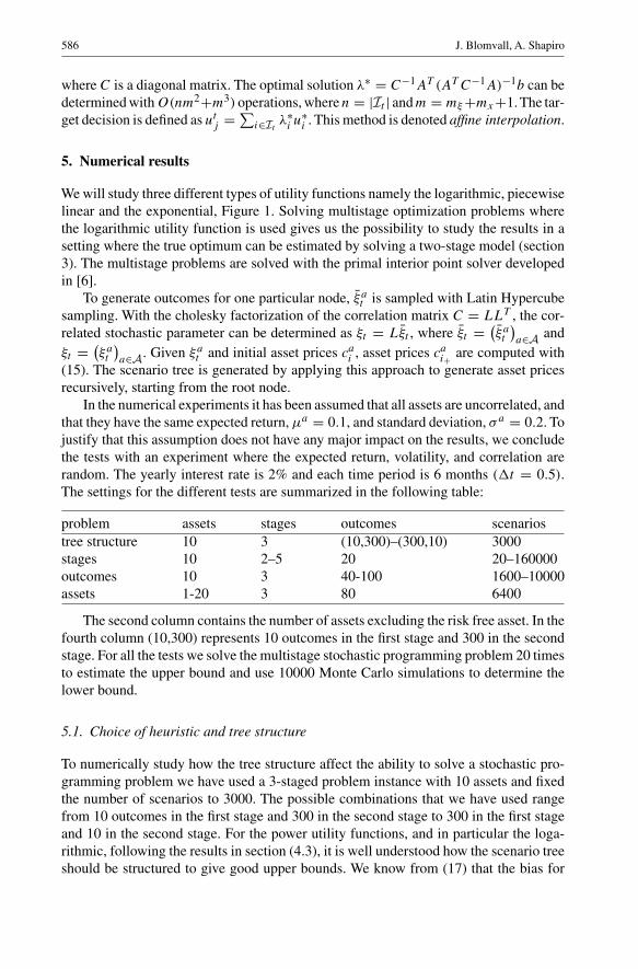
We will study three different types of utility functions namely the logarithmic, piecewiselinear and the exponential, Figure 1. Solving multistage optimization problems wherethe logarithmic utility function is used gives us the possibility to study the results in asetting where the true optimum can be estimated by solving a two-stage model (section3). The multistage problems are solved with the primal interior point solver developedin [6].

To generate outcomes for one particular node, ξ at is sampled with Latin Hypercube

sampling. With the cholesky factorization of the correlation matrix C = LLT , the cor-related stochastic parameter can be determined as ξt = Lξt , where ξt = (

ξ at

)a∈A and

ξt = (ξat

)a∈A. Given ξa

t and initial asset prices cai , asset prices ca

i+ are computed with(15). The scenario tree is generated by applying this approach to generate asset pricesrecursively, starting from the root node.

In the numerical experiments it has been assumed that all assets are uncorrelated, andthat they have the same expected return, µa = 0.1, and standard deviation, σa = 0.2. Tojustify that this assumption does not have any major impact on the results, we concludethe tests with an experiment where the expected return, volatility, and correlation arerandom. The yearly interest rate is 2% and each time period is 6 months (�t = 0.5).The settings for the different tests are summarized in the following table:

problem assets stages outcomes scenariostree structure 10 3 (10,300)–(300,10) 3000stages 10 2–5 20 20–160000outcomes 10 3 40-100 1600–10000assets 1-20 3 80 6400

The second column contains the number of assets excluding the risk free asset. In thefourth column (10,300) represents 10 outcomes in the first stage and 300 in the secondstage. For all the tests we solve the multistage stochastic programming problem 20 timesto estimate the upper bound and use 10000 Monte Carlo simulations to determine thelower bound.

5.1. Choice of heuristic and tree structure

To numerically study how the tree structure affect the ability to solve a stochastic pro-gramming problem we have used a 3-staged problem instance with 10 assets and fixedthe number of scenarios to 3000. The possible combinations that we have used rangefrom 10 outcomes in the first stage and 300 in the second stage to 300 in the first stageand 10 in the second stage. For the power utility functions, and in particular the loga-rithmic, following the results in section (4.3), it is well understood how the scenario treeshould be structured to give good upper bounds. We know from (17) that the bias for

Solving multistage asset investment problems 587

0.5 0.6 0.7 0.8 0.9 1 1.1 1.2 1.3 1.4 1.5–0.8

–0.6

–0.4

–0.2

0

0.2

0.4

0.6

Wealth

U(W

ealth

)

LogLinearExpapprox wealth pdf

Fig. 1. Objective functions used in numerical results

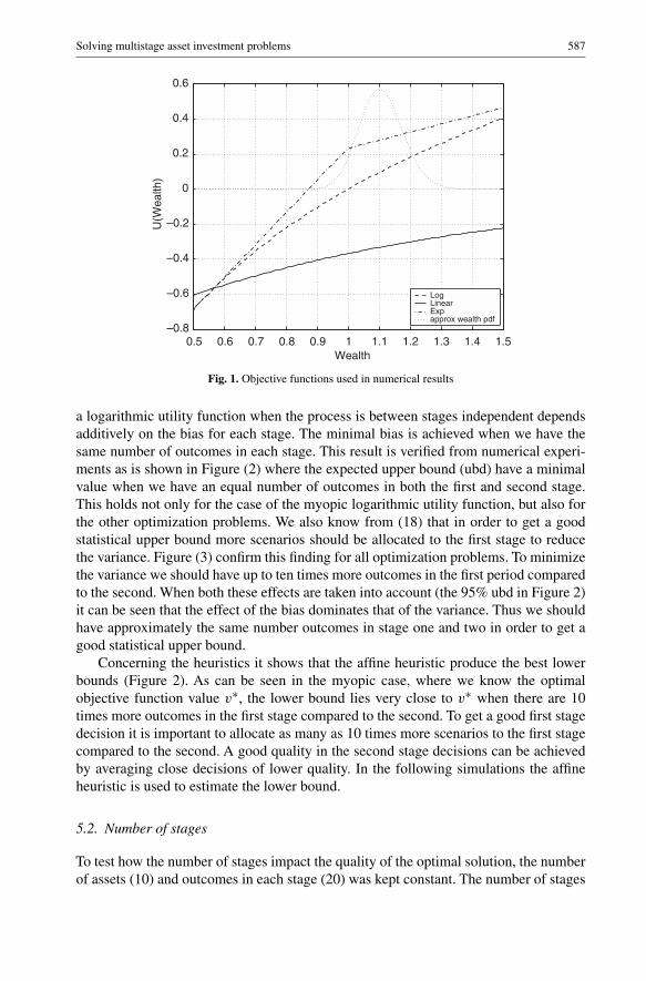
a logarithmic utility function when the process is between stages independent dependsadditively on the bias for each stage. The minimal bias is achieved when we have thesame number of outcomes in each stage. This result is verified from numerical experi-ments as is shown in Figure (2) where the expected upper bound (ubd) have a minimalvalue when we have an equal number of outcomes in both the first and second stage.This holds not only for the case of the myopic logarithmic utility function, but also forthe other optimization problems. We also know from (18) that in order to get a goodstatistical upper bound more scenarios should be allocated to the first stage to reducethe variance. Figure (3) confirm this finding for all optimization problems. To minimizethe variance we should have up to ten times more outcomes in the first period comparedto the second. When both these effects are taken into account (the 95% ubd in Figure 2)it can be seen that the effect of the bias dominates that of the variance. Thus we shouldhave approximately the same number outcomes in stage one and two in order to get agood statistical upper bound.

Concerning the heuristics it shows that the affine heuristic produce the best lowerbounds (Figure 2). As can be seen in the myopic case, where we know the optimalobjective function value v∗, the lower bound lies very close to v∗ when there are 10times more outcomes in the first stage compared to the second. To get a good first stagedecision it is important to allocate as many as 10 times more scenarios to the first stagecompared to the second. A good quality in the second stage decisions can be achievedby averaging close decisions of lower quality. In the following simulations the affineheuristic is used to estimate the lower bound.

5.2. Number of stages

To test how the number of stages impact the quality of the optimal solution, the numberof assets (10) and outcomes in each stage (20) was kept constant. The number of stages

588 J. Blomvall, A. Shapiro

10–2

10–1

100

101

102–6

–4

–2

0

2

4

6

8

10

12

# outcomes stage 1 / # outcomes stage 2

100

(v–

v*)/

v*

Expected Ubd95% UbdLbd Affine95% Lbd AffineLbd Closest95% Lbd Closest

10–2 10–1 100 101 1020.102

0.104

0.106

0.108

0.11

0.112

0.114

0.116

0.118

# outcomes stage 1 / # outcomes stage 2

v

Expected Ubd95% UbdLbd Affine95% Lbd AffineLbd Closest95% Lbd Closest

10 –2 10–1 10 0 101 10 20.27

0.275

0.28

0.285

0.29

0.295

0.3

0.305

# outcomes stage 1 / # outcomes stage 2

v

Expected Ubd95% UbdLbd Affine95% Lbd AffineLbd Closest95% Lbd Closest

10–2 10–1 100 101 1020.327

0.326

0.325

0.324

0.323

0.322

0.321

0.32

0.319

# outcomes stage 1 / # outcomes stage 2

v

Expected Ubd95% UbdLbd Affine95% Lbd AffineLbd Closest95% Lbd Closest

Fig. 2. Objective function values for different tree structures and heuristics for determining Lbd. Upper left:Scaled logarithmic utility function. Upper right: Logarithmic utility function with transaction costs. Lowerleft: Piecewise linear utility function. Lower right: Exponential utility function

10–2 10–1 100 101 10210–10

10–9

10–8

10–7

10–6

10–5

# outcomes stage 1 / # outcomes stage 2

σ2

LogLinearExpLog TransC

Fig. 3. Standard deviation of upper bounds for different tree structures

Solving multistage asset investment problems 589

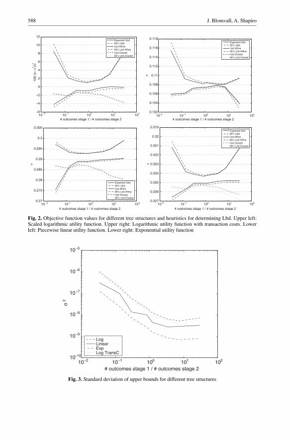
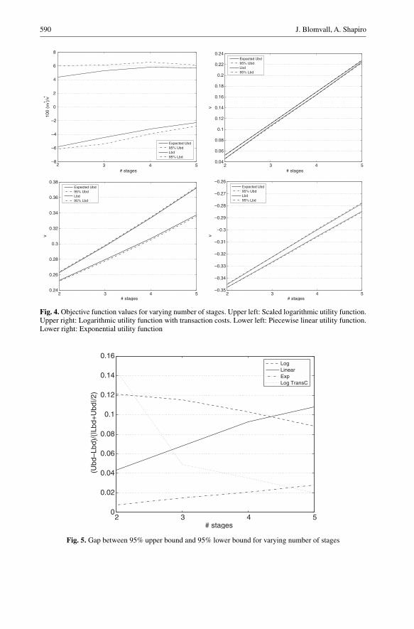
varied from 2–5, giving scenario trees with up to 160.000 scenarios. The upper left dia-gram in Figure (4) can be understood fairly well from the theory. The ratio between theaverage value of the upper bound and the optimal objective function value is essentiallyon the same level, since both the objective function value and the bias grow linearly withthe number of stages (section 4.3). Considering that the contribution to the variance ofthe upper bound is equally weighted between the number of stages the large variancefrom the first stage will have decreasing impact when the number of stages increase, thusincreasing the quality of the upper bound. A similar mechanism also improves the lowerbound. The quality of the first stage decision is bad (there are only 20 outcomes), butthe relative importance to the total objective function value decrease with an increase inthe number of stages. With this limited scenario tree one can solve a 5-staged problemand get a policy that is 3% from the optimal policy, and with a total duality gap of 9%.Figure (5) shows that the gap decrease with the number of stages for the logarithmic util-ity function both with and without transaction costs. For the case with transaction costswe use the closest policy to generate the feasible decisions in the lbd heuristic. Creatingan affine combination of decisions lead to decisions with to high transaction costs, sincein the interpolated solution both the buy and sell decisions are usually nonzero.

Overall it does not seem that the number of stages decrease the quality of the mul-tistage stochastic programming problem too much for this model, and that reasonablesolutions can be found for problems with up to 5 stages when the number of outcomesis increased.

5.3. Number of outcomes

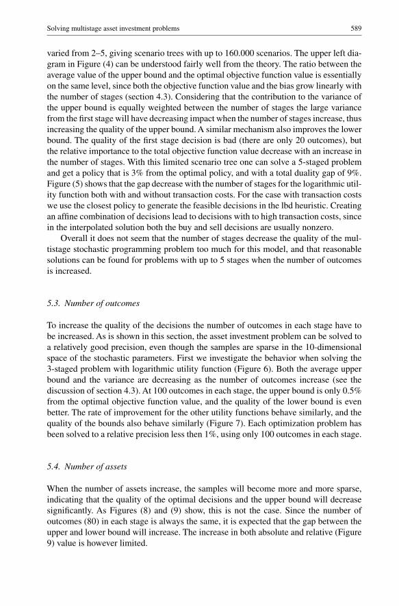
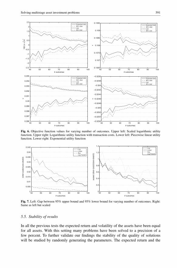
To increase the quality of the decisions the number of outcomes in each stage have tobe increased. As is shown in this section, the asset investment problem can be solved toa relatively good precision, even though the samples are sparse in the 10-dimensionalspace of the stochastic parameters. First we investigate the behavior when solving the3-staged problem with logarithmic utility function (Figure 6). Both the average upperbound and the variance are decreasing as the number of outcomes increase (see thediscussion of section 4.3). At 100 outcomes in each stage, the upper bound is only 0.5%from the optimal objective function value, and the quality of the lower bound is evenbetter. The rate of improvement for the other utility functions behave similarly, and thequality of the bounds also behave similarly (Figure 7). Each optimization problem hasbeen solved to a relative precision less then 1%, using only 100 outcomes in each stage.

5.4. Number of assets

When the number of assets increase, the samples will become more and more sparse,indicating that the quality of the optimal decisions and the upper bound will decreasesignificantly. As Figures (8) and (9) show, this is not the case. Since the number ofoutcomes (80) in each stage is always the same, it is expected that the gap between theupper and lower bound will increase. The increase in both absolute and relative (Figure9) value is however limited.

590 J. Blomvall, A. Shapiro

2 3 4 5–8

–6

–4

–2

0

2

4

6

8

# stages

100

(vv*

)/v*

Expected Ubd95% UbdLbd95% Lbd

2 3 4 50.04

0.06

0.08

0.1

0.12

0.14

0.16

0.18

0.2

0.22

0.24

# stages

v

Expected Ubd95% UbdLbd95% Lbd

2 3 4 50.24

0.26

0.28

0.3

0.32

0.34

0.36

0.38

# stages

v

Expected Ubd95% UbdLbd95% Lbd

2 3 4 5–0.35

–0.34

–0.33

–0.32

–0.31

–0.3

–0.29

–0.28

–0.27

–0.26

# stages

v

Expected Ubd95% UbdLbd95% Lbd

Fig. 4. Objective function values for varying number of stages. Upper left: Scaled logarithmic utility function.Upper right: Logarithmic utility function with transaction costs. Lower left: Piecewise linear utility function.Lower right: Exponential utility function

2 3 4 50

0.02

0.04

0.06

0.08

0.1

0.12

0.14

0.16

# stages

(Ubd

–Lbd

)/(|

Lbd+

Ubd

|/2)

LogLinearExpLog TransC

Fig. 5. Gap between 95% upper bound and 95% lower bound for varying number of stages

Solving multistage asset investment problems 591

40 50 60 70 80 90 100–2.5

–2

–1.5

–1

–0.5

0

0.5

1

1.5

2

2.5

# outcomes

100

(v–

v*)/

v*Expected Ubd95% UbdLbd95% Lbd

40 50 60 70 80 90 1000.1065

0.107

0.1075

0.108

0.1085

0.109

0.1095

# outcomes

v

Expected Ubd95% UbdLbd95% Lbd

40 50 60 70 80 90 1000.286

0.287

0.288

0.289

0.29

0.291

0.292

0.293

0.294

0.295

# outcomes

v

Expected Ubd95% UbdLbd95% Lbd

40 50 60 70 80 90 100–0.3256

–0.3254

–0.3252

–0.325

–0.3248

–0.3246

–0.3244

–0.3242

–0.324

–0.3238

–0.3236

# outcomes

v

Expected Ubd95% UbdLbd95% Lbd

Fig. 6. Objective function values for varying number of outcomes. Upper left: Scaled logarithmic utilityfunction. Upper right: Logarithmic utility function with transaction costs. Lower left: Piecewise linear utilityfunction. Lower right: Exponential utility function

40 50 60 70 80 90 1000

0.005

0.01

0.015

0.02

0.025

0.03

0.035

0.04

0.045

# outcomes

(Ubd

–Lbd

)/(|

Lbd+

Ubd

|/2)

LogLinearExpLog TransC

40 50 60 70 80 90 1000

0.2

0.4

0.6

0.8

1

1.2

1.4

# outcomes

scal

ed (

Ubd

–Lbd

)/(|

Lbd+

Ubd

|/2)

LogLinearExpLog TransC

Fig. 7. Left: Gap between 95% upper bound and 95% lower bound for varying number of outcomes. Right:Same as left but scaled

5.5. Stability of results

In all the previous tests the expected return and volatility of the assets have been equalfor all assets. With this setting many problems have been solved to a precision of afew percent. To further validate our findings the stability of the quality of solutionswill be studied by randomly generating the parameters. The expected return and the

592 J. Blomvall, A. Shapiro

0 2 4 6 8 10 12 14 16 18 20–1.5

–1

–0.5

0

0.5

1

1.5

# assets

100

(v–

v*)/

v*

Expected Ubd95% UbdLbd95% Lbd

0 2 4 6 8 10 12 14 16 18 200.085

0.09

0.095

0.1

0.105

0.11

0.115

# assets

v

Expected Ubd95% UbdLbd95% Lbd

0 2 4 6 8 10 12 14 16 18 200.25

0.255

0.26

0.265

0.27

0.275

0.28

0.285

0.29

0.295

# assets

v

Expected Ubd95% UbdLbd95% Lbd

0 2 4 6 8 10 12 14 16 18 20–0.334

–0.332

–0.33

–0.328

–0.326

–0.324

–0.322

# assets

v

Expected Ubd95% UbdLbd95% Lbd

Fig. 8. Objective function values for varying number of assets. Upper left: Scaled logarithmic utility function.Upper right: Logarithmic utility function with transaction costs. Lower left: Piecewise linear utility function.Lower right: Exponential utility function

0 2 4 6 8 10 12 14 16 18 200

0.005

0.01

0.015

0.02

0.025

# assets

(Ubd

–Lbd

)/(|

Lbd+

Ubd

|/2)

LogLinearExpLog TransC

0 2 4 6 8 10 12 14 16 18 201

2

3

4

5

6

7

8

9

# assets

scal

ed (

Ubd

–Lb

d)/(

|Lbd

+U

bd|/2

)

LogLinearExpLog TransC

Fig. 9. Left: Gap between 95% upper bound and 95% lower bound for varying number of assets. Right: Sameas left but scaled

volatility for each asset will be sampled from a rectangular probability distribution,µa ∼ Rect (0.05, 0.25) and σa ∼ Rect (0.1, 0.4). The correlation for all assets is thesame, it is sampled from a rectangular distribution, c ∼ Rect (0, 0.9). For each param-eter setting a 3-staged optimization problem is solved with 10 random assets and 100outcomes in each stage. This procedure is repeated 100 times, using the logarithmic

Solving multistage asset investment problems 593

0 0.1 0.2 0.3 0.4 0.5 0.6 0.7 0.8 0.9 10

5

10

15

20

25

100*(Ubd–Lbd)/(|Lbd+Ubd|/2)

%

Fig. 10. Histogram of gap for randomly generated µa, σ a , and ca1a2

utility function. For all these optimization problems, the quality of the solution seems tobe very stable (Figure 10). The gap between the upper and lower bound is never above1%, and the for most of the problems the gap is close to 0.7% or smaller. With the originalparameters the gap was 0.6% (Figure 7). Considering this it seems reasonable to believethat the choice of parameter values has not had any major effect on the results, and thatthe results can be assumed to hold for any asset investment problem with reasonableparameter values.

6. Evaluating the quality of first stage decisions

Suppose that we want to evaluate the quality of a given first stage decision, x2, in aT -staged decision problem. The quality of the decision can be measured by determiningthe objective function value for a T -staged optimization problem with the additionalconstraint x2 = x2 (see Section 4.1). To determine a statistical upper bound, sampledproblem instances have to be solved. The additional constraint fix the first stage decisionthus decomposing each problem instance into N1 times (T − 1)-staged subproblems.To determine a statistical lower bound several estimates are made of the total objectivefunction value. For each estimate c2 is sampled N1 times. Each resulting (T −1)-stagedproblem is solved and the outcomes contribution to the total objective function value isdetermined by simulation and affine interpolation of the decisions.

We have evaluated decisions for a 3-staged investment problem with 10 risky assets.The upper bound has been determined by 20 estimates of the objective function value andN1 = 100, N2 = 100. To estimate the lower bound, again, 20 estimates and N1 = 100are used. In each second stage node a 2-staged problem with N2 = 100 is solved and1000 simulations are made to determine the second stage objective function value. As

594 J. Blomvall, A. Shapiro

0 0.01 0.02 0.03 0.04 0.05 0.06 0.07 0.08 0.09 0.10.06

0.07

0.08

0.09

0.1

0.11

0.12

share of capital invested in each asset

v

95% Ubd95% Lbd

Fig. 11. The quality of different first stage decisions

Figure 11 shows, the quality of the first stage decision can be determined to a very highprecision. Each decision can be ordered in relation to the others in terms of quality.

7. Conclusions

For the multistage asset investment problem it is necessary to solve multistage stochasticprogramming problems whenever at least one of the following properties does not hold:

– the returns are independent– the transaction costs are zero– the utility function is of the type U(w) = wγ /γ .

For up to 5–6 stages, the multistage asset investment problem can be successfully solvedby estimating upper and lower bounds for the objective function value. This conclusionis based on a number of observations. The behavior of the upper bound for power utilityfunctions, in terms of average value and variance, is theoretically analyzed and gives agood understanding of how multistage scenario trees should be structured to provide agood upper bound. Based on the numerical experiments, it is reasonable to extend thesecharacteristics also to the other utility functions used (exponential, piecewise linear, andlogarithmic with transaction costs). By using a new heuristic to transform the decisionsin a multistage stochastic programming tree to a policy, high quality lower bounds canbe estimated. This new heuristic performs better than choosing the decision from the“closest” node.

Based on the results for generating upper and lower bounds extensive tests are madeto test how well an optimization problem with continuous random variables can be solvedwith multistage stochastic programming techniques. From the tests it can be concludedthat neither the number of stages nor the number of assets have a serious impact on the

Solving multistage asset investment problems 595

quality of the solution. It can also be concluded that the number of necessary outcomesin each time stage is rather small, in many instances a precision of 0.5% was achieved byusing only 100 outcomes in each stage. The results also seems to be stable with respectto parameter choices. The major drawback with multistage stochastic programming ishowever still present, the exponential growth of scenarios. Thus limiting the number ofstages to may be 5 or 6. These are encouraging results for users who solve multistage assetinvestment problems by stochastic programming. The stochastic programming solutionwill be reasonably close to the optimal solution, even though the number of scenariosare relatively small.

References

1. Algoet, P.H., Cover, T.M.: Asymptotic optimality and asymptotic equiparition properties of log-optimuminvestment. Ann. Probab. 16, 876–898 (1988)

2. Beltratti, A., Laurant, A., Zenios, S.A.: Scenario modelling for selective hedging strategies. J. Econ. Dyn.Control 28, 955–974 (2004)

3. Birge, J.R., Louveaux, F.: Introduction to Stochastic Programming. Springer-Verlag, New York (1997)4. Dupacova, J., Growe-Kuska, N., Romisch, W.: Scenario reduction in stochastic programming: An ap-

proach using probability metrics. Math. Program. Ser. A 95, 493–511 (2003)5. Blomvall, J.: A multistage stochastic programming algorithm suitable for parallel computing. Parallel

Comput. 29, 431–445 (2003)6. Blomvall, J., Lindberg, PO.: A Riccati-based primal interior point solver for multistage stochastic pro-

gramming. Eur. J. Oper. Res. 143, 452–461 (2002)7. Blomvall, J., Lindberg, PO.: A Riccati-based primal interior point solver for multistage stochastic pro-

gramming – extensions. Optim. Methods Softw. 17, 383–407 (2002)8. Blomvall, J., Lindberg, PO.: Back-testing the performance of an actively managed option portfolio at the

Swedish stock market, 1990–1999. J. Econ. Dyn. Control 27, 1099–1112 (2003)9. Fleten, S., Hoyland, K., Wallace, S.W.: The performance of stochastic dynamic and fixed mix portfolio

models. Eur. J. Oper. Res. 140, 37–49 (2002)10. Kelly, J.L.: A New Interpretation of Information Rate. Bell System Tech. J. 35, 917–926 (1956)11. Mak, W.K., Morton, D.P., Wood, R.K.: Monte Carlo bounding techniques for determining solution quality

in stochastic programs. Oper. Res. Lett. 24, 47–56 (1999)12. Mulvey, J.M.: Financial planning via multi-stage stochastic programs. In: J.R. Birge, K.G. Murty (eds.),

Mathematical Programming: State of the Art. University of Michigan, Ann Arbor, 1994, pp. 151–17113. Mulvey, J.M., Ziemba, W.T.: Asset and liability management systems for long-term investors: Discussion

of the issues. In: W.T. Ziemba, J.M. Mulvey (eds.), Worldwide Asset and Liability Modeling. CambridgeUniversity Press, Cambridge, 1998, pp. 1–35

14. Norkin, V.I., Pflug, G.Ch., Ruszczynski, A.: A branch and bound method for stochastic global optimiza-tion. Math. Program. 83, 425–450 (1998)

15. Pflug, G.Ch.: Scenario tree generation for multiperiod financial optimization by optimal discretization.Math. Program. Ser. B 89, 251–271 (2001)

16. Rusczynski, A.: Decomposition Methods. In: A. Rusczynski, A. Shapiro (eds.), Stochastic Programming,volume 10 of Handbooks in Operations Research and Management Science. North-Holland, 2003

17. Shapiro,A.: Statistical inference of multistage stochastic programming problems. Math. Methods of Oper.Res. 58, 57–68 (2003)

18. Shapiro, A.: Monte Carlo Sampling Methods In: A. Rusczynski, A. Shapiro (eds.), Stochastic Program-ming, volume 10 of Handbooks in Operations Research and Management Science. North-Holland, 2003

19. Steinbach, M.C.: Hierarchical sparsity in multistage convex stochastic programs. In: S.P. Uryasev,P.M. Pardalos (eds.), Stochastic Optimization: Algorithms and Applications, 385–410. Kluwer AcademicPublishers, 2001