Embed Size (px)
Citation preview
Solving Robust InventoryProblems
by
Nuri Sercan Ozbay
Submitted in partial fulfillment of the
requirements for the degree
of Doctor of Philosophy
in the Graduate School of Arts and Sciences
COLUMBIA UNIVERSITY
2006
ABSTRACT
Solving Robust Inventory Problems
In this work we consider setting the optimal inventory control policies for a single
buffer when demand is uncertain, in a robust framework. Unlike traditional inventory
models we do not assume that the demand is random with a known distribution.
Instead, demand can take values from a given uncertainty set. Our objective is to
find the policy that minimize the maximum cost that is attainable by the demand
vectors in our uncertainty set. We consider the problem for two different types of
policies which are very common in practice and present a family of algorithms based
on decomposition that scale well to problems with hundreds of time periods. We also
present theoretical results on more general models.
Contents
1 Introduction 1
1.1 Literature review . . . . . . . . . . . . . . . . . . . . . . . . . . . . . 2
1.2 Our model and contributions . . . . . . . . . . . . . . . . . . . . . . . 6
1.2.1 Generic algorithm . . . . . . . . . . . . . . . . . . . . . . . . . 11
1.3 Notation . . . . . . . . . . . . . . . . . . . . . . . . . . . . . . . . . . 14
2 The Static Problem 15
2.1 Prior work . . . . . . . . . . . . . . . . . . . . . . . . . . . . . . . . . 16
2.2 Demand uncertainty . . . . . . . . . . . . . . . . . . . . . . . . . . . 22
2.3 The decision maker’s problem . . . . . . . . . . . . . . . . . . . . . . 23
2.4 The adversarial problem under the risk budgets model . . . . . . . . 24
2.4.1 A special case . . . . . . . . . . . . . . . . . . . . . . . . . . . 29
2.4.2 The adversarial problem as a mixed-integer program . . . . . 31
2.5 The adversarial problem in the bursty demand model . . . . . . . . . 33
2.6 Computational results for the static problem . . . . . . . . . . . . . . 34
i
3 The Basestock Problem 39
3.1 Preliminaries . . . . . . . . . . . . . . . . . . . . . . . . . . . . . . . 42
3.2 The decision maker’s problem . . . . . . . . . . . . . . . . . . . . . . 44
3.3 The adversarial problem under the risk budgets model . . . . . . . . 48
3.3.1 Handling M. . . . . . . . . . . . . . . . . . . . . . . . . . . . . 53
3.3.2 Handling B. . . . . . . . . . . . . . . . . . . . . . . . . . . . . 54
3.3.3 Handling F . . . . . . . . . . . . . . . . . . . . . . . . . . . . 58
3.3.4 The algorithm . . . . . . . . . . . . . . . . . . . . . . . . . . . 58
3.3.5 The approximate adversarial algorithm . . . . . . . . . . . . . 60
3.3.6 Integral budgets case . . . . . . . . . . . . . . . . . . . . . . . 62
3.3.7 A bounding procedure for the risk budgets model . . . . . . . 63
3.4 The adversarial problem under the bursty demand model . . . . . . . 64
3.5 Experiments with the basestock model . . . . . . . . . . . . . . . . . 68
3.5.1 The risk budgets model . . . . . . . . . . . . . . . . . . . . . . 68
3.5.2 The bursty demand model . . . . . . . . . . . . . . . . . . . . 74
3.6 Extensions . . . . . . . . . . . . . . . . . . . . . . . . . . . . . . . . . 80
3.6.1 Polyhedral uncertainty sets . . . . . . . . . . . . . . . . . . . 80
3.6.2 Robust safety stocks . . . . . . . . . . . . . . . . . . . . . . . 81
3.6.3 Ambiguous uncertainty sets . . . . . . . . . . . . . . . . . . . 88
3.6.4 Model superposition . . . . . . . . . . . . . . . . . . . . . . . 91
3.6.5 More comprehensive supply-chain models . . . . . . . . . . . . 93
ii

3.7 Summary of the results . . . . . . . . . . . . . . . . . . . . . . . . . . 93
4 The Dynamic Problem 95
4.1 Preliminaries . . . . . . . . . . . . . . . . . . . . . . . . . . . . . . . 98
4.2 Characterization of optimal policies . . . . . . . . . . . . . . . . . . . 101
4.3 Risk budgets model . . . . . . . . . . . . . . . . . . . . . . . . . . . . 104
4.3.1 A special case . . . . . . . . . . . . . . . . . . . . . . . . . . . 106
4.4 Bursty demand model . . . . . . . . . . . . . . . . . . . . . . . . . . 107
Appendices 109
A An alternative approach for solving PM 109
B NP-completeness proofs 116
B.1 Proof of Theorem 3.4.1 . . . . . . . . . . . . . . . . . . . . . . . . . . 116
B.2 Proof of Theorem 3.6.1 . . . . . . . . . . . . . . . . . . . . . . . . . . 119
C Algorithms for the discrete budgets model 121
C.1 Proof of Theorem 3.6.4 . . . . . . . . . . . . . . . . . . . . . . . . . . 121
C.2 Proof of Theorem 3.6.5 . . . . . . . . . . . . . . . . . . . . . . . . . . 126
iii
List of Figures
2.1 Example with many steps . . . . . . . . . . . . . . . . . . . . . . . . 38
3.1 % error in basestock vs. % error in cost . . . . . . . . . . . . . . . . . 74
3.2 Effect of scaling peaks on optimum basestock . . . . . . . . . . . . . 79
iv
List of Tables
2.1 Solving the adversarial problem as a mixed-integer program . . . . . 32
2.2 Parameters for data generation . . . . . . . . . . . . . . . . . . . . . 35
2.3 Running time and number of iterations . . . . . . . . . . . . . . . . . 37
2.4 Running time and number of iterations for the budgets model . . . . 38
3.1 Performance of algorithm for risk budgets (T = 100). . . . . . . . . . 69
3.2 Error in the basestock produced by using early termination. . . . . . 69
3.3 Performance statistics – integral budgets . . . . . . . . . . . . . . . . 70
3.4 Ratio of adversarial time to total running time for the budgets model 71
3.5 Static vs Basestock Policies . . . . . . . . . . . . . . . . . . . . . . . 72
3.6 % increase in average cost of dynamic and static policies over the rolling
horizon basestock policy . . . . . . . . . . . . . . . . . . . . . . . . . 73
3.7 Behavior of algorithm for bursty demand model under a constant base-
stock . . . . . . . . . . . . . . . . . . . . . . . . . . . . . . . . . . . . 75
3.8 Impact of window size on a 300-period model . . . . . . . . . . . . . 76
v
3.9 Impact of initial inventory . . . . . . . . . . . . . . . . . . . . . . . . 77
3.10 Variance vs Optimal Basestock . . . . . . . . . . . . . . . . . . . . . 79
vi
CHAPTER 1. INTRODUCTION 1
Chapter 1
Introduction
Designing an efficient supply chain and operating it efficiently is one of the most im-
portant issues for a large number of modern organizations. For the past three decades,
increasing economic and competitive pressure has forced manufacturers to create bet-
ter ways to control every single step in their supply chain, from supplier contracts to
distribution channels. Due to recent fluctuations in the economy, matching supply to
demand has become even more challenging. Nowadays, there is a growing need for
more robust supply chains that are responsive to the changes in market conditions.
This work was inspired by a project carried out with an industrial partner and it con-
cerns the optimal stock ordering policies for a buffer in a supply chain in an uncertain
environment.
CHAPTER 1. INTRODUCTION 2
1.1 Literature review
The origins of Supply Chain/Inventory Management can be found as early as the
beginning of 20th century when Harris [H13] derived the Economic-Order-Quantity
formula that applies when the demand is assumed to be constant over time. Over
the few decades preceding his work numerous authors elaborated different variations
of Harris’ EOQ model. Although pioneers of the field were aware of the uncertainties
associated with the problem, the study of the problem in a stochastic setting was
only started in the 1950’s, with the seminal papers by Arrow, Harris and Marschak
[AHM51] and Dworetzky, Kiefer and Wolfowitz [DKW52]. Since then, supply chain
optimization problems have been studied extensively under stochastic settings using
different methodologies such as dynamic programming and stationary analysis. We
refer the reader to Zipkin [Z00] for a comprehensive discussion of various models in
supply chain/inventory management.
One of the most important advancements in supply chain management took place
when Clark and Scarf [CS60] proved the optimality of basestock policies for serial sys-
tems using dynamic programming, a powerful technique that would later be used by
many other authors to derive structural results about optimal inventory control poli-
cies. Subsequently, basestock policies became increasingly popular and were proved
to be optimal for many other inventory models. For further work on basestock poli-
cies see Iglehart [I63a, I63b], Veinott [V66], Ehrhart [E84] and Muharremoglu and
CHAPTER 1. INTRODUCTION 3
Tsitsiklis [MT01]. While such a policy is not necessarily optimal, it may be preferable
over optimal policies since it is easy to implement and often performs very well. Due
to its simplicity it is widely used in practice and finding optimal basestock levels itself
has drawn a lot of attention by both practitioners and researchers.
Traditional models for supply chain management are often criticized by practi-
tioners for their strong assumptions, among which is full knowledge of the underlying
demand distribution. In most real world applications, especially in industries with
short product life cycles, paucity of historical demand data makes it very hard to
determine a demand distribution that fits the observed data. In such situations the
inventory controller should make decisions using partial information, such as inaccu-
rate forecasts, about future demand, and estimates for the error in these forecasts.
To the best of our knowledge the first work on distribution free supply chain
management problems is due to Scarf [S58] who considered a single period newsvendor
problem and determined the orders that maximize the minimum expected profit over
all possible demand distributions for given first and second moments. Later, Gallego
and Moon [GM93, MG94] provided concise derivations of his results and extended
it to other cases. Gallego, Ryan and Simchi-Levi [GRS01] considered the multi-
period version of this problem with discrete demand distribution and proved the
optimality of basestock policies. Recently, Bertsimas and Thiele [BT04] and Ben-Tal
et. al. [BGNV05] studied some supply chain management problems with limited
demand information using the robust optimization framework. The central difference
CHAPTER 1. INTRODUCTION 4
of their work from previous work is that instead of assuming partial information about
the distribution of the demand, they assume that uncertain demand is explicitly
represented by a set that defines all possible demand values. In Chapter 2 we provide
a detailed discussion of their results. Also see [BGGN04] and [T05].
Robust Optimization is an increasingly accepted way to handle uncertainty. It
addresses parameter uncertainties in deterministic optimization problems. Unlike
Stochastic Programming it does not assume that the uncertain parameters are random
variables with known distributions, instead it represents uncertainty in parameters
using deterministic uncertainty sets in which all possible values of these parameters
reside. Typically, Robust Optimization adopts a min-max approach that guaran-
tees the feasibility of the obtained solution for all possible values of the uncertain
parameters in the given uncertainty sets.
Although the underlying ideas are older, the classical references for Robust Op-
timization are Ben-Tal and Nemirovski [BN98, BN99, BN00] where they studied a
group of convex optimization problems with uncertain parameters and showed that
they can be formulated as conic programs which can be solved in polynomial time.
Since then, there has been a large amount of research dealing with various aspects of
Robust Optimization. For example, Bertsimas and Sim [BS03] proposed a new poly-
hedral uncertainty set that guarantees feasibility with high probability for general
distributions for the uncertain parameters. They show that Linear Programs with
this uncertainty framework can be reformulated as Linear Programs with a small
CHAPTER 1. INTRODUCTION 5
number of additional variables. Also see [AZ05], where robustness is introduced in
the context of a combinatorial optimization problem.
Robust Optimization methodology was originally developed to deal with static
problems in which all of the decision variables are set prior to resolution of any un-
certainty. However, in most real life applications, the dynamic nature of the problems
allows decision makers to revise their decisions as more information about the uncer-
tain parameters becomes available. This is especially true for multi-period decision
making problems where static robust optimization models are unable to capture the
fact that the decision maker knows the values of uncertain parameters in the preced-
ing periods and can exploit this information when making his decisions. Recognizing
the need for incorporating the dynamic nature of the multi-period decision making
problems into Robust Optimization models, Ben-Tal et. al. [BGGN04], recently
proposed Affinely Adjustable Robust Counterpart models which feature the idea of
dynamically determining decision variables as affine functions of the portion of the
uncertain data that has been realized. By restricting the decisions to affine func-
tions of the past data they managed to produce tractable formulations for uncertain
Linear Programs. Ben-Tal et. al. [BGNV05] applied these ideas to a supply chain
management problem to get a polynomial time solvable formulation. We will review
this work more closely in Section 2.1.
Another field that deals with uncertainty in optimization problems is Adversarial
Queuing, which was first considered by Borodin et. al [BKRSW96]. They studied
CHAPTER 1. INTRODUCTION 6
packet routing over queuing networks when there is only limited information about
demand. Following an approach similar to Robust Optimization, they adopted a
worst case approach and proved some stability results that holds for all realizations
of the demand. They used a demand model that is first introduced by Cruz [C91] to
capture the burstiness of inputs in communication networks. Later, Andrews et. al.
[AAFKLL96] considered a similar problem with different network protocols.
1.2 Our model and contributions
In this thesis we develop procedures for setting the stock ordering policies for a buffer
in a supply chain subject to uncertainty in the demands. As mentioned before, our
work is motivated by experience with an industrial partner in the electronics industry
who faced the following difficulties: short product cycles, a complex supply chain
with multiple suppliers and long production leadtimes, a paucity of demand data
and a very competitive environment. The combination of these factors produced a
significant exposure to risk, in the form of either excessive inventory or shortages. The
supply chain of our industrial partner consisted of a network with multiple buffers;
however, in this work we consider a system made up of a single buffer.
We consider a buffer evolving over a finite time horizon. For t = 1, 2, . . . , T ,
the quantity xt denotes the inventory at the start of period t (possibly negative to
indicate a shortage) with x1 given. We also have a (per unit) inventory holding cost
CHAPTER 1. INTRODUCTION 7
ht, a backlogging cost bt, and a production cost ct. The dynamics during period t
work out as follows:
(a) First, one orders (produces, etc) a quantity ut ≥ 0, thereby increasing inventory
to xt + ut, and incurring a cost ctut,
(b) Next, the demand dt ≥ 0 at time t is realized, decreasing inventory to xt+1.=
xt + ut − dt,
(c) Finally, at the end of period t, we pay a cost of maxhtxt+1,−btxt+1.
This model can be extended in a number of ways, for example by considering
capacities, setup costs, or termination conditions. These features can easily be added
to the algorithms described in this thesis.
We are interested in operating the buffer so that the sum of all costs incurred
between time 1 and T is minimized. In order to devise a strategy to this effect,
we need to make precise steps (a) and (b). In what follows, we will refer to the
minimum-cost problem as the “basic inventory problem”.
In general, we are given a set D (the uncertainty set). Each element of D is a
vector (d1, d2, . . . , dT ) of demands that is available to an adversary. At time t, having
previously chosen demand values di (1 ≤ i ≤ t − 1), the adversary can choose any
demand value dt such that there is some vector (d1, . . . , dt−1, dt, dt+1, . . . , dT ) ∈ D.
Given an uncertainty set D, we need a strategy to produce orders ut so as to min-
imize the maximum cost that can arise from demands in D. To make this statement
CHAPTER 1. INTRODUCTION 8
precise, we need to specify how (a) is implemented. In other words, for each time t
we need to describe a decision rule, such that the decision maker observes the current
state of the system (e.g. the current inventory xt) and prior actions on the part of
the adversary, and chooses ut appropriately. A policy is the the sequence of such
decision rules and we denote the set of all available policies by Π. Typical examples
of policies are the basestock policy in which our decision rule in each period is given
by the function maxσt − xt for a given basestock level σt and the static policy in
which the decision maker determines the orders in advance independent of the state
of the system or actions of the adversary.
The main focus of this thesis concerns how to pick the optimal policy in the robust
setting, under various demand uncertainty sets D. In the succeeding three chapters we
consider the “basic inventory problem” for three different variants of Π. We propose
a generic methodology and using this methodology we develop algorithms to compute
the optimal stock ordering policies.
The inventory problem in the robust setting can be described as follows:
minπ∈Π
maxd∈D
cost(π, d), (1.1)
where for π ∈ Π and d ∈ D,
cost(π, d) =T∑
t=1
( ctut(π, d) + max htxt+1(π, d) , −btxt+1(π, d) ) (1.2)
where ut(π, d) denotes the order that would be placed by policy π at time t under
demands d1, d2, . . . , dt−1, and xt(π, d) would likewise denote the inventory at the start
CHAPTER 1. INTRODUCTION 9
of period t. Here, the quantity x1 (the initial inventory level) is an input and once
the demand variables (d1, d2, . . . , dt−1) ∈ D and the policy π have been chosen, ut
and xt are uniquely determined, for 1 ≤ t ≤ T . Notice that cost(π, d) is the cost
corresponding to policy π and demand pattern d; and worst-case the cost arising
from applying policy π is given by
maxd∈D
cost(π, d). (1.3)
We call (1.3) the adversarial problem.
In Section 1.2.1 we discuss a generic algorithm for solving (1.1) for different types
of policies and demand uncertainty sets (for different sets Π and D). The algorithm
is based on a common approach, Benders’ decomposition [B62], and extensive exper-
imentation shows it to be quite fast for the cases that are considered in this thesis.
Although we consider a specific inventory management problem, our methodology is
general and can be used to solve many other minmax type problems.
In Chapter 2, we limit our policy space to static policies. We assume that in each
period t, the order quantity is determined in advance and fixed regardless of the state
of the system, i.e. our decision rule is defined by a constant function of the state of the
system and the past actions by the adversary. We develop an algorithm to compute
the optimal static policy. We numerically prove the efficiency of our algorithm by
testing it on many large examples.
The static policy does not allow the inventory controller to dynamically use the
CHAPTER 1. INTRODUCTION 10
information that becomes available as the uncertainty in the system is resolved. How-
ever, this is unrealistic since in real world applications the decision maker can make
dynamic decisions. In Chapter 3 we consider the basestock policies as a tool to incor-
porate the dynamic nature of the problem into our methodology. We construct our
policy space with constant basestock policies, i.e. policies such that for 1 ≤ t ≤ T and
for a real constant σ, the order quantity in period t is equal to maxσ− xt, 0 where
xt denotes the inventory on-hand at the beginning of period t. Notice that when
using a basestock policy, the inventory controller determines an order-up-to level and
if the on-hand inventory is less that that level he places an order to push it back up
to its ideal level. Although basestock policies have their own limitations, the effect of
uncertainty on inventory levels (therefore inventory cost) is not as severe as under a
static policy because of the cap it places on inventory level. In Chapter 3 we present
a numerical comparison of optimal basestock policies with optimal static policies.
Part of the reason for our focus on basestock policies is that they have acquired
very wide use and can be shown to be optimal under stochastic inventory models.
Further, though basestock policies may not always be optimal, they are viewed as
producing easily implementable policies for practitioners. In Chapter 3 we propose
an algorithm to pick the optimal basestock level for an inventory buffer under sev-
eral robust uncertainty models. Extensive experimentation shows that our algorithm
proves to be very efficient.
At the other extreme we may consider making decisions dynamically. Instead of
CHAPTER 1. INTRODUCTION 11
determining the policy at the very beginning of the horizon, the inventory controller
can delay the ordering decision in each period t until the beginning of period t,
which makes it possible to use all of the information that becomes available by period
t. Naturally, such a policy performs very well under uncertainty since it gives the
inventory controller greater freedom to set the orders. We call this problem the
dynamic problem, and in Chapter 4 we give a characterization of the optimal policies
and show how to compute them.
1.2.1 Generic algorithm
Our generic algorithm, given next, maintains a working list D of demand patterns
– each member of D is a demand vector (d1, d2, . . . , dT ) ∈ D. The algorithm also
maintains an upper bound U and a lower bound L on the value of problem (1.1).
This algorithm can be viewed as a form of Bender’s decomposition. [B62]
Note that the decision maker’s problem is of the same general form as the generic
problem (1.1) – however, the key difference is that while D is in general exponentially
large, at any point D has size equal to the number of iterations run so far. One
of the properties of Benders’ decomposition is that, when successful, the number of
iterations until termination will be small. In experimental testing, this number turned
out quite small indeed, as we will see.
In fact, the decision maker’s problem proves to be quite tractable: roughly speak-
CHAPTER 1. INTRODUCTION 12
ing, it amounts to an easily solvable convex optimization problem. For example, in
the case of static policies the problem can be formulated as a linear program with
O(T |D|) variables and constraints.
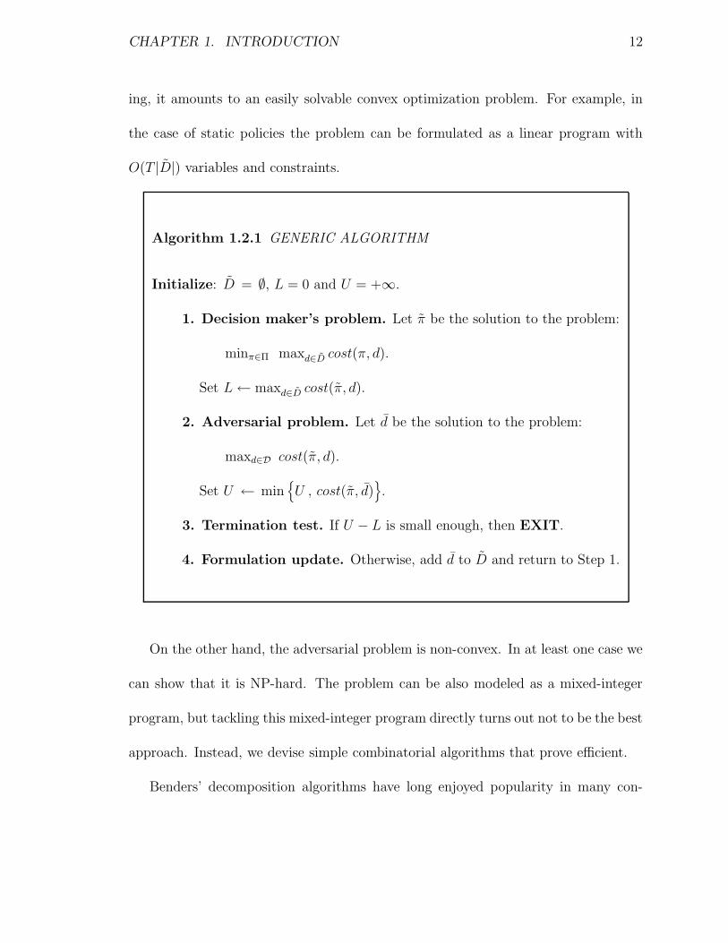
Algorithm 1.2.1 GENERIC ALGORITHM
Initialize: D = ∅, L = 0 and U = +∞.
1. Decision maker’s problem. Let π be the solution to the problem:
minπ∈Π maxd∈D cost(π, d).
Set L← maxd∈D cost(π, d).
2. Adversarial problem. Let d be the solution to the problem:
maxd∈D cost(π, d).
Set U ← min
U , cost(π, d)
.
3. Termination test. If U − L is small enough, then EXIT.
4. Formulation update. Otherwise, add d to D and return to Step 1.
On the other hand, the adversarial problem is non-convex. In at least one case we
can show that it is NP-hard. The problem can be also modeled as a mixed-integer
program, but tackling this mixed-integer program directly turns out not to be the best
approach. Instead, we devise simple combinatorial algorithms that prove efficient.
Benders’ decomposition algorithms have long enjoyed popularity in many con-
CHAPTER 1. INTRODUCTION 13
texts. In the case of stochastic programming with large number of scenarios, they
prove essential in that they effectively reduce a massively large continuous problem
into a number of much smaller independent problems. In the context of non-convex
optimization (such as the problem handled in this paper) the appeal of decomposition
is that it vastly reduces combinatorial complexity.
Benders’ decomposition methods can be viewed as a special case of cutting-plane
methods. As is the case for cutting-plane methods for combinatorial optimization,
there is no adequate general theory to explain why Benders’ decomposition, when
adequately implemented, tends to converge in few iterations. In the language of our
algorithm, part of an explanation would be that the demand patterns d added to D
in each execution of Step 4 above are “important” or “essential”, as well as being
“extremal”.
A final point regarding Algorithm 1.2.1 is that neither Step 1 nor Step 2 need be
carried out exactly, except in the last iteration (in order to prove optimality). When
either step is performed approximately, then we cannot update the corresponding
bound (U or L) as indicated in the blueprint above. However, for example, per-
forming Step 2 approximately can lead to faster iterations, and at an early stage
an approximate solution can suffice since all we are trying to do, at that point, is
to quickly improve the approximation to the set D provided by the existing (and
much smaller) set D. Our implementations run the exact adversarial problem only
at certain iterations, as will be discussed in Chapter 3.
CHAPTER 1. INTRODUCTION 14
1.3 Notation
Notation 1.3.1 In what follows, for any time period t, and any value z, we write
Wt(z) = max htz , −btz .
We will refer to the inventory holding/backlogging cost in any period as the inventory
cost.
CHAPTER 2. THE STATIC PROBLEM 15
Chapter 2
The Static Problem
In this chapter we consider the static robust inventory problem, which is defined by:
minu≥0
T∑
t=1
ctut + K(u) (2.1)
where for u = (u1, u2, . . . , uT ) ≥ 0,
K(u) = maxT∑
t=1
Wt(xt+1) (2.2)
s.t. xt+1 = xt + ut − dt, 1 ≤ t ≤ T,
(d1, d2, . . . , dT ) ∈ D.
Here (2.2) is the adversarial problem: given orders u, the adversary chooses demands
d so as to maximize the total inventory cost. We study problem (2.1) not only because
it is of interest on its own right, but because it serves as a proof-of-concept for our
basic algorithmic ideas. In addition, by running the static model at every period
CHAPTER 2. THE STATIC PROBLEM 16
in a rolling horizon fashion, we obtain a dynamic strategy, though of course not a
basestock strategy. Our algorithms are especially effective on the static problem,
solving instances with thousands of time periods in a few seconds, and consequently
extensions of the static problem should also prove efficiently solvable.
2.1 Prior work
In recent work, Bertsimas and Thiele [BT04] studied robust supply chain optimization
problems. One particular contribution lies in how they model the demand uncertainty
set D. In their model there are, for each time period t, numbers 0 ≤ δt ≤ µt and Γt,
such that 0 ≤ Γ1 ≤ Γ2 ≤ . . . ≤ ΓT and Γt ≤ Γt−1 + 1 (for 1 < t ≤ T ). A vector
of demands d is in D if and only if there exist numbers z1, z2, . . . , zT , such that for
1 ≤ t ≤ T ,
dt = µt + δtzt, (2.3)
zt ∈ [−1, 1], (2.4)
t∑
j=1
|zj| ≤ Γt. (2.5)
Here, the quantity µj is the “mean” or “nominal” demand at time j, and the model al-
lows for an absolute deviation of up to δj units away from the mean. Constraints (2.5)
constitute non-trivial requirements on the ensemble of all deviations. The method in
[BT04] handles startup costs and production capacities, but it is assumed that costs
CHAPTER 2. THE STATIC PROBLEM 17
are stationary, e.g. there are constants h, b and c such that ht = h, bt = b, and ct = c
for all t. If we extend the model in [BT04] to the general case, the approach used in
[BT04] formulates our basic inventory problem as the following linear program:
C∗ = minT∑
t=1
( ctut + yt ) (2.6)
s.t.
yt ≥ ht
x1 +t∑
j=1
(uj − µj) + At
t = 1, . . . T, (2.7)
yt ≥ bt
−x1 +t∑
j=1
(µj − uj) + At
t = 1, . . . T, (2.8)
u ≥ 0,
where for t = 1, . . . T ,
At = maxt∑
j=1
δjεtj (2.9)
s.t.t∑
j=1
εtj ≤ Γt,
0 ≤ εtj ≤ 1, 1 ≤ j ≤ t.
Thus, LP (2.9) computes the maximum cumulative deviation away from the mean
demands, by time t, that model (2.3)-(2.5) allows. If we denote by εtj (1 ≤ j ≤ t) the
optimal solution to LP (2.9), then constraint (2.7) yields the inventory holding cost
that would be incurred at time t if the demands at time 1, 2, . . . , t took values
µ1 − δ1εt1 , µ2 − δ2ε
t2 , . . . , µt − δtε
tt,
CHAPTER 2. THE STATIC PROBLEM 18
whereas constraint (2.8) yields the backlogging cost that would be incurred at time t
if the demands at time 1, 2, . . . , t took values
µ1 + δ1εt1 , µ2 + δ2ε
t2 , . . . , µt + δtε
tt,
e.g. in each case the deviations maximize the respective cost (see the discussion
following equation (13) in [BT04]). Also, note that when computing At and At′ for
t 6= t′ we will in general obtain different implied demands, e.g. εti 6= εt′
i for i ≤ t, t′.
Linear program (2.6) should be contrasted with the “true” min-max problem:
R∗ = minu≥0
R(u) (2.10)
where for u = (u1, u2, . . . , uT ) ≥ 0,
R(u) = maxd,z,x
T∑
t=1
( ctut + max htxt+1 , −btxt+1 ) (2.11)
s.t.
xt+1 = xt + ut − dt, 1 ≤ t ≤ T,
dt = µt + δtzt,
zt ∈ [−1, 1],
t∑
j=1
|zj| ≤ Γt, 1 ≤ t ≤ T.
We have that R∗ ≤ C∗ and the gap can be large. However, [BT04] empirically shows
that in the case of stationary costs (2.6) provides an effective approximation to (2.10).
This is significant because (2.11) is a non-convex optimization problem.
CHAPTER 2. THE STATIC PROBLEM 19
In addition, again in the case of stationary costs, it is shown in [BT04] that LP
(2.6) is essentially equivalent to an inventory problem with known demands, and as
a result the solution to the LP amounts to a basestock policy with basestock σt =
µt + b−hb+h
(At−At−1), with A0 = 0. In fact, LP (2.6) can be solved “greedily” (every yt
simultaneously minimized) in the stationary case. Although the non-stationary case
is not considered in [BT04], we can say that the results from the stationary case do
not directly apply.
Next we review the results in [BGNV05] in the context of our basic inventory
problem. There are three ingredients in their model. First, motivated by prior work
[GW74], and by ideas from Control Theory [GSc71], the authors propose an affine
control algorithm. Namely, the algorithm in [BGNV05] will construct for each period
1 ≤ t ≤ T parameters αjt (0 ≤ j ≤ t− 1) and impose the control law:
ut = αt0 +
t−1∑
i=1
αtidi, (2.12)
in addition to nonnegativity of the ut (this extends the methodology described in
[BGGN04]). When used at time t, the values dj in (2.12) are the past demands.
Using (2.12), the inventory holding/backlogging cost inequalities for time t become:
yt ≥ ht
x1 +t−1∑
i=1
t∑
j=i+1
αji − 1
di − dt +t∑
j=1
αj0
t = 1, . . . T, (2.13)
yt ≥ bt
−x1 +t−1∑
i=1
1−t∑
j=i+1
αji
di + dt −t∑
j=1
αj0
t = 1, . . . T, (2.14)
In addition, [BGNV05] posits that the quantities yt can be approximated (or at least,
CHAPTER 2. THE STATIC PROBLEM 20
upper-bounded) by affine functions of the past demand; the algorithm sets parameters
βtj (0 ≤ j ≤ t− 1) with yt =
∑t−1j=1 βt
jdj + βt0. Inserting this expression into (2.13), and
rearranging, we obtain:
0 ≥ htx1 +t−1∑
i=1
ht
t∑
j=i+1
αji − 1
− βti
di − htdt + ht
t∑
j=1
αj0 − βt
0, (2.15)
which can be abbreviated as
0 ≥t∑
i=1
P ti (α, β) di + P t
0(α, β), (2.16)
where each P ti (α, β) is an affine function of α and β (and similarly with (2.14)). The
algorithm in [BGNV05] chooses the α and β values so that (2.15) holds for each
demand in the uncertainty set. This set is given by dt ∈ [µt − δt , µt + δt], where
0 ≤ δt ≤ µt are known parameters. Thus, (2.16) holds for each allowable demand if
and only if there exists values νti , 1 ≤ i ≤ t, such that
0 ≥t∑
i=1
(
P ti (α, β) µi + νt
iδi
)
+ P t0(α, β), (2.17)
−νti ≤ P t
i (α, β) ≤ νti , 1 ≤ i ≤ t. (2.18)
Inequalities (2.17) and (2.18), which are linear in α, β, ν make up the system that is
enforced in [BGNV05] (there is an additional set of variables, similar to the ν, that is
used to handle the backlogging inequalities (2.14)). Notice, as was the case in [BT04],
that this approach is conservative in that we may have ν ti 6= νt′
i for some i and t 6= t′,
i.e. the demands implied by some inequality (2.17) for some t may be different from
CHAPTER 2. THE STATIC PROBLEM 21
those arising from some other period t′. Thus, the underlying min-max problem (over
the uncertainty set dt ∈ [µt − δt , µt + δt] for each t) is being approximated.
Partly in order to overcome this conservatism, [BGNV05] introduces its third
ingredient. Given that the orders and the holding/backlogging costs are represented
as affine functions of the demands, the total cost can be described as an affine function
of the demands; let us write the total cost as Q0 +∑
t Qtdt where each Qt = Qt(α, β)
is itself an affine function of α, β. To further limit the adversary, [BGNV05] models:
cost = max
Q0 +∑
t
Qtdt : d ∈ E
, where (2.19)
E = d : (d− µ)′S(d− µ) ≤ Ω . (2.20)
Here, ’ denotes transpose, S is a symmetric, positive-definite T × T matrix of known
values, Ω > 0 is given and µ is the vector of values µt. Thus, (2.20) states that the
demands cannot simultaneously take values “far” from their nominal values µt. As
shown in [BGNV05], the system (2.19), (2.20) is equivalent to the problem:
cost = min E, (2.21)
subject to: Q0 +∑
t
µtQt +(
Ω Q′ S−1 Q)1/2
− E ≤ 0. (2.22)
In this inequality, Q is the vector with entries Qt.
In summary, the approach used in [BGNV05] to handle the robust basic inventory
model solves the optimization problem with variables E, α, β and ν; with objective
CHAPTER 2. THE STATIC PROBLEM 22
(2.21), and constraints (2.22), (2.17) and (2.18) (and nonnegativity of the orders,
enforced through (2.12)). Such a problem can be efficiently solved using modern
algorithms. [BGNV05] reports excellent results in examples with T = 24.
2.2 Demand uncertainty
Here we consider the following models for the demand uncertainty set:
1. The Bertsimas-Thiele model (2.3)-(2.5). We will refer to this as the risk budgets
model. We also consider a broad generalization of this model, which we term
the intervals model.
2. Based on empirical data from our industrial partner, and borrowing ideas from
adversarial queueing theory, we consider a simple model of burstiness in demand.
In this model, each time period t is either normal or a exceptional period, and
demand arises according to the rules:
(B.a) In a normal period, we have dt ∈ [µt − δt , µt + δt], where 0 ≤ δt ≤ µt are
given parameters.
(B.b) In a exceptional period, dt = Pt, where Pt > 0 is given.
(B.c) There is a constant 0 < W ≤ T such that in any interval of W consecutive
time periods there is at most one exceptional period.
CHAPTER 2. THE STATIC PROBLEM 23
The quantities Pt are called the peaks. (B.b) and (B.c) model a severe “burst”
in demand, which is rare but does not otherwise impact the “normal” demand.
For such a model we would employ a Pt value that is “large” compared to the
normal demand, e.g. Pt = µt + 3δt. However, our approach does not make any
assumption concerning the Pt, other than Pt ≥ 0. We will refer to (B.a)-(B.c)
as the bursty demand model.
There are many possible variations of this model, for example: having several
peak types, or non-constant window parameters W . Our algorithms are easily
adapted to these models.
The risk budgets and the bursty demand model will also be considered in the context
of basestock policies and the dynamic problem. Later in the thesis we will describe
other models.
2.3 The decision maker’s problem
Step 1 of our generic algorithms requires us to solve the decision maker’s problem
for a subset of the demand uncertainty set. Let D ⊂ D. Then it is easy to see that
the decision maker’s problem for the set D can be formulated as the following linear
program.
MinT∑
t=1
(
ctut + Kdt
)
(2.23)
CHAPTER 2. THE STATIC PROBLEM 24
s.t Kdt ≥ ht(x1 +
t∑
i=1
(ui − di)) t = 1, 2, ..., T ∀ d ∈ D (2.24)
Kdt ≥ −bt(x1 +
t∑
i=1
(ui − di)) t = 1, 2, ..., T ∀ d ∈ D (2.25)
u ≥ 0 (2.26)
Here, Kdt is a variable indexed by the period, t, and the demand vector, d.
Notice that the LP above has constraints (2.24) and (2.25) for every demand
vector d ∈ D. Similarly, our main problem (2.1) can be formulated as a semi-infinite
LP by having (2.24) and (2.25) for all d ∈ D. Fortunately, (2.23)-(2.26) has a compact
representation, i.e. there exists a small subset D of D such that the LP constructed
by taking the constraints (2.24) and (2.25) corresponding to demand vectors in D will
have that same optimal solution as our semi-infinite LP. Our algorithms construct
this compact representation.
2.4 The adversarial problem under the risk bud-
gets model
Here we consider the adversarial problem (step 2 of Algorithm 1.2.1) under the de-
mand uncertainty model (2.3)-(2.5). For simplicity of presentation, in this section we
will assume that the quantities Γt are integral – in Chapter 3, where we consider the
basestock problem with the risk budgets, we will allow the Γt to be fractional. But
the integral Γt case already incorporates most of the complexity of the problem.
CHAPTER 2. THE STATIC PROBLEM 25
We have the following result:
Lemma 2.4.1 Let d be an extreme point of D. Then for 1 ≤ t ≤ T , either dt = µt
or |dt − µt| = δt.
Proof. We define zt = |dt − µt|/δt for 0 ≤ t ≤ T . Suppose that Lemma is not true
and there exist a time period t for which zt is non-integral. Let t′ be the largest such
index. Suppose∑t′
t=1 zt < Γt′ . Let ε = minΓt′ −∑t′
t=1 zt, zt′ , 1 − zt′. We form two
demand patterns d1 and d2 by setting d1t′ = dt′ − εδt′ , d2
t′ = dt′ + εδt′ and d1t = d2
t = dt.
Note that d1, d2 ∈ D and d = d1+d2
2which contradicts with the fact that d is an
extreme point of D.
Suppose that∑t′
t=1 zt = Γt′ . This means that there exists an index 1 ≤ t < t′ such
that zt is fractional. Let t′′ be the largest such index. Note that∑t
t=1 zt < Γt for
every t′′ ≤ t < t′. We set
ε = minΓt′′ −t′′∑
t=1
zt, ..., Γt′−1 −t′−1∑
t=1
zt, zt′′ , zt′ , 1− zt′′ , 1− zt′.
Similar to the previous case we form two vectors d1 and d2 by setting d1t′ = dt′ − εδt′ ,
d1t′′ = dt′′ + εδt′′ , d2
t′ = dt′ + εδt′ , d2t′′ = dt′′ − εδt′′ and d1
t = d2t = dt. d1, d2 ∈ D, and
we can write d as a linear combination of d1 and d2. Therefore d is not an extreme
point.
Using this lemma, we can now devise an algorithm for the adversarial problem. Let
u be a vector of orders. In the remainder of this section we will assume that u is
CHAPTER 2. THE STATIC PROBLEM 26
fixed. For 1 ≤ t ≤ T , and for any integer k with 0 ≤ k ≤ Γt, let At(x, k) denote the
maximum cost that the adversary can attain in periods t, . . . , T , assuming starting
inventory at time t equal to x, and that k “units” of risk have been used in all periods
preceding t. Formally,
At(x, k) = maxd
T∑
j=t
Wj
x +j∑
i=1
ui −j∑
i=1
di
(2.27)
Subject toj∑
i=t
|di − µi|
δi: δi > 0
≤ Γj − k, t ≤ j ≤ T,
µj − δj ≤ dj ≤ µj + δj, t ≤ j ≤ T.
Using this notation, the value of the adversarial problem equals∑T
t=1 ctut + A1(x1, 0).
Now (2.27) amounts to a linearly constrained program (in the d variables plus some
auxiliary variables) and it is easily seen that the demand vector that attains the max-
imum in A1(x1, 0) is an extreme point of D. Thus, using Lemma 2.4.1, we have the
following recursion:
At(x, Γt) = Wt(x + ut − µt) + At+1(x + ut − µt, Γt), (2.28)
while for k < Γt,
At(x, k) = max
fut,k(x) , f d
t,k(x) , fmt,k(x)
, (2.29)
where
fut,k(x) = Wt(x + ut − µt − δt) + At+1(x + ut − µt − δt, k + 1), (2.30)
f dt,k(x) = Wt(x + ut − µt + δt) + At+1(x + ut − µt + δt, k + 1), (2.31)
fmt,k(x) = Wt(x + ut − µt) + At+1(x + ut − µt, k). (2.32)
CHAPTER 2. THE STATIC PROBLEM 27
Here we write AT+1(x, k) = 0 for all x, k As a result of equation (2.29) and the
definition of the fut,k(x), f d
t,k(x), fmt,k(x), we have:
Lemma 2.4.2 For any t and k, At(x, k) is a convex, piecewise-linear function of x.
Equations (2.28) and (2.29)-(2.32) provide a dynamic programming algorithm for
computing A1(x1, 0). In the rest of this section we provide simple details needed to
make the algorithm efficient.
We will use the following notation: the representation of a convex piecewise-linear
function f is the description of f given by the slopes and breakpoints of its pieces,
sorted in increasing order of the slopes (i.e., “left to right”).
Lemma 2.4.3 For i = 1, 2, let f i be a convex piecewise-linear function with slopes
si1 < si
2 < . . . < sim(i). Suppose that, for some q > 0, f 1 and f 2 have q pieces of
equal slope, i.e. there are q pairs 1 ≤ a ≤ m(1), 1 ≤ b ≤ m(2), such that s1a = s2
b .
Then (a) g = maxf 1, f 2 has at most m(1) + m(2) − q pieces. Furthermore (b)
given the representations of f 1 and f 2, we can compute the representation of g in
time O(m(1) + m(2)).
Proof. First we prove (b). Let v1 < v2 < . . . < vn be the sequence of all breakpoints
of f 1 and f 2, in increasing order, where n ≤ m(1) +m(2)− 2. Suppose that for some
1 ≤ i < n we have that f 1(vi) ≥ f 2(vi) and f 2(vi+1) ≥ f 1(vi+1) where at least one of
CHAPTER 2. THE STATIC PROBLEM 28
the two inequalities is strict. Then the interval [vi, vi+1] contains a breakpoint of g. In
fact, with the exception of at most two additional breakpoints involving the first and
last pieces of f 1 and f 2, every breakpoint of g arises in this form or by exchanging
the roles of f 1 and f 2. This proves (b), since given the representation of f 1 and f 2
we can compute the sorted list v1 < v2 < . . . < vn in time O(m(1) + m(2)). To prove
(a), note that any piece of g is either (part) of a piece of m(1) or m(2); thus, since g
is convex, for any pair 1 ≤ a ≤ m(1), 1 ≤ b ≤ m(2), with s1a = s2
b (= s, say) there is
at most one piece of g with slope s.
In our implementation, we use the method implicit in Lemma 2.4.3 together with
the dynamic programming recursion described above. We will present computational
experience with this algorithm later. Here we present some comments on its com-
plexity.
Note that in each equation (2.30)-(2.32) the corresponding function f ut,k, f d
t,k or fmt,k
has at most one more breakpoint than the At+1 function in that equation. Neverthe-
less, the algorithm we are presenting is, in the worst case, of complexity exponential
in T . However, this is an overly pessimistic worst-case estimate. Comparing equa-
tions (2.30) and (2.31), we see that f ut,k(x) = f d
t,k(x− 2δt). Thus, as is easy to see (see
Lemma 2.4.4 below) maxfut,k, f
dt,k has no more breakpoints than fu
t,k, which also has
at most one more breakpoint than At(x, k + 1).
Further, Lemma 2.4.3 (a) is significant in that when we consider equations (2.30)-
(2.32) we can see that, in general, the functions f u, f d and fm will have many pieces
CHAPTER 2. THE STATIC PROBLEM 29
with equal slope. In fact, in our numerical experiments, we have not seen any example
where the number of pieces ofA1(x, 0) was large. We conjecture that for broad classes
of problems our dynamic-programming procedure runs in polynomial time.
2.4.1 A special case
There is an important special case where we can prove that our algorithm is efficient.
This is the case where the demand uncertainty set is described by the condition that
dt ∈ [µt− δt , µt + δt] for each t. In terms of the risk budgets model, this is equivalent
to having Γt = t for each t. We will refer to this special case as the box model.
In this case, the extreme points of the demand uncertainty set D are particularly
simple: they satisfy dt = µt − δt or dt = µt + δt for each t. Let At(x) denote the
maximum cost that the adversary can attain in periods t, . . . , T , assuming that the
starting inventory at time t equals x. Then:
At(x) = max
fut (x) , f d
t (x)
, (2.33)
where
fut (x) = Wt(x + ut − µt − δt) + At+1(x + ut − µt − δt), (2.34)
f dt (x) = Wt(x + ut − µt + δt) + At+1(x + ut − µt + δt). (2.35)
and as before we set AT+1(x) = 0. We have, as a consequence of Lemma 2.4.3:
CHAPTER 2. THE STATIC PROBLEM 30
Lemma 2.4.4 Let f be a piecewise-linear, convex function with m pieces, and let a
be any value. Then g(x).= max f(x) , f(x + a) is convex, piecewise-linear with at
most m pieces.
Proof. This follows directly from part (a) of Lemma 2.4.3.
Corollary 2.4.5 For any t, the number of pieces in At(x) is at most T − t + 2.
Corollary 2.4.6 In the box model, the adversarial problem can be solved in time
O(T 2).
Corollary 2.4.6 is significant for the following reason. In the box case, our min-max
problem (2.1) can be written as:
minu≥0
T∑
t=1
ct ut + z (2.36)
Subject to z ≥∑
j∈J
hj
x1 +j∑
i=1
ui −j∑
i=1
di
−∑
j∈J
bj
x1 +j∑
i=1
ui −j∑
i=1
di
,
for all d ∈ D, and each partition (J, J) of 1, . . . , T ). (2.37)
This linear program has T +1 variables but 2T |D| constraints. However, by Corollary
2.4.6, we can solve the separation problem for the feasible set of the linear program in
polynomial time – hence, we can solve the min-max problem in polynomial time, as
well [GLS93]. This result is of theoretical relevance only – in the box demands case,
our generic Benders’ algorithm proves especially efficient.
CHAPTER 2. THE STATIC PROBLEM 31
2.4.2 The adversarial problem as a mixed-integer program
Even though we are using a dynamic-programming algorithm to solve the adversarial
problem, we can also use mixed-integer programming. In the following formulation u
is the given vector of orders. For each period t, there is a zero-one variable pt which
equals 1. All other variables are continuous, and the Mt are large enough constants.
maxd,x,p,I,B,z
T∑
t=1
(It + Bt) (2.38)
Subject to
for 1 ≤ t ≤ T,
xt+1 = xt + ut − dt, (2.39)
ht xt+1 ≤ It ≤ ht xt+1 + ht Mt(1− pt), (2.40)
0 ≤ It ≤ ht Mt pt, (2.41)
−bt xt+1 ≤ Bt ≤ −bt xt+1 + bt Mtpt, (2.42)
0 ≤ Bt ≤ bt Mt (1− pt), (2.43)
dt = µt + δt zt, (2.44)
pt = 0 or 1, (2.45)
t∑
j=1
|zt| ≤ Γt. (2.46)
Equations (2.40)-(2.43) imply that when if ht xt+1 > 0 then pt = 1, and when pt = 1
then It = ht xt+1 and Bt = 0; whereas if −bt xt+1 > 0 then pt = 0, and when pt = 0
CHAPTER 2. THE STATIC PROBLEM 32
then Bt = −bt xt+1 and It = 0. In order for the formulation to be valid we need to
choose the constants Mt appropriately large – however, for efficiency of solvability,
they should be chosen just large enough, and this can be done in a straightforward
fashion.
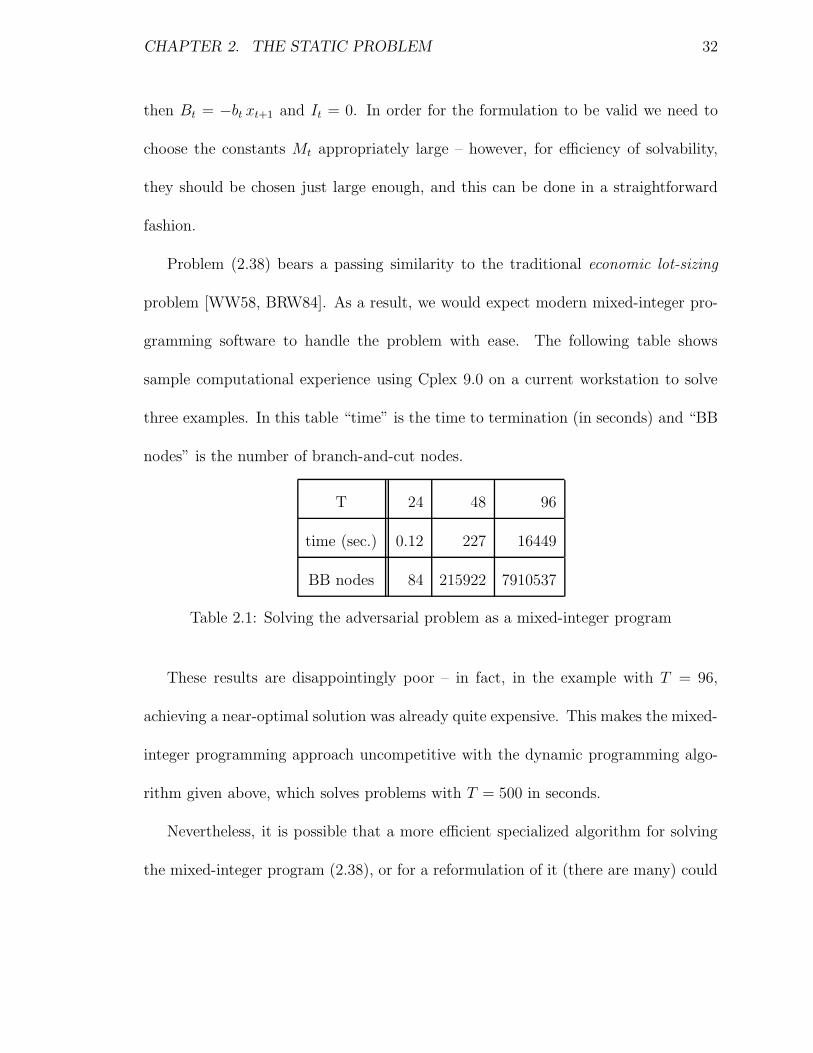
Problem (2.38) bears a passing similarity to the traditional economic lot-sizing
problem [WW58, BRW84]. As a result, we would expect modern mixed-integer pro-
gramming software to handle the problem with ease. The following table shows
sample computational experience using Cplex 9.0 on a current workstation to solve
three examples. In this table “time” is the time to termination (in seconds) and “BB
nodes” is the number of branch-and-cut nodes.
T 24 48 96
time (sec.) 0.12 227 16449
BB nodes 84 215922 7910537
Table 2.1: Solving the adversarial problem as a mixed-integer program
These results are disappointingly poor – in fact, in the example with T = 96,
achieving a near-optimal solution was already quite expensive. This makes the mixed-
integer programming approach uncompetitive with the dynamic programming algo-
rithm given above, which solves problems with T = 500 in seconds.
Nevertheless, it is possible that a more efficient specialized algorithm for solving
the mixed-integer program (2.38), or for a reformulation of it (there are many) could
CHAPTER 2. THE STATIC PROBLEM 33
be developed. In fact, notice that by replacing equation (2.46) with the general con-
dition d ∈ D we can in principle tackle the adversarial problem for general polyhedral
set D.
2.5 The adversarial problem in the bursty demand
model
Here we consider the adversarial problem for the bursty demand model given in
Section 2.2. We can adapt the dynamic programming recursion used for the risk
budgets model as follows. As previously, we assume a given vector u of orders.
For each period t, and each integer 1 ≤ k < minW, t, let Πt(x, k) denote the
maximum cost attainable by the adversary in periods t, . . . , T assuming that the initial
inventory at the start of period t is x, and that the last peak occurred in period t−k.
Similarly, denote by Πt(x, 0) the maximum cost attainable by the adversary in periods
t, . . . , T assuming that the initial inventory at the start of period t is x, and that no
peak occurred in periods t− 1, t− 2, . . . , max1, t−W + 1. Writing ΠT+1(x, k) = 0,
we have, for 1 ≤ t ≤ T :
Πt(x, k) = maxd∈µt−δt,µt+δt
Wt(x + ut − d) + Πt+1(x + ut − d, k + 1) ,
for 1 ≤ k < minW − 1, t, (2.47)
Πt(x, W − 1) = maxd∈µt−δt,µt+δt
Wt(x + ut − d) + Πt+1(x + ut − d, 0) ,
CHAPTER 2. THE STATIC PROBLEM 34
for W − 1 < t, (2.48)
Πt(x, 0) = max
Π1t (x) , Π0
t (x)
, where (2.49)
Π1t (x) = max
d∈µt−δt,µt+δtWt(x + ut − d) + Πt+1(x + ut − d, 0) , (2.50)
Π0t (x) = Wt(x + ut − Pt) + Πt+1(x + ut − Pt, 1). (2.51)
We solve this recursion using the same approach as for (2.28)-(2.32), i.e. by storing the
representation of each function Πt(x, k) (which clearly are convex piecewise-linear).
2.6 Computational results for the static problem
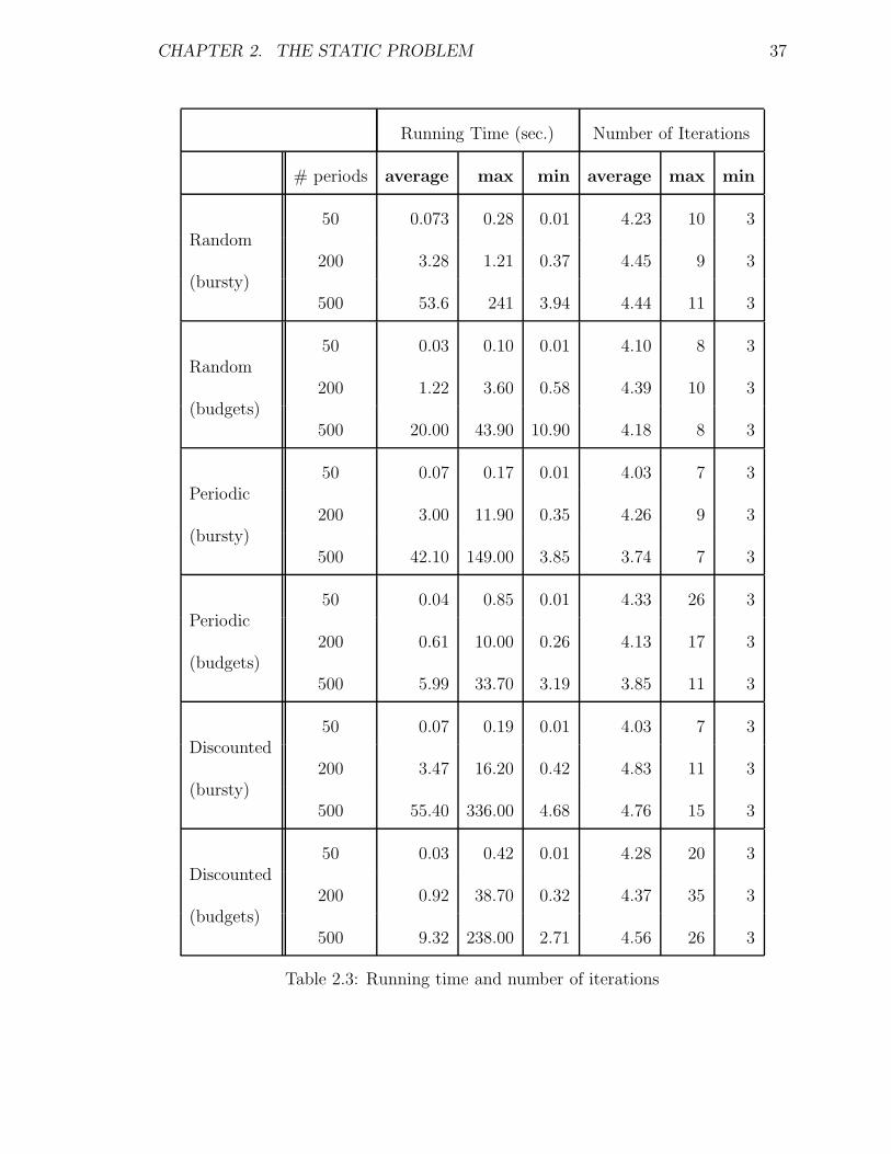
To investigate the behavior of our algorithms for the static case, we ran several sets
of tests, with results reported in Table 2.3. In this table, we report tests involving
the budgets and the bursty model of uncertainty, with three different kinds of data:
random, periodic and discounted. Further, we consider T = 50, 200, and500. We ran
500 tests for each separate category, and for each category we report the average,
maximum and minimum running time and number of steps to termination.
For all of the data types, we generate problem parameters randomly. We assume
that each period corresponds to a week and that a year has 52 weeks. In the periodic
case we generate cost parameters and demand intervals corresponding to 3 months
(13 weeks) and assume that data repeats every 3 months. For the discounted case we
generate the cost data corresponding to one period and extend this to other periods by
discounting this data using a yearly rate of 0.95. We generated the demand intervals
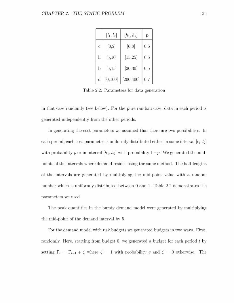
CHAPTER 2. THE STATIC PROBLEM 35
[l1, l2] [h1, h2] p
c [0,2] [6,8] 0.5
h [5,10] [15,25] 0.5
b [5,15] [20,30] 0.5
d [0,100] [200,400] 0.7
Table 2.2: Parameters for data generation
in that case randomly (see below). For the pure random case, data in each period is
generated independently from the other periods.
In generating the cost parameters we assumed that there are two possibilities. In
each period, each cost parameter is uniformly distributed either in some interval [l1, l2]
with probability p or in interval [h1, h2] with probability 1−p. We generated the mid-
points of the intervals where demand resides using the same method. The half-lengths
of the intervals are generated by multiplying the mid-point value with a random
number which is uniformly distributed between 0 and 1. Table 2.2 demonstrates the
parameters we used.
The peak quantities in the bursty demand model were generated by multiplying
the mid-point of the demand interval by 5.
For the demand model with risk budgets we generated budgets in two ways. First,
randomly. Here, starting from budget 0, we generated a budget for each period t by
setting Γt = Γt−1 + ζ where ζ = 1 with probability q and ζ = 0 otherwise. The
CHAPTER 2. THE STATIC PROBLEM 36
parameter q is likewise randomly chosen with uniform distribution.
We also tested our algorithm on stationary instances in which the budgets are
generated by the procedure given in [BT04]. Let d be a demand vector and let
C(d, Γ) be the cost of this demand vector with the optimal robust policy computed
by our algorithm for the budget vector Γ. The method in [BT04] assumes that d
is a random vector and generates the Γ vector that minimizes an upper bound on
E[C(d, Γ)] assuming that the first two moments of the distribution is given. The
algorithm gives budgets which are not necessaryly integral. We round them down,
since our algorithm for the static model can only handle the integral budget case.
These results are given in Table 2.4.
We note the low number of iterations – this shows that on average approximately
four demand patterns suffice to prove optimality (of the optimal policy). The max-
imum we observed is larger but still quite modest. In fact, Table 2.3 may overstate
the amount of work needed to converge. This is because in addition to requiring few
iterations, frequently the algorithm quickly converged to a near-optimal solution and
the additional iterations were needed in order to close a very small gap. Figure 2.1
shows a typical example of this behavior. In the figure the gap between the lower and
the upper bounds for the cost decreases rapidly and after fifth iteration we obtain a
solution that is very close to the optimal in terms of cost.
CHAPTER 2. THE STATIC PROBLEM 37
Running Time (sec.) Number of Iterations
# periods average max min average max min
Random
(bursty)
50 0.073 0.28 0.01 4.23 10 3
200 3.28 1.21 0.37 4.45 9 3
500 53.6 241 3.94 4.44 11 3
Random
(budgets)
50 0.03 0.10 0.01 4.10 8 3
200 1.22 3.60 0.58 4.39 10 3
500 20.00 43.90 10.90 4.18 8 3
Periodic
(bursty)
50 0.07 0.17 0.01 4.03 7 3
200 3.00 11.90 0.35 4.26 9 3
500 42.10 149.00 3.85 3.74 7 3
Periodic
(budgets)
50 0.04 0.85 0.01 4.33 26 3
200 0.61 10.00 0.26 4.13 17 3
500 5.99 33.70 3.19 3.85 11 3
Discounted
(bursty)
50 0.07 0.19 0.01 4.03 7 3
200 3.47 16.20 0.42 4.83 11 3
500 55.40 336.00 4.68 4.76 15 3
Discounted
(budgets)
50 0.03 0.42 0.01 4.28 20 3
200 0.92 38.70 0.32 4.37 35 3
500 9.32 238.00 2.71 4.56 26 3
Table 2.3: Running time and number of iterations
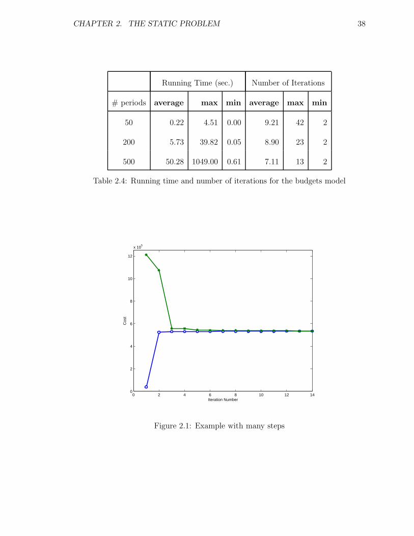
CHAPTER 2. THE STATIC PROBLEM 38
Running Time (sec.) Number of Iterations
# periods average max min average max min
50 0.22 4.51 0.00 9.21 42 2
200 5.73 39.82 0.05 8.90 23 2
500 50.28 1049.00 0.61 7.11 13 2
Table 2.4: Running time and number of iterations for the budgets model
0 2 4 6 8 10 12 140
2
4
6
8
10
12
x 105
Iteration Number
Cos
t
Figure 2.1: Example with many steps
CHAPTER 3. THE BASESTOCK PROBLEM 39
Chapter 3
The Basestock Problem
The main focus of this chapter concerns how to pick optimal basestock policies in a
robust setting, under various demand uncertainty sets D. Our focus is motivated,
primarily, by the fact that basestock policies have acquired very wide use. Basestock
policies can be shown to be optimal under many inventory models [Z00]. Further,
even though such policies may not always be optimal, they are viewed as producing
easily implementable policies in the broader context of a “real-world” supply chain,
where it is necessary to deal with a number of complex details (such as the logis-
tics of relationships with clients and suppliers) not easily handled by a mathematical
optimization engine. In the concrete example of the problem faced by our indus-
trial partner, we stress that using a (constant) basestock policy was an operational
constraint.
The inventory problem in the robust setting, using a constant (time-independent)
CHAPTER 3. THE BASESTOCK PROBLEM 40
basestock, can be described as follows:
minσ≥0
V (σ) (3.1)
where for σ ≥ 0,
V (σ) = maxd,x,u
T∑
t=1
( ctut + max htxt+1 , −btxt+1 ) (3.2)
s.t.
ut = maxσ − xt , 0, 1 ≤ t ≤ T, (3.3)
xt+1 = xt + ut − dt, 1 ≤ t ≤ T, (3.4)
(d1, d2, . . . , dT ) ∈ D. (3.5)
Here, (3.2)-(3.5) is the adversarial problem – once the demand variables (d1, d2, . . . , dT )
∈ D have been chosen, constraints (3.3)-(3.4) uniquely determine all other variables.
Note that the quantity x1 (the initial inventory level) is an input. Also, because of
the “max” in (3.2) and (3.3), the adversarial problem is non-convex.
Note that we assume σ ≥ 0 in (3.1) – in fact, our algorithms do not require
this assumption. Under special conditions, the optimal basestock might be negative;
however, we expect that the nonnegativity assumption would be commonly used and
hence we state it explicitly.
Problem (3.1) posits a constant basestock over the entire planning horizon. How-
ever, we would expect that in practice the policy would be periodically reviewed ((3.1)
CHAPTER 3. THE BASESTOCK PROBLEM 41
would be re-optimized) to adjust the basestock in a rolling horizon fashion, though
perhaps not at every time period. The stipulation for a constant basestock in (3.1)
can be viewed as an operational feature aimed at achieving stability (and “imple-
mentability”) of the policy used to operate the supply chain in the face of large, and
difficult to quantify, demand uncertainty. Clearly such a policy could prove subopti-
mal. However, when used under periodic review, and with an appropriate discounting
function and termination conditions, the policy should still prove sufficiently flexible.
In the case of our industrial partner, the use of a constant basestock level was a
required feature.
At the other extreme one could ask for a time-dependent basestock policy, i.e. we
might have a different basestock value σt for each 1 ≤ t ≤ T . We will give a result
regarding the adversarial problem in this general setting in Section 3.6. Also, there are
intermediate models between the two extremes of using different basestocks at each
time interval and a constant basestock: for example,we might allow the basestock to
change at the midpoint of the planning horizon. Or, with seasonal data, we might
use a fixed basestock value for each “season”. Even though we do not study such
models in this paper, simple extensions of the algorithms we present can in principle
handle them.
A different model is that of safety stocks. A safety stock policy with margin λ is
one that uses, at time t a basestock policy with σt = µt + λδt, where µt and δt, are
given constants (typically, estimates of the mean demand and standard deviation of
CHAPTER 3. THE BASESTOCK PROBLEM 42
demand at time t, but not necessarily so, and in our study, arbitrary constants). We
present some results concerning this model in Section 3.6.2.
The following three sections consider how to solve problem (3.1) using our generic
algorithm (1.2.1), under the risk budgets and bursty demand uncertainty models.
Section 3.2 considers the decision maker’s problem. The adversarial problem is studied
in Section 3.3 (for the risk budgets model) and Section 3.4 (bursty demands model).
3.1 Preliminaries
In the context of algorithm (1.2.1), a policy π consists of a basestock value σ, and this
will be the output of each decision maker’s problem; the corresponding adversarial
problem will consist of computing the quantity V (σ) defined in equations (1.2)-(3.3).
Prior to describing our algorithms, we note a simple observation.
Definition 3.1.1 Let d be a demand vector. For 1 ≤ t ≤ T , write Rt,d = x1 −
∑t−1j=1 dj. Write R0,d = +∞.
Definition 3.1.2 Consider a demand vector d and a basestock value σ. We denote
by t∗ = t∗σ,d the smallest t ≤ T with Rt,d ≤ σ. If no such t exists we set t∗σ,d = T + 1.
In other words, Rt,d is the amount of inventory at the start of period t if no orders
are placed in periods 1, . . . , t− 1, and t∗σ,d indicates the first period where, under the
policy using basestock σ, the starting inventory does not exceed σ.
CHAPTER 3. THE BASESTOCK PROBLEM 43
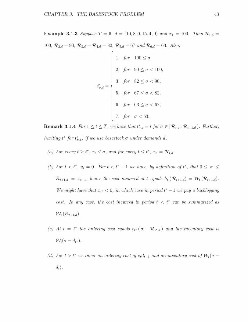
Example 3.1.3 Suppose T = 6, d = (10, 8, 0, 15, 4, 9) and x1 = 100. Then R1,d =
100, R2,d = 90, R3,d = R4,d = 82, R5,d = 67 and R6,d = 63. Also,
t∗σ,d =
1, for 100 ≤ σ,
2, for 90 ≤ σ < 100,
3, for 82 ≤ σ < 90,
5, for 67 ≤ σ < 82,
6, for 63 ≤ σ < 67,
7, for σ < 63.
Remark 3.1.4 For 1 ≤ t ≤ T , we have that t∗σ,d = t for σ ∈ [Rt,d , Rt−1,d ). Further,
(writing t∗ for t∗σ,d) if we use basestock σ under demands d,
(a) For every t ≥ t∗, xt ≤ σ, and for every t ≤ t∗, xt = Rt,d.
(b) For t < t∗, ut = 0. For t < t∗ − 1 we have, by definition of t∗, that 0 ≤ σ ≤
Rt+1,d = xt+1, hence the cost incurred at t equals ht (Rt+1,d) = Wt (Rt+1,d).
We might have that xt∗ < 0, in which case in period t∗− 1 we pay a backlogging
cost. In any case, the cost incurred in period t < t∗ can be summarized as
Wt (Rt+1,d).
(c) At t = t∗ the ordering cost equals ct∗ ( σ −Rt∗,d ) and the inventory cost is
Wt(σ − dt∗).
(d) For t > t∗ we incur an ordering cost of ctdt−1 and an inventory cost of Wt(σ −
dt).
CHAPTER 3. THE BASESTOCK PROBLEM 44
3.2 The decision maker’s problem
Here we have a finite set D ⊆ D and we wish to compute the basestock value that
minimizes the maximum cost over any demand pattern in D. Consider any demand
d ∈ D. Let icostt(σ, d) and ocostt(σ, d) denote the inventory and ordering costs
incurred at time t, under demands d, if we use basestock σ, respectively. Further, we
denote cost(σ, d) =∑
t(ocostt(σ, d) + icostt(σ, d)).
Lemma 3.2.1 For fixed d,∑
t ocostt(σ, d) is a piecewise linear function of σ with
T + 1 pieces.
Proof. Notice that
∑
t
ocostt(σ, d) =
0 if σ ≤ RT,d
ct(σ −RT,d) if RT−1,d < σ ≤ RT,d
ct(σ −Rt,d) +∑T−1
i=t ci+1di if Rt,d < σ ≤ Rt−1,d for 1 ≤ t ≤ T − 1
Here we assume that R0,d =∞ ∀d ∈ D.
Lemma 3.2.2∑
t icostt(σ, d) is a convex function of σ if either Rt,d ≥ 0 for every
1 ≤ t ≤ T + 1 or Rt,d ≤ 0 for every 1 ≤ t ≤ T + 1.
Proof. Suppose that Ri,d ≥ 0 for all 1 ≤ i ≤ T . Then the cost corresponding to
period t can be written as
CHAPTER 3. THE BASESTOCK PROBLEM 45
icostt(σ, d) =
ht(Rt,d − dt) if σ ≤ Rt,d
ht(σ − dt) if σ > Rt,d
= ht maxσ − dt,Rt,d − dt
which is a convex function of σ. Similarly if Ri,d ≤ 0 for all 1 ≤ i ≤ T , then for
1 ≤ i ≤ T
icostt(σ, d) = maxht(σ − dt),−bt(σ − dt)
which is convex in σ.
Consequently, icostt(σ, d) is a convex for all 1 ≤ t ≤ T .
Now suppose that there exist a time period 2 ≤ t′ ≤ T such that Rt′,d < 0 and
Rt′−1,d ≥ 0.
Lemma 3.2.3 cost(σ, d) is a convex function of σ for the sets L = σ : σ ≤ Rt′−1,d
and R = σ : σ ≥ Rt′−1,d.
Proof. First we consider L. For σ ∈ L the one period cost functions can be written
as follows. For 1 ≤ t ≤ t′ − 1 we have
icostt(σ, d) = ht(Rt,d − dt)
which is a linear function.
For t′ ≤ t ≤ T
icostt(σ, d) = maxht(σ − dt),−bt(σ − dt).
CHAPTER 3. THE BASESTOCK PROBLEM 46
Therefore, cost(σ, d) is convex in L.
Now we consider σ ∈ R. Similar to L we will show that one period cost is a convex
function of σ for each time period. For 1 ≤ t ≤ t′ − 1
icostt(σ, d) =
ht(Rt,d − dt) if σ ≤ Rt,d
ht(σ − dt) ifσ > Rt,d
= maxht(σ − dt), ht(Rt,d − dt).
For t′ ≤ t ≤ T
icostt(σ, d) = maxht(σ − dt),−bt(σ − dt).
icostt(σ, d) is clearly convex for all 1 ≤ t ≤ T in both cases.
Corollary 3.2.4 maxd∈D cost(σ, d) is piecewise convex with at most (T+2)|D| pieces,
with each convex piece being piecewise-linear.
Our objective is to compute σ ≥ 0 so as to minimize maxd∈D cost(σ, d). To do this,
we rely on Corollary 3.2.4 :
(i) Compute, and sort, the set of breakpoints of all functions cost(σ, d). Let 0 ≤
β1 < β2 . . . < βn be the sorted list of nonnegative breakpoints, where n ≤
(T + 2)|D|.
(ii) In each interval I of the form [0, β1], [βi, βi+1] (1 ≤ i < n) and [βn, +∞),
we have that maxd∈D cost(σ, d) is the maximum of a set of convex functions,
CHAPTER 3. THE BASESTOCK PROBLEM 47
and hence convex (in fact: piecewise linear). Let σI ∈ I be the minimizer of
maxd∈D cost(σ, d) in I.
(iii) Let I = argminI maxd∈D cost(σI , d). We set σ = σI .
In order to carry out Step (ii), in our implementation we used binary search. There
exist other algorithms that in theory, are more efficient [NW99], but empirically
our implementation proves adequate. Note that in order to carry out the binary
search in some interval I, we do not explicitly need to construct the representation
of maxd∈D cost(σ, d), restricted to I. Rather, when evaluating some σ ∈ I we simply
compute its functional value as the maximum, over d ∈ D, of cost(σ, d); and this can
done using the representation of each cost(σ, d) function.
Further, in the context of our generic algorithm 1.2.1, Step (i) can be performed
incrementally. That is to say, when adding a new demand d to D, we compute the
breakpoints of cost(σ, d) and merge these into the existing sorted list, which can be
done in linear time.
In summary, all the key steps of our algorithm for the decision maker’s problem
run linearly in T and D.
We stress that the above algorithm is independent of the underlying uncertainty
set D. In what follows, we will describe our algorithms for the adversarial problem,
under the risk budgets and bursty demand uncertainty models.
CHAPTER 3. THE BASESTOCK PROBLEM 48
3.3 The adversarial problem under the risk bud-
gets model
In this section we consider the adversarial model under the demand uncertainty set
D given by (2.3)-(2.5), assuming that a fixed basestock σ has been given. We let
(d∗, z∗) denote the optimal demand (and risks) vector chosen by the adversary. We
first want to characterize structural properties of (d∗, z∗). In what follows, we write
t∗ for t∗σ,d∗ . First we have the following easy result:
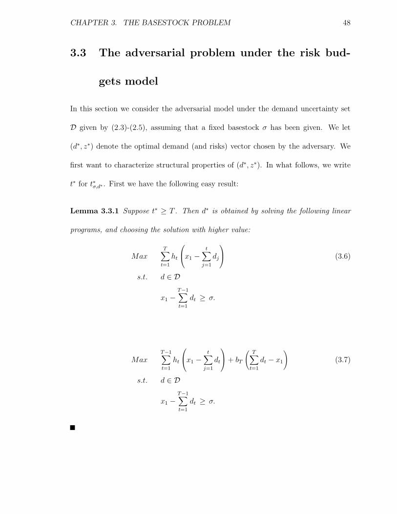
Lemma 3.3.1 Suppose t∗ ≥ T . Then d∗ is obtained by solving the following linear
programs, and choosing the solution with higher value:
MaxT∑
t=1
ht
x1 −t∑
j=1
dj
(3.6)
s.t. d ∈ D
x1 −T−1∑
t=1
dt ≥ σ.
MaxT−1∑
t=1
ht
x1 −t∑
j=1
dt
+ bT
(
T∑
t=1
dt − x1
)
(3.7)
s.t. d ∈ D
x1 −T−1∑
t=1
dt ≥ σ.
CHAPTER 3. THE BASESTOCK PROBLEM 49
Lemma 3.3.1 provides one case for our adversarial algorithm. In what follows we
will assume that t∗ < T and describe algorithms for this case. We will describe two
algorithms: an exact algorithm, which solves the problem to proved optimality, and a
much faster approximate algorithm which does not prove optimality but nevertheless
produces a “strong” demand pattern d which, in the language of our generic algorithm
(1.2.1), quickly improves on the working set D. The exact algorithm requires (in a
conservative worst-case estimate) the solution of up to O(T 4 ΓT ) warm-started linear
programs with fewer than 4T variables; as we show in Section 3.5 it nevertheless can
be implemented to run quite efficiently. The approximate algorithm, on the other
hand, is significantly faster.
Some additional remarks on the exact algorithm:
(a) When the Γt are integral, the step count reduces to O(T 2 ΓT ). In addition, if
Γt = t for each t (i.e. the uncertainty set reduces to the intervals [µt−δt, µt+δt])
the complexity reduces to O(T 2), with no linear programs solved. See Section
3.3.6 for details.
(b) The case of integral Γt is of interest because if we use the uncertainty set with
risk budgets Γft = bΓtc we obtain a lower bound on the min-max problem,
whereas if we use then risk budgets Γct = dΓte we obtain an upper bound. In
fact, the superposition of the two uncertainty sets should provide a good ap-
proximation to the min-max problem (see Section 3.6.4). Further,we present a
CHAPTER 3. THE BASESTOCK PROBLEM 50
bounding procedure based on this idea, which proves excellent bounds, signifi-
cantly faster than the algorithm for fractional Γt.
We begin with the exact algorithm. Lemmas 3.3.2 and 3.3.3 and Remark 3.3.4,
all given below, provide some structural properties of an optimal solution to the
adversarial problem. Sections 3.3.1, 3.3.2 and 3.3.3 describe the technical details of
our approach. The overall algorithm is put together in Section 3.3.4. The approximate
algorithm is described in Section 3.3.5, the case with the integral budgets is considered
in Section 3.3.6 and the bounding procedure based on integral budgets is given in
Section 3.3.7.
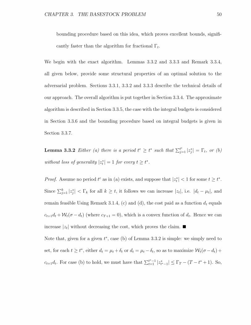
Lemma 3.3.2 Either (a) there is a period te ≥ t∗ such that∑te
j=1 |z∗j | = Γt, or (b)
without loss of generality |z∗t | = 1 for every t ≥ t∗.
Proof. Assume no period te as in (a) exists, and suppose that |z∗t | < 1 for some t ≥ t∗.
Since∑k
j=1 |z∗j | < Γk for all k ≥ t, it follows we can increase |zt|, i.e. |dt − µt|, and
remain feasible Using Remark 3.1.4, (c) and (d), the cost paid as a function dt equals
ct+1dt +Wt(σ− dt) (where cT+1 = 0), which is a convex function of dt. Hence we can
increase |zt| without decreasing the cost, which proves the claim.
Note that, given for a given t∗, case (b) of Lemma 3.3.2 is simple: we simply need to
set, for each t ≥ t∗, either dt = µt + δt or dt = µt− δt, so as to maximize Wt(σ− dt)+
ct+1dt. For case (b) to hold, we must have that∑t∗−1
t=1 |z∗t∗−1| ≤ ΓT − (T − t∗ + 1). So,
CHAPTER 3. THE BASESTOCK PROBLEM 51
for a given t∗, case (b) amounts to solving the linear program:
Maxt∗−1∑
t=1
ht
x1 −t∑
j=1
dt
+ ct∗
(
σ − (x1 −t∗−1∑
t=1
dt)
)
(3.8)
s.t. dt = µt + δtzt, 1 ≤ t ≤ t∗ − 1,
zt ∈ [−1, 1], 1 ≤ t ≤ t∗ − 1,
t∑
j=1
|zj| ≤ Γt, 1 ≤ t ≤ t∗ − 2,
t∗−1∑
j=1
|zt∗−1| ≤ ΓT − (T − t∗ + 1),
x1 −t∗−2∑
t=1
dt ≥ σ,
x1 −t∗−1∑
t=1
dt ≤ σ.
In total, case (b) amounts to T linear programs of type (3.8). In what follows, we
assume that case (a) holds, and that furthermore the period te is chosen as small as
possible.
Lemma 3.3.3 Without loss of generality, there is at most one period tf with t∗ ≤
tf ≤ te, such that 0 < |z∗tf | < 1.
Proof. If we have t∗ = te the result is clear, and if t∗ < te the result follows because
the cost incurred in periods t∗, . . . , te is a convex function of the demands in those
periods.
CHAPTER 3. THE BASESTOCK PROBLEM 52
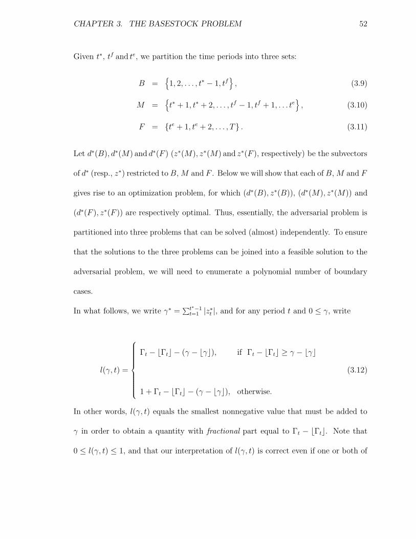
Given t∗, tf and te, we partition the time periods into three sets:
B =
1, 2, . . . , t∗ − 1, tf
, (3.9)
M =
t∗ + 1, t∗ + 2, . . . , tf − 1, tf + 1, . . . te
, (3.10)
F = te + 1, te + 2, . . . , T . (3.11)
Let d∗(B), d∗(M) and d∗(F ) (z∗(M), z∗(M) and z∗(F ), respectively) be the subvectors
of d∗ (resp., z∗) restricted to B, M and F . Below we will show that each of B, M and F
gives rise to an optimization problem, for which (d∗(B), z∗(B)), (d∗(M), z∗(M)) and
(d∗(F ), z∗(F )) are respectively optimal. Thus, essentially, the adversarial problem is
partitioned into three problems that can be solved (almost) independently. To ensure
that the solutions to the three problems can be joined into a feasible solution to the
adversarial problem, we will need to enumerate a polynomial number of boundary
cases.
In what follows, we write γ∗ =∑t∗−1
t=1 |z∗t |, and for any period t and 0 ≤ γ, write
l(γ, t) =
Γt − bΓtc − (γ − bγc), if Γt − bΓtc ≥ γ − bγc
1 + Γt − bΓtc − (γ − bγc), otherwise.
(3.12)
In other words, l(γ, t) equals the smallest nonnegative value that must be added to
γ in order to obtain a quantity with fractional part equal to Γt − bΓtc. Note that
0 ≤ l(γ, t) ≤ 1, and that our interpretation of l(γ, t) is correct even if one or both of
CHAPTER 3. THE BASESTOCK PROBLEM 53
Γt and γ are integral.
Remark 3.3.4 |z∗tf | = l(γ∗, te).
In the following sections 3.3.1, 3.3.2, 3.3.3 we we describe optimization problems
arising from M , B and F that are solved by (d∗(M), z∗(M)), (d∗(B), z∗(B)), and
(d∗(F ), z∗(F )), respectively, assuming that there is a period tf as in Lemma 3.3.3.
3.3.1 Handling M.
We consider first
PM(γ, t∗, tf , te) :
maxd,z
∑
i∈M
(Wi(σ − di) + ci+1di)
s.t.
di = µi + δizi ∀i ∈M (3.13)
i∑
j=t∗|zi| ≤ bΓi − γc t∗ ≤ i ≤ tf − 1 (3.14)
tf−1∑
j=t∗|zi| ≤ bΓtf − (γ + l(γ, te))c (3.15)
tf−1∑
j=t∗|zi| +
i∑
j=tf+1
|zi| ≤ bΓi − (γ + l(γ, te))c, tf + 1 ≤ i ≤ te, (3.16)
−1 ≤ zi ≤ 1 ∀i ∈M,
Lemma 3.3.5 (d∗(M), z∗(M)) is an optimal solution to PM(γ∗, t∗, tf , te).
CHAPTER 3. THE BASESTOCK PROBLEM 54
Proof. First, (d∗(M), z∗(M)) is feasible for this problem. This follows by Remark
3.3.4 because in periods i ∈ M we have∑i
j=t∗ |z∗i | ≤ Γi − γ∗, and furthermore the
|z∗i | are integral (0 or 1) by definition of M . Conversely, if (d(M), z(M)) is optimal
solution to PM(γ∗, t∗, tf , te), then (d∗(B), d(M), d∗(F )) is a feasible solution to the
adversarial problem, and the result follows.
Note that PM(γ, t∗, tf , te) can be formulated as a mixed-integer program, much
like (2.38). A subject for research would be to study under what conditions the linear
programming relaxation of the formulation has an integral solution.
Later we will show how to solve PM(γ, t∗, tf , te) in polynomial time. First, note
that the right-hand sides of constraints (3.15) and (3.16) depend on bγc, and not γ.
Further, suppose we write ft = Γt−bΓtc for t ∈ t∗, t∗ + 1, . . . , tf − 1∪ te, and let
f(1), f(2), . . . , f(tf−t∗+1) be the sorted values ft. Also write f(0) = 0 and f(tt−t∗+2) = 1.
Thus, if we fix bγc, and fix some i, 0 ≤ i ≤ tf − t∗, then any two values γ with
f(i) < γ − bγc ≤ f(i+1) will produce the same right-hand sides for constraints (3.14)-
(3.16). Thus, for fixed bγc, t∗, tf , and te there are only O(tf − t∗) distinct problems
PM(γ, t∗, tf , te).
3.3.2 Handling B.
Next we turn to set B (c.f. (3.9)). Consider the optimization problem, for 0 ≤ k ≤
Γt∗−1 and 0 ≤ j ≤ tf − t∗ + 1:
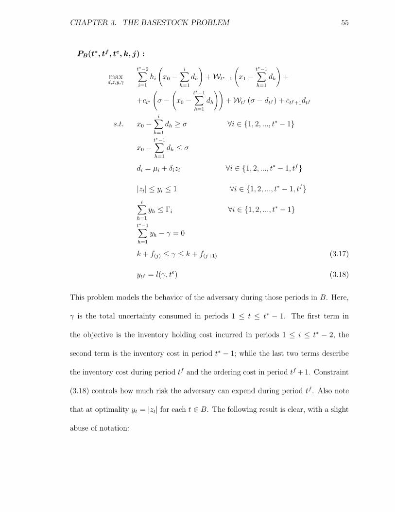
CHAPTER 3. THE BASESTOCK PROBLEM 55
PB(t∗, tf , te, k, j) :
maxd,z,y,γ
t∗−2∑
i=1
hi
(
x0 −i∑
h=1
dh
)
+Wt∗−1
(
x1 −t∗−1∑
h=1
dh
)
+
+ct∗
(
σ −
(
x0 −t∗−1∑
h=1
dh
))
+Wtf (σ − dtf ) + ctf+1dtf
s.t. x0 −i∑
h=1
dh ≥ σ ∀i ∈ 1, 2, ..., t∗ − 1
x0 −t∗−1∑
h=1
dh ≤ σ
di = µi + δizi ∀i ∈ 1, 2, ..., t∗ − 1, tf
|zi| ≤ yi ≤ 1 ∀i ∈ 1, 2, ..., t∗ − 1, tf
i∑
h=1
yh ≤ Γi ∀i ∈ 1, 2, ..., t∗ − 1
t∗−1∑
h=1
yh − γ = 0
k + f(j) ≤ γ ≤ k + f(j+1) (3.17)
ytf = l(γ, te) (3.18)
This problem models the behavior of the adversary during those periods in B. Here,
γ is the total uncertainty consumed in periods 1 ≤ t ≤ t∗ − 1. The first term in
the objective is the inventory holding cost incurred in periods 1 ≤ i ≤ t∗ − 2, the
second term is the inventory cost in period t∗ − 1; while the last two terms describe
the inventory cost during period tf and the ordering cost in period tf +1. Constraint
(3.18) controls how much risk the adversary can expend during period tf . Also note
that at optimality yt = |zt| for each t ∈ B. The following result is clear, with a slight
abuse of notation:
CHAPTER 3. THE BASESTOCK PROBLEM 56
Lemma 3.3.6 Suppose that k + f(j) ≤ γ∗ ≤ k + f(j+1) for integers 0 ≤ k ≤ bΓt∗−1c
and 1 ≤ j ≤ tf − t∗ + 2. Then, (d∗(B), z∗(B), γ∗) solves PB(t∗, tf , te, k, j).
Next, we show how to replace PB(t∗, tf , te, k, j) with at most four linear programs.
First, since the objective of PB(t∗, tf , te, k, j) contains just two functions Wt, we can
reduce the problem to at most four problems, each with a linear objective function
and with the same constraints as PB(t∗, tf , te, k, j). There remains the expression
l(γ, te) in the right-hand side of (3.18). We handle this as follows:
(i) Suppose f(j) 6= fte , and f(j+1) < 1. Then, for every γ ∈ [k + f(j), k + f(j+1)], we
have that in the definition of l(γ, te) (see eq. (3.12)) the same case will always
apply; and furthermore γ − bγc = γ − k. We conclude that l(γ, te) is linear in
γ.
(ii) Suppose now that j is such that f(j) = fte and f(j+1) < 1. Then we replace
(3.18) with the constraint
ytf = 1 + fte − (γ − k). (3.19)
The right-hand side of (3.19) differs from l(γ, te) only at γ = k + fte where
it equals 1, whereas l(k + fte , te) = 0. Denote the new optimization problem
LB(t∗, tf , te, k, j). We claim that (d∗(B), z∗(B), γ∗) solves LB(t∗, tf , te, k, j).
If not, in every optimal solution we must have k + f(j) = γ and k + f(j) < γ∗.
Consequently, since the right-hand side of (3.19) is linear, then for ε > 0 small
CHAPTER 3. THE BASESTOCK PROBLEM 57
enough we can find a feasible solution to LB(t∗, tf , te, k, j) with γ = k + f(j) + ε
and with optimality error O(ε). Such a solution would be strictly better than
(d∗(B), z∗(B), γ∗) if ε is small enough; furthermore such a solution would be
feasible for PB(t∗, tf , te, k, j), contradicting Lemma 3.3.6.
As a final note for this case, suppose k+fte < γ∗, and that we solve LB(t∗, tf , te, k, j)
and obtain an optimal solution (d, z, γ) with γ = k + fte . This is a solution to
one of the (up to) four linear programs corresponding to LB(t∗, tf , te, k, j); thus,
without loss of generality, the entire segment between (d, z, γ) and (d∗(B), z∗(B), γ∗)
is made up of optimal solutions to LB(t∗, tf , te, k, j). Hence, by performing a
parametric simplex pivot we can obtain, from (d, z, γ), an optimal solution that
has a value of γ strictly larger than k + fte .
(iii) Finally, assume now that f(j+1) = 1. Note that fte < 1, so fte ≤ f(j). In this
case we again replace (3.18) with (3.19). In this case, the substitution is correct
except when γ = k + 1 ( where l(k + 1, te) = fte , whereas the right-hand side
of (3.19) equals 1 + fte) and, if fte = f(j) at γ = k + f(j). Note that γ∗ < k + 1
(since otherwise z∗tf would be integral). An argument similar to that in case (ii)
shows, again, that (d∗(B), z∗(B)) solves LB(t∗, tf , te, k, j).
The above observations are summarized as follows:
Lemma 3.3.7 Problem PB(t∗, tf , te, k, j) is solved by (d∗(B), z∗(B), γ∗) and it re-
duces to at most four linear programs.
CHAPTER 3. THE BASESTOCK PROBLEM 58
3.3.3 Handling F
Finally, we consider the set F of time periods. For t < T , define
PF (t) :
maxT∑
i=t
Wi(σ − di) +T+1∑
i=t+1
cidi−1 (3.20)
s.t. di = µi + δizi t ≤ i ≤ T
i∑
j=t+1
|zi| ≤ Γi − Γt−1 t ≤ i ≤ T
−1 ≤ zi ≤ 1 t ≤ i ≤ T
The following is clear:
Lemma 3.3.8 If te < T , (d∗(F ), z∗(F )) solves PF (te + 1).
3.3.4 The algorithm
Assuming first that there is a time period tf as in Lemma 3.3.3, our algorithm ex-
amines every 5-tuple (t∗, tf , te, k, j), where 1 ≤ t∗ ≤ tf ≤ te ≤ T , 0 ≤ k ≤ Γt∗−1
and 0 ≤ j ≤ tf − t∗ + 1. For each such 5-tuple, we solve the three problems
PB(t∗, tf , te, k, j), PM(γ, t∗, tf , te) (where we pick any γ with k +f(j) < γ < k +f(j+1))
and PF (te + 1). By Lemmas 3.3.7, 3.3.6 and 3.3.8 (also see the remarks preceding
Lemma 3.3.7), the solutions to at least one such triple of problems can be assembled
into an optimal solution to the adversarial problem.
The case where there is no time period tf as in Lemma 3.3.3 is handled in a similar

CHAPTER 3. THE BASESTOCK PROBLEM 59
way: here we amend problem PB by removing the last two terms in the objective,
and we amend problem PM by removing constraints (3.15) and suitably modifying
constraint (3.16).
In order to complete the description of the algorithm, we need to explain how to
solve each problem PM and PF (we have already shown that the PB reduce to linear
programs).
A problem PM(γ, t∗, tf , te) can be solved using dynamic programming, with a stage
for each time period t between t∗ and te, and a state corresponding to the risk budget
consumed by period t. Rather than solving each problem separately, we can embed
them into a smaller number of families. For example, given γ and tf then the stages
and states corresponding to periods between tf and te are independent of t∗, and the
value of a state depends only on te. Further improvements are possible (see Appendix
A). The procedure as described requires O(T 4 ΓT ) steps.
Next, consider a problem of type PF (t). Clearly, this is just the adversarial prob-
lem restricted to periods t ≤ i ≤ T , using the risk budgets Γi−Γt−1, and with starting
inventory σ. Notice that this last condition implies that t∗ = t. Consequently, PF (t)
reduces to a set of trivial (one period) problems PB, and problems of type PM . Hence,
the up-front solution of all problems PM as described in the previous paragraph can
be used to quickly solve each problem PF (t).
Finally, a comment on the problems LB(t∗, tf , te, k, j). There is a total of O(T 4 ΓT )
such problems, and as discussed above, each such problem reduces to up to four
CHAPTER 3. THE BASESTOCK PROBLEM 60
linear programs. These linear programs should be warm-started, i.e. not solved
from scratch. For example, parameter j only affects constraint (3.17); re-optimizing
starting from the solution to the problem corresponding to j + 1 (and all other pa-
rameters identical) will typically require a tiny number of pivots. Similarly with
t∗, tf , te, and k. This detail, together with other implementations tricks, is impor-
tant.
3.3.5 The approximate adversarial algorithm
In the discussion above we focused on solving the adversarial problem in Algorithm
1.2.1 exactly. Even though our algorithm runs in polynomial time, it is very conser-
vative: it examines demand patterns that are unlikely to prove optimal except under
extreme data conditions.
Thus, it is appealing to use a possibly suboptimal algorithm. The benefit of
this would be that we would have much faster iterations, while, if the suboptimal
algorithm were “smart” enough, we would still reap the benefit of updating the set
D in Algorithm 1.2.1 with demand patterns that fairly accurately approximate what
the adversary can do. Of course, if we follow this approach, the quantity U computed
in Step 2 of Algorithm 1.2.1 no longer qualifies as an upper bound to the min-max
problem, though L certainly is a lower bound.
Hence, we can use the following approach: run Algorithm 1.2.1 as stated in its
CHAPTER 3. THE BASESTOCK PROBLEM 61
description, but using a suboptimal algorithm to handle the adversarial problem.
Whenever U − L is small, we run the exact adversarial algorithm, at which point
the value of the adversarial problem does become a valid upper bound. This might
allow us to terminate immediately if the gap is small. If not, we continue with the
generic algorithm, once again using the suboptimal procedure to solve the adversarial
problem. In theory, the exact algorithm should be run, for example, every k iterations
for some k, but in our experience this was not needed.
The particular suboptimal algorithm we used was based on a simple idea. Our ap-
proach for the exact algorithm solved problems PM(γ, t∗, tf , te) and PB(t∗, tf , te, k, j)
for all appropriate 5-tuples (t∗, tf , te, k, j). In the suboptimal algorithm, instead, given
t∗ and te we compute a particular period to serve as tf . Recall (Remark 3.3.4) that
the risk consumption at tf should equal l(γ, te). Further, at period tf inventory is
already at or below basestock, and so the inventory cost at tf will equalWtf (σ−dtf );
by applying this formula with
dtf = µtf ± l(γ, te) δtf (3.21)
we compute the inventory cost at tf , assuming tf = tf . On the other hand, if tf 6= tf ,
the maximum inventory cost at tf will be attained by
dtf = µtf ± δtf . (3.22)
Our method picks that period tf for which the decrease from (3.22) to (3.21) is
minimum. Notice that by doing so we ignore the relation between the period tf and

CHAPTER 3. THE BASESTOCK PROBLEM 62
problem PB(t∗, tf , te, k, j). However, the impact on optimality should be small. As
we will see, this approximation dramatically speeds up the algorithm.
3.3.6 Integral budgets case
When we have integral budgets the problem becomes easier. We can eliminate some
of the components in the 5-tuple (t∗, tf , te, k, j) that we examine in our original algo-
rithm. First of all, we do not need last component, since it is only used to keep track
of the fractional parts of the budgets. Moreover, the following Lemma shows that we
can also eliminate te.
Lemma 3.3.9 z∗t is integral for all te ≤ t ≤ T .
Proof. Suppose that the Lemma is not true and there exist a time period after te that
has fractional risk consumption. Let t1 be the smallest of such periods. Then, there
exists another time period t2 > t1 whose risk consumption is fractional: otherwise,
we can reduce the risk consumption at t1 to zero, without decreasing cost; or we can
increase it (without exceeding budgets) and increase cost. However due to convexity
of the cost we can either increase the risk in t1 and decrease the risk in t2 by the same
amount or do the reverse and get a new demand pattern that has a cost which is a
least as large as the former demand pattern.
Using Lemma 3.3.9, we can extend the dynamic program for computing the cost for
period t∗ ≤ t ≤ te to compute the cost for the periods te < t ≤ T and we can eliminate
CHAPTER 3. THE BASESTOCK PROBLEM 63
te. Therefore, instead of solving PB, PM and PF for each possible value of the 5-tuple
(t∗, tf , te, k, j), we solve PB for each possible value of triple (t∗, tf , k) (we change r.h.s.
of 3.18 with 1− (γ−bγc)) and we use the extended dynamic program to compute the
cost for periods t∗, t∗ +1, . . . , T for each value of (t∗, tf , k). Consequently, the number
of steps is reduced to O(T 2ΓT ) for the integral budgets case.
When Γt = t for each t, we can further decrease the complexity of the algorithm.
In this case, since the risk budgets have no impact, we can eliminate the fourth
component of our 5-tuples (the integral part of the risk budget that is consumed up
to time period t∗). Therefore, the step count further reduces to O(T 2).
3.3.7 A bounding procedure for the risk budgets model
A simple observation is that the exact algorithm described above runs much faster
when the Γt are integral. In the language of the previous sections, this follows from
the fact that if the Γt are integral, then we must have tf = te. This observation
motivates the following approach:
1. Run the algorithm using risk budgets dΓte. The value of this problem is an
upper bound on the min-max problem with the original Γt (e.g., the adversary
is more powerful).
2. Run the algorithm using risk budgets bΓtc. The value of this problem is a lower
bound on the min-max problem with the original Γt, and the demand patterns
CHAPTER 3. THE BASESTOCK PROBLEM 64
produced by the adversary are valid.
In our testing, this scheme proved extremely effective, producing very tight bounds
quite quickly. Clearly, we might obtain poor quality bounds in cases where T is small
– but then the exact algorithm will be fast enough.
We integrate this procedure into the overall algorithm as follows. Consider the
first instance where we would run the exact algorithm as indicated in Section 3.3.5
(e.g. when the lower bound L and the quantity U are close). Then, we run the
bounding procedure instead of the exact algorithm. Optionally, if the upper bound
proved by the procedure is close to the current lower bound, we can terminate.
3.4 The adversarial problem under the bursty de-
mand model
For the reader’s convenience, we restate the bursty demand model. Here, period t is
either normal, meaning dt ∈ [µt−δt, µt+δt] (where 0 ≤ δt ≤ µt are given parameters),
or it is exceptional, meaning dt = Pt, where Pt is a given parameter. Further, in any
set of W consecutive periods there is at most one exceptional period.
From a purely theoretical standpoint, we have the following result:
Theorem 3.4.1 The adversarial problem in the bursty demand model is NP-hard.
Proof. See Section B.1.
CHAPTER 3. THE BASESTOCK PROBLEM 65
This result is possibly of theoretical interest only, because it is not clear just how
large T would be in a practical application. Nevertheless, the result does highlight
that, most likely, a polynomial-time algorithm for the adversarial problem does not
exist.
Our approach is as follows. For any demand pattern d, define the time period t∗ as
in Section 3.1: t∗ is the earliest period such that the starting inventory is at most σ.
Then the maximum cost attainable by the adversary during periods 1 through t∗− 1,
plus the order cost at period t∗, assuming that the last exceptional period is t∗ − k
(k = 1, . . . , mint∗, W) is obtained by solving the following optimization problem:
IP (t∗, k) :
maxt∗−2∑
i=1
hi
x1 −i∑
j=1
dj
+Wt∗−1
x1 −t∗−1∑
j=1
dj
+ ct∗(σ − (x1 −t∗−1∑
j=1
dj))
s.t. x1 −t∑
j=1
dj ≥ σ 1 ≤ t ≤ t∗ − 2 (3.23)
x1 −t∗−1∑
j=1
dj ≤ σ (3.24)
dt = st + ItPt, It ∈ 0, 1 1 ≤ t ≤ t∗ − 1 (3.25)
(1− It)(µt − δt) ≤ st ≤ (1− It)(µt + δt) 1 ≤ t ≤ t∗ − 1 (3.26)
t+W−1∑
i=t
It ≤ 1 1 ≤ t ≤ t∗ −W (3.27)
It∗−k = 1 (3.28)
In this formulation, the 0−1 variable It is used to indicate exceptional periods. If
we set k = 0, and replace (3.28) with the constraints It = 0 for t = 1, . . . , mint∗, W,
CHAPTER 3. THE BASESTOCK PROBLEM 66
then we obtain the maximum cost attainable by the adversary assuming that there
is no exceptional period among the last W periods.
We will return to problem IP (t∗, k) below, but first we consider the periods after
t∗. This part can be handled with a simple dynamic programming recursion. For
t = t∗, . . . , T and k = 0, 1, . . . , mint − t∗, W, let Vt(k) denote the maximum cost
attainable by the adversary in periods t, . . . , T (not counting the ordering cost at t)
assuming that the last exceptional period prior to t is period t − k (with the same
interpretation as before for k = 0). The recursion goes as follows:
For t = t∗, ..., T − 1, we have
Vt(0) = maxd∈µt−δt,µt+δt,Pt
Wt(σ − d) + ct+1d + Vt+1 (I) , (3.29)
where we set I = 1 when we choose d = Pt, and otherwise we set I = 0. For
k = 1, . . . , W − 1 and t < T ,
Vt(k) = maxd∈µt−δt,µt+δt
Wt(σ − d) + ct+1d + Vt+1(k + 1 (mod W )). (3.30)
For t = T , we set
VT (0) = maxd∈µT −δT ,µT +δT ,Pt
WT (σ − d), (3.31)
and for k = 1, ..., W − 1
VT (k) = maxd∈µT −δT ,µT +δT
WT (σ − d). (3.32)
Clearly this recursion runs in polynomial time. Further, for each t and k we can
put together a solution to IP (t, k), and the optimizer for Vt(k), to obtain a feasible
CHAPTER 3. THE BASESTOCK PROBLEM 67
solution to the adversarial problem, and the best such solution will clearly be the
optimal solution. It is clear that the Vt(k) can computed efficiently; now we return
to the mixed-integer program IP (t, k).
Consider the system made up of those constraints involving the 0− 1 variables It,
namely (3.25), (3.26) and (3.27) (we do not include (3.28) since it just fixes a variable)
plus the bounds 0 ≤ It ≤ 1 for all t. It can be shown that this system defines an
integral polyhedron (that is to say, a polyhedron each of whose extreme points has
0 − 1 values on the It variables). This essentially is a known fact; in particular
constraints (3.27) describe a vertex-packing polyhedron on an interval graph (see
[NW88] for background).
The consequence of this is that problem IP (t∗, k), or, rather, each of the two linear
objective problems obtained by considering the two cases forWt∗−1, is a mixed-integer
programming problem over an integer polyhedron plus two side constraints (which do
not involve the 0− 1 variables). We would thus expect IP (t∗, k) to be easily solvable
as a general mixed-integer program. And this proves to be exactly the case: using
commercial software, instances with T even in the hundreds, are solved in hundredths
of a second.
CHAPTER 3. THE BASESTOCK PROBLEM 68
3.5 Experiments with the basestock model
Our computational experiments are of two kinds. First, we want to study the con-
vergence properties of the algorithms. Second, we want to investigate qualitative
properties of the models studied in this paper.
3.5.1 The risk budgets model
In Table 3.1 we study the behavior of the exact algorithm and that of the bounding
procedure described in Section 3.3.7. The column headed “Cost Gap” indicates the
percentage error between the available upper and lower bounds when the early ter-
mination condition provided by the bounding procedure was tested. To produce the
statistics in the table, for each data type we ran 150 randomly generated instances
each with T = 100 time periods. Running times are in seconds. We see that, on aver-
age, the bounding procedure proves bounds with approximately a 1.7% gap. Another
point to be stressed is that in both the exact algorithm and in the early termination
version, the running time is dominated by the adversarial problem computations.
Table 3.1 may overstate the difference between the early termination solution and the
optimal solution: in Table 3.2 we compare the early termination basestock with the
optimal basestock level (same data as Table 3.1). We see that in most cases the early
termination basestock indeed provides an excellent approximation to the optimum.
Table 3.3 presents the running time of the algorithm for instances with integral
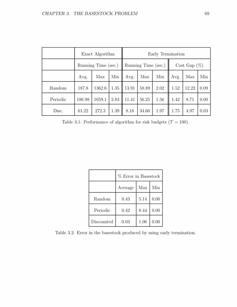
CHAPTER 3. THE BASESTOCK PROBLEM 69
Exact Algorithm Early Termination
Running Time (sec.) Running Time (sec.) Cost Gap (%)
Avg. Max Min Avg. Max Min Avg. Max Min
Random 187.8 1362.6 1.35 13.91 58.89 2.02 1.52 12.22 0.09
Periodic 186.98 1659.1 2.83 11.41 56.25 1.56 1.42 8.71 0.00
Disc. 61.22 272.3 1.39 8.18 34.60 1.97 1.75 4.97 0.03
Table 3.1: Performance of algorithm for risk budgets (T = 100).
% Error in Basestock
Average Max Min
Random 0.43 5.14 0.00
Periodic 0.42 8.44 0.00
Discounted 0.03 1.06 0.00
Table 3.2: Error in the basestock produced by using early termination.
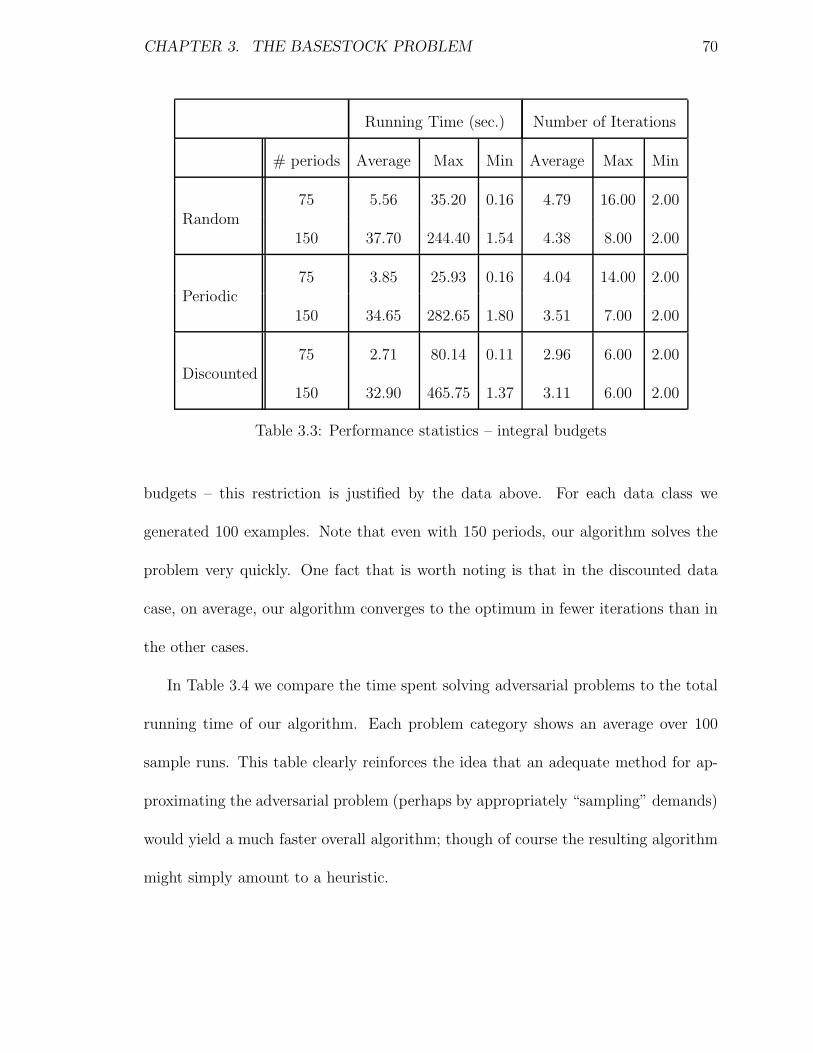
CHAPTER 3. THE BASESTOCK PROBLEM 70
Running Time (sec.) Number of Iterations
# periods Average Max Min Average Max Min
Random75 5.56 35.20 0.16 4.79 16.00 2.00
150 37.70 244.40 1.54 4.38 8.00 2.00
Periodic75 3.85 25.93 0.16 4.04 14.00 2.00
150 34.65 282.65 1.80 3.51 7.00 2.00
Discounted75 2.71 80.14 0.11 2.96 6.00 2.00
150 32.90 465.75 1.37 3.11 6.00 2.00
Table 3.3: Performance statistics – integral budgets
budgets – this restriction is justified by the data above. For each data class we
generated 100 examples. Note that even with 150 periods, our algorithm solves the
problem very quickly. One fact that is worth noting is that in the discounted data
case, on average, our algorithm converges to the optimum in fewer iterations than in
the other cases.
In Table 3.4 we compare the time spent solving adversarial problems to the total
running time of our algorithm. Each problem category shows an average over 100
sample runs. This table clearly reinforces the idea that an adequate method for ap-
proximating the adversarial problem (perhaps by appropriately “sampling” demands)
would yield a much faster overall algorithm; though of course the resulting algorithm
might simply amount to a heuristic.
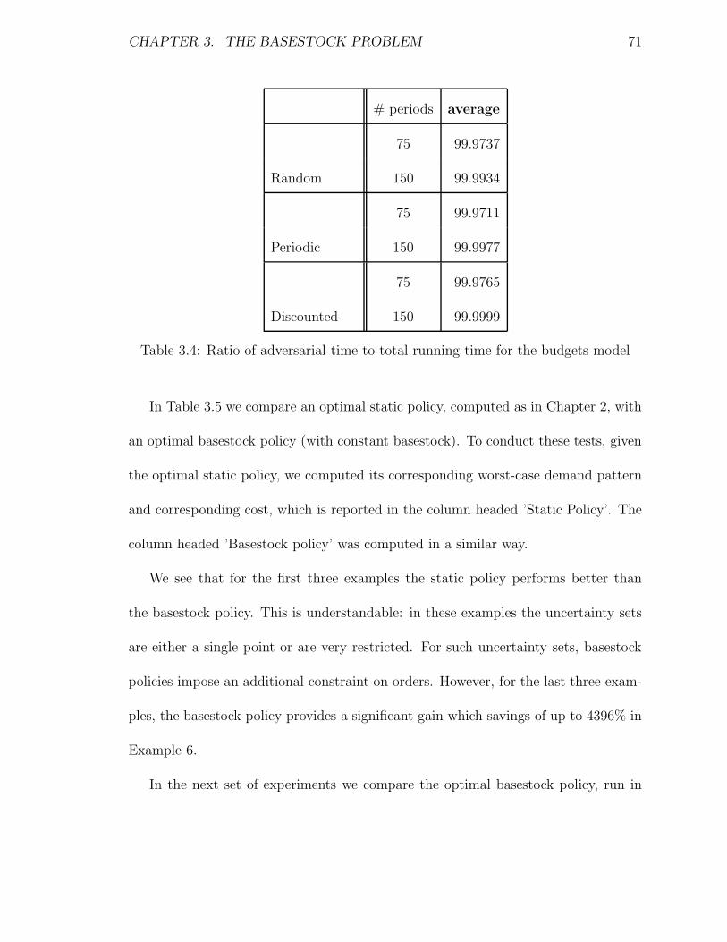
CHAPTER 3. THE BASESTOCK PROBLEM 71
# periods average
Random
75 99.9737
150 99.9934
Periodic
75 99.9711
150 99.9977
Discounted
75 99.9765
150 99.9999
Table 3.4: Ratio of adversarial time to total running time for the budgets model
In Table 3.5 we compare an optimal static policy, computed as in Chapter 2, with
an optimal basestock policy (with constant basestock). To conduct these tests, given
the optimal static policy, we computed its corresponding worst-case demand pattern
and corresponding cost, which is reported in the column headed ’Static Policy’. The
column headed ’Basestock policy’ was computed in a similar way.
We see that for the first three examples the static policy performs better than
the basestock policy. This is understandable: in these examples the uncertainty sets
are either a single point or are very restricted. For such uncertainty sets, basestock
policies impose an additional constraint on orders. However, for the last three exam-
ples, the basestock policy provides a significant gain which savings of up to 4396% in
Example 6.
In the next set of experiments we compare the optimal basestock policy, run in
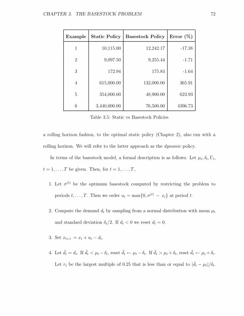
CHAPTER 3. THE BASESTOCK PROBLEM 72
Example Static Policy Basestock Policy Error (%)
1 10,115.00 12,242.17 -17.38
2 9,097.50 9,255.44 -1.71
3 172.94 175.83 -1.64
4 615,000.00 132,000.00 365.91
5 354,000.00 48,900.00 623.93
6 3,440,000.00 76,500.00 4396.73
Table 3.5: Static vs Basestock Policies
a rolling horizon fashion, to the optimal static policy (Chapter 2), also run with a
rolling horizon. We will refer to the latter approach as the dynamic policy.
In terms of the basestock model, a formal description is as follows. Let µt, δt, Γt,
t = 1, . . . , T be given. Then, for t = 1, . . . , T ,
1. Let σ(t) be the optimum basestock computed by restricting the problem to
periods t, . . . , T . Then we order ut = max0, σ(t) − xt at period t.
2. Compute the demand dt by sampling from a normal distribution with mean µt
and standard deviation δt/2. If dt < 0 we reset dt = 0.
3. Set xt+1 = xt + ut − dt.
4. Let dt = dt. If dt < µt− δt, reset dt ← µt− δt. If dt > µt + δt, reset dt ← µt + δt.
Let rt be the largest multiple of 0.25 that is less than or equal to |dt − µt|/δt.
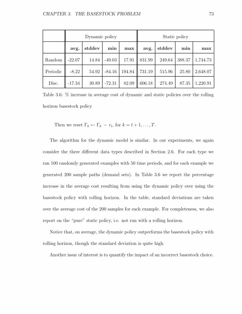
CHAPTER 3. THE BASESTOCK PROBLEM 73
Dynamic policy Static policy
avg. stddev min max avg. stddev min max
Random -22.07 14.84 -49.03 17.91 831.99 249.64 388.37 1,744.73
Periodic -8.22 54.92 -84.16 194.84 731.19 515.96 25.80 2,648.07
Disc. -17.34 30.89 -72.31 82.09 606.18 274.49 87.35 1,220.91
Table 3.6: % increase in average cost of dynamic and static policies over the rolling
horizon basestock policy
Then we reset Γk ← Γk − rt, for k = t + 1, . . . , T .
The algorithm for the dynamic model is similar. In our experiments, we again
consider the three different data types described in Section 2.6. For each type we
ran 100 randomly generated examples with 50 time periods, and for each example we
generated 200 sample paths (demand sets). In Table 3.6 we report the percentage
increase in the average cost resulting from using the dynamic policy over using the
basestock policy with rolling horizon. In the table, standard deviations are taken
over the average cost of the 200 samples for each example. For completeness, we also
report on the “pure” static policy, i.e. not run with a rolling horizon.
Notice that, on average, the dynamic policy outperforms the basestock policy with
rolling horizon, though the standard deviation is quite high.
Another issue of interest is to quantify the impact of an incorrect basestock choice.
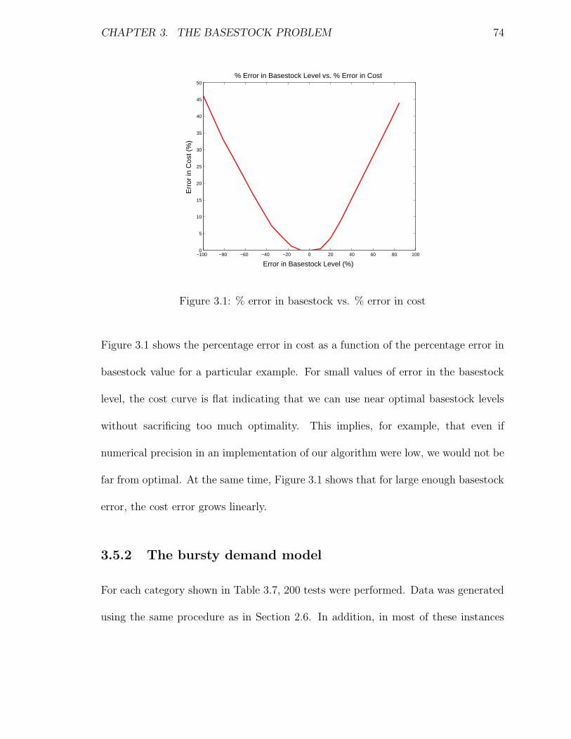
CHAPTER 3. THE BASESTOCK PROBLEM 74
−100 −80 −60 −40 −20 0 20 40 60 80 1000
5
10
15
20
25
30
35
40
45
50
Error in Basestock Level (%)
Err
or in
Cos
t (%
)
% Error in Basestock Level vs. % Error in Cost
Figure 3.1: % error in basestock vs. % error in cost
Figure 3.1 shows the percentage error in cost as a function of the percentage error in
basestock value for a particular example. For small values of error in the basestock
level, the cost curve is flat indicating that we can use near optimal basestock levels
without sacrificing too much optimality. This implies, for example, that even if
numerical precision in an implementation of our algorithm were low, we would not be
far from optimal. At the same time, Figure 3.1 shows that for large enough basestock
error, the cost error grows linearly.
3.5.2 The bursty demand model
For each category shown in Table 3.7, 200 tests were performed. Data was generated
using the same procedure as in Section 2.6. In addition, in most of these instances
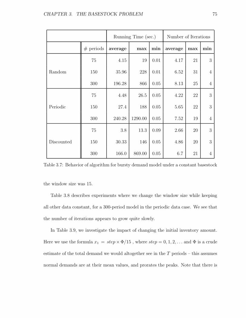
CHAPTER 3. THE BASESTOCK PROBLEM 75
Running Time (sec.) Number of Iterations
# periods average max min average max min
Random
75 4.15 19 0.01 4.17 21 3
150 35.96 228 0.01 6.52 31 4
300 196.28 866 0.05 8.13 25 4
Periodic
75 4.48 26.5 0.05 4.22 22 3
150 27.4 188 0.05 5.65 22 3
300 240.28 1290.00 0.05 7.52 19 4
Discounted
75 3.8 13.3 0.09 2.66 20 3
150 30.33 146 0.05 4.86 20 3
300 166.0 869.00 0.05 6.7 21 4
Table 3.7: Behavior of algorithm for bursty demand model under a constant basestock
the window size was 15.
Table 3.8 describes experiments where we change the window size while keeping
all other data constant, for a 300-period model in the periodic data case. We see that
the number of iterations appears to grow quite slowly.
In Table 3.9, we investigate the impact of changing the initial inventory amount.
Here we use the formula x1 = step×Φ/15 , where step = 0, 1, 2, . . . and Φ is a crude
estimate of the total demand we would altogether see in the T periods – this assumes
normal demands are at their mean values, and prorates the peaks. Note that there is
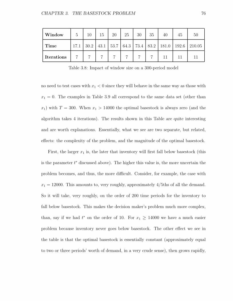
CHAPTER 3. THE BASESTOCK PROBLEM 76
Window 5 10 15 20 25 30 35 40 45 50
Time 17.1 30.2 43.1 53.7 64.3 73.4 83.2 181.0 192.6 210.05
Iterations 7 7 7 7 7 7 7 11 11 11
Table 3.8: Impact of window size on a 300-period model
no need to test cases with x1 < 0 since they will behave in the same way as those with
x1 = 0. The examples in Table 3.9 all correspond to the same data set (other than
x1) with T = 300. When x1 > 14000 the optimal basestock is always zero (and the
algorithm takes 4 iterations). The results shown in this Table are quite interesting
and are worth explanations. Essentially, what we see are two separate, but related,
effects: the complexity of the problem, and the magnitude of the optimal basestock.
First, the larger x1 is, the later that inventory will first fall below basestock (this
is the parameter t∗ discussed above). The higher this value is, the more uncertain the
problem becomes, and thus, the more difficult. Consider, for example, the case with
x1 = 12000. This amounts to, very roughly, approximately 4/5ths of all the demand.
So it will take, very roughly, on the order of 200 time periods for the inventory to
fall below basestock. This makes the decision maker’s problem much more complex,
than, say if we had t∗ on the order of 10. For x1 ≥ 14000 we have a much easier
problem because inventory never goes below basestock. The other effect we see in
the table is that the optimal basestock is essentially constant (approximately equal
to two or three periods’ worth of demand, in a very crude sense), then grows rapidly,
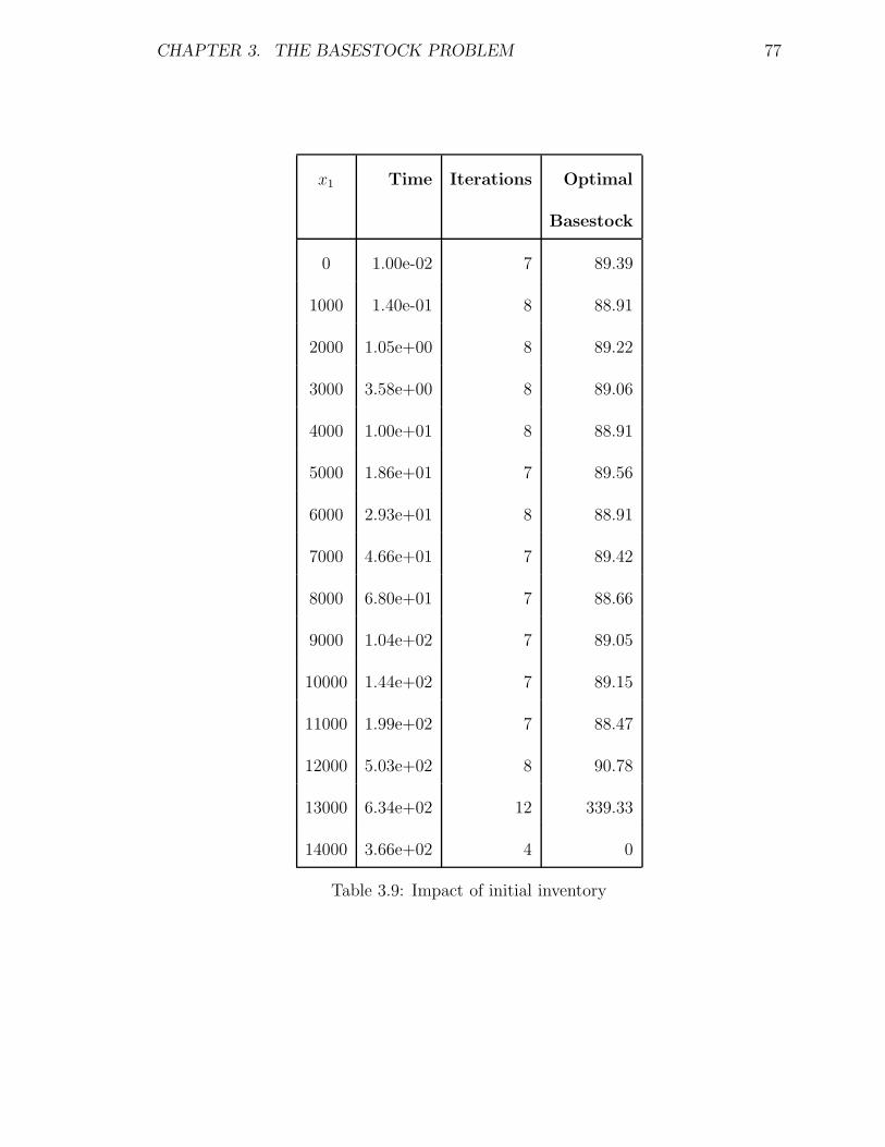
CHAPTER 3. THE BASESTOCK PROBLEM 77
x1 Time Iterations Optimal
Basestock
0 1.00e-02 7 89.39
1000 1.40e-01 8 88.91
2000 1.05e+00 8 89.22
3000 3.58e+00 8 89.06
4000 1.00e+01 8 88.91
5000 1.86e+01 7 89.56
6000 2.93e+01 8 88.91
7000 4.66e+01 7 89.42
8000 6.80e+01 7 88.66
9000 1.04e+02 7 89.05
10000 1.44e+02 7 89.15
11000 1.99e+02 7 88.47
12000 5.03e+02 8 90.78
13000 6.34e+02 12 339.33
14000 3.66e+02 4 0
Table 3.9: Impact of initial inventory
CHAPTER 3. THE BASESTOCK PROBLEM 78
and then drops to zero – when the initial inventory is large enough no “safety” is
needed. The sudden growth of the basestock at, or just before, the “critical” level
of x1 can be explained as follows: if x1 is large enough the risk that inventory will
go below basestock is low, until near the end of the planning horizon – so setting a
larger basestock value is unlikely to have a negative effect (i.e., ordering costs) until
near the end. However, for t near T the inventory could actually go negative, and a
larger basestock will protect against that.
Another important issue is how the optimal robust basestock behaves as a function
of the input data, and, in particular, as a function of how “large” the uncertainty
sets are. Table 3.10 demonstrates an interesting phenomenon that is also observed in
stochastic inventory theory (see [GKR05]). Here we have an example of the bursty
demand model. Our experiment consisted in scaling the window size parameter and
the magnitudes of the peaks by the same constant. Notice that by doing so we increase
the variability in the system. To understand the intuition behind this suppose that
Pt = P for all t. Then, on average, the peak demand at any period in window of size
w will be P/w, but the variance will be of the order of P 2/w. Hence, the “expected”
demand per period will not change if we scale the window and peak size by the same
constant, but demand variance will increase. Table 3.10 shows that as the variance
of the demand increases, the optimal basestock level initially increases, but then it
decreases and appears to converge to a constant.
We performed some additional tests to measure the sensitivity of the optimal
CHAPTER 3. THE BASESTOCK PROBLEM 79
Scale 0.4 0.6 0.8 1.0 1.2 1.4 1.6 1.8 2.6
Opt. Bs. 74.92 78.10 75.30 119.98 125.63 131.54 74.29 74.29 74.21
Table 3.10: Variance vs Optimal Basestock
0 0.2 0.4 0.6 0.8 1 1.2230
240
250
260
270
280
290
300
310Scale Factor vs Optimal Basestock Level
Scale
Bas
esto
ck L
evel
Figure 3.2: Effect of scaling peaks on optimum basestock
basestock to problem data, in particular to the magnitude of the peaks Pt. In these
tests we varied the problem data by scaling all peaks by the same scale constant, and
keeping all other data constant. Figure 3.2 displays the result of such a test on a
problem with T = 75, and window parameter W = 5.
Note that as the scale factor goes to zero the optimum basestock converges to a
constant. This is easy to understand, since when the peaks are small the adversary
does not gain much from using or not using the peaks. When the scale factor is
CHAPTER 3. THE BASESTOCK PROBLEM 80
large enough, the optimum basestock also converges to a constant. At first glance
this might appear incorrect: perhaps the optimum basestock should also increase, to
offset potential large backlogging costs? However, this view is incorrect, because if
we set the basestock large, then we have to carry large inventory in all periods.
3.6 Extensions
There are many possible extensions of the work described above which could prove
fruitful. We will describe some problem areas for which we have theoretical results.
3.6.1 Polyhedral uncertainty sets
In this paper we considered two models of demand uncertainty. Both models are
polyhedral (in the bursty demand case, we need additional variables). Certainly
one could consider generalizing our Benders’ decomposition approach to a general
polyhedral set D. In order to do so, we would need to develop a generic adversarial
problem solver.
From a practical standpoint, what seems to make most sense to us would be to
formulate the adversarial problem as a mixed-integer program, much like that in
Section 2.4.2 but adapted to the basestock or safety stock case. Of course, we would
also need to develop an algorithm (e.g. a branch-and-cut algorithm) for solving such
a problem – this will be an area for future work.
CHAPTER 3. THE BASESTOCK PROBLEM 81
From a purely theoretical standpoint, we can provide a negative result. We are
somewhat uncomfortable with this result, primarily because “in practice” the number
T would not be large. Nevertheless, the result is:
Theorem 3.6.1 Let G be a graph with n vertices and clique number κ(G). Then
there is a robust basestock problem with n + 1 periods and polyhedral uncertainty set
D, with value equal to κ(G).
Proof. See Section B.2.
There is a practical consequence to this theorem. Namely, it is known that unless
P = NP , there no polynomial-time algorithm that computes an approximation to
clique number guaranteed to have constant multiplicative error. Hence, unless P =
NP , there can not exist any polynomial-time algorithm that approximates the robust
basestock problem within any constant factor.
3.6.2 Robust safety stocks
In the standard probabilistic setting, if the demand at period t has mean µt and
standard deviation δt, a safety stock policy is a basestock policy with basestock σt =
µt + λ δt. We will refer to the quantity λ as the margin. In this section we consider
the problem of optimally choosing λ in a robust setting. In principle, the demand
uncertainty models we have considered allow us to compute adequate stand-ins for
µt and δ; however, for greater generality, we will assume that we are given quantities
CHAPTER 3. THE BASESTOCK PROBLEM 82
µt and δt for each t, and we want to optimally set a policy with basestock µt + λ δt.
Further, the problem could generalized by asking that λ = λt, but here we will restrict
ourselves to the constant case (though, of course, in practice we would consider the
rolling horizon implementation).
Formally, given parameters λl and λu, and an uncertainty set D, we want to solve the
problem:
minλl≤λ≤λu
F (λ) (3.33)
where, given λ,
F (λ) = maxd,x,u
T∑
t=1
( ctut + Wt(xt+1)) (3.34)
s.t.
ut = maxµt + λδt − xt , 0, 1 ≤ t ≤ T, (3.35)
xt+1 = xt + ut − dt, 1 ≤ t ≤ T, (3.36)
(d1, d2, . . . , dT ) ∈ D. (3.37)
To this end we propose the use of Algorithm 1.2.1. In this context, the decision
maker’s problem is that of choosing λ so as to minimize the maximum cost arising
from the use of margin λ when the demand vector is one of a finite set of possible
vectors. For a vector d of demands, let cost(λ, d) be the cost that ensues when we
use margin λ and the demands are d.
CHAPTER 3. THE BASESTOCK PROBLEM 83
Theorem 3.6.2 Let d be a fixed demand vector. Then cost(λ, d) is piecewise convex
with O(T 2) pieces, each of which is piecewise-linear.
Proof. First, let us add a “dummy” period, T +1, with hT+1 = bT+1 = cT+1 = 0, and
with µT+1 and δT+1 chosen so that µT+1 + λδT+1 ≥ x1 and µT+1 + λδT+1 ≥ µt + λδt
for every t ≤ T and every λ ∈ [λl, λu]. [remark: it is clear that it is always possible
to find such parameters µT+1, δT+1; the choice guarantees guarantees that xT+1 ≤
µt+1 + λδT+1].
Let 1 ≤ t1 < t2 ≤ T + 1 be given. Consider the following system of equations:
µt1 + λδt1 −i∑
j = t1
dj ≥ µi+1 + λδi+1, t1 ≤ i ≤ t2 − 2, (3.38)
µt1 + λδt1 −t2−1∑
j = t1
dj ≤ µt2 + λδt2 . (3.39)
The interpretation of this system is as follows. Suppose that at time t1 the starting
inventory is at or below basestock. Then if λ satisfies (3.38) and (3.39), in periods
t1 +1, t1 +2, . . . , t2− 1 inventory will be above or equal basestock, but in period t2 it
will once again below or equal basestock. Note that there are constants α1L(t1, t2) and
α1U(t1, t2) such that λ satisfies (3.38) and (3.39) if and only if λ ∈ [α1
L(t1, t2), α1U(t1, t2)]
(possibly, the α are infinite).
Similarly, for 1 ≤ t < T + 1, consider the system:
µt + λδt − dt ≤ µt+1 + λδt+1, (3.40)
with a similar interpretation, and defining an interval [α2L(t), α2
U(t)]. Finally, for each
CHAPTER 3. THE BASESTOCK PROBLEM 84
2 ≤ t ≤ T + 1, consider the system
x1 ≥ µ1 + λδ1 (3.41)
x1 −i∑
j =1
dj ≥ µi + λδi 1 ≤ i ≤ t− 2, (3.42)
x1 −t−1∑
j =1
dj ≤ µt + λδt, (3.43)
again with a similar interpretation, and corresponding to some interval [α3L(t), α3
U(t)].
Let N be the total number of (finite) distinct values α, and let β1 < β2 < . . . < βN
denote the sorted list of such values. Write β0 = −∞, βN+1 = +∞. Then, it is clear
that in each open interval (βj, βj+1) the behavior of the system is fixed. More precisely,
if we take two distinct margin values λ1, λ2, both in (βj, βj+1), then inventory will be
over (resp., under) basestock in exactly the same periods under policy λ1 as under
policy λ2.
It follows that total cost (including ordering cost), as a function of λ, is convex
piecewise-linear for λ ∈ (βj, βj+1). Since N = O(T 2) the result is proved.
Corollary 3.6.3 Given a finite set of demand patterns D, the decision maker’s prob-
lem can be solved in polynomial time, by minimizing a piecewise convex function with
O(T 2D) pieces.
Now we turn to the adversarial problem, which we cast in the following context:
we are given basestock levels σ1, σ2, . . . , σT . We want to find a demand vector d ∈ D
that maximizes the cost that would ensue from using the basestock policy σtt. We
CHAPTER 3. THE BASESTOCK PROBLEM 85
expect that both the risk budgets model and the bursty demands model will prove
computationally tractable in this general setting, even though they are likely NP-
hard (we already know this for the bursty demands model). We will return to this
point below. We do have a positive theoretical result for an uncertainty model that
amounts to a discrete version of the risk budgets model.
The model is described as follows:
(a) We are given a quantity 0 ≤ µt for 1 ≤ t ≤ T . This is the nominal demand at
time t.
(b) We are given quantities αi ≥ 0, for 1 ≤ i ≤ C (some C).
(c) Each time period t belongs to a category i, 1 ≤ i ≤ C. If period t is in category
i, then the demand at t will be of the form
dt = µt + kt αi, (3.44)
where kt is an integer, possibly negative. We have bounds lt ≤ kt ≤ ut for given
lt, ut.
(d) For each t we have a constraint of the form∑t
j=1 |kj| ≤ Γt, where 0 ≤ Γt is a
given integer. (We assume that ΓT is polynomial in T ).
Comments. We may view each category as describing a variance “class” or “type”.
The weakness of (3.44) is, of course, that ideally we would have instead a mechanism
CHAPTER 3. THE BASESTOCK PROBLEM 86
of the form dt = µt + kt αi,t. But, for example, in a setting with seasonal demands,
the above model should prove functional. We will refer to the model as the discrete
budgets model. One can prove the following result, which is primarily of theoretical
relevance.
Theorem 3.6.4 Given a basestock policy with levels σtt, the adversarial problem
under a discrete budgets model can be solved in polynomial time, for each fixed C.
Proof. See Section C.1.
We say that this result is only of theoretical importance, because the adversarial
problem appears to be “knapsack-like”, and hence an algorithm such as the one we
described for the bursty demands model in Section 3.4 would prove far more practical
(though nominally of exponential complexity since it solves mixed-integer programs).
If anything, the fact that Theorem 3.6.4 can be proved would justify such an approach.
Next we list generalizations of the discrete budgets model that are also likely to be
numerically tractable:
• A discrete model with demands of the form dt = µt + kt αi,t, where kt is
integral, and we have budgets of the form∑t
j=1 |kj| ≤ Γt (as discussed above).
• A model where, for every t, we are given µt, and quantities 0 < α0t < α1
t <
. . . < αU(t)t , and quantities 0 < β0
t < β1t < . . . < β
L(t)t , for some U(t) and
L(t). At time t, the adversary chooses an integer kt, with either 0 < kt ≤
CHAPTER 3. THE BASESTOCK PROBLEM 87
U(t), or 0 < −kt ≤ L(t), or kt = 0. If kt > 0, then demand will be in
the interval (µt + αkt−1t , µt + αkt
t ]. If kt < 0, then demand will be in the
interval [µt − β−ktt , µt − β−kt−1
t ). If the adversary chooses 0, then demand lies
in [µt − β0t , µt + α0
t ]. Once more we have budgets∑t
j=1 kj ≤ Γt.
In all the above models we were using budget constraints motivated by the original
risk budgets model in [BT04]. But there is a generalization, which we call the intervals
model, which still proves tractable. We explain this generalization in the context of
the discrete budgets model, but it is easily extended to the original (continuous) risk
budgets setting. First, we are given quantities αi ≥ 0, for 1 ≤ i ≤ C (some C), and
demand at time t is of the form dt = µt + kt αi as for the discrete budgets model. In
addition, we are given
• A family I of closed intervals of 1, 2, . . . , T, and a nonnegative integer ΓI for
each I ∈ I.
• We must satisfy∑
t∈I |kt| ≤ ΓI , for each I ∈ I.
We will say that an interval model with family I is of width≤ ω, if there exist intervals
[i1, j1], . . . , [im, jm], of 1, 2, . . . , T such that:
(i) I is the set of all intervals of the form [ik, h] for some 1 ≤ k ≤ m and ik ≤ h ≤ jk,
and
(ii) For every 1 ≤ t ≤ T there are at most ω intervals [ik, jk] with ik ≤ t ≤ jk.
CHAPTER 3. THE BASESTOCK PROBLEM 88
We call the intervals [i1, j1], . . . , [im, jm] basis for set I. We say that the model has
width ω if the condition in (ii) holds with equality for some t. Note that a model
of width ω = 2 can be made substantially more restrictive on the adversary than
one with ω = 1. The following result can be proved, again primarily of theoretical
relevance:
Theorem 3.6.5 Suppose we have a basestock policy with levels σtt. Suppose we
have an interval model of width ≤ ω, and with C variance types. Then, for each fixed
ω and C, the adversarial problem can be solved in polynomial time
Proof. See Section C.2 .
3.6.3 Ambiguous uncertainty sets
In the ambiguous setting demands are known to follow some probabilistic distribution,
but the decision maker only has limited information regarding the distribution. For
example, we might know that the distribution (at any time t) is log-normal, and we
might know its mean value, but might only know an upper bound on the variance.
Conceptually, we may think of the adversary as choosing a probability distribution on
the demands that is consistent with the available information. This yields a problem
of the form:
minπ∈Π
maxP∈P
E cost(π|P ).
CHAPTER 3. THE BASESTOCK PROBLEM 89
Here, Π is the set of available policies, P is the set of possible probability distribu-
tions, and E cost(π|P ) is the expected cost, under policy π when the demands follow
distribution P . To solve this problem, we can again resort to a generic Benders’
decomposition method obtained by suitably modifying Algorithm 1.2.1.
Here we focus on basestock policies.
Lemma 3.6.6 Let σ be a given basestock and let P be a probability distribution. (a) If
x1 ≤ 0, then E cost(σ|P ) is a convex function of σ. (b) If P is a discrete distribution,
then E cost(σ|P ) is piecewise convex.
Proof. To prove part (a) notice that for a fixed demand pattern d, cost of using
basestock level σ is equal to
c1(σ − x1) +T∑
i=1
(ci+1di + maxhi(σ − di), bi(di − σ))
which is a convex function of σ. Therefore, E cost(σ|P ) will be a convex function of
σ.
For part (b), consider Lemma 3.2.3. This Lemma states that for a fixed demand
pattern d, cost is a piecewise convex function of σ with two pieces. Therefore if P
has a discrete distribution, E cost(σ|P ) is a piecewise convex function of σ. (If the
distribution has a finite support, then the number of convex pieces will also be finite.)
In part (b) of the above Lemma, and in the results we describe next, we focus on
CHAPTER 3. THE BASESTOCK PROBLEM 90
a particular model of ambiguous uncertainty, namely the discrete distribution model.
Here
• we are given fixed values v1, v2, . . . , vK,
• The adversary will choose probabilities pk, 1 ≤ k ≤ K, such that in any time
period demand equals vk with probability pk.
• It is assumed that the adversary is constrained in that the vector (p1, . . . , pk)
must belong to some set P (for example, polyhedral).
Lemma 3.6.7 Let P 1, P 2, . . . , P J be given discrete probability distributions. Suppose
that x1 ≤ 0. Then we can compute, in polynomial time, a basestock σ that minimizes
max1≤j≤J E cost(σ|P j).
Proof. Consider a fixed distribution P j. Note that since x1 ≤ 0, the expected
inventory cost paid in every period is the same. Also, the expected ordering cost paid
in any period, other than period 1, is the same (and in period 1 it equals σ − x1).
Further, if demand equals vk ≥ σ then we incur a backlogging cost, otherwise we
incur an inventory holding cost. Hence, we can write a closed form expression on
E cost(σ|P j), which will be piecewise linear in σ (and is convex because of Lemma
3.6.6). The result follows.
Comment. The assumption x1 ≤ 0 is significant. Without the assumption we can
prove a result similar to Lemma 3.6.7, except that the resulting algorithm will be
exponential in K.
CHAPTER 3. THE BASESTOCK PROBLEM 91
Lemma 3.6.8 Let σ be given, and assume x1 ≤ 0. Then the adversarial problem
reduces to maximizing a linear function of (p1, . . . , pk) over (p1, . . . , pk) ∈ P.
Proof. Notice that the adversarial problem reduces to maximizing the following func-
tion.
E
[
T∑
i=1
(ci+1di + maxhi(σ − di), bi(di − σ))
]
=T∑
i=1
E [ ci+1di + maxhi(σ − di), bi(di − σ) ]
Since each of the terms inside the second sum is a linear function of (p1, . . . , pk), the
result follows.
A variation worth noting is the rolling horizon model. But here we can expect that
the decision maker learns from the past behavior of the adversary; i.e. the knowledge
of the set P is sharpened. To be fair, one should then consider a gaming setting where
the adversary can respond in kind.
3.6.4 Model superposition
Suppose we have a number of demand uncertainty sets D1, D2, . . . ,DK, and for each
k = 1, . . . , K, cost vectors hk, bk, ck (e.g. hk = (hk1, h
k2, . . . , h
kT and similarly with bk
and ck). Let Π be a set of available policies. We are interested in a problem of the
form:
minπ∈Π
maxk
maxd∈Dk
costk(π, d), (3.45)
CHAPTER 3. THE BASESTOCK PROBLEM 92
(where costk is the cost under the kth cost function), or
minπ∈Π
∑
k
maxd∈Dk
costk(π, d). (3.46)
As a generalization, we could have that some of the Dk are ambiguous problems, or
even stochastic programs. In all these cases our generalized Benders’ methodology
applies. We are motivated to study these problems for a number of reasons:
• Consider a case where D1 ⊆ D2 ⊆ . . . ⊆ DK and there are vectors h, b, c and
nonnegative constants α1 ≥ α2 ≥ . . . ≥ αK , such that (hk, bk, ck) = αk (h, b, c).
In other words, each uncertainty set Dk is more conservative than Dk−1, but its
cost “counts less”. Problems (3.45) and (3.46) are an attempt to protect against
potentially very poorly behaved data (demands) without becoming excessively
conservative. A special example of this case is that where the Dk all have the
same structural properties (for example, they are all box-constrained in each
time period).
• On the other hand, if the sets Dk are extremely different and/or so are the cost
functions, then we are simply trying to protect against multiple forms of data
uncertainty, again while trying to avoid becoming too conservative.
• Finally, we conjecture that using relatively simple sets Dk, and not very large
K, one should be able to approximate arbitrarily complex uncertainty sets D,
so that e.g. solving (3.45) becomes more tractable than solving (1.1).
CHAPTER 3. THE BASESTOCK PROBLEM 93
3.6.5 More comprehensive supply-chain models
The algorithms described in this paper addressed single-buffer, zero-leadtime prob-
lems. In a more realistic setting we should consider positive leadtime systems (e.g.
an order placed at time t does not arrive until time t + k). Multiple buffers arise,
for example, in assembly systems, where a product is obtained by assembling several
components, each of which is itself made of (sub)components, and so on. Here each
component has its own buffer and material flows from buffer to buffer on a network in
a prescribed sequence. Problems of this type with certain data can be solved under
appropriate assumptions (for example, involving coordination); in a robust setting
the problem is bound to be more complex, but it should be possible to adapt our
techniques so as to (at least) efficiently compute local optima.
3.7 Summary of the results
In this chapter we presented algorithms for solving the optimal robust basestock
problem (3.1) using two different models for the demand uncertainty set D. The
algorithms are based on our generic Bender’s decomposition procedure in Chapter 1.
Our results can be summarized as follows:
(i) Our algorithms compute optimal basestock levels, a problem of concrete prac-
tical importance due to widespread use. We solve the problems to proved opti-
mality, up to roundoff error. Further, we demonstrate, empirically, that using
CHAPTER 3. THE BASESTOCK PROBLEM 94
incorrect basestock settings can lead to a substantial cost increase.
(ii) In our numerical experiments we consider two models of demand uncertainty,
and in each case we solve the actual min-max optimization problem, and not
a conservative approximation. Despite the fact that we solve non-convex opti-
mization problems, extensive experimentation shows that our algorithms scale
well with problem size, typically solving problems with several hundred periods
in a few minutes of CPU time, in the worst case, and significantly faster in
many cases. Further, in the case of the hardest problems we consider, we also
describe an approximation scheme that produces solutions which are proved
near-optimal significantly faster.
(iii) All of our algorithms can be viewed as variations on Benders’ decomposition –
this approach should extend well to many demand uncertainty models.
(iv) We present theoretical results concerning robust safety-stock selection, and ex-
tensions to other models, such as ambigious uncertainty models (models where
the demand distribution is stochastic but only partially known to the decision
maker).
CHAPTER 4. THE DYNAMIC PROBLEM 95
Chapter 4
The Dynamic Problem
In this chapter we will consider the robust inventory management problem in the
dynamic setting. We allow our policy space to contain all policies, and thus in each
period the inventory controller will have the freedom to determine the orders as an
arbitrary function of the information that he has at that period. In other words,
for each period, a policy amounts to a function that gives the order amount for
any possible realization of the demands from previous periods. We assume that
the inventory controller wants to minimize the cost over all such ordering functions.
Instead of the generic algorithm that we introduced in Chapter 1, we use dynamic
programming to solve this problem.
Let (d1, d2, . . . , dt−1) be the vector of demands up to period t. We denote the
vector that contains information that one has at the beginning of period t prior to
placing the order by It = (xt, d1, d2, . . . , dt−1) and the set of all possible information
CHAPTER 4. THE DYNAMIC PROBLEM 96
vectors in period t is denoted by It. Further, we denote our decision rule in period t
for determining order quantities with πt(xt, d1, d2, . . . , dt−1). πt(xt, d1, d2, . . . , dt−1) is
a function from It to real numbers and in every period t, it specifies the amount of the
stock to be ordered in that period. We define the stock ordering policy, π to be the
sequence of decision rules, i.e. π = (πt(.) : t = 1, . . . , T ). Moreover, we denote the set
of all possible policies by Π. Notice that we can also think of the static policies and
dynamic problems in this context. The Static policies in Chapter 2 correspond to the
case in which the decision rule in each period t is defined by a constant function that is
πt(xt, d1, d2, . . . , dt−1) = ut for a real number ut ≥ 0 for every (xt, d1, d2, . . . , dt−1) ∈ It
whereas constant basestock policies in Chapter 3 correspond to the case where the
decision rule in each period t is of the form πt(xt, d1, d2, . . . , dt−1) = σ − xt.
The robust inventory problem in the dynamic setting can be described as follows:
minπ∈Π
V (π) (4.1)
where for π ∈ Π,
V (π) = maxd,x,u
T∑
t=1
( ctut + max htxt+1 , −btxt+1 ) (4.2)
s.t.
u1 ≥ 0
ut = πt(d1, d2, ..., dt−1), 2 ≤ t ≤ T, (4.3)
xt+1 = xt + ut − dt, 1 ≤ t ≤ T, (4.4)
(d1, d2, . . . , dT ) ∈ D. (4.5)
CHAPTER 4. THE DYNAMIC PROBLEM 97
Here, x1 is given and πt(.) is the ordering function specified by the policy π. We
dropped xt from the arguments of πt(.) since it is also a function of (d1, d2, . . . , dt−1)
and the given x1. Notice that (4.1) is of the same form as (3.1). The only difference
lies in the policy space: instead of time-independent basestock policies, we minimize
the cost over all policies.
In Section 4.2 we will give a characterization of the optimal policy. The optimal
policy turns out to be a state dependent basestock policy where the state space in
each period t is defined by It. (In each period t, the optimal policy will be a basestock
policy and the optimal basestock level will depend on the demand in prior periods).
From a practical standpoint, such policies are very hard to compute and implement
since the number of possible realizations of demand can be extremely large. However,
this problem is of interest, because it provides a justification for the use of time and
state independent basestock policy either by itself or in a rolling horizon fashion as
an approximation for the pure dynamic policies which is the ideal thing to do.
This chapter is organized as follows: We first prove that problem 4.1 can be solved
by dynamic programming in Section 4.1. In Section 4.2 we characterize the optimal
policies. We show how to compute optimal policies for the two demand uncertainty
sets in Sections 4.3 and 4.4.
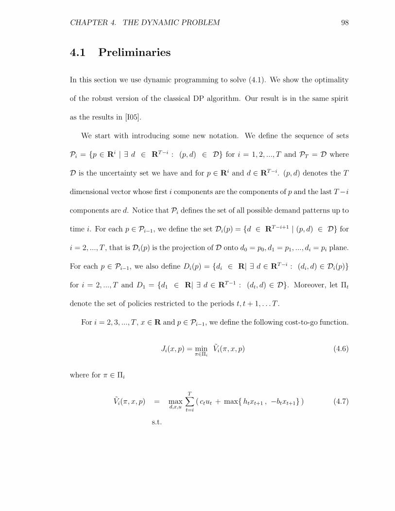
CHAPTER 4. THE DYNAMIC PROBLEM 98
4.1 Preliminaries
In this section we use dynamic programming to solve (4.1). We show the optimality
of the robust version of the classical DP algorithm. Our result is in the same spirit
as the results in [I05].
We start with introducing some new notation. We define the sequence of sets
Pi = p ∈ Ri | ∃ d ∈ RT−i : (p, d) ∈ D for i = 1, 2, ..., T and PT = D where
D is the uncertainty set we have and for p ∈ Ri and d ∈ RT−i. (p, d) denotes the T
dimensional vector whose first i components are the components of p and the last T−i
components are d. Notice that Pi defines the set of all possible demand patterns up to
time i. For each p ∈ Pi−1, we define the set Di(p) = d ∈ RT−i+1 | (p, d) ∈ D for
i = 2, ..., T , that is Di(p) is the projection of D onto d0 = p0, d1 = p1, ..., di = pi plane.
For each p ∈ Pi−1, we also define Di(p) = di ∈ R| ∃ d ∈ RT−i : (di, d) ∈ Di(p)
for i = 2, ..., T and D1 = d1 ∈ R| ∃ d ∈ RT−1 : (dt, d) ∈ D. Moreover, let Πt
denote the set of policies restricted to the periods t, t + 1, . . . T .
For i = 2, 3, ..., T , x ∈ R and p ∈ Pi−1, we define the following cost-to-go function.
Ji(x, p) = minπ∈Πi
Vi(π, x, p) (4.6)
where for π ∈ Πi
Vi(π, x, p) = maxd,x,u
T∑
t=i
( ctut + max htxt+1 , −btxt+1 ) (4.7)
s.t.
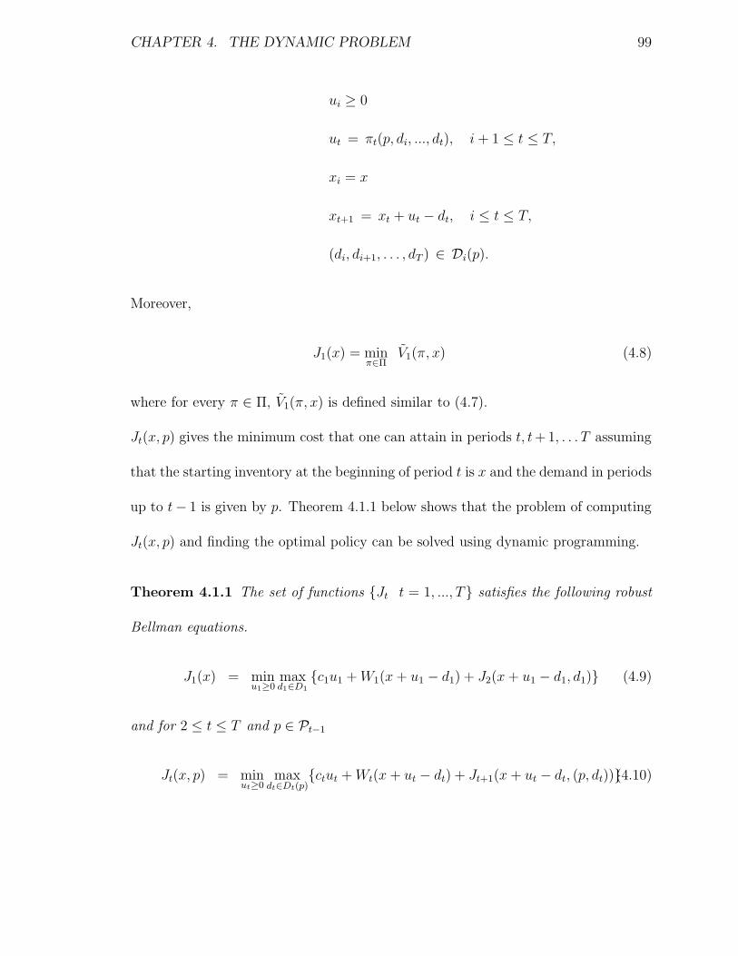
CHAPTER 4. THE DYNAMIC PROBLEM 99
ui ≥ 0
ut = πt(p, di, ..., dt), i + 1 ≤ t ≤ T,
xi = x
xt+1 = xt + ut − dt, i ≤ t ≤ T,
(di, di+1, . . . , dT ) ∈ Di(p).
Moreover,
J1(x) = minπ∈Π
V1(π, x) (4.8)
where for every π ∈ Π, V1(π, x) is defined similar to (4.7).
Jt(x, p) gives the minimum cost that one can attain in periods t, t+1, . . . T assuming
that the starting inventory at the beginning of period t is x and the demand in periods
up to t− 1 is given by p. Theorem 4.1.1 below shows that the problem of computing
Jt(x, p) and finding the optimal policy can be solved using dynamic programming.
Theorem 4.1.1 The set of functions Jt t = 1, ..., T satisfies the following robust
Bellman equations.
J1(x) = minu1≥0
maxd1∈D1
c1u1 + W1(x + u1 − d1) + J2(x + u1 − d1, d1) (4.9)
and for 2 ≤ t ≤ T and p ∈ Pt−1
Jt(x, p) = minut≥0
maxdt∈Dt(p)
ctut + Wt(x + ut − dt) + Jt+1(x + ut − dt, (p, dt))(4.10)
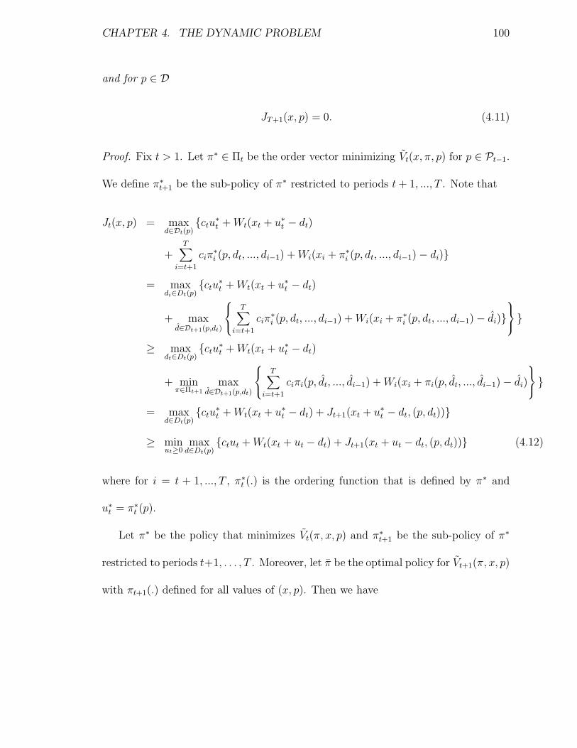
CHAPTER 4. THE DYNAMIC PROBLEM 100
and for p ∈ D
JT+1(x, p) = 0. (4.11)
Proof. Fix t > 1. Let π∗ ∈ Πt be the order vector minimizing Vt(x, π, p) for p ∈ Pt−1.
We define π∗t+1 be the sub-policy of π∗ restricted to periods t + 1, ..., T . Note that
Jt(x, p) = maxd∈Dt(p)
ctu∗t + Wt(xt + u∗
t − dt)
+T∑
i=t+1
ciπ∗i (p, dt, ..., di−1) + Wi(xi + π∗
i (p, dt, ..., di−1)− di)
= maxdi∈Dt(p)
ctu∗t + Wt(xt + u∗
t − dt)
+ maxd∈Dt+1(p,dt)
T∑
i=t+1
ciπ∗i (p, dt, ..., di−1) + Wi(xi + π∗
i (p, dt, ..., di−1)− di)
≥ maxdt∈Dt(p)
ctu∗t + Wt(xt + u∗
t − dt)
+ minπ∈Πt+1
maxd∈Dt+1(p,dt)
T∑
i=t+1
ciπi(p, dt, ..., di−1) + Wi(xi + πi(p, dt, ..., di−1)− di)
= maxd∈Dt(p)
ctu∗t + Wt(xt + u∗
t − dt) + Jt+1(xt + u∗t − dt, (p, dt))
≥ minut≥0
maxd∈Dt(p)
ctut + Wt(xt + ut − dt) + Jt+1(xt + ut − dt, (p, dt)) (4.12)
where for i = t + 1, ..., T , π∗t (.) is the ordering function that is defined by π∗ and
u∗t = π∗
t (p).
Let π∗ be the policy that minimizes Vt(π, x, p) and π∗t+1 be the sub-policy of π∗
restricted to periods t+1, . . . , T . Moreover, let π be the optimal policy for Vt+1(π, x, p)
with πt+1(.) defined for all values of (x, p). Then we have
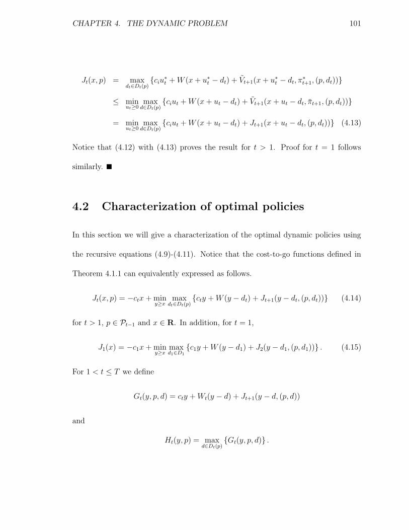
CHAPTER 4. THE DYNAMIC PROBLEM 101
Jt(x, p) = maxdt∈Dt(p)
ciu∗t + W (x + u∗
t − dt) + Vt+1(x + u∗t − dt, π
∗t+1, (p, dt))
≤ minut≥0
maxd∈Dt(p)
ciut + W (x + ut − dt) + Vt+1(x + ut − dt, πt+1, (p, dt))
= minut≥0
maxd∈Dt(p)
ciut + W (x + ut − dt) + Jt+1(x + ut − dt, (p, dt)) (4.13)
Notice that (4.12) with (4.13) proves the result for t > 1. Proof for t = 1 follows
similarly.
4.2 Characterization of optimal policies
In this section we will give a characterization of the optimal dynamic policies using
the recursive equations (4.9)-(4.11). Notice that the cost-to-go functions defined in
Theorem 4.1.1 can equivalently expressed as follows.
Jt(x, p) = −ctx + miny≥x
maxdt∈Dt(p)
cty + W (y − dt) + Jt+1(y − dt, (p, dt)) (4.14)
for t > 1, p ∈ Pt−1 and x ∈ R. In addition, for t = 1,
J1(x) = −c1x + miny≥x
maxd1∈D1
c1y + W (y − d1) + J2(y − d1, (p, d1)) . (4.15)
For 1 < t ≤ T we define
Gt(y, p, d) = cty + Wt(y − d) + Jt+1(y − d, (p, d))
and
Ht(y, p) = maxd∈Dt(p)
Gt(y, p, d) .
CHAPTER 4. THE DYNAMIC PROBLEM 102
For t = 1 we define G1(y, d) and Ht(y) in a similar way. We have the following
theorem.
Theorem 4.2.1
(a) For fixed t and p ∈ Pt−1, Ht(y, p) is a convex function of y.
(b) For the first period the optimal policy is a basestock policy. For each period t > 1
and each p ∈ Pt−1 there exists a basestock level, St,p such that it is optimal to order
St − xt if St > xt and it optimal not to order when St ≤ xt where xt is the inventory
at the beginning of period t.
(c) For t > 1 Jt(x, p) is a convex function of x for fixed p and J1(x) is a convex
function of x.
Proof. We prove the theorem by induction. For t = T and fixed p ∈ PT−1,
GT (y, p, d) = cT y + W (y − d)
is a convex function of y. Since HT (y, p) is the maximum of a set of convex functions
it is also convex. Let ST (p) be the smaller minimizer of HT (y, p) for fixed p. Note
that y = x, and y = ST (p), minimize Ht(y, p) over the set y : y ≥ x when x > ST
and x ≤ ST (p), respectively, and this proves part (b). Convexity of JT (x, p) with
respect to x follows from the fact that JT (x) = −cx + HT (max(ST , x), p), which is
the sum of a linear function and the composition of a convex function with another
convex function.
CHAPTER 4. THE DYNAMIC PROBLEM 103
Now assume that theorem is true for t + 1. Consider Gt(y, p, d) for fixed p and
d. Note that first two terms are a constant and a piecewise linear, convex function.
Moreover, from the induction hypothesis Jt+1(x, (p, dt)) is a convex function of x, so
it is also a convex function of y. Consequently, Ht(y, p) is a convex function of y for
fixed p.
Part (b) and (c) follows from part (a) and as in the base case. Proof for t = 1 also
follows similarly.
Theorem 4.2.1 states that in each period t, for every realization of the past de-
mands we have a different basestock level. The reason for this is that our uncertainty
set in each period t, Dt(p) depends on the vector of past demands, p. For different
p ∈ Pt−1, the available demand patterns for the adversary may be different. There-
fore, for each policy, the future demand that maximizes cost may be different for
different realizations of the past demand which clearly means that optimal policy will
be dependent on past demand.
For each period t the demand vector p takes values from Pt−1 which may have
infinitely many elements. In order to solve the problem, we may have to compute
an infinite number of basestock levels for every possible value of p. However, notice
that the optimal policy depends on p only through Dt(p) in each period t. Therefore
for any vectors p1 6= p2, the optimal policies for these two vectors are the same if
Dt(p1) = Dt(p2). We will use this fact in order to decrease the number of optimal
basestocks we have to compute.
CHAPTER 4. THE DYNAMIC PROBLEM 104
To solve the dynamic program in Theorem 4.1.1, we have compute the cost-to-go
function in for all values of the state variable which, for each period t, consists of
(x,p) such that x ∈ R and p ∈ Pt−1. Although we may be able to diminish the size
of our state space by using some properties of our uncertainty set, it may still be
very large in most cases and directly applying the dynamic programming algorithm
will be impractical due to its computational burden. However, the optimality of
state dependent basestock policies gives a justification for the use of time and state
independent basestock policies as an approximation.
One advantage of using the dynamic approach is that we can incorporate a fixed
ordering cost into our model without too much a large increase the computational
complexity. In fact, using the dynamic programming approach one can prove that in
the fixed cost case, the optimal policy is a two parameter basestock policy (an (S,s)
policy) where the basestock parameters again depend on the state variables.
4.3 Risk budgets model
In this section we will show how to solve the dynamic problem for the demand model
(2.3)-(2.5).
Let d and d two demand patterns in our demand uncertainty sets, and z and z
the corresponding vectors defined according to the equation (2.3). Let dt, dt, zt and
CHAPTER 4. THE DYNAMIC PROBLEM 105
zt be the subvectors restricted to periods 1, . . . , t for some t < T . If
t∑
i=1
zti =
t∑
i=1
zti
we have Dt+1(dt) = Dt+1(d
t), so Jt+1(x, dt) = Jt+1(x, dt) for any x. Therefore we can
replace the second argument which is the past demand in the cost-to-go function with
the total risk consumed up to that period (which is equal to the sum of z’s). As a
result the dynamic programming recursion turns into the following form.
J1(x) = minu1≥0
maxd1∈D1
c1u1 + W (x + u1 − d1) + J1(x + u1 − d1,
∣
∣
∣
∣
∣
d1 − µ1
δ1
∣
∣
∣
∣
∣
)
and for 2 ≤ t ≤ T and 0 ≤ k ≤ Γt−1
Jt(x, k) = minut≥0
maxdt∈Dt(k)
ctut + W (x + ut − dt) + Jt+1(x + ut − dt, k +
∣
∣
∣
∣
∣
dt − µt
δt
∣
∣
∣
∣
∣
)
and for 0 ≤ k ≤ ΓT
JT+1(x, k) = 0.
where Dt(k) is defined similarly to Dt(p) which is defined in Section 4.1. Here Jt(x, k)
for t > 1 gives the optimal total cost for periods t, . . . , T assuming that the risk used
up until period t− 1 is k and the starting inventory in period t is x.
Although our state space has two dimensions now, we still have to compute com-
pute the cost-to-go function for any value of risk usage which is in [0, Γt] which means
that we can only approximate the true cost-to-go by discretization. But once we
discretize k, it is possible to show that for a fixed risk consumption the cost-to-go
CHAPTER 4. THE DYNAMIC PROBLEM 106
function is piecewise linear in x, and therefore as in the algorithm for the adversarial
problem in Chapter 2, we can compute the function by evaluating each of its pieces.
4.3.1 A special case
The dynamic programming algorithm proves to be efficient when uncertainty set is
described by the condition dt ∈ [µt − δt, µt + δt] (which means Γt = t in our risk
budgets context). This model is the box model that we considered in Section 2.4.1.
Notice that we can get rid of the second argument in the cost-to-go function, since
no matter what the past demand is, we always have the same uncertainty set for the
future periods and Dt(p) = [µt−δt, µt +δt] for every p and t. In fact, due to convexity
of the cost function, it is easy to see that in the optimal solution, the adversary sets
either dt = µt− δt or dt = µt + δt for each t. Therefore, the cost-to-go functions turns
out to be as follows. For 1 ≤ t ≤ T
Jt(x) = minut≥0
maxdt∈µt−δt,µt+δt
ctut + W (x + ut − dt) + Jt+1(x + ut − dt)
and JT+1(x) = 0.
Using Lemma 2.4.4, we have the following result:
Lemma 4.3.1
(a) For every t, Jt(x) is a piecewise linear convex function with T − t + 2 pieces.
(b) The dynamic program for the box model can solved in O(T 2) time.
CHAPTER 4. THE DYNAMIC PROBLEM 107
We want to emphasize the fact that the optimal policy in the dynamic setting is
a state dependent basestock policy. The reason for the dependence on state space is
due to the dependence of future demands that is picked by the adversary on the past
demands. In the box uncertainty case, however, the adversary’s behavior behavior
is independent from the demand history. Thus, basestock levels will only depend on
time, not the state of the system.
4.4 Bursty demand model
In this section we consider the adversarial problem for the bursty demand model given
in Section 2.2. We can adapt the dynamic programming recursion used for the risk
budgets model as follows.
For each period t, and each integer 1 ≤ k < minW, t, let Πt(x, k), denote the
minimum cost attainable in periods t, . . . , T assuming that the initial inventory at
the start of period t is x, and that the last peak occurred in period t− k. Similarly,
denote by Πt(x, 0) the minimum cost attainable in periods t, . . . , T assuming that the
initial inventory at the start of period t is x, and that no peak occurred in periods
t− 1, t− 2, . . . , max1, t−W + 1. Writing ΠT+1(x, k) = 0, we have, for 1 ≤ t ≤ T :
Πt(x, k) = minut≥0
maxd∈µt−δt,µt+δt
ctut +Wt(x + ut − d) + Πt+1(x + ut − d, k + 1) ,
CHAPTER 4. THE DYNAMIC PROBLEM 108
for 1 ≤ k < minW − 1, t
Πt(x, W − 1) = minut≥0
maxd∈µt−δt,µt+δt
ctut +Wt(x + ut − d) + Πt+1(x + ut − d, 0) ,
for W − 1 < t,
Πt(x, 0) = minut≥0
max
Π1t (x), Π0
t (x)
, where
Π1t (x) = min
ut≥0max
d∈µt−δt,µt+δtctut +Wt(x + ut − d) + Πt+1(x + ut − d, 0) ,
Π0t (x) = ctut +Wt(x + ut − Pt) + Πt+1(x + ut − Pt, 1).
To solve the recursions above one can use the same approach with the budgets model.
For each k we compute and store the piecewise linear representation of Πt(x, k).
Moreover, from Theorem 4.2.1, the optimal policy is a basestock policy that in each
period t, depends on the last peak that occurred before t.
Appendix A
An alternative approach for solving
PM
In this section we present an alternative method to solve problem PM(γ, t∗, tf , te),
iteratively for different values of γ and te. Originally, in Section 3.3.4 we described a
dynamic programming method to solve the problem. Note that in the formulation in
section 3.3.1 the right hand side values of (3.14)-(3.16) are integral. For simplicity, we
re-index the problem and set Γi−t∗+1(γ) = bΓi−γc for i ∈ t∗, ..., tf − 2, Γtf−t∗(γ) =
minbΓtf − (γ + l(γ, te))c, bΓtf−1 − γc), and Γi−t∗(γ) = bΓi − (γ + l(γ, te))c for
i ∈ tf + 1, ..., te. If (d∗, z∗) is an optimal solution, then d∗t = µt − ztδt if and only if
ht(σ − (µt − ztδt)) + ct+1(µt − ztδt) ≥ bt(µt + ztδt − σ) + ct+1(µt + ztδt)
109
APPENDIX A. AN ALTERNATIVE APPROACH FOR SOLVING PM 110
for t ∈ M ∪ F . We use this to eliminate the d variables and write the cost corre-
sponding to each demand variable as
ˆcostt(σ, zt) = maxht(σ−(µt−ztδt))+ct+1(µt−ztδt), bt(µt +ztδt−σ)+ct+1(µt +ztδt)
Then the problem turns into the following form.
PM(γ, t∗, tf , te) = Maxte−t∗∑
i=1
ˆcostt(σ, zt)
s.t.i∑
j=t∗zi ≤ Γi(γ) 1 ≤ i ≤ te − t∗
0 ≤ zi ≤ 1 1 ≤ i ≤ te − t∗
Lemma A.0.1 For any γ ∈ R, t∗, tf , and te, there exists an integral optimal solu-
tion, z1, ..., zte−t∗ , to PM(γ, t∗, tf , te).
Proof. Note that the objective function is a convex function. Since we are maximizing
an objective function over a polyhedron, there exist an optimal solution that is an
extreme point. Suppose that z is the optimal extreme point and suppose that it is
not integral. Let t1 be the smallest time period for which zt1 is fractional. There are
two cases to consider. If there is no other time period for which the risk is fractional,
z1 + z2 + ... + zt < Γt(γ) for all t ∈ t1, ..., T. We form two solutions, by setting
zt1 = 1 and zt1 = 0. z can be written as a convex combination of these to solutions
which is a contradiction. If there is more than one fractional variable, we consider the
second smallest index, t2, for which zt2 is fractional. Note that z1 +z2 + ...+zt < Γt(γ)
APPENDIX A. AN ALTERNATIVE APPROACH FOR SOLVING PM 111
for all t ∈ t1, ..., t2 − 1. Therefore we can form two solutions by perturbing zt1 and
zt2 and write z as a linear combination of these two solutions.
The discussion of our algorithm in Section 3.3.4 implies that we can solve PM(k +
f(j), t∗, tf , te) for every possible value of k + f(j) to solve the adversarial problem.
Our purpose in this section is to show a method to derive the solution to PM(.) for
k + f(j+1) from the solution for k + f(j) so that we will not have to solve PM(.) each
time from scratch. Notice that as we increase j to j + 1 two things may happen:
1. Γm(k + f(j+1)) = Γm(k + f(j)) − 1 for some m ∈ 1, 2, ..., tf − t∗ and Γt(k +
f(j+1)) = Γt(k + f(j)) ∀t ∈ 1, 2, ..., te − t∗\m.
2. Γt(k + f(j+1)) = Γm(k + f(j))− 1 ∀t ∈ tf − t∗, ..., te − t∗ and Γt(k + f(j+1)) =
Γt(k + f(j)) ∀t ∈ 1, 2, ..., tf − t∗ − 1
The following Lemma suggests a method to derive the solution for PM(k+f(j+1), t∗, tf , te)
from the solution for PM(k + f(j), t∗, tf , te).
Lemma A.0.2 Let γ1 ≤ γ2. Suppose that Γt(γ1) = Γt(γ2)+1 for some 1 ≤ t ≤ te−t∗
and Γi(γ1) = Γi(γ2) ∀i ∈ 1, 2, ..., te − t∗\t. Let z1 be the optimal solution to
PM(γ1, t∗, tf , te). Then, there exist an optimal solution z2 to PM(γ2, t
∗, tf , te) and
such that there exist two periods t1 ≤ t ≤ t2 for which z2t1 ≤ z1
t1 , z2t2 ≥ z1
t2 and z2i = z1
i
for the rest of the indices.
Proof. Note that if∑t
i=1 z1i < Γt(γ1) then z1 is also optimal for PM(γ2, t
∗, tf , te).
Therefore we assume that∑t
i=1 z1i = Γt(γ1) Let z2 be an arbitrary optimal solution
APPENDIX A. AN ALTERNATIVE APPROACH FOR SOLVING PM 112
to PM(γ2, t∗, tf , te). Since
∑ti=1 z2
i ≤ Γt(γ2) = Γt(γ1) − 1, there exists 1 ≤ i ≤ t such
that z1i > z2
i . Let
t1 = maxi ∈ 1, ..., t|z1i > z2
i .
We consider the following two cases.
Case 1 : t = te − t∗
We form a new solution z1 to PM(γ1, t∗, tf , te), by setting zt1 = z1
t1 = 1 and z1i = z2
i
for i ∈ 1, ..., te − t∗ − 1. To prove the feasibility of z1 note that for 1 ≤ k ≤ t1 − 1
k∑
i=1
z1i =
k∑
i=1
z2i ≤ Γk(γ2) = Γk(γ1).
For t1
t1∑
i=1
z1i =
t1−1∑
i=1
z2i + 1 ≤
t1−1∑
i=1
z1i + 1 ≤ Γt1(γ1)
To see that the first inequality is true, suppose that∑t1−1
i=1 z2i >
∑t1−1i=1 z1
i . Then from
the definition of t1 we have∑t
t1 z2i + 1 ≥
∑tt1 z1
i . Therefore, we have
Γt(γ1)− 1 = Γt(γ2) ≥t∑
i=1
z2i >
t∑
i=1
z1i − 1 = Γt(γ1)− 1
which is a contradiction. For t1 + 1 ≤ k ≤ t
k∑
i=1
z1i =
t1−1∑
i=1
z2i + 1 +
t∑
t1+1
z2i ≤
t1−1∑
i=1
z1i + 1 +
t∑
t1+1
z1i ≤ Γt1(γ1).
The first inequality above follows similarly to the previous case.
The cost of this solution is equal to
APPENDIX A. AN ALTERNATIVE APPROACH FOR SOLVING PM 113
te−t∗∑
i=1
ˆcosti(σ, z1i ) =
∑
i∈1,...te−t∗\t1
ˆcosti(σ, z2i ) + ˆcostt1(σ, z1
t1) ≤
∑
i∈1,...te−t∗
ˆcosti(σ, z1i )
⇒∑
i∈1,...te−t∗\t1
ˆcosti(σ, z2i ) ≤
∑
i∈1,...te−t∗−1
ˆcosti(σ, z1i ) (A.1)
Now consider the solution z2 to PM(γ2, t∗, tf , te), formed by setting z2
t1 = z2t1 = 0 and
z2i = z1
i for 1, ..., te − t∗ − 1. For 1 ≤ k ≤ t1 − 1
k∑
i=1
z2i =
k∑
i=1
z1i ≤ Γk(γ1) = Γk(γ2).
For k ≥ t1
k∑
i=1
z2i =
k∑
i=1
z1i − 1 ≤ Γk(γ1)− 1 ≤ Γt1(γ2).
The cost of this solution satisfies
te−t∗∑
i=1
ˆcosti(σ, z2i ) =
∑
i∈1,...te−t∗\t1
ˆcosti(σ, z1i ) + ˆcostt1(σ, z2
t1) ≥
∑
i∈1,...,te−t∗
ˆcosti(σ, z2i )
Therefore, (d2, z2) is optimal.
Case 2 : t < te − t∗
We define
t2 = mini ∈ t + 1, ..., te − t∗|z1i < z2
i
Such an index exists since otherwise
k∑
i=1
z2i < Γt(γ1)− 1 +
k∑
i=t+1
z2i ≤ Γt(γ1)− 1 +
k∑
i=t+1
z1i ≤ Γk(γ1)− 1 < Γk(γ2)
APPENDIX A. AN ALTERNATIVE APPROACH FOR SOLVING PM 114
for t + 1 ≤ k ≤ te − t∗ and this means that z2 is not optimal.
As in the previous case we form a new solution, z1 for PM(γ1, t∗, tf , te). We set
z1t1
= z1t1
= 1, z1t2
= z1t2
= 0 and z1i = z2
i for 1, ..., te− t∗−1. For 1 ≤ k ≤ t the proof
for∑k
i=1 z1i ≤ Γk(γ1) follows from the same argument used in the previous case. For
t < k < t2
k∑
i=1
z1i =
t∑
i=1
z1i +
k∑
i=t+1
z2i ≤ Γt(γ1) +
k∑
i=t+1
z1i
=t∑
i=1
z1i +
k∑
i=t+1
z1i ≤ Γk(γ1)
and for k ≥ t2
k∑
i=1
z1i =
k∑
i=1
z1i =
k∑
i=1
z2i ≤ Γk(γ2) = Γk(γ1)
The cost corresponding to that solution is
∑
i∈1,...te−t∗\t1 ,t2
ˆcosti(σ, z2i ) + ˆcostt1(σ, z1
t1) + ˆcostt2(σ, z1t2) ≤
∑
i∈1,...te−t∗
ˆcosti(σ, z1i )
⇒∑
i∈1,...te−t∗\t1 ,t2
ˆcosti(σ, z2i ) ≤
∑
i∈1,...te−t∗\t1 ,t2
ˆcosti(σ, z1i )
Consider the solution, z2 to PM(γ2, t∗, tf , te) such that z2
t1= z2
t1= 0, z2
t2= z2
t2= 1
and z2i = z1
i for 1, ..., te − t∗ − 1. The proof for feasibility of z2 is as follows. For
1 ≤ k ≤ t same argument in case 1 holds. For t < k < t2
k∑
i=1
z2i =
k∑
i=1
z1i − 1 ≤ Γk(γ1)− 1 ≤ Γt1(γ2)
and for k ≥ t2k∑
i=1
z2i =
k∑
i=1
z1i ≤ Γk(γ1) = Γk(γ2).
APPENDIX A. AN ALTERNATIVE APPROACH FOR SOLVING PM 115
The cost of this solution satisfies
te−t∗∑
i=1
ˆcosti(σ, z2i ) =
∑
i∈1,...te−t∗\t1,t2
ˆcosti(σ, z1i ) + ˆcostt1(σ, z2
t1) + ˆcostt2(σ, z2
t2)
≥∑
i∈1,...,te−t∗
ˆcosti(σ, z2i )
Therefore, z2 is optimal.
Lemma A.0.2 states that if right hand side of one of the budget constraints, say the
tth constraint, drops by one we can compute the new solution from the old solution
greedily. To construct the solution for PM(k + f(j+1), t∗, tf , te), from the solution
PM(k + f(j), t∗, tf , te) for the given k, j, t∗, tf and te, we consider the indices for which
Γ(k + f(j)) = Γ(k + f(j+1)) + 1. Starting from the smallest such index we apply our
greedy method.
Appendix B
NP-completeness proofs
B.1 Proof of Theorem 3.4.1
Theorem 3.4.1 states that the adversarial problem for the bursty demand model with
basestock policies is NP-hard. However, it also states that it is not strongly NP-hard
and for any given ε > 0, an ε-approximate solution can be computed in time that is
polynomial in T and 1/ε.
Part (a): We will use the following problem for to obtain the NP-hardness reduction.
Problem B.1.1 Suppose we have a set of n positive integers A = a1, a2, ..., an and
a positive integer K. Is there a subset of A whose sum is exactly K?
Given an instance of Problem B.1.1 we will transform it into an instance of our
116
APPENDIX B. NP-COMPLETENESS PROOFS 117
adversarial problem as follows:
We assume that w = 0, µt = 0 and δt = 0 for every t. The problem has n+4 periods.
In period i, 1 ≤ i ≤ n, pi = ai (so in such periods the demand will be ai if there is a
peak, or zero if there is no peak). Also, in these periods all costs are zero. Moreover,
• in period t = n + 1, pt = 0,
• in period t = n + 2, pt = 1,
• in period t = n + 3, pt = K − 1,
• in period t = n + 4, pt = 0.
Also, in period n+1, the inventory holding cost is 1. In period n+4, the production
cost is a large value M such that M >∑
i ai. All other costs are equal to 0. The
initial inventory equals the sum of all ai. Finally, σ = K − 1.
Now, we have the following.
Lemma B.1.2 Suppose there is a subset S of 1, 2, ..., n such that∑
i∈S ai = K. Then
there is a demand pattern whose cost equals K + M ∗ (K − 1).
Proof. For each i /∈ S, we set the demand to ai, and for all other 1 ≤ i ≤ n we set
the demand to zero. In period n + 1 we set the demand to zero, in period n + 2 we
set it to 1, in period n + 3 we set it to K − 1, and in period n + 4 we set it to zero.
By definition of the set S, we have that x1 −∑n
i=1 di = K and x1 −∑t
i=1 di ≥ K
for each 1 ≤ t ≤ n. So the inventory holding cost in period n + 1 equals K. So
APPENDIX B. NP-COMPLETENESS PROOFS 118
x1 −∑n+1
i=1 di = K, and thus x1 −∑n+2
i=1 di = K − 1(= σ). So x1 −∑n+3
i=1 di = 0, and
in period n + 4 we incur a production cost of M ∗ (K − 1).
We also have,
Lemma B.1.3 Suppose we consider a demand pattern such that x1−∑n
i=1 di ≤ K−1.
Then its cost is at most K − 1 + M ∗ (K − 1).
Proof. Since x1 −∑n
i=1 di ≤ K − 1, the inventory holding cost in period n + 1 is less
than or equal to K−1. And, also, since σ = K−1, we have that x1−∑n+2
i=1 di ≤ K−1,
and so x1 −∑n+3
i=1 di ≥ 0, and so the production cost paid in period n + 4 is at most
M ∗ (K − 1).
Lemma B.1.4 Suppose we consider a demand pattern such that x1−∑n
i=1 di ≥ K+1.
Then its cost is less than K + M ∗ (K − 1).
Proof. The inventory holding cost paid in period n + 1 is at most x1 −∑n
i=1 di which
is at most∑
i ai.
Since the demand in n + 1 is always zero, x1 −∑n+1
i=1 di = x1 −∑n
i=1 di ≥ K + 1,
and so x1−∑n+2
i=1 di ≥ K(> σ). So x1−∑n+3
i=1 di ≥ 1, and the production cost paid in
period n + 4 is at most M ∗ (K − 2).
In summary, the total cost is at most∑
i ai + M ∗ (K − 2) which is strictly less
than K + M ∗ (K − 1) by definition of M .
Finally,
APPENDIX B. NP-COMPLETENESS PROOFS 119
Lemma B.1.5 Suppose we consider a demand pattern such that x1 −∑n
i=1 di = K.
Then there is a subset of the ai with sum K.
Proof. Since σ = K−1, this follows easily. Use the subset defined by the time periods
(up to n) where the peaks are not used.
In summary, there is a subset S of the A with sum K if and only if there is a
demand pattern with cost K + M ∗ (K − 1).
B.2 Proof of Theorem 3.6.1
We will prove the theorem using the maximum stable set problem in the complement
of the graph G = (V, E). Let G′ denote the complement. For an arbitrary graph G
we construct the following robust basestock problem with |V |+ 1 periods:
• For periods t = 1, 2, ..., |V |, we set ht = 0, bt = 1, ct = 0 and 0 ≤ dt ≤ 2,
• for period t = |V |+ 1, we set ht = M , bt = M , ct = 0 and dt = 1,
• for each edge (i, j) in graph G′, we have (di + dj)/2 ≤ 1,
• we set x1 = 0.
Notice that for M large enough (M > |V |+ 1), σ = 1 gives the optimal solution. We
have the following Lemma that gives a characterization of the demand pattern that
gives the maximum cost for σ = 1.
APPENDIX B. NP-COMPLETENESS PROOFS 120
Lemma B.2.1 Let σ = 1. Then, there exist an optimal solution to the adversarial
problem such that dt ∈ 0, 2 for 1 ≤ t ≤ |V |.
Proof. Notice that in each period starting inventory is at least 1, since σ = 1. If
for 1 ≤ t ≤ |V |, dt ≤ 1, then we can set dt to 0 without changing the cost of the
solution, since ht = 0 for such periods. Therefore, we can assume w.l.o.g that dt > 1
or dt = 0 for 1 ≤ t ≤ |V |. Suppose that for some period 1 ≤ t ≤ |V |, dt > 1. Notice
that for every period t′ that is a neighbor of t in G′ the dt′ < 1, due to the constraint
(dt + dt′)/2 ≤ 1. Therefore we can assume that dt′ = 0 for such periods. Since at the
end of period t, we incur a backlogging cost of bt(dt− 1), we can increase the cost by
setting dt = 2 which contradicts with the optimality of d.
Let κ be the clique number of graph G (the cardinality of the maximum stable
set in G′). It follows from Lemma B.2.1 that when σ = 1 the value of the adversarial
problem is equal to κ. Furthermore, it is not hard to show that if M is large enough,
the optimal basestock is indeed σ∗ = 1
Remark B.2.2 Our proof shows that computing the optimal cost of the basestock
problem for general polyhedral case is strongly NP-hard. On the other hand, one
may consider approximating the optimal basestock without having to approximate the
cost. We want to stress the fact that this is impossible and using the idea in our
NP-completeness proof it can be shown that unless P = NP, we can not approximate
the optimal basestock value within a constant factor.

Appendix C
Algorithms for the discrete
budgets model
C.1 Proof of Theorem 3.6.4
We remind the reader that the discrete budgets case is described as follows.
(a) We are given a quantity 0 ≤ µt for 1 ≤ t ≤ T . This is the nominal demand at
time t.
(b) We are given quantities αi ≥ 0, for 1 ≤ i ≤ C (some C).
(c) Each time period t belongs to a category i, 1 ≤ i ≤ C. If period t is in category
i, then the demand at t will be of the form
dt = µt + kt αi,
121
APPENDIX C. ALGORITHMS FOR THE DISCRETE BUDGETS MODEL 122
where kt is an integer, possibly negative. We have bounds lt ≤ kt ≤ ut for given
lt, ut.
(d) For each t we have a constraint of the form∑t
j=1 |kj| ≤ Γt, where 0 ≤ Γt is a
given integer. (We assume that ΓT is polynomial in T ).
In this Section we will show that the basestock problem with time variant basestock
levels under discrete budgets model can be solved in polynomial time for constant C.
For notational simplicity we assume that C = 1 throughout this Section.
We model the problem as a longest path problem on a directed graph with
T∑
t=1
Γt + T + 2
vertices and without any directed cycles. We highlight the fact that on such a graph
the longest path problem can be solved in polynomial. (For background on the longest
path problem see [ATO93] and [BH01]). We construct the graph as follows.
• We have a starting vertex, denoted by v0 and a terminal vertex, denoted by
vT+1.
• For each time period 1 ≤ t ≤ T and each possible level of budget consumption,
0 ≤ k ≤ Γt−1, we have a vertex denoted by vt,k. (We assume that Γ0 = 0).
• We have an edge from v0 to every other vertex and from every other vertex to
vT+1.
APPENDIX C. ALGORITHMS FOR THE DISCRETE BUDGETS MODEL 123
• Moreover, from each vertex vt1,k1such that 1 ≤ t1 ≤ T and 0 ≤ k1 ≤ Γt1−1, we
have an edge into every vertex vt2 ,k2such that t1 < t2 ≤ T and k1 ≤ k2 ≤ Γt2−1.
We use the edges to locate the time periods where the on-hand inventory drops below
the basestock level. The following is the interpretation of the edges that are defined
above.
1. For any 1 ≤ t ≤ T and 0 ≤ k ≤ Γt−1, the edge from v0 to vt,k represents the case
in which xj ≥ σj for 0 ≤ j < t and xt ≤ σt, and k units of budget is consumed
in periods 1, 2, ..., t− 1. The cost for such an edge is given by
maxt−1∑
i=1
Wi(x1 −i∑
j=1
dj) + ct(σt − (x1 −t−1∑
j=1
dj))
s.t. x1 −i−1∑
j=1
dj ≥ σi 2 ≤ i ≤ t− 1
x1 −t−1∑
j=1
dj ≤ σt
di = µi + ki α 1 ≤ i ≤ t− 1
i∑
j=1
|kj| ≤ Γi 1 ≤ i ≤ t− 1
li ≤ ki ≤ ui 1 ≤ i ≤ t− 1
t−1∑
i=1
|ki| ≤ k and ki integral
2. For any 1 ≤ t ≤ T and 0 ≤ k ≤ Γt−1, the edge from vt,k to vT+1 represents the
case in which xt < σt and xj ≥ σj for t + 1 ≤ j ≤ T . The cost is given by
APPENDIX C. ALGORITHMS FOR THE DISCRETE BUDGETS MODEL 124
maxT∑
i=t
Wi(σt −i∑
j=t
dj)
s.t. σt −i−1∑
j=t
dj ≥ σi t + 1 ≤ i ≤ T
di = µi + ki α
i∑
j=t
|kj| ≤ Γi − k t ≤ i ≤ T
li ≤ ki ≤ ui and ki integral.
3. Any edge from vt1,k1to vt2,k2
represents the case in which the inventory is below
the basestock level at the beginning of periods t1 and t2, and above basestock
level for periods t1 < t < t2. The cost for such edges is given by
maxt2−1∑
i=t1
Wi(σt1 −i∑
j=t1
dj) + ct2(σt2 − (σt1 −t2−1∑
j=1
dj))
s.t. σt1 −i−1∑
j=t1
dj ≥ σi t1 + 1 ≤ i ≤ t2 − 1
σt1 −t2−1∑
j=t1
dj ≤ σt2
di = µi + ki α
i∑
j=t1
|kj| ≤ Γi − k1 t1 ≤ i ≤ t2 − 1
li ≤ ki ≤ ui
t2−1∑
j=t1
|kj| ≤ k2 − k1 and ki integral.
4. The edge (v0, vT+1) represents the the case in which inventory on hand is greater
than the basestock level for the entire horizon. The cost for this is computed
APPENDIX C. ALGORITHMS FOR THE DISCRETE BUDGETS MODEL 125
similar to previous cases.
Each vertex of the form vt,k represents the case such that the inventory is below
σt at the beginning of period t and the risk consumption up to period t is at most k.
Notice that each path from v0 to vt,k corresponds to a demand pattern that achieves
this and the length of the path is equal to the total cost in periods 1, 2, . . . , t − 1
plus the ordering cost in period t. Similarly any path from v0 to vT+1 corresponds to
a solution to the adversarial problem with the length of the path corresponding to
the cost of the solution. Therefore the longest path in our graph gives the optimal
solution to the adversarial problem.
To show the efficiency of our algorithm we have to show that we can compute the
cost of each edge in polynomial time. We will show how to do so in the case of the
edges for the third type above; the other cases will follow similarly.
We use the following forward dynamic program to compute the costs. For each
period t1 ≤ t ≤ t2 we have a set, denoted by Mt, that consists of the triples (x, k, c).
Here, the first two components of the triple give the inventory at the beginning
of period t and the risk consumption until period t. The third component gives
the maximum cost corresponding to x and k. We set Mt1 = (σt1 , k1, 0) and for
each t1 < t ≤ t2, we construct Mt as follows: For each triple (x, k, c) ∈ Mt−1 and
lt ≤ j ≤ ut, we add (x − (µt−1 + jα), k + |j|, c + Wt−1(x − (µt−1 + jα))) to Mt
if x − (µt−1 + jα) ≥ σt for t1 < t < t2, if x − (µt−1 + jα) ≤ σt for t = t2 and
APPENDIX C. ALGORITHMS FOR THE DISCRETE BUDGETS MODEL 126
k + |j| ≤ Γt−1. If there exist two triples (x, k, c1) and (x, k, c2) such that c1 ≤ c2, we
delete (x, k, c1). For each triple of the form (x, k2, c) ∈ Mt2 , we compute the cost of
the triple as c+ ct2(σt2−x). The cost of the triple with the maximum cost is assigned
to the edge.
Notice that the complexity of the algorithm depends on the sizes of the sets Mt
for each t which in turn depends on the number of attainable values of the first and
the second components of the triples. The second component is nonnegative and it is
at most ΓT which is assumed to be polynomial in T . Moreover, for each triple (x, k, c)
in Mt, x = σt1 − (∑t
i=t1µi + ρα) for some integer ρ. It is easy to see that ρ can only
take values from the interval [−Γt, Γt]. Therefore size of Mt is O(Γ2T ).
C.2 Proof of Theorem 3.6.5
In this Section we develop a polynomial time algorithm to solve the adversarial prob-
lem with the intervals model. The intervals model has the same assumptions with
the discrete budgets model except for the part (d) of the description given in previous
section. Instead, we have the following model for the budget constraints.
(i) I is the set of all intervals of the form [ik, h] for some 1 ≤ k ≤ m and ik ≤ h ≤ jk,
and
(ii) For every 1 ≤ t ≤ T there are at most ω intervals [ik, jk] with ik ≤ t ≤ jk.
APPENDIX C. ALGORITHMS FOR THE DISCRETE BUDGETS MODEL 127
In this proof we use the same approach as in the proof of Theorem 3.6.4. We
construct a similar directed graph and solve a longest path problem on it. The vertex
set of the graph is produced as follows:
• Similar to the previous Theorem, we have the starting and terminal vertices
denoted by v0 and vT+1.
• Let 1 ≤ t ≤ T and [ii1 , ji1 ], . . . , [iint, jint
] be the intervals that are in the basis of
I and that cover t. For each nt +1-tuple (t, k1, k2, . . . , knt) such that 1 ≤ t ≤ T
and k1 ≤ k2 . . . ≤ knt, we add a vertex to our graph.
Here the last nt components of the (nt +1)-tuple represents the the risk consumption
between periods ii1 , . . . , iintand t.
The edges of the graph and their costs are obtained using a technique similar to
that in Theorem 3.6.4. However, one has to be careful in calculating the costs of the
edges, since the intervals from the bases that covers t may be different for different
periods.
To calculate the costs on the edges we use dynamic programming and produce
sets similar to the Mt used above for each period t. In this case the sets consist
of (nt + 1)-tuples (x, k1, . . . , knt, c) in which the first component corresponds to the
inventory at the beginning of period t, the next nt components correspond to the risk
consumptions in the intervals that includes t, and the last component is the maximum
cost in periods 1, . . . , t corresponding to x and k1, . . . , knt. Since again the complexity
APPENDIX C. ALGORITHMS FOR THE DISCRETE BUDGETS MODEL 128
of the DP depends on the size of the sets that we construct, it is polynomial for fixed
w and C.
Bibliography
[ATO93] R. K. Ahuja, T. L. Magnanti and J. B. Orlin. Network Flows (1993),
Prentice-Hall Inc, New Jersey.
[AAFKLL96] M. Andrews, B. Awerbuch, A. Fernandez, J. Kleinberg, T. Leighton
and Z. Liu, Universal stability results for greedy contention-resolution protocols,
Proceedings of the 37th Annual Symposium on Foundations of Computer Science
(1996), Burlington, VT, 380 – 389.
[AHM51] K. Arrow, T. Harris and J. Marschak, Optimal inventory policy, Econo-
metrica 19 (1951), 250 – 272.
[AZ05] A. Atamturk and M. Zhang, Two-Stage Robust Network Flow and Design
under Demand Uncertainty, Research Report BCOL.04.03, Dept. of IEOR, Uni-
versity of California at Berkeley (2004).
[BRW84] I. Barany, T.J. Van Roy and L. A. Wolsey, Uncapacitated lot sizing: The
convex hull of solutions, Mathematical Programming Study 22 (1984) 32-43.
129
BIBLIOGRAPHY 130
[B62] Benders, J.F., Partitioning procedures for solving mixed variables programming
problems, Numerische Mathematik 4 (1962) 238-252.
[BGNV05] A. Ben-Tal, B. Golany, A. Nemirovski and J.-P. Vial, Retailer-Supplier
Flexible Commitments Contracts: A Robust Optimization Approach. MSOM 7
(2005), 248-271.
[BGGN04] A Ben-Tal, A. Goryashko, E Guslitzer and A. Nemirovski, Adjusting ro-
bust solutions of uncertain linear programs, Mathematical Programming 99(2)
(2004), 351 – 376.
[BN98] A. Ben-Tal and A. Nemirovski, Robust convex optimization, Mathematics of
Operations Research 23 (1998), 769 – 805.
[BN99] A. Ben-Tal and A. Nemirovski, Robust solutions of uncertain linear programs,
Operations Research Letters 25 (1999), 1-13.
[BN00] A. Ben-Tal and A. Nemirovski, Robust solutions of linear programming prob-
lems contaminated with uncertain data, Mathematical Programming Series A 88
(2000), 411 – 424.
[BS03] D. Bertsimas and M. Sim, Price of robustness, Operations Research 52 (2003),
35 – 53.
[BT04] D. Bertsimas and A. Thiele, A robust optimization approach to supply chain
management, Lecture Notes in Computer Science 3064 (2004), 86 – 100.
BIBLIOGRAPHY 131
[BH01] A. Bjrklund and T. Husfeldt. Finding long paths in directed graphs is hard.
Manuscript, 2001.
[BKRSW96] A. Borodin, J. Kleinberg, P. Raghavan, M. Sudan and D. P. Williamson,
Adversarial queueing theory, Proceedings of the 28th Annual ACM Symposium
on Theory of Computing (1996), 376 – 385.
[CS60] A. Clark and H. Scarf, Optimal policies for a multi-echelon inventory problem,
Management Science 6 (1960), 475 – 490.
[C91] R. L. Cruz, A calculus for network delay, Part I: Network elements in isolation,
IEEE Transactions on Information Theory, 37 (1991), 114 – 131.
[DKW52] A. Dvoretzky, J. Kiefer and J. Wolfowitz, The inventory problem, Econo-
metrica 20 (1952), 187 – 222.
[E84] R. Ehrhart, (s,S) policies for a dynamic inventory model with stochastic lead-
times, Operations Research 32 (1984), 121 – 132.
[GKR05] G. Gallego, K. Katircioglu and B. Ramachandran, A Note on The Inventory
Management of High Risk Items (2005). To appear, O. R. Letters.
[GM93] G. Gallego and I. Moon, The distribution free newsboy problem: Review and
extensions, Journal of Operations Research Society 44 (1993), 825 – 834.
BIBLIOGRAPHY 132
[GRS01] G. Gallego, J. Ryan and D. Simchi-Levi, Minimax analysis for finite horizon
inventory models, IIE Transactions 33 (2001), 861 – 874.
[GW74] S.J. Gartska and R.J.B. Wets, On decisions rules in stochastic programming.
Mathematical Programming 7 (1974) 117-143.
[GSc71] J. Glover and F. Schweppe. Control of linear dynamic systems with set con-
strained disturbances. IEEE Transactions on Automatic Control 16(6) (1971)
766-767.
[GLS93] M. Grotschel, L. Lovasz and A. Schrijver. Geometric Algorithms and Com-
binatorial Optimization. Springer-Verlag. 1993.
[H13] F. Harris, How many parts to make at once, Factor, The Magazine of Man-
agement 10 (1913), 135 – 136, 152.
[I63a] D. Iglehart, Dynamic programming and stationary analysis in inventory prob-
lems, Multistage Inventory Models and Techniques (Chapter 1) (1963), Stanford
University, Stanford, CA.
[I63b] D. Iglehart, Optimality of (s,S) policies in infinite horizon dynamic inventory
problem, Management Science 9 (1963), 259 – 267.
[I05] G. Iyengar, Robust Dynamic Programming, Math. of OR 30 (2005), 257 – 280.
BIBLIOGRAPHY 133
[MG94] I. Moon and G. Gallego, Distribution free procedures for some inventory
models, Journal of Operations Research Society 45 (1994), 651 – 658.
[MT01] A. Muharremoglu and J. Tsitsiklis, A single unit decomposition approach to
multi-echelon inventory systems, Working paper (2001).
[NW88] G.L. Nemhauser and L.A. Wolsey, Integer and Combinatorial Optimization,
Wiley, New York (1988).
[NW99] J. Nocedal and S. J. Wright. Numerical Optimization, (1999) Springer Series
in Operations Research.
[S58] H. Scarf, A min-max solution of an inventory problem, Studies in the Mathe-
matical Theory of Inventory and Production (Chapter 12) (1958), Stanford Uni-
versity Press, Stanford, CA.
[T05] A.Thiele, Robust dynamic optimization: a distribution-free approach.
Manuscript (2005).
[V66] A. Veinott, On the optimality of (s,S) inventory policies: New conditions and
a new proof, SIAM Journal on Applied Mathematics 14 (1966), 1067 – 1083.
[WW58] H. M. Wagner and T. M. Whitin, Dynamic version of the economic lot size
model, Managemnet Science 5 (1958) 89-96.
BIBLIOGRAPHY 134
[Z00] P. Zipkin, Foundations of inventory management (2000), McGraw-Hill Higher
Education.