Solving the DMP model accurately

Nicolas Petrosky-Nadeau∗

Federal Reserve Bank of San Francisco

Lu Zhang†

The Ohio State University and NBER

October 2016‡

An accurate global projection algorithm is critical for quantifying the ba-sic moments of the Diamond-Mortensen-Pissarides (DMP) model. Log-linearization understates the mean and volatility of unemployment, butoverstates the volatility of labor market tightness and the magnitudeof the unemployment-vacancy correlation. Loglinearization also under-states the impulse responses in unemployment in recessions, but over-states the responses in the market tightness in booms. Finally, thesecond-order perturbation in logs can induce severe Euler equation er-rors, which are often much larger than those from loglinearization.

Keywords: Search frictions, unemployment, projection, perturbation,nonlinear dynamics, parameterized expectations, finite elements.

JEL Classification: E24, E32, J63, J64.

∗Nicolas Petrosky-Nadeau: nicolas.petrosky-nadeau@sf.frb.org.†Lu Zhang: zhanglu@fisher.osu.edu.‡We have benefited from helpful comments of Hang Bai, Andrew Chen, Daniele Coen-Pirani,

Steven Davis, Wouter Den Haan, Paul Evans, Lars-Alexander Kuehn, Dale Mortensen, PaulinaRestrepo-Echavarria, Etienne Wasmer, Randall Wright, and other seminar participants at TheOhio State University and the 2013 North American Summer Meeting of the Econometric Society.We are particularly grateful to Benjamin Tengelsen for modifying a segment of our code that hasgreatly increased its speed. Karl Schmedders (the editor) and three anonymous referees deservespecial thanks for extensive and insightful comments that have substantially helped improve thequality of the paper. Nicolas Petrosky-Nadeau thanks Stanford Institute for Economic Policy Re-search and the Hoover Institution at Stanford University for their hospitality. All remaining errorsare our own. The views expressed in this paper are those of the authors, and do not necessarilyreflect the position of the Federal Reserve Bank of San Francisco or the Federal Reserve System.

1 Introduction

The Diamond (1982), Mortensen (1982), and Pissarides (1985) search model of equi-librium unemployment is the dominant framework for studying the labor market.A large labor economics literature has developed to address whether the model canquantitatively explain labor market volatilities.1 More recently, the DMP model hasbeen adopted throughout macroeconomics, including Merz (1995) and Andolfatto(1996) on business cycles, Gertler and Trigari (2009) on the New Keynesian model,Blanchard and Gali (2010) on monetary policy, and Petrosky-Nadeau, Zhang, andKuehn (2015) on endogenous disasters.

Our key insight is that a globally nonlinear algorithm, as opposed to a localperturbation solution, is crucial for characterizing the quantitative properties of theDMP model. We first demonstrate the impact of nonlinear dynamics on labor mar-ket moments in the context of Hagedorn and Manovskii (2008), who argue that theDMP model produces realistic labor market volatilities under their calibration. The(quarterly) unemployment volatility is 0.145, which is close to 0.125 in the data.However, when the model is solved accurately, the unemployment volatility is 0.258,which is about twice as large as that in the data. The unemployment-vacancy cor-relation is also lower in magnitude, −0.567, versus −0.724 from loglinearization. Fi-nally, the stochastic mean of the unemployment rate, 6.17%, is almost one percentagepoint higher than its deterministic steady state, 5.28%, from loglinearization. Theseresults cast doubt on the validity of calibration that relies exclusively on steady staterelations, as well as loglinearization as a solution method for the DMP model.

We also demonstrate our key insight in the context of Petrosky-Nadeau, Zhang,and Kuehn (2015), who show that a real business cycle model embedded with theDMP structure, once solved accurately, gives rise to endogenous disasters. Followingthe common practice in the existing business cycle literature, however, we calibratetheir model by matching its moments from loglinearization to the postwar data.We then compare the moments from loglinearization with those from an accurateprojection algorithm. Relative to projection, loglinearization again understates themean unemployment rate, 5.87% versus 10.75%, and the unemployment volatility,0.133 versus 0.158. Loglinearization also overstates the volatility of labor markettightness, 0.355 versus 0.254, as well as the magnitude of the unemployment-vacancycorrelation, −0.536 versus −0.359. Finally, loglinearization understates business cy-cle volatilities, 1.72% versus 3.26% per annum for output growth, 2.41% versus

1Shimer (2005) argues that the unemployment volatility in the baseline DMP model is too lowrelative to that in the data. Hall (2005) uses sticky wages, and Mortensen and Nagypal (2007)and Pissarides (2009) use fixed matching costs to help explain this volatility puzzle. Hagedornand Manovskii (2008) show that a calibration with small profits and a low bargaining power forworkers can produce realistic volatilities. Hall and Milgrom (2008) replace the Nash bargainingwage with a credible bargaining wage. Finally, Petrosky-Nadeau and Wasmer (2013) use financialfrictions to increase labor market volatilities.

1

2.60% for consumption growth, and 3.26% versus 4.45% for investment growth.The two algorithms also differ dramatically in impulse responses. First, the un-

employment responses from projection are substantially stronger in recessions thanin booms. In response to a negative one-standard-deviation shock to the log produc-tivity, the unemployment rate rises by 1.35% in the bad economy (the 5 percentileof the model’s trivariate distribution of employment, capital, and log productivity),but only by 0.035% in the good economy (the 95 percentile of the trivariate distri-bution). This strong nonlinearity is largely missed by loglinearization, which impliesa response of only 0.327% in the bad economy. Second, with loglinearization, theresponses in the market tightness are substantially stronger in booms than in reces-sions. In particular, in response to a positive impulse, the market tightness jumpsup by 2.38 in the good economy, but only by 0.134 in the bad economy. In contrast,the projection-based response is only 0.168 in the good economy.

The model’s nonlinear dynamics are responsible for the differences between log-linearization and projection. Intuitively, matching frictions induce the congestionexternality in the labor market. In recessions, many unemployed workers compete fora small pool of vacancies, causing the vacancy filling rate to approach its upper limitof unity, and fail to increase further. As such, the marginal costs of hiring (inverselyrelated to the vacancy filling rate) hardly decline, exacerbating the impact of fallingprofits to stifle job creation. Consequently, unemployment spikes up in recessions.In contrast, in booms, many vacancies compete for a small pool of unemployed work-ers. The vacancy fill rate is sensitive to an extra vacancy, which in turn causes themarginal costs of hiring to rise rapidly to slow down job creation. As such, the econ-omy expands, unemployment falls, and the market tightness rises only gradually inbooms (Petrosky-Nadeau, Zhang, and Kuehn 2015). These nonlinear dynamics arefully captured by the projection algorithm, but are largely missed by loglinearization.

In the Hagedorn-Manovskii (2008) model with risk neutrality and linear produc-tion, in which labor productivity is the only state, the second-order perturbationin logs improves on loglinearization, but still fails to deliver accurate labor mar-ket moments. The unemployment volatility is 0.164, which, although higher than0.133 from loglinearization, is still lower than 0.251 from projection. Similarly, theunemployment-vacancy correlation is−0.791, which is still far from−0.564 from pro-jection. More important, in the richer model of Petrosky-Nadeau, Zhang, and Kuehn(2015) with risk aversion, nonlinear production with capital, and multiple state vari-ables, the second-order perturbation delivers dramatically inaccurate results. Intu-itively, because the economy often wanders far away from the deterministic steadystate, the second-order coefficients calculated only locally induce very large errors.

Our work suggests that many prior results in the labor search literature that arequantitative in nature need to be reexamined with an accurate global solution. Evenfor studies that use nonlinear algorithms on stylized models with risk neutrality andlinear production, we show that the quality of Markov-chain approximation to the

2

continuous productivity process matters. Because the productivity process is oftencalibrated to be highly persistent, the Rouwenhorst (1995) discretization deliversmore accurate results than the more popular Tauchen (1986) method. More im-portant, richer business cycle models embedded with the DMP structure have beenalmost exclusively solved with the low-order perturbation method in the existingliterature. Our quantitative results show that the strong nonlinear dynamics renderthe perturbation method largely ineffective, if not misleading, in this class of models.

Our work also adds to the computational economics literature. Our nonlinearalgorithm is built on Judd (1992), who pioneers the projection method for solvingdynamic equilibrium models. Our algorithm is also built on Christiano and Fisher(2000), who show how to incorporate occasionally binding constraints into a pro-jection algorithm. Most prior studies compare different solution methods for thestochastic growth model and its extensions. Prominent examples include Aruoba,Fernandez-Villaverde, and Rubio-Ramırez (2006), Caldara, Fernandez-Villaverde,Rubio-Ramırez, and Yao (2012), and Fernandez-Villaverde, and Levintal (2016) forthe baseline stochastic growth model, Algan, Allais, and Den Haan (2010), DenHaan (2010), Den Haan and Rendahl (2010), and Maliar, Maliar, and Valli (2010)for the incomplete markets model with heterogenous agents and aggregate uncer-tainty, as well as Kollmann, Maliar, Malin, and Pichler (2011), Maliar, Maliar,and Judd (2011), Malin, Krueger, and Kubler (2011), and Pichler (2011) for themulti-country real business cycle model. We are not aware of any prior studies thatcompare solution methods for the DMP model. Most important, while prior studiesfind that the perturbation method is competitive in terms of accuracy with the pro-jection method for solving the stochastic growth model, we find the perturbationmethod to be inadequate for the DMP model.

The rest of the paper is organized as follows. Section 2 compares solution meth-ods for solving the Hagedorn-Manovskii (2008) model. Section 3 compares the meth-ods for solving the Petrosky-Nadeau-Zhang-Kuehn (2015) model. Finally, Section 4concludes.

2 The Hagedorn-Manovskii (2008, HM) model

2.1 Environment

There exist a representative household and a representative firm that uses laboras the single productive input. Following Merz (1995), we use the representativefamily construct, which implies perfect consumption insurance. The household hasa continuum with a unit mass of members who are, at any point in time, eitheremployed or unemployed. The fractions of employed and unemployed workers arerepresentative of the population at large. The household pools the income of all themembers together before choosing per capita consumption and asset holdings. The

3

household is risk neutral with a time discount factor β.The representative firm posts a number of job vacancies, Vt, to attract unem-

ployed workers, Ut. Vacancies are filled via a constant returns to scale matchingfunction, G(Ut, Vt):

G(Ut, Vt) =UtVt

(U ιt + V ι

t )1/ι, (1)

in which ι > 0 is a constant parameter. This matching function, from Den Haan,Ramey, and Watson (2000), implies that matching probabilities fall between zeroand one.

Define θt ≡ Vt/Ut as the vacancy-unemployment (V/U) ratio. The probability foran unemployed worker to find a job per unit of time (the job finding rate), f(θt), is:

ft = f(θt) =G(Ut, Vt)

Ut=

1(1 + θ−ιt

)1/ι . (2)

The probability for a vacancy to be filled per unit of time (the vacancy filling rate),q(θt), is:

qt = q(θt) =G(Ut, Vt)

Vt=

1

(1 + θιt)1/ι. (3)

An increase in the scarcity of unemployed workers relative to vacancies makes itharder to fill a vacancy, q′(θt) < 0. As such, θt is labor market tightness from thefirm’s perspective.

The firm takes aggregate labor productivity, Xt, as given. We specify xt ≡log(Xt) as:

xt+1 = ρxt + σεt+1, (4)

in which ρ ∈ (0, 1) is the persistence, σ > 0 is the conditional volatility, and εt+1

is an independently and identically distributed (i.i.d.) standard normal shock. Thefirm uses labor to produce output, Yt, with a constant returns to scale productiontechnology,

Yt = XtNt. (5)

The representative firm incurs costs in posting vacancies with the unit cost:

κt = κKXt + κWXξt , (6)

in which κK , κW , and ξ are positive parameters. Once matched, jobs are destroyedat a constant rate of s per period. Employment, Nt, evolves as:

Nt+1 = (1− s)Nt + q(θt)Vt, (7)

in which q(θt)Vt is the number of new hires. Because the population has a unitmass, Ut = 1 − Nt. As such, Nt and Ut are also the rates of employment andunemployment, respectively.

4

The dividends to the firm’s shareholders are given by Dt = XtNt−WtNt− κtVt,in which Wt is the wage rate. Taking q(θt) and Wt as given, the firm posts an opti-mal number of job vacancies to maximize the cum-dividend market value of equity,St, defined as max{Vt+τ ,Nt+τ+1}∞τ=0

Et [∑∞

τ=0 βτ [Xt+τNt+τ −Wt+τNt+τ − κt+τVt+τ ]] ,

subject to equation (7) and a nonnegativity constraint on vacancies:

Vt ≥ 0. (8)

Because q(θt) > 0, this constraint is equivalent to q(θt)Vt ≥ 0. As such, the onlysource of job destruction is the exogenous separation of employed workers from thefirm.

Let λt denote the multiplier on the constraint q(θt)Vt ≥ 0. From the first-orderconditions with respect to Vt and Nt+1, we obtain the intertemporal job creationcondition:

κtq(θt)

− λt = Et

[β

(Xt+1 −Wt+1 + (1− s)

(κt+1

q(θt+1)− λt+1

))]. (9)

Intuitively, the marginal costs of hiring at time t (with the nonnegativity constraintaccounted for) equal the marginal value of a worker to the firm, which in turn equalsthe marginal benefits of hiring at period t + 1, discounted to t with the discountfactor, β. The marginal benefits at t + 1 include the marginal product of labor,Xt+1, net of the wage rate, Wt+1, plus the marginal value of a worker, which equalsthe marginal costs of hiring at t+ 1, net of separation. Finally, the optimal vacancypolicy also satisfies the Kuhn-Tucker conditions:

q(θt)Vt ≥ 0, λt ≥ 0, and λtq(θt)Vt = 0. (10)

The wage rate is from the sharing rule per the outcome of a generalized Nashbargaining process between the employed workers and the firm. Let η ∈ (0, 1) be theworkers’ relative bargaining weight and b the workers’ flow value of unemploymentactivities. The wage rate is:

Wt = η (Xt + κtθt) + (1− η)b. (11)

Let Ct denote consumption. In equilibrium, the goods market clearing conditionsays:

Ct + κtVt = XtNt. (12)

2.2 Algorithms

To solve the model accurately, we approximate the equilibrium with a projectionalgorithm.

5

Projection

Because of risk neutrality and linear production, the state space of the model con-sists of only log productivity, xt. Both sides of equation (9) depend only on xt, andnot on employment, Nt. This convenient property no longer holds with either riskaversion, or a production function with decreasing marginal product of labor, orboth. Our goal is to solve for labor market tightness, θt = θ(xt), and the multiplierfunction, λt = λ(xt) from equation (9). We must work with the job creation condi-tion because the competitive equilibrium is not Pareto optimal. In addition, θ(xt)and λ(xt) must also satisfy the Kuhn-Tucker condition (10).

The standard projection method would approximate θ(xt) and λ(xt) directly tosolve the job creation condition, while obeying the Kuhn-Tucker condition. How-ever, with the Vt ≥ 0 constraint, these kinked functions might cause problems in theapproximation with smooth basis functions. To deal with this issue, we follow Chris-tiano and Fisher (2000) to approximate the conditional expectation in the right-handside of equation (9) as Et ≡ E(xt). A mapping from Et to policy and multiplier func-tions then eliminates the need to parameterize the multiplier function separately.In particular, after obtaining Et, we first calculate q(θt) ≡ κt/Et. If q(θt) < 1, thenonnegativity constraint is not binding, we set λt = 0 and q(θt) = q(θt), and thensolve θt = q−1(q(θt)), in which q−1(·) is the inverse function of q(·) from equation(3). If q(θt) ≥ 1, the constraint is binding, we set θt = 0, q(θt) = 1, and λt = κt−Et.

We implement both discrete state space and continuous state space methods.For the former, we approximate the persistent log productivity process, xt, basedon the Rouwenhorst (1995) method. We use 17 grid points to cover the values of xt,which are precisely within four unconditional standard deviations above and belowthe unconditional mean of zero. The conditional expectation in the right hand sideof equation (9) is calculated via matrix multiplication. We do not use the morepopular Tauchen (1986) method because it is less accurate when the productivityprocess is highly persistent (Section 2.6). To obtain an initial guess of the E(xt)function, we use the model’s loglinear solution.

For the continuous state space method, we approximate the E(xt) function(within four unconditional standard deviations of xt from its unconditional mean ofzero) with tenth-order Chebychev polynomials. The Chebychev nodes are obtainedwith the collocation method. The Miranda-Fackler (2002) CompEcon toolbox isused extensively for function approximation and interpolation. The conditional ex-pectation in the right hand side of equation (9) is computed with the Gauss-Hermitequadrature (Judd 1998, p. 261–263).

A technical issue arises with the wide range of the state space of xt. When xt issufficiently low, the conditional expectation in the right hand side of equation (9),Et, can be negative. A negative Et means that the firm should exit the economy,a decision that we do not model explicitly. In practice, we deal with this technical

6

complexity by restricting simulated xt values to be within 3.4645 unconditionalstandard deviations from zero. The smaller interval is precisely the range of thediscrete state space with 13 grid points from the Rouwenhorst procedure. Thesmaller range of xt guarantees that Et is always positive. We opt to obtain the modelsolution on the wider range of xt to ensure its precision over the smaller range. In anyevent, the results are quantitative similar with 13 or 17 grid points of xt (Section 2.6).

Perturbation

We implement loglinearization and the second-order perturbation in logs usingDynare (e.g., Adjemian et al. 2011). Because Dynare is well known, we do not dis-cuss the details, but report our codes in Appendix A.1. Two comments are in order.First, we ignore the nonnegativity constraint of vacancy by setting the multiplier, λt,to be zero for all t. Doing so is consistent with the common practice in the literature.Second, following Den Haan’s (2011) recommendation, we substitute out as manyvariables as we can, and use only a minimum number of equations in the Dynareprogram. We use only three equations (the employment accumulation equation, thejob creation condition, and the law of motion for log productivity) with three primi-tive variables (employment, log productivity, and consumption). The solutions to allthe other variables are obtained using the model’s actual nonlinear equations, whichconnect all the other variables to the three variables in the perturbation system.

2.3 Labor market moments

It is customary to detrend variables in log-deviations from the HP-trend with asmoothing parameter of 1,600. In contrast, we use the HP-filtered cyclical compo-nent of proportional deviations from the mean with the same smoothing parameter.We cannot take logs because vacancies can be zero in simulations when the Vt ≥ 0constraint is binding.

We use the same data sources and sample (from the first quarter in 1951 to thefourth quarter in 2004) as HM (2008, Table 3) to facilitate comparison. The season-ally adjusted unemployment is from the Current Population Survey at the Bureauof Labor Statistics (BLS). The seasonally adjusted help-wanted advertising index(a proxy for job vacancies) is from the Conference Board. Both unemployment andvacancies are quarterly averages of monthly series. The seasonally adjusted real av-erage output per person in nonfarm business sector (a proxy for labor productivity)is from BLS. Using the HP-filtered cyclical components of proportional deviationsfrom the mean, we calculate the standard deviations of unemployment, vacancy, andlabor market tightness to be 0.119, 0.134, and 0.255, which are close to 0.125, 0.139,and 0.259, respectively, reported in HM’s Table 3 based on log-deviations. Finally,unemployment and vacancy have a correlation of −0.913, indicating a downward-

7

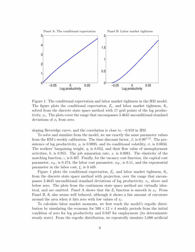
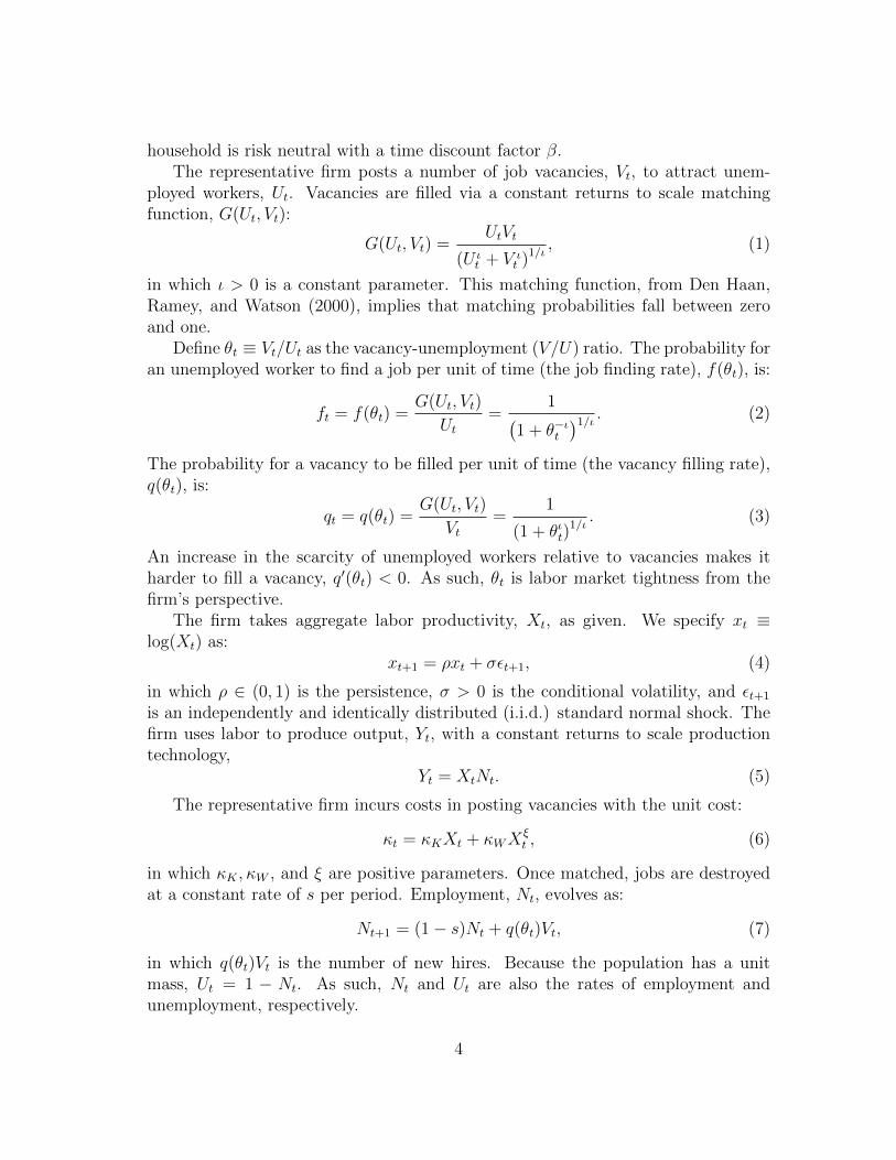
Panel A: The conditional expectation Panel B: Labor market tightness

−0.05 0 0.050

1

2

3

4

5

Log productivity−0.05 0 0.05

0

0.5

1

1.5

2

Log productivity

Figure 1: The conditional expectation and labor market tightness in the HM model.The figure plots the conditional expectation, Et, and labor market tightness, θt,solved from the discrete state space method with 17 grid points of the log produc-tivity, xt. The plots cover the range that encompasses 3.4645 unconditional standarddeviations of xt from zero.

sloping Beveridge curve, and the correlation is close to −0.919 in HM.To solve and simulate from the model, we use exactly the same parameter values

from the HM’s weekly calibration. The time discount factor, β, is 0.991/12. The per-sistence of log productivity, ρ, is 0.9895, and its conditional volatility, σ, is 0.0034.The workers’ bargaining weight, η, is 0.052, and their flow value of unemploymentactivities, b, is 0.955. The job separation rate, s, is 0.0081. The elasticity of thematching function, ι, is 0.407. Finally, for the vacancy cost function, the capital costparameter, κK , is 0.474, the labor cost parameter, κW , is 0.11, and the exponentialparameter in the labor cost, ξ, is 0.449.

Figure 1 plots the conditional expectation, Et, and labor market tightness, θt,from the discrete state space method with projection, over the range that encom-passes 3.4645 unconditional standard deviations of log productivity, xt, above andbelow zero. The plots from the continuous state space method are virtually iden-tical, and are omitted. Panel A shows that the Et function is smooth in xt. FromPanel B, θt also seems well behaved, although it shows a fair amount of curvaturearound the area when it hits zero with low values of xt.

To calculate labor market moments, we first reach the model’s ergodic distri-bution by simulating the economy for 500 × 12 × 4 weekly periods from the initialcondition of zero for log productivity and 0.947 for employment (its deterministicsteady state). From the ergodic distribution, we repeatedly simulate 5,000 artificial

8

samples, each with 648 × 4 weekly periods. We take the quarterly averages of theweekly unemployment, vacancy, and labor productivity to obtain 216 quarterly ob-servations, matching HM’s sample length. We then calculate the model momentsfor each artificial sample, and report the cross-simulation averages.

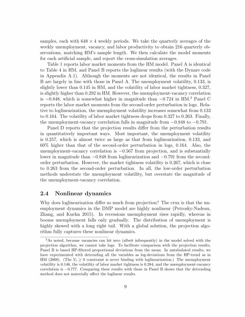
Table 1 reports labor market moments from the HM model. Panel A is identicalto Table 4 in HM, and Panel B reports the loglinear results (with the Dynare codein Appendix A.1). Although the moments are not identical, the results in PanelB are largely in line with those in Panel A. The unemployment volatility, 0.133, isslightly lower than 0.145 in HM, and the volatility of labor market tightness, 0.327,is slightly higher than 0.292 in HM. However, the unemployment-vacancy correlationis −0.848, which is somewhat higher in magnitude than −0.724 in HM.2 Panel Creports the labor market moments from the second-order perturbation in logs. Rela-tive to loglinearization, the unemployment volatility increases somewhat from 0.133to 0.164. The volatility of labor market tightness drops from 0.327 to 0.263. Finally,the unemployment-vacancy correlation falls in magnitude from −0.848 to −0.791.

Panel D reports that the projection results differ from the perturbation resultsin quantitatively important ways. Most important, the unemployment volatilityis 0.257, which is almost twice as large as that from loglinearization, 0.133, and60% higher than that of the second-order perturbation in logs, 0.164. Also, theunemployment-vacancy correlation is −0.567 from projection, and is substantiallylower in magnitude than −0.848 from loglinearization and −0.791 from the second-order perturbation. However, the market tightness volatility is 0.267, which is closeto 0.263 from the second-order perturbation. In all, the low-order perturbationmethods understate the unemployment volatility, but overstate the magnitude ofthe unemployment-vacancy correlation.

2.4 Nonlinear dynamics

Why does loglinearization differ so much from projection? The crux is that the un-employment dynamics in the DMP model are highly nonlinear (Petrosky-Nadeau,Zhang, and Kuehn 2015). In recessions unemployment rises rapidly, whereas inbooms unemployment falls only gradually. The distribution of unemployment ishighly skewed with a long right tail. With a global solution, the projection algo-rithm fully captures these nonlinear dynamics.

2As noted, because vacancies can hit zero (albeit infrequently) in the model solved with theprojection algorithm, we cannot take logs. To facilitate comparison with the projection results,Panel B is based HP-filtered proportional deviations from the mean. In untabulated results, wehave experimented with detrending all the variables as log-deviations from the HP-trend as inHM (2008). (The Vt ≥ 0 constraint is never binding with loglinearization.) The unemploymentvolatility is 0.146, the volatility of labor market tightness is 0.284, and the unemployment-vacancycorrelation is −0.777. Comparing these results with those in Panel B shows that the detrendingmethod does not materially affect the loglinear results.

9

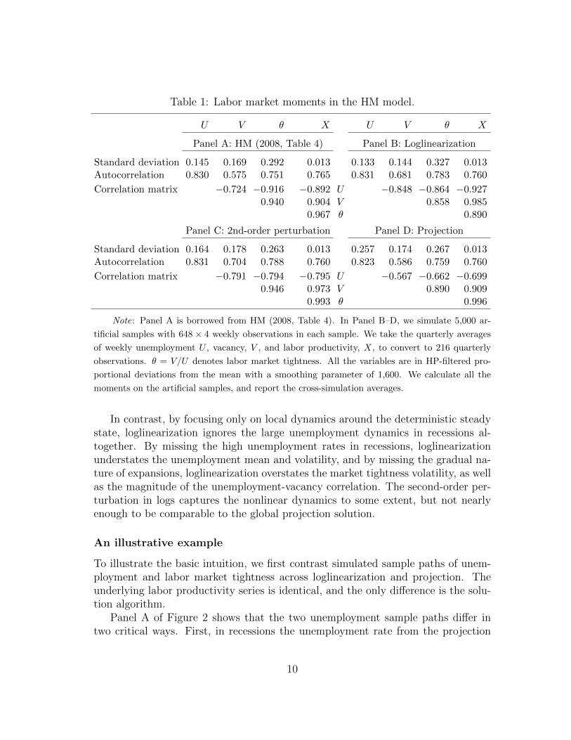
Table 1: Labor market moments in the HM model.

U V θ X U V θ X

Panel A: HM (2008, Table 4) Panel B: Loglinearization

Standard deviation 0.145 0.169 0.292 0.013 0.133 0.144 0.327 0.013Autocorrelation 0.830 0.575 0.751 0.765 0.831 0.681 0.783 0.760

Correlation matrix −0.724 −0.916 −0.892 U −0.848 −0.864 −0.9270.940 0.904 V 0.858 0.985

0.967 θ 0.890

Panel C: 2nd-order perturbation Panel D: Projection

Standard deviation 0.164 0.178 0.263 0.013 0.257 0.174 0.267 0.013Autocorrelation 0.831 0.704 0.788 0.760 0.823 0.586 0.759 0.760

Correlation matrix −0.791 −0.794 −0.795 U −0.567 −0.662 −0.6990.946 0.973 V 0.890 0.909

0.993 θ 0.996

Note: Panel A is borrowed from HM (2008, Table 4). In Panel B–D, we simulate 5,000 ar-

tificial samples with 648 × 4 weekly observations in each sample. We take the quarterly averages

of weekly unemployment U , vacancy, V , and labor productivity, X, to convert to 216 quarterly

observations. θ = V/U denotes labor market tightness. All the variables are in HP-filtered pro-

portional deviations from the mean with a smoothing parameter of 1,600. We calculate all the

moments on the artificial samples, and report the cross-simulation averages.

In contrast, by focusing only on local dynamics around the deterministic steadystate, loglinearization ignores the large unemployment dynamics in recessions al-together. By missing the high unemployment rates in recessions, loglinearizationunderstates the unemployment mean and volatility, and by missing the gradual na-ture of expansions, loglinearization overstates the market tightness volatility, as wellas the magnitude of the unemployment-vacancy correlation. The second-order per-turbation in logs captures the nonlinear dynamics to some extent, but not nearlyenough to be comparable to the global projection solution.

An illustrative example

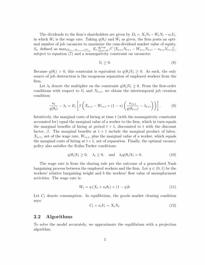
To illustrate the basic intuition, we first contrast simulated sample paths of unem-ployment and labor market tightness across loglinearization and projection. Theunderlying labor productivity series is identical, and the only difference is the solu-tion algorithm.

Panel A of Figure 2 shows that the two unemployment sample paths differ intwo critical ways. First, in recessions the unemployment rate from the projection

10

Panel A: Unemployment Panel B: Labor market tightness

1000 2000 3000 4000 50000

0.05

0.1

0.15

0.2

0.25

1000 2000 3000 4000 50000

1

2

3

4

Figure 2: An illustrative example of simulated sample paths of unemployment andlabor market tightness with identical productivity shocks, projection versus loglin-earization in the HM model. This figure plots the series for unemployment, Ut, andfor labor market tightness, θt, with 5,000 weekly periods. The blue solid line isfrom the projection algorithm, and the red broken line from loglinearization. Theunderlying log productivity process, xt, is fixed across the two algorithms.

algorithm can spike up to more than 10% (the blue solid line), but no such spikesare visible from the loglinearization path (the red broken line). For instance, in the1379th weekly period, the unemployment rate from projection spikes up to 28.64%,whereas the corresponding unemployment rate from loglinearization is only 8.67%.Second, in booms the unemployment rate from projection is often higher than thatfrom loglinearization. In particular, in the 4025th week the unemployment rate fromprojection reaches a low level of 3.44%. However, the corresponding unemploymentrate from loglinearization is even lower, 1.47%.

Relatedly, Panel B shows that the two market tightness series differ mostly inbooms. (The two corresponding vacancy series are largely similar, and are omittedto save space.) In particular, the projection-based market tightness in the 4025thweek is 1.54, which is only 40% of that from loglinearization, 3.83. The market tight-ness from loglinearization often spikes up in booms, but the spikes from projectionare much less visible.

Ergodic distribution

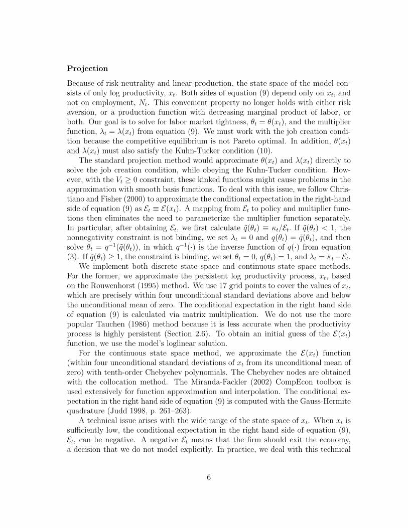
Figure 3 plots unemployment, Ut, vacancy, Vt, and the labor market tightness, θt,against the log productivity, xt, using one million weekly periods simulated from the

11

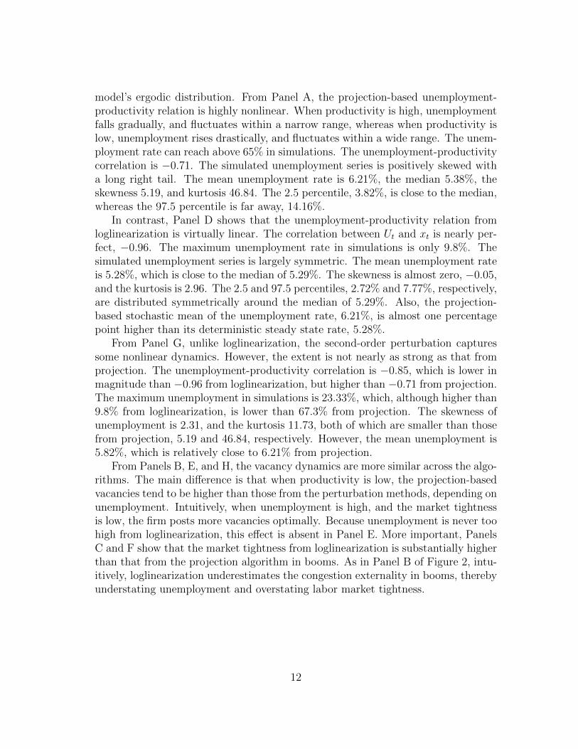
model’s ergodic distribution. From Panel A, the projection-based unemployment-productivity relation is highly nonlinear. When productivity is high, unemploymentfalls gradually, and fluctuates within a narrow range, whereas when productivity islow, unemployment rises drastically, and fluctuates within a wide range. The unem-ployment rate can reach above 65% in simulations. The unemployment-productivitycorrelation is −0.71. The simulated unemployment series is positively skewed witha long right tail. The mean unemployment rate is 6.21%, the median 5.38%, theskewness 5.19, and kurtosis 46.84. The 2.5 percentile, 3.82%, is close to the median,whereas the 97.5 percentile is far away, 14.16%.

In contrast, Panel D shows that the unemployment-productivity relation fromloglinearization is virtually linear. The correlation between Ut and xt is nearly per-fect, −0.96. The maximum unemployment rate in simulations is only 9.8%. Thesimulated unemployment series is largely symmetric. The mean unemployment rateis 5.28%, which is close to the median of 5.29%. The skewness is almost zero, −0.05,and the kurtosis is 2.96. The 2.5 and 97.5 percentiles, 2.72% and 7.77%, respectively,are distributed symmetrically around the median of 5.29%. Also, the projection-based stochastic mean of the unemployment rate, 6.21%, is almost one percentagepoint higher than its deterministic steady state rate, 5.28%.

From Panel G, unlike loglinearization, the second-order perturbation capturessome nonlinear dynamics. However, the extent is not nearly as strong as that fromprojection. The unemployment-productivity correlation is −0.85, which is lower inmagnitude than −0.96 from loglinearization, but higher than −0.71 from projection.The maximum unemployment in simulations is 23.33%, which, although higher than9.8% from loglinearization, is lower than 67.3% from projection. The skewness ofunemployment is 2.31, and the kurtosis 11.73, both of which are smaller than thosefrom projection, 5.19 and 46.84, respectively. However, the mean unemployment is5.82%, which is relatively close to 6.21% from projection.

From Panels B, E, and H, the vacancy dynamics are more similar across the algo-rithms. The main difference is that when productivity is low, the projection-basedvacancies tend to be higher than those from the perturbation methods, depending onunemployment. Intuitively, when unemployment is high, and the market tightnessis low, the firm posts more vacancies optimally. Because unemployment is never toohigh from loglinearization, this effect is absent in Panel E. More important, PanelsC and F show that the market tightness from loglinearization is substantially higherthan that from the projection algorithm in booms. As in Panel B of Figure 2, intu-itively, loglinearization underestimates the congestion externality in booms, therebyunderstating unemployment and overstating labor market tightness.

12

Panel A: Projection, Ut-xt Panel B: Projection, Vt-xt Panel C: Projection, θt-xt

Panel D: Loglinearization,Ut-xt

Panel E: Loglinearization,Vt-xt

Panel F: Loglinearization,θt-xt

Panel G: 2nd-orderperturbation, Ut-xt

Panel H: 2nd-orderperturbation, Vt-xt

Panel I: 2nd-orderperturbation, θt-xt

Figure 3: Unemployment, vacancy, and labor market tightness in simulations inthe HM model. From the model’s ergodic distribution based on each algorithm, wesimulate one million weekly periods, and present the scatter plots of unemployment,Ut, vacancy, Vt, and labor market tightness, θt, against log labor productivity, xt.

13

Nonlinear impulse responses

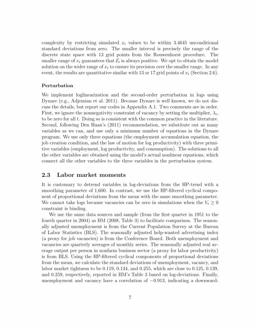
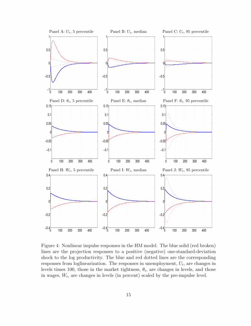
To further illustrate the nonlinear dynamics of the model, we report impulse re-sponses. We consider three different initial points, bad, median, and good economies.The bad economy is the 5 percentile of the model’s bivariate distribution of employ-ment and log productivity with projection, the median economy the 50 percentile,and the good economy the 95 percentile. (Although the job creation condition inequation (9) depends only on the labor productivity, other variables such as con-sumption, unemployment, and output also depend on the current period employ-ment.) The unemployment rates are 10.73%, 5.37%, and 3.97%, and the log pro-ductivity levels are −0.0387, 0, and 0.0383, across the bad, median, and the goodeconomies, respectively. We calculate the responses to a one-standard-deviationshock to the log productivity, both positive and negative, starting from a given ini-tial point. The impulse responses are averaged across 5,000 simulations, each with480 weeks.

Figure 4 reports the impulse responses. Several nonlinear patterns emerge. First,the responses from the projection algorithm are clearly stronger in recessions thanthose in booms. For instance, in response to a negative impulse, the unemploymentrate shoots up by 0.85% in the bad economy (Panel A). In contrast, the responseis only 0.08%, which is an order of magnitude smaller, in the good economy (PanelC). The response in the median economy is 0.19%, which is closer to that in thegood economy than that in the bad economy (Panel B).

Second, and more important, although close in the median economy, the re-sponses in unemployment from loglinearization diverge significantly from the pro-jection responses in recessions and in booms. In particular, the responses from loglin-earization are substantially weaker in the bad economy. The response to a negativeimpulse under loglinearization is 0.15%, which is less than 20% of the projectionresponse, 0.85%. However, in the good economy, the loglinearization responses aresomewhat stronger than the projection responses. The loglinearization response to anegative impulse is 0.16%, which is twice as large as the projection response, 0.08%.Third, the responses in the market tightness are largely similar in the bad and me-dian economies across the two algorithms (Panels D and E). However, the projectionresponses are only about one half of those from loglinearization (Panel F). Intuitively,loglinearization understates the congestion externality and the gradual nature of ex-pansions, but the effect can be fully captured by the projection algorithm.

Finally, wages are endogenously inertial. In the bad economy, in response to anegative impulse, wages drop by only about 0.12% relative to its pre-impulse level inthe projection solution (Panel H). This percentage drop in wages is even lower thanthat in the good economy, 0.18% (Panel J). Relative to projection, loglinearizationunderstates the percentage drop in the bad economy to be 0.08%, but overstatesthat in the good economy to be 0.33%.

14

Panel A: Ut, 5 percentile Panel B: Ut, median Panel C: Ut, 95 percentile

0 100 200 300 400−1

−0.5

0

0.5

1

0 100 200 300 400−1

−0.5

0

0.5

1

0 100 200 300 400−1

−0.5

0

0.5

1

Panel D: θt, 5 percentile Panel E: θt, median Panel F: θt, 95 percentile

0 100 200 300 400

−0.1

−0.05

0

0.05

0.1

0.15

0 100 200 300 400

−0.1

−0.05

0

0.05

0.1

0.15

0 100 200 300 400

−0.1

−0.05

0

0.05

0.1

0.15

Panel H: Wt, 5 percentile Panel I: Wt, median Panel J: Wt, 95 percentile

0 100 200 300 400−0.4

−0.2

0

0.2

0.4

0 100 200 300 400−0.4

−0.2

0

0.2

0.4

0 100 200 300 400−0.4

−0.2

0

0.2

0.4

Figure 4: Nonlinear impulse responses in the HM model. The blue solid (red broken)lines are the projection responses to a positive (negative) one-standard-deviationshock to the log productivity. The blue and red dotted lines are the correspondingresponses from loglinearization. The responses in unemployment, Ut, are changes inlevels times 100, those in the market tightness, θt, are changes in levels, and thosein wages, Wt, are changes in levels (in percent) scaled by the pre-impulse level.

15

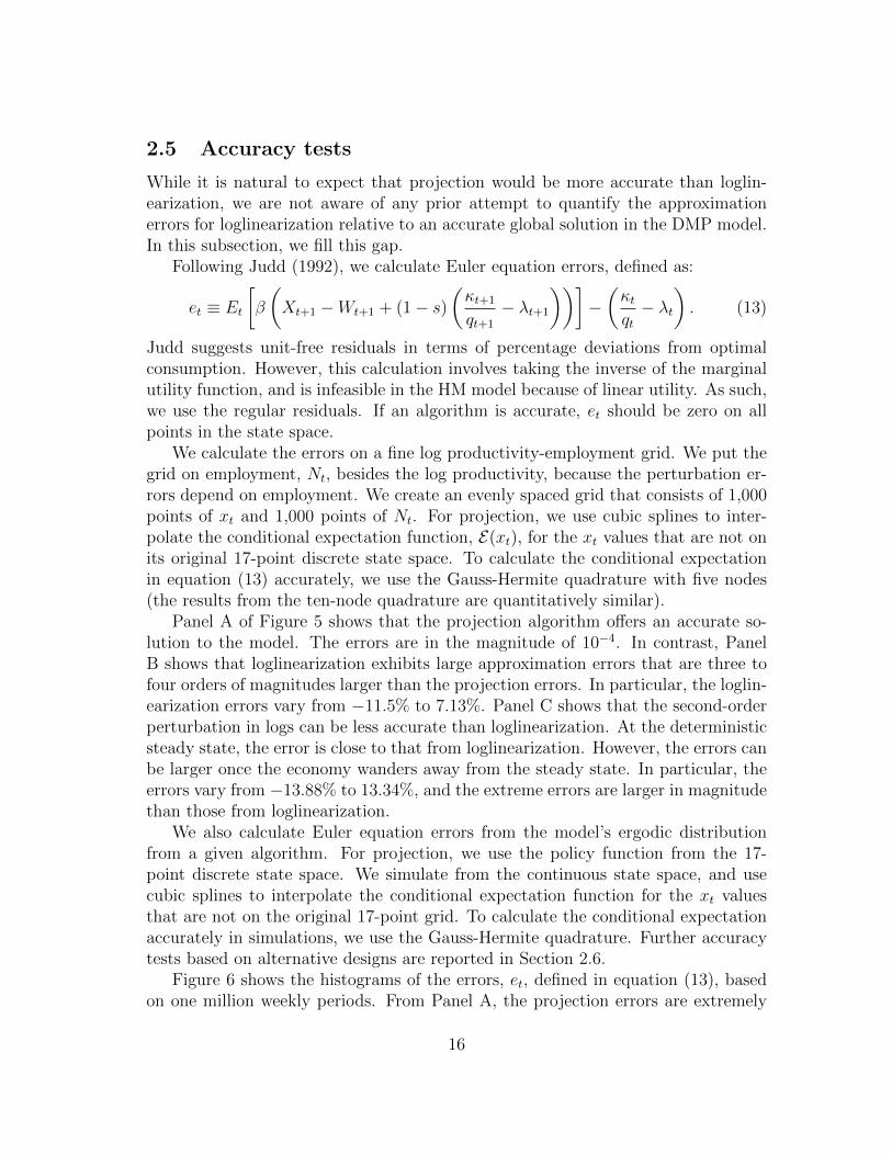
2.5 Accuracy tests

While it is natural to expect that projection would be more accurate than loglin-earization, we are not aware of any prior attempt to quantify the approximationerrors for loglinearization relative to an accurate global solution in the DMP model.In this subsection, we fill this gap.

Following Judd (1992), we calculate Euler equation errors, defined as:

et ≡ Et

[β

(Xt+1 −Wt+1 + (1− s)

(κt+1

qt+1

− λt+1

))]−(κtqt− λt

). (13)

Judd suggests unit-free residuals in terms of percentage deviations from optimalconsumption. However, this calculation involves taking the inverse of the marginalutility function, and is infeasible in the HM model because of linear utility. As such,we use the regular residuals. If an algorithm is accurate, et should be zero on allpoints in the state space.

We calculate the errors on a fine log productivity-employment grid. We put thegrid on employment, Nt, besides the log productivity, because the perturbation er-rors depend on employment. We create an evenly spaced grid that consists of 1,000points of xt and 1,000 points of Nt. For projection, we use cubic splines to inter-polate the conditional expectation function, E(xt), for the xt values that are not onits original 17-point discrete state space. To calculate the conditional expectationin equation (13) accurately, we use the Gauss-Hermite quadrature with five nodes(the results from the ten-node quadrature are quantitatively similar).

Panel A of Figure 5 shows that the projection algorithm offers an accurate so-lution to the model. The errors are in the magnitude of 10−4. In contrast, PanelB shows that loglinearization exhibits large approximation errors that are three tofour orders of magnitudes larger than the projection errors. In particular, the loglin-earization errors vary from −11.5% to 7.13%. Panel C shows that the second-orderperturbation in logs can be less accurate than loglinearization. At the deterministicsteady state, the error is close to that from loglinearization. However, the errors canbe larger once the economy wanders away from the steady state. In particular, theerrors vary from −13.88% to 13.34%, and the extreme errors are larger in magnitudethan those from loglinearization.

We also calculate Euler equation errors from the model’s ergodic distributionfrom a given algorithm. For projection, we use the policy function from the 17-point discrete state space. We simulate from the continuous state space, and usecubic splines to interpolate the conditional expectation function for the xt valuesthat are not on the original 17-point grid. To calculate the conditional expectationaccurately in simulations, we use the Gauss-Hermite quadrature. Further accuracytests based on alternative designs are reported in Section 2.6.

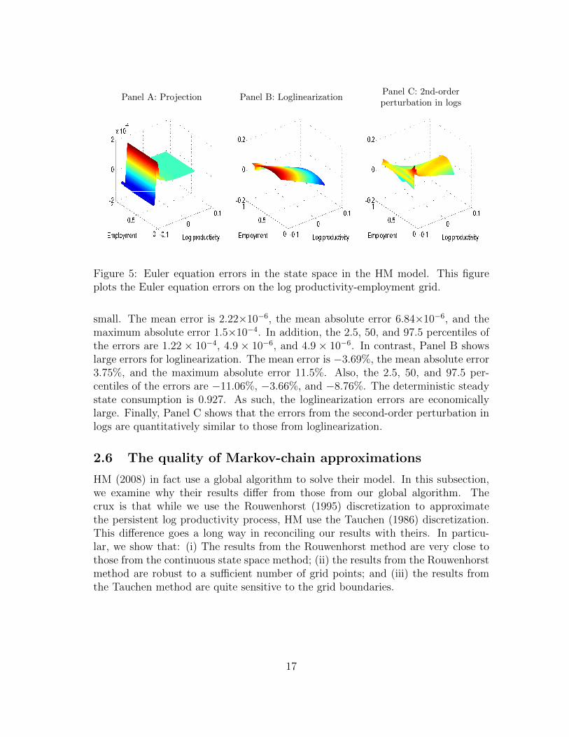
Figure 6 shows the histograms of the errors, et, defined in equation (13), basedon one million weekly periods. From Panel A, the projection errors are extremely

16

Panel A: Projection Panel B: LoglinearizationPanel C: 2nd-orderperturbation in logs

Figure 5: Euler equation errors in the state space in the HM model. This figureplots the Euler equation errors on the log productivity-employment grid.

small. The mean error is 2.22×10−6, the mean absolute error 6.84×10−6, and themaximum absolute error 1.5×10−4. In addition, the 2.5, 50, and 97.5 percentiles ofthe errors are 1.22 × 10−4, 4.9 × 10−6, and 4.9 × 10−6. In contrast, Panel B showslarge errors for loglinearization. The mean error is −3.69%, the mean absolute error3.75%, and the maximum absolute error 11.5%. Also, the 2.5, 50, and 97.5 per-centiles of the errors are −11.06%, −3.66%, and −8.76%. The deterministic steadystate consumption is 0.927. As such, the loglinearization errors are economicallylarge. Finally, Panel C shows that the errors from the second-order perturbation inlogs are quantitatively similar to those from loglinearization.

2.6 The quality of Markov-chain approximations

HM (2008) in fact use a global algorithm to solve their model. In this subsection,we examine why their results differ from those from our global algorithm. Thecrux is that while we use the Rouwenhorst (1995) discretization to approximatethe persistent log productivity process, HM use the Tauchen (1986) discretization.This difference goes a long way in reconciling our results with theirs. In particu-lar, we show that: (i) The results from the Rouwenhorst method are very close tothose from the continuous state space method; (ii) the results from the Rouwenhorstmethod are robust to a sufficient number of grid points; and (iii) the results fromthe Tauchen method are quite sensitive to the grid boundaries.

17

Panel A: Projection Panel B: LoglinearizationPanel C: 2nd-orderperturbation in logs

−2 −1 0 1 2

x 10−4

0

1

2

3

4

5

6x 10

5

Euler equation errors−0.15 −0.1 −0.05 0 0.05

0

1

2

3

4

5

6x 10

4

Euler equation errors−0.15 −0.1 −0.05 0 0.05

0

1

2

3

4

5

6x 10

4

Euler equation errors

Figure 6: Euler equation errors in simulations in the HM model. We simulateone million weekly periods from the model’s ergodic distribution based on eachalgorithm, and plot the histograms for the Euler residuals. The underlying logproductivity series, xt, is identical across the three panels, which differ only in thealgorithm.

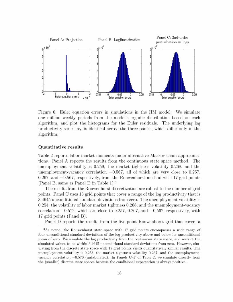
Quantitative results

Table 2 reports labor market moments under alternative Markov-chain approxima-tions. Panel A reports the results from the continuous state space method. Theunemployment volatility is 0.259, the market tightness volatility 0.268, and theunemployment-vacancy correlation −0.567, all of which are very close to 0.257,0.267, and −0.567, respectively, from the Rouwenhorst method with 17 grid points(Panel B, same as Panel D in Table 1).3

The results from the Rouwenhorst discretization are robust to the number of gridpoints. Panel C uses 13 grid points that cover a range of the log productivity that is3.4645 unconditional standard deviations from zero. The unemployment volatility is0.254, the volatility of labor market tightness 0.268, and the unemployment-vacancycorrelation −0.572, which are close to 0.257, 0.267, and −0.567, respectively, with17 grid points (Panel B).

Panel D reports the results from the five-point Rouwenhorst grid that covers a

3As noted, the Rouwenhorst state space with 17 grid points encompasses a wide range offour unconditional standard deviations of the log productivity above and below its unconditionalmean of zero. We simulate the log productivity from the continuous state space, and restrict thesimulated values to be within 3.4645 unconditional standard deviations from zero. However, sim-ulating from the discrete state space with 17 grid points yields quantitatively similar results. Theunemployment volatility is 0.253, the market tightness volatility 0.267, and the unemployment-vacancy correlation −0.570 (untabulated). In Panels C–F of Table 2, we simulate directly fromthe (smaller) discrete state spaces because the conditional expectation is always positive.

18

Table 2: Labor market moments under alternative approximations to the persistentproductivity process.

U V θ X U V θ X

Panel A: Continuous state space Panel B: Rouwenhorst, nx = 17

Standard deviation 0.259 0.175 0.268 0.013 0.257 0.174 0.267 0.013Autocorrelation 0.823 0.586 0.760 0.760 0.823 0.586 0.759 0.760

Correlation matrix −0.567 −0.662 −0.698 U −0.567 −0.662 −0.6990.890 0.909 V 0.890 0.909

0.996 θ 0.996

Panel C: Rouwenhorst, nx = 13 Panel D: Rouwenhorst, nx = 5

Standard deviation 0.254 0.175 0.268 0.013 0.219 0.172 0.267 0.013Autocorrelation 0.827 0.583 0.759 0.760 0.830 0.581 0.760 0.760

Correlation matrix −0.572 −0.669 −0.704 U −0.608 −0.716 −0.7440.891 0.908 V 0.901 0.914

0.997 θ 0.998

Panel E: Tauchen, m = 2 Panel F: Tauchen, m = 3.4645

Standard deviation 0.154 0.149 0.246 0.013 0.299 0.192 0.286 0.014Autocorrelation 0.813 0.582 0.749 0.747 0.825 0.580 0.759 0.760

Correlation matrix −0.697 −0.825 −0.842 U −0.535 −0.625 −0.6690.930 0.936 V 0.876 0.899

0.997 θ 0.995

Note: Results are averaged across 5,000 samples from each approximation with the projection

algorithm. nx is the number of grid points for the log productivity, xt, in the Rouwenhorst

discretization. When implementing the Tauchen discretization of xt, we use 35 grid points, but

vary the boundaries of the grid in terms of the number of unconditional standard deviations,

denoted m, from the unconditional mean of zero. The simulation design is identical to Table 1.

19

range of two unconditional standard deviations above and below zero. We choosethis range to be comparable with the HM implementation of the Tauchen methodthat also covers a range of two standard deviations from zero. Even with only fivegrid points, the unemployment volatility is 0.219, which is not far from 0.257 with 17grid points. The market tightness volatility is 0.267, which is identical to that fromthe larger grid. Finally, the unemployment-vacancy correlation is −0.608, which isnot far from −0.567 from the 17-point grid.

Panels E and F show that the results from the Tauchen discretization are quitesensitive to the range of the grid chosen. Unlike the Rouwenhorst procedure, inwhich the number of grid points automatically determines the range of the grid, theTauchen method allows a separate parameter to pin down the grid range, regardlessof the number of grid points. We always use 35 grid points as in HM, but experimentwith two different ranges that cover two and 3.4645 unconditional standard devia-tions of the log productivity from zero. From Panel E, with the smaller range as inHM, the results from the Tauchen method are largely in line with those reported intheir Table 4 (see Panel A of our Table 1). The unemployment volatility is 0.154,the market tightness volatility 0.246, and the unemployment-vacancy correlation−0.697, which are (relatively) close to 0.145, 0.292, and −0.724, respectively, in HM.

Panel F shows that enlarging the range of the Tauchen grid raises the unemploy-ment volatility, but dampens the unemployment-vacancy correlation. When therange increases from two to 3.4645 unconditional standard deviations from zero, theunemployment volatility rises from 0.154 to 0.299, and the unemployment-vacancycorrelation falls in magnitude from −0.697 to −0.535. The market tightness volatil-ity also increases somewhat from 0.246 to 0.286. The only difference between PanelsE and F is the range parameter of the Tauchen grid. As such, these results castdoubt on the Tauchen method, but lend support to the Rouwenhorst method inapproximating highly persistent autoregressive processes.4

Euler equation errors

Figure 7 reports the Euler residuals from the model’s ergodic distribution based ona given approximation procedure of the continuous log productivity process, xt. InPanel A, we use the policy function approximated with the ten-order Chebychevpolynomials, which are in turn used to interpolate the policy rule on the simulatedxt values that are not directly on the original Chebychev nodes. The Euler residualsare largely comparable with those from the discrete Rouwenhorst method with 17grid points. In particular, the mean error, the mean absolute error, and the maxi-

4Kopecky and Suen (2010) also note that the performance of the Tauchen (1986) method isextremely sensitive to the choice of the free parameter that determines the range of the discretestate space. Their results are based on the stochastic growth model. We echo their conclusion inthe context of the DMP model.

20

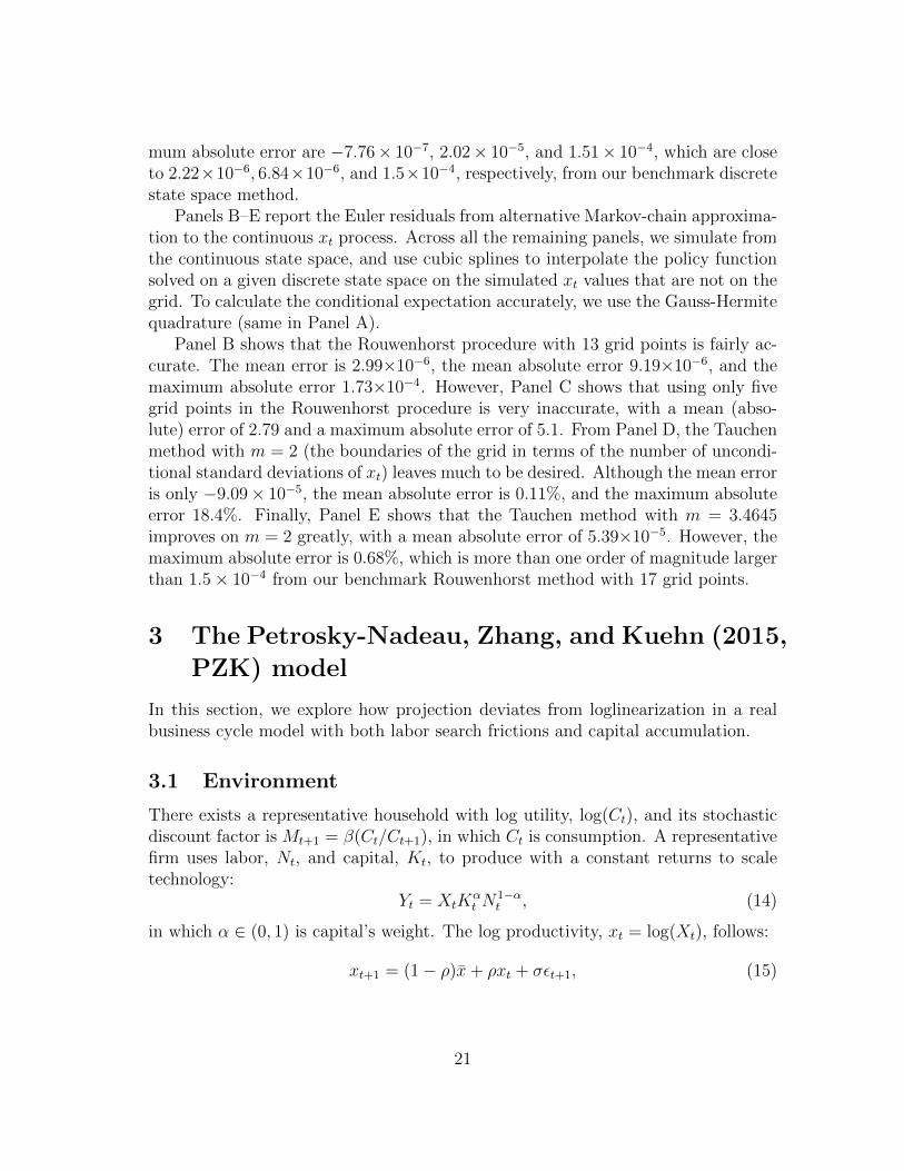
mum absolute error are −7.76× 10−7, 2.02× 10−5, and 1.51× 10−4, which are closeto 2.22×10−6, 6.84×10−6, and 1.5×10−4, respectively, from our benchmark discretestate space method.

Panels B–E report the Euler residuals from alternative Markov-chain approxima-tion to the continuous xt process. Across all the remaining panels, we simulate fromthe continuous state space, and use cubic splines to interpolate the policy functionsolved on a given discrete state space on the simulated xt values that are not on thegrid. To calculate the conditional expectation accurately, we use the Gauss-Hermitequadrature (same in Panel A).

Panel B shows that the Rouwenhorst procedure with 13 grid points is fairly ac-curate. The mean error is 2.99×10−6, the mean absolute error 9.19×10−6, and themaximum absolute error 1.73×10−4. However, Panel C shows that using only fivegrid points in the Rouwenhorst procedure is very inaccurate, with a mean (abso-lute) error of 2.79 and a maximum absolute error of 5.1. From Panel D, the Tauchenmethod with m = 2 (the boundaries of the grid in terms of the number of uncondi-tional standard deviations of xt) leaves much to be desired. Although the mean erroris only −9.09× 10−5, the mean absolute error is 0.11%, and the maximum absoluteerror 18.4%. Finally, Panel E shows that the Tauchen method with m = 3.4645improves on m = 2 greatly, with a mean absolute error of 5.39×10−5. However, themaximum absolute error is 0.68%, which is more than one order of magnitude largerthan 1.5× 10−4 from our benchmark Rouwenhorst method with 17 grid points.

3 The Petrosky-Nadeau, Zhang, and Kuehn (2015,

PZK) model

In this section, we explore how projection deviates from loglinearization in a realbusiness cycle model with both labor search frictions and capital accumulation.

3.1 Environment

There exists a representative household with log utility, log(Ct), and its stochasticdiscount factor is Mt+1 = β(Ct/Ct+1), in which Ct is consumption. A representativefirm uses labor, Nt, and capital, Kt, to produce with a constant returns to scaletechnology:

Yt = XtKαt N

1−αt , (14)

in which α ∈ (0, 1) is capital’s weight. The log productivity, xt = log(Xt), follows:

xt+1 = (1− ρ)x+ ρxt + σεt+1, (15)

21

Panel A: Continuous statespace

Panel B: Rouwenhorst,nx = 13

Panel C: Rouwenhorst,nx = 5

−2 −1 0 1 2

x 10−4

0

0.5

1

1.5

2x 10

5

Euler equation errors−2 −1 0 1 2

x 10−4

0

2

4

6

8x 10

5

Euler equation errors0 2 4 6

0

1

2

3

4

5

6x 10

4

Euler equation errors

Panel D: Tauchen, m = 2Panel E: Tauchen,

m = 3.4645

−0.2 −0.1 0 0.1 0.20

2

4

6

8

10x 10

5

Euler equation errors−0.01 −0.005 0 0.005 0.01

0

2

4

6

8

10x 10

5

Euler equation errors

Figure 7: Further results on Euler equation errors in simulations in the HM model.We simulate one million weekly periods from the model’s ergodic distribution basedon each approximation of the continuous log productivity process, and plot thehistograms for the Euler residuals. The underlying log productivity series, xt, isidentical across all the panels (and is the same series as in Figure 6). All the panelsuse the projection algorithm, but differ in the approximation procedure of xt.

22

in which x is the unconditional mean of xt. We rescale x to ensure the averagemarginal product of labor to be unity in simulations to facilitate interpretation ofparameter values.

The firm posts vacancies, Vt, to attract unemployed workers, Ut. The matchingfunction is given by equation (1). We continue to impose the nonnegativity con-straint on vacancies. When posting vacancies, the firm incurs the constant unit costof κ. The firm also invests, and occurs adjustment costs when doing so. Capitalaccumulates as:

Kt+1 = (1− δ)Kt + Φ(It, Kt), (16)

in which δ is the capital depreciation rate, and It is investment. The installationfunction is:

Φ(It, Kt) =

[a1 +

a21− 1/ν

(ItKt

)1−1/ν]Kt, (17)

in which ν > 0 is the supply elasticity of capital. We set a1 = δ/(1−ν) and a2 = δ1/ν

to ensure no adjustment costs in the deterministic steady state (Jermann 1998).The equilibrium wage, Wt, follows:

Wt = η

[(1− α)

YtNt

+ κθt

]+ (1− η)b, (18)

in which the marginal product of labor is given by (1− α)Yt/Nt. The dividends tothe firm’s shareholders are given by Dt ≡ Yt−WtNt−κVt− It. Taking q(θt) and Wt

as given, the firm chooses an optimal number of vacancies and optimal investmentto maximize the present value of all future dividends, subject to equations (7) and(16), as well as the vacancy nonnegativity constraint. In equilibrium, the marketclearing condition says:

Ct + It + κVt = Yt. (19)

Optimality conditions include the intertemporal job creation condition:

κ

q(θt)− λt = Et

[Mt+1

((1− α)

Yt+1

Nt+1

−Wt+1 + (1− s)(

κ

q(θt+1)− λt+1

))], (20)

and the investment Euler equation:

1

a2

(ItKt

)1/ν

= Et

[Mt+1

(αYt+1

Kt+1

+1

a2

(It+1

Kt+1

)1/ν

(1− δ + a1) +1

ν − 1

It+1

Kt+1

)],

(21)as well as the Kuhn-Tucker conditions in equation (10).5

5Under our benchmark calibration (Section 3.3), the vacancy nonnegativity constraint is neverbinding. Intuitively, capital provides a buffer to negative shocks so that vacancy does not fall tozero. As such, zero vacancies are specific to the Hagedorn-Manovskii (2008) model with linearutility and no capital in production.

23

3.2 Algorithms

Because of its disaster dynamics (PZK 2015), the projection algorithm for the PZKmodel is challenging. Also, risk aversion and nonlinear production function implythat the model has three separate state variables, employment, Nt, capital, Kt, andlog productivity, xt. We solve for the optimal vacancy function, V (Nt, Kt, xt), themultiplier function, λ(Nt, Kt, xt), and the optimal investment function, I(Nt, Kt, xt),from the intertemporal job creation condition in equation (20) and the investmentEuler equation (21). The policy functions must also satisfy the Kuhn-Tucker con-ditions in equation (10). Because optimal investment is always positive, we approx-imate I(Nt, Kt, xt) directly. The positive investment is a result of the installationfunction in equation (17). In particular, when investment goes to zero, the marginalbenefit of investment, ∂Φ(It, Kt)/∂It = a2(It/Kt)

−1/ν , goes to infinity. Finally, toimpose the vacancy nonnegativity constraint, we continue to parameterize the condi-tional expectation in the right hand side of equation (20), denoted Et ≡ E(Nt, Kt, xt).

Following the recommendation of Fernandez-Villaverde, Rubio-Ramırez, andSchorfheide (2016), we discretize the log productivity, xt, with the Rouwenhorstprocedure with 17 grid points.6 The discrete state space simplifies the computa-tion of conditional expectations to matrix multiplication, and alleviates the curse ofdimensionality.

We approximate I(Nt, Kt, xt) and E(Nt, Kt, xt) on each grid point of xt. Our pri-mary concern is with accuracy, not running time. We use the finite element methodwith cubic splines on 100 nodes on the employment space, Nt ∈ [0.225, 0.975], and100 nodes on the capital space, Kt ∈ [10, 42.5]. We take the tensor product of Nt andKt for each grid point of xt. We use the Miranda-Fackler CompEcon toolbox exten-sively for function approximation and interpolation. With two functional equationson the 17-point xt-grid, the 100-point Nt-grid, and the 100-point Kt-grid, we need tosolve a system of 340,000 nonlinear equations. The traditional Newton-style meth-ods are infeasible for such a large system. Following the recommendation of Judd,Maliar, Maliar, and Valero (2014), we use derivative-free fixed-point iteration witha damping parameter of 0.025. The convergence criterion is set to be 10−10 for themaximum absolute value of the Euler equation errors across the nonlinear equations.

To obtain a good initial guess, we proceed sequentially. We first use the loglinearsolution as the initial guess on a small grid with only five points for employment andfor capital. The initial grid only covers a small interval of employment from 0.9 to0.975 and a small interval of capital from 30 to 40. We always use the 17-point gridfor the log productivity. Upon convergence, we use the projection solution as the newinitial guess. We then gradually expand the employment and capital grids by adding

6Fernandez-Villaverde, Rubio-Ramırez, and Schorfheide (2016, p. 78) write that “discretizationof state variables such as the productivity shock is more often than not an excellent strategy to dealwith multidimensional problems: simple, transparent, and not too burdensome computationally.”

24

Panel A: The lowest xt Panel B: The median xt Panel C: The highest xt

1020

3040

0.5

1−5

0

5

CapitalEmployment 1020

3040

0.5

1−5

0

5

CapitalEmployment 1020

3040

0.5

1−5

0

5

CapitalEmployment

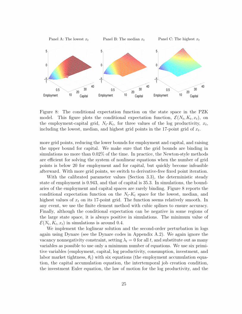
Figure 8: The conditional expectation function on the state space in the PZKmodel. This figure plots the conditional expectation function, E(Nt, Kt, xt), onthe employment-capital grid, Nt-Kt, for three values of the log productivity, xt,including the lowest, median, and highest grid points in the 17-point grid of xt.

more grid points, reducing the lower bounds for employment and capital, and raisingthe upper bound for capital. We make sure that the grid bounds are binding insimulations no more than 0.02% of the time. In practice, the Newton-style methodsare efficient for solving the system of nonlinear equations when the number of gridpoints is below 20 for employment and for capital, but quickly become infeasibleafterward. With more grid points, we switch to derivative-free fixed point iteration.

With the calibrated parameter values (Section 3.3), the deterministic steadystate of employment is 0.943, and that of capital is 35.3. In simulations, the bound-aries of the employment and capital spaces are rarely binding. Figure 8 reports theconditional expectation function on the Nt-Kt space for the lowest, median, andhighest values of xt on its 17-point grid. The function seems relatively smooth. Inany event, we use the finite element method with cubic splines to ensure accuracy.Finally, although the conditional expectation can be negative in some regions ofthe large state space, it is always positive in simulations. The minimum value ofE(Nt, Kt, xt) in simulations is around 0.4.

We implement the loglinear solution and the second-order perturbation in logsagain using Dynare (see the Dynare codes in Appendix A.2). We again ignore thevacancy nonnegativity constraint, setting λt = 0 for all t, and substitute out as manyvariables as possible to use only a minimum number of equations. We use six primi-tive variables (employment, capital, log productivity, consumption, investment, andlabor market tightness, θt) with six equations (the employment accumulation equa-tion, the capital accumulation equation, the intertemporal job creation condition,the investment Euler equation, the law of motion for the log productivity, and the

25

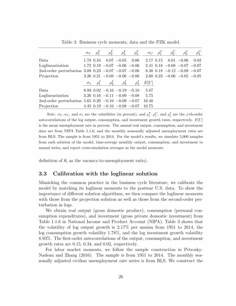
Table 3: Business cycle moments, data and the PZK model.

σY ρY1 ρY2 ρY3 ρY4 σC ρC1 ρC2 ρC3 ρC4

Data 1.78 0.34 0.07 −0.05 0.06 2.17 0.15 0.01 −0.06 0.02Loglinearization 1.72 0.19 −0.07 −0.06 −0.06 2.41 0.18 −0.08 −0.07 −0.072nd-order perturbation 3.08 0.23 −0.07 −0.07 −0.06 8.38 0.18 −0.12 −0.09 −0.07Projection 3.26 0.21 −0.08 −0.06 −0.06 2.60 0.23 −0.06 −0.05 −0.05

σI ρI1 ρI2 ρI3 ρI4 E[U ]

Data 8.93 0.02 −0.16 −0.19 −0.10 5.87Loglinearization 3.26 0.16 −0.11 −0.09 −0.08 5.752nd-order perturbation 5.65 0.20 −0.10 −0.09 −0.07 16.40Projection 4.45 0.19 −0.10 −0.08 −0.07 10.75

Note: σY , σC , and σI are the volatilities (in percent), and ρYj , ρCj , and ρIj are the j-th-order

autocorrelations of the log output, consumption, and investment growth rates, respectively. E[U ]

is the mean unemployment rate in percent. The annual real output, consumption, and investment

data are from NIPA Table 1.1.6, and the monthly seasonally adjusted unemployment rates are

from BLS. The sample is from 1951 to 2014. For the model’s results, we simulate 5,000 samples

from each solution of the model, time-average monthly output, consumption, and investment to

annual series, and report cross-simulation averages as the model moments.

definition of θt as the vacancy-to-unemployment ratio).

3.3 Calibration with the loglinear solution

Mimicking the common practice in the business cycle literature, we calibrate themodel by matching its loglinear moments to the postwar U.S. data. To show theimportance of different solution algorithms, we then compare the loglinear momentswith those from the projection solution as well as those from the second-order per-turbation in logs.

We obtain real output (gross domestic product), consumption (personal con-sumption expenditures), and investment (gross private domestic investment) fromTable 1.1.6 in National Income and Product Account (NIPA). Table 3 shows thatthe volatility of log output growth is 2.17% per annum from 1951 to 2014, thelog consumption growth volatility 1.78%, and the log investment growth volatility8.93%. The first-order autocorrelations of the output, consumption, and investmentgrowth rates are 0.15, 0.34, and 0.02, respectively.

For labor market moments, we follow the sample construction in Petrosky-Nadeau and Zhang (2016). The sample is from 1951 to 2014. The monthly sea-sonally adjusted civilian unemployment rate series is from BLS. We construct the

26

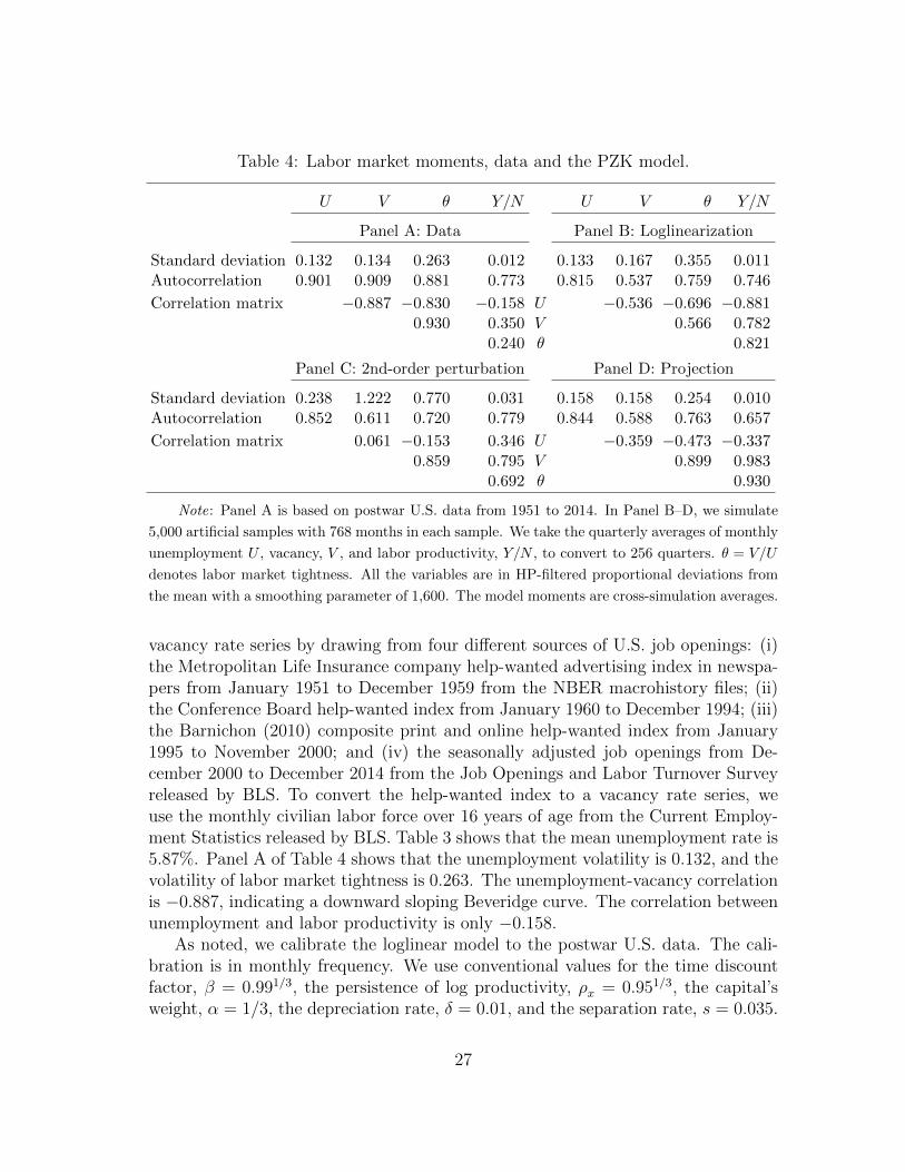
Table 4: Labor market moments, data and the PZK model.

U V θ Y/N U V θ Y/N

Panel A: Data Panel B: Loglinearization

Standard deviation 0.132 0.134 0.263 0.012 0.133 0.167 0.355 0.011Autocorrelation 0.901 0.909 0.881 0.773 0.815 0.537 0.759 0.746

Correlation matrix −0.887 −0.830 −0.158 U −0.536 −0.696 −0.8810.930 0.350 V 0.566 0.782

0.240 θ 0.821

Panel C: 2nd-order perturbation Panel D: Projection

Standard deviation 0.238 1.222 0.770 0.031 0.158 0.158 0.254 0.010Autocorrelation 0.852 0.611 0.720 0.779 0.844 0.588 0.763 0.657

Correlation matrix 0.061 −0.153 0.346 U −0.359 −0.473 −0.3370.859 0.795 V 0.899 0.983

0.692 θ 0.930

Note: Panel A is based on postwar U.S. data from 1951 to 2014. In Panel B–D, we simulate

5,000 artificial samples with 768 months in each sample. We take the quarterly averages of monthly

unemployment U , vacancy, V , and labor productivity, Y/N , to convert to 256 quarters. θ = V/U

denotes labor market tightness. All the variables are in HP-filtered proportional deviations from

the mean with a smoothing parameter of 1,600. The model moments are cross-simulation averages.

vacancy rate series by drawing from four different sources of U.S. job openings: (i)the Metropolitan Life Insurance company help-wanted advertising index in newspa-pers from January 1951 to December 1959 from the NBER macrohistory files; (ii)the Conference Board help-wanted index from January 1960 to December 1994; (iii)the Barnichon (2010) composite print and online help-wanted index from January1995 to November 2000; and (iv) the seasonally adjusted job openings from De-cember 2000 to December 2014 from the Job Openings and Labor Turnover Surveyreleased by BLS. To convert the help-wanted index to a vacancy rate series, weuse the monthly civilian labor force over 16 years of age from the Current Employ-ment Statistics released by BLS. Table 3 shows that the mean unemployment rate is5.87%. Panel A of Table 4 shows that the unemployment volatility is 0.132, and thevolatility of labor market tightness is 0.263. The unemployment-vacancy correlationis −0.887, indicating a downward sloping Beveridge curve. The correlation betweenunemployment and labor productivity is only −0.158.

As noted, we calibrate the loglinear model to the postwar U.S. data. The cali-bration is in monthly frequency. We use conventional values for the time discountfactor, β = 0.991/3, the persistence of log productivity, ρx = 0.951/3, the capital’sweight, α = 1/3, the depreciation rate, δ = 0.01, and the separation rate, s = 0.035.

27

The elasticity of the matching function, ι, is 1.25, which is close to that in Den Haan,Ramey, and Watson (2000). Following Gertler and Trigari (2009), we choose theconditional volatility of the log productivity, σ, to match the output growth volatilityin the data. This procedure yields σ = 0.0065, which implies an output volatility of2.41% per annum in the model, relative to 2.17% in the data. Following PZK (2015),we choose the elasticity in the installation function, ν = 2, such that the consump-tion growth volatility in the model is 1.72%, which is close to 1.78% in the data. How-ever, the investment growth volatility is only 3.26%, in contrast to 8.93% in the data.

We calibrate the remaining labor market parameters in the spirit of HM (2008).The workers’ bargaining weight, η, is 0.04, the flow value of unemployment activities,b, is 0.95, and the cost of vacancy posting, κ, is 0.45. These values imply an averageunemployment rate of 5.75% in the model, which is close to 5.87% in the data, andan unemployment volatility of 0.133, which is close to 0.132 in the data. However,the market tightness volatility is 0.355, which is higher than 0.263 in the data. Inaddition, the unemployment-vacancy correlation is −0.536, which is smaller in mag-nitude than −0.887 in the data, and the unemployment-labor productivity correla-tion is −0.881, which is substantially higher than −0.158 in the data. The weaknessof the DMP model in matching correlations in the data is also present in HM.

3.4 Accuracy tests

Before discussing how the projection moments differ from the perturbation mo-ments, we present accuracy tests of different algorithms. The tests show that theprojection algorithm is accurate, loglinearization inaccurate, and the second-orderperturbation wildly incorrect.

Following Judd (1992), we use unit-free residuals in the unit of optimal consump-tion. Combining the stochastic discount factor with log utility, Mt+1 = β(Ct/Ct+1),with equations (20) and (21) yields the unit-free job creation equation errors, de-noted eVt , as:

eVt ≡

κq(θt)− λt

Et

[β

Ct+1

((1− α) Yt+1

Nt+1−Wt+1 + (1− s)

(κ

q(θt+1)− λt+1

))] − Ct /Ct, (22)

as well as the unit-free investment Euler equation errors, denoted eIt , as:

eIt ≡

1a2

(ItKt

)1/νEt

[β

Ct+1

(α Yt+1

Kt+1+ 1

a2

(It+1

Kt+1

)1/ν(1− δ + a1) + 1

ν−1It+1

Kt+1

)] − Ct /Ct. (23)

Because of our large, three-dimensional state space, Nt-Kt-xt, a significant por-tion of the state space is never visited in simulations even with our projection algo-rithm. As such, we focus on the Euler residuals in simulations because only these

28

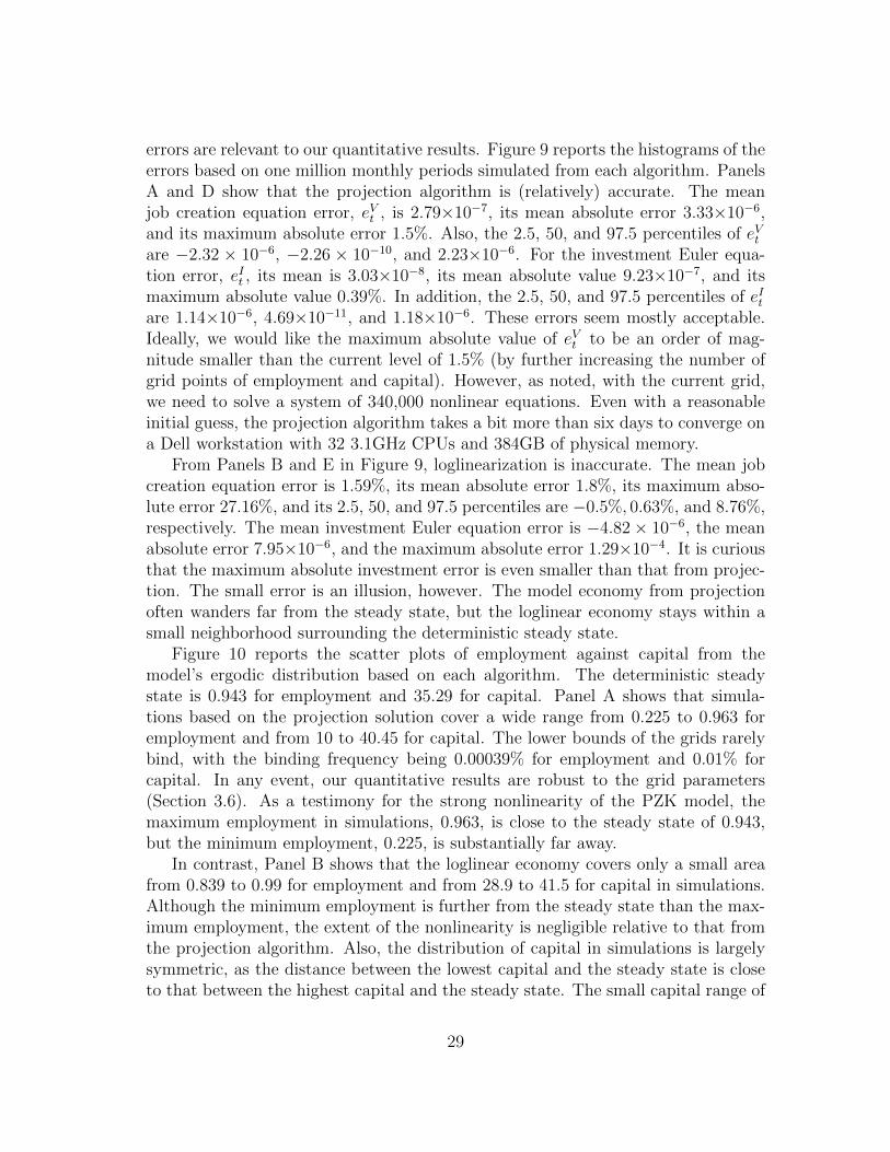
errors are relevant to our quantitative results. Figure 9 reports the histograms of theerrors based on one million monthly periods simulated from each algorithm. PanelsA and D show that the projection algorithm is (relatively) accurate. The meanjob creation equation error, eVt , is 2.79×10−7, its mean absolute error 3.33×10−6,and its maximum absolute error 1.5%. Also, the 2.5, 50, and 97.5 percentiles of eVtare −2.32 × 10−6, −2.26 × 10−10, and 2.23×10−6. For the investment Euler equa-tion error, eIt , its mean is 3.03×10−8, its mean absolute value 9.23×10−7, and itsmaximum absolute value 0.39%. In addition, the 2.5, 50, and 97.5 percentiles of eItare 1.14×10−6, 4.69×10−11, and 1.18×10−6. These errors seem mostly acceptable.Ideally, we would like the maximum absolute value of eVt to be an order of mag-nitude smaller than the current level of 1.5% (by further increasing the number ofgrid points of employment and capital). However, as noted, with the current grid,we need to solve a system of 340,000 nonlinear equations. Even with a reasonableinitial guess, the projection algorithm takes a bit more than six days to converge ona Dell workstation with 32 3.1GHz CPUs and 384GB of physical memory.

From Panels B and E in Figure 9, loglinearization is inaccurate. The mean jobcreation equation error is 1.59%, its mean absolute error 1.8%, its maximum abso-lute error 27.16%, and its 2.5, 50, and 97.5 percentiles are −0.5%, 0.63%, and 8.76%,respectively. The mean investment Euler equation error is −4.82× 10−6, the meanabsolute error 7.95×10−6, and the maximum absolute error 1.29×10−4. It is curiousthat the maximum absolute investment error is even smaller than that from projec-tion. The small error is an illusion, however. The model economy from projectionoften wanders far from the steady state, but the loglinear economy stays within asmall neighborhood surrounding the deterministic steady state.

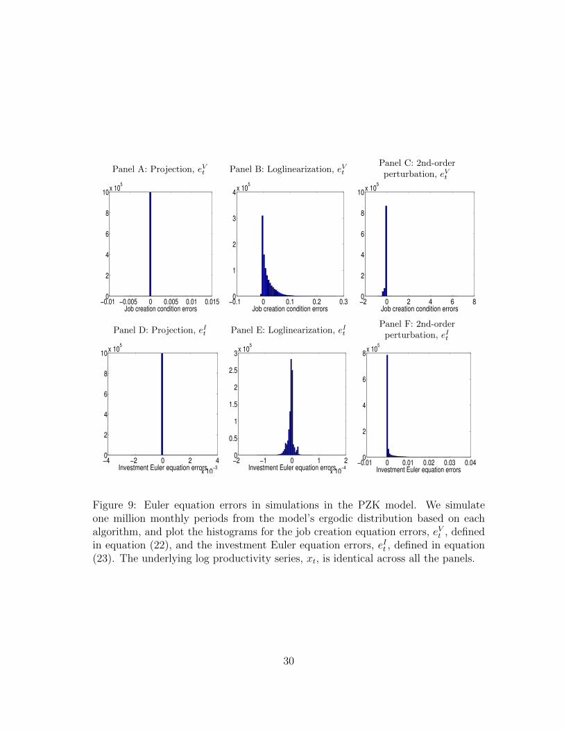
Figure 10 reports the scatter plots of employment against capital from themodel’s ergodic distribution based on each algorithm. The deterministic steadystate is 0.943 for employment and 35.29 for capital. Panel A shows that simula-tions based on the projection solution cover a wide range from 0.225 to 0.963 foremployment and from 10 to 40.45 for capital. The lower bounds of the grids rarelybind, with the binding frequency being 0.00039% for employment and 0.01% forcapital. In any event, our quantitative results are robust to the grid parameters(Section 3.6). As a testimony for the strong nonlinearity of the PZK model, themaximum employment in simulations, 0.963, is close to the steady state of 0.943,but the minimum employment, 0.225, is substantially far away.

In contrast, Panel B shows that the loglinear economy covers only a small areafrom 0.839 to 0.99 for employment and from 28.9 to 41.5 for capital in simulations.Although the minimum employment is further from the steady state than the max-imum employment, the extent of the nonlinearity is negligible relative to that fromthe projection algorithm. Also, the distribution of capital in simulations is largelysymmetric, as the distance between the lowest capital and the steady state is closeto that between the highest capital and the steady state. The small capital range of

29

Panel A: Projection, eVt Panel B: Loglinearization, eVtPanel C: 2nd-orderperturbation, eVt

−0.01 −0.005 0 0.005 0.01 0.0150

2

4

6

8

10x 10

5

Job creation condition errors−0.1 0 0.1 0.2 0.3

0

1

2

3

4x 10

5

Job creation condition errors−2 0 2 4 6 80

2

4

6

8

10x 10

5

Job creation condition errors

Panel D: Projection, eIt Panel E: Loglinearization, eItPanel F: 2nd-order

perturbation, eIt

−4 −2 0 2 4

x 10−3

0

2

4

6

8

10x 10

5

Investment Euler equation errors−2 −1 0 1 2

x 10−4

0

0.5

1

1.5

2

2.5

3x 10

5

Investment Euler equation errors−0.01 0 0.01 0.02 0.03 0.04

0

2

4

6

8x 10

5

Investment Euler equation errors

Figure 9: Euler equation errors in simulations in the PZK model. We simulateone million monthly periods from the model’s ergodic distribution based on eachalgorithm, and plot the histograms for the job creation equation errors, eVt , definedin equation (22), and the investment Euler equation errors, eIt , defined in equation(23). The underlying log productivity series, xt, is identical across all the panels.

30

Panel A: Projection Panel B: LoglinearizationPanel C: 2nd-order

perturbation

Figure 10: The scatter plots of employment versus capital in the PZK model. Wesimulate one million monthly periods from the model’s ergodic distribution basedon each algorithm, and present the scatter plots of employment against capital.

the loglinear economy likely explains why its maximum absolute investment Eulerequation error is smaller than that from the projection algorithm.

Turning our attention to the second-order perturbation in logs, Panels C and Fof Figure 9 show that this algorithm can be dramatically inaccurate, particularly forthe job creation equation. For the errors from this equation, eVt , the mean is −4.06%,the mean absolute value 4.51%, and the maximum absolute value is 654.6%. The2.5, 50, and 97.5 percentiles are −32.23%,−0.23%, and 0.26%, respectively. Theinvestment Euler equation errors, eIt , are more sensible. The mean is 7.56×10−4,the mean absolute value 7.72×10−4, and the maximum absolute value 3.02%. The2.5, 50, and 97.5 percentiles are −6.51× 10−5, 2.25×10−6, and 0.82%, respectively.Also, the correlations of the simulated log productivity, xt, are −0.4 with |eVt |, and−0.45 with |eIt |. As such, the algorithm does particularly poorly in bad times.

The employment-capital scatter plot in Panel C of Figure 10 sheds further lighton why the second-order perturbation performs particularly poorly in approximatingthe job creation equation. The simulated economy covers a wide range of employ-ment from 0.03 to 0.954, and the minimum employment is substantially lower than0.225 from the projection algorithm. Intuitively, the second-order coefficients cal-culated locally around the deterministic steady state induce very large errors, whenthe economy wanders far away from the steady state.

Because of the large Euler residuals from the second-order perturbation in logs,we do not focus on the moments from this algorithm. Briefly, Tables 3 and 4 showthat the volatilities from the second-order perturbation are substantially higher thanthose from projection and loglinearization. Also, the unemployment-vacancy corre-

31

lation is even positive, 0.061, as opposed to negative in both loglinearization andprojection. Because these moments are likely contaminated by large errors, we dis-card them from further discussion.

3.5 How does projection deviate from loglinearization?

Table 3 shows that the volatilities from the projection algorithm are higher thanthose from loglinearization. The output, consumption, and investment growthvolatilities are 3.26%, 2.60%, and 4.45% per annum with projection, which arehigher than 1.72%, 2.41%, and 3.26% with loglinearization, respectively. In con-trast, the autocorrelations of the three growth rates are largely comparable acrossthe two algorithms.

The labor market moments differ even more between projection and loglineariza-tion. The mean unemployment rate is 5.75% with loglinearization, which is onlyabout one half of that with projection, 10.75% (Table 3). In addition, Table 4shows that loglinearization understates the unemployment volatility, but overstatesthe market tightness volatility and the magnitude of the unemployment-vacancy cor-relation. Quantitatively, the unemployment volatility is 0.133 with loglinearization,which is lower than 0.158 with projection. More drastically, the market tightnessvolatility is 0.355 with loglinearization, which is higher than 0.254 with projec-tion. Finally, the unemployment-vacancy correlation is −0.536 with loglinearization,which is higher in magnitude than −0.359 with projection.

To shed light on the intuition behind these results, Figure 11 shows the scatterplots of unemployment, vacancy, and the market tightness against the log produc-tivity in simulations from both projection and loglinearization. Similar to the HMmodel, comparing the plots from projection with those from loglinearization clearlyshows strong nonlinearity at work. As noted, in recessions, congestion externalityand wage inertia combine to cause the unemployment rates to spike up. The pro-jection algorithm fully captures this nonlinear effect (Panel A), but loglinearizationmisses it (almost) entirely (Panel D). In contrast, in booms, vacancies rise, and un-employment falls only gradually. The projection algorithm again fully captures thisnonlinear effect. In contrast, loglinearization understates the congestion externality,giving rise to excessively low unemployment (Panel D), excessively high vacancyrates (Panel E), and excessively high labor market tightness in booms (Panel F).

To further illustrate the differences between projection and loglinearization, wereport impulse responses. We consider three different initial points, bad, median,and good economies. The bad economy is the 5 percentile of the model’s projection-based trivariate distribution of employment, capital, and log productivity, the me-dian economy the 50, and the good economy the 95 percentile. In particular, theunemployment rates are 32.21%, 6.36%, and 4.14%, the capital stocks are 25.13,34.7, and 37.51, and the log productivity levels −0.860,−0.802, and −0.744, re-

32

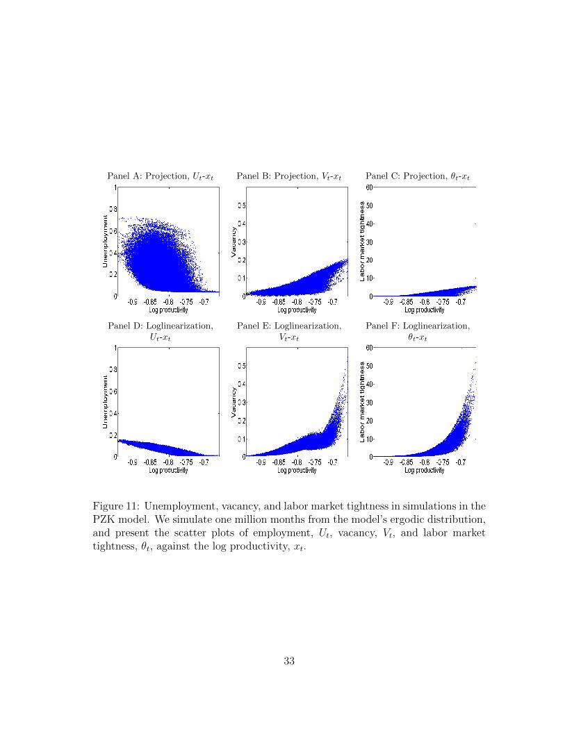
Panel A: Projection, Ut-xt Panel B: Projection, Vt-xt Panel C: Projection, θt-xt

Panel D: Loglinearization,Ut-xt

Panel E: Loglinearization,Vt-xt

Panel F: Loglinearization,θt-xt

Figure 11: Unemployment, vacancy, and labor market tightness in simulations in thePZK model. We simulate one million months from the model’s ergodic distribution,and present the scatter plots of employment, Ut, vacancy, Vt, and labor markettightness, θt, against the log productivity, xt.

33

spectively. We compute the responses to a one-standard-deviation shock to the logproductivity, both positive and negative, starting from a giving initial point. Theimpulse responses are averaged across 5,000 simulations, each with 60 months.

Figure 12 shows several important nonlinear patterns. First, the projection-based responses in unemployment are substantially stronger in the bad economythan in the good economy. In particular, in response to a negative impulse, theunemployment rate jumps up by 1.35% in the bad economy (Panel A), but only by0.035% in the good economy (Panel C). The maximum response in the median econ-omy is 0.215%, which is much closer to the good economy than to the bad economy.The large response in the bad economy is largely missed by loglinearization, whichimplies a maximum response of only 0.327%, less than 25% of the projection-basedresponse, 1.35%.

Second, the loglinearization-based responses in the market tightness, θt, are sub-stantially larger in the good economy than in the bad economy. In particular, inresponse to a positive impulse, θt jumps up by 2.38 in the good economy (PanelF), but only by 0.134 in the bad economy (Panel D). In contrast, the projectionalgorithm accurately captures the gradual nature of economic expansions. The max-imum response in the market tightness is 0.168 in the good economy, which is notfar from the response of 0.109 in the bad economy. Finally, wages are again inertialin the projection solution. Relative to projection, loglinearization vastly overstatesthe elasticity of wages in the good economy (Panel I).

Figure 13 shows that the projection-based responses in output, consumption,and investment are all stronger in the bad economy than in the good economy. Inparticular, in response to a positive impulse, output, consumption, and investmentrises by 2.23%, 1.72%, and 3.34% in the bad economy, in contrast to 0.68%, 0.42%,and 0.89%, respectively, in the good economy. Although close to the projection-based responses in the good economy, loglinearization understates the responsesin output, consumption, and investment in the bad economy to be 1.17%, 0.76%,and 1.76%, which are only 52.47%, 44.19%, and 52.69% of the projection-basedresponses, respectively.

3.6 Robustness

Our projection results are robust to choices in the grid parameters, as well as thebasis and degree of function approximation. Tables 5 and 6 report business cyclemoments and labor market moments, respectively, from each variation of the pro-jection algorithm. We vary the number of grid points for employment and capitalfrom 20 to 150, and the lower bound of the employment grid from 0.225 to 0.325.In each variation, we make sure that the lower bounds for both employment andcapital bind no more frequently than 0.02% in simulations. (In practice, the moregrid points that we use, the more frequently the lower bounds tend to bind in simu-

34

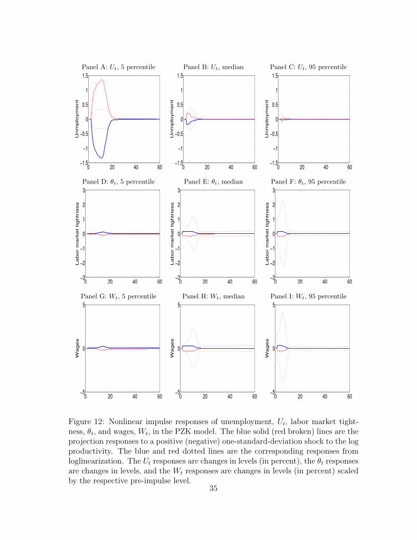
Panel A: Ut, 5 percentile Panel B: Ut, median Panel C: Ut, 95 percentile

0 20 40 60−1.5

−1

−0.5

0

0.5

1

1.5U

nm

plo

ym

ent

0 20 40 60−1.5

−1

−0.5

0

0.5

1

1.5

Unm

plo

ym

ent

0 20 40 60−1.5

−1

−0.5

0

0.5

1

1.5

Unm

plo

ym

ent

Panel D: θt, 5 percentile Panel E: θt, median Panel F: θt, 95 percentile

0 20 40 60−3

−2

−1

0

1

2

3

Labor m

arket tightn

ess

0 20 40 60−3

−2

−1

0

1

2

3

Labor m

arket tightn

ess

0 20 40 60−3

−2

−1

0

1

2

3

Labor m

arket tightn

ess

Panel G: Wt, 5 percentile Panel H: Wt, median Panel I: Wt, 95 percentile

0 20 40 60−5

0

5

Wages

0 20 40 60−5

0

5

Wages

0 20 40 60−5

0

5

Wages

Figure 12: Nonlinear impulse responses of unemployment, Ut, labor market tight-ness, θt, and wages, Wt, in the PZK model. The blue solid (red broken) lines are theprojection responses to a positive (negative) one-standard-deviation shock to the logproductivity. The blue and red dotted lines are the corresponding responses fromloglinearization. The Ut responses are changes in levels (in percent), the θt responsesare changes in levels, and the Wt responses are changes in levels (in percent) scaledby the respective pre-impulse level.

35

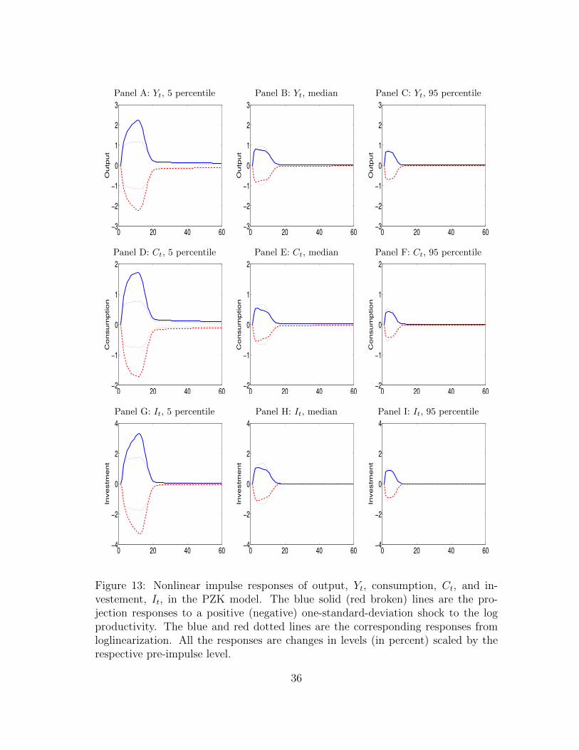
Panel A: Yt, 5 percentile Panel B: Yt, median Panel C: Yt, 95 percentile

0 20 40 60−3

−2

−1

0

1

2

3O

utp

ut

0 20 40 60−3

−2

−1

0

1

2

3

Outp

ut

0 20 40 60−3

−2

−1

0

1

2

3

Outp

ut

Panel D: Ct, 5 percentile Panel E: Ct, median Panel F: Ct, 95 percentile

0 20 40 60−2

−1

0

1

2

Consum

ption

0 20 40 60−2

−1

0

1

2

Consum

ption

0 20 40 60−2

−1

0

1

2

Consum

ption

Panel G: It, 5 percentile Panel H: It, median Panel I: It, 95 percentile

0 20 40 60−4

−2

0

2

4

Investm

ent

0 20 40 60−4

−2

0

2

4

Investm

ent

0 20 40 60−4

−2

0

2

4

Investm

ent

Figure 13: Nonlinear impulse responses of output, Yt, consumption, Ct, and in-vestement, It, in the PZK model. The blue solid (red broken) lines are the pro-jection responses to a positive (negative) one-standard-deviation shock to the logproductivity. The blue and red dotted lines are the corresponding responses fromloglinearization. All the responses are changes in levels (in percent) scaled by therespective pre-impulse level.

36

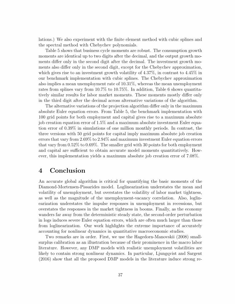
lations.) We also experiment with the finite element method with cubic splines andthe spectral method with Chebychev polynomials.

Table 5 shows that business cycle moments are robust. The consumption growthmoments are identical up to two digits after the decimal, and the output growth mo-ments differ only in the second digit after the decimal. The investment growth mo-ments also differ only in the second digit, except for the Chebychev approximation,which gives rise to an investment growth volatility of 4.37%, in contrast to 4.45% inour benchmark implementation with cubic splines. The Chebychev approximationalso implies a mean unemployment rate of 10.31%, whereas the mean unemploymentrates from splines vary from 10.7% to 10.75%. In addition, Table 6 shows quantita-tively similar results for labor market moments. These moments mostly differ onlyin the third digit after the decimal across alternative variations of the algorithm.

The alternative variations of the projection algorithm differ only in the maximumabsolute Euler equation errors. From Table 5, the benchmark implementation with100 grid points for both employment and capital gives rise to a maximum absolutejob creation equation error of 1.5% and a maximum absolute investment Euler equa-tion error of 0.39% in simulations of one million monthly periods. In contrast, thethree versions with 50 grid points for capital imply maximum absolute job creationerrors that vary from 2.69% to 2.94% and maximum investment Euler equation errorsthat vary from 0.52% to 0.69%. The smaller grid with 30 points for both employmentand capital are sufficient to obtain accurate model moments quantitatively. How-ever, this implementation yields a maximum absolute job creation error of 7.08%.

4 Conclusion

An accurate global algorithm is critical for quantifying the basic moments of theDiamond-Mortensen-Pissarides model. Loglinearization understates the mean andvolatility of unemployment, but overstates the volatility of labor market tightness,as well as the magnitude of the unemployment-vacancy correlation. Also, loglin-earization understates the impulse responses in unemployment in recessions, butoverstates the responses in the market tightness in booms. Finally, as the economywanders far away from the deterministic steady state, the second-order perturbationin logs induces severe Euler equation errors, which are often much larger than thosefrom loglinearization. Our work highlights the extreme importance of accuratelyaccounting for nonlinear dynamics in quantitative macroeconomic studies.

Two remarks are in order. First, we use the Hagedorn-Manovskii (2008) small-surplus calibration as an illustration because of their prominence in the macro laborliterature. However, any DMP models with realistic unemployment volatilities arelikely to contain strong nonlinear dynamics. In particular, Ljungqvist and Sargent(2016) show that all the proposed DMP models in the literature induce strong re-

37

sponses of unemployment to productivity shocks by diminishing the fundamentalsurplus, which is defined as the amount of output allocated to vacancy creation.The list of models includes Hagedorn and Manovskii, as well as the Hall (2005)sticky-wage model, the Hall-Milgrom (2008) alternating bargaining model, and thePissarides (2009) fixed matching costs model. As such, our insight on accuratelyaccounting for nonlinearities is general, not specific to Hagedorn and Manovskii.

Second, we focus on loglinearization and second-order perturbation because thesemethods are used extensively in the empirical macroeconomics literature (Chris-tiano, Eichenbaum, and Evans 2005; Smets and Wouters 2007). We emphasize thatour work is silent about the performance of high-order perturbations. Evaluating theperformance of state-of-the-art high-order perturbation methods against our accu-rate global algorithm in the context of the DMP model seems an important directionfor future research.

38

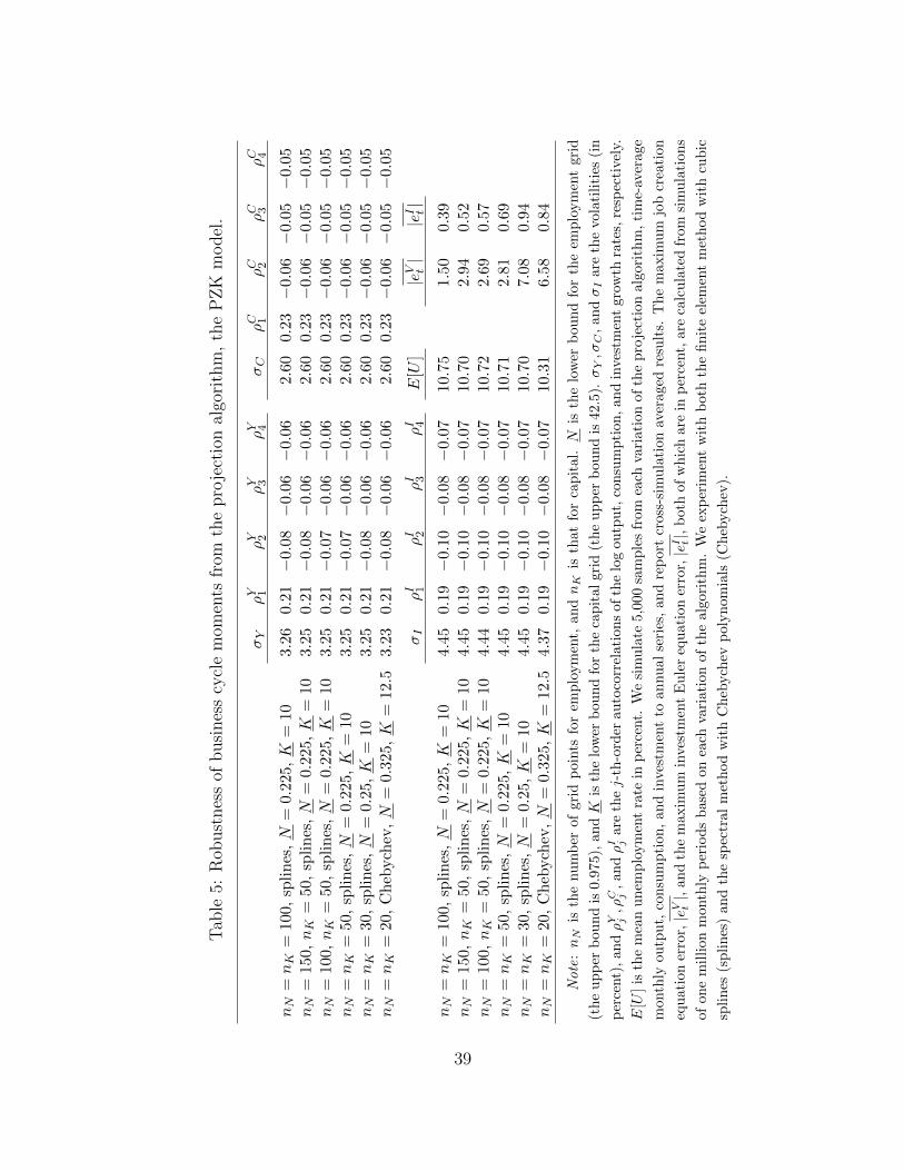
Tab

le5:

Rob

ust

nes

sof

busi

nes

scy

cle

mom

ents

from

the

pro

ject

ion

algo

rith

m,

the

PZ

Km

odel

.

σY

ρY 1

ρY 2

ρY 3

ρY 4

σC

ρC 1

ρC 2

ρC 3

ρC 4

nN

=nK

=10

0,sp

lin

es,N

=0.

225,K

=10

3.26

0.21−

0.08−

0.0

6−

0.0

62.

600.

23−

0.06−

0.0

5−

0.0

5nN

=15

0,nK

=50

,sp

lin

es,N

=0.

225,K

=10

3.25

0.21−

0.08−

0.0

6−

0.0

62.

600.

23−

0.06−

0.0

5−

0.0

5nN

=10

0,nK

=50

,sp

lin

es,N

=0.

225,K

=10

3.25

0.21−

0.07−

0.0

6−

0.0

62.

600.

23−

0.06−

0.0

5−

0.0

5nN

=nK

=50

,sp

lin

es,N

=0.

225,K

=10

3.25

0.21−

0.07−

0.0

6−

0.0

62.

600.

23−

0.06−

0.0

5−

0.0

5nN

=nK

=30

,sp

lin

es,N

=0.

25,K

=10

3.25

0.21−

0.08−

0.0

6−

0.0

62.

600.

23−

0.06−

0.0

5−

0.0

5nN

=nK

=20

,C

heb

ych

ev,N

=0.

325,K

=12.5

3.23

0.21−

0.08−

0.0

6−

0.0

62.

600.

23−

0.06−

0.0

5−

0.0

5

σI

ρI 1

ρI 2

ρI 3

ρI 4

E[U

]|eV t|

|eI t|

nN

=nK

=10

0,sp

lin

es,N

=0.

225,K

=10

4.45

0.19−

0.10−

0.0

8−

0.0

710

.75

1.5

00.3

9nN

=15

0,nK

=50

,sp

lin

es,N

=0.

225,K

=10

4.45

0.19−

0.10−

0.0

8−

0.0

710

.70

2.94

0.5

2nN

=10

0,nK

=50

,sp

lin

es,N

=0.

225,K

=10

4.44

0.19−

0.10−

0.0

8−

0.0

710

.72

2.69

0.5

7nN

=nK

=50

,sp

lin

es,N

=0.

225,K

=10

4.45

0.19−

0.10−

0.0

8−

0.0

710

.71

2.81

0.6

9nN

=nK

=30

,sp

lin

es,N

=0.

25,K

=10

4.45

0.19−

0.10−

0.0

8−

0.0

710

.70

7.08

0.9

4nN

=nK

=20

,C

heb

ych

ev,N

=0.

325,K

=12.5

4.37

0.19−

0.10−

0.0

8−

0.0

710

.31

6.58

0.8

4

Note

:nN

isth

enu

mb

erof

grid

poi

nts

for

emp

loym

ent,

an

dnK

isth

at

for

cap

ital.N

isth

elo

wer

bou

nd

for

the

emp

loym

ent

gri

d

(th

eu

pp

erb

oun

dis

0.97

5),

andK

isth

elo

wer

bou

nd

for

the

cap

ital

gri

d(t

he

up

per

bou

nd

is42.5

).σY,σ

C,

an

dσI

are

the

vola

tili

ties

(in

per

cent)

,an

dρY j,ρ

C j,an

dρI j

are

thej-

th-o

rder

au

toco

rrel

ati

on

sof

the

log

ou

tpu

t,co

nsu

mp

tion,an

din

vest

men

tgro

wth

rate

s,re

spec

tive

ly.

E[U

]is

the

mea

nu

nem

plo

ym

ent

rate

inp

erce

nt.

We

sim

ula

te5,0

00

sam

ple

sfr

om

each

vari

ati

on

of

the

pro

ject

ion

alg

ori

thm

,ti

me-

aver

age

mon

thly

outp

ut,

con

sum

pti

on,

and

inve

stm

ent

toan

nu

al

seri

es,

an

dre

port

cross

-sim

ula

tion

aver

aged

resu

lts.

Th

em

axim

um

job

crea

tion

equ

atio

ner

ror,|e

V t|,

and

the

max

imu

min

vest

men

tE

ule

req

uati

on

erro

r,|e

I t|,

both

of

wh

ich

are

inp

erce

nt,

are

calc

ula

ted

from

sim

ula

tion

s

ofon

em

illi

onm

onth

lyp

erio

ds

bas

edon

each

vari

ati

on

of

the

alg

ori

thm

.W

eex

per

imen

tw

ith

both

the

fin

ite

elem

ent

met

hod

wit

hcu

bic

spli

nes

(sp

lin

es)

and

the

spec

tral

met

hod

wit

hC

heb

ych

evp

oly

nom

ials

(Ch

ebych

ev).

39

Table 6: Robustness of labor market moments from the projection algorithm, thePZK model.

U V θ Y/N U V θ Y/N

nN = nK = 100, splines, nN = 150, nK = 50, splines,N = 0.225, K = 10 N = 0.225, K = 10

Standard deviation 0.158 0.158 0.254 0.010 0.158 0.158 0.254 0.010Autocorrelation 0.844 0.588 0.763 0.657 0.844 0.589 0.764 0.658

Correlation matrix −0.359 −0.473 −0.337 U −0.359 −0.473 −0.3380.899 0.983 V 0.899 0.983

0.930 θ 0.930

nN = 100, nK = 50, splines, nN = nK = 50, splines,N = 0.225, K = 10 N = 0.225, K = 10

Standard deviation 0.158 0.158 0.254 0.010 0.159 0.158 0.254 0.010Autocorrelation 0.844 0.589 0.764 0.658 0.844 0.589 0.764 0.658

Correlation matrix −0.359 −0.473 −0.338 U −0.358 −0.472 −0.3380.899 0.983 V 0.899 0.983

0.930 θ 0.930

nN = nK = 30, splines, nN = nK = 20, Chebychev,N = 0.25, K = 10 N = 0.325, K = 12.5

Standard deviation 0.159 0.158 0.254 0.010 0.160 0.157 0.254 0.010Autocorrelation 0.844 0.589 0.764 0.659 0.845 0.593 0.767 0.665

Correlation matrix −0.358 −0.472 −0.337 U −0.361 −0.474 −0.3410.898 0.982 V 0.899 0.981

0.929 θ 0.929

Note: nN is the number of grid points for employment, and nK is that for capital. N is the

lower bound for the employment grid (the upper bound is 0.975), and K is the lower bound for the

capital grid (the upper bound is 42.5). We simulate 5,000 artificial samples with 768 months in each

sample from each variation of the projection algorithm. We take the quarterly averages of monthly

unemployment U , vacancy, V , and labor productivity, Y/N , to convert to 256 quarters. θ = V/U

denotes labor market tightness. All the variables are in HP-filtered proportional deviations from

the mean with a smoothing parameter of 1,600. All the model moments are cross-simulation

averages. We experiment with both the finite element method with cubic splines (splines) and the

spectral method with Chebychev polynomials (Chebychev).

40

A Dynare programs

A.1 The HM model

// HM_loglinear.mod

var N, x, C;

predetermined_variables N;

varexo e;

parameters bet, rhox, stdx, eta, b, s, iota, kappa_K, kappa_W, xi;

bet = 0.99^(1/12);

rhox = 0.9895;

stdx = 0.0034;

eta = 0.052;

b = 0.955;

s = 0.0081;

iota = 0.407;

kappa_K = 0.474;

kappa_W = 0.11;

xi = 0.449;

model;

# kappa_t = kappa_K*exp(x) + kappa_W*(exp(x)^xi);

# V = (exp(x)*exp(N) - exp(C))/kappa_t;

# theta = V/(1 - exp(N));

# q = (1 + theta^iota)^(-1/iota);

# kappa_p = kappa_K*exp(x(+1)) + kappa_W*(exp(x(+1))^xi);

# V_p = ( exp(x(+1))*exp(N(+1)) - exp(C(+1)) )/kappa_p;

# theta_p = V_p/(1 - exp(N(+1)));

# q_p = (1 + theta_p^iota)^(-1/iota);

# W_p = eta*(exp(x(+1)) + kappa_p*theta_p) + (1 - eta)*b;

exp(N(+1)) = (1 - s)*exp(N) + q*V;

kappa_t/q = bet*( exp(x(+1)) - W_p + (1 - s)*kappa_p/q_p );

x = rhox*x(-1) + e;

end;

initval;

N = log(1 - 0.1);

x = 0;

e = 0;

end;

steady;

check;

shocks;

var e = stdx^2;

end;

41

stoch_simul (order = 1, nocorr, nomoments, IRF = 0);

For the second-order perturbation solution in logs, we change the last commandto:stoch_simul (order = 2, nocorr, nomoments, IRF = 0);

A.2 The PZK model

// PZK_loglinear.mod

var N, K, x, C, I, theta;

predetermined_variables N, K;

varexo e;

parameters beta, xbar, rhox, stdx, alpha, delta, nu, eta, s, iota, b, kappa;

beta = 0.99^(1/3);

xbar = -0.802;

rhox = 0.983047572491559;

stdx = 0.0065;

alpha = 1/3;

delta = 0.01;

nu = 2;

eta = 0.04;

s = 0.035;

iota = 1.25;

b = 0.95;

kappa = 0.45;

model;

# a1 = delta/(1 - nu);

# a2 = delta^(1/nu);

# Phi = (a1 + (a2/(1-1/nu))*((exp(I)/exp(K))^(1-1/nu)))*exp(K);

# q = (1 + exp(theta)^iota)^(-1/iota);

# qp = (1 + exp(theta(+1))^iota)^(-1/iota);

# Y = exp(x)*(exp(K)^alpha)*(exp(N)^(1 - alpha));

# V = (Y - exp(C) - exp(I))/kappa;

# M = beta*( exp(C)/exp(C(+1)) );

# Yp = exp(x(+1))*(exp(K(+1))^alpha)*(exp(N(+1))^(1 - alpha));

# Wp = eta*((1 - alpha)*Yp/exp(N(+1)) + kappa*exp(theta(+1))) + (1 - eta)*b;

exp(theta) = V/(1 - exp(N));

exp(N(+1)) = (1 - s)*exp(N) + q*V;

kappa/q = M*( (1 - alpha)*Yp/exp(N(+1)) - Wp + (1 - s)*kappa/qp );

exp(K(+1)) = (1 - delta)*exp(K) + Phi;

(1/a2)*((exp(I)/exp(K))^(1/nu)) = M*(alpha*Yp/exp(K(+1))

+ (1/a2)*((exp(I(+1))/exp(K(+1)))^(1/nu))*(1 - delta + a1)

+ (1/(nu-1))*exp(I(+1))/exp(K(+1)));

x = xbar*(1 - rhox) + rhox*x(-1) + e;

42

end;

initval;

N = log(1 - 0.048828933192708);

K = log(35.613860128463763);

x = xbar;

C = log(0.997225855318108);

I = log(0.356138601284638);

theta = log(2.234716290234390);

e = 0;

end;

steady;

check;

shocks;

var e = stdx^2;

end;

stoch_simul (order = 1, nocorr, nomoments, IRF = 0);

For the second-order perturbation solution in logs, we change the last commandto:stoch_simul (order = 2, nocorr, nomoments, IRF = 0);

43

References

Adjemian, S., H. Bastani, M. Juillard, F. Mihoubi, G. Perendia, M. Ratto, andS. Villemot (2011), “Dynare: Reference manual, version 4.” Dynare workingpaper 1, CEPREMAP.

Andolfatto, D. (1996), “Business cycles and labor-market search.” American Eco-nomic Review 86, 112–132.

Aruoba, S. B., J. Fernandez-Villaverde, and J. F. Rubio-Ramırez (2006), “Com-paring solution methods for dynamic equilibrium economies.” Journal of Eco-nomic Dynamic and Control 30, 2477–2508.

Blanchard, O. and J. Gali (2010), “Labor markets and monetary policy: A NewKeynesian model with unemployment.” American Economic Journal: Macroe-conomics 2, 1–30.

Caldara, D., J. Fernandez-Villaverde, J. F. Rubio-Ramırez, and W. Yao (2012),“Computing DSGE models with recursive preferences and stochastic volatil-ity.” Review of Economic Dynamics 15, 188-206.

Christiano, L. J., M. Eichenbaum, and C. L. Evans (2005), “Nominal rigiditiesand the dynamic effects of a shock to monetary policy.” Journal of PoliticalEconomy 113, 1-45.

Christiano, L. J. and J. D. M. Fisher (2000), “Algorithms for solving dynamic mod-els with occasionally binding constraints.” Journal of Economic Dynamics andControl 24, 1179–1232.

Cooley, T. F. and E. C. Prescott (1995), “Economic growth and business cycles.”in Thomas F. Cooley, ed. Frontiers of Business Cycle Research, PrincetonUniversity Press, Princeton, New Jersey.

Den Haan, W. J. (2010), “Comparison of solutions to the incomplete markets modelwith aggregate uncertainty.” Journal of Economic Dynamics and Control 34,4–27.

Den Haan, W. J. (2011), “Dynare.” lecture notes, London School of Economics.

Den Haan, W. J., G. Ramey, and J. Watson (2000), “Job destruction and propa-gation of shocks.” American Economic Review 90, 482–498.

Diamond, P. A. (1982), “Wage determination and efficiency in search equilibrium.”Review of Economic Studies 49, 217–227.

44

Fernandez-Villaverde, J. and O. Levintal (2016), “Solution methods for modelswith rare disasters.” NBER working paper.

Fernandez-Villaverde, J., J. F. Rubio-Ramırez, and F. Schorfheide (2016), “Solu-tion and estimation methods for DSGE models.” J. Taylor and H. Uhlig eds.,Handbook of Macroeconomics Volume 2, North-Holland, forthcoming.

Gertler, M. and A. Trigari (2009), “Unemployment fluctuations with staggeredNash wage bargaining.” Journal of Political Economy 117, 38–86.

Hagedorn, M. and I. Manovskii (2008), “The cyclical behavior of equilibrium un-employment and vacancies revisited.” American Economic Review 98, 1692–1706.

Hall, R. E. (2005), “Employment fluctuations with equilibrium wage stickiness.”American Economic Review 95, 50–65.

Hall, R. E. and P. R. Milgrom (2008), “The limited influence of unemployment onthe wage bargain.” American Economic Review 98, 1653–1674.

Hodrick, R. J. and E. C. Prescott (1997), “Postwar U.S. business cycles: An em-pirical investigation.” Journal of Money, Credit, and Banking 29, 1–16.

Judd, K. L. (1992), “Projection methods for solving aggregate growth models.”Journal of Economic Theory 58, 410–452.

Judd, K. L. (1998), Numerical Methods in Economics, The MIT Press, Cambridge,Massachusetts.

Judd, K. L., L. Maliar, S. Maliar, and R. Valero (2014), “Smolyak method for solv-ing dynamic economic models: Lagrange interpolation, anisotropic grid, andadaptive domain.” Journal of Economic Dynamics and Control 44, 92–123.

Kollmann, R., S. Maliar, B. A. Malin, and P. Pichler (2011), “Comparison of so-lutions to the multi-country real business cycle model.” Journal of EconomicDynamics and Control 35, 186–202.

Kopecky, K. A. and R. M. H. Suen (2010), “Finite state Markov-chain approxi-mations to highly persistent processes.” Review of Economic Dynamics 13,701–714.

Ljungqvist, L. and T. J. Sargent (2016), “The fundamental surplus.” workingpaper, New York University.

45

Maliar, S., L. Maliar, and K. L. Judd (2011), “Solving the multi-country real busi-ness cycle model using ergodic set methods.” Journal of Economic Dynamicsand Control 35, 207–228.

Malin, B. A., D. Krueger, and F. Kubler (2011), “Solving the multi-country realbusiness cycle model using a Smolyak-collocation method.” Journal of Eco-nomic Dynamics and Control 35, 229–239.

Merz, M. (1995), “Search in labor market and the real business cycle.” Journal ofMonetary Economics 95, 269–300.

Miranda, M. J. and P. L. Fackler (2002), Applied Computational Economics andFinance, The MIT Press, Cambridge, Massachusetts.

Monacelli, T., R. Perotti, and A. Trigari (2010), “Unemployment fiscal multipli-ers.” Journal of Monetary Economics 57, 531–553.

Mortensen, D. T. (1982), “The matching process as a noncooperative bargaininggame.” J. J. McCall, ed., The Economics of Information and Uncertainty,Chicago: University of Chicago Press, 233–254.

Mortensen, D. T. and E. Nagypal (2007), “More on unemployment and vacancyfluctuations.” Review of Economic Dynamics 10, 327–347.

Petrosky-Nadeau, N. and E. Wasmer (2013), “The cyclical volatility of labor mar-kets under frictional financial market.” American Economic Journal: Macroe-conomics 5, 193–221.

Petrosky-Nadeau, N., L. Zhang, and L. Kuehn (2015), “Endogenous disasters.”working paper, Federal Reserve Bank of San Francisco and The Ohio StateUniversity.

Petrosky-Nadeau, N. and L. Zhang (2016), “Unemployment crises.” working paper,Federal Reserve Bank of San Francisco and The Ohio State University.

Pichler, P. (2011), “Solving the multi-country real business cycle model using amonomial rule Galerkin method.” Journal of Economic Dynamics and Con-trol 35, 240–251.

Pissarides, C. A. (1985), “Short-run dynamics of unemployment, vacancies, andreal wages.” American Economic Review 75, 676–690.

Pissarides, C. A. (2009), “The unemployment volatility puzzle: Is wage stickinessthe answer?” Econometrica 77, 1339–1369.

46

Rouwenhorst, K. G. (1995), “Asset pricing implications of equilibrium business cy-cle models.” T. Cooley ed., Frontiers of Business Cycle Research, Princeton:Princeton University Press, 294–330.

Shimer, R. (2005), “The cyclical behavior of equilibrium unemployment and va-cancies.” American Economic Review 95, 25–49.

Smets, F. and R. Wouters (2007), “Shocks and frictions in US business cycles: ABayesian DSGE approach.” American Economic Review 97, 586–606.

Tauchen, G. (1986), “Finite state Markov-chain approximations to univariate andvector autoregressions.” Economics Letters 20, 177–181.

47