Embed Size (px)
Citation preview
Solving the Vehicle Routing Problem
with Genetic Algorithms
Áslaug Sóley Bjarnadóttir
April 2004
Informatics and Mathematical Modelling, IMM
Technical University of Denmark, DTU

Printed by IMM, DTU

3
Preface
This thesis is the final requirement for obtaining the degree Master of Science in Engineer-ing. The work was carried out at the section of Operations Research at Informatics andMathematical Modelling, Technical University of Denmark. The duration of the projectwas from the 10th of September 2003 to the 16th of April 2004. The supervisors wereJesper Larsen and Thomas Stidsen.
First of all, I would like to thank my supervisors for good ideas and suggestions throughoutthe project.
I would also like to thank Sigurlaug Kristjánsdóttir, Hildur Ólafsdóttir and Þórhallur IngiHalldórsson for correcting and giving comments on the report. Finally a want to thankmy fiance Ingólfur for great support and encouragement.
Odense, April 16th 2004
Áslaug Sóley Bjarnadóttir, s991139
4
Abstract
In this thesis, Genetic Algorithms are used to solve the Capacitated Vehicle RoutingProblem. The problem involves optimising a fleet of vehicles that are to serve a numberof customers from a central depot. Each vehicle has limited capacity and each customerhas a certain demand. Genetic Algorithms maintain a population of solutions by meansof a crossover and mutation operators.
A program is developed, based on a smaller program made by the author and a fellow stu-dent in the spring of 2003. Two operators are adopted from that program; Simple RandomCrossover and Simple Random Mutation. Additionally, three new crossover operators aredeveloped. They are named Biggest Overlap Crossover, Horizontal Line Crossover andUniform Crossover. Three Local Search Algorithms are also designed; Simple RandomAlgorithm, Non Repeating Algorithm and Steepest Improvement Algorithm. Then twosupporting operators Repairing Operator and Geographical Merge are made.
Steepest Improvement Algorithm is the most effective one of the Local Search Algorithms.The Simple Random Crossover with Steepest Improvement Algorithm performs best onsmall problems. The average difference from optimum or best known values is 4,16 ±1,22%. The Uniform Crossover with Steepest Improvement Crossover provided the best resultsfor large problems, where the average difference was 11.20±1,79%. The algorithms arecalled SRC-GA and UC-GA.
A comparison is made of SRC-GA, UC-GA, three Tabu Search heuristics and a new hybridgenetic algorithm, using a number of both small and large problems. SRC-GA and UC-GA are on average 10,52±5,48% from optimum or best known values and all the otherheuristics are within 1%. Thus, the algorithms are not effective enough. However, theyhave some good qualities, such as speed and simplicity. With that taken into account,they could make a good contribution to further work in the field.
5
Contents
1 Introduction 9
1.1 Outline of the Report . . . . . . . . . . . . . . . . . . . . . . . . . . . . . . 10
1.2 List of Abbreviations . . . . . . . . . . . . . . . . . . . . . . . . . . . . . . 11
2 Theory 13
2.1 The Vehicle Routing Problem . . . . . . . . . . . . . . . . . . . . . . . . . 13
2.1.1 The Problem . . . . . . . . . . . . . . . . . . . . . . . . . . . . . . 13
2.1.2 The Model . . . . . . . . . . . . . . . . . . . . . . . . . . . . . . . . 14
2.1.3 VRP in Real Life . . . . . . . . . . . . . . . . . . . . . . . . . . . . 15
2.1.4 Solution Methods and Literature Review . . . . . . . . . . . . . . . 16
2.2 Genetic Algorithms . . . . . . . . . . . . . . . . . . . . . . . . . . . . . . . 18
2.2.1 The Background . . . . . . . . . . . . . . . . . . . . . . . . . . . . 18
2.2.2 The Algorithm for VRP . . . . . . . . . . . . . . . . . . . . . . . . 19
2.2.3 The Fitness Value . . . . . . . . . . . . . . . . . . . . . . . . . . . . 21
2.2.4 Selection . . . . . . . . . . . . . . . . . . . . . . . . . . . . . . . . . 23
2.2.5 Crossover . . . . . . . . . . . . . . . . . . . . . . . . . . . . . . . . 26
2.2.6 Mutation . . . . . . . . . . . . . . . . . . . . . . . . . . . . . . . . 27
2.2.7 Inversion . . . . . . . . . . . . . . . . . . . . . . . . . . . . . . . . . 27
2.3 Summary . . . . . . . . . . . . . . . . . . . . . . . . . . . . . . . . . . . . 28
3 Local Search Algorithms 29
3.1 Simple Random Algorithm . . . . . . . . . . . . . . . . . . . . . . . . . . . 30
3.2 Non Repeating Algorithm . . . . . . . . . . . . . . . . . . . . . . . . . . . 31
3.3 Steepest Improvement Algorithm . . . . . . . . . . . . . . . . . . . . . . . 33
3.4 The Running Time . . . . . . . . . . . . . . . . . . . . . . . . . . . . . . . 34
6 CONTENTS
3.5 Comparison . . . . . . . . . . . . . . . . . . . . . . . . . . . . . . . . . . . 35
3.6 Summary . . . . . . . . . . . . . . . . . . . . . . . . . . . . . . . . . . . . 37
4 The Fitness Value and the Operators 39
4.1 The Fitness Value . . . . . . . . . . . . . . . . . . . . . . . . . . . . . . . . 40
4.2 The Crossover Operators . . . . . . . . . . . . . . . . . . . . . . . . . . . . 44
4.2.1 Simple Random Crossover . . . . . . . . . . . . . . . . . . . . . . . 45
4.2.2 Biggest Overlap Crossover . . . . . . . . . . . . . . . . . . . . . . . 46
4.2.3 Horizontal Line Crossover . . . . . . . . . . . . . . . . . . . . . . . 49
4.2.4 Uniform Crossover . . . . . . . . . . . . . . . . . . . . . . . . . . . 51
4.3 The Mutation Operator . . . . . . . . . . . . . . . . . . . . . . . . . . . . 55
4.3.1 Simple Random Mutation . . . . . . . . . . . . . . . . . . . . . . . 55
4.4 The Supporting Operators . . . . . . . . . . . . . . . . . . . . . . . . . . . 57
4.4.1 Repairing Operator . . . . . . . . . . . . . . . . . . . . . . . . . . . 57
4.4.2 Geographical Merge . . . . . . . . . . . . . . . . . . . . . . . . . . . 59
4.5 Summary . . . . . . . . . . . . . . . . . . . . . . . . . . . . . . . . . . . . 62
5 Implementation 63
6 Parameter Tuning 65
6.1 The Parameters and the Tuning Description . . . . . . . . . . . . . . . . . 65
6.2 The Results of Tuning . . . . . . . . . . . . . . . . . . . . . . . . . . . . . 69
6.3 Summary . . . . . . . . . . . . . . . . . . . . . . . . . . . . . . . . . . . . 70
7 Testing 71
7.1 The Benchmark Problems . . . . . . . . . . . . . . . . . . . . . . . . . . . 71
7.2 Test Description . . . . . . . . . . . . . . . . . . . . . . . . . . . . . . . . . 72
7.3 The Results . . . . . . . . . . . . . . . . . . . . . . . . . . . . . . . . . . . 73
7.3.1 Small Problems and Fast Algorithm . . . . . . . . . . . . . . . . . . 73
7.3.2 Small Problems and Slow Algorithm . . . . . . . . . . . . . . . . . 76
7.3.3 Comparison of Fast and Slow Algorithm for Small Problems. . . . . 79
7.3.4 Large Problems and Fast Algorithm . . . . . . . . . . . . . . . . . . 79
7.3.5 Large Problems and Slow Algorithm . . . . . . . . . . . . . . . . . 82
7.3.6 Comparison of Fast and Slow Algorithm for Large Problems. . . . . 84
CONTENTS 7
7.3.7 Comparison of the Algorithm and other Metaheuristics . . . . . . . 84
7.4 Summary . . . . . . . . . . . . . . . . . . . . . . . . . . . . . . . . . . . . 86
8 Discussion 87
8.1 Small Problems and Fast Algorithm . . . . . . . . . . . . . . . . . . . . . . 87
8.2 Small Problems and Slow Algorithm . . . . . . . . . . . . . . . . . . . . . 91
8.3 Large Problems and Fast Algorithm . . . . . . . . . . . . . . . . . . . . . . 91
8.4 Large Problems and Slow Algorithm . . . . . . . . . . . . . . . . . . . . . 93
8.5 The Results in general . . . . . . . . . . . . . . . . . . . . . . . . . . . . . 93
8.6 Summary . . . . . . . . . . . . . . . . . . . . . . . . . . . . . . . . . . . . 94
9 Conclusion 95
A Optimal Values for the Problem Instances in Chapter 3 99
B Results of Testing of Repairing Operator in Chapter 4 101
B.1 Simple Random Crossover . . . . . . . . . . . . . . . . . . . . . . . . . . . 101
B.2 Biggest Crossover Operator . . . . . . . . . . . . . . . . . . . . . . . . . . 102
C Results of Parameter Tuning 103
C.1 Combination 1, SRC, SRM, RO and SIA . . . . . . . . . . . . . . . . . . . 103
C.1.1 Small and Fast . . . . . . . . . . . . . . . . . . . . . . . . . . . . . 103
C.1.2 Small and Slow . . . . . . . . . . . . . . . . . . . . . . . . . . . . . 104
C.1.3 Large and Fast . . . . . . . . . . . . . . . . . . . . . . . . . . . . . 105
C.2 Combination 2, SRC, SRM and RO . . . . . . . . . . . . . . . . . . . . . . 106
C.2.1 Small and Fast . . . . . . . . . . . . . . . . . . . . . . . . . . . . . 106
C.2.2 Small and Slow . . . . . . . . . . . . . . . . . . . . . . . . . . . . . 108
C.2.3 Large and Fast . . . . . . . . . . . . . . . . . . . . . . . . . . . . . 109
C.3 Combination 3, BOC, SRM, RO and SIA . . . . . . . . . . . . . . . . . . . 109
C.3.1 Small and Fast . . . . . . . . . . . . . . . . . . . . . . . . . . . . . 109
C.3.2 Small and Slow . . . . . . . . . . . . . . . . . . . . . . . . . . . . . 111
C.3.3 Large and Fast . . . . . . . . . . . . . . . . . . . . . . . . . . . . . 112
C.4 Combination 4, BOC, SRM and RO . . . . . . . . . . . . . . . . . . . . . . 112
C.4.1 Small and Fast . . . . . . . . . . . . . . . . . . . . . . . . . . . . . 112
8 CONTENTS
C.4.2 Small and Slow . . . . . . . . . . . . . . . . . . . . . . . . . . . . . 114
C.4.3 Large and Fast . . . . . . . . . . . . . . . . . . . . . . . . . . . . . 115
C.5 Combination 5, HLC, SRM, GM and SIA . . . . . . . . . . . . . . . . . . . 115
C.5.1 Small and Fast . . . . . . . . . . . . . . . . . . . . . . . . . . . . . 115
C.5.2 Small and Slow . . . . . . . . . . . . . . . . . . . . . . . . . . . . . 117
C.5.3 Large and Fast . . . . . . . . . . . . . . . . . . . . . . . . . . . . . 118
C.6 Combination 6, HLC, SRM and GM . . . . . . . . . . . . . . . . . . . . . 118
C.6.1 Small and Fast . . . . . . . . . . . . . . . . . . . . . . . . . . . . . 118
C.6.2 Small and Slow . . . . . . . . . . . . . . . . . . . . . . . . . . . . . 120
C.6.3 Large and Fast . . . . . . . . . . . . . . . . . . . . . . . . . . . . . 121
C.7 Combination 7, UC, SRM, GM and SIA . . . . . . . . . . . . . . . . . . . 121
C.7.1 Small and Fast . . . . . . . . . . . . . . . . . . . . . . . . . . . . . 121
C.7.2 Small and Slow . . . . . . . . . . . . . . . . . . . . . . . . . . . . . 123
C.7.3 Large and Fast . . . . . . . . . . . . . . . . . . . . . . . . . . . . . 124
C.8 Combination 8, UFC, SRM and GM . . . . . . . . . . . . . . . . . . . . . 124
C.8.1 Small and Fast . . . . . . . . . . . . . . . . . . . . . . . . . . . . . 124
C.8.2 Small and Slow . . . . . . . . . . . . . . . . . . . . . . . . . . . . . 126
C.8.3 Large and Fast . . . . . . . . . . . . . . . . . . . . . . . . . . . . . 127
9
Chapter 1
Introduction
The agenda of this project is to design an efficient Genetic Algorithm to solve the VehicleRouting Problem. Many versions of the Vehicle Routing Problem have been described.The Capacitated Vehicle Routing Problem is discussed here and can in a simplified waybe described as follows: A fleet of vehicles is to serve a number of customers from a centraldepot. Each vehicle has limited capacity and each customer has a certain demand. A costis assigned to each route between every two customers and the objective is to minimizethe total cost of travelling to all the customers.
Real life Vehicle Routing Problems are usually so large that exact methods can not beused to solve them. For the past two decades, the emphasis has been on metaheuristics,which are methods used to find good solutions quickly. Genetic Algorithms belong to thegroup of metaheuristics. Relatively few experiments have been performed using GeneticAlgorithms to solve the Vehicle Routing Problem, which makes this approach interesting.Genetic Algorithms are inspired by the Theory of Natural Selection by Charles Darwin.A population of individuals or solutions is maintained by the means of crossover andmutation operators, where crossover simulates reproduction. The quality of each solutionis indicated by a fitness value. This value is used to select a solution from the populationto reproduce and when solutions are excluded from the population. The average qualityof the population gradually improves as new and better solutions are generated and worsesolutions are removed.
The project is based on a smaller project developed by the author and Hildur Ólafsdóttirin the course Large-Scale Optimization at DTU in the spring of 2003. In that projecta small program was developed, which simulates Genetic Algorithms using very simplecrossover and mutation operators. This program forms the basis of the current project.
In this project new operators are designed in order to focus on the geography of theproblem, which is relevant to the Capacitated Vehicle Routing Problem. The operatorsare developed using a trial and error method and experiments are made in order tofind out which characteristics play a significant role in a good algorithm. A few LocalSearch Algorithms are also designed and implemented in order to increase the efficiency.Additionally, an attention is paid to the fitness value and how it influences the performanceof the algorithm. The aim of the project is described by the following hypothesis:
10 Chapter 1. Introduction
It is possible to develop operators for Genetic Algorithms efficient enough to solve large
Vehicle Routing Problems.
Problem instances counting more than 100 customers are considered large. What isefficient enough? Most heuristics are measured against the criteria accuracy and speed.Cordeau et al. [4] remark that simplicity and flexibility are also important characteristicsof heuristics. The emphasis here is mostly on accuracy. The operators are consideredefficient enough if they are able to compete with the best results proposed in the literature.However, an attempt is also made to measure the quality of the operators by the meansof the other criteria.
1.1 Outline of the Report
In chapter 2 the theory of the Vehicle Routing Problem and the Genetic Algorithms isdiscussed. Firstly, the Vehicle Routing Problem is described, the model presented anda review of the literature given among other things. Secondly, the basic concepts of theGenetic Algorithms are explained and different approaches are discussed, e.g. when itcomes to choosing a fitness value or a selection method. Then the different types ofoperators are introduced.
The Local Search Algorithms are presented in chapter 3. Three different algorithms areexplained both in words and by a pseudocode. They are compared and the best onechosen for further use.
Chapter 4 describes the development process of the fitness value and the operators. Fourcrossover operators are explained and in addition; a mutation operator and two supportingoperators. All operators are explained both in words and by the means of a pseudocode.
Implementation issues are discussed in chapter 5. This includes information about thecomputer used for testing, programming language and some relevant methods.
The parameter tuning is described in chapter 6. At first the possible parameters are listedand the procedure of tuning is explained. Then the resulting parameters are illustrated.
Chapter 7 involves the final testing. It starts with a listing of benchmark problems followedby a test description. Then test results are presented. Firstly, different combinations ofoperators are used to solve a few problems in order to choose the best combination.Secondly, this best combination is applied to a large number of problems. Finally, theseresults are compared to results presented in the literature.
The results are discussed in chapter 8 and in chapter 9 the conclusion in presented.
1.2 List of Abbreviations 11
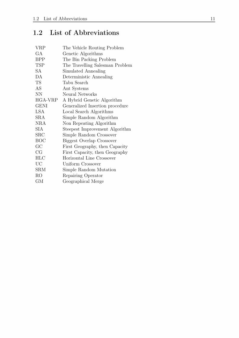
1.2 List of Abbreviations
VRP The Vehicle Routing ProblemGA Genetic AlgorithmsBPP The Bin Packing ProblemTSP The Travelling Salesman ProblemSA Simulated AnnealingDA Deterministic AnnealingTS Tabu SearchAS Ant SystemsNN Neural NetworksHGA-VRP A Hybrid Genetic AlgorithmGENI Generalized Insertion procedureLSA Local Search AlgorithmsSRA Simple Random AlgorithmNRA Non Repeating AlgorithmSIA Steepest Improvement AlgorithmSRC Simple Random CrossoverBOC Biggest Overlap CrossoverGC First Geography, then CapacityCG First Capacity, then GeographyHLC Horizontal Line CrossoverUC Uniform CrossoverSRM Simple Random MutationRO Repairing OperatorGM Geographical Merge

12 Chapter 1. Introduction
13
Chapter 2
Theory
The aim of this chapter is to present the Vehicle Routing Problem (VRP) and GeneticAlgorithms (GA) in general. Firstly, VRP is introduced and its model is put forward.Then the nature of the problem is discussed and a review of literature is given. Secondly,GA are introduced and fitness value, selection methods and operators are addressed.
2.1 The Vehicle Routing Problem
2.1.1 The Problem
The Vehicle Routing Problem was first introduced by Dantzig and Ramser in 1959 [12]and it has been widely studied since. It is a complex combinatorial optimisation problem.Fisher [7] describes the problem in a word as to find the efficient use of a fleet of vehiclesthat must make a number of stops to pick up and/or deliver passengers or products. Theterm customer will be used to denote the stops to pick up and/or deliver. Every customerhas to be assigned to exactly one vehicle in a specific order. That is done with respect tothe capacity and in order to minimise the total cost.
The problem can be considered as a combination of the two well-known optimisationproblems; the Bin Packing Problem (BPP) and the Travelling Salesman Problem (TSP).The BPP is described in the following way: Given a finite set of numbers (the item sizes)and a constant K, specifying the capacity of the bin, what is the minimum number of binsneeded?[6] Naturally, all items have to be inside exactly one bin and the total capacityof items in each bin has to be within the capacity limits of the bin. This is known asthe best packing version of BPP. The TSP is about a travelling salesman who wants tovisit a number of cities. He has to visit each city exactly once, starting and ending in hishome town. The problem is to find the shortest tour through all cities. Relating this tothe VRP, customers can be assigned to vehicles by solving BPP and the order in whichthey are visited can be found by solving TSP.
Figure 2.1 shows a solution to a VRP as a graph.
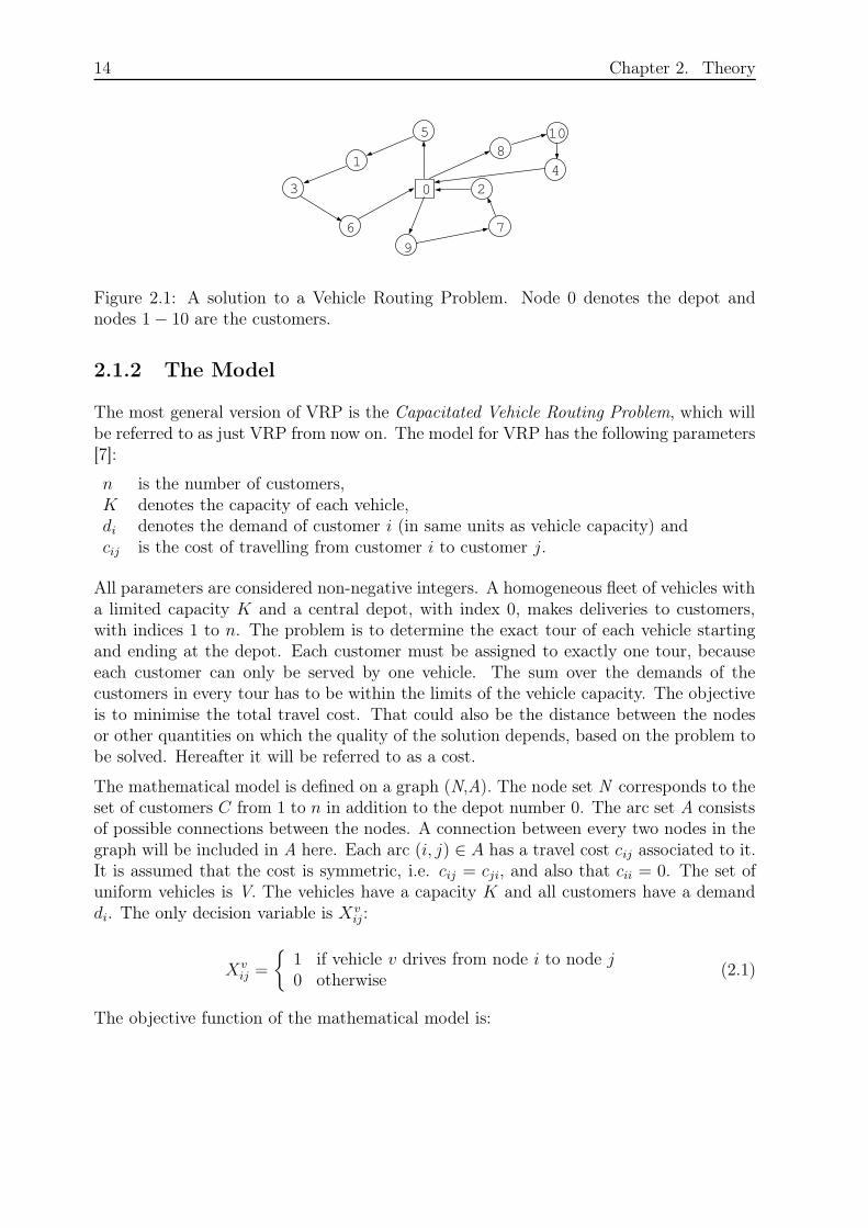
14 Chapter 2. Theory
0
1
6
3
5
7
9
810
42
Figure 2.1: A solution to a Vehicle Routing Problem. Node 0 denotes the depot andnodes 1− 10 are the customers.
2.1.2 The Model
The most general version of VRP is the Capacitated Vehicle Routing Problem, which willbe referred to as just VRP from now on. The model for VRP has the following parameters[7]:
n is the number of customers,K denotes the capacity of each vehicle,di denotes the demand of customer i (in same units as vehicle capacity) andcij is the cost of travelling from customer i to customer j.
All parameters are considered non-negative integers. A homogeneous fleet of vehicles witha limited capacity K and a central depot, with index 0, makes deliveries to customers,with indices 1 to n. The problem is to determine the exact tour of each vehicle startingand ending at the depot. Each customer must be assigned to exactly one tour, becauseeach customer can only be served by one vehicle. The sum over the demands of thecustomers in every tour has to be within the limits of the vehicle capacity. The objectiveis to minimise the total travel cost. That could also be the distance between the nodesor other quantities on which the quality of the solution depends, based on the problem tobe solved. Hereafter it will be referred to as a cost.
The mathematical model is defined on a graph (N,A). The node set N corresponds to theset of customers C from 1 to n in addition to the depot number 0. The arc set A consistsof possible connections between the nodes. A connection between every two nodes in thegraph will be included in A here. Each arc (i, j) ∈ A has a travel cost cij associated to it.It is assumed that the cost is symmetric, i.e. cij = cji, and also that cii = 0. The set ofuniform vehicles is V. The vehicles have a capacity K and all customers have a demanddi. The only decision variable is Xv
ij:
Xvij =
{
1 if vehicle v drives from node i to node j0 otherwise
(2.1)
The objective function of the mathematical model is:
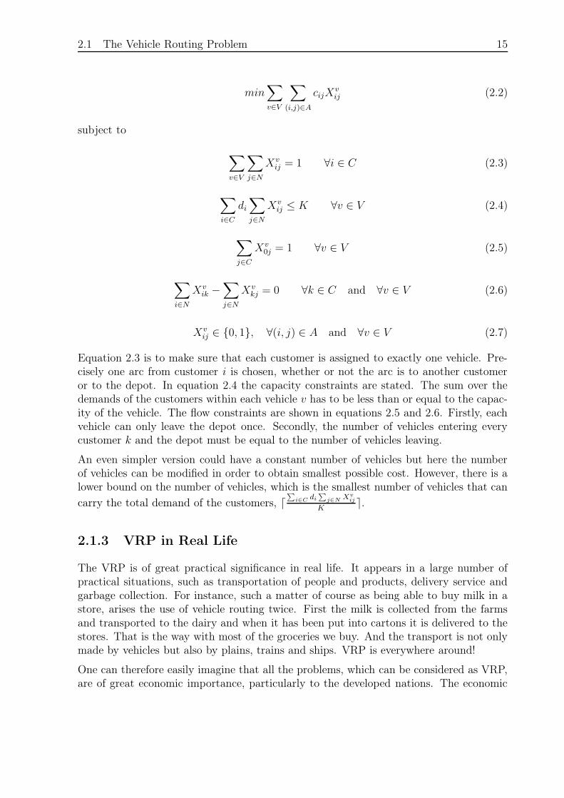
2.1 The Vehicle Routing Problem 15
min∑
v∈V
∑
(i,j)∈A
cijXvij (2.2)
subject to
∑
v∈V
∑
j∈N
Xvij = 1 ∀i ∈ C (2.3)
∑
i∈C
di
∑
j∈N
Xvij ≤ K ∀v ∈ V (2.4)
∑
j∈C
Xv0j = 1 ∀v ∈ V (2.5)
∑
i∈N
Xvik −
∑
j∈N
Xvkj = 0 ∀k ∈ C and ∀v ∈ V (2.6)
Xvij ∈ {0, 1}, ∀(i, j) ∈ A and ∀v ∈ V (2.7)
Equation 2.3 is to make sure that each customer is assigned to exactly one vehicle. Pre-cisely one arc from customer i is chosen, whether or not the arc is to another customeror to the depot. In equation 2.4 the capacity constraints are stated. The sum over thedemands of the customers within each vehicle v has to be less than or equal to the capac-ity of the vehicle. The flow constraints are shown in equations 2.5 and 2.6. Firstly, eachvehicle can only leave the depot once. Secondly, the number of vehicles entering everycustomer k and the depot must be equal to the number of vehicles leaving.
An even simpler version could have a constant number of vehicles but here the numberof vehicles can be modified in order to obtain smallest possible cost. However, there is alower bound on the number of vehicles, which is the smallest number of vehicles that can
carry the total demand of the customers, d∑
i∈C di
∑
j∈N Xvij
Ke.
2.1.3 VRP in Real Life
The VRP is of great practical significance in real life. It appears in a large number ofpractical situations, such as transportation of people and products, delivery service andgarbage collection. For instance, such a matter of course as being able to buy milk in astore, arises the use of vehicle routing twice. First the milk is collected from the farmsand transported to the dairy and when it has been put into cartons it is delivered to thestores. That is the way with most of the groceries we buy. And the transport is not onlymade by vehicles but also by plains, trains and ships. VRP is everywhere around!
One can therefore easily imagine that all the problems, which can be considered as VRP,are of great economic importance, particularly to the developed nations. The economic
16 Chapter 2. Theory
importance has been a great motivation for both companies and researches to try to findbetter methods to solve VRP and improve the efficiency of transportation.
2.1.4 Solution Methods and Literature Review
The model above describes a very simple version of VRP. In real life, VRP can havemany more complications, such as asymmetric travel costs, multiple depots, heterogeneousvehicles and time windows, associated with each customer. These possible complicationsmake the problem more difficult to solve. They are not considered in this project becausethe emphasis is rather on Genetic Algorithms.
In section 2.1.1 above, it is explained how VRP can be considered a merge of BPP andTSP. Both BPP and TSP are so-called NP-hard problems [6] and [21], thus VRP is alsoNP-hard. NP-hard problems are difficult to solve and in fact it means that to date nooptimal algorithm has been found, which is able to solve the problem in polynomial time[6]. Finding an optimal solution to a NP-hard problem is usually very time consumingor even impossible. Because of this nature of the problem, it is not realistic to use exactmethods to solve large instances of the problem. For small instances of only few customers,the branch and bound method has proved to be the best [15]. Most approaches for largeinstances are based on heuristics. Heuristics are approximation algorithms that aim atfinding good feasible solutions quickly. They can be roughly divided into two main classes;classical heuristics mostly from between 1960 and 1990 and metaheuristics from 1990 [12].
The classical heuristics can be divided into three groups; Construction methods, two-phase methods and improvement methods [13]. Construction methods gradually build afeasible solution by selecting arcs based on minimising cost, like the Nearest Neighbour[11] method does. The two-phase method divides the problem into two parts; clusteringof customers into feasible routes disregarding their order and route construction. Anexample of a two-phase method is the Sweep Algorithm [12], which will be discussedfurther in section 4.2.3. The Local Search Algorithms [1], explained in chapter 3, belongto the improvement heuristics. They start with a feasible solution and try to improve itby exchanging arcs or nodes within or between the routes. The advantage of the classicalheuristics is that they have a polynomial running time, thus using them one is better ableto provide good solutions within a reasonable amount of time [4]. On the other hand, theyonly do a limited search in the solution space and do therefore run the risk of resultingin a local optimum.
Metaheuristics are more effective and specialised than the classical heuristics [5]. Theycombine more exclusive neighbourhood search, memory structures and recombination ofsolutions and tend to provide better results, e.g. by allowing deterioration and even in-feasible solutions [10]. However, their running time is unknown and they are usually moretime consuming than the classical heuristics. Furthermore, they involve many parametersthat need to be tuned for each problem before they can be applied.
For the last ten years metaheuristics have been researched considerably, producing someeffective solution methods for VRP [4]. At least six metaheuristics have been applied to
2.1 The Vehicle Routing Problem 17
VRP; Simulated Annealing (SA), Deterministic Annealing (DA), Tabu Search (TS), AntSystems (AS), Neural Networks (NN) and Genetic Algorithms (GA) [10]. The algorithmsSA, DA and TS move from one solution to another one in the neighbourhood until a stop-ping criterion is satisfied. The fourth method, AS, is a constructive mechanism creatingseveral solutions in each iteration based on information from previous generations. NN isa learning method, where a set of weights is gradually adjusted until a satisfactory solu-tion is reached. Finally, GA maintain a population of good solutions that are recombinedto produce new solutions.
Compared to best-known methods, SA, DA and AS have not shown competitive resultsand NN are clearly outperformed [10]. TS has got a lot of attention by researches and sofar it has proved to be the most effective approach for solving VRP [4]. Many differentTS heuristics have been proposed with unequal success. The general idea of TS and afew variants thereof are discussed below. GA have been researched considerably, butmostly in order to solve TSP and VRP with time windows [2], where each customerhas a time window, which the vehicle has to arrive in. Although they have succeededin solving VRP with time windows, they have not been able to show as good resultsfor the capacitated VRP. In 2003 Berger and Barkaoui presented a new Hybrid GeneticAlgorithm (HGA-VRP) to solve the capacitated VRP [2]. It uses two populations ofsolutions that periodically exchange some number of individuals. The algorithm hasshown to be competitive in comparison to the best TS heuristics [2]. In the next twosubsections three TS approaches are discussed followed by a further discussion of HGA-VRP.
Tabu Search
As written above, to date Tabu Search has been the best metaheuristic for VRP [4]. Theheuristic starts with an initial solution x1 and in step t it moves from solution xt to thebest solution xt+1 in its neighbourhood N(xt), until a stopping criterion is satisfied. Iff(xt) denotes the cost of solution xt, f(xt+1) does not necessarily have to be less thanf(xt). Therefore, a cycling must be prevented, which is done by declaring some recentlyexamined solutions tabu or forbidden and storing them in a tabulist. Usually, the TSmethods preserve an attribute of a solution in the tabulist instead of the solution itselfto save time and memory. Different TS heuristics have been proposed not all with equalsuccess. For the last decade, some successful TS heuristics have been proposed [12].
The Taburoute of Gendreau et al. [9] is an involved heuristic with some innovative features.It defines the neighbourhood of xt as a set of solutions that can be reached from xt byremoving a customer k from its route r and inserting it into another route s containingone of its nearest neighbours. The method uses Generalised Insertion (GENI) procedurealso developed by Gendreau et al. [8]. Reinsertion of k into r is forbidden for the next θiterations, where θ is a random integer in the interval (5,10) [12]. A diversification strategyis used to penalise frequently moved nodes. The Taburoute produces both feasible andinfeasible solutions.
The Taillard’s Algorithm is one of the most accurate TS heuristics [4]. Like Taburoute
18 Chapter 2. Theory
it uses random tabu duration and diversification. However, the neighbourhood is definedby the means of λ-interchange generation mechanism and standard insertion methods areused instead of GENI. The innovative feature of the algorithm is the decomposition ofthe main problem into subproblems.
The Adaptive Memory procedure of Rochat and Taillard is the last TS heuristic that willbe discussed here. It is probably one of the most interesting novelties that have emergedwithin TS heuristics in recent years [12]. An adaptive memory is a pool of solutions, whichis dynamically updated during the search process by combining some of the solutions inthe pool in order to produce some new good solutions. Therefore, it can be considered ageneralisation of the genetic search.
A Hybrid Genetic Algorithm
The Hybrid Genetic Algorithm proposed by Berger and Barkaoui is able to solve VRP inalmost as effective way as TS [2]. Genetic Algorithms are explained in general in the nextsection. The algorithm maintains two populations of solutions that exchange a numberof solutions at the end of each iteration. New solutions are generated by rather complexoperators that have successfully been used to solve the VRP with time windows. Whena new best solution has been found the customers are reordered for further improvement.In order to have a constant number of solutions in the populations the worst individualsare removed. For further information about the Hybrid Genetic Algorithm the reader isreferred to [2].
2.2 Genetic Algorithms
2.2.1 The Background
The Theory of Natural Selection was proposed by the British naturalist Charles Dar-win (1809-1882) in 1859 [3]. The theory states that individuals with certain favourablecharacteristics are more likely to survive and reproduce and consequently pass their char-acteristics on to their offsprings. Individuals with less favourable characteristics willgradually disappear from the population. In nature, the genetic inheritance is stored inchromosomes, made of genes. The characteristics of every organism is controlled by thegenes, which are passed on to the offsprings when the organisms mate. Once in a while amutation causes a change in the chromosomes. Due to natural selection, the populationwill gradually improve on the average as the number of individuals having the favourablecharacteristics increases.
The Genetic Algorithms (GA) were invented by John Holland and his colleagues in theearly 1970s [16], inspired by Darwin’s theory. The idea behind GA is to model thenatural evolution by using genetic inheritance together with Darwin’s theory. In GA,the population consists of a set of solutions or individuals instead of chromosomes. Acrossover operator plays the role of reproduction and a mutation operator is assigned
2.2 Genetic Algorithms 19
to make random changes in the solutions. A selection procedure, simulating the naturalselection, selects a certain number of parent solutions, which the crossover uses to generatenew solutions, also called offsprings. At the end of each iteration the offsprings togetherwith the solutions from the previous generation form a new generation, after undergoing aselection process to keep a constant population size. The solutions are evaluated in termsof their fitness values identical to the fitness of individuals.
The GA are adaptive learning heuristic and they are generally referred to in plural, becauseseveral versions exist that are adjustments to different problems. They are also robustand effective algorithms that are computationally simple and easy to implement. Thecharacteristics of GA that distinguishes them from the other heuristics, are the following[16]:
• GA work with coding of the solutions instead of the solution themselves. Therefore,a good, efficient representation of the solutions in the form of a chromosome isrequired.• They search from a set of solutions, different from other metaheuristics like Sim-
ulated annealing and Tabu search that start with a single solution and move toanother solution by some transition. Therefore they do a multi directional searchin the solution space, reducing the probability of finishing in a local optimum.• They only require objective function values, not e.g. continuous searching space
or existence of derivatives. Real life examples generally have discontinuous searchspaces.• GA are nondeterministic, i.e. they are stochastic in decisions, which makes them
more robust.• They are blind because they do not know when they have found an optimal solution.
2.2.2 The Algorithm for VRP
As written above, GA easily adapts to different problems so there are many differentversions depending on the problem to solve. There are, among other things, several waysto maintain a population and many different operators can be applied. But all GA musthave the following basic items that need to be carefully considered for the algorithm towork as effective as possible [14]:
• A good genetic representation of a solution in a form of a chromosome.• An initial population constructor.• An evaluation function to determine the fitness value for each solution.• Genetic operators, simulating reproduction and mutation.• Values for parameters; population size, probability of using operators, etc.
A good representation or coding of VRP solution must identify the number of vehicles,which customers are assigned to each vehicle and in which order they are visited. Some-times solutions are represented as binary strings, but that kind of representation does notsuit VRP well. It is easy to specify the number of vehicles and which customers are insideeach vehicle but it becomes too complicated when the order of the customers needs to be
20 Chapter 2. Theory
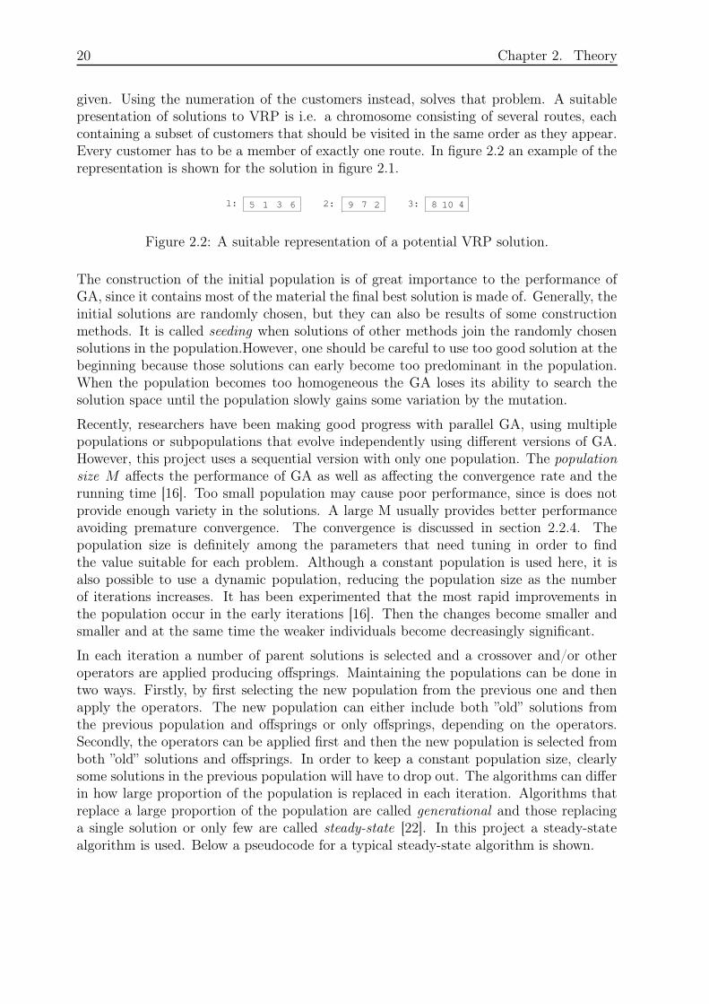
given. Using the numeration of the customers instead, solves that problem. A suitablepresentation of solutions to VRP is i.e. a chromosome consisting of several routes, eachcontaining a subset of customers that should be visited in the same order as they appear.Every customer has to be a member of exactly one route. In figure 2.2 an example of therepresentation is shown for the solution in figure 2.1.
5 8279631 10 41: 2: 3:
Figure 2.2: A suitable representation of a potential VRP solution.
The construction of the initial population is of great importance to the performance ofGA, since it contains most of the material the final best solution is made of. Generally, theinitial solutions are randomly chosen, but they can also be results of some constructionmethods. It is called seeding when solutions of other methods join the randomly chosensolutions in the population.However, one should be careful to use too good solution at thebeginning because those solutions can early become too predominant in the population.When the population becomes too homogeneous the GA loses its ability to search thesolution space until the population slowly gains some variation by the mutation.
Recently, researchers have been making good progress with parallel GA, using multiplepopulations or subpopulations that evolve independently using different versions of GA.However, this project uses a sequential version with only one population. The populationsize M affects the performance of GA as well as affecting the convergence rate and therunning time [16]. Too small population may cause poor performance, since is does notprovide enough variety in the solutions. A large M usually provides better performanceavoiding premature convergence. The convergence is discussed in section 2.2.4. Thepopulation size is definitely among the parameters that need tuning in order to findthe value suitable for each problem. Although a constant population is used here, it isalso possible to use a dynamic population, reducing the population size as the numberof iterations increases. It has been experimented that the most rapid improvements inthe population occur in the early iterations [16]. Then the changes become smaller andsmaller and at the same time the weaker individuals become decreasingly significant.
In each iteration a number of parent solutions is selected and a crossover and/or otheroperators are applied producing offsprings. Maintaining the populations can be done intwo ways. Firstly, by first selecting the new population from the previous one and thenapply the operators. The new population can either include both ”old” solutions fromthe previous population and offsprings or only offsprings, depending on the operators.Secondly, the operators can be applied first and then the new population is selected fromboth ”old” solutions and offsprings. In order to keep a constant population size, clearlysome solutions in the previous population will have to drop out. The algorithms can differin how large proportion of the population is replaced in each iteration. Algorithms thatreplace a large proportion of the population are called generational and those replacinga single solution or only few are called steady-state [22]. In this project a steady-statealgorithm is used. Below a pseudocode for a typical steady-state algorithm is shown.
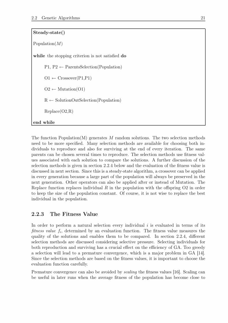
2.2 Genetic Algorithms 21
Steady-state()
Population(M)
while the stopping criterion is not satisfied do
P1, P2 ← ParentsSelection(Population)
O1 ← Crossover(P1,P1)
O2 ← Mutation(O1)
R ← SolutionOutSelection(Population)
Replace(O2,R)
end while
The function Population(M) generates M random solutions. The two selection methodsneed to be more specified. Many selection methods are available for choosing both in-dividuals to reproduce and also for surviving at the end of every iteration. The sameparents can be chosen several times to reproduce. The selection methods use fitness val-ues associated with each solution to compare the solutions. A further discussion of theselection methods is given in section 2.2.4 below and the evaluation of the fitness value isdiscussed in next section. Since this is a steady-state algorithm, a crossover can be appliedin every generation because a large part of the population will always be preserved in thenext generation. Other operators can also be applied after or instead of Mutation. TheReplace function replaces individual R in the population with the offspring O2 in orderto keep the size of the population constant. Of course, it is not wise to replace the bestindividual in the population.
2.2.3 The Fitness Value
In order to perform a natural selection every individual i is evaluated in terms of itsfitness value fi, determined by an evaluation function. The fitness value measures thequality of the solutions and enables them to be compared. In section 2.2.4, differentselection methods are discussed considering selective pressure. Selecting individuals forboth reproduction and surviving has a crucial effect on the efficiency of GA. Too greedya selection will lead to a premature convergence, which is a major problem in GA [14].Since the selection methods are based on the fitness values, it is important to choose theevaluation function carefully.
Premature convergence can also be avoided by scaling the fitness values [16]. Scaling canbe useful in later runs when the average fitness of the population has become close to
22 Chapter 2. Theory
the fitness of the optimal solution and thus the average and the best individuals of thepopulation are almost equally likely to be chosen. Naturally, the evaluation function andscaling of fitness values work together. Several scaling methods have been introduced,e.g. linear scaling, with and without sigma truncation and power law scaling [14].
The linear scaling method scales the fitness value fi as follows:
f ′
i = a× fi + b (2.8)
where a and b are chosen so that the average initial fitness and the scaled fitness are equal.The linear scaling method is quite good but it runs into problems in later iterations whensome individuals have very low fitness values close to each other, resulting in negativefitness values [14]. Also, the parameters a and b depend only on the population but noton the problem.
The sigma truncation method deals with this problem by mapping the fitness value intoa modified fitness value f ′′
i with the following formula:
f ′′
i = fi − (f −Kmult × σ) (2.9)
Kmult is a multiplying constant, usually between 1 and 5 [14]. The method includes theaverage fitness f of the population and the standard deviation σ, which makes the scalingproblem dependent. Possible negative values are set equal to zero. The linear scaling isnow applied with f ′′
i instead of f ′
i .
Finally, there is the power law scaling method, which scales the fitness value by raising itto the power of k, depending on the problem.
f ′
i = f ki (2.10)
Often, it is straightforward to find an evaluation function to determine the fitness value.For many optimisation problems the evaluation function for a feasible solution is given,i.e. for both TSP and VRP, the most obvious fitness value is simply the total cost ordistance travelled. However, this is not always the case, especially when dealing withmulti objective problems and/or infeasible solutions.
There are two ways to handle infeasible solutions; either rejecting them or penalisingthem. Rejecting infeasible solutions simplifies the algorithm and might work out well ifthe feasible search space is convex [14]. On the other hand, it can have some significantlimitations, because allowing the algorithm to cross the infeasible region can often enableit to reach the optimal solution.
Dealing with infeasible solutions can be done in two ways. Firstly, by extending thesearching space over the infeasible region as well. The evaluation function for an infeasiblesolution evalu(x) is the sum of the fitness value of the feasible solution evalf(x) and eitherthe penalty or the cost of repairing an infeasible individual Q(x), i.e.
evalu(x) = evalf (x)±Q(x) (2.11)
2.2 Genetic Algorithms 23
Designing the penalty function is far from trivial. It should be kept as low as possiblewithout allowing the algorithm to converge towards infeasible solutions. It can be difficultto find the balance in between. Secondly, another evaluation function can be designed,independent of the evaluation function for the feasible solution evalf .
Both methods require a relationship between the evaluation functions established, whichis among the most difficult problems when using GA. The relationship can either beestablished using an equation or by constructing a global evaluation function:
eval(x) =
{
q1 · evalf (x) if x ∈ Fq2 · evalu(x) if x ∈ U
(2.12)
The weights q1 and q2 scale the relative importance of evalf and evalu and F and Udenote the feasible region and the infeasible region respectively.
The problem with both methods is that they allow an infeasible solution to have a betterfitness value than a feasible one. Thus, the algorithm can in the end converge towardsan infeasible final solution. Comparing solutions can also be risky. Sometimes it is notquite clear whether a feasible individual is better than an infeasible one, if an infeasibleindividual is extremely close to the optimal solution. Furthermore, it can be difficult tocompare two infeasible solutions. Consider two solutions to the 0-1 Knapsack problem,where the objective is to maximise the number of items in the knapsack without violatingthe weight constraint of 99. One infeasible solution has a total weight of 100 consistingof 5 items of weight 20 and the other one has the total weight 105 divided on 5 items butwith one weighing 6. In this specific situation the second solution is actually ”closer” toattaining the weight constraint than the first one.
2.2.4 Selection
It seems that the population diversity and the selective pressure are the two most im-portant factors in the genetic search [14]. They are strongly related, since an increase inthe selective pressure decreases the population diversity and vice versa. If the populationbecomes too homogeneous the mutation will almost be the only factor causing variation inthe population. Therefore, it is very important to make the right choice when determininga selection method for GA.
A selection mechanism is necessary when selecting individuals for both reproducing andsurviving. A few methods are available and they all try to simulate the natural selection,where stronger individuals are more likely to reproduce than the weaker ones. Beforediscussing those methods, it is explained how the selective pressure influences the conver-gence of the algorithm,
Selective pressure
A common problem when applying GA, is a premature or rapid convergence. A con-vergence is a measurement of how fast the population improves. Too fast improvement
24 Chapter 2. Theory
indicates that the weaker individuals are dropping out of the population too soon, i.e.before they are able to pass their characteristics on. The selective pressure is a measure-ment of how often the top individuals are selected compared to the weaker ones. Strongselective pressure means that most of the time top individuals will be selected and weakerindividuals will seldom be chosen. On the other hand, when the selective pressure is weak,the weaker individuals will have a greater chance of being selected.
p1p2 p3
p4p5
Prob.sp1
sp2
Figure 2.3: Selective pressure.
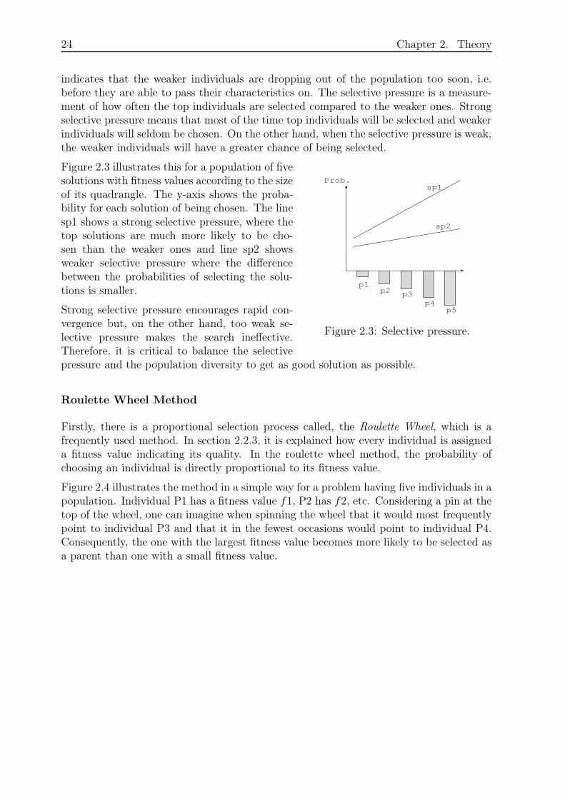
Figure 2.3 illustrates this for a population of fivesolutions with fitness values according to the sizeof its quadrangle. The y-axis shows the proba-bility for each solution of being chosen. The linesp1 shows a strong selective pressure, where thetop solutions are much more likely to be cho-sen than the weaker ones and line sp2 showsweaker selective pressure where the differencebetween the probabilities of selecting the solu-tions is smaller.
Strong selective pressure encourages rapid con-vergence but, on the other hand, too weak se-lective pressure makes the search ineffective.Therefore, it is critical to balance the selectivepressure and the population diversity to get as good solution as possible.
Roulette Wheel Method
Firstly, there is a proportional selection process called, the Roulette Wheel, which is afrequently used method. In section 2.2.3, it is explained how every individual is assigneda fitness value indicating its quality. In the roulette wheel method, the probability ofchoosing an individual is directly proportional to its fitness value.
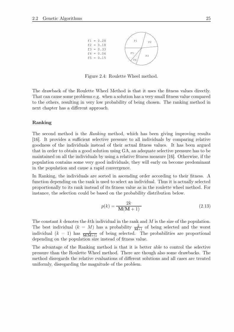
Figure 2.4 illustrates the method in a simple way for a problem having five individuals in apopulation. Individual P1 has a fitness value f1, P2 has f2, etc. Considering a pin at thetop of the wheel, one can imagine when spinning the wheel that it would most frequentlypoint to individual P3 and that it in the fewest occasions would point to individual P4.Consequently, the one with the largest fitness value becomes more likely to be selected asa parent than one with a small fitness value.
2.2 Genetic Algorithms 25
P1
P5
P4
P3
P2
f3 = 0.33f4 = 0.06f5 = 0.15
f1 = 0.28f2 = 0.18
Figure 2.4: Roulette Wheel method.
The drawback of the Roulette Wheel Method is that it uses the fitness values directly.That can cause some problems e.g. when a solution has a very small fitness value comparedto the others, resulting in very low probability of being chosen. The ranking method innext chapter has a different approach.
Ranking
The second method is the Ranking method, which has been giving improving results[16]. It provides a sufficient selective pressure to all individuals by comparing relativegoodness of the individuals instead of their actual fitness values. It has been arguedthat in order to obtain a good solution using GA, an adequate selective pressure has to bemaintained on all the individuals by using a relative fitness measure [16]. Otherwise, if thepopulation contains some very good individuals, they will early on become predominantin the population and cause a rapid convergence.
In Ranking, the individuals are sorted in ascending order according to their fitness. Afunction depending on the rank is used to select an individual. Thus it is actually selectedproportionally to its rank instead of its fitness value as in the roulette wheel method. Forinstance, the selection could be based on the probability distribution below.
p(k) =2k
M(M + 1)(2.13)
The constant k denotes the kth individual in the rank and M is the size of the population.The best individual (k = M) has a probability 2
M+1of being selected and the worst
individual (k = 1) has 2M(M+1)
of being selected. The probabilities are proportionaldepending on the population size instead of fitness value.
The advantage of the Ranking method is that it is better able to control the selectivepressure than the Roulette Wheel method. There are though also some drawbacks. Themethod disregards the relative evaluations of different solutions and all cases are treateduniformly, disregarding the magnitude of the problem.
26 Chapter 2. Theory
Tournament Selection
The Tournament Selection is an efficient combination of selection and ranking methods.A parent is selected by choosing the best individual from a set of individuals or a subgroupfrom the population. The steady-state algorithm on page 21 requires only two individualsfor each parent in every iteration and a third one to be replaced by the offspring at theend of the iteration. The method is explained considering the steady-state algorithm.
At first, two subgroups of each S individuals are randomly selected, since two parents areneeded. If k individuals of the population were changed in each iteration, the number ofsubgroups would be k. Each subgroup must contain at least two individuals, to enable acomparison between them. The size of the subgroups influences the selective pressure, i.e.more individuals in the subgroups increase the selection pressure on the better individuals.Within each subgroup, the individuals compete for selection like in a tournament. Whenselecting individuals for reproduction the best individual within each subgroup is selected.On the other hand, the worst individual is chosen when the method is used to select aindividual to leave the population. Then the worst individual will not be selected forreproduction and more importantly the best individual will never leave the population.
The Tournament Selection is the selection method that will be used in this project for bothselection of individuals for reproduction and surviving. It combines the characteristics ofthe Roulette Wheel and the Ranking Method and is without the drawbacks of thesemethods have.
2.2.5 Crossover
The main genetic operator is crossover, which simulates a reproduction between twoorganisms, the parents. It works on a pair of solutions and recombines them in a certainway generating one or more offsprings. The offsprings share some of the characteristicsof the parents and in that way the characteristic are passed on to the future generations.It is not able to produce new characteristics.
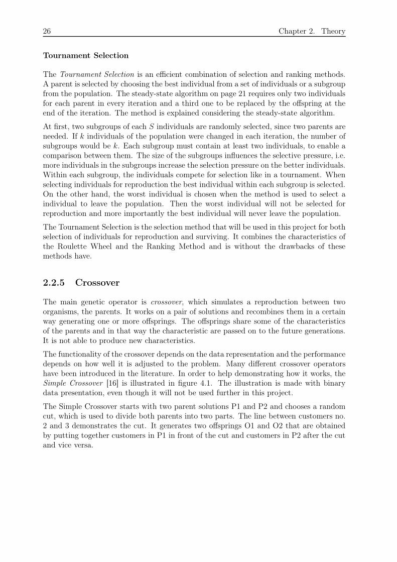
The functionality of the crossover depends on the data representation and the performancedepends on how well it is adjusted to the problem. Many different crossover operatorshave been introduced in the literature. In order to help demonstrating how it works, theSimple Crossover [16] is illustrated in figure 4.1. The illustration is made with binarydata presentation, even though it will not be used further in this project.
The Simple Crossover starts with two parent solutions P1 and P2 and chooses a randomcut, which is used to divide both parents into two parts. The line between customers no.2 and 3 demonstrates the cut. It generates two offsprings O1 and O2 that are obtainedby putting together customers in P1 in front of the cut and customers in P2 after the cutand vice versa.
2.2 Genetic Algorithms 27
1 0 11
0111 1
10
1
P1:
P2:
1 1 11 10 1 0 01 11O2:O1:
Figure 2.5: Illustration of Simple Crossover. The offspring O1 is generated from the righthalf of P1 and the left half of P2 and O2 is made from the left half of P1 and the righthalf of P2.
2.2.6 Mutation
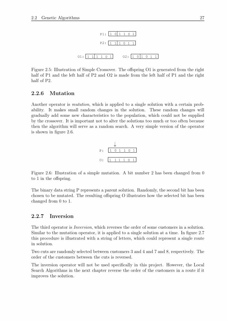
Another operator is mutation, which is applied to a single solution with a certain prob-ability. It makes small random changes in the solution. These random changes willgradually add some new characteristics to the population, which could not be suppliedby the crossover. It is important not to alter the solutions too much or too often becausethen the algorithm will serve as a random search. A very simple version of the operatoris shown in figure 2.6.
1 0 11 10P:
1 1 11 10O:
Figure 2.6: Illustration of a simple mutation. A bit number 2 has been changed from 0to 1 in the offspring.
The binary data string P represents a parent solution. Randomly, the second bit has beenchosen to be mutated. The resulting offspring O illustrates how the selected bit has beenchanged from 0 to 1.
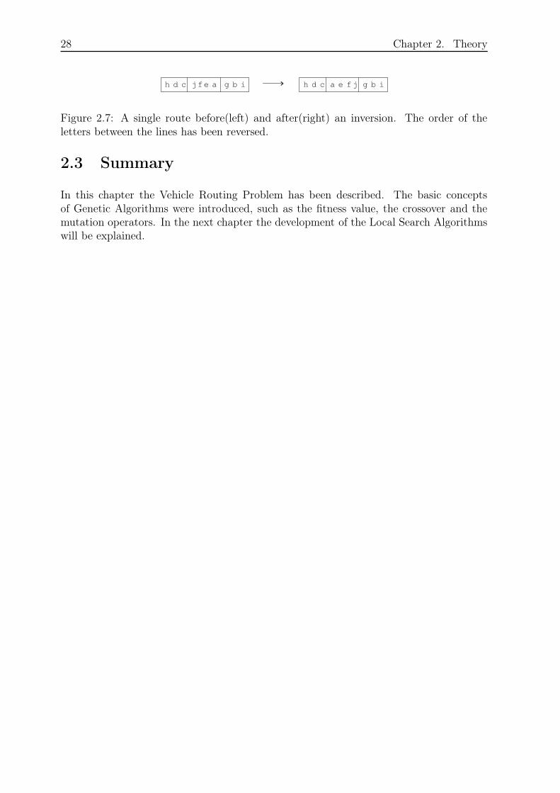
2.2.7 Inversion
The third operator is Inversion, which reverses the order of some customers in a solution.Similar to the mutation operator, it is applied to a single solution at a time. In figure 2.7this procedure is illustrated with a string of letters, which could represent a single routein solution.
Two cuts are randomly selected between customers 3 and 4 and 7 and 8, respectively. Theorder of the customers between the cuts is reversed.
The inversion operator will not be used specifically in this project. However, the LocalSearch Algorithms in the next chapter reverse the order of the customers in a route if itimproves the solution.
28 Chapter 2. Theory
aefjh d c g b i jfeah d c g b i
Figure 2.7: A single route before(left) and after(right) an inversion. The order of theletters between the lines has been reversed.
2.3 Summary
In this chapter the Vehicle Routing Problem has been described. The basic conceptsof Genetic Algorithms were introduced, such as the fitness value, the crossover and themutation operators. In the next chapter the development of the Local Search Algorithmswill be explained.
29
Chapter 3
Local Search Algorithms
The experience of the last few years has shown that combining Genetic Algorithms withLocal Search Algorithms (LSA) is necessary to be able to solve VRP effectively [10]. TheLSA can be used to improve VRP solutions in two ways. They can either be improvementheuristics for TSP that are applied to only one route at a time or multi-route improvementmethods that exploit the route structure of a whole solution [13]. In this project, LSAwill only be used to improve a single route at a time.
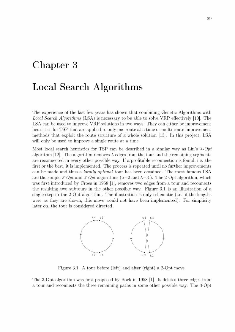
Most local search heuristics for TSP can be described in a similar way as Lin’s λ-Optalgorithm [12]. The algorithm removes λ edges from the tour and the remaining segmentsare reconnected in every other possible way. If a profitable reconnection is found, i.e. thefirst or the best, it is implemented. The process is repeated until no further improvementscan be made and thus a locally optimal tour has been obtained. The most famous LSAare the simple 2-Opt and 3-Opt algorithms (λ=2 and λ=3 ). The 2-Opt algorithm, whichwas first introduced by Croes in 1958 [1], removes two edges from a tour and reconnectsthe resulting two subtours in the other possible way. Figure 3.1 is an illustration of asingle step in the 2-Opt algorithm. The illustration is only schematic (i.e. if the lengthswere as they are shown, this move would not have been implemented). For simplicitylater on, the tour is considered directed.
t4
t1t2
t3 t4
t1t2
t3
Figure 3.1: A tour before (left) and after (right) a 2-Opt move.
The 3-Opt algorithm was first proposed by Bock in 1958 [1]. It deletes three edges froma tour and reconnects the three remaining paths in some other possible way. The 3-Opt
30 Chapter 3. Local Search Algorithms
algorithm is not implemented here because it is not likely to pay off. This is shown in [1]where test results propose that for problems of 100 customers the performance of 3-Optis only 2% better than 2-Opt. The biggest VRP that will be solved in this project has262 customers and minimum 25 vehicles (see chapter 7) thus each route will most likelyhave considerably fewer customers than 100. Therefore, the difference in performance canbe assumed to be even less. Furthermore, 3-Opt is more time consuming and difficult toimplement.
There are different ways to make both 2-Opt and 3-Opt run faster. For instance byimplementing a neighbour-list, which stores the k nearest neighbours for each customer[1]. As an example, consider a chosen t1 and t2. The number of possible candidates fort3 (see figure 3.1) is reduced to k instead of n − 3 where n is the number of customersin the route. However, since the algorithm will be applied to rather short routes, aswas explained above, it will most likely not pay off. The emphasis will be on producingrather simple but effective and 2-Opt algorithms. The 2-Opt algorithm is very sensitiveto the sequence in which moves are performed [11]. Considering the sequence of movesthree different 2-Opt algorithms have been put forward. In the following sections theyare explained and compared. The best one will be used along in the process.
3.1 Simple Random Algorithm
The Simple Random Algorithm (SRA) is the most simple 2-Opt algorithm explained inthis chapter. It starts by randomly selecting a customer t1 from a given tour, which isthe starting point of the first edge to be removed. Then it searches through all possiblecustomers for the second edge to be removed giving the largest possible improvement. Itis not possible to remove two edges that are next to each other, because that will onlyresult in exactly the same tour again. If an improvement is found, the sequence of thecustomers in the tour is rearranged according to figure 3.1. The process is repeated untilno further improvement is possible.
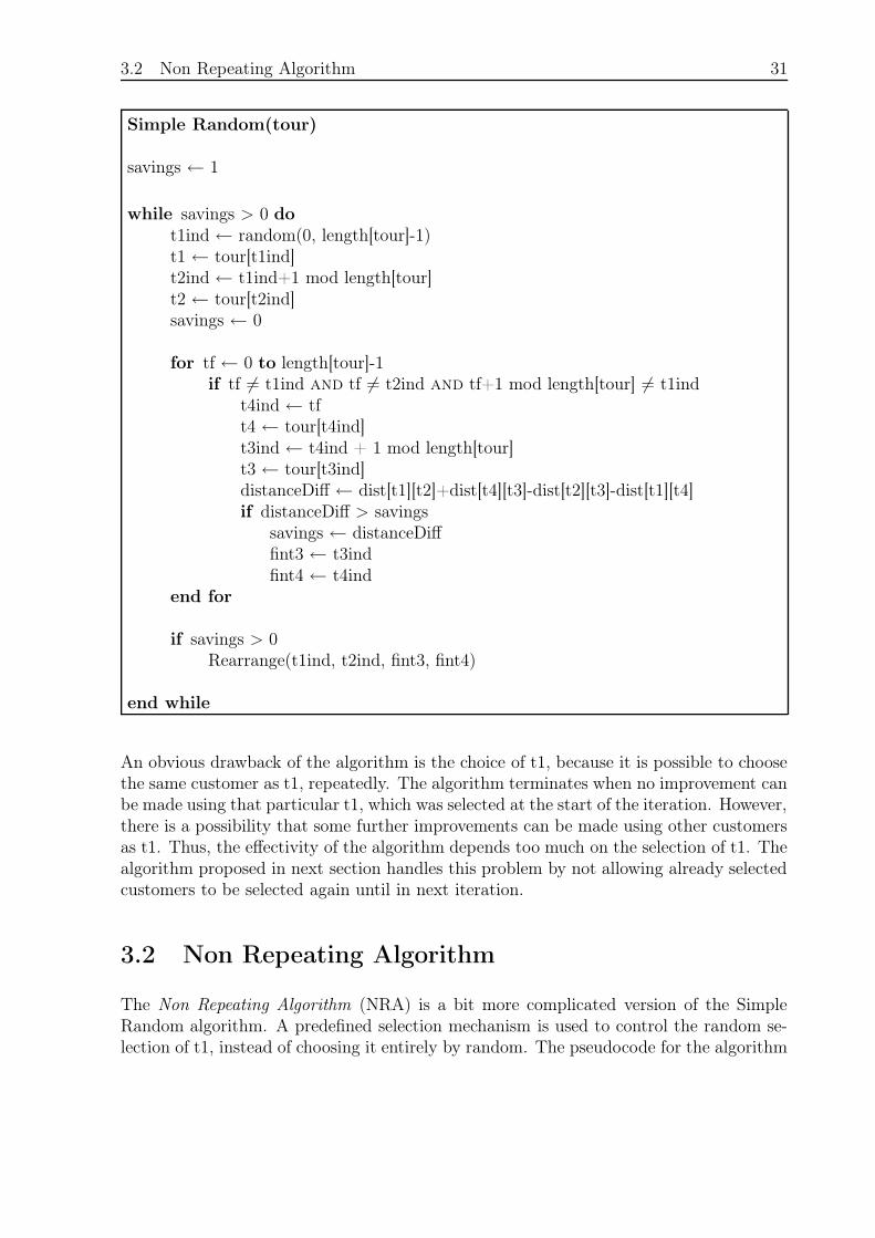
3.2 Non Repeating Algorithm 31
Simple Random(tour)
savings ← 1
while savings > 0 dot1ind ← random(0, length[tour]-1)t1 ← tour[t1ind]t2ind ← t1ind+1 mod length[tour]t2 ← tour[t2ind]savings ← 0
for tf ← 0 to length[tour]-1if tf 6= t1ind and tf 6= t2ind and tf+1 mod length[tour] 6= t1ind
t4ind ← tft4 ← tour[t4ind]t3ind ← t4ind + 1 mod length[tour]t3 ← tour[t3ind]distanceDiff ← dist[t1][t2]+dist[t4][t3]-dist[t2][t3]-dist[t1][t4]if distanceDiff > savings
savings ← distanceDifffint3 ← t3indfint4 ← t4ind
end for
if savings > 0Rearrange(t1ind, t2ind, fint3, fint4)
end while
An obvious drawback of the algorithm is the choice of t1, because it is possible to choosethe same customer as t1, repeatedly. The algorithm terminates when no improvement canbe made using that particular t1, which was selected at the start of the iteration. However,there is a possibility that some further improvements can be made using other customersas t1. Thus, the effectivity of the algorithm depends too much on the selection of t1. Thealgorithm proposed in next section handles this problem by not allowing already selectedcustomers to be selected again until in next iteration.
3.2 Non Repeating Algorithm
The Non Repeating Algorithm (NRA) is a bit more complicated version of the SimpleRandom algorithm. A predefined selection mechanism is used to control the random se-lection of t1, instead of choosing it entirely by random. The pseudocode for the algorithm
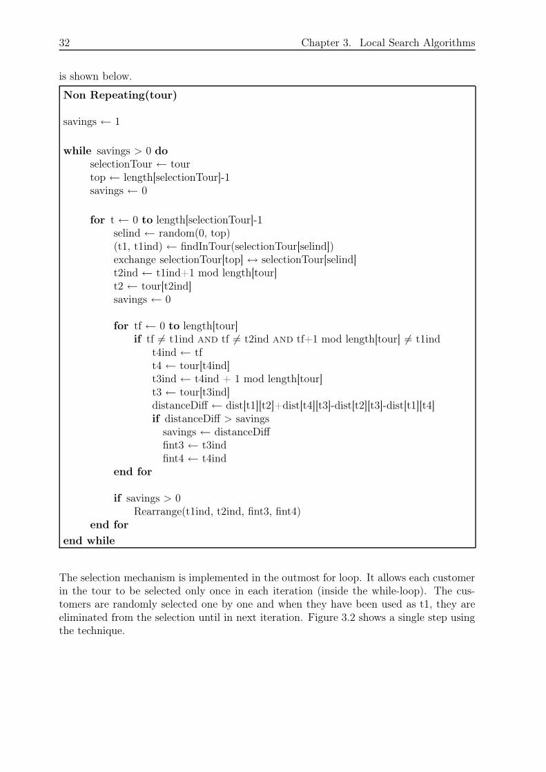
32 Chapter 3. Local Search Algorithms
is shown below.
Non Repeating(tour)
savings ← 1
while savings > 0 doselectionTour ← tourtop ← length[selectionTour]-1savings ← 0
for t ← 0 to length[selectionTour]-1selind ← random(0, top)(t1, t1ind) ← findInTour(selectionTour[selind])exchange selectionTour[top] ↔ selectionTour[selind]t2ind ← t1ind+1 mod length[tour]t2 ← tour[t2ind]savings ← 0
for tf ← 0 to length[tour]if tf 6= t1ind and tf 6= t2ind and tf+1 mod length[tour] 6= t1ind
t4ind ← tft4 ← tour[t4ind]t3ind ← t4ind + 1 mod length[tour]t3 ← tour[t3ind]distanceDiff ← dist[t1][t2]+dist[t4][t3]-dist[t2][t3]-dist[t1][t4]if distanceDiff > savings
savings ← distanceDifffint3 ← t3indfint4 ← t4ind
end for
if savings > 0Rearrange(t1ind, t2ind, fint3, fint4)
end for
end while
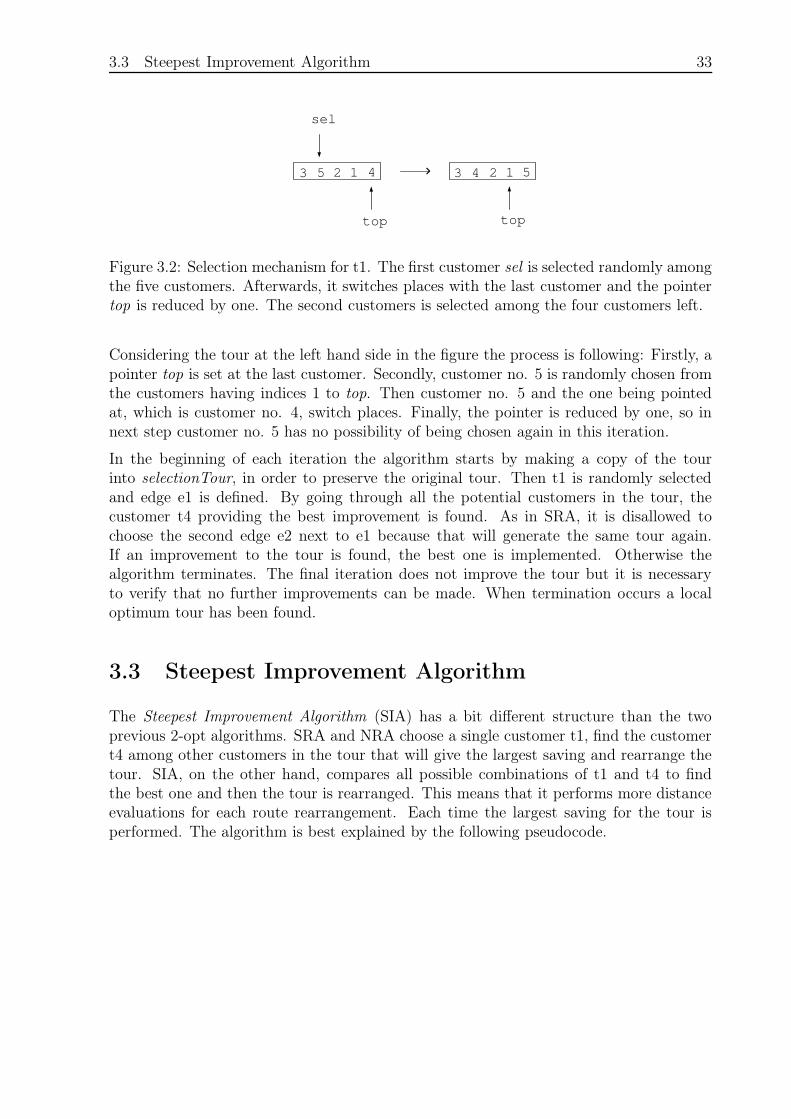
The selection mechanism is implemented in the outmost for loop. It allows each customerin the tour to be selected only once in each iteration (inside the while-loop). The cus-tomers are randomly selected one by one and when they have been used as t1, they areeliminated from the selection until in next iteration. Figure 3.2 shows a single step usingthe technique.
3.3 Steepest Improvement Algorithm 33
3 5 2 1 4 3 4 2 1 5
top
sel
top
Figure 3.2: Selection mechanism for t1. The first customer sel is selected randomly amongthe five customers. Afterwards, it switches places with the last customer and the pointertop is reduced by one. The second customers is selected among the four customers left.
Considering the tour at the left hand side in the figure the process is following: Firstly, apointer top is set at the last customer. Secondly, customer no. 5 is randomly chosen fromthe customers having indices 1 to top. Then customer no. 5 and the one being pointedat, which is customer no. 4, switch places. Finally, the pointer is reduced by one, so innext step customer no. 5 has no possibility of being chosen again in this iteration.
In the beginning of each iteration the algorithm starts by making a copy of the tourinto selectionTour, in order to preserve the original tour. Then t1 is randomly selectedand edge e1 is defined. By going through all the potential customers in the tour, thecustomer t4 providing the best improvement is found. As in SRA, it is disallowed tochoose the second edge e2 next to e1 because that will generate the same tour again.If an improvement to the tour is found, the best one is implemented. Otherwise thealgorithm terminates. The final iteration does not improve the tour but it is necessaryto verify that no further improvements can be made. When termination occurs a localoptimum tour has been found.
3.3 Steepest Improvement Algorithm
The Steepest Improvement Algorithm (SIA) has a bit different structure than the twoprevious 2-opt algorithms. SRA and NRA choose a single customer t1, find the customert4 among other customers in the tour that will give the largest saving and rearrange thetour. SIA, on the other hand, compares all possible combinations of t1 and t4 to findthe best one and then the tour is rearranged. This means that it performs more distanceevaluations for each route rearrangement. Each time the largest saving for the tour isperformed. The algorithm is best explained by the following pseudocode.
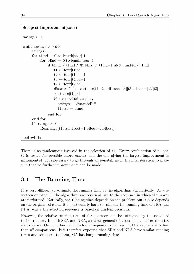
34 Chapter 3. Local Search Algorithms
Steepest Improvement(tour)
savings ← 1
while savings > 0 dosavings ← 0for t1ind ← 0 to length[tour]-1
for t4ind ← 0 to length[tour]-1if t4ind 6= t1ind and t4ind 6= t1ind+1 and t4ind+16= t1ind
t1 ← tour[t1ind]t2 ← tour[t1ind+1]t3 ← tour[t4ind+1]t4 ← tour[t4ind]distanceDiff ← distance[t1][t2]+distance[t4][t3]-distance[t2][t3]-distance[t1][t4]
if distanceDiff>savingssavings ← distanceDifft1best ← t1ind
end forend forif savings > 0
Rearrange(t1best,t1best+1,t4best+1,t4best)
end while
There is no randomness involved in the selection of t1. Every combination of t1 andt4 is tested for possible improvements and the one giving the largest improvement isimplemented. It is necessary to go through all possibilities in the final iteration to makesure that no further improvements can be made.
3.4 The Running Time
It is very difficult to estimate the running time of the algorithms theoretically. As waswritten on page 30, the algorithms are very sensitive to the sequence in which the movesare performed. Naturally, the running time depends on the problem but it also dependson the original solution. It is particularly hard to estimate the running time of SRA andNRA, where the selection sequence is based on random decisions.
However, the relative running time of the operators can be estimated by the means oftheir structure. In both SRA and NRA, a rearrangement of a tour is made after almost ncomparisons. On the other hand, each rearrangement of a tour in SIA requires a little lessthan n2 comparisons. It is therefore expected that SRA and NRA have similar runningtimes and compared to them, SIA has longer running time.
3.5 Comparison 35
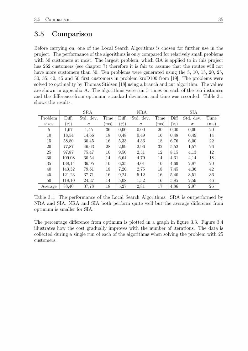
3.5 Comparison
Before carrying on, one of the Local Search Algorithms is chosen for further use in theproject. The performance of the algorithms is only compared for relatively small problemswith 50 customers at most. The largest problem, which GA is applied to in this projecthas 262 customers (see chapter 7) therefore it is fair to assume that the routes will nothave more customers than 50. Ten problems were generated using the 5, 10, 15, 20, 25,30, 35, 40, 45 and 50 first customers in problem kroD100 from [19]. The problems weresolved to optimality by Thomas Stidsen [18] using a branch and cut algorithm. The valuesare shown in appendix A. The algorithms were run 5 times on each of the ten instancesand the difference from optimum, standard deviation and time was recorded. Table 3.1shows the results.
SRA NRA SIA
Problem Diff. Std. dev. Time Diff. Std. dev. Time Diff Std. dev. Timesizes (%) σ (ms) (%) σ (ms) (%) σ (ms)
5 1,67 1,45 36 0,00 0,00 20 0,00 0,00 2010 18,54 14,66 18 0,48 0,49 16 0,48 0,49 1415 58,80 30,45 16 5,33 4,36 18 6,76 6,00 2220 77,87 46,63 28 2,99 2,96 32 5,52 1,57 2625 97,87 75,47 10 9,50 2,31 12 8,15 4,13 1230 109,08 30,54 14 6,64 4,79 14 4,31 4,14 1835 138,14 36,95 10 6,25 4,01 10 4,69 2,87 2040 143,32 79,61 18 7,20 2,75 18 7,45 4,36 4245 121,23 37,71 16 9,24 5,12 16 5,40 3,51 3650 118,10 24,37 14 5,08 1,32 16 5,85 2,59 46
Average 88,40 37,78 18 5,27 2,81 17 4,86 2,97 26
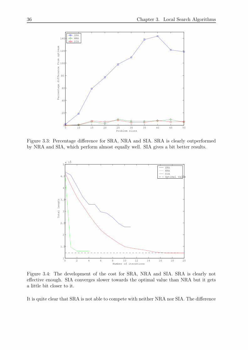
Table 3.1: The performance of the Local Search Algorithms. SRA is outperformed byNRA and SIA. NRA and SIA both perform quite well but the average difference fromoptimum is smaller for SIA.
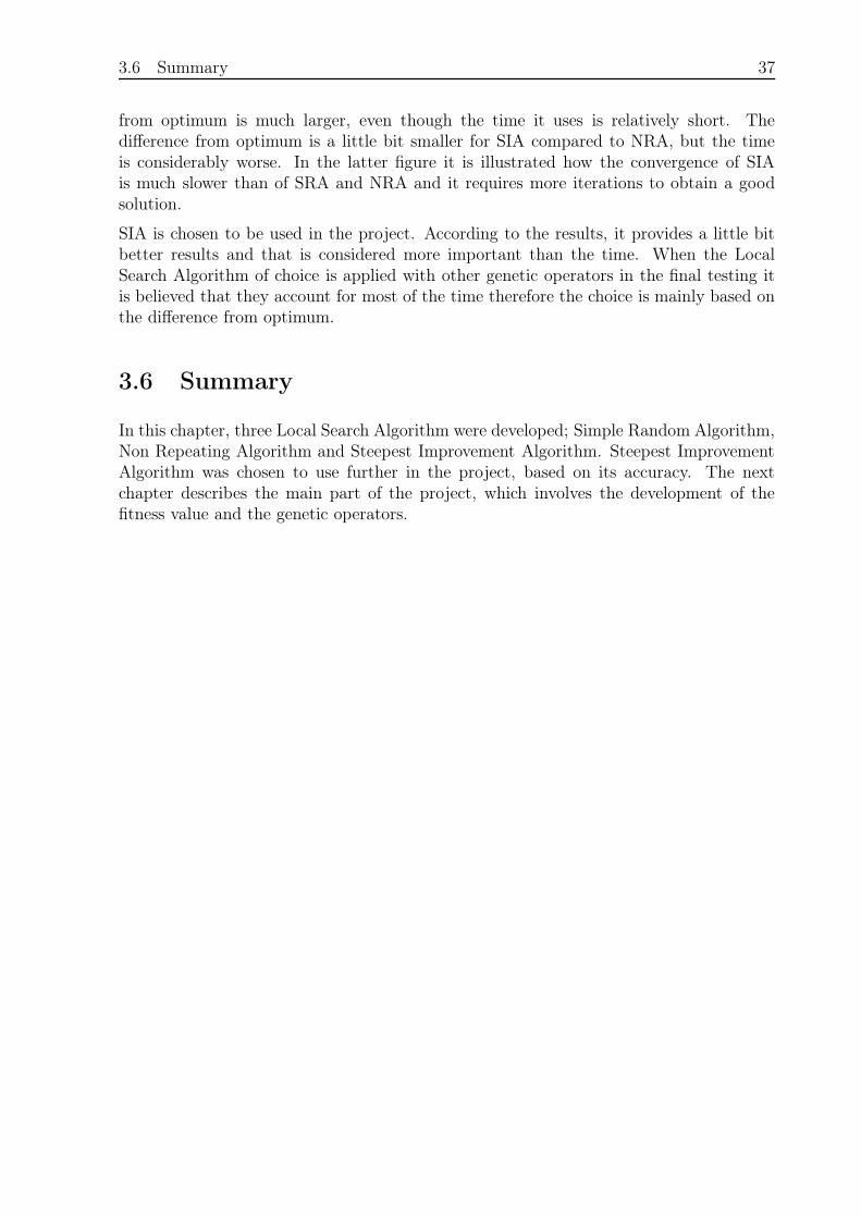
The percentage difference from optimum is plotted in a graph in figure 3.3. Figure 3.4illustrates how the cost gradually improves with the number of iterations. The data iscollected during a single run of each of the algorithms when solving the problem with 25customers.
36 Chapter 3. Local Search Algorithms
5 10 15 20 25 30 35 40 45 500
20
40
60
80
100
120
140
Problem sizes
Percentage difference from optimum
SRANRASIA
Figure 3.3: Percentage difference for SRA, NRA and SIA. SRA is clearly outperformedby NRA and SIA, which perform almost equally well. SIA gives a bit better results.
0 2 4 6 8 10 12 14 16 18 201
1.5
2
2.5
3
3.5
4
4.5
5x 10
4
Number of iterations
Total length
SRANRASIAOptimal value
Figure 3.4: The development of the cost for SRA, NRA and SIA. SRA is clearly noteffective enough. SIA converges slower towards the optimal value than NRA but it getsa little bit closer to it.
It is quite clear that SRA is not able to compete with neither NRA nor SIA. The difference
3.6 Summary 37
from optimum is much larger, even though the time it uses is relatively short. Thedifference from optimum is a little bit smaller for SIA compared to NRA, but the timeis considerably worse. In the latter figure it is illustrated how the convergence of SIAis much slower than of SRA and NRA and it requires more iterations to obtain a goodsolution.
SIA is chosen to be used in the project. According to the results, it provides a little bitbetter results and that is considered more important than the time. When the LocalSearch Algorithm of choice is applied with other genetic operators in the final testing itis believed that they account for most of the time therefore the choice is mainly based onthe difference from optimum.
3.6 Summary
In this chapter, three Local Search Algorithm were developed; Simple Random Algorithm,Non Repeating Algorithm and Steepest Improvement Algorithm. Steepest ImprovementAlgorithm was chosen to use further in the project, based on its accuracy. The nextchapter describes the main part of the project, which involves the development of thefitness value and the genetic operators.

38 Chapter 3. Local Search Algorithms
39
Chapter 4
The Fitness Value and the Operators
The genetic operators and the evaluation function are among the basic items in GA (seepage 19). The operators can easily be adjusted to different problems and they need to becarefully designed in order to obtain an effective algorithm.
The geography of VRP plays an essential role when finding a good solution. By thegeography of a VRP it is referred to the relative position of the customers and the depot.Most of the operators that are explained in this chapter take this into consideration. Theexceptions are Simple Random Crossover and Simple Random Mutation, which dependexclusively on random choices. They were both adopted from the original project, seechapter 1. Some of the operators are able to generate infeasible solutions, with routesviolating the capacity constraint, thus the fitness value is designed to handle infeasiblesolutions.
Before the fitness value and the different operators are discussed, an overview of the mainissues of the development process is given.
Overview of the Development Process
1. The process began with designing three Local Search Algorithms that have alreadybeen explained and tested in chapter 3.
2. In the beginning, infeasible solutions were not allowed, even though the operatorswere capable of producing such solutions. Instead, the operators were applied re-peatedly until they produced a feasible solution and first then the offspring waschanged. That turned out to be a rather ineffective way to handle infeasible solu-tions. Instead the solution space was relaxed and a new fitness value was designedwith an additional penalty term depending on how much the vehicle capacity wasviolated. This is explained in the next section.
3. The Biggest Overlap Crossover (see section 4.2.2) was the first crossover operator tobe designed, since Simple Random Crossover was adopted from the previous project,see chapter 1. Experiments showed that both crossover operators were producing
40 Chapter 4. The Fitness Value and the Operators
offsprings that were far from being feasible, i.e. the total demand of the routes wasfar from being within the capacity limits. The Repairing Operator was generatedto carefully make the solutions less infeasible, see section 4.4.1.
4. The Horizontal Line Crossover (see section 4.2.3) gave a new approach that wassupposed to generate offsprings, which got their characteristics more equally fromboth parents. However, the offsprings turned out to have rather short routes andtoo many of them did not have enough similarity to their parents. GeographicalMerge was therefore designed to improve the offsprings by merging short routes.The Horizontal Line Crossover is discussed in section 4.2.3 and Geographical Mergeis considered in section 4.4.2.
5. Finally, Uniform Crossover was implemented. It was a further development of Hor-izontal Line Crossover, in order to try to increase the number of routes that weretransferred directly from the parent solutions. The operator is explained in section4.2.4.
4.1 The Fitness Value
Every solution has a fitness value assigned to it, which measures its quality. The theorybehind the fitness value is explained in section 2.2.3. In the beginning of the project,no infeasible solutions were allowed, i.e. solutions violating the capacity constraint, eventhough the operators were able to generate such solutions. To avoid infeasible solutionsthe operators were applied repeatedly until a feasible solution was obtained, which isinefficient and extremely time consuming. Thus, at first the fitness value was only ableto evaluate feasible VRP solutions.
It is rather straight forward to select a suitable fitness value for a VRP where the qualityof a solution s is based on the total cost of travelling for all vehicles;
fs =∑
r
costs,r (4.1)
where costs,r denotes the cost of route r in solution s.
Although it is the intention of GA to generate feasible solutions, it can often be profitableto allow infeasible solutions during the process. Expanding the search space over theinfeasible region does often enable the search for the optimal solution, particularly whendealing with non-convex feasible search spaces [16], as the search space of large VRP. Thefitness value was made capable of handling infeasible solutions by adding a penalty termdepending on how much the capacity constraint is violated. The penalty was supposed tobe insignificant at the early iterations, allowing infeasible solutions, and predominant inthe end to force the the final solution to be feasible. Experiments were needed to find theright fitness value that could balance the search between infeasible and feasible solutions.
4.1 The Fitness Value 41
It is reasonable to let the penalty function depend on the number of iterations, since itis supposed to develop with increasing number of iterations. The exponential functiondepending on the number of iteration exp(it) was tried, since it had just the right form.Unfortunately, in the early iterations the program ran into problems because of the sizeof the penalty term. The program is implemented in Java and the biggest number Javacan handle is approx. 92234 × 1018. Already in iteration 44, the penalty function grewbeyond those those limits (ln(92234 × 1018) = 43.6683). It also had the drawback thatis did not depend on the problem at all and it always grew equally fast no matter howmany iterations were supposed to be performed.
A new more sophisticated evaluation function for the fitness value was then developed.It is illustrated in equations 4.2 to 4.4.
fs =∑
r∈s
costs,r + α ·it
IT
∑
r∈s
(max(0, totdems,r − cap))2 (4.2)
α =best
1IT
(mnv2· cap)2
(4.3)
mnv =
⌈∑
c∈s demc
cap
⌉
(4.4)
where:
it is the current iteration,IT denotes the total number of iterations,totdemr,s is the total demand of route r in solution s,cap represents the uniform capacity of the vehicles,best is the total cost of the best solution in the beginning anddemc denotes the demand of customer c ∈ s.
The left part of the evaluation function is just the cost as in equation 4.1. It denotesthe fitness value of a feasible solution because the second part equals zero if the capacityconstraint is attained. The second part is the penalty term. The quantity of the violationof the capacity constraint is raised to the power of 2 and multiplied with a factor α and therelative number of iterations. By multiplying with it
ITthe penalty factor is dependent on
where in the process it is calculated, instead of the actual number of the current iteration.The factor α makes the penalty term problem dependent, because it includes the cost ofthe best solution in the initial population. It also converts the penalty term into the sameunits as the first part of the evaluation function has.
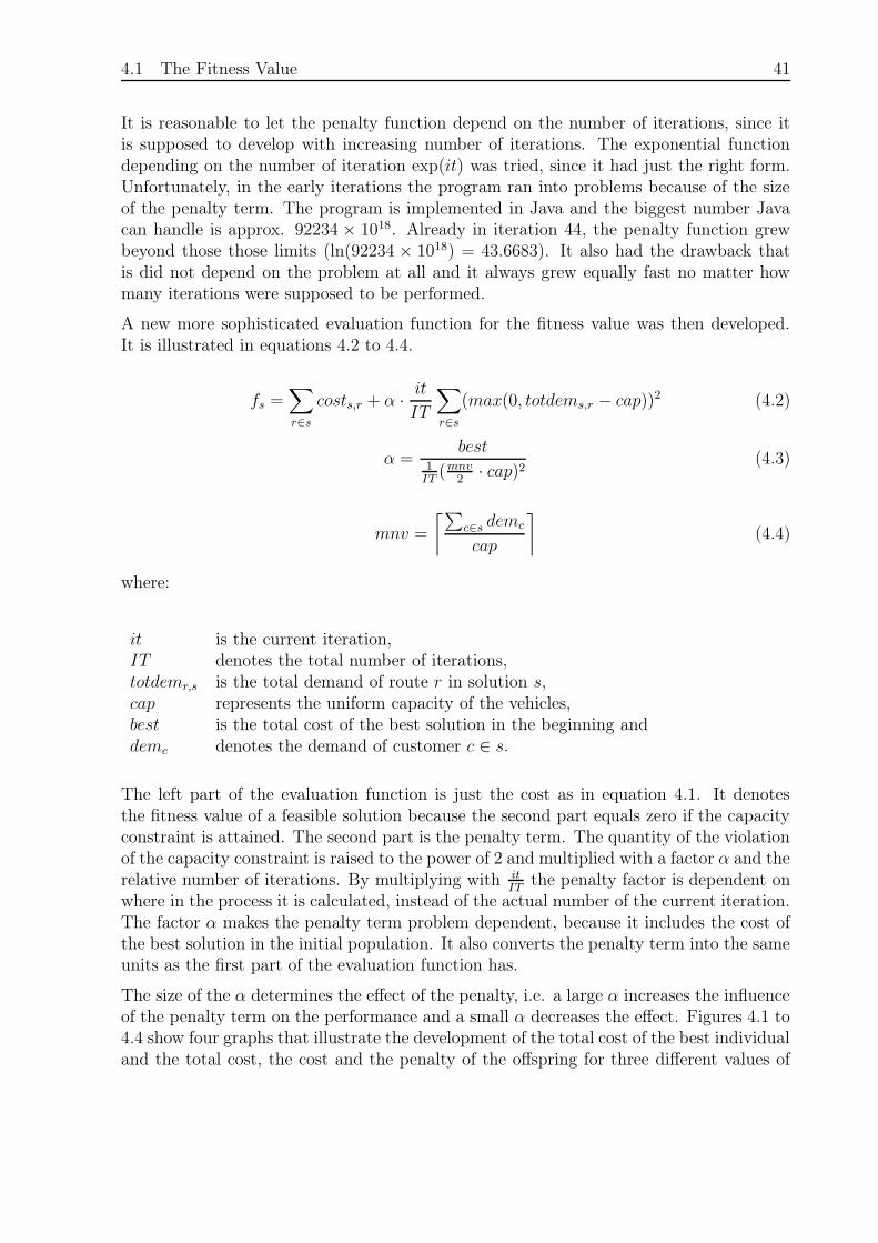
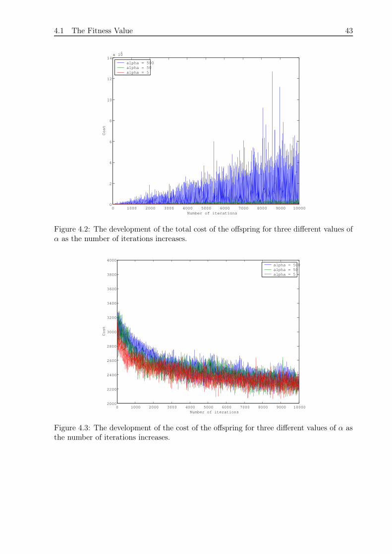
The size of the α determines the effect of the penalty, i.e. a large α increases the influenceof the penalty term on the performance and a small α decreases the effect. Figures 4.1 to4.4 show four graphs that illustrate the development of the total cost of the best individualand the total cost, the cost and the penalty of the offspring for three different values of
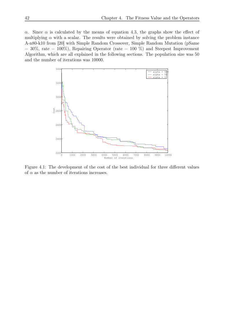
42 Chapter 4. The Fitness Value and the Operators
α. Since α is calculated by the means of equation 4.3, the graphs show the effect ofmultiplying α with a scalar. The results were obtained by solving the problem instanceA-n80-k10 from [20] with Simple Random Crossover, Simple Random Mutation (pSame= 30%, rate = 100%), Repairing Operator (rate = 100 %) and Steepest ImprovementAlgorithm, which are all explained in the following sections. The population size was 50and the number of iterations was 10000.
0 1000 2000 3000 4000 5000 6000 7000 8000 9000 100002200
2400
2600
2800
3000
3200
3400
Number of iterations
Cost
alpha = 500alpha = 50alpha = 5
Figure 4.1: The development of the cost of the best individual for three different valuesof α as the number of iterations increases.
4.1 The Fitness Value 43
0 1000 2000 3000 4000 5000 6000 7000 8000 9000 100000
2
4
6
8
10
12
14x 10
6
Number of iterations
Cost
alpha = 500alpha = 50alpha = 5
Figure 4.2: The development of the total cost of the offspring for three different values ofα as the number of iterations increases.
0 1000 2000 3000 4000 5000 6000 7000 8000 9000 100002000
2200
2400
2600
2800
3000
3200
3400
3600
3800
4000
Number of iterations
Cost
alpha = 500alpha = 50alpha = 5
Figure 4.3: The development of the cost of the offspring for three different values of α asthe number of iterations increases.
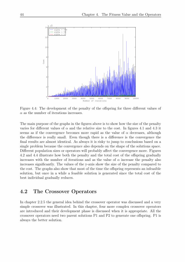
44 Chapter 4. The Fitness Value and the Operators
0 1000 2000 3000 4000 5000 6000 7000 8000 9000 100000
2
4
6
8
10
12
14x 10
6
Number of iterations
Cost
alpha = 500alpha = 50alpha = 5
Figure 4.4: The development of the penalty of the offspring for three different values ofα as the number of iterations increases.
The main purpose of the graphs in the figures above is to show how the size of the penaltyvaries for different values of α and the relative size to the cost. In figures 4.1 and 4.3 itseems as if the convergence becomes more rapid as the value of α decreases, althoughthe difference is really small. Even though there is a difference is the convergence thefinal results are almost identical. As always it is risky to jump to conclusions based on asingle problem because the convergence also depends on the shape of the solutions space.Different population sizes or operators will probably affect the convergence more. Figures4.2 and 4.4 illustrate how both the penalty and the total cost of the offspring graduallyincreases with the number of iterations and as the value of α increase the penalty alsoincreases significantly. The values of the y-axis show the size of the penalty compared tothe cost. The graphs also show that most of the time the offspring represents an infeasiblesolution, but once in a while a feasible solution is generated since the total cost of thebest individual gradually reduces.
4.2 The Crossover Operators
In chapter 2.2.5 the general idea behind the crossover operator was discussed and a verysimple crossover was illustrated. In this chapter, four more complex crossover operatorsare introduced and their development phase is discussed when it is appropriate. All thecrossover operators need two parent solutions P1 and P2 to generate one offspring. P1 isalways the better solution.
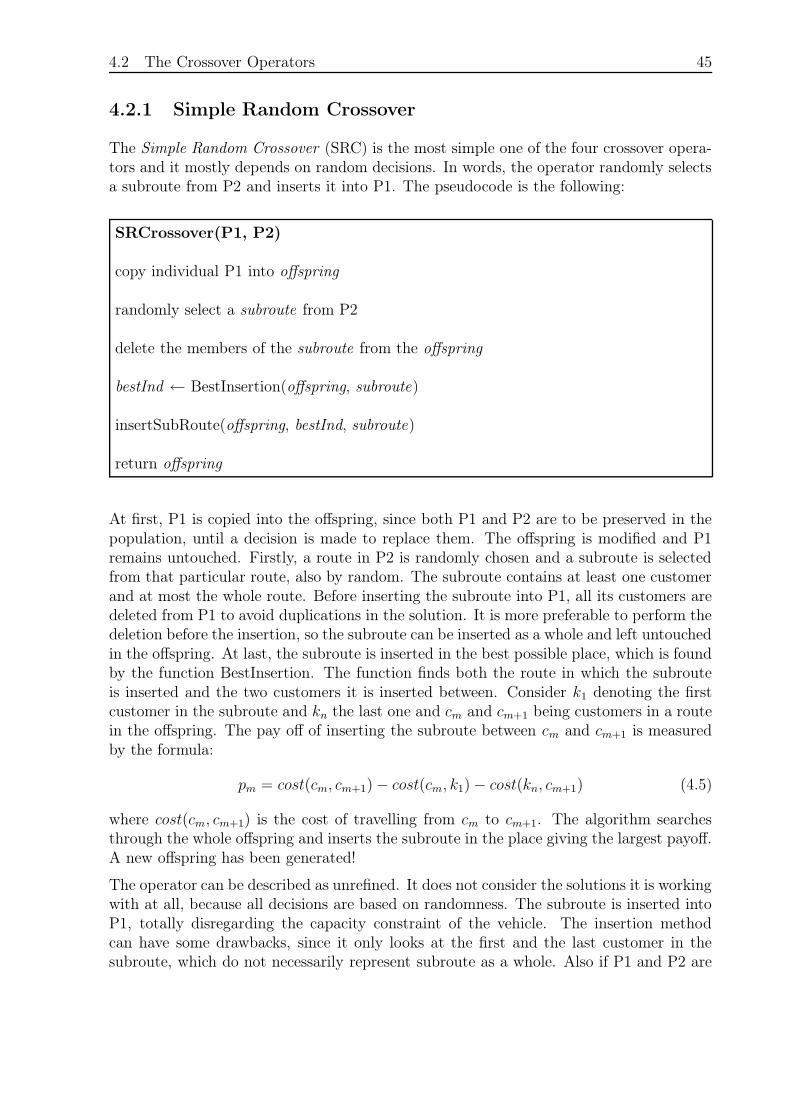
4.2 The Crossover Operators 45
4.2.1 Simple Random Crossover
The Simple Random Crossover (SRC) is the most simple one of the four crossover opera-tors and it mostly depends on random decisions. In words, the operator randomly selectsa subroute from P2 and inserts it into P1. The pseudocode is the following:
SRCrossover(P1, P2)
copy individual P1 into offspring
randomly select a subroute from P2
delete the members of the subroute from the offspring
bestInd ← BestInsertion(offspring, subroute)
insertSubRoute(offspring, bestInd, subroute)
return offspring
At first, P1 is copied into the offspring, since both P1 and P2 are to be preserved in thepopulation, until a decision is made to replace them. The offspring is modified and P1remains untouched. Firstly, a route in P2 is randomly chosen and a subroute is selectedfrom that particular route, also by random. The subroute contains at least one customerand at most the whole route. Before inserting the subroute into P1, all its customers aredeleted from P1 to avoid duplications in the solution. It is more preferable to perform thedeletion before the insertion, so the subroute can be inserted as a whole and left untouchedin the offspring. At last, the subroute is inserted in the best possible place, which is foundby the function BestInsertion. The function finds both the route in which the subrouteis inserted and the two customers it is inserted between. Consider k1 denoting the firstcustomer in the subroute and kn the last one and cm and cm+1 being customers in a routein the offspring. The pay off of inserting the subroute between cm and cm+1 is measuredby the formula:
pm = cost(cm, cm+1)− cost(cm, k1)− cost(kn, cm+1) (4.5)
where cost(cm, cm+1) is the cost of travelling from cm to cm+1. The algorithm searchesthrough the whole offspring and inserts the subroute in the place giving the largest payoff.A new offspring has been generated!
The operator can be described as unrefined. It does not consider the solutions it is workingwith at all, because all decisions are based on randomness. The subroute is inserted intoP1, totally disregarding the capacity constraint of the vehicle. The insertion methodcan have some drawbacks, since it only looks at the first and the last customer in thesubroute, which do not necessarily represent subroute as a whole. Also if P1 and P2 are
46 Chapter 4. The Fitness Value and the Operators
good solutions, they probably have almost or totally full vehicles on most of the routesand consequently the operator generates an infeasible solution. Since infeasible solutionsare penalised, it can make the algorithms ineffective if SRC generates infeasible solutionsmost of the time.
Furthermore, the geography of the problem is ignored. If the subroute is chosen from agood or partially good route the operator does not make any effort to choose the goodpart to pass on to the offspring. A totally random selection of a subroute can overlook itor just take a part of it. As a consequence, too much use of random selection can makeit difficult for good characteristics to spread out in the population. On the other hand,some randomness can be necessary to increase the diversity of the population.
In next chapter a crossover is introduced that compares the geography of the subroute tothe geography of the offspring when inserting the subroute into the offspring.
4.2.2 Biggest Overlap Crossover
The Biggest Overlap Crossover (BOC) can be looked at as an extended version of SRC. Ituses the geography of the solution, i.e. the relative position of the routes, in addition to thetotal demand of its routes, when inserting the subroute. Calculating the actual distancebetween every two routes can be complicated due to their different shapes. Therefore,so-called bounding boxes are used to measure the size of each route and to calculate thedistance between them. Further explanation of bounding boxes is given below.
As in SRC, the subroute is randomly selected from P1. There are two possible approachesof taking the geography or capacity into consideration. The first one, starts by choosingthree routes from P1 considering the size of the overlapping between the bounding boxesof the subroute and the routes of P1. The subroute is inserted into one of the three routeshaving the smallest total demand. The second approach first selects the three routeshaving the smallest total demand of the routes in P1, then the subroute is inserted intothe one of the three routes having the biggest overlap with the subroute. Both approachescan generate infeasible solutions, if the subroute contains customers with too large totaldemand. The two approaches that are called First Geography, then Capacity (GC) andFirst Capacity, then Geography (CG) are discussed further below and a comparison isgiven.
Bounding boxes
Each route has its own bounding box, which is the smallest quadrangle the entire routefits in (the depot is also a member of every route). Figure 4.5 illustrates the boundingboxes for a solution with four routes.
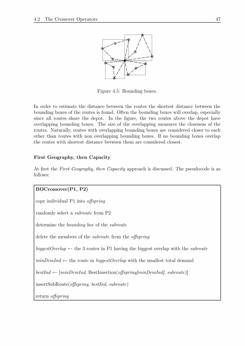
4.2 The Crossover Operators 47
Figure 4.5: Bounding boxes.
In order to estimate the distance between the routes the shortest distance between thebounding boxes of the routes is found. Often the bounding boxes will overlap, especiallysince all routes share the depot. In the figure, the two routes above the depot haveoverlapping bounding boxes. The size of the overlapping measures the closeness of theroutes. Naturally, routes with overlapping bounding boxes are considered closer to eachother than routes with non overlapping bounding boxes. If no bounding boxes overlapthe routes with shortest distance between them are considered closest.
First Geography, then Capacity
At first the First Geography, then Capacity approach is discussed. The pseudocode is asfollows:
BOCrossover(P1, P2)
copy individual P1 into offspring
randomly select a subroute from P2
determine the bounding box of the subroute
delete the members of the subroute from the offspring
biggestOverlap ← the 3 routes in P1 having the biggest overlap with the subroute
minDemInd ← the route in biggestOverlap with the smallest total demand
bestInd ← [minDemInd, BestInsertion(offspring[minDemInd], subroute)]
insertSubRoute(offspring, bestInd, subroute)
return offspring
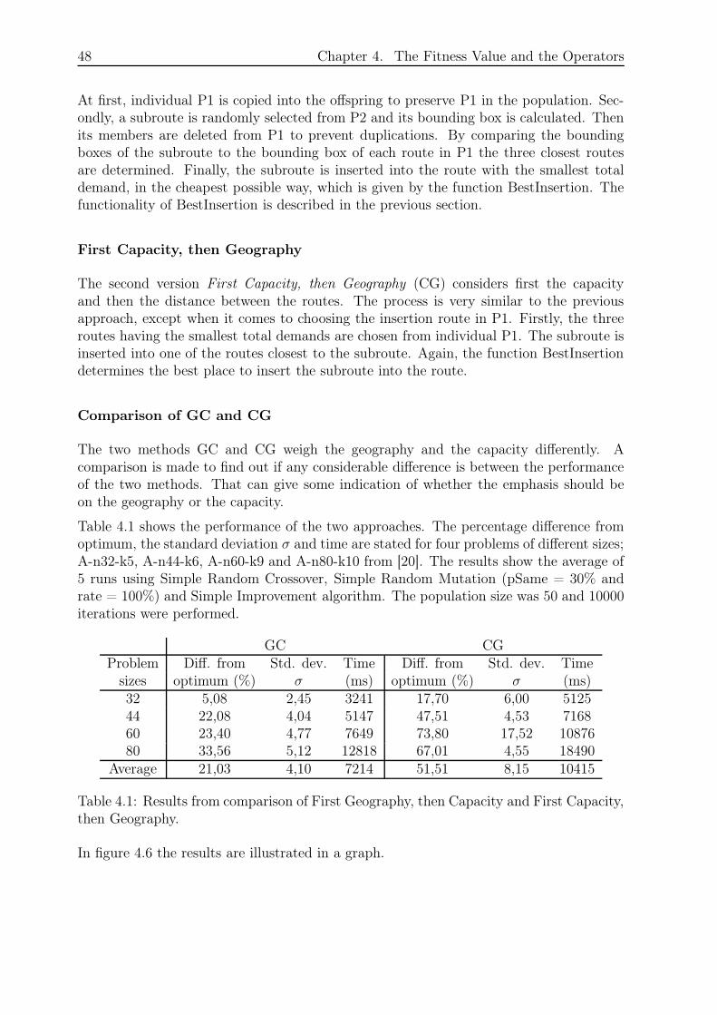
48 Chapter 4. The Fitness Value and the Operators
At first, individual P1 is copied into the offspring to preserve P1 in the population. Sec-ondly, a subroute is randomly selected from P2 and its bounding box is calculated. Thenits members are deleted from P1 to prevent duplications. By comparing the boundingboxes of the subroute to the bounding box of each route in P1 the three closest routesare determined. Finally, the subroute is inserted into the route with the smallest totaldemand, in the cheapest possible way, which is given by the function BestInsertion. Thefunctionality of BestInsertion is described in the previous section.
First Capacity, then Geography
The second version First Capacity, then Geography (CG) considers first the capacityand then the distance between the routes. The process is very similar to the previousapproach, except when it comes to choosing the insertion route in P1. Firstly, the threeroutes having the smallest total demands are chosen from individual P1. The subroute isinserted into one of the routes closest to the subroute. Again, the function BestInsertiondetermines the best place to insert the subroute into the route.
Comparison of GC and CG
The two methods GC and CG weigh the geography and the capacity differently. Acomparison is made to find out if any considerable difference is between the performanceof the two methods. That can give some indication of whether the emphasis should beon the geography or the capacity.
Table 4.1 shows the performance of the two approaches. The percentage difference fromoptimum, the standard deviation σ and time are stated for four problems of different sizes;A-n32-k5, A-n44-k6, A-n60-k9 and A-n80-k10 from [20]. The results show the average of5 runs using Simple Random Crossover, Simple Random Mutation (pSame = 30% andrate = 100%) and Simple Improvement algorithm. The population size was 50 and 10000iterations were performed.
GC CGProblem Diff. from Std. dev. Time Diff. from Std. dev. Time
sizes optimum (%) σ (ms) optimum (%) σ (ms)32 5,08 2,45 3241 17,70 6,00 512544 22,08 4,04 5147 47,51 4,53 716860 23,40 4,77 7649 73,80 17,52 1087680 33,56 5,12 12818 67,01 4,55 18490
Average 21,03 4,10 7214 51,51 8,15 10415
Table 4.1: Results from comparison of First Geography, then Capacity and First Capacity,then Geography.
In figure 4.6 the results are illustrated in a graph.
4.2 The Crossover Operators 49
30 35 40 45 50 55 60 65 70 75 800
10
20
30
40
50
60
70
80
Problem size
Percentage difference from optimum
capgeo geocap
Figure 4.6: Comparison of GC (geocap) and CG (capgeo). CG is definitely outperformedby GC.
The results are clear. For all four problem instances the deviation from optimum is atleast twice as large as for CG compared to GC. Besides, CG is more time consuming.Therefore, Biggest Overlap Crossover uses the GC approach in the rest of the project.
4.2.3 Horizontal Line Crossover
The Horizontal Line Crossover (HLC) introduces another method to generate offsprings.SRC and BOC generate offsprings that mostly come from P1, though it depends on therelative problem size to the vehicle capacity. The HLC tries to combine the solutionsP1 and P2 more equally in the offspring. A horizontal line is drawn through the depotand divides both solutions into two parts. Bounding boxes (see section 4.2.2) are usedto identify the routes. Routes in P1 having bounding boxes above the line are inserteduntouched into the offspring along with routes in P2 that have bounding boxes belowthe line. This is illustrated in figure 4.7. For simplification, the figure shows the routeswithout the bounding boxes but in figure 4.5 solution P2 is illustrated with boundingboxes.
50 Chapter 4. The Fitness Value and the Operators
P1 P2Offspring
+
Figure 4.7: An illustration of the Horizontal Line Crossover. Routes in P1 above the lineand route in P2 below the line are inserted untouched into the offspring. Note that therightmost customer is not a member.
The line has to be drawn through the depot, since all routes contain the depot. It couldalso be possible to draw the line vertically. However, the algorithm would not have beennear as effective if the line was drawn at an angle, since the bounding boxes are usedto identify the routes. That would reduce the number of routes that come directly fromthe parent solutions into the offspring. In the ideal case, no routes cross the line andall customers are transfered directly from the parent solutions to the offspring. This ishowever not always the case and in order to include all the customers in the offspringanother method is needed to gather the rest of the customers into the offspring. In figure4.7 the rightmost customer is not yet a member of any route in the offspring.
All classical heuristics that belong to the construction heuristics or the two-phase methodscan be used to generate new routes from the rest of the customers, see section 2.1.4. Thetwo-phase method the Sweep Algorithm is chosen here. The idea behind the SweepAlgorithm first came forward in the early 70ťs but generally it is attributed to Gillet andMiller that proposed it in 1974 [12]. In the first phase feasible routes are made by rotatinga ray centred at the depot and gradually it gathers the customers into clusters or routes.In the second phase a TSP is solved for each route. Here the Steepest ImprovementAlgorithm from chapter 3 is used to improve the routes where the initial order of thecustomers is the order in which they are gathered. It can therefore be expected that HLCdepends on Steepest Improvement Algorithm to provide good solutions.
The pseudocode is:
4.2 The Crossover Operators 51
HLCrossover(P1, P2)
NRP1 ← number of routes in P1NRP2 ← number of routes in P2offjind ← 0
for n ← 0 to NRP1if P1[n] is above a horizontal line through the depot
put route P1[n] into offspring [offjind]offjind ← offjind + 1
end for
for m ← 0 to NRP2if P2[m] is below a horizontal line through the depot
put route P2[m] into offspring [offjind]offjind ← offjind +1
end for
put all other customers into customersLeft
sweep the customers in customersLeft into feasible routes and put into the offspring
return offspring
In order to generate a good crossover, it is essential that the generated offsprings reflecton its parents. Therefore, it must be the aim of the crossover to pass as many routesas possible from the parent solutions to the offspring, thus leaving as few customers aspossible to the Sweep Algorithm. The disadvantage of HLC is that its quality depends onthe relative position of the customers to the depot. If the depot is placed relatively highor low in the graph, the routes will mainly be obtained from only one parent solution.Also, if many customers are placed around the line, it is expected that many routes crossthe line. Then too many customers will be put into the routes by the Sweep Algorithmand the crossover will basically become the Sweep Algorithm.
4.2.4 Uniform Crossover
The last type of crossover operator introduced is the Uniform Crossover (UC), whichis named after the Uniform Crossover known in the literature, e.g. in [16]. Considersolutions represented as binary strings, then for each bit the crossover chooses betweenthe bits in the parent solutions. In a similar way, UC chooses between the routes of theparent solutions based on the quality of the routes and as long as they do not conflictwith each other. The goal is to design a crossover that passes more routes directly fromthe parents, compared to the HLC in the previous section, and which performance does
52 Chapter 4. The Fitness Value and the Operators
not depend so much on the position of the depots.
In order to be able to explain the algorithm, a small problem of 13 customers is illustratedin figure 4.8. It shows two parent solutions of the problem and the cost of their routes.All routes in both these solutions attain the capacity constraint, so there is no penaltyinvolved in this case.
L1 = 16
L2 = 18
L3 = 14
L4 = 16
P1 P2
1
C
BA
3
2
D4
LA = 20
LB = 21
LC = 14
LD = 16
Figure 4.8: Two parent solutions and their route costs.
When solving VRP, the objective is to minimise the total cost of visiting all the customerswithout violating the vehicle capacity constraint, see chapter 2.1. Thus, it is desirable tohave the average cost of travelling between the customers in each route as low as possible.Therefore, the quotient Rs,r is calculated for each route r of every solution s and used tomeasure the quality of them.
Rs,r = totCosts,r/noCusts,r (4.6)
The term totCosts,r is the sum of the cost and penalty for route r in solution s andnoCusts,r denotes the number of customers in route r in solution s. The quotient for eachroute in the two solutions in figure 4.8 is:
P1 P2R1 = 8,0 RA = 5.0R2 = 6,0 RB = 7.0R3 = 4,7 RC = 4.7R4 = 3,2 RD = 5.3
Table 4.2: The quotient Rs,r for each route in figure 4.8.
The idea is now to transfer as many untouched routes from the parents to the offspring.However, it is not possible to move two routes from different individuals if they conflictwith each other, i.e. they share some customers. Each route in a solution will at leastconflict with one route in the other individual. In order to choose between those routes,the quotient Rs,r is used. The procedure is as follows; At first the route with the smallest
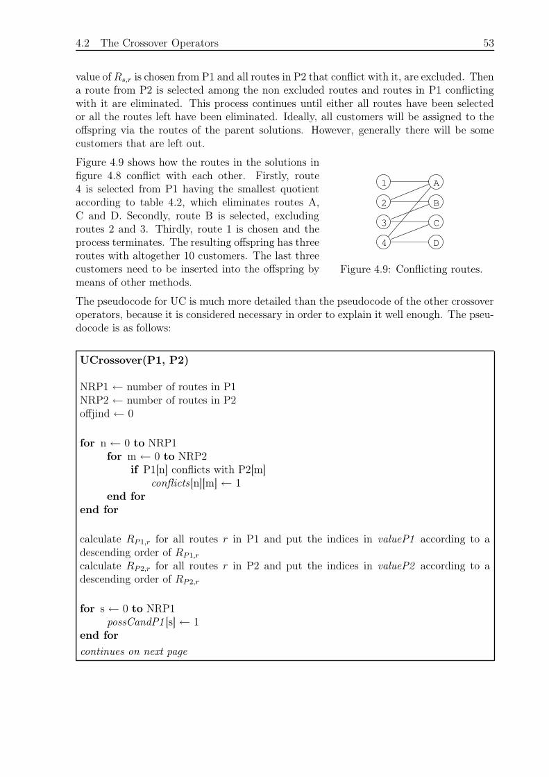
4.2 The Crossover Operators 53
value of Rs,r is chosen from P1 and all routes in P2 that conflict with it, are excluded. Thena route from P2 is selected among the non excluded routes and routes in P1 conflictingwith it are eliminated. This process continues until either all routes have been selectedor all the routes left have been eliminated. Ideally, all customers will be assigned to theoffspring via the routes of the parent solutions. However, generally there will be somecustomers that are left out.
1
3
2
D
C
B
A
4
Figure 4.9: Conflicting routes.
Figure 4.9 shows how the routes in the solutions infigure 4.8 conflict with each other. Firstly, route4 is selected from P1 having the smallest quotientaccording to table 4.2, which eliminates routes A,C and D. Secondly, route B is selected, excludingroutes 2 and 3. Thirdly, route 1 is chosen and theprocess terminates. The resulting offspring has threeroutes with altogether 10 customers. The last threecustomers need to be inserted into the offspring bymeans of other methods.
The pseudocode for UC is much more detailed than the pseudocode of the other crossoveroperators, because it is considered necessary in order to explain it well enough. The pseu-docode is as follows:
UCrossover(P1, P2)
NRP1 ← number of routes in P1NRP2 ← number of routes in P2offjind ← 0
for n ← 0 to NRP1for m ← 0 to NRP2
if P1[n] conflicts with P2[m]conflicts[n][m] ← 1
end forend for
calculate RP1,r for all routes r in P1 and put the indices in valueP1 according to adescending order of RP1,r
calculate RP2,r for all routes r in P2 and put the indices in valueP2 according to adescending order of RP2,r
for s ← 0 to NRP1possCandP1 [s] ← 1
end for
continues on next page
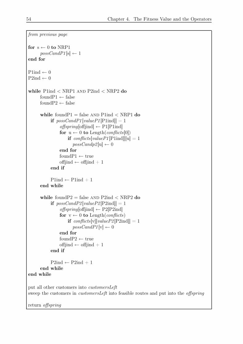
54 Chapter 4. The Fitness Value and the Operators
from previous page
for s ← 0 to NRP1possCandP1 [s] ← 1
end for
P1ind ← 0P2ind ← 0
while P1ind < NRP1 and P2ind < NRP2 dofoundP1 ← falsefoundP2 ← false
while foundP1 = false and P1ind < NRP1 doif possCandP1 [valueP1 [P1ind]] = 1
offspring [offjind] ← P1[P1ind]for u ← 0 to Length(conflicts[0])
if conflicts[valueP1 [P1ind]][u] = 1possCandp2 [u] ← 0
end forfoundP1 ← trueoffjind ← offjind + 1
end if
P1ind ← P1ind + 1end while
while foundP2 = false and P2ind < NRP2 doif possCandP2 [valueP2 [P2ind]] = 1
offspring [offjind] ← P2[P2ind]for v ← 0 to Length(conflicts)
if conflicts[v][valueP2 [P2ind]] = 1possCandP1 [v] ← 0
end forfoundP2 ← trueoffjind ← offjind + 1
end if
P2ind ← P2ind + 1end while
end while
put all other customers into customersLeftsweep the customers in customersLeft into feasible routes and put into the offspring
return offspring
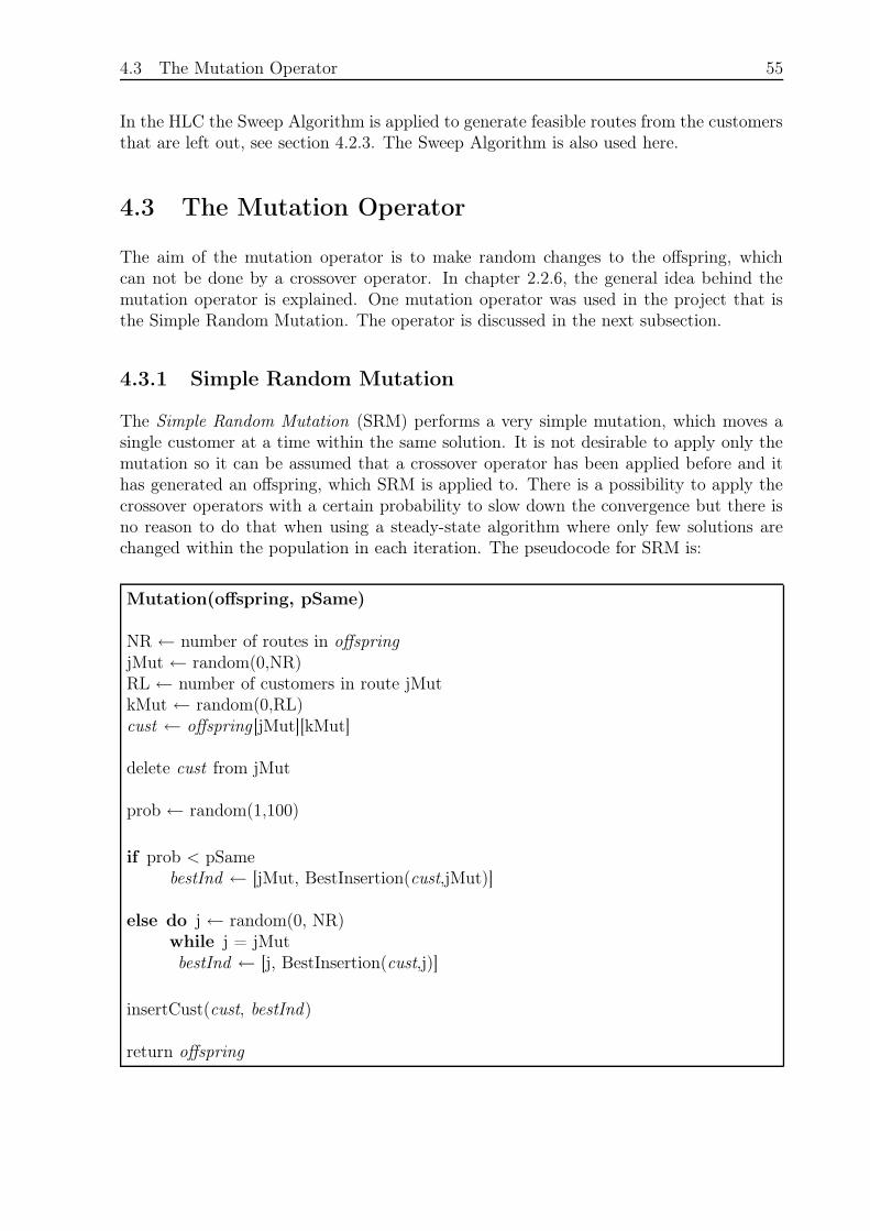
4.3 The Mutation Operator 55
In the HLC the Sweep Algorithm is applied to generate feasible routes from the customersthat are left out, see section 4.2.3. The Sweep Algorithm is also used here.
4.3 The Mutation Operator
The aim of the mutation operator is to make random changes to the offspring, whichcan not be done by a crossover operator. In chapter 2.2.6, the general idea behind themutation operator is explained. One mutation operator was used in the project that isthe Simple Random Mutation. The operator is discussed in the next subsection.
4.3.1 Simple Random Mutation
The Simple Random Mutation (SRM) performs a very simple mutation, which moves asingle customer at a time within the same solution. It is not desirable to apply only themutation so it can be assumed that a crossover operator has been applied before and ithas generated an offspring, which SRM is applied to. There is a possibility to apply thecrossover operators with a certain probability to slow down the convergence but there isno reason to do that when using a steady-state algorithm where only few solutions arechanged within the population in each iteration. The pseudocode for SRM is:
Mutation(offspring, pSame)
NR ← number of routes in offspringjMut ← random(0,NR)RL ← number of customers in route jMutkMut ← random(0,RL)cust ← offspring [jMut][kMut]
delete cust from jMut
prob ← random(1,100)
if prob < pSamebestInd ← [jMut, BestInsertion(cust,jMut)]
else do j ← random(0, NR)while j = jMutbestInd ← [j, BestInsertion(cust,j)]
insertCust(cust, bestInd)
return offspring
56 Chapter 4. The Fitness Value and the Operators
The operator starts by randomly selecting a route jMut in the offspring and then acustomer within the route is chosen randomly. The customer is deleted from the offspringto avoid duplication later on. It can either be inserted into the same route again or intoanother randomly chosen route within the same solution, controlled by the parameterpSame. The probability of being inserted into the same route again is equal to pSame.When the customer is inserted into the same route again, it is possible that it will beinserted in the same place as before and resulting in the same offspring again. Thefunction BestInsertion returns the index indicating the best place for the customer to beinserted. It measures the pay off in the same way as in SRC, see section 4.2.1, but theinsertion route has already been selected. The pay off of inserting customer k betweencustomers cm and cm+1 is:
pm = cost(cm, cm+1)− cost(cm, k)− cost(k, cm+1) (4.7)
where cost(cm, cm+1) is the cost of travelling between cm and cm+1.
It is important not to cause too much disruption using mutation, because that will ruinthe characteristics of the population and result in a random search. The steady statealgorithm only generates one offspring in each iteration, which the mutation is applied onwith a certain probability called mutation rate, see chapter 2.2.2. Figure 4.10 illustratesvery clearly how the result can get worse if mutation is applied too often. The results areobtained from using Simple Random Crossover, Repairing Operator, explained in nextsection, and Steepest Improvement Algorithm for four problems of different sizes; A-n32-k5, A-n44-k6, A-n60-k9 and A-n80-k10 from [20]. The numbers are average of five runswith a population size 50 and 10000 iterations. The mutation operator was applied 1, 2and 3 times with pSame = 30%.
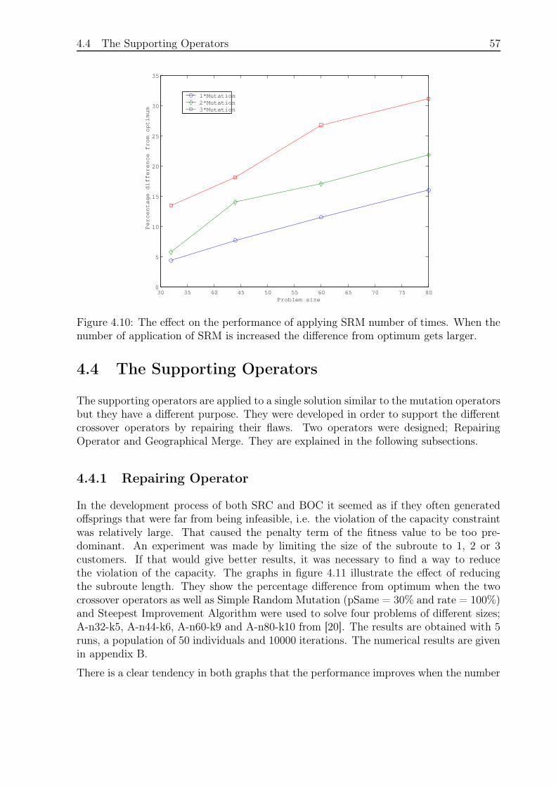
4.4 The Supporting Operators 57
30 35 40 45 50 55 60 65 70 75 800
5
10
15
20
25
30
35
Percentage difference from optimum
Problem size
1*Mutation2*Mutation3*Mutation
Figure 4.10: The effect on the performance of applying SRM number of times. When thenumber of application of SRM is increased the difference from optimum gets larger.
4.4 The Supporting Operators
The supporting operators are applied to a single solution similar to the mutation operatorsbut they have a different purpose. They were developed in order to support the differentcrossover operators by repairing their flaws. Two operators were designed; RepairingOperator and Geographical Merge. They are explained in the following subsections.
4.4.1 Repairing Operator
In the development process of both SRC and BOC it seemed as if they often generatedoffsprings that were far from being infeasible, i.e. the violation of the capacity constraintwas relatively large. That caused the penalty term of the fitness value to be too pre-dominant. An experiment was made by limiting the size of the subroute to 1, 2 or 3customers. If that would give better results, it was necessary to find a way to reducethe violation of the capacity. The graphs in figure 4.11 illustrate the effect of reducingthe subroute length. They show the percentage difference from optimum when the twocrossover operators as well as Simple Random Mutation (pSame = 30% and rate = 100%)and Steepest Improvement Algorithm were used to solve four problems of different sizes;A-n32-k5, A-n44-k6, A-n60-k9 and A-n80-k10 from [20]. The results are obtained with 5runs, a population of 50 individuals and 10000 iterations. The numerical results are givenin appendix B.
There is a clear tendency in both graphs that the performance improves when the number
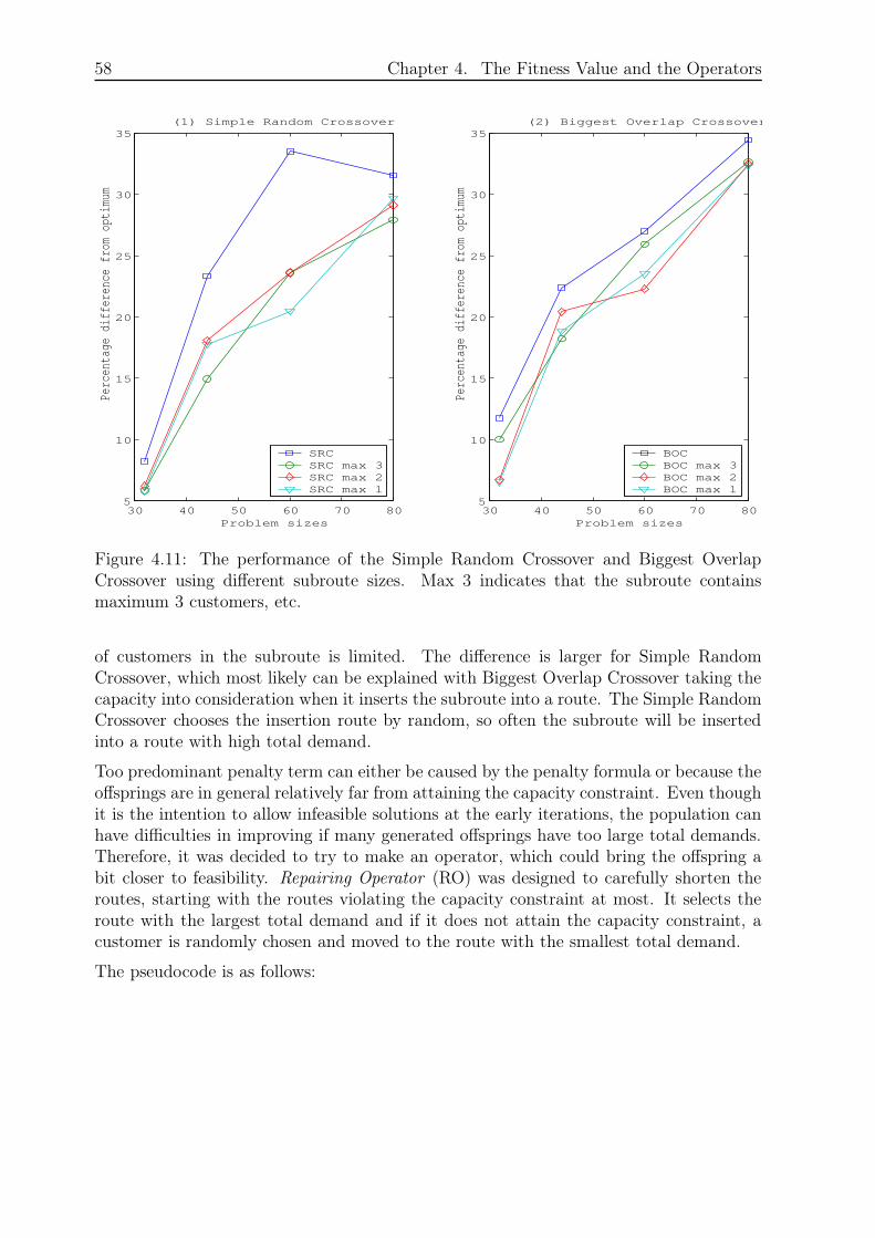
58 Chapter 4. The Fitness Value and the Operators
30 40 50 60 70 805
10
15
20
25
30
35(1) Simple Random Crossover
Problem sizes
Perc
enta
ge d
iffe
renc
e fr
om o
ptim
um
SRCSRC max 3SRC max 2SRC max 1
30 40 50 60 70 805
10
15
20
25
30
35(2) Biggest Overlap Crossover
Problem sizes
Perc
enta
ge d
iffe
renc
e fr
om o
ptim
umBOCBOC max 3BOC max 2BOC max 1
Figure 4.11: The performance of the Simple Random Crossover and Biggest OverlapCrossover using different subroute sizes. Max 3 indicates that the subroute containsmaximum 3 customers, etc.
of customers in the subroute is limited. The difference is larger for Simple RandomCrossover, which most likely can be explained with Biggest Overlap Crossover taking thecapacity into consideration when it inserts the subroute into a route. The Simple RandomCrossover chooses the insertion route by random, so often the subroute will be insertedinto a route with high total demand.
Too predominant penalty term can either be caused by the penalty formula or because theoffsprings are in general relatively far from attaining the capacity constraint. Even thoughit is the intention to allow infeasible solutions at the early iterations, the population canhave difficulties in improving if many generated offsprings have too large total demands.Therefore, it was decided to try to make an operator, which could bring the offspring abit closer to feasibility. Repairing Operator (RO) was designed to carefully shorten theroutes, starting with the routes violating the capacity constraint at most. It selects theroute with the largest total demand and if it does not attain the capacity constraint, acustomer is randomly chosen and moved to the route with the smallest total demand.
The pseudocode is as follows:
4.4 The Supporting Operators 59
Repair(offspring)
jMax ← the index of the route in the offspring with largest total demandmaxDem ← the total demand of route jMaxjMin ← the index of the route in the offspring with smallest total demand
if maxDem > Krandomly choose a customer from route jMaxdelete the customer from route jMininsert the customer at the end of route jMin
return offspring
4.4.2 Geographical Merge
The role of Geographical Merge (GM) is to merge two routes, which are close to each other,within the same individual. Horizontal Line Crossover and Uniform Crossover, explainedin section 4.2.3 and 4.2.4 respectively, tend to generate offsprings with relatively shortroutes. In order to illustrate that, the average difference from the capacity was calculated,separately for the routes with too much total demand and for those with total demandwithin the capacity of the vehicles. Equation 4.8 illustrates the formula, which was usedto calculate the difference dp for routes attaining the capacity constraint, where p standsfor plus. If a route does no contain any routes of either kind the difference is set tozero. The formula for the routes violating the capacity constraint is corresponding. Thefollowing formula shows the difference for the routes attaining the capacity constraint.
dp =
∑
(K − totdemp)
nrp,r
(4.8)
where:
K is the capacity of the vehicles,totdemp is the total demand of a route r where it is less than K andnrp denotes number of routes with total demand less than K.
In the following figures the results, which were obtained by solving problem instance A-n80-k10 from [20] using the two crossover operators, Simple Random Mutation (pSame= 30% and rate = 100%) and Steepest Improvement Algorithm. The algorithm was runonce with a population size 50 and 10000 iterations. The capacity of the vehicles is 100.
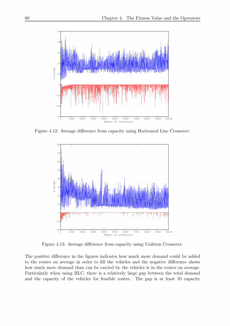
60 Chapter 4. The Fitness Value and the Operators
0 1000 2000 3000 4000 5000 6000 7000 8000 9000 10000−30
−20
−10
0
10
20
30
40
50
Number of iterations
K−totdem
Figure 4.12: Average difference from capacity using Horizontal Line Crossover.
0 1000 2000 3000 4000 5000 6000 7000 8000 9000 10000−20
−10
0
10
20
30
40
50
60
70
80
Number of iterations
K−totdem
Figure 4.13: Average difference from capacity using Uniform Crossover.
The positive difference in the figures indicates how much more demand could be addedto the routes on average in order to fill the vehicles and the negative difference showshow much more demand than can be carried by the vehicles is in the routes on average.Particularly when using HLC, there is a relatively large gap between the total demandand the capacity of the vehicles for feasible routes. The gap is at least 10 capacity
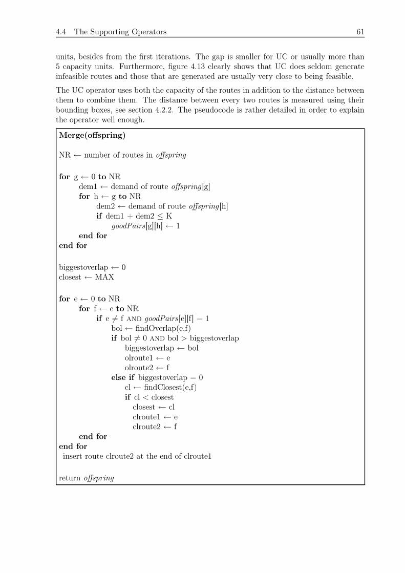
4.4 The Supporting Operators 61
units, besides from the first iterations. The gap is smaller for UC or usually more than5 capacity units. Furthermore, figure 4.13 clearly shows that UC does seldom generateinfeasible routes and those that are generated are usually very close to being feasible.
The UC operator uses both the capacity of the routes in addition to the distance betweenthem to combine them. The distance between every two routes is measured using theirbounding boxes, see section 4.2.2. The pseudocode is rather detailed in order to explainthe operator well enough.
Merge(offspring)
NR ← number of routes in offspring
for g ← 0 to NRdem1 ← demand of route offspring [g]for h ← g to NR
dem2 ← demand of route offspring [h]if dem1 + dem2 ≤ K
goodPairs[g][h] ← 1end for
end for
biggestoverlap ← 0closest ← MAX
for e ← 0 to NRfor f ← e to NR
if e 6= f and goodPairs[e][f] = 1bol ← findOverlap(e,f)if bol 6= 0 and bol > biggestoverlap
biggestoverlap ← bololroute1 ← eolroute2 ← f
else if biggestoverlap = 0cl ← findClosest(e,f)if cl < closest
closest ← clclroute1 ← eclroute2 ← f
end forend forinsert route clroute2 at the end of clroute1
return offspring
62 Chapter 4. The Fitness Value and the Operators
The operator is applied on a single individual. It starts by identifying pairs of routesthat together have the total demand within the limits of the capacity, thus it does notgenerate infeasible routes. Then the pair of routes closest to each other is selected. Ifthe bounding boxes of the routes overlap, the pair with the largest overlap is chosen.Otherwise, it selects the pair with the shortest distance between the bounding boxes.Finally, the routes are merged together by adding the one route at the end of the other.
4.5 Summary
In this chapter the development process of the fitness value and 7 operators is dis-cussed. Four crossover operators are explained; Simple Random Crossover, Biggest Over-lap Crossover, Horizontal Line Crossover and Uniform Crossover. Simple Random Muta-tion, the only mutation operator, is described and also two supporting operators; Repair-ing Operator and Geographical Merge. In the next chapter some implementation issuesare discussed.
63
Chapter 5
Implementation
In this chapter implementation issues are discussed, such as information about the com-puter, the experiments that were carried out and computation of Euclidean distances,among other things.
Computational experiments were carried out on a Zitech PC with a 800 MHz AMDAthlon(tm) processor. The program was implemented using the Java 1.3.1_01 StandardEdition and compiled using the java compiler.
The CPU-time was calculated using the function currentTimeMillis() in Java. It returnsthe current time in milliseconds since midnight January 1, 1970 GMT. The function isused right before the algorithm is applied in the code and again afterwards. The executiontime of the algorithm is the difference between two measurements.
The cost of travelling between every two customers was calculated using Euclidean dis-tances. Some problem instances have been calculated using real numbers in which thebest results are presented. Others are calculated with integers. When integers are used,the rounding function Nearest Integer function nint was used to convert the Euclideandistances into integers. The function returns the integer closest to the given numberand half-integers are rounded up to the smallest integer bigger than the number, i.e.nint(1.4) = 1, nint(3.8) = 4 and nint(5.5) = 6. When Java rounds real numbers, allnumbers are rounded down to the nearest integer. Therefore, a constant 0.5 was addedto all the real numbers in order to simulate nint. For instance, Java rounds 3.8 down to3 by Java but by adding 0.5 to it, 3.8 + 0.5 = 4.3, it is instead rounded ”up” to 4!
In section 2.2.2 the representation of the VRP solution used in this project is described.The population is implemented as a 3-dimensional array M × dim × dim, where M is thepopulation size and dim is the number of customers in each problem. So Pop[2][5][3] = 5means that customer no. 5 is visited number 4 in route 6 in the third individual in thepopulation (indices start in 0 in Java).
The advantage of presenting the population in this way is that it is very simple to imple-ment. Furthermore, it simplifies communication and gives a good overview. The drawbackis that it contains a lot of empty spaces that use memory, where either the number ofcustomers is less than dim or the number of routes is less than dim. The memory need

64 Chapter 5. Implementation
of the population could be reduced by using upper bound on the number of customerswithin a route or on the number of routes, based on the problem to be solved. However,one should be careful about using upper bounds because Java is not able to enlarge anarray dynamically. Thus if the program tries to insert a customer outside the array theprogram terminates.
In order to save computational time, the total cost of each individual was kept in separatearrays for the cost and the penalty. Since the program used a steady-state algorithm (seesection 2.2.2) only few solutions were changed in each iteration. When a solution waschanged, it was noted in the cost and the penalty array and next time it was selected thecost was recalculated. In a similar way the bounding boxes were also kept in an array.
65
Chapter 6
Parameter Tuning
Many parameters are involved in solving VRP with GA. The values of those need tobe tuned. Good parameter tuning is important for all GA to generate good solutions.Usually, it is complex to tune the parameters because the relationship between them canbe rather complicated and unclear. Most algorithms contain many parameters and themore they get the more time consuming the tuning becomes. Ideally, all parametersshould be tuned but that is in general too time consuming. However, it is important totune as many as possible. In the following section all parameters are listed, it is explainedhow they were tuned and the values they were given are shown.
6.1 The Parameters and the Tuning Description
The parameters are divided into two groups of more or less important parameters. In thegroup of more important parameters are those that are believed to have more influence onthe effectivity of the algorithm. In the other group are parameters of less significance andthe effect of some of them has been discussed in the previous chapter. The parametersare listed in the two tables below:
1. The Population size (M).2. The rate of SRM.3. The rate of RO.4. The rate of GM.
Table 6.1: The more important parameters.
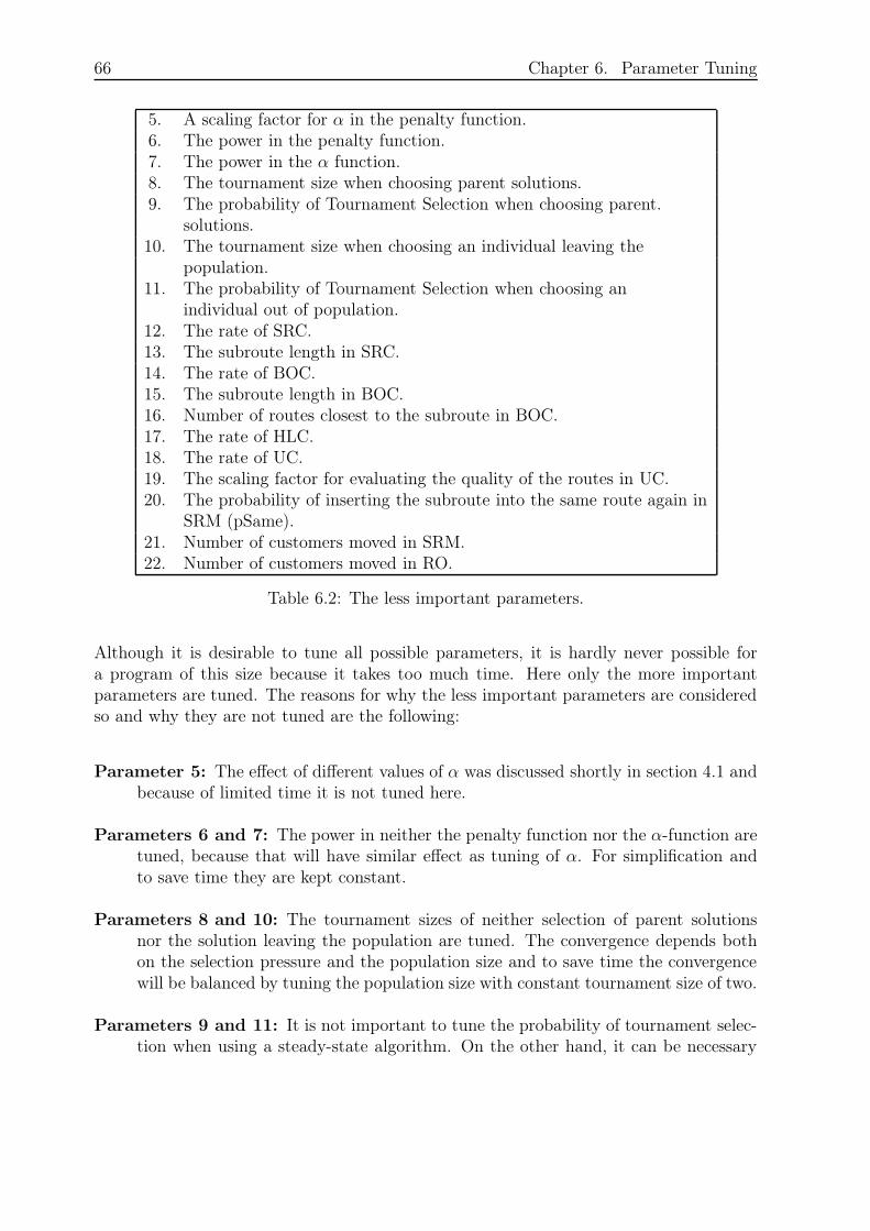
66 Chapter 6. Parameter Tuning
5. A scaling factor for α in the penalty function.6. The power in the penalty function.7. The power in the α function.8. The tournament size when choosing parent solutions.9. The probability of Tournament Selection when choosing parent.
solutions.10. The tournament size when choosing an individual leaving the
population.11. The probability of Tournament Selection when choosing an
individual out of population.12. The rate of SRC.13. The subroute length in SRC.14. The rate of BOC.15. The subroute length in BOC.16. Number of routes closest to the subroute in BOC.17. The rate of HLC.18. The rate of UC.19. The scaling factor for evaluating the quality of the routes in UC.20. The probability of inserting the subroute into the same route again in
SRM (pSame).21. Number of customers moved in SRM.22. Number of customers moved in RO.
Table 6.2: The less important parameters.
Although it is desirable to tune all possible parameters, it is hardly never possible fora program of this size because it takes too much time. Here only the more importantparameters are tuned. The reasons for why the less important parameters are consideredso and why they are not tuned are the following:
Parameter 5: The effect of different values of α was discussed shortly in section 4.1 andbecause of limited time it is not tuned here.
Parameters 6 and 7: The power in neither the penalty function nor the α-function aretuned, because that will have similar effect as tuning of α. For simplification andto save time they are kept constant.
Parameters 8 and 10: The tournament sizes of neither selection of parent solutionsnor the solution leaving the population are tuned. The convergence depends bothon the selection pressure and the population size and to save time the convergencewill be balanced by tuning the population size with constant tournament size of two.
Parameters 9 and 11: It is not important to tune the probability of tournament selec-tion when using a steady-state algorithm. On the other hand, it can be necessary
6.1 The Parameters and the Tuning Description 67
to reduce the selection pressure by applying the tournament selection with a certainprobability when generational algorithms are used, see page 20.
Parameters 12, 14, 17 and 18: The probability of applying a crossover operator is nottuned. Skipping a crossover in some iterations can be done to be better able to pre-serve a part of the population from one iteration to another. That is not importanthere because a steady-state algorithm is used.
Parameters 13 and 15: The lengths of the subroutes in SRC and BOC are not tunedbecause it is important to keep some randomness in the crossover operators.
Parameters 16, 19 and 20: The number of routes or candidates in BOC, is not tunedsince it will most likely not have much influence compared to the time it takes totune it. For the same reasons a possible scaling factor in UC and pSame are nottuned. The parameter pSame is set to 30%, which has worked out fine during thedevelopment process of the project.
Parameters 21 and 22: Instead of tuning the number of customers moved in SRM andRO directly they are tuned at some degree by tuning the rate of the operators whereit is possible to apply them twice.
Two algorithms are defined; a fast algorithm with 10000 iterations and a slow algorithmwith 100000 iterations. The algorithms are tuned for different sets of population sizesbut parameters 2, 3 and 4 are tuned for the same values for both algorithms. Since thereis not a linear correlation between the population size and the number of iterations, theslow algorithm is not necessarily expected to perform better than the fast algorithm.
The problem instances that are used for both tuning and testing are divided into twogroups of small instances with less than 100 customers and large instances with 100 cus-tomers or more. The size of the large instances limits the possible population size to 100due to the memory of the computer that is used. Furthermore, running the slow algo-rithm using a relatively large population for large problems is extremely time consuming.Thus, the large instances are only tuned for the fast algorithm and smaller populations.The values of parameters 2, 3 and 4 for the slow algorithm and the large instances areborrowed from the tuning of the small instances for the slow algorithms. The possiblevalues of parameters are chosen based on the experience that has been gained during thedevelopment process. The following tables show the possible values for small problemsusing fast and slow algorithm and large problems using fast algorithm.
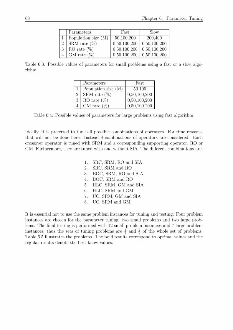
68 Chapter 6. Parameter Tuning
Parameters Fast Slow1 Population size (M) 50,100,200 200,4002 SRM rate (%) 0,50,100,200 0,50,100,2003 RO rate (%) 0,50,100,200 0,50,100,2004 GM rate (%) 0,50,100,200 0,50,100,200
Table 6.3: Possible values of parameters for small problems using a fast or a slow algo-rithm.
Parameters Fast1 Population size (M) 50,1002 SRM rate (%) 0,50,100,2003 RO rate (%) 0,50,100,2004 GM rate (%) 0,50,100,200
Table 6.4: Possible values of parameters for large problems using fast algorithm.
Ideally, it is preferred to tune all possible combinations of operators. For time reasons,that will not be done here. Instead 8 combinations of operators are considered. Eachcrossover operator is tuned with SRM and a corresponding supporting operator, RO orGM. Furthermore, they are tuned with and without SIA. The different combinations are:
1. SRC, SRM, RO and SIA2. SRC, SRM and RO3. BOC, SRM, RO and SIA4. BOC, SRM and RO5. HLC, SRM, GM and SIA6. HLC, SRM and GM7. UC, SRM, GM and SIA8. UC, SRM and GM
It is essential not to use the same problem instances for tuning and testing. Four probleminstances are chosen for the parameter tuning; two small problems and two large prob-lems. The final testing is performed with 12 small problem instances and 7 large probleminstances, thus the sets of tuning problems are 1
7and 2
9of the whole set of problems.
Table 6.5 illustrates the problems. The bold results correspond to optimal values and theregular results denote the best know values.
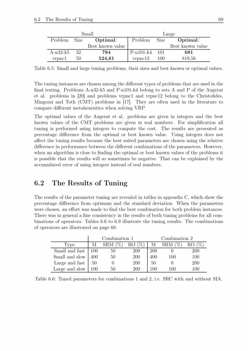
6.2 The Results of Tuning 69
Small LargeProblem Size Optimal/ Problem Size Optimal/
Best known value Best known valueA-n32-k5 32 784 P-n101-k4 101 681vrpnc1 50 524,61 vrpnc12 100 819,56
Table 6.5: Small and large tuning problems, their sizes and best known or optimal values.
The tuning instances are chosen among the different types of problems that are used in thefinal testing. Problems A-n32-k5 and P-n101-k4 belong to sets A and P of the Augeratet al. problems in [20] and problems vrpnc1 and vrpnc12 belong to the Christofides,Mingozzi and Toth (CMT) problems in [17]. They are often used in the literature tocompare different metaheuristics when solving VRP.
The optimal values of the Augerat et al. problems are given in integers and the bestknown values of the CMT problems are given in real numbers. For simplification alltuning is performed using integers to compute the cost. The results are presented aspercentage difference from the optimal or best known value. Using integers does notaffect the tuning results because the best suited parameters are chosen using the relativedifference in performance between the different combinations of the parameters. However,when an algorithm is close to finding the optimal or best known values of the problems itis possible that the results will so sometimes be negative. That can be explained by theaccumulated error of using integers instead of real numbers.
6.2 The Results of Tuning
The results of the parameter tuning are revealed in tables in appendix C, which show thepercentage difference from optimum and the standard deviation. When the parameterswere chosen, an effort was made to find the best combination for both problem instances.There was in general a fine consistency in the results of both tuning problems for all com-binations of operators. Tables 6.6 to 6.9 illustrate the tuning results. The combinationsof operators are illustrated on page 68.
Combination 1 Combination 2Type M SRM (%) RO (%) M SRM (%) RO (%)
Small and fast 100 50 200 200 0 200Small and slow 400 50 200 400 100 100Large and fast 50 0 200 50 0 200Large and slow 100 50 200 100 100 100
Table 6.6: Tuned parameters for combinations 1 and 2, i.e. SRC with and without SIA.
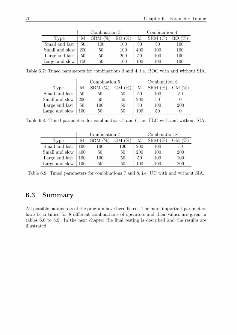
70 Chapter 6. Parameter Tuning
Combination 3 Combination 4Type M SRM (%) RO (%) M SRM (%) RO (%)
Small and fast 50 100 100 50 50 100Small and slow 200 50 100 400 100 100Large and fast 50 50 200 50 100 100Large and slow 100 50 100 100 100 100
Table 6.7: Tuned parameters for combinations 3 and 4, i.e. BOC with and without SIA.
Combination 5 Combination 6Type M SRM (%) GM (%) M SRM (%) GM (%)
Small and fast 50 50 50 50 100 50Small and slow 200 50 50 200 50 0Large and fast 50 100 50 50 100 200Large and slow 100 50 50 100 50 0
Table 6.8: Tuned parameters for combinations 5 and 6, i.e. HLC with and without SIA.
Combination 7 Combination 8Type M SRM (%) GM (%) M SRM (%) GM (%)
Small and fast 100 100 100 200 100 50Small and slow 400 50 50 200 100 200Large and fast 100 100 50 50 100 100Large and slow 100 50 50 100 100 200
Table 6.9: Tuned parameters for combinations 7 and 8, i.e. UC with and without SIA.
6.3 Summary
All possible parameters of the program have been listed. The more important parametershave been tuned for 8 different combinations of operators and their values are given intables 6.6 to 6.9. In the next chapter the final testing is described and the results areillustrated.
71
Chapter 7
Testing
In this chapter the testing of the operators is described and the results are illustrated. Theoperators are tested by the the means of 8 different combinations that are illustrated onpage 68 and the testing is performed using the parameters found in tables 6.6 to 6.9 in theprevious chapter. The tests are made in two steps. Firstly, all combinations of operatorsare tested in order to choose the best combination. Secondly, the best combination isapplied to an additional number of problems and the results are compared to recentlyproposed results of other metaheuristics.
7.1 The Benchmark Problems
The testing is performed on 12 small and 7 large problems, which are listed in the tablesbelow. It would have been desirable to perform the testing using more large problemsbut large problems with known optimal or best values were difficult to find. The optimalvalues are illustrated bold.
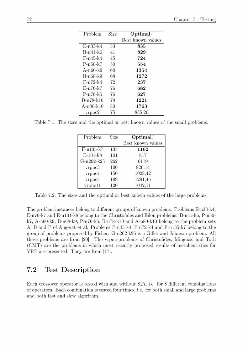
72 Chapter 7. Testing
Problem Size Optimal/Best known values
E-n33-k4 33 835B-n41-k6 41 829F-n45-k4 45 724P-n50-k7 50 554A-n60-k9 60 1354B-n68-k9 68 1272F-n72-k4 72 237E-n76-k7 76 682P-n76-k5 76 627B-n78-k10 78 1221A-n80-k10 80 1763
vrpnc2 75 835,26
Table 7.1: The sizes and the optimal or best known values of the small problems.
Problem Size Optimal/Best known values
F-n135-k7 135 1162E-101-k8 101 817
G-n262-k25 262 6119vrpnc3 100 826,14vrpnc4 150 1028,42vrpnc5 199 1291,45vrpnc11 120 1042,11
Table 7.2: The sizes and the optimal or best known values of the large problems.
The problem instances belong to different groups of known problems. Problems E-n33-k4,E-n76-k7 and E-n101-k8 belong to the Christofides and Eilon problems. B-n41-k6, P-n50-k7, A-n60-k9, B-n68-k9, P-n76-k5, B-n78-k10 and A-n80-k10 belong to the problem setsA, B and P of Augerat et al. Problems F-n45-k4, F-n72-k4 and F-n135-k7 belong to thegroup of problems proposed by Fisher. G-n262-k25 is a Gillet and Johnson problem. Allthese problems are from [20]. The vrpnc-problems of Christofides, Mingozzi and Toth(CMT) are the problems in which most recently proposed results of metaheuristics forVRP are presented. They are from [17].
7.2 Test Description
Each crossover operator is tested with and without SIA, i.e. for 8 different combinationsof operators. Each combination is tested four times, i.e. for both small and large problemsand both fast and slow algorithm.
7.3 The Results 73
The first part of the testing is performed in order to choose the best possible combinationfor each problem size and each type of algorithm. Three small and three large probleminstances are selected from tables ?? and 7.2: B-n41-k6, B-n68-k9 and vrpnc2 for smallproblems and vrpnc3, vrpnc9 and vrpnc11 for large problems. The different combinationsare applied to these problems and the best one is selected, primarily considering theaccuracy. That is measured by the difference from the optimum or the best known valueof each problem. The selection is based on the average performance of 10 runs. Boxplotshelp with illustrating the difference in performance between the operators. Consider theresults in a vector vc where c is the index of the considered combination. A boxplot drawsthe median of vc, the minimum and the maximum value, the 1st and the 3rd quartile.
In the second part of the testing, the best combination is applied to the rest of theproblems within each size for each type of algorithm. For each size the results of the fastand the slow algorithm are compared. The more accurate algorithm is chosen. The resultsare presented for solving the small CMT problems with the best algorithm for the smallproblems and the large CMT problems with the best algorithm for the large problems. Theresults are compared to the proposed results of three Tabu Search heuristics; Taburoute,Taillard’s Algorithm and Adaptive memory [4], and the Hybrid Genetic Algorithm 2.1.4.
7.3 The Results
In the following 7 subsections the results are presented. The first three subsections involvethe testing for the small problems. The next three sections illustrate the results for thelarge problems. In the final subsection, the results of the comparison with proposed theTabu Search heuristics and the Hybrid Genetic Algorithm are stated.
7.3.1 Small Problems and Fast Algorithm
In order to choose the best combination of operators, the combinations are comparedusing the fast algorithm to solve the small problems. The results of solving the threesmall problem instances are illustrated in the following four tables. Each table illustratesthe results of using one of the crossover operators with or without SIA. The results arepresented as the average percentage difference from optimum or best know value, standarddeviation and time. The combinations are explained on page 68 and the parameters areshown in tables 6.6 to 6.9.
74 Chapter 7. Testing
Combination 1 Combination 2
Problem Diff. from Std. dev. Time Diff. from Std. dev. Timeopt./best (%) σ (ms) opt./best (%) σ (ms)
B-n41-k6 5,1 3,44 5120 7,55 4,31 2273B-n68-k9 14,11 3,8 10297 23,23 5,83 5094vrpnc2 16,21 2,33 10453 30,96 6,48 6305
Average 11,81 3,19 8623 20,58 5,54 4557
Table 7.3: Results of solving the small problems with the fast algorithm using SRC withand without SIA.
Combination 3 Combination 4
Problem Diff. from Std. dev. Time Diff. from Std. dev. Timeopt./best (%) σ (ms) opt./best (%) σ (ms)
B-n41-k6 8,6 4,81 4291 14,68 4,44 1999B-n68-k9 20,74 3,66 9371 39,16 6,46 4666vrpnc2 14,13 2,67 13220 32,4 3,59 5894
Average 14,49 3,71 8961 28,75 4,83 4186
Table 7.4: Results of solving the small problems with the fast algorithm using BOC withand without SIA.
Combination 5 Combination 6
Problem Diff. from Std. dev. Time Diff. from Std. dev. Timeopt./best (%) σ (ms) opt./best (%) σ (ms)
B-n41-k6 12,34 4,99 2768 16,61 6,35 2545B-n68-k9 11,47 2,47 5885 20,47 4,11 5771vrpnc2 25,41 4,4 9111 49,03 5,8 7206
Average 16,41 3,95 5921 28,70 5,42 5174
Table 7.5: Results of solving the small problems with the fast algorithm using HLC withand without SIA.
Combination 7 Combination 8
Problem Diff. from Std. dev. Time Diff. from Std. dev. Timeopt./best (%) σ (ms) opt./best (%) σ (ms)
B-n41-k6 8,06 4,23 5008 15,96 4,14 2685B-n68-k9 12,51 4,25 11027 19,69 3,69 6084vrpnc2 13,26 1,96 17548 23,49 2,15 7286
Average 11,28 3,48 11194 19,71 3,32 5342
Table 7.6: Results of solving the small problems with the fast algorithm using UC withand without SIA.
The boxplot below illustrates the results graphically. Note that the performance of eachcombination is presented as average in the tables and as the median in the boxplot. Alsonote that combinations 1, 3, 5 and 7 are with SIA and 2, 4, 6 and 8 are without SIA.
7.3 The Results 75
1 2 3 4 5 6 7 8
5
10
15
20
25
30
35
40
45
50
Percentage difference from optimum
Combinations
Figure 7.1: The performance of the different combinations for the fast algorithm and thesmall problems. Combination 7 gives the best results.
The results illustrate that combination 7 with UC and SIA performs best. Althoughcombination 1 with SRC and SIA provides almost as good results on average. It is quiteclear that SIA has rather great improving effect for all the crossover operators but it takestime. For instance, SIA reduces the difference from optimum by almost half for BOC, seetable 7.4. BOC and HLC do not perform well enough. Combination 7 is the most timeconsuming one combination and combination 5 is the least time consuming of those thatare supplied with SIA.
Combination 7 is now applied to the rest of the small problems using the fast algorithmand the results of all problems are illustrated in the table 7.7. The results of B-n41-k6,B-n68-k9 and vrpnc2 are obtained from table 7.6

76 Chapter 7. Testing
Problem Diff. from Std. dev. Timeopt. (%) σ (ms)
E-n33-k4 4,14 1,99 2857B-n41-k6 8,06 4,23 5008F-n45-k4 4,91 2,59 753P-n50-k7 7,27 3,64 4601B-n56-k7 7,42 2,38 6019A-n60-k9 12,82 1,38 6078B-n68-k9 12,51 4,25 11027F-n72-k4 25,3 7,62 14101P-n76-k5 10,25 2,58 12075B-n78-k10 13,58 1,91 10260A-n80-k10 16,91 3,5 10836
vrpnc2 13,26 1,96 17548
Average 11,37 3,17 8430
Table 7.7: Results of solving all the small problems with the fast algorithm using combi-nation 7, i.e. UC and SIA.
7.3.2 Small Problems and Slow Algorithm
In this subsection the combinations of operators are compared for solving the small prob-lems with the slow algorithm. The results are shown in the tables 7.8 to 7.11. Each tableincludes the results of each crossover operator with or without SIA. Different combina-tions are explained on page 68 and the tuned parameters are shown in tables 6.6 and6.9.
Combination 1 Combination 2
Problem Diff. from Std. dev. Time Diff. from Std. dev. Timeopt./best (%) σ (ms) opt./best (%) σ (ms)
B-n41-k6 2,41 1,73 46842 4,91 2 20774B-n68-k9 4,03 1,8 100492 14,25 5,56 46985vrpnc2 6,08 0,94 96782 18,41 1,66 59957
Average 4,17 1,49 81372 12,52 3,07 42572
Table 7.8: Results of solving the small problems with the slow algorithm using SRC andSIA.
7.3 The Results 77
Combination 3 Combination 4
Problem Diff. from Std. dev. Time Diff. from Std. dev. Timeopt./best (%) σ (ms) opt./best (%) σ (ms)
B-n41-k6 5,05 3,31 42002 6,12 3,56 19865B-n68-k9 5,86 3,4 93619 19,51 6,11 45559vrpnc2 5,28 2,09 142070 18,57 2,95 55418
Average 5,40 2,93 92564 14,73 4,21 40281
Table 7.9: Results of solving the small problems with the slow algorithm using BOC withand without SIA.
Combination 5 Combination 6
Problem Diff. from Std. dev. Time Diff. from Std. dev. Timeopt./best (%) σ (ms) opt./best (%) σ (ms)
B-n41-k6 5,17 2,05 42782 10,75 3,87 20593B-n68-k9 9,24 0,99 83666 12,54 2,18 44186vrpnc2 31,81 3,74 68152 26,58 3,24 59867
Average 15,41 2,26 64867 16,62 3,10 41549
Table 7.10: Results of solving the small problems with the slow algorithm using HLCwith and without SIA.
Combination 7 Combination 8
Problem Diff. from Std. dev. Time Diff. from Std. dev. Timeopt./best (%) σ (ms) opt./best (%) σ (ms)
B-n41-k6 0,83 0,57 54246 3,63 2,83 37645B-n68-k9 6,58 2,27 101244 10,53 1,89 85522vrpnc2 7,2 2,07 165125 11,99 2,4 113309
Average 4,87 1,64 106872 8,72 2,37 78825
Table 7.11: Results of solving the small problems with the slow algorithm using UC withand without SIA.
The results are also illustrated in the boxplot below. Note that the performance of eachcombination is presented as average in the tables and as the median in the boxplot. Alsonote that combinations 1, 3, 5 and 7 are with SIA and 2, 4, 6 and 8 are without SIA.
78 Chapter 7. Testing
1 2 3 4 5 6 7 8
0
5
10
15
20
25
30
Percentage difference from optimum
Combinations
Figure 7.2: The performance of the different combinations for the slow algorithm andthe small problems. Combination 1 gives the best results, but combinations 3 and 7 alsoperform quite well.
Combination 1 with SRC and SIA is the best combination. However, combinations 3with BOC and SIA and 7 with UC and SIA do also perform well. As for the fast algorithm,application of SIA improves the results of the crossover operators considerably. On theother hand, combinations with SIA are more time consuming. Both combinations withHLC perform particularly bad compared to the other combinations.
In table 7.12 the results of applying combination 1 using the slow algorithm to solve thesmall problems are shown. The results of problems B-n41-k6, B-n68-k9 and vrpnc2 arefrom table 7.8.
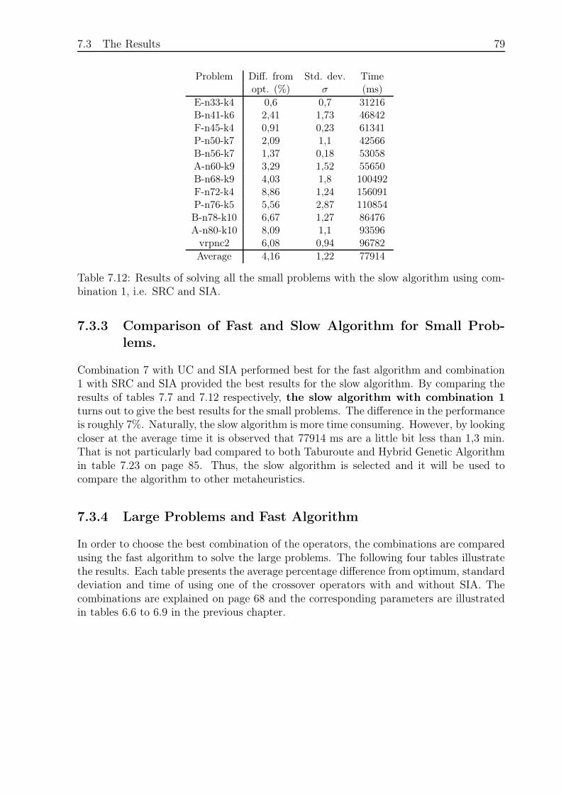
7.3 The Results 79
Problem Diff. from Std. dev. Timeopt. (%) σ (ms)
E-n33-k4 0,6 0,7 31216B-n41-k6 2,41 1,73 46842F-n45-k4 0,91 0,23 61341P-n50-k7 2,09 1,1 42566B-n56-k7 1,37 0,18 53058A-n60-k9 3,29 1,52 55650B-n68-k9 4,03 1,8 100492F-n72-k4 8,86 1,24 156091P-n76-k5 5,56 2,87 110854B-n78-k10 6,67 1,27 86476A-n80-k10 8,09 1,1 93596
vrpnc2 6,08 0,94 96782
Average 4,16 1,22 77914
Table 7.12: Results of solving all the small problems with the slow algorithm using com-bination 1, i.e. SRC and SIA.
7.3.3 Comparison of Fast and Slow Algorithm for Small Prob-
lems.
Combination 7 with UC and SIA performed best for the fast algorithm and combination1 with SRC and SIA provided the best results for the slow algorithm. By comparing theresults of tables 7.7 and 7.12 respectively, the slow algorithm with combination 1turns out to give the best results for the small problems. The difference in the performanceis roughly 7%. Naturally, the slow algorithm is more time consuming. However, by lookingcloser at the average time it is observed that 77914 ms are a little bit less than 1,3 min.That is not particularly bad compared to both Taburoute and Hybrid Genetic Algorithmin table 7.23 on page 85. Thus, the slow algorithm is selected and it will be used tocompare the algorithm to other metaheuristics.
7.3.4 Large Problems and Fast Algorithm
In order to choose the best combination of the operators, the combinations are comparedusing the fast algorithm to solve the large problems. The following four tables illustratethe results. Each table presents the average percentage difference from optimum, standarddeviation and time of using one of the crossover operators with and without SIA. Thecombinations are explained on page 68 and the corresponding parameters are illustratedin tables 6.6 to 6.9 in the previous chapter.
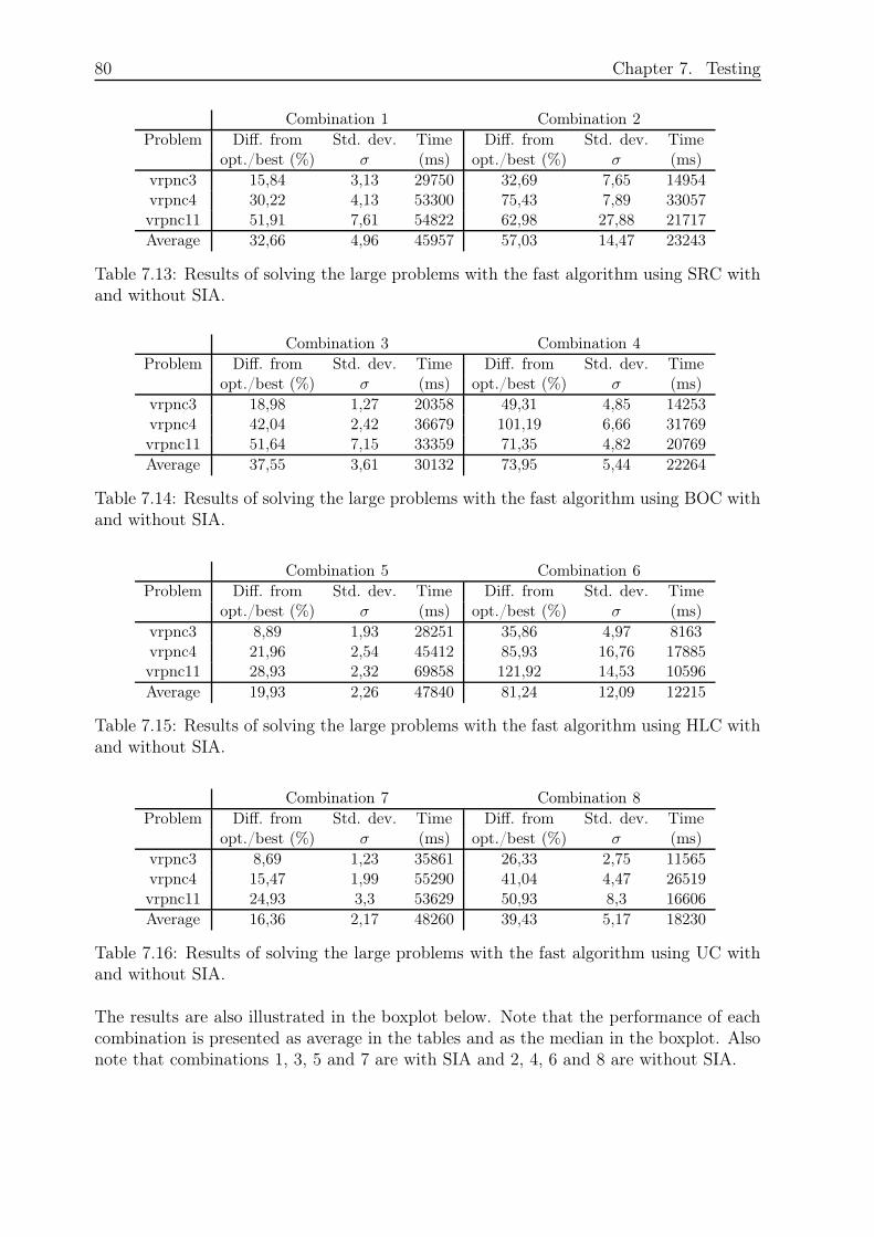
80 Chapter 7. Testing
Combination 1 Combination 2
Problem Diff. from Std. dev. Time Diff. from Std. dev. Timeopt./best (%) σ (ms) opt./best (%) σ (ms)
vrpnc3 15,84 3,13 29750 32,69 7,65 14954vrpnc4 30,22 4,13 53300 75,43 7,89 33057vrpnc11 51,91 7,61 54822 62,98 27,88 21717
Average 32,66 4,96 45957 57,03 14,47 23243
Table 7.13: Results of solving the large problems with the fast algorithm using SRC withand without SIA.
Combination 3 Combination 4
Problem Diff. from Std. dev. Time Diff. from Std. dev. Timeopt./best (%) σ (ms) opt./best (%) σ (ms)
vrpnc3 18,98 1,27 20358 49,31 4,85 14253vrpnc4 42,04 2,42 36679 101,19 6,66 31769vrpnc11 51,64 7,15 33359 71,35 4,82 20769
Average 37,55 3,61 30132 73,95 5,44 22264
Table 7.14: Results of solving the large problems with the fast algorithm using BOC withand without SIA.
Combination 5 Combination 6
Problem Diff. from Std. dev. Time Diff. from Std. dev. Timeopt./best (%) σ (ms) opt./best (%) σ (ms)
vrpnc3 8,89 1,93 28251 35,86 4,97 8163vrpnc4 21,96 2,54 45412 85,93 16,76 17885vrpnc11 28,93 2,32 69858 121,92 14,53 10596
Average 19,93 2,26 47840 81,24 12,09 12215
Table 7.15: Results of solving the large problems with the fast algorithm using HLC withand without SIA.
Combination 7 Combination 8
Problem Diff. from Std. dev. Time Diff. from Std. dev. Timeopt./best (%) σ (ms) opt./best (%) σ (ms)
vrpnc3 8,69 1,23 35861 26,33 2,75 11565vrpnc4 15,47 1,99 55290 41,04 4,47 26519vrpnc11 24,93 3,3 53629 50,93 8,3 16606
Average 16,36 2,17 48260 39,43 5,17 18230
Table 7.16: Results of solving the large problems with the fast algorithm using UC withand without SIA.
The results are also illustrated in the boxplot below. Note that the performance of eachcombination is presented as average in the tables and as the median in the boxplot. Alsonote that combinations 1, 3, 5 and 7 are with SIA and 2, 4, 6 and 8 are without SIA.
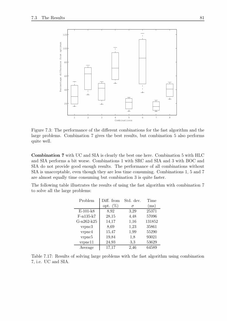
7.3 The Results 81
1 2 3 4 5 6 7 8
20
40
60
80
100
120
Percentage difference from optimum
Combinations
Figure 7.3: The performance of the different combinations for the fast algorithm and thelarge problems. Combination 7 gives the best results, but combination 5 also performsquite well.
Combination 7 with UC and SIA is clearly the best one here. Combination 5 with HLCand SIA performs a bit worse. Combinations 1 with SRC and SIA and 3 with BOC andSIA do not provide good enough results. The performance of all combinations withoutSIA is unacceptable, even though they are less time consuming. Combinations 1, 5 and 7are almost equally time consuming but combination 3 is quite faster.
The following table illustrates the results of using the fast algorithm with combination 7to solve all the large problems:
Problem Diff. from Std. dev. Timeopt. (%) σ (ms)
E-101-k8 8,92 3,29 25371F-n135-k7 28,15 4,48 57096G-n262-k25 14,17 1,16 131852
vrpnc3 8,69 1,23 35861vrpnc4 15,47 1,99 55290vrpnc5 19,84 1,8 93021vrpnc11 24,93 3,3 53629
Average 17,17 2,46 64589
Table 7.17: Results of solving large problems with the fast algorithm using combination7, i.e. UC and SIA.
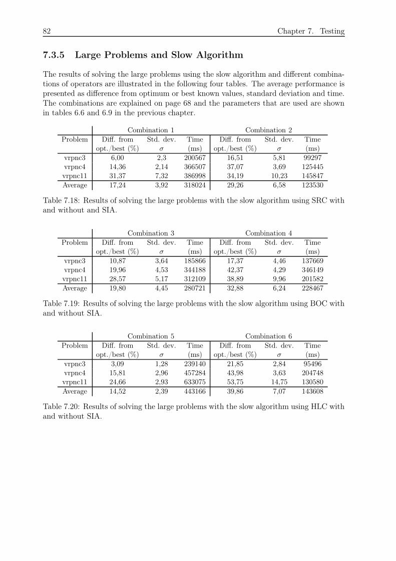
82 Chapter 7. Testing
7.3.5 Large Problems and Slow Algorithm
The results of solving the large problems using the slow algorithm and different combina-tions of operators are illustrated in the following four tables. The average performance ispresented as difference from optimum or best known values, standard deviation and time.The combinations are explained on page 68 and the parameters that are used are shownin tables 6.6 and 6.9 in the previous chapter.
Combination 1 Combination 2
Problem Diff. from Std. dev. Time Diff. from Std. dev. Timeopt./best (%) σ (ms) opt./best (%) σ (ms)
vrpnc3 6,00 2,3 200567 16,51 5,81 99297vrpnc4 14,36 2,14 366507 37,07 3,69 125445vrpnc11 31,37 7,32 386998 34,19 10,23 145847
Average 17,24 3,92 318024 29,26 6,58 123530
Table 7.18: Results of solving the large problems with the slow algorithm using SRC withand without and SIA.
Combination 3 Combination 4
Problem Diff. from Std. dev. Time Diff. from Std. dev. Timeopt./best (%) σ (ms) opt./best (%) σ (ms)
vrpnc3 10,87 3,64 185866 17,37 4,46 137669vrpnc4 19,96 4,53 344188 42,37 4,29 346149vrpnc11 28,57 5,17 312109 38,89 9,96 201582
Average 19,80 4,45 280721 32,88 6,24 228467
Table 7.19: Results of solving the large problems with the slow algorithm using BOC withand without SIA.
Combination 5 Combination 6
Problem Diff. from Std. dev. Time Diff. from Std. dev. Timeopt./best (%) σ (ms) opt./best (%) σ (ms)
vrpnc3 3,09 1,28 239140 21,85 2,84 95496vrpnc4 15,81 2,96 457284 43,98 3,63 204748vrpnc11 24,66 2,93 633075 53,75 14,75 130580
Average 14,52 2,39 443166 39,86 7,07 143608
Table 7.20: Results of solving the large problems with the slow algorithm using HLC withand without SIA.
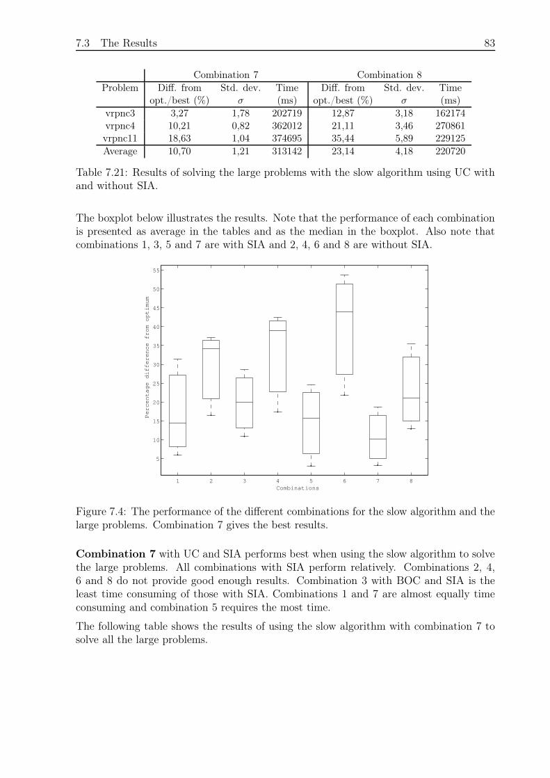
7.3 The Results 83
Combination 7 Combination 8
Problem Diff. from Std. dev. Time Diff. from Std. dev. Timeopt./best (%) σ (ms) opt./best (%) σ (ms)
vrpnc3 3,27 1,78 202719 12,87 3,18 162174vrpnc4 10,21 0,82 362012 21,11 3,46 270861vrpnc11 18,63 1,04 374695 35,44 5,89 229125
Average 10,70 1,21 313142 23,14 4,18 220720
Table 7.21: Results of solving the large problems with the slow algorithm using UC withand without SIA.
The boxplot below illustrates the results. Note that the performance of each combinationis presented as average in the tables and as the median in the boxplot. Also note thatcombinations 1, 3, 5 and 7 are with SIA and 2, 4, 6 and 8 are without SIA.
1 2 3 4 5 6 7 8
5
10
15
20
25
30
35
40
45
50
55
Percentage difference from optimum
Combinations
Figure 7.4: The performance of the different combinations for the slow algorithm and thelarge problems. Combination 7 gives the best results.
Combination 7 with UC and SIA performs best when using the slow algorithm to solvethe large problems. All combinations with SIA perform relatively. Combinations 2, 4,6 and 8 do not provide good enough results. Combination 3 with BOC and SIA is theleast time consuming of those with SIA. Combinations 1 and 7 are almost equally timeconsuming and combination 5 requires the most time.
The following table shows the results of using the slow algorithm with combination 7 tosolve all the large problems.
84 Chapter 7. Testing
Problem Diff. from Std. dev. Timeopt./best (%) σ (ms)
E-101-k8 4,91 2,55 226514F-n135-k7 17,98 3,36 537567G-n262-k25 9,13 1,28 1308962
vrpnc3 3,27 1,78 202719vrpnc4 10,21 0,82 362012vrpnc5 14,28 1,73 889969vrpnc11 18,63 1,04 374695
Average 11,20 1,79 557491
Table 7.22: Results of solving all the large problems with the slow algorithm using com-bination 7, i.e. UC and SIA.
7.3.6 Comparison of Fast and Slow Algorithm for Large Prob-
lems.
Combination 7 with UC and SIA performed best for both the fast algorithm and theslow algorithm. A comparison of the results of tables 7.17 and 7.22, shows that theslow algorithm performs better than the fast one. The difference in the performance isa little bit less than 6%. The slow algorithm is more time consuming. On average itrequires 557491 ms, which accounts for approximately 9,3 min. As before, accuracy isconsidered more important than computation time, as long as it is within reasonablelimits. Consequently, the slow algorithm with combination 7 is chosen for the largeproblems.
7.3.7 Comparison of the Algorithm and other Metaheuristics
Now it is time to compare the best algorithms that have been obtained in this projectto proposed results of the best metaheuristics. The slow algorithm with combination 1performed best for the small problems and the slow algorithm with combination 7 providedthe best results for the large problems. Hereafter, the algorithms will be referred to asSRC-GA and UC-GA, respectively.
In table 7.23 the final results are shown for 7 CMT problems. It was not the intentionof this project to focus specially on the CMT problems but the results of the best meta-heuristics are proposed by the means of these problems. The CMT problems are actually14. Those that are not in the following table also include maximum route time and a droptime for each customer. The algorithm of this project does not support these factors andthose problems are therefore eliminated.
The results of the Tabu Search heuristics Taburoute, Taillard and Adaptive memory arefrom [4]. They are explained shortly in section 2.1.4. The results of Taillard and Adaptivememory present the best performance of several runs. Information about the how the testswere made for Taburoute are missing. Although a comparison of the best performance ofseveral runs and the average performance of ten runs is really unfair, it gives a clue about
7.3 The Results 85
the efficiency of the algorithms of this project. Luckily, Berger and Barkaoui present in[2] the result of the Hybrid Genetic Algorithm (HGA-VRP) as an average performance.Although, the number of runs is not given. The algorithm is explained shortly in section2.1.4.
The results of SRC-GA for the small problems are taken from table 7.12 and the results ofUC-GA for the large problems are taken from table 7.22. Problems vrpnc1 and vrpnc12were used for parameter tuning. Usually, it is not preferable to present the results ofthe problems that were used for tuning. However, this is done here in order to make thecomparison based on more problems. Problem vrpnc1 was recalculated using SRC-GAand the results of vrpnc12 were obtained using UC-GA.
Taburoute Taillard Adaptive HGA-VRP SRC-GA andmemory UC-GA
Problem Perf. Time Perf. Perf. Perf. Time Perf. Time(%) (min) (%) (%) (%) (min) (%) (min)
vrpnc1 0,00 6,0 0,00 0,00 0,00 2,00 2,12 1,69vrpnc2 0,06 53,8 0,00 0,00 0,57 14,33 6,08 1,61vrpnc3 0,04 18,4 0,00 0,00 0,47 27,90 3,27 3,38vrpnc4 0,08 58,8 0,00 0,00 1,63 48,98 10,21 6,03vrpnc5 1,84 90,9 0,57 0,00 2,76 55,41 14,28 14,83vrpnc11 2,75 22,2 0,00 0,00 0,75 22,43 18,63 6,24vrpnc12 0,00 16,0 0,00 0,00 0,00 7,21 19,07 4,55Average 0,68 38,01 0,08 0,00 0,88 25,47 10,52 5,48
Table 7.23: Comparison of SRC-GA and UC-GA and proposed results of three TabuSearch heuristics and the Hybrid Genetic Algorithm. The results above the line areobtained using SRC-GA and the results below the line are from using UC-GA. AlgorithmsSRC-GA and UC-GA do not compete with the other metaheuristics.
The results in the table above illustrate that SRC-GA and UC-GA are outperformed bythe other metaheuristics. Even though the comparison is not perfectly reasonable, theresults are quite clear because the difference in the performance is rather large. TheHGA-VRP appears to be rather effective on average since its results are quite close tothe TS heuristics, which results propose their best performance. Of those algorithms thatpresent the time, SRC-GA and UC-GA are definitely faster with an average time that isabout 1
5of the time HGA-VRP requires.
Courdeau et al. [4] make an analysis of the three Tabu Search heuristics above, amongothers, in order to evaluate them in terms of accuracy, speed, simplicity and flexibility. Theresults are illustrated in table 7.24. An effort has been made to evaluate the algorithmsSRC-GA and UC-GA together and HGA-VRP as well, with the help of the results intable 7.23. The results can only be used for comparison, since they are mostly based onpersonal evaluation. The flexibility of HGA-VRP is left empty because its results are onlyillustrated for the CMT problems in [2].
86 Chapter 7. Testing
Taburoute Taillard Adaptive memory HGA-VRP SRC-GA/UC-GAAccuracy High Very high Very high High LowSpeed Medium Low Low Medium HighSimplicity Medium Medium-low Medium-low Medium HighFlexibility High High High ? High
Table 7.24: Evaluation of SRC-GA, UC-GA and other metaheuristics.
When it comes to accuracy neither SRC-GA nor UC-GA perform well enough. On theother hand, they score high on speed, simplicity and flexibility.
7.4 Summary
In this chapter the results of the testing have been illustrated. Combination 7 with UCand SIA turned out to be the best one for the fast algorithm when solving the smallproblems. For the slow algorithm, combination 1 with SRC and SIA gave the best resultsfor the small problems. The slow algorithm outperformed the fast one and was used forfurther comparison. Combination 7 provided the best results for both the fast and theslow algorithm when solving the large problems. The slow algorithm outperformed thefast one. The best algorithms for the small and the large problems were named SRC-GA and UC-GA and compared to current best metaheuristics. They were not accurateenough, but they were quite fast. In the next chapter the results are discussed.
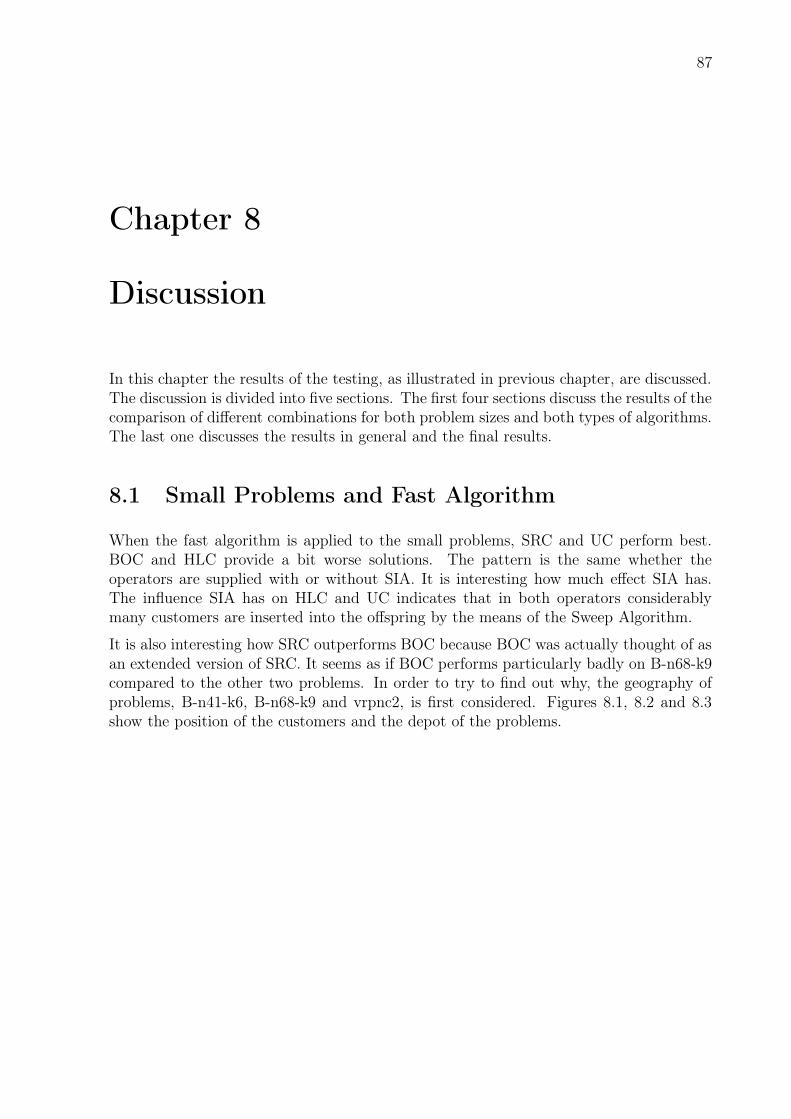
87
Chapter 8
Discussion
In this chapter the results of the testing, as illustrated in previous chapter, are discussed.The discussion is divided into five sections. The first four sections discuss the results of thecomparison of different combinations for both problem sizes and both types of algorithms.The last one discusses the results in general and the final results.
8.1 Small Problems and Fast Algorithm
When the fast algorithm is applied to the small problems, SRC and UC perform best.BOC and HLC provide a bit worse solutions. The pattern is the same whether theoperators are supplied with or without SIA. It is interesting how much effect SIA has.The influence SIA has on HLC and UC indicates that in both operators considerablymany customers are inserted into the offspring by the means of the Sweep Algorithm.
It is also interesting how SRC outperforms BOC because BOC was actually thought of asan extended version of SRC. It seems as if BOC performs particularly badly on B-n68-k9compared to the other two problems. In order to try to find out why, the geography ofproblems, B-n41-k6, B-n68-k9 and vrpnc2, is first considered. Figures 8.1, 8.2 and 8.3show the position of the customers and the depot of the problems.
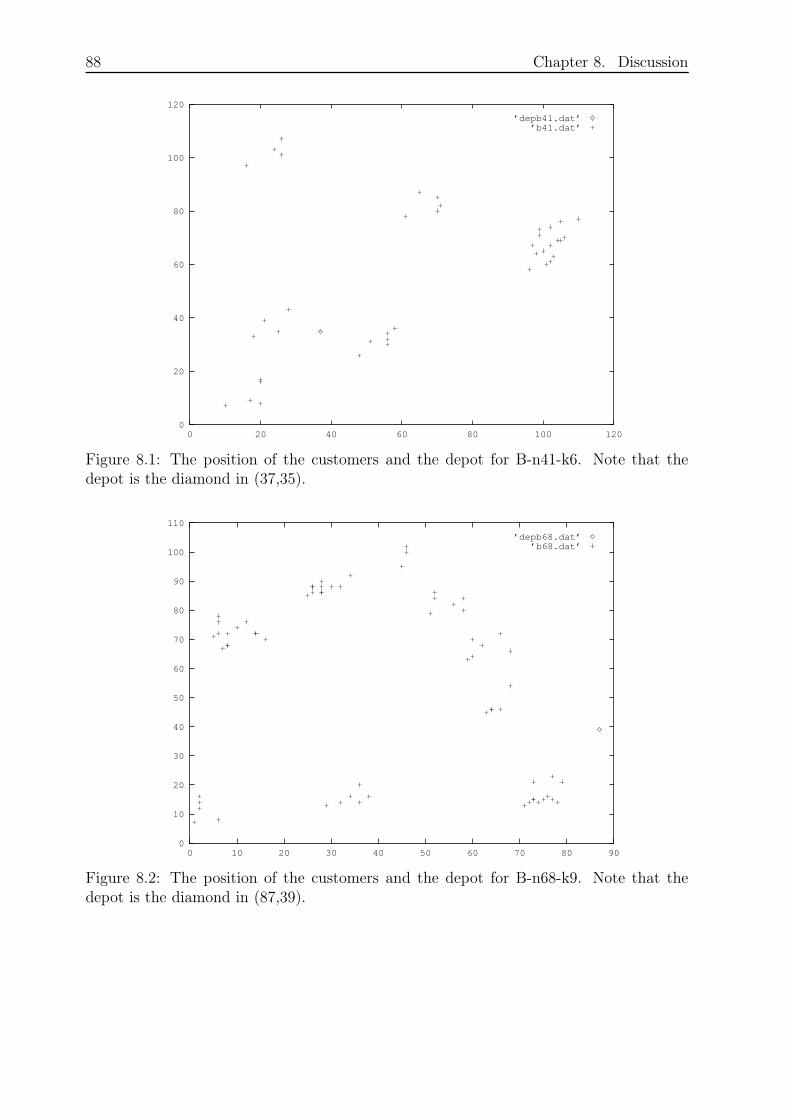
88 Chapter 8. Discussion
0
20
40
60
80
100
120
0 20 40 60 80 100 120
’depb41.dat’’b41.dat’
Figure 8.1: The position of the customers and the depot for B-n41-k6. Note that thedepot is the diamond in (37,35).
0
10
20
30
40
50
60
70
80
90
100
110
0 10 20 30 40 50 60 70 80 90
’depb68.dat’’b68.dat’
Figure 8.2: The position of the customers and the depot for B-n68-k9. Note that thedepot is the diamond in (87,39).
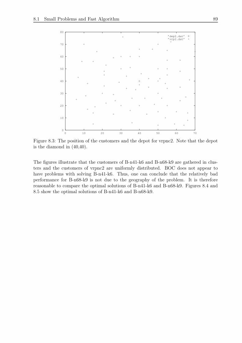
8.1 Small Problems and Fast Algorithm 89
0
10
20
30
40
50
60
70
80
0 10 20 30 40 50 60 70
’dep2.dat’’vrp2.dat’
Figure 8.3: The position of the customers and the depot for vrpnc2. Note that the depotis the diamond in (40,40).
The figures illustrate that the customers of B-n41-k6 and B-n68-k9 are gathered in clus-ters and the customers of vrpnc2 are uniformly distributed. BOC does not appear tohave problems with solving B-n41-k6. Thus, one can conclude that the relatively badperformance for B-n68-k9 is not due to the geography of the problem. It is thereforereasonable to compare the optimal solutions of B-n41-k6 and B-n68-k9. Figures 8.4 and8.5 show the optimal solutions of B-n41-k6 and B-n68-k9.
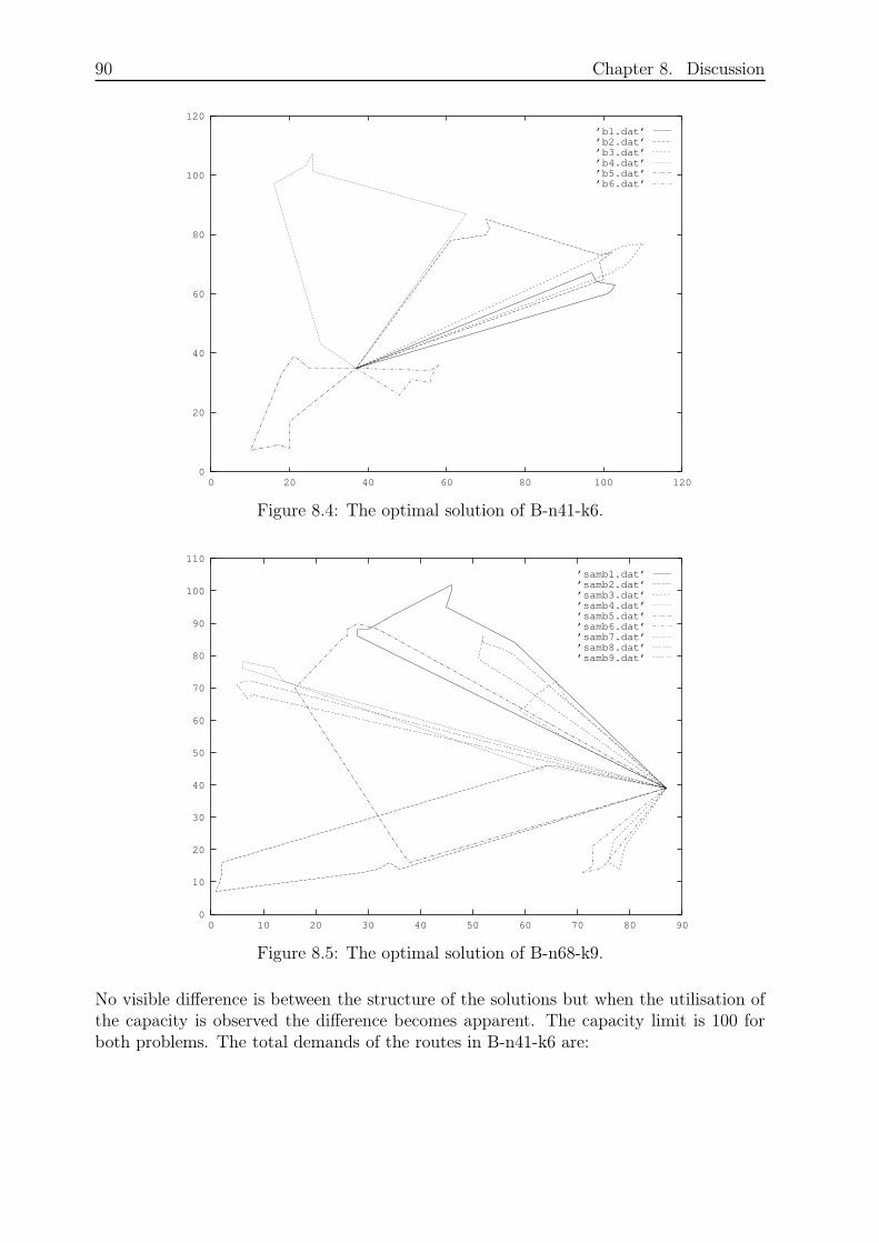
90 Chapter 8. Discussion
0
20
40
60
80
100
120
0 20 40 60 80 100 120
’b1.dat’’b2.dat’’b3.dat’’b4.dat’’b5.dat’’b6.dat’
Figure 8.4: The optimal solution of B-n41-k6.
0
10
20
30
40
50
60
70
80
90
100
110
0 10 20 30 40 50 60 70 80 90
’samb1.dat’’samb2.dat’’samb3.dat’’samb4.dat’’samb5.dat’’samb6.dat’’samb7.dat’’samb8.dat’’samb9.dat’
Figure 8.5: The optimal solution of B-n68-k9.
No visible difference is between the structure of the solutions but when the utilisation ofthe capacity is observed the difference becomes apparent. The capacity limit is 100 forboth problems. The total demands of the routes in B-n41-k6 are:
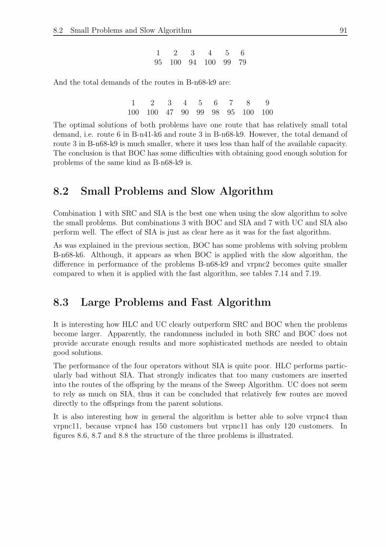
8.2 Small Problems and Slow Algorithm 91
1 2 3 4 5 695 100 94 100 99 79
And the total demands of the routes in B-n68-k9 are:
1 2 3 4 5 6 7 8 9100 100 47 90 99 98 95 100 100
The optimal solutions of both problems have one route that has relatively small totaldemand, i.e. route 6 in B-n41-k6 and route 3 in B-n68-k9. However, the total demand ofroute 3 in B-n68-k9 is much smaller, where it uses less than half of the available capacity.The conclusion is that BOC has some difficulties with obtaining good enough solution forproblems of the same kind as B-n68-k9 is.
8.2 Small Problems and Slow Algorithm
Combination 1 with SRC and SIA is the best one when using the slow algorithm to solvethe small problems. But combinations 3 with BOC and SIA and 7 with UC and SIA alsoperform well. The effect of SIA is just as clear here as it was for the fast algorithm.
As was explained in the previous section, BOC has some problems with solving problemB-n68-k6. Although, it appears as when BOC is applied with the slow algorithm, thedifference in performance of the problems B-n68-k9 and vrpnc2 becomes quite smallercompared to when it is applied with the fast algorithm, see tables 7.14 and 7.19.
8.3 Large Problems and Fast Algorithm
It is interesting how HLC and UC clearly outperform SRC and BOC when the problemsbecome larger. Apparently, the randomness included in both SRC and BOC does notprovide accurate enough results and more sophisticated methods are needed to obtaingood solutions.
The performance of the four operators without SIA is quite poor. HLC performs partic-ularly bad without SIA. That strongly indicates that too many customers are insertedinto the routes of the offspring by the means of the Sweep Algorithm. UC does not seemto rely as much on SIA, thus it can be concluded that relatively few routes are moveddirectly to the offsprings from the parent solutions.
It is also interesting how in general the algorithm is better able to solve vrpnc4 thanvrpnc11, because vrpnc4 has 150 customers but vrpnc11 has only 120 customers. Infigures 8.6, 8.7 and 8.8 the structure of the three problems is illustrated.
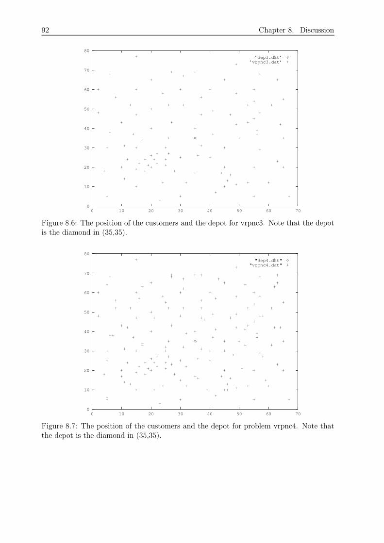
92 Chapter 8. Discussion
0
10
20
30
40
50
60
70
80
0 10 20 30 40 50 60 70
’dep3.dat’’vrpnc3.dat’
Figure 8.6: The position of the customers and the depot for vrpnc3. Note that the depotis the diamond in (35,35).
0
10
20
30
40
50
60
70
80
0 10 20 30 40 50 60 70
"dep4.dat""vrpnc4.dat"
Figure 8.7: The position of the customers and the depot for problem vrpnc4. Note thatthe depot is the diamond in (35,35).
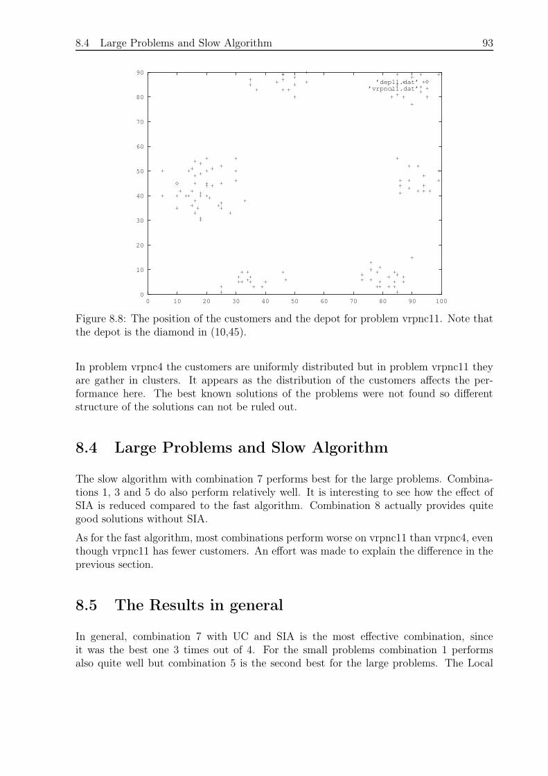
8.4 Large Problems and Slow Algorithm 93
0
10
20
30
40
50
60
70
80
90
0 10 20 30 40 50 60 70 80 90 100
’dep11.dat’’vrpnc11.dat’
Figure 8.8: The position of the customers and the depot for problem vrpnc11. Note thatthe depot is the diamond in (10,45).
In problem vrpnc4 the customers are uniformly distributed but in problem vrpnc11 theyare gather in clusters. It appears as the distribution of the customers affects the per-formance here. The best known solutions of the problems were not found so differentstructure of the solutions can not be ruled out.
8.4 Large Problems and Slow Algorithm
The slow algorithm with combination 7 performs best for the large problems. Combina-tions 1, 3 and 5 do also perform relatively well. It is interesting to see how the effect ofSIA is reduced compared to the fast algorithm. Combination 8 actually provides quitegood solutions without SIA.
As for the fast algorithm, most combinations perform worse on vrpnc11 than vrpnc4, eventhough vrpnc11 has fewer customers. An effort was made to explain the difference in theprevious section.
8.5 The Results in general
In general, combination 7 with UC and SIA is the most effective combination, sinceit was the best one 3 times out of 4. For the small problems combination 1 performsalso quite well but combination 5 is the second best for the large problems. The Local
94 Chapter 8. Discussion
Search algorithm SIA is essential to obtain an effective algorithm. The performance ofthe combinations without it is unacceptable. The overall performance of BOC is ratherbad.
Unfortunately, neither SRC-GA nor UC-GA are competitive to the best TS heuristics orthe HGA-VRP. The average performance of the algorithms together was 10,52% from theoptimum or best known values where the other metaheuristics are within 1%. Even thoughthe numbers for the TS heuristics are best of several runs it is estimated that differencein performance of 10% is too much for the algorithms to be considered competitive. Also,the results of HGA-VRP are average numbers of several runs and they are also within 1%from the optimum or best known values.
It is unfortunate that the results of the TS heuristics and HGA-VRP are only presentedby the means of the CMT problems. The algorithms SRC-GA and UC-GA is not adjustedparticularly to the CMT problems and they were tuned using other types of problems aswell. It is interesting to see how UC-GA performs relatively well on problem G-n262-k25,see table 7.22. That indicates that the algorithm does not become less effective as soonas the problems become larger.
In table 7.24 the heuristics are compared by the means of the criteria speed, simplicityand flexibility as well as accuracy. Even though the table is mostly based on personalevaluation, it shows that the algorithms have something to contribute, because it is rel-atively fast and moreover it is rather simple. Therefore, it would be very interesting tosee if some kind of a combination of HGA-VRP and UC with SIA would be promising.The idea of HGA-VRP was shortly introduced in section 2.1.4. It uses so-called parallelversion of GA, which generates a number of subpopulations that evolve independentlyusing a serial GA, like has been done here. Once in a while the subpopulations interact.HGA-VRP generates two subpopulations. For instance, in order to allow the algorithm toobtain good solutions for problems of similar type as B-n68-k9, different operators couldbe used for different populations. Using Geographical Merge on the one population andnot on the other will most likely help to obtain good solutions, where one route only usesa small part of the capacity. Therefore, an algorithm would be obtained, which is able toadapt to different problems with different kinds of optimal solutions.
8.6 Summary
In this chapter the results have been discussed. Combination 7 with UC with SIA hasprovided some promising results, particularly for the larger problems. Although, theresults are not quite competitive with proposed results of TS heuristics and the HybridGenetic Algorithm. For further work, a combination of HGA-VRP and UC with SIA issuggested. In the next chapter the conclusion in presented.
95
Chapter 9
Conclusion
The aim of this project was to design an efficient Genetic Algorithm in order to solvethe Capacitated Vehicle Routing Problem (VRP). A program was developed based ona smaller program, with rather simple crossover and mutation operators, named SimpleRandom Crossover and Simple Random Mutation. That program was designed by theauthor and Hildur Ólafsdóttir in the course Large-Scale Optimisation at DTU in thespring of 2003.
At first, three Local Search Algorithms were designed and implemented, in order to im-prove single routes in the VRP, one at a time. The algorithms were named Simple Ran-dom Algorithm, Non Repeating Algorithm and Steepest Improvement Algorithm. Thealgorithms were compared based on 10 TSP problems with up to 50 customers. Sim-ple Random Algorithm performed worst by far. The average difference from optimumwas 88,40±37,78%. Non Repeating Algorithm and Steepest Improvement Algorithm pro-vided good results or 5,27±2,81% and 4,86±2,97% from optimum. Steepest ImprovementAlgorithm was chosen for further use.
Three new crossover operators were developed; Biggest Overlap Crossover, HorizontalLine Crossover and Uniform Crossover. In different ways, they all focus on the geogra-phy of the problem, in order to try to provide good results. In the development process,some drawbacks of the crossover operators were discovered. Therefore, two supportingoperators were made. Repairing Operator was designed for Simple Random Crossoverand Biggest Overlap Crossover, and for Horizontal Line Crossover and Uniform CrossoverGeographical Merge was developed. Eight combinations of operators were defined. Twocombinations for each crossover operator, with and without Steepest Improvement Algo-rithm.
The test problems were divided into small problems defined as having less than 100 cus-tomers and large problems with 100 customers or more. Additionally, a fast algorithmwith 10000 iterations and relatively small populations and a slow algorithm using 100000iterations and larger population were defined. For both the small and the large problems,the combinations of operators were compared using both fast and slow algorithm. Threetest problems of each size were used. When the fast algorithm was used to solve the smallproblems, combination 7 with Uniform Crossover and Steepest Improvement Algorithms
96 Chapter 9. Conclusion
performed best. The difference from optimum or best known values was 11,28±3,48%.Combination 1 with Simple Random Crossover and Steepest Improvement provided thebest results when the slow algorithm was used to solve the small problems. The resultswere 4,17±1,49% from the optimum or best know values. For the large problems, combina-tion 7 gave the best results when using the fast algorithm. That resulted in 16,36±2,17%from best known values. When the slow algorithm was used for the large problems, thebest results were again obtained by combination 7. The difference from best known valueswas 10,70±1,21%.
For each size, a choice was made between the fast and the slow algorithm. The algorithmsfor the small problems were applied to additional 9 problems and the algorithms for thelarge problems were applied to additional 4 problems. (Thus the testing was made with12 small problems and 7 large problems.) For the small problems, the fast algorithmwas 11,37±3,17% from the optimal or best known values and the slow algorithm was4,16±1,22%. Furthermore, the fast algorithm was 17,17±2,46% from the optimal or bestknow values and the slow one was 11,20±1,79%, for the large problems. Thus, the slowalgorithm with combination 1 was chosen for the small problems and the slow algorithmwith combination 7 was chosen for the large problems. The algorithm for the smallproblems was called SRC-GA and the algorithm for the large problems was called UC-GA.
The following hypothesis was stated in chapter 1:
It is possible to develop operators for Genetic Algorithms efficient enough to solve large
Vehicle Routing Problems.
In order to verify the hypothesis, SRC-GA and UC-GA were compared to the HybridGenetic Algorithm (HGA-VRP) and three Tabu Search heuristics: Taburoute, Taillard’sAlgorithm and Adaptive memory. These heuristics have proposed good results on prob-lems referred to as the Christofides, Mingozzi and Toth problems. The comparison wasbased on the results of 7 problems. Taburoute, Taillard’s Algorithm and Adaptive mem-ory were 0,68, 0,08 and 0,00% from optimum or best known values and HGA-VRP was0,88%. The results of Taburoute, Taillard’s Algorithm and Adaptive memory are thebest from several runs but the results of HGA-VRP are average results of several runs.Together SRC-GA and UC-GA did not provide good enough results on these problems,with an average performance of 10,52%. Thus the hypothesis was rejected.
However, SRC-GA and UC-GA are on average considerably faster than the other heuristicsand more importantly they present some very simple operators. Furthermore, they arerather flexible. For further work focusing on large problems, it could be very interesting tomake some other hybrid genetic algorithm with Uniform Crossover and the correspondingoperators. That would result in an algorithm with a simple crossover and a numberof subpopulations that are each maintained parallel instead of serial, as was done here.Hopefully, it would be able to provide relatively good results more quickly, compared tothe one presented in this project.
97
Bibliography
[1] E. Aarts and J. K. Lenstra. Local Search in Combinatorial Optimization. Springer-Verlag, 1996.
[2] J. Berger and M. Barkaoui. A new hybrid genetic algorithm for the capacitatedvehicle routing problem. Journal of the Operational Research Society, 41(2):179–194,2003.
[3] Charles Darwin. Britannica concise encyclopedia from encyclopædia britannica.,2004. URL http://concise.britannica.com/ebc/article?eu=387589.
[4] J-F. Cordeau, M. Gendreau, G. Laporte, J-Y. Potvin, and F. Semet. A guide tovehicle routing heuristics. Journal of the Operational Research Society, 53:512–522,2002.
[5] Evolutionary Algorithms. Lecture slides: Evolutionary algorithms, 2004. URL http:
//www.imm.dtu.dk/courses/02715/.[6] E. Falkenauer. A hybrid grouping genetic algorithm for bin packing. Journal of
Heuristics, 2:5–30, 1996.[7] M. Fisher. Vehicle routing. Handbooks of Operations Research and Management
Science, chapter 1, 8:1–31, 1995.[8] M. Gendreau, A. Hertz, and G. Laporte. New insertion and postoptimization proce-
dures for the traveling salesman problem. Operations Research, 40:1086–1094, 1994.[9] M. Gendreau, A. Hertz, and G. Laporte. A tabu search heuristic for the vehicle
routing problem. Management Science, 40:1276–1290, 1994.[10] M. Gendreau, G. Laporte, and J-Y. Potvin. Metaheuristics for the vehicle routing
problem. Technical Report G-98-52, GERAD, 1999.[11] M. Jünger, G. Reinelt, and G. Rinaldi. The travelling salesman problem. Handbooks
of Operations Research and Management Science, chapter 4, 7:225–330, 1995.[12] G. Laporte, M. Gendreau, J-Y. Potvin, and F. Semet. Classical and modern heuristics
for the vehicle routing problem. International Transactions in Operational Research,7:285–300, 2000.
[13] G. Laporte and F. Semet. Classical heuristics for the vehicle routing problem. Tech-nical Report G-98-54, GERAD, 1999.
[14] Z. Michalewicz, editor. Genetic Algorithm + Data Structures = Evolution Programs,3rd, revised and extended edition. Springer-Verlag, 1996.
[15] F.B. Pereira, J. Tavares, P. Machado, and E. Costa. GVR: a new genetic represen-tation for the vehicle routing problem. Prodeedings of the 13th Irish InternationalConference on Artificial Intelligence and Cognitive Science, pages 95–102, 2002.
[16] S.M. Sait and H. Youssef, editors. Iterative Computer Algorithms with Application

98 BIBLIOGRAPHY
in Engineering: Solving Combinatorial Optimization Problems, chapter 3. IEEEComputer Society, 1999.
[17] The VRP Web. The vrp web, 2004. URL http://neo.lcc.uma.es/radi-aeb/
WebVRP/index.html?/results/BestResults.h%tm.[18] Thomas Stidsen. Thomas stidsen, 2003. URL [email protected].[19] TSPLIB. Tsplib, 2001. URL http://www.iwr.uni-heidelberg.de/groups/
comopt/software/TSPLIB95/.[20] Vehicle Routing Data Sets. Vehicle routing data sets, 2003. URL http://
branchandcut.org/VRP/data/.[21] L.A. Wolsey, editor. Integer Programming. John Wiley and Sons, 1998.[22] A.H. Wright and J.E. Rowe. Continuous dynamical system models of steady-state
genetic algorithms. Foundations of Genetic Algorithms, 6:209–226, 2001.
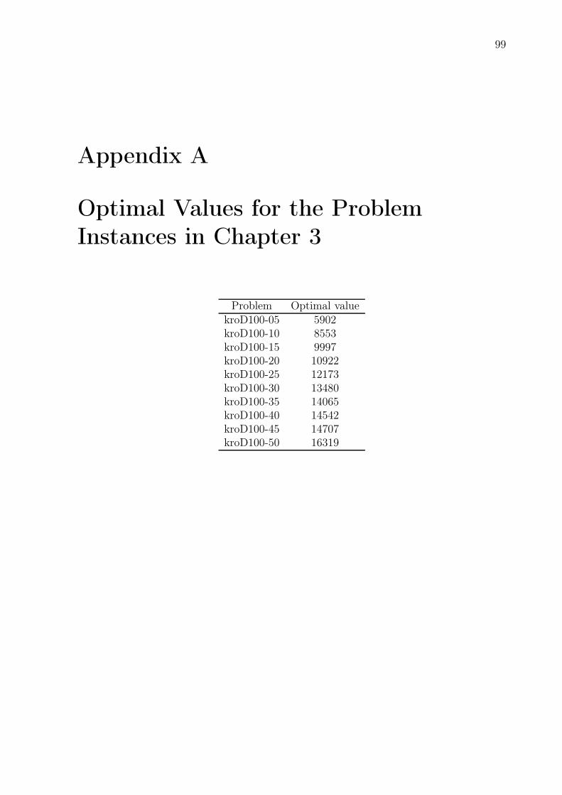
99
Appendix A
Optimal Values for the Problem
Instances in Chapter 3
Problem Optimal valuekroD100-05 5902kroD100-10 8553kroD100-15 9997kroD100-20 10922kroD100-25 12173kroD100-30 13480kroD100-35 14065kroD100-40 14542kroD100-45 14707kroD100-50 16319

100 Appendix A. Optimal Values for the Problem Instances in Chapter 3
101
Appendix B
Results of Testing of Repairing
Operator in Chapter 4
B.1 Simple Random Crossover
Difference from optimumProblem Diff. from Diff. from Diff. from Diff. from
sizes optimum (%) optimum (%) optimum (%) optimum (%)32 8,21 23,33 33,49 31,5344 5.84 17.78 20.5 29.6860 6.2 18.08 23.63 29.1380 5.84 14.92 23.59 27.9
Average 6,52 18,53 25,30 29,56
Standard deviationProblem Std. dev. Std. dev. Std. dev. Std. dev.
sizes σ σ σ σ32 4,45 5,5 6,17 5,0144 1,38 2,38 3,62 6,1660 1.69 4,08 4,26 4,4180 1,74 5,26 7,13 3,98
Average 2,32 4,31 5,30 4,89
102 Appendix B. Results of Testing of Repairing Operator in Chapter 4
B.2 Biggest Crossover Operator
Difference from optimumProblem Diff. from Diff. from Diff. from Diff. from
sizes optimum (%) optimum (%) optimum (%) optimum (%)32 11,76 22,39 26,99 34,4244 6,56 18,85 23,5 32,3360 6,71 20,41 22,3 32,4880 10,03 18,23 25,92 32,66
Average 8,77 19,97 24,68 32,97
Standard deviationProblem Std. dev. Std. dev. Std. dev. Std. dev.
sizes σ σ σ σ32 7,95 4,42 4,58 4,7344 3,05 6,64 3,04 2,1260 4,29 5,24 5,88 3,7480 1,85 3,79 3,96 1,95
Average 4,29 5,02 4,37 3,14
103
Appendix C
Results of Parameter Tuning
C.1 Combination 1, SRC, SRM, RO and SIA
C.1.1 Small and Fast
A-n32-k5.vrp, M=50, IT=10000
Mutation \ Repair 0 50 100 2000 15,48 11,56 9,62 5,28 5,94 1,39 5,66 0,850 5,99 1,6 3,14 2,19 5,89 0,51 3,47 2,3100 4,8 4,08 5,15 2,19 3,42 2,26 3,9 2,64200 14,52 4,52 8,88 2,31 6,91 1,4 6,48 3
A-n32-k5.vrp, M=100, IT=10000
Mutation \ Repair 0 50 100 2000 13,57 3,21 6,76 2,44 5,79 3,39 5,36 2,5750 8,65 6,76 4,29 1,86 4,21 2,21 3,93 2,26100 6,51 0,67 5,1 1,79 4,72 2,3 5,84 0,1200 10,59 3,62 6,35 1,7 6,63 1,34 6,33 2,25
A-n32-k5.vrp, M=200, IT=10000
104 Appendix C. Results of Parameter Tuning
Mutation \ Repair 0 50 100 2000 13,62 8,85 4,06 2,32 5,77 0,69 5,92 1,0650 7,14 3,85 4,59 1,78 5,69 2,38 2,7 1,98100 9,64 3,93 3,9 3 3,39 2,37 3,06 2,34200 22,32 5,45 9,95 2,32 7,76 5,77 7,53 3,25
vrpcn1, M=50, IT=10000
Mutation \ Repair 0 50 100 2000 44,51 8,07 16,63 3,89 15,3 0,9 7,94 3,1250 14,98 8,82 11,37 5,39 7,49 4,09 10,54 4,82100 23,43 13,81 13,46 4,27 10,6 5,46 7,3 5,15200 18,86 5,52 12,38 3,5 21,71 6,12 12,25 2,61
vrpcn1, M=100, IT=10000
Mutation \ Repair 0 50 100 2000 25,84 23,69 8,44 5,47 8,89 1,86 12,44 6,1650 11,3 1,68 9,78 3,85 8,95 2,02 6,1 1,79100 10,41 1,47 14,67 6,06 7,17 2,8 5,97 1,51200 22,98 2,79 13,84 1,44 18,48 3,16 20,19 5,93
vrpcn1, M=200, IT=10000
Mutation \ Repair 0 50 100 2000 30,22 17,81 11,87 4,63 9,33 4,82 6,16 0,7250 17,59 4,98 11,37 2,11 12,06 1,82 8,63 3,86100 18,1 0,87 8,95 3,97 10,48 1,48 14,41 7,35200 30,16 3,38 20,89 1,4 22,86 2,57 19,94 1,8
C.1.2 Small and Slow
A-n32-k5.vrp, M=200, IT=100000
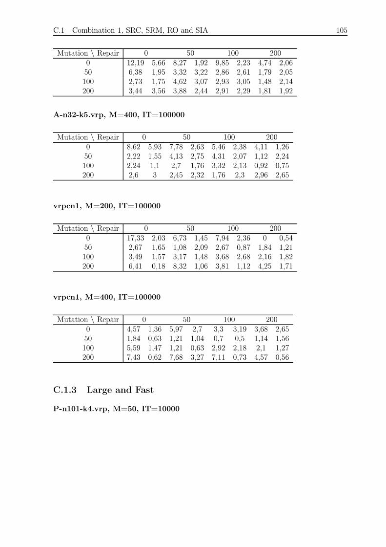
C.1 Combination 1, SRC, SRM, RO and SIA 105
Mutation \ Repair 0 50 100 2000 12,19 5,66 8,27 1,92 9,85 2,23 4,74 2,0650 6,38 1,95 3,32 3,22 2,86 2,61 1,79 2,05100 2,73 1,75 4,62 3,07 2,93 3,05 1,48 2,14200 3,44 3,56 3,88 2,44 2,91 2,29 1,81 1,92
A-n32-k5.vrp, M=400, IT=100000
Mutation \ Repair 0 50 100 2000 8,62 5,93 7,78 2,63 5,46 2,38 4,11 1,2650 2,22 1,55 4,13 2,75 4,31 2,07 1,12 2,24100 2,24 1,1 2,7 1,76 3,32 2,13 0,92 0,75200 2,6 3 2,45 2,32 1,76 2,3 2,96 2,65
vrpcn1, M=200, IT=100000
Mutation \ Repair 0 50 100 2000 17,33 2,03 6,73 1,45 7,94 2,36 0 0,5450 2,67 1,65 1,08 2,09 2,67 0,87 1,84 1,21100 3,49 1,57 3,17 1,48 3,68 2,68 2,16 1,82200 6,41 0,18 8,32 1,06 3,81 1,12 4,25 1,71
vrpcn1, M=400, IT=100000
Mutation \ Repair 0 50 100 2000 4,57 1,36 5,97 2,7 3,3 3,19 3,68 2,6550 1,84 0,63 1,21 1,04 0,7 0,5 1,14 1,56100 5,59 1,47 1,21 0,63 2,92 2,18 2,1 1,27200 7,43 0,62 7,68 3,27 7,11 0,73 4,57 0,56
C.1.3 Large and Fast
P-n101-k4.vrp, M=50, IT=10000
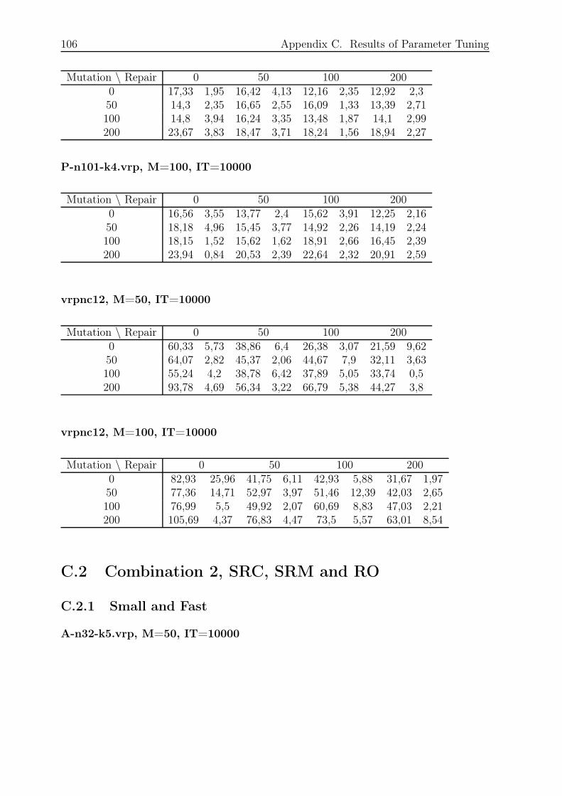
106 Appendix C. Results of Parameter Tuning
Mutation \ Repair 0 50 100 2000 17,33 1,95 16,42 4,13 12,16 2,35 12,92 2,350 14,3 2,35 16,65 2,55 16,09 1,33 13,39 2,71100 14,8 3,94 16,24 3,35 13,48 1,87 14,1 2,99200 23,67 3,83 18,47 3,71 18,24 1,56 18,94 2,27
P-n101-k4.vrp, M=100, IT=10000
Mutation \ Repair 0 50 100 2000 16,56 3,55 13,77 2,4 15,62 3,91 12,25 2,1650 18,18 4,96 15,45 3,77 14,92 2,26 14,19 2,24100 18,15 1,52 15,62 1,62 18,91 2,66 16,45 2,39200 23,94 0,84 20,53 2,39 22,64 2,32 20,91 2,59
vrpnc12, M=50, IT=10000
Mutation \ Repair 0 50 100 2000 60,33 5,73 38,86 6,4 26,38 3,07 21,59 9,6250 64,07 2,82 45,37 2,06 44,67 7,9 32,11 3,63100 55,24 4,2 38,78 6,42 37,89 5,05 33,74 0,5200 93,78 4,69 56,34 3,22 66,79 5,38 44,27 3,8
vrpnc12, M=100, IT=10000
Mutation \ Repair 0 50 100 2000 82,93 25,96 41,75 6,11 42,93 5,88 31,67 1,9750 77,36 14,71 52,97 3,97 51,46 12,39 42,03 2,65100 76,99 5,5 49,92 2,07 60,69 8,83 47,03 2,21200 105,69 4,37 76,83 4,47 73,5 5,57 63,01 8,54
C.2 Combination 2, SRC, SRM and RO
C.2.1 Small and Fast
A-n32-k5.vrp, M=50, IT=10000
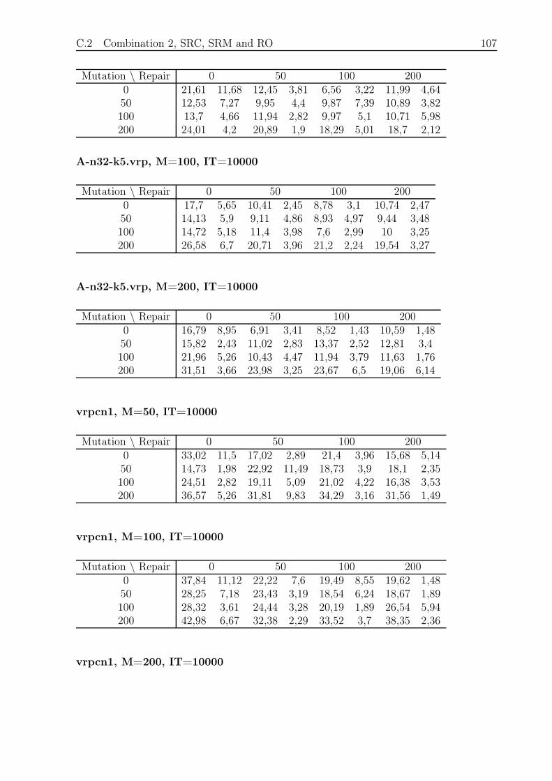
C.2 Combination 2, SRC, SRM and RO 107
Mutation \ Repair 0 50 100 2000 21,61 11,68 12,45 3,81 6,56 3,22 11,99 4,6450 12,53 7,27 9,95 4,4 9,87 7,39 10,89 3,82100 13,7 4,66 11,94 2,82 9,97 5,1 10,71 5,98200 24,01 4,2 20,89 1,9 18,29 5,01 18,7 2,12
A-n32-k5.vrp, M=100, IT=10000
Mutation \ Repair 0 50 100 2000 17,7 5,65 10,41 2,45 8,78 3,1 10,74 2,4750 14,13 5,9 9,11 4,86 8,93 4,97 9,44 3,48100 14,72 5,18 11,4 3,98 7,6 2,99 10 3,25200 26,58 6,7 20,71 3,96 21,2 2,24 19,54 3,27
A-n32-k5.vrp, M=200, IT=10000
Mutation \ Repair 0 50 100 2000 16,79 8,95 6,91 3,41 8,52 1,43 10,59 1,4850 15,82 2,43 11,02 2,83 13,37 2,52 12,81 3,4100 21,96 5,26 10,43 4,47 11,94 3,79 11,63 1,76200 31,51 3,66 23,98 3,25 23,67 6,5 19,06 6,14
vrpcn1, M=50, IT=10000
Mutation \ Repair 0 50 100 2000 33,02 11,5 17,02 2,89 21,4 3,96 15,68 5,1450 14,73 1,98 22,92 11,49 18,73 3,9 18,1 2,35100 24,51 2,82 19,11 5,09 21,02 4,22 16,38 3,53200 36,57 5,26 31,81 9,83 34,29 3,16 31,56 1,49
vrpcn1, M=100, IT=10000
Mutation \ Repair 0 50 100 2000 37,84 11,12 22,22 7,6 19,49 8,55 19,62 1,4850 28,25 7,18 23,43 3,19 18,54 6,24 18,67 1,89100 28,32 3,61 24,44 3,28 20,19 1,89 26,54 5,94200 42,98 6,67 32,38 2,29 33,52 3,7 38,35 2,36
vrpcn1, M=200, IT=10000
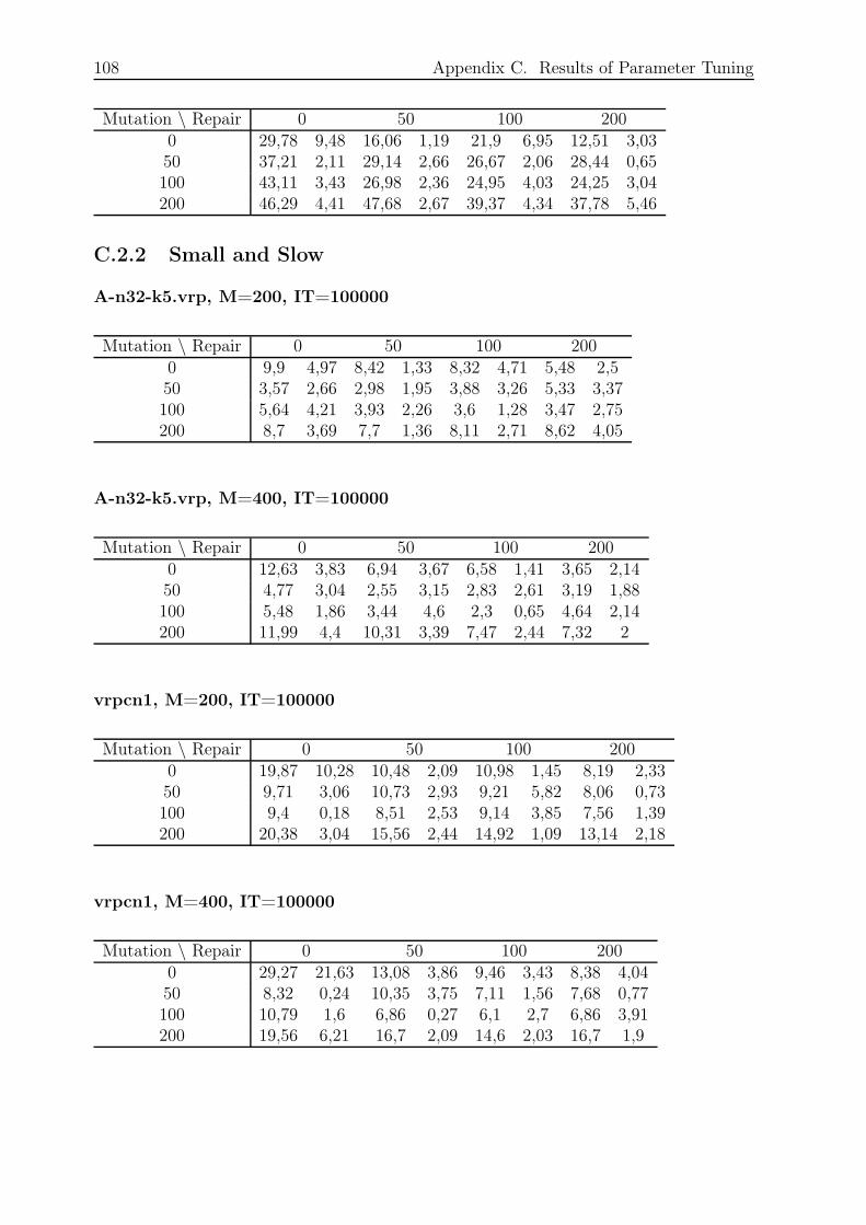
108 Appendix C. Results of Parameter Tuning
Mutation \ Repair 0 50 100 2000 29,78 9,48 16,06 1,19 21,9 6,95 12,51 3,0350 37,21 2,11 29,14 2,66 26,67 2,06 28,44 0,65100 43,11 3,43 26,98 2,36 24,95 4,03 24,25 3,04200 46,29 4,41 47,68 2,67 39,37 4,34 37,78 5,46
C.2.2 Small and Slow
A-n32-k5.vrp, M=200, IT=100000
Mutation \ Repair 0 50 100 2000 9,9 4,97 8,42 1,33 8,32 4,71 5,48 2,550 3,57 2,66 2,98 1,95 3,88 3,26 5,33 3,37100 5,64 4,21 3,93 2,26 3,6 1,28 3,47 2,75200 8,7 3,69 7,7 1,36 8,11 2,71 8,62 4,05
A-n32-k5.vrp, M=400, IT=100000
Mutation \ Repair 0 50 100 2000 12,63 3,83 6,94 3,67 6,58 1,41 3,65 2,1450 4,77 3,04 2,55 3,15 2,83 2,61 3,19 1,88100 5,48 1,86 3,44 4,6 2,3 0,65 4,64 2,14200 11,99 4,4 10,31 3,39 7,47 2,44 7,32 2
vrpcn1, M=200, IT=100000
Mutation \ Repair 0 50 100 2000 19,87 10,28 10,48 2,09 10,98 1,45 8,19 2,3350 9,71 3,06 10,73 2,93 9,21 5,82 8,06 0,73100 9,4 0,18 8,51 2,53 9,14 3,85 7,56 1,39200 20,38 3,04 15,56 2,44 14,92 1,09 13,14 2,18
vrpcn1, M=400, IT=100000
Mutation \ Repair 0 50 100 2000 29,27 21,63 13,08 3,86 9,46 3,43 8,38 4,0450 8,32 0,24 10,35 3,75 7,11 1,56 7,68 0,77100 10,79 1,6 6,86 0,27 6,1 2,7 6,86 3,91200 19,56 6,21 16,7 2,09 14,6 2,03 16,7 1,9
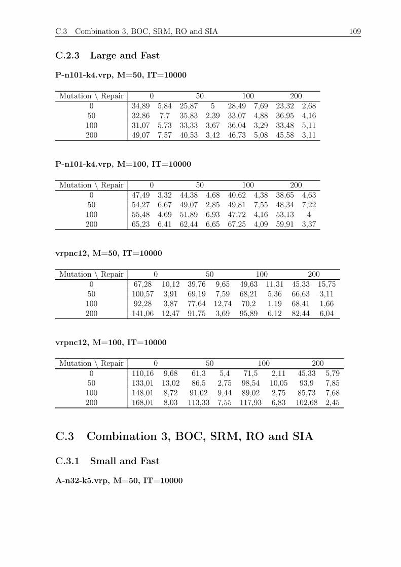
C.3 Combination 3, BOC, SRM, RO and SIA 109
C.2.3 Large and Fast
P-n101-k4.vrp, M=50, IT=10000
Mutation \ Repair 0 50 100 2000 34,89 5,84 25,87 5 28,49 7,69 23,32 2,6850 32,86 7,7 35,83 2,39 33,07 4,88 36,95 4,16100 31,07 5,73 33,33 3,67 36,04 3,29 33,48 5,11200 49,07 7,57 40,53 3,42 46,73 5,08 45,58 3,11
P-n101-k4.vrp, M=100, IT=10000
Mutation \ Repair 0 50 100 2000 47,49 3,32 44,38 4,68 40,62 4,38 38,65 4,6350 54,27 6,67 49,07 2,85 49,81 7,55 48,34 7,22100 55,48 4,69 51,89 6,93 47,72 4,16 53,13 4200 65,23 6,41 62,44 6,65 67,25 4,09 59,91 3,37
vrpnc12, M=50, IT=10000
Mutation \ Repair 0 50 100 2000 67,28 10,12 39,76 9,65 49,63 11,31 45,33 15,7550 100,57 3,91 69,19 7,59 68,21 5,36 66,63 3,11100 92,28 3,87 77,64 12,74 70,2 1,19 68,41 1,66200 141,06 12,47 91,75 3,69 95,89 6,12 82,44 6,04
vrpnc12, M=100, IT=10000
Mutation \ Repair 0 50 100 2000 110,16 9,68 61,3 5,4 71,5 2,11 45,33 5,7950 133,01 13,02 86,5 2,75 98,54 10,05 93,9 7,85100 148,01 8,72 91,02 9,44 89,02 2,75 85,73 7,68200 168,01 8,03 113,33 7,55 117,93 6,83 102,68 2,45
C.3 Combination 3, BOC, SRM, RO and SIA
C.3.1 Small and Fast
A-n32-k5.vrp, M=50, IT=10000
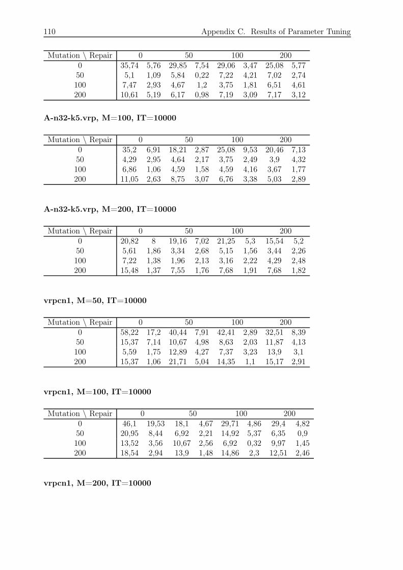
110 Appendix C. Results of Parameter Tuning
Mutation \ Repair 0 50 100 2000 35,74 5,76 29,85 7,54 29,06 3,47 25,08 5,7750 5,1 1,09 5,84 0,22 7,22 4,21 7,02 2,74100 7,47 2,93 4,67 1,2 3,75 1,81 6,51 4,61200 10,61 5,19 6,17 0,98 7,19 3,09 7,17 3,12
A-n32-k5.vrp, M=100, IT=10000
Mutation \ Repair 0 50 100 2000 35,2 6,91 18,21 2,87 25,08 9,53 20,46 7,1350 4,29 2,95 4,64 2,17 3,75 2,49 3,9 4,32100 6,86 1,06 4,59 1,58 4,59 4,16 3,67 1,77200 11,05 2,63 8,75 3,07 6,76 3,38 5,03 2,89
A-n32-k5.vrp, M=200, IT=10000
Mutation \ Repair 0 50 100 2000 20,82 8 19,16 7,02 21,25 5,3 15,54 5,250 5,61 1,86 3,34 2,68 5,15 1,56 3,44 2,26100 7,22 1,38 1,96 2,13 3,16 2,22 4,29 2,48200 15,48 1,37 7,55 1,76 7,68 1,91 7,68 1,82
vrpcn1, M=50, IT=10000
Mutation \ Repair 0 50 100 2000 58,22 17,2 40,44 7,91 42,41 2,89 32,51 8,3950 15,37 7,14 10,67 4,98 8,63 2,03 11,87 4,13100 5,59 1,75 12,89 4,27 7,37 3,23 13,9 3,1200 15,37 1,06 21,71 5,04 14,35 1,1 15,17 2,91
vrpcn1, M=100, IT=10000
Mutation \ Repair 0 50 100 2000 46,1 19,53 18,1 4,67 29,71 4,86 29,4 4,8250 20,95 8,44 6,92 2,21 14,92 5,37 6,35 0,9100 13,52 3,56 10,67 2,56 6,92 0,32 9,97 1,45200 18,54 2,94 13,9 1,48 14,86 2,3 12,51 2,46
vrpcn1, M=200, IT=10000
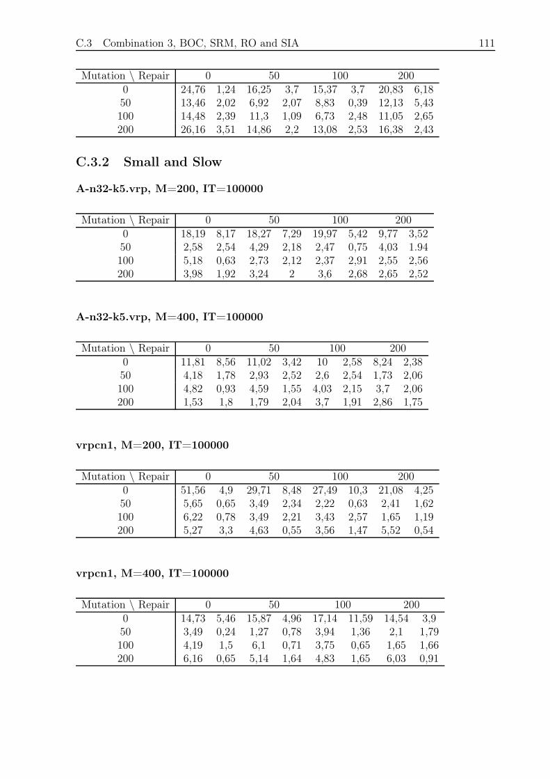
C.3 Combination 3, BOC, SRM, RO and SIA 111
Mutation \ Repair 0 50 100 2000 24,76 1,24 16,25 3,7 15,37 3,7 20,83 6,1850 13,46 2,02 6,92 2,07 8,83 0,39 12,13 5,43100 14,48 2,39 11,3 1,09 6,73 2,48 11,05 2,65200 26,16 3,51 14,86 2,2 13,08 2,53 16,38 2,43
C.3.2 Small and Slow
A-n32-k5.vrp, M=200, IT=100000
Mutation \ Repair 0 50 100 2000 18,19 8,17 18,27 7,29 19,97 5,42 9,77 3,5250 2,58 2,54 4,29 2,18 2,47 0,75 4,03 1.94100 5,18 0,63 2,73 2,12 2,37 2,91 2,55 2,56200 3,98 1,92 3,24 2 3,6 2,68 2,65 2,52
A-n32-k5.vrp, M=400, IT=100000
Mutation \ Repair 0 50 100 2000 11,81 8,56 11,02 3,42 10 2,58 8,24 2,3850 4,18 1,78 2,93 2,52 2,6 2,54 1,73 2,06100 4,82 0,93 4,59 1,55 4,03 2,15 3,7 2,06200 1,53 1,8 1,79 2,04 3,7 1,91 2,86 1,75
vrpcn1, M=200, IT=100000
Mutation \ Repair 0 50 100 2000 51,56 4,9 29,71 8,48 27,49 10,3 21,08 4,2550 5,65 0,65 3,49 2,34 2,22 0,63 2,41 1,62100 6,22 0,78 3,49 2,21 3,43 2,57 1,65 1,19200 5,27 3,3 4,63 0,55 3,56 1,47 5,52 0,54
vrpcn1, M=400, IT=100000
Mutation \ Repair 0 50 100 2000 14,73 5,46 15,87 4,96 17,14 11,59 14,54 3,950 3,49 0,24 1,27 0,78 3,94 1,36 2,1 1,79100 4,19 1,5 6,1 0,71 3,75 0,65 1,65 1,66200 6,16 0,65 5,14 1,64 4,83 1,65 6,03 0,91
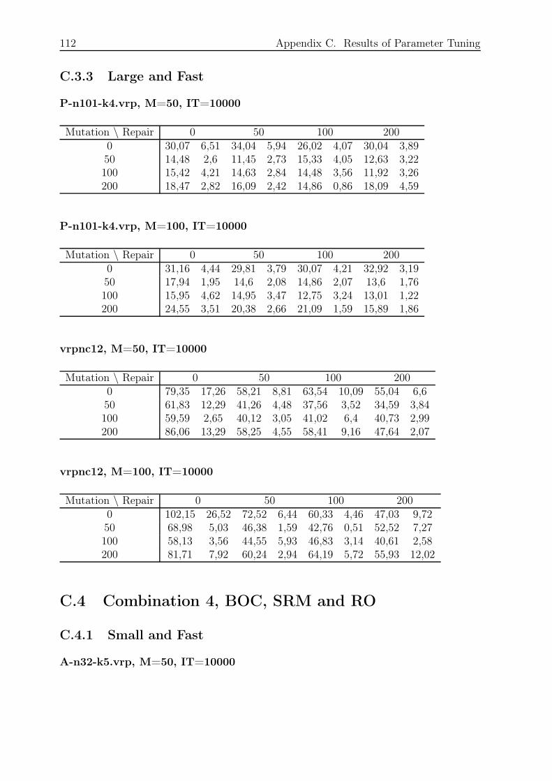
112 Appendix C. Results of Parameter Tuning
C.3.3 Large and Fast
P-n101-k4.vrp, M=50, IT=10000
Mutation \ Repair 0 50 100 2000 30,07 6,51 34,04 5,94 26,02 4,07 30,04 3,8950 14,48 2,6 11,45 2,73 15,33 4,05 12,63 3,22100 15,42 4,21 14,63 2,84 14,48 3,56 11,92 3,26200 18,47 2,82 16,09 2,42 14,86 0,86 18,09 4,59
P-n101-k4.vrp, M=100, IT=10000
Mutation \ Repair 0 50 100 2000 31,16 4,44 29,81 3,79 30,07 4,21 32,92 3,1950 17,94 1,95 14,6 2,08 14,86 2,07 13,6 1,76100 15,95 4,62 14,95 3,47 12,75 3,24 13,01 1,22200 24,55 3,51 20,38 2,66 21,09 1,59 15,89 1,86
vrpnc12, M=50, IT=10000
Mutation \ Repair 0 50 100 2000 79,35 17,26 58,21 8,81 63,54 10,09 55,04 6,650 61,83 12,29 41,26 4,48 37,56 3,52 34,59 3,84100 59,59 2,65 40,12 3,05 41,02 6,4 40,73 2,99200 86,06 13,29 58,25 4,55 58,41 9,16 47,64 2,07
vrpnc12, M=100, IT=10000
Mutation \ Repair 0 50 100 2000 102,15 26,52 72,52 6,44 60,33 4,46 47,03 9,7250 68,98 5,03 46,38 1,59 42,76 0,51 52,52 7,27100 58,13 3,56 44,55 5,93 46,83 3,14 40,61 2,58200 81,71 7,92 60,24 2,94 64,19 5,72 55,93 12,02
C.4 Combination 4, BOC, SRM and RO
C.4.1 Small and Fast
A-n32-k5.vrp, M=50, IT=10000
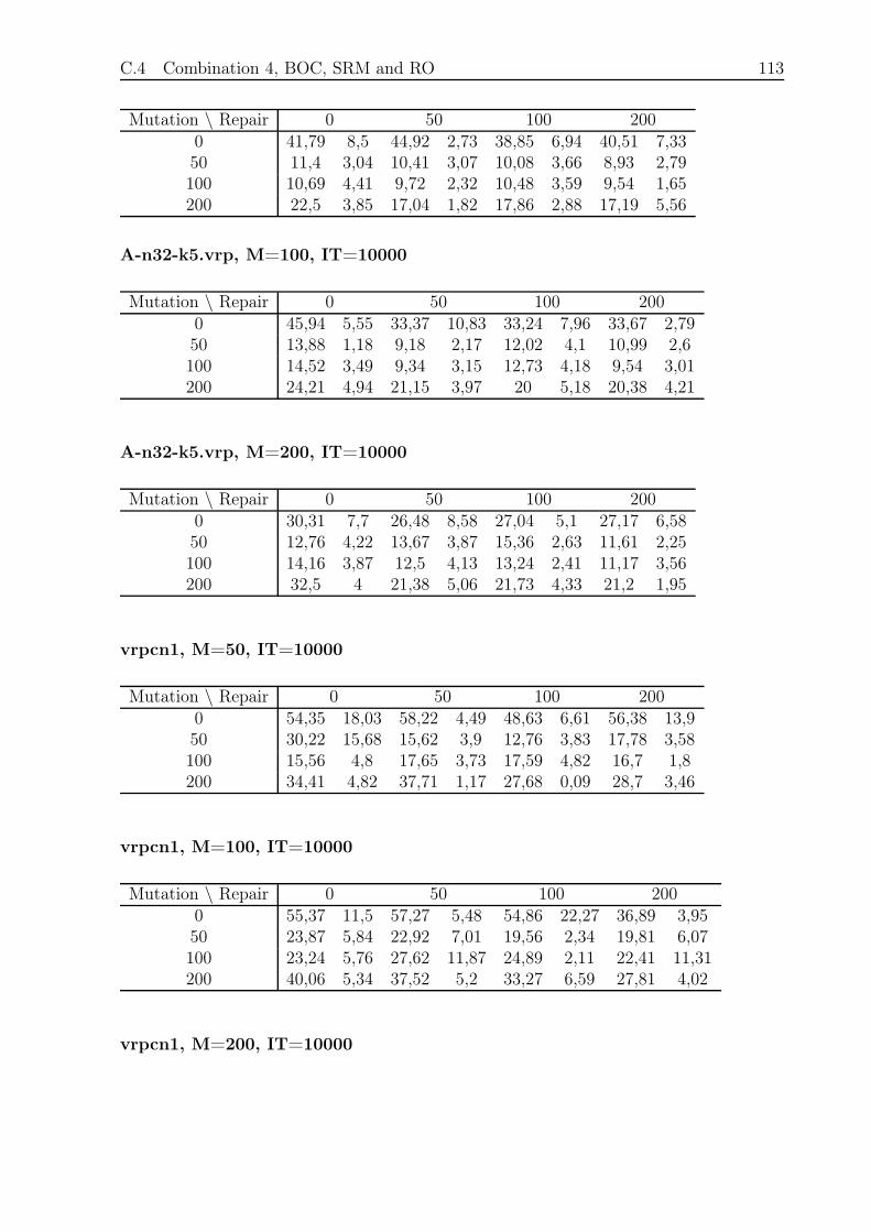
C.4 Combination 4, BOC, SRM and RO 113
Mutation \ Repair 0 50 100 2000 41,79 8,5 44,92 2,73 38,85 6,94 40,51 7,3350 11,4 3,04 10,41 3,07 10,08 3,66 8,93 2,79100 10,69 4,41 9,72 2,32 10,48 3,59 9,54 1,65200 22,5 3,85 17,04 1,82 17,86 2,88 17,19 5,56
A-n32-k5.vrp, M=100, IT=10000
Mutation \ Repair 0 50 100 2000 45,94 5,55 33,37 10,83 33,24 7,96 33,67 2,7950 13,88 1,18 9,18 2,17 12,02 4,1 10,99 2,6100 14,52 3,49 9,34 3,15 12,73 4,18 9,54 3,01200 24,21 4,94 21,15 3,97 20 5,18 20,38 4,21
A-n32-k5.vrp, M=200, IT=10000
Mutation \ Repair 0 50 100 2000 30,31 7,7 26,48 8,58 27,04 5,1 27,17 6,5850 12,76 4,22 13,67 3,87 15,36 2,63 11,61 2,25100 14,16 3,87 12,5 4,13 13,24 2,41 11,17 3,56200 32,5 4 21,38 5,06 21,73 4,33 21,2 1,95
vrpcn1, M=50, IT=10000
Mutation \ Repair 0 50 100 2000 54,35 18,03 58,22 4,49 48,63 6,61 56,38 13,950 30,22 15,68 15,62 3,9 12,76 3,83 17,78 3,58100 15,56 4,8 17,65 3,73 17,59 4,82 16,7 1,8200 34,41 4,82 37,71 1,17 27,68 0,09 28,7 3,46
vrpcn1, M=100, IT=10000
Mutation \ Repair 0 50 100 2000 55,37 11,5 57,27 5,48 54,86 22,27 36,89 3,9550 23,87 5,84 22,92 7,01 19,56 2,34 19,81 6,07100 23,24 5,76 27,62 11,87 24,89 2,11 22,41 11,31200 40,06 5,34 37,52 5,2 33,27 6,59 27,81 4,02
vrpcn1, M=200, IT=10000
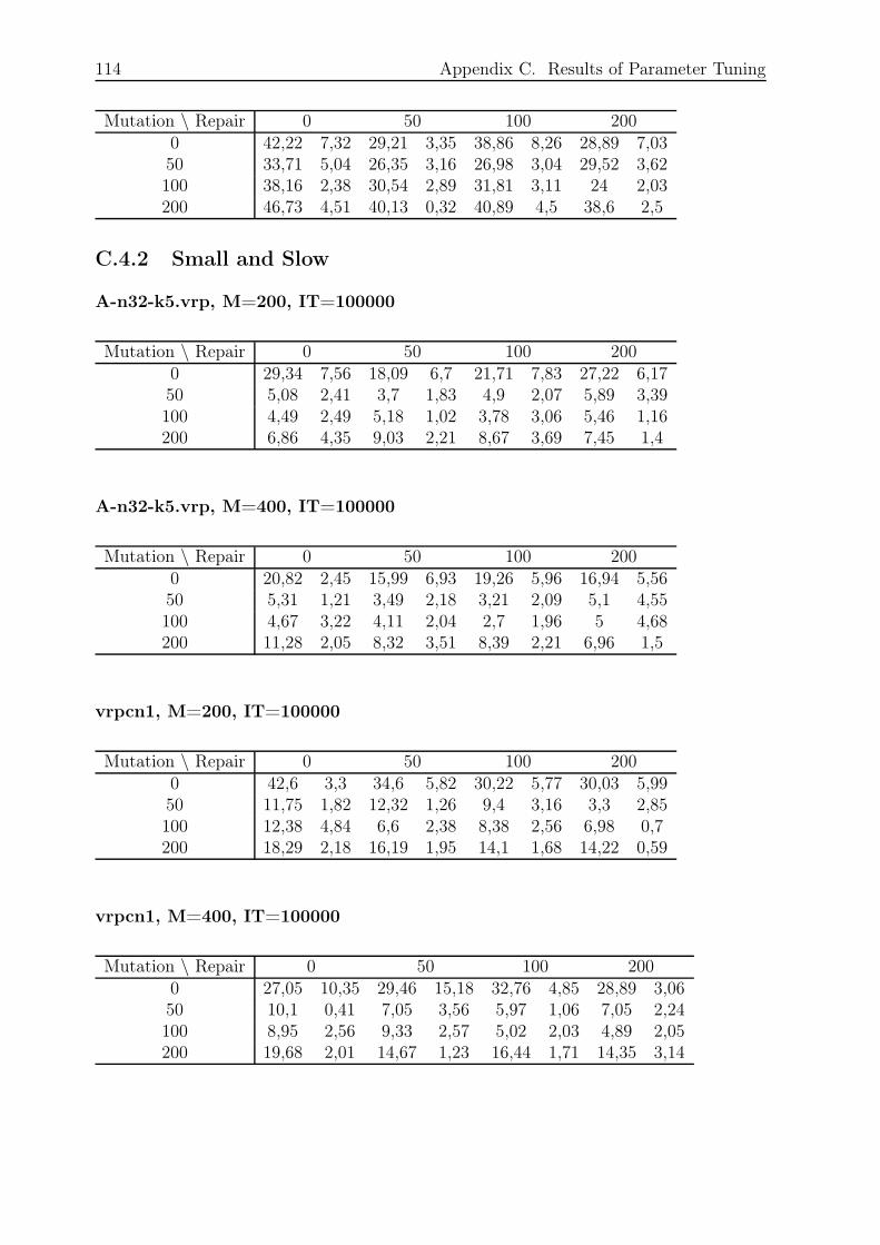
114 Appendix C. Results of Parameter Tuning
Mutation \ Repair 0 50 100 2000 42,22 7,32 29,21 3,35 38,86 8,26 28,89 7,0350 33,71 5,04 26,35 3,16 26,98 3,04 29,52 3,62100 38,16 2,38 30,54 2,89 31,81 3,11 24 2,03200 46,73 4,51 40,13 0,32 40,89 4,5 38,6 2,5
C.4.2 Small and Slow
A-n32-k5.vrp, M=200, IT=100000
Mutation \ Repair 0 50 100 2000 29,34 7,56 18,09 6,7 21,71 7,83 27,22 6,1750 5,08 2,41 3,7 1,83 4,9 2,07 5,89 3,39100 4,49 2,49 5,18 1,02 3,78 3,06 5,46 1,16200 6,86 4,35 9,03 2,21 8,67 3,69 7,45 1,4
A-n32-k5.vrp, M=400, IT=100000
Mutation \ Repair 0 50 100 2000 20,82 2,45 15,99 6,93 19,26 5,96 16,94 5,5650 5,31 1,21 3,49 2,18 3,21 2,09 5,1 4,55100 4,67 3,22 4,11 2,04 2,7 1,96 5 4,68200 11,28 2,05 8,32 3,51 8,39 2,21 6,96 1,5
vrpcn1, M=200, IT=100000
Mutation \ Repair 0 50 100 2000 42,6 3,3 34,6 5,82 30,22 5,77 30,03 5,9950 11,75 1,82 12,32 1,26 9,4 3,16 3,3 2,85100 12,38 4,84 6,6 2,38 8,38 2,56 6,98 0,7200 18,29 2,18 16,19 1,95 14,1 1,68 14,22 0,59
vrpcn1, M=400, IT=100000
Mutation \ Repair 0 50 100 2000 27,05 10,35 29,46 15,18 32,76 4,85 28,89 3,0650 10,1 0,41 7,05 3,56 5,97 1,06 7,05 2,24100 8,95 2,56 9,33 2,57 5,02 2,03 4,89 2,05200 19,68 2,01 14,67 1,23 16,44 1,71 14,35 3,14
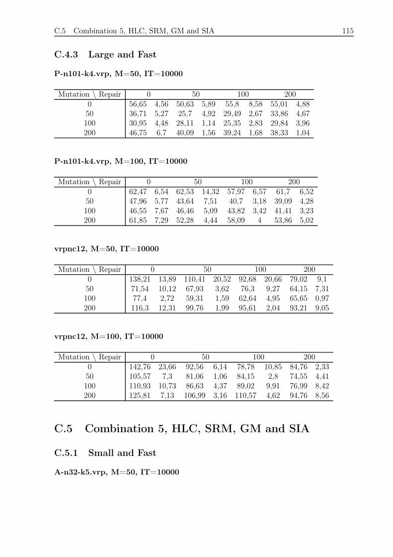
C.5 Combination 5, HLC, SRM, GM and SIA 115
C.4.3 Large and Fast
P-n101-k4.vrp, M=50, IT=10000
Mutation \ Repair 0 50 100 2000 56,65 4,56 50,63 5,89 55,8 8,58 55,01 4,8850 36,71 5,27 25,7 4,92 29,49 2,67 33,86 4,67100 30,95 4,48 28,11 1,14 25,35 2,83 29,84 3,96200 46,75 6,7 40,09 1,56 39,24 1,68 38,33 1,04
P-n101-k4.vrp, M=100, IT=10000
Mutation \ Repair 0 50 100 2000 62,47 6,54 62,53 14,32 57,97 6,57 61,7 6,5250 47,96 5,77 43,64 7,51 40,7 3,18 39,09 4,28100 46,55 7,67 46,46 5,09 43,82 3,42 41,41 3,23200 61,85 7,29 52,28 4,44 58,09 4 53,86 5,02
vrpnc12, M=50, IT=10000
Mutation \ Repair 0 50 100 2000 138,21 13,89 110,41 20,52 92,68 20,66 79,02 9,150 71,54 10,12 67,93 3,62 76,3 9,27 64,15 7,31100 77,4 2,72 59,31 1,59 62,64 4,95 65,65 0,97200 116,3 12,31 99,76 1,99 95,61 2,04 93,21 9,05
vrpnc12, M=100, IT=10000
Mutation \ Repair 0 50 100 2000 142,76 23,66 92,56 6,14 78,78 10,85 84,76 2,3350 105,57 7,3 81,06 1,06 84,15 2,8 74,55 4,41100 110,93 10,73 86,63 4,37 89,02 9,91 76,99 8,42200 125,81 7,13 106,99 3,16 110,57 4,62 94,76 8,56
C.5 Combination 5, HLC, SRM, GM and SIA
C.5.1 Small and Fast
A-n32-k5.vrp, M=50, IT=10000
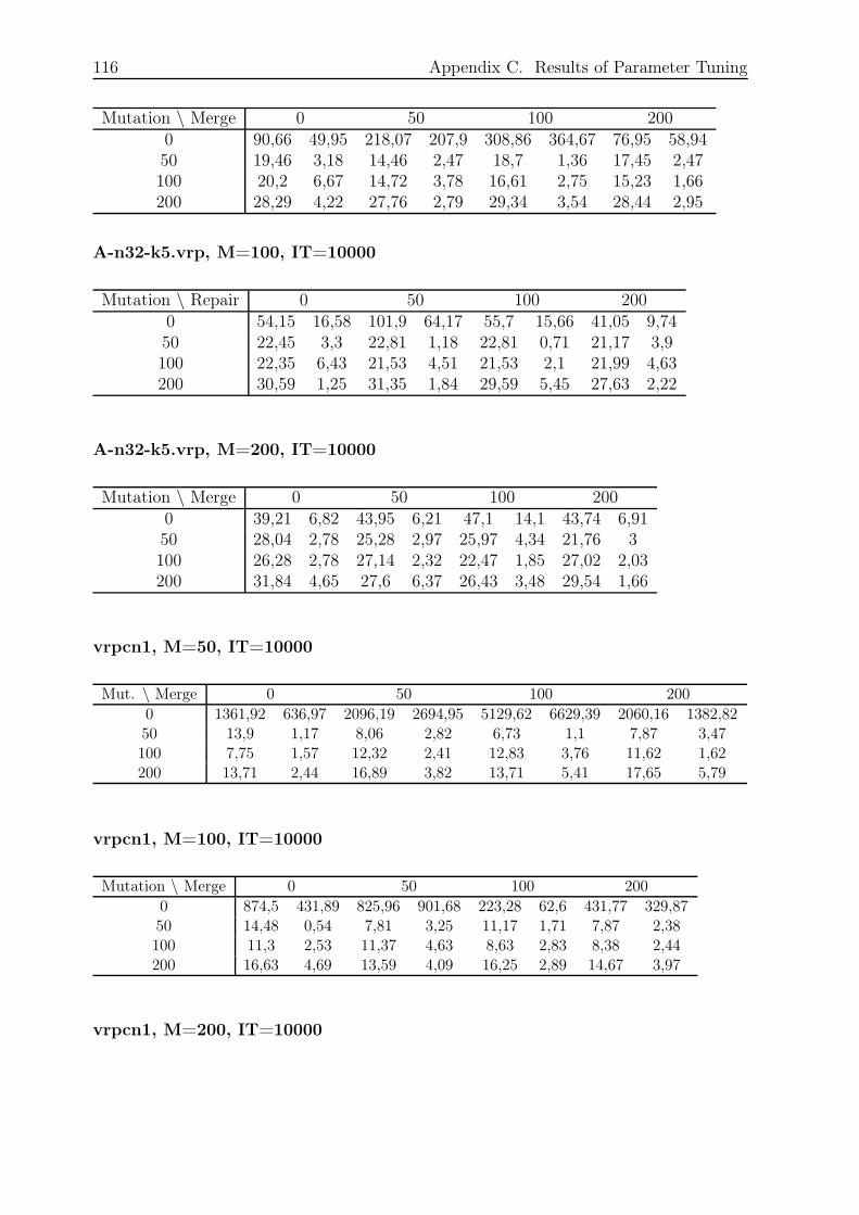
116 Appendix C. Results of Parameter Tuning
Mutation \ Merge 0 50 100 2000 90,66 49,95 218,07 207,9 308,86 364,67 76,95 58,9450 19,46 3,18 14,46 2,47 18,7 1,36 17,45 2,47100 20,2 6,67 14,72 3,78 16,61 2,75 15,23 1,66200 28,29 4,22 27,76 2,79 29,34 3,54 28,44 2,95
A-n32-k5.vrp, M=100, IT=10000
Mutation \ Repair 0 50 100 2000 54,15 16,58 101,9 64,17 55,7 15,66 41,05 9,7450 22,45 3,3 22,81 1,18 22,81 0,71 21,17 3,9100 22,35 6,43 21,53 4,51 21,53 2,1 21,99 4,63200 30,59 1,25 31,35 1,84 29,59 5,45 27,63 2,22
A-n32-k5.vrp, M=200, IT=10000
Mutation \ Merge 0 50 100 2000 39,21 6,82 43,95 6,21 47,1 14,1 43,74 6,9150 28,04 2,78 25,28 2,97 25,97 4,34 21,76 3100 26,28 2,78 27,14 2,32 22,47 1,85 27,02 2,03200 31,84 4,65 27,6 6,37 26,43 3,48 29,54 1,66
vrpcn1, M=50, IT=10000
Mut. \ Merge 0 50 100 200
0 1361,92 636,97 2096,19 2694,95 5129,62 6629,39 2060,16 1382,8250 13,9 1,17 8,06 2,82 6,73 1,1 7,87 3,47100 7,75 1,57 12,32 2,41 12,83 3,76 11,62 1,62200 13,71 2,44 16,89 3,82 13,71 5,41 17,65 5,79
vrpcn1, M=100, IT=10000
Mutation \ Merge 0 50 100 200
0 874,5 431,89 825,96 901,68 223,28 62,6 431,77 329,8750 14,48 0,54 7,81 3,25 11,17 1,71 7,87 2,38100 11,3 2,53 11,37 4,63 8,63 2,83 8,38 2,44200 16,63 4,69 13,59 4,09 16,25 2,89 14,67 3,97
vrpcn1, M=200, IT=10000
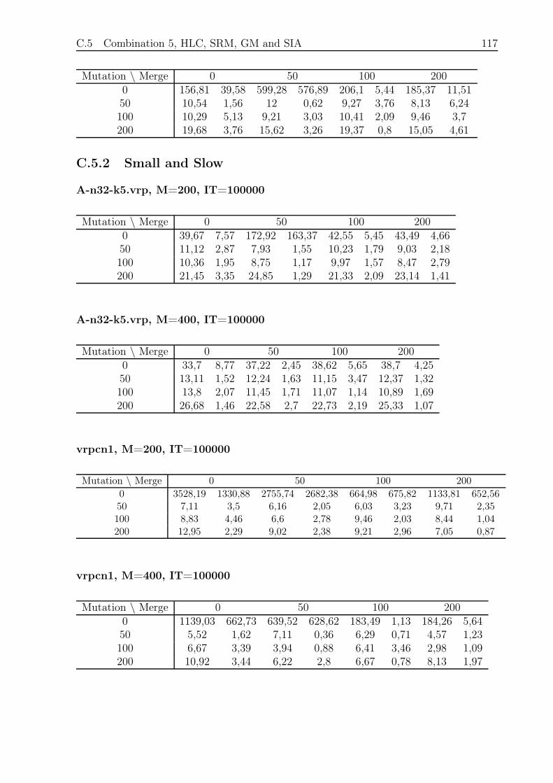
C.5 Combination 5, HLC, SRM, GM and SIA 117
Mutation \ Merge 0 50 100 2000 156,81 39,58 599,28 576,89 206,1 5,44 185,37 11,5150 10,54 1,56 12 0,62 9,27 3,76 8,13 6,24100 10,29 5,13 9,21 3,03 10,41 2,09 9,46 3,7200 19,68 3,76 15,62 3,26 19,37 0,8 15,05 4,61
C.5.2 Small and Slow
A-n32-k5.vrp, M=200, IT=100000
Mutation \ Merge 0 50 100 2000 39,67 7,57 172,92 163,37 42,55 5,45 43,49 4,6650 11,12 2,87 7,93 1,55 10,23 1,79 9,03 2,18100 10,36 1,95 8,75 1,17 9,97 1,57 8,47 2,79200 21,45 3,35 24,85 1,29 21,33 2,09 23,14 1,41
A-n32-k5.vrp, M=400, IT=100000
Mutation \ Merge 0 50 100 2000 33,7 8,77 37,22 2,45 38,62 5,65 38,7 4,2550 13,11 1,52 12,24 1,63 11,15 3,47 12,37 1,32100 13,8 2,07 11,45 1,71 11,07 1,14 10,89 1,69200 26,68 1,46 22,58 2,7 22,73 2,19 25,33 1,07
vrpcn1, M=200, IT=100000
Mutation \ Merge 0 50 100 200
0 3528,19 1330,88 2755,74 2682,38 664,98 675,82 1133,81 652,5650 7,11 3,5 6,16 2,05 6,03 3,23 9,71 2,35100 8,83 4,46 6,6 2,78 9,46 2,03 8,44 1,04200 12,95 2,29 9,02 2,38 9,21 2,96 7,05 0,87
vrpcn1, M=400, IT=100000
Mutation \ Merge 0 50 100 2000 1139,03 662,73 639,52 628,62 183,49 1,13 184,26 5,6450 5,52 1,62 7,11 0,36 6,29 0,71 4,57 1,23100 6,67 3,39 3,94 0,88 6,41 3,46 2,98 1,09200 10,92 3,44 6,22 2,8 6,67 0,78 8,13 1,97
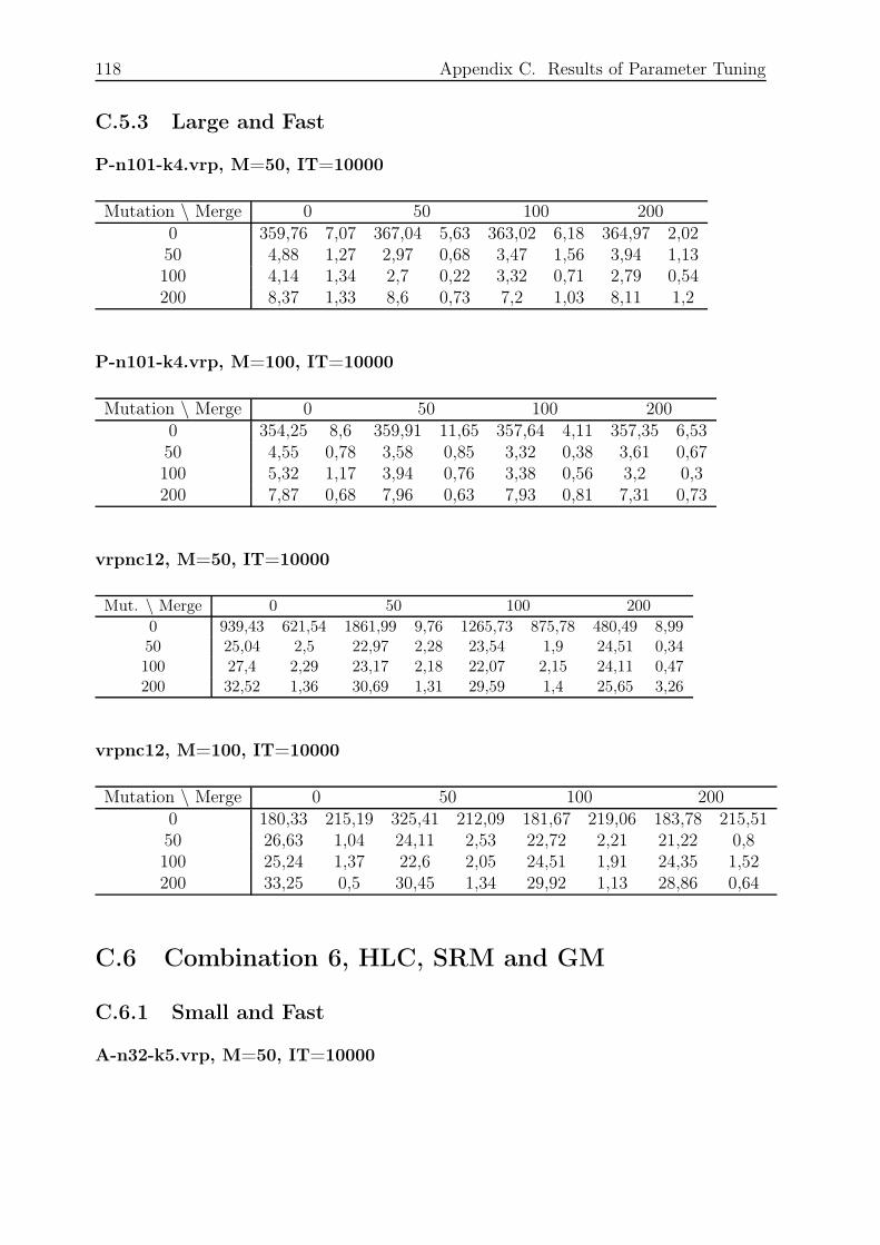
118 Appendix C. Results of Parameter Tuning
C.5.3 Large and Fast
P-n101-k4.vrp, M=50, IT=10000
Mutation \ Merge 0 50 100 2000 359,76 7,07 367,04 5,63 363,02 6,18 364,97 2,0250 4,88 1,27 2,97 0,68 3,47 1,56 3,94 1,13100 4,14 1,34 2,7 0,22 3,32 0,71 2,79 0,54200 8,37 1,33 8,6 0,73 7,2 1,03 8,11 1,2
P-n101-k4.vrp, M=100, IT=10000
Mutation \ Merge 0 50 100 2000 354,25 8,6 359,91 11,65 357,64 4,11 357,35 6,5350 4,55 0,78 3,58 0,85 3,32 0,38 3,61 0,67100 5,32 1,17 3,94 0,76 3,38 0,56 3,2 0,3200 7,87 0,68 7,96 0,63 7,93 0,81 7,31 0,73
vrpnc12, M=50, IT=10000
Mut. \ Merge 0 50 100 200
0 939,43 621,54 1861,99 9,76 1265,73 875,78 480,49 8,9950 25,04 2,5 22,97 2,28 23,54 1,9 24,51 0,34100 27,4 2,29 23,17 2,18 22,07 2,15 24,11 0,47200 32,52 1,36 30,69 1,31 29,59 1,4 25,65 3,26
vrpnc12, M=100, IT=10000
Mutation \ Merge 0 50 100 2000 180,33 215,19 325,41 212,09 181,67 219,06 183,78 215,5150 26,63 1,04 24,11 2,53 22,72 2,21 21,22 0,8100 25,24 1,37 22,6 2,05 24,51 1,91 24,35 1,52200 33,25 0,5 30,45 1,34 29,92 1,13 28,86 0,64
C.6 Combination 6, HLC, SRM and GM
C.6.1 Small and Fast
A-n32-k5.vrp, M=50, IT=10000
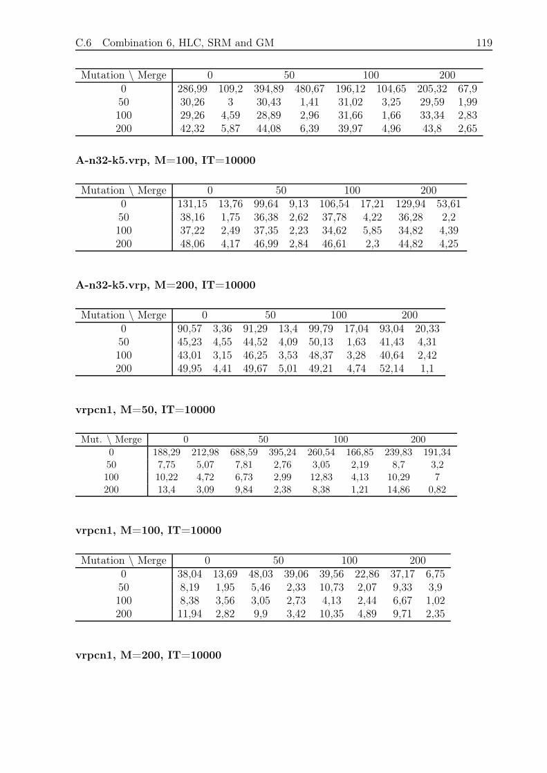
C.6 Combination 6, HLC, SRM and GM 119
Mutation \ Merge 0 50 100 2000 286,99 109,2 394,89 480,67 196,12 104,65 205,32 67,950 30,26 3 30,43 1,41 31,02 3,25 29,59 1,99100 29,26 4,59 28,89 2,96 31,66 1,66 33,34 2,83200 42,32 5,87 44,08 6,39 39,97 4,96 43,8 2,65
A-n32-k5.vrp, M=100, IT=10000
Mutation \ Merge 0 50 100 2000 131,15 13,76 99,64 9,13 106,54 17,21 129,94 53,6150 38,16 1,75 36,38 2,62 37,78 4,22 36,28 2,2100 37,22 2,49 37,35 2,23 34,62 5,85 34,82 4,39200 48,06 4,17 46,99 2,84 46,61 2,3 44,82 4,25
A-n32-k5.vrp, M=200, IT=10000
Mutation \ Merge 0 50 100 2000 90,57 3,36 91,29 13,4 99,79 17,04 93,04 20,3350 45,23 4,55 44,52 4,09 50,13 1,63 41,43 4,31100 43,01 3,15 46,25 3,53 48,37 3,28 40,64 2,42200 49,95 4,41 49,67 5,01 49,21 4,74 52,14 1,1
vrpcn1, M=50, IT=10000
Mut. \ Merge 0 50 100 200
0 188,29 212,98 688,59 395,24 260,54 166,85 239,83 191,3450 7,75 5,07 7,81 2,76 3,05 2,19 8,7 3,2100 10,22 4,72 6,73 2,99 12,83 4,13 10,29 7200 13,4 3,09 9,84 2,38 8,38 1,21 14,86 0,82
vrpcn1, M=100, IT=10000
Mutation \ Merge 0 50 100 2000 38,04 13,69 48,03 39,06 39,56 22,86 37,17 6,7550 8,19 1,95 5,46 2,33 10,73 2,07 9,33 3,9100 8,38 3,56 3,05 2,73 4,13 2,44 6,67 1,02200 11,94 2,82 9,9 3,42 10,35 4,89 9,71 2,35
vrpcn1, M=200, IT=10000
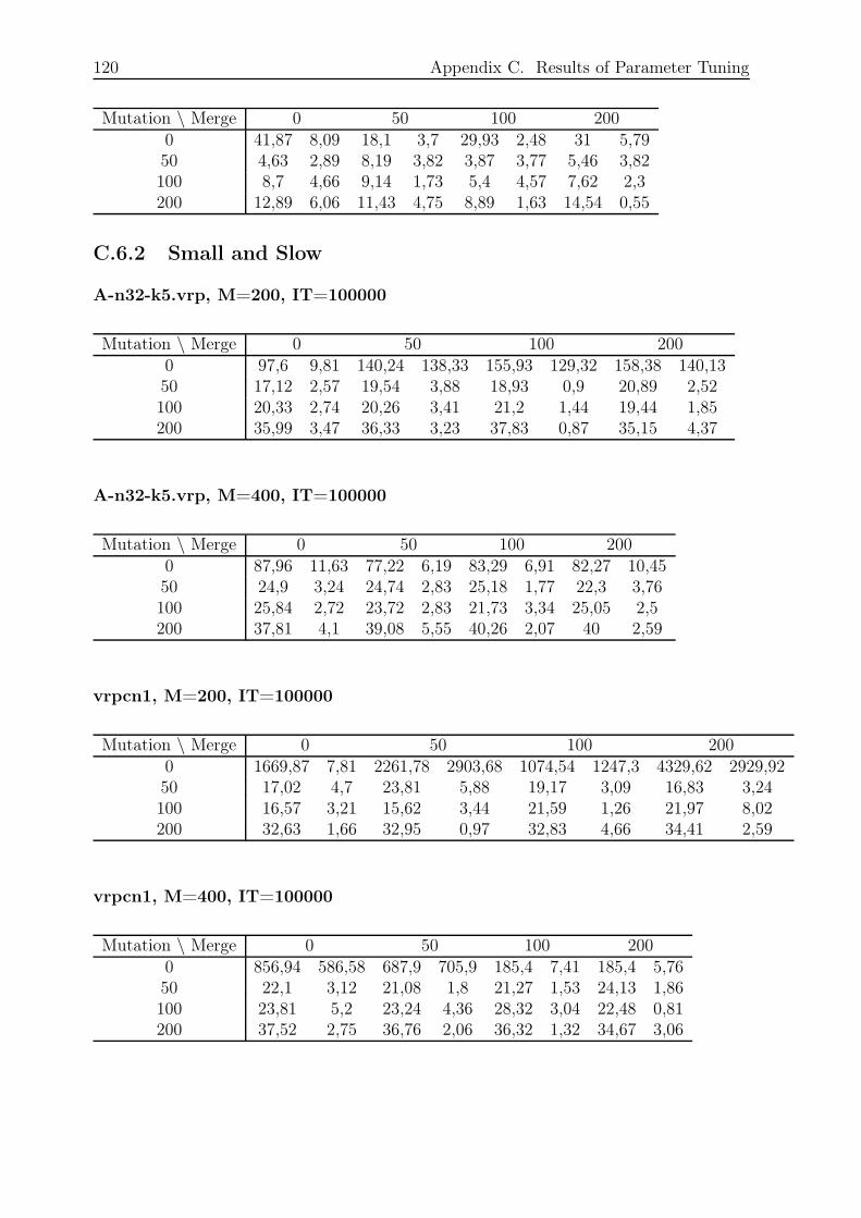
120 Appendix C. Results of Parameter Tuning
Mutation \ Merge 0 50 100 2000 41,87 8,09 18,1 3,7 29,93 2,48 31 5,7950 4,63 2,89 8,19 3,82 3,87 3,77 5,46 3,82100 8,7 4,66 9,14 1,73 5,4 4,57 7,62 2,3200 12,89 6,06 11,43 4,75 8,89 1,63 14,54 0,55
C.6.2 Small and Slow
A-n32-k5.vrp, M=200, IT=100000
Mutation \ Merge 0 50 100 2000 97,6 9,81 140,24 138,33 155,93 129,32 158,38 140,1350 17,12 2,57 19,54 3,88 18,93 0,9 20,89 2,52100 20,33 2,74 20,26 3,41 21,2 1,44 19,44 1,85200 35,99 3,47 36,33 3,23 37,83 0,87 35,15 4,37
A-n32-k5.vrp, M=400, IT=100000
Mutation \ Merge 0 50 100 2000 87,96 11,63 77,22 6,19 83,29 6,91 82,27 10,4550 24,9 3,24 24,74 2,83 25,18 1,77 22,3 3,76100 25,84 2,72 23,72 2,83 21,73 3,34 25,05 2,5200 37,81 4,1 39,08 5,55 40,26 2,07 40 2,59
vrpcn1, M=200, IT=100000
Mutation \ Merge 0 50 100 2000 1669,87 7,81 2261,78 2903,68 1074,54 1247,3 4329,62 2929,9250 17,02 4,7 23,81 5,88 19,17 3,09 16,83 3,24100 16,57 3,21 15,62 3,44 21,59 1,26 21,97 8,02200 32,63 1,66 32,95 0,97 32,83 4,66 34,41 2,59
vrpcn1, M=400, IT=100000
Mutation \ Merge 0 50 100 2000 856,94 586,58 687,9 705,9 185,4 7,41 185,4 5,7650 22,1 3,12 21,08 1,8 21,27 1,53 24,13 1,86100 23,81 5,2 23,24 4,36 28,32 3,04 22,48 0,81200 37,52 2,75 36,76 2,06 36,32 1,32 34,67 3,06
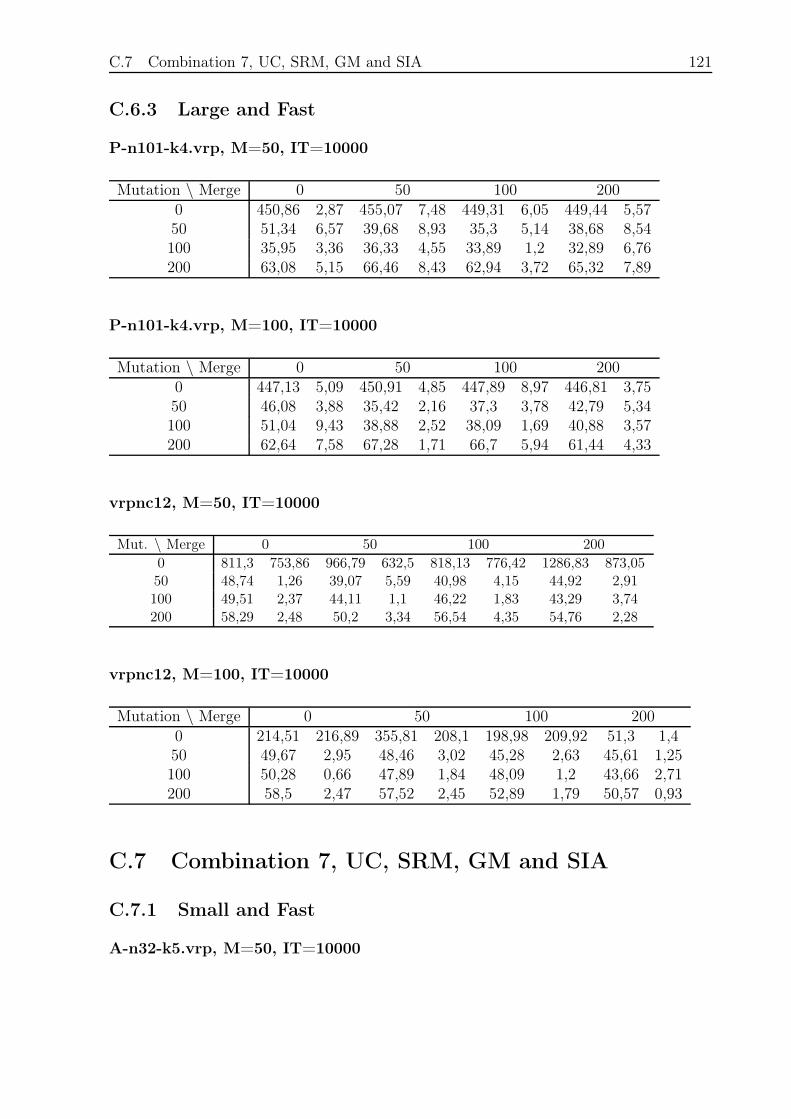
C.7 Combination 7, UC, SRM, GM and SIA 121
C.6.3 Large and Fast
P-n101-k4.vrp, M=50, IT=10000
Mutation \ Merge 0 50 100 2000 450,86 2,87 455,07 7,48 449,31 6,05 449,44 5,5750 51,34 6,57 39,68 8,93 35,3 5,14 38,68 8,54100 35,95 3,36 36,33 4,55 33,89 1,2 32,89 6,76200 63,08 5,15 66,46 8,43 62,94 3,72 65,32 7,89
P-n101-k4.vrp, M=100, IT=10000
Mutation \ Merge 0 50 100 2000 447,13 5,09 450,91 4,85 447,89 8,97 446,81 3,7550 46,08 3,88 35,42 2,16 37,3 3,78 42,79 5,34100 51,04 9,43 38,88 2,52 38,09 1,69 40,88 3,57200 62,64 7,58 67,28 1,71 66,7 5,94 61,44 4,33
vrpnc12, M=50, IT=10000
Mut. \ Merge 0 50 100 200
0 811,3 753,86 966,79 632,5 818,13 776,42 1286,83 873,0550 48,74 1,26 39,07 5,59 40,98 4,15 44,92 2,91100 49,51 2,37 44,11 1,1 46,22 1,83 43,29 3,74200 58,29 2,48 50,2 3,34 56,54 4,35 54,76 2,28
vrpnc12, M=100, IT=10000
Mutation \ Merge 0 50 100 2000 214,51 216,89 355,81 208,1 198,98 209,92 51,3 1,450 49,67 2,95 48,46 3,02 45,28 2,63 45,61 1,25100 50,28 0,66 47,89 1,84 48,09 1,2 43,66 2,71200 58,5 2,47 57,52 2,45 52,89 1,79 50,57 0,93
C.7 Combination 7, UC, SRM, GM and SIA
C.7.1 Small and Fast
A-n32-k5.vrp, M=50, IT=10000
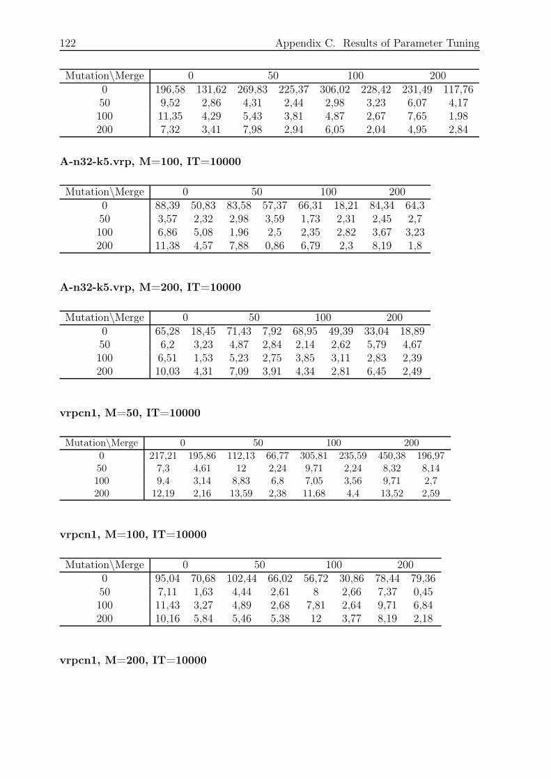
122 Appendix C. Results of Parameter Tuning
Mutation\Merge 0 50 100 2000 196,58 131,62 269,83 225,37 306,02 228,42 231,49 117,7650 9,52 2,86 4,31 2,44 2,98 3,23 6,07 4,17100 11,35 4,29 5,43 3,81 4,87 2,67 7,65 1,98200 7,32 3,41 7,98 2,94 6,05 2,04 4,95 2,84
A-n32-k5.vrp, M=100, IT=10000
Mutation\Merge 0 50 100 2000 88,39 50,83 83,58 57,37 66,31 18,21 84,34 64,350 3,57 2,32 2,98 3,59 1,73 2,31 2,45 2,7100 6,86 5,08 1,96 2,5 2,35 2,82 3,67 3,23200 11,38 4,57 7,88 0,86 6,79 2,3 8,19 1,8
A-n32-k5.vrp, M=200, IT=10000
Mutation\Merge 0 50 100 2000 65,28 18,45 71,43 7,92 68,95 49,39 33,04 18,8950 6,2 3,23 4,87 2,84 2,14 2,62 5,79 4,67100 6,51 1,53 5,23 2,75 3,85 3,11 2,83 2,39200 10,03 4,31 7,09 3,91 4,34 2,81 6,45 2,49
vrpcn1, M=50, IT=10000
Mutation\Merge 0 50 100 200
0 217,21 195,86 112,13 66,77 305,81 235,59 450,38 196,9750 7,3 4,61 12 2,24 9,71 2,24 8,32 8,14100 9,4 3,14 8,83 6,8 7,05 3,56 9,71 2,7200 12,19 2,16 13,59 2,38 11,68 4,4 13,52 2,59
vrpcn1, M=100, IT=10000
Mutation\Merge 0 50 100 2000 95,04 70,68 102,44 66,02 56,72 30,86 78,44 79,3650 7,11 1,63 4,44 2,61 8 2,66 7,37 0,45100 11,43 3,27 4,89 2,68 7,81 2,64 9,71 6,84200 10,16 5,84 5,46 5,38 12 3,77 8,19 2,18
vrpcn1, M=200, IT=10000
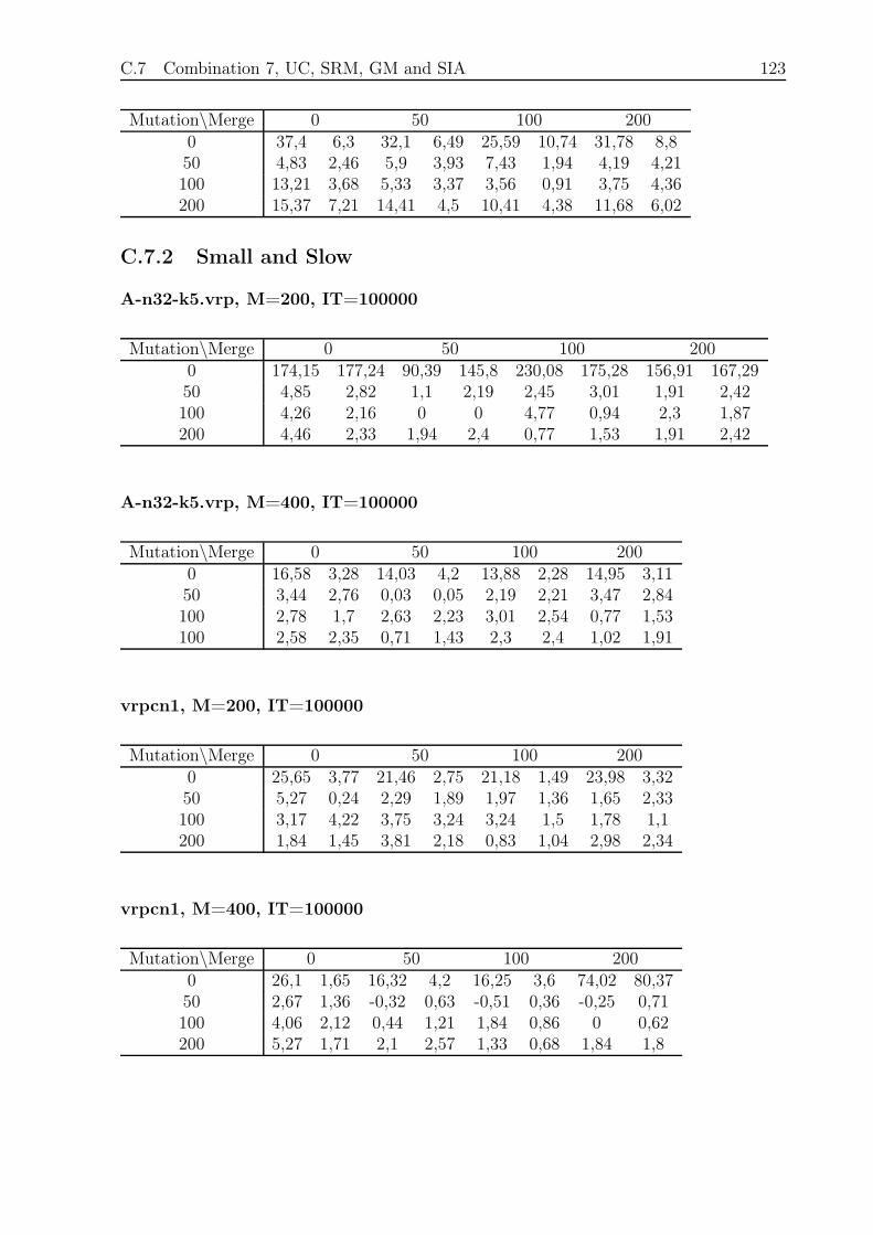
C.7 Combination 7, UC, SRM, GM and SIA 123
Mutation\Merge 0 50 100 2000 37,4 6,3 32,1 6,49 25,59 10,74 31,78 8,850 4,83 2,46 5,9 3,93 7,43 1,94 4,19 4,21100 13,21 3,68 5,33 3,37 3,56 0,91 3,75 4,36200 15,37 7,21 14,41 4,5 10,41 4,38 11,68 6,02
C.7.2 Small and Slow
A-n32-k5.vrp, M=200, IT=100000
Mutation\Merge 0 50 100 2000 174,15 177,24 90,39 145,8 230,08 175,28 156,91 167,2950 4,85 2,82 1,1 2,19 2,45 3,01 1,91 2,42100 4,26 2,16 0 0 4,77 0,94 2,3 1,87200 4,46 2,33 1,94 2,4 0,77 1,53 1,91 2,42
A-n32-k5.vrp, M=400, IT=100000
Mutation\Merge 0 50 100 2000 16,58 3,28 14,03 4,2 13,88 2,28 14,95 3,1150 3,44 2,76 0,03 0,05 2,19 2,21 3,47 2,84100 2,78 1,7 2,63 2,23 3,01 2,54 0,77 1,53100 2,58 2,35 0,71 1,43 2,3 2,4 1,02 1,91
vrpcn1, M=200, IT=100000
Mutation\Merge 0 50 100 2000 25,65 3,77 21,46 2,75 21,18 1,49 23,98 3,3250 5,27 0,24 2,29 1,89 1,97 1,36 1,65 2,33100 3,17 4,22 3,75 3,24 3,24 1,5 1,78 1,1200 1,84 1,45 3,81 2,18 0,83 1,04 2,98 2,34
vrpcn1, M=400, IT=100000
Mutation\Merge 0 50 100 2000 26,1 1,65 16,32 4,2 16,25 3,6 74,02 80,3750 2,67 1,36 -0,32 0,63 -0,51 0,36 -0,25 0,71100 4,06 2,12 0,44 1,21 1,84 0,86 0 0,62200 5,27 1,71 2,1 2,57 1,33 0,68 1,84 1,8
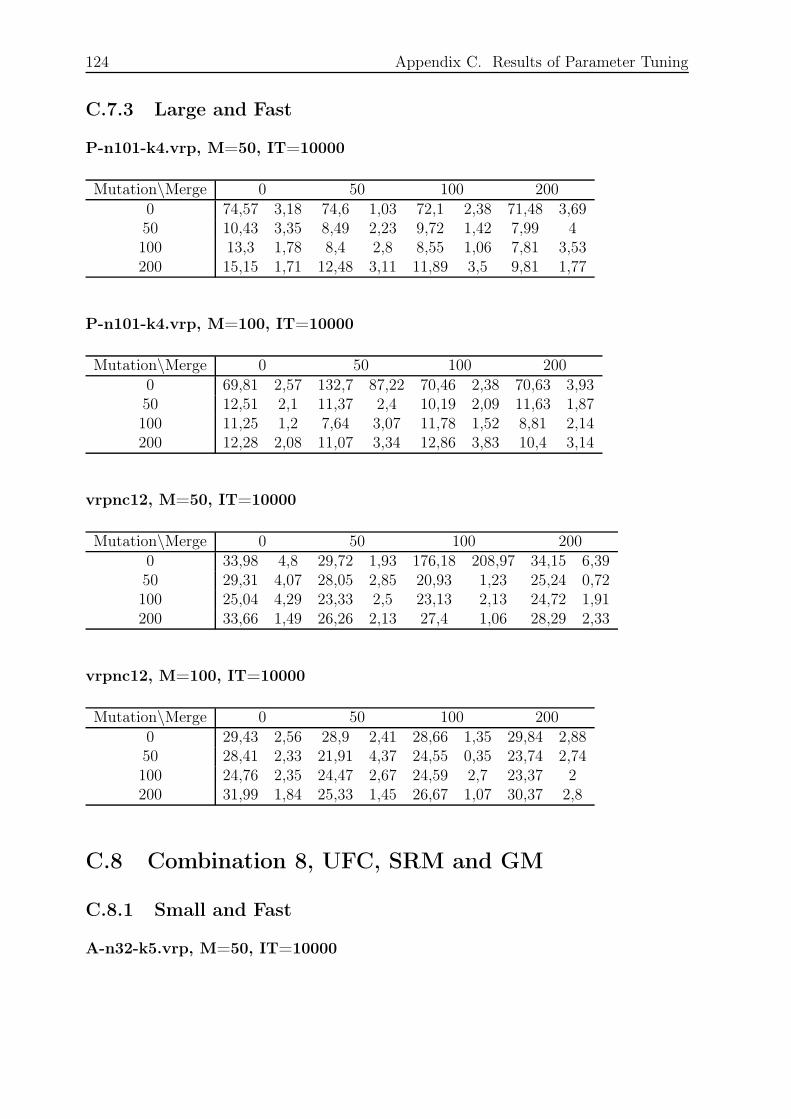
124 Appendix C. Results of Parameter Tuning
C.7.3 Large and Fast
P-n101-k4.vrp, M=50, IT=10000
Mutation\Merge 0 50 100 2000 74,57 3,18 74,6 1,03 72,1 2,38 71,48 3,6950 10,43 3,35 8,49 2,23 9,72 1,42 7,99 4100 13,3 1,78 8,4 2,8 8,55 1,06 7,81 3,53200 15,15 1,71 12,48 3,11 11,89 3,5 9,81 1,77
P-n101-k4.vrp, M=100, IT=10000
Mutation\Merge 0 50 100 2000 69,81 2,57 132,7 87,22 70,46 2,38 70,63 3,9350 12,51 2,1 11,37 2,4 10,19 2,09 11,63 1,87100 11,25 1,2 7,64 3,07 11,78 1,52 8,81 2,14200 12,28 2,08 11,07 3,34 12,86 3,83 10,4 3,14
vrpnc12, M=50, IT=10000
Mutation\Merge 0 50 100 2000 33,98 4,8 29,72 1,93 176,18 208,97 34,15 6,3950 29,31 4,07 28,05 2,85 20,93 1,23 25,24 0,72100 25,04 4,29 23,33 2,5 23,13 2,13 24,72 1,91200 33,66 1,49 26,26 2,13 27,4 1,06 28,29 2,33
vrpnc12, M=100, IT=10000
Mutation\Merge 0 50 100 2000 29,43 2,56 28,9 2,41 28,66 1,35 29,84 2,8850 28,41 2,33 21,91 4,37 24,55 0,35 23,74 2,74100 24,76 2,35 24,47 2,67 24,59 2,7 23,37 2200 31,99 1,84 25,33 1,45 26,67 1,07 30,37 2,8
C.8 Combination 8, UFC, SRM and GM
C.8.1 Small and Fast
A-n32-k5.vrp, M=50, IT=10000
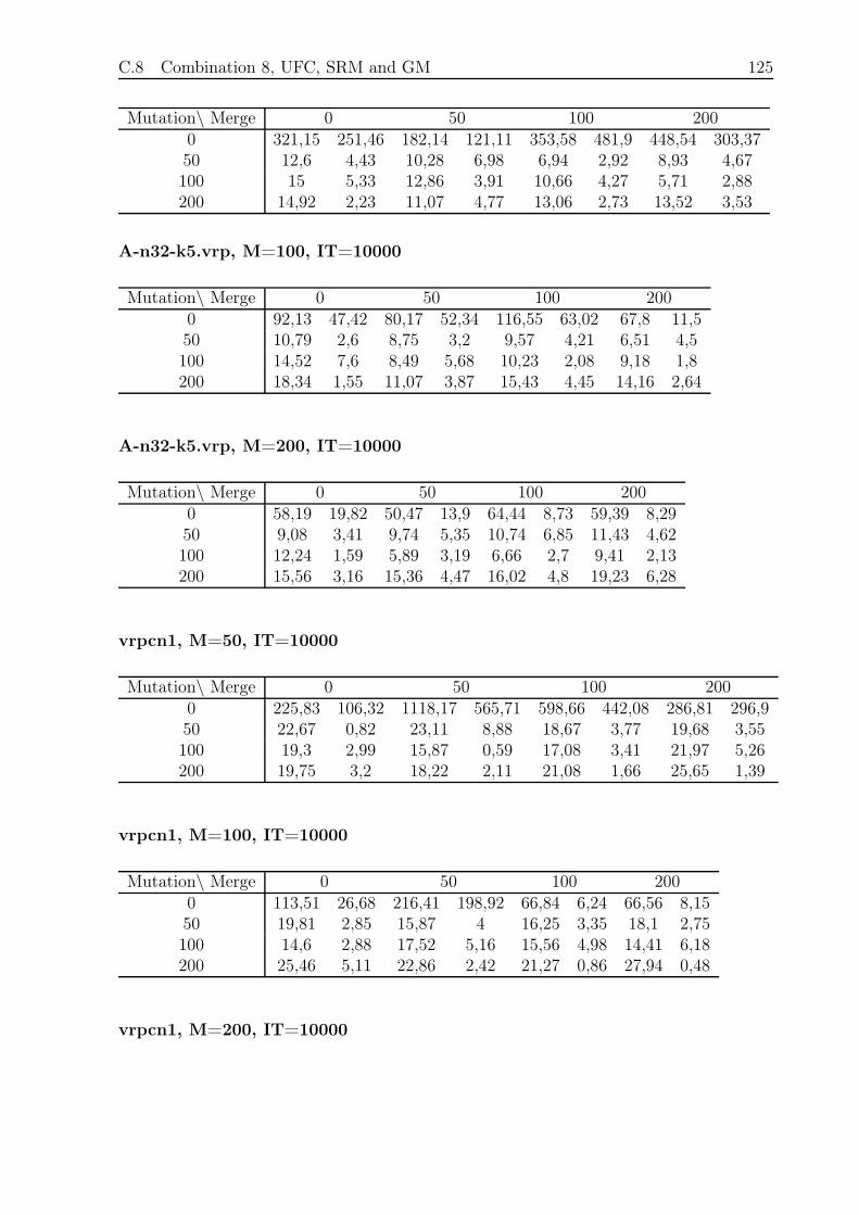
C.8 Combination 8, UFC, SRM and GM 125
Mutation\ Merge 0 50 100 2000 321,15 251,46 182,14 121,11 353,58 481,9 448,54 303,3750 12,6 4,43 10,28 6,98 6,94 2,92 8,93 4,67100 15 5,33 12,86 3,91 10,66 4,27 5,71 2,88200 14,92 2,23 11,07 4,77 13,06 2,73 13,52 3,53
A-n32-k5.vrp, M=100, IT=10000
Mutation\ Merge 0 50 100 2000 92,13 47,42 80,17 52,34 116,55 63,02 67,8 11,550 10,79 2,6 8,75 3,2 9,57 4,21 6,51 4,5100 14,52 7,6 8,49 5,68 10,23 2,08 9,18 1,8200 18,34 1,55 11,07 3,87 15,43 4,45 14,16 2,64
A-n32-k5.vrp, M=200, IT=10000
Mutation\ Merge 0 50 100 2000 58,19 19,82 50,47 13,9 64,44 8,73 59,39 8,2950 9,08 3,41 9,74 5,35 10,74 6,85 11,43 4,62100 12,24 1,59 5,89 3,19 6,66 2,7 9,41 2,13200 15,56 3,16 15,36 4,47 16,02 4,8 19,23 6,28
vrpcn1, M=50, IT=10000
Mutation\ Merge 0 50 100 2000 225,83 106,32 1118,17 565,71 598,66 442,08 286,81 296,950 22,67 0,82 23,11 8,88 18,67 3,77 19,68 3,55100 19,3 2,99 15,87 0,59 17,08 3,41 21,97 5,26200 19,75 3,2 18,22 2,11 21,08 1,66 25,65 1,39
vrpcn1, M=100, IT=10000
Mutation\ Merge 0 50 100 2000 113,51 26,68 216,41 198,92 66,84 6,24 66,56 8,1550 19,81 2,85 15,87 4 16,25 3,35 18,1 2,75100 14,6 2,88 17,52 5,16 15,56 4,98 14,41 6,18200 25,46 5,11 22,86 2,42 21,27 0,86 27,94 0,48
vrpcn1, M=200, IT=10000
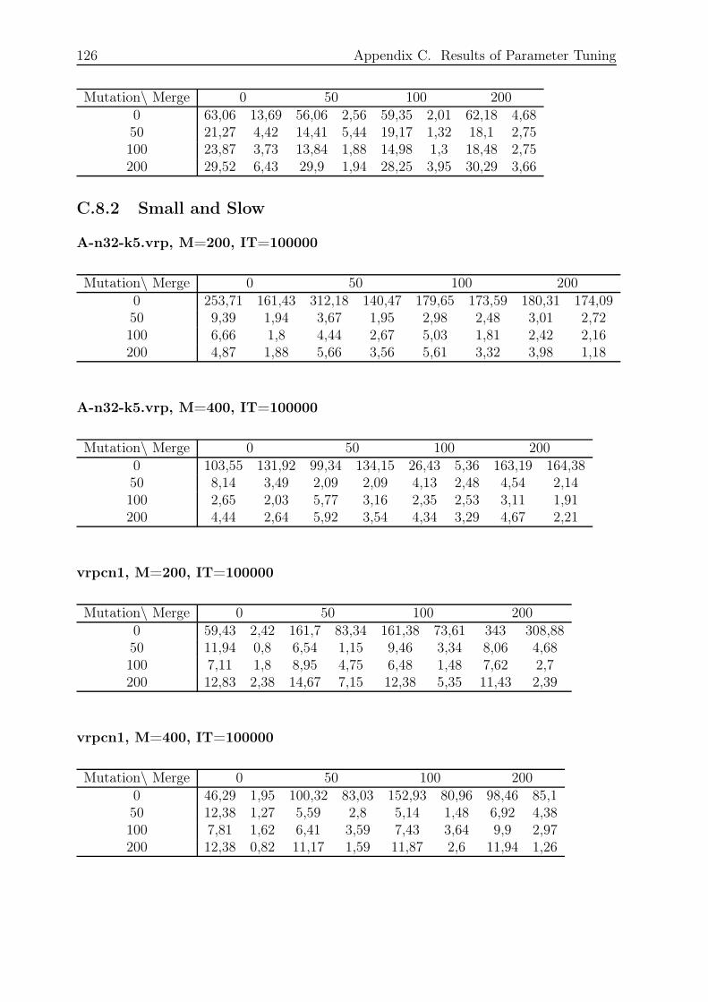
126 Appendix C. Results of Parameter Tuning
Mutation\ Merge 0 50 100 2000 63,06 13,69 56,06 2,56 59,35 2,01 62,18 4,6850 21,27 4,42 14,41 5,44 19,17 1,32 18,1 2,75100 23,87 3,73 13,84 1,88 14,98 1,3 18,48 2,75200 29,52 6,43 29,9 1,94 28,25 3,95 30,29 3,66
C.8.2 Small and Slow
A-n32-k5.vrp, M=200, IT=100000
Mutation\ Merge 0 50 100 2000 253,71 161,43 312,18 140,47 179,65 173,59 180,31 174,0950 9,39 1,94 3,67 1,95 2,98 2,48 3,01 2,72100 6,66 1,8 4,44 2,67 5,03 1,81 2,42 2,16200 4,87 1,88 5,66 3,56 5,61 3,32 3,98 1,18
A-n32-k5.vrp, M=400, IT=100000
Mutation\ Merge 0 50 100 2000 103,55 131,92 99,34 134,15 26,43 5,36 163,19 164,3850 8,14 3,49 2,09 2,09 4,13 2,48 4,54 2,14100 2,65 2,03 5,77 3,16 2,35 2,53 3,11 1,91200 4,44 2,64 5,92 3,54 4,34 3,29 4,67 2,21
vrpcn1, M=200, IT=100000
Mutation\ Merge 0 50 100 2000 59,43 2,42 161,7 83,34 161,38 73,61 343 308,8850 11,94 0,8 6,54 1,15 9,46 3,34 8,06 4,68100 7,11 1,8 8,95 4,75 6,48 1,48 7,62 2,7200 12,83 2,38 14,67 7,15 12,38 5,35 11,43 2,39
vrpcn1, M=400, IT=100000
Mutation\ Merge 0 50 100 2000 46,29 1,95 100,32 83,03 152,93 80,96 98,46 85,150 12,38 1,27 5,59 2,8 5,14 1,48 6,92 4,38100 7,81 1,62 6,41 3,59 7,43 3,64 9,9 2,97200 12,38 0,82 11,17 1,59 11,87 2,6 11,94 1,26
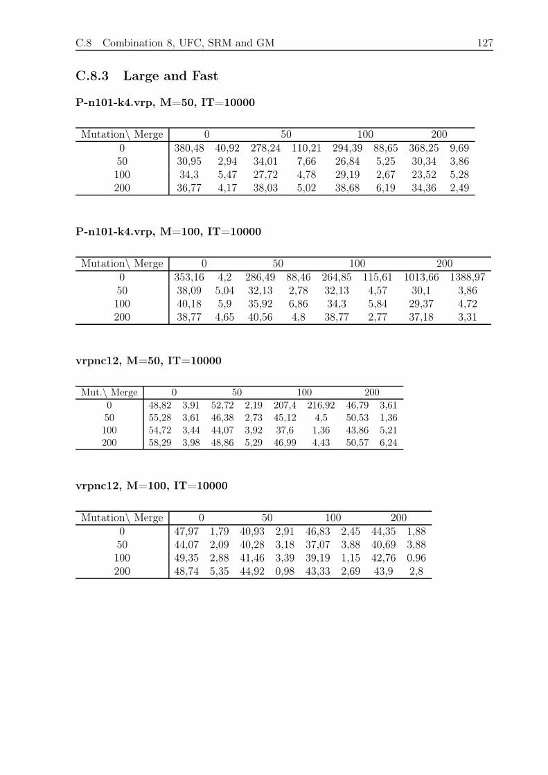
C.8 Combination 8, UFC, SRM and GM 127
C.8.3 Large and Fast
P-n101-k4.vrp, M=50, IT=10000
Mutation\ Merge 0 50 100 2000 380,48 40,92 278,24 110,21 294,39 88,65 368,25 9,6950 30,95 2,94 34,01 7,66 26,84 5,25 30,34 3,86100 34,3 5,47 27,72 4,78 29,19 2,67 23,52 5,28200 36,77 4,17 38,03 5,02 38,68 6,19 34,36 2,49
P-n101-k4.vrp, M=100, IT=10000
Mutation\ Merge 0 50 100 2000 353,16 4,2 286,49 88,46 264,85 115,61 1013,66 1388,9750 38,09 5,04 32,13 2,78 32,13 4,57 30,1 3,86100 40,18 5,9 35,92 6,86 34,3 5,84 29,37 4,72200 38,77 4,65 40,56 4,8 38,77 2,77 37,18 3,31
vrpnc12, M=50, IT=10000
Mut.\ Merge 0 50 100 200
0 48,82 3,91 52,72 2,19 207,4 216,92 46,79 3,6150 55,28 3,61 46,38 2,73 45,12 4,5 50,53 1,36100 54,72 3,44 44,07 3,92 37,6 1,36 43,86 5,21200 58,29 3,98 48,86 5,29 46,99 4,43 50,57 6,24
vrpnc12, M=100, IT=10000
Mutation\ Merge 0 50 100 2000 47,97 1,79 40,93 2,91 46,83 2,45 44,35 1,8850 44,07 2,09 40,28 3,18 37,07 3,88 40,69 3,88100 49,35 2,88 41,46 3,39 39,19 1,15 42,76 0,96200 48,74 5,35 44,92 0,98 43,33 2,69 43,9 2,8