SOME CALCULATIONS ON LEAST-COST DIETSUSING THE SIMPLEX METHOD

By PETER NEWMAN

This paper presents the results of some calculations on the least-costdiet problem, based on the recently invented group of techniques known aslinear programming. Diets for three types of farm animals are presented,and the mixtures of basic feeding stuffs meeting these requirements atminimum cost are calculated. The effects of variations in the prices of feedingstuffs, and of changes in the number of feeding stuffs available are also studied.Certain limitations of the approach are discussed.1

INTRODUCTION

The problem dealt with in this paper is interesting and has considerablepractical importance. Prior to the invention of linear programming, it couldonly be solved by essentially unsystematic hit-or-miss methods. Withproblems involving more than a few variables such tactics prove extremelylaborious, and often practically impossible. We now have available, however,a systematic trial-and-error computing technique that enables exact answersto be given. The computing time is not excessive; an experienced computercan easily perform the full calculations of this model in a day, while the effectof variations in prices and in available feeding stuffs can be handled muchmore quickly.

The rest of this paper is divided into five sections. In the first, I discussthe general problem of least-cost diets. In order to make the treatment self-contained, a brief exposition of the simplex method of linear programming isgiven in the second part. This section may be skipped without loss by thosereaders less interested in technical details. In the third part, the data of thespecific diets are set out, while the results of the computations are presentedand analysed in part four, and certain general problems connected withlinear programming are discussed in the fifth and last section.

PART I. THE PROBLEM

The general problem may be posed quite briefly. It is assumed that inorder to perform certain specified functions (giving two gallons of milk of aspecified fat content per day, laying one egg of specified quality every otherday) an animal requires a daily intake of certain amounts of essential dietaryconstituents such as protein, fibre, phosphorus, etc. These diets are obtainedfrom experiments carried out by dietary experts and are taken as given forthe purposes of the present study.

1 I am indebted to Mr. K. E. Hunt for advice ov- many of the agricultural problemsinvolved, and to Miss Jean Morris, who performed all the considerable computations withgreat skill and efficiency.

304 THE BULLETIN

These dietary constitutents are present in known proportions in all basicfeeding-stuffs, and the appropriate tables are accessible in text books onanimal husbandry. It is assumed that each feeding-stuff is freely available atits market-price, and the problem is to select that mixture of feeding-stuffswhich will satisfy or exceed all the given dietary requirements at least cost.There are an infinite number of mixtures that will do the job, and the problemis to select the cheapest. This is a formidable mathematical problem if thenumber of dietary requirements and feeding stuffs is at all large, and it is onlyrecently that techniques have been developed to solve it.

Some modifications to the problem as it stands should now be made.First, I have assumed that an excess above the given dietary level of some orall constituents is not harmful to the animal concerned. This assumption isprobably correct for the amounts of excess involved in the present investiga-tion. A more exact dietary specification would give upper as well as lowerlimits for the various constituents.'

Secondly, the average farmer, at least in Britain, does not rely only onpurchased feeding-stuffs, but has available home-grown feeds, such aspasture, roots and hay, all of which contain the essential dietary constituents.In a sense, his problem is more difficult, for he has to blend bought feeding-stuffs with his own produce to arrive at an optimal diet. Ideally, he shouldcost his own produce at some appropriate price, but this is seldom done.It is probably better, therefore, to approach the problem from the viewpointof a manufacturer of blended feeding-stuffs. I shall assume that he wishesto market a compounded feeding-stuff that will satisfy or exceed certaindietary requirements. He is naturally and properly interested in doing thisin the most efficient manner, i.e. at least cost. It will further be assumed thatthe compound is marketed in ioo lb. sacks, and that he therefore wishes toproduce the cheapest possible mixture weighing xoo lb. and meeting thespecifications. The use of ioo lb. is merely for ease of computation; problemsinvolving alternative weights, e.g. I 12 lb., could easily be computed.

A final qualification belongs as much in the section on results as it doeshere. Although not conversant with agricultural methods, nor even withagricultural economics, I have made considerable efforts to obtain realisticdata. Nevertheless, some readers, especially those with agricultural experi-ence, may feel that some of the results are unacceptable on a priori grounds.This divergence can be explained in at least three ways. First, and probablyof least importance, is the possibility that these readers may be wrong; thatthis exact analysis shows up errors that have long persisted in the industry.For example, one of the similar investigations carried out in the United States2

1 A similar problem was of crucial importance in the linear prograniniing analysis of theblending of certain aviation petrols. See A. Chames, W. W. Cooper and B. Mellon: Blend-ing Aviation GasolinesA Study in Programming Interdependent Activities in an Inte-grated Oil Company': Economefrica, Vol. 20, No. 2, April 1952, pp. 135-59.

2 F. V. Waugh: The Minimum Cost Dairy Feed': Journal of Farm Economics,Vol. 33, No. 3, August 1951, pp. 299-310; and W. D. Fisher and L. W. Schreiben: 'LinearProgramming Applied to Feed-Mixing under Diflerent Price Conditions ', Journal of FarmEconomics, Vol. 35, No. 4, November 1953, pp. 471-83.

CALCULATIONS ON LEAST-COST DIETS 305

indicated that oilcakes were considerably over-priced. A second possibilityis that the data are themselves in error, so that any conclusions resulting fromoperations on them are also in error. A final reason for this divergence mightbe errors or omissions in the dietary specifications. It might be, for example,that the combination of foods in an optimum diet is altogether unpalatable,1e.g. in a similar problem for human beings, the optimum mixture mightconsist of pickled onions, yoghourt, and chocolate nut sundaes with whippedcream and hot fudge sauceperhaps enjoyable for a change, but not as asteady diet. This points to an incomplete specification, since one should knowwhat diets are excluded on such grounds. In this study we deal with thisproblem partially by completely excluding these foods which in toto aredistasteful or harmful to a particular animal e.g. fish meal when fed to cowshas bad effects on the quality of the milk. The problem of unpalatableproportion.s remains.

One result, obtainable directly from the use of the simplex method, may bestated here in anticipation of the detailed results given in Part IV. A mathe-matically trivial (but not intuitively obvious) result of casting the probleminto linear programming form2 is that the cheapest diet will contain no morebasic feeding stuffs than there are constraints on the solution; it may containless. Thus in the first diet giveQ in Part III, where the only limitationsare on starch equivalent, protein equivalent, and total weight of the mixture,the optimum mixture will contain not more than three feeding stuffs. Inthe poultry problem, where there are two additional constraints, the solut!onsatisfying the conditions laid down will consist of not more than five feedingstuffs. The next Part deals briefly with the mathematical and more explicitlywith the computational aspects of the simplex method, and may be omittedwithout serious loss of continuity.

PART II. THE METHOD

In this Part, a brief resumé of the simplex method, which is due to Dantzig3is given, stress being laid on its computational aspects.4

The problem may be stated concisely thus:Let x1, x2, . . . , x,, be a finite set of variables, and let Pi' P2, . . . p be a corres-ponding set of non-negative numbers (prices). Most economic problems aresuch that solutions containing negative numbers are nonsensical. Thereforewe impose the restrictions

x1>0,x2>0, xn>o (i)I owe this point to Dr S. Vajda.

3 See G. B. Dantzig: Maximisation of a Linear Function of Variables subject to LinearInequalities,' which is Chapter XXI of Activity Analysis of Production and Allocation,edited by T. C. Koopxnans. Cowles Commission Monograph No. 13, Wiley, 1951.

' Loe. cit.Readers wanting a fuller account are referred to Koopmans, op. cit., Chapters XXI and

XXII; to A. Chames: 'Optimality and Degeneracy in Linear Programming,' Econom-etrica, Vol. 20, No. 2, April 1952, pp. 160-70; and to A. Chames, W. W. Cooper and A. M.Henderson: An Introduction to Linear Programming, Wiley, New York, 1953. A forth-coming book by Dr. S. Vajda may also profitably be consulted.

Figure la. Figure lb.1 Simple examples along these lines are discussed more fully in Chapter 14 of J. C. C.

McKinsey: Introduction to the Theory of Games, published for the RAND Corporation by[Footnote continued on following page

306 THE BULLETIN

In addition to these inequalities, certain other inequalities are imposed.Thus the lower limit for the starch equivalent in diet (a) given in Part IIImay be expressed as follows:

a11 X1 + a12 X2 + a1 19 19 > 71.4where the a1 denotes the proportions of starch equivalent in feeding stuff j,e.g. putting x1 linseed, a11 becomes .740. The weight limitation may bewritten as

X1 + X2 + + X19 100The problem of linear programming, then is to minimise (or maximise)

the linear functionalZ = Pi X1 + P2 x2 + + px (z)

subject to the m linear inequalitiesa11x1 + a12x2 + + a10x0>b1a21X1 + a22x2 + + a2x>b2

(3)

ami xi + ax2 + + 1mfl Xn> bmand the restrictions (i), repeated below

X1>0,X2>0, Xn>0 (i)The problem is now stated; the difficulty is to solve it. First, in order to

get some idea of the geometry of the problem, let us consider a very simpleexample1 illustrated in Figures r and 2. Suppose that there are only twovariables x1, and x2, and only two constraints, represented by the inequalities

a11 x1 + a12 x2 > b1 (4)a21 x + a22 X2 > b2

These are drawn in Figure (a) and (b) respectively.

CALCULATIONS ON LEAST-COST DIETS 307

All points lying along the line given by the equationa11 x1 + a12 x2 = b1

are such that the first constraint is just satisfied; similarly for the secondconstraint. Ail points to the right of the line more than satisfy the particularlimitation.

Now let us superimpose the two constraints on the same diagram, as inFigure 2. It is convenient to treat two cases, one derived from Figure x, andanother invented for the purpose. In the first case, represented in Figure za,the superposition of the two constraints divides the quadrant of non-negativex1 and x2 into four disjoint regions, labelled (a), (b), (c) and (d). None of the

C

X2-. L)

Figure 2a. Figure 2b.points in (a) satisfy either of the two constraints; those in (b) satisfy the firstconstraint but not the second, while those in (c) satisfy constraint z but notconstraint i. Only those points in (d) satisfy, or more than satisfy, bothlimitations taken together. The problem, it will be remembered, is to findthat combination of x1 and x2 which satisfy the limitations at least cost. Itis intuitively clear that this optimum combination will occur on the boundaryof region (d).

Figure zb illustrates the case where one of the constraints is the dominantone, completely determining what the optimum combination will be. Thepositive quadrant is now split into three regions; one where neither constraintis fulfilled, one where the second but not the first is fulfilled, and the lastwhere both constraints are satisfied. Constraint 2 is ineffective, for if constrainti is satisfied, this automatically guarantees the fulfillment of constraint z.We shall ignore such constraints in the ensuing development of the theory,though they are common enough in practice.McGraw Hill, New York, 1952; and in G. Morton: 'Notes on Linear Programming'Economica, N.S. Vol. XVIII, November 1951, pp. 397-411. The best discussions of therelation of this approach to the usual techniques of economic theory are contained in R.Dorf man: ApplIcation of Linear programming to the Theory of the Firm, University of Cali-fornia, 1951; and Dorfman 'Mathematical, or "Linear" Programming: A Non-mathematical Exposition, American Economic Review, Vol. XLIII, No. 5, December 1953,pp. 797-825.

308 THE BULLETIN

We shall now demonstrate the solution to the least-cost problem in thistwo-commodity, two-constraint case. The total cost of the two commoditiesis given by z, where

z=p1x1+p2x2 ()and Pi' P2 are the prices of x1 and x2 respectively. This cost function canitself be represented as a straight line in a diagram similar to Figure za, with

slope -e-'. The problem is to minimise z. Now we may imagine a line withP2

slope moving outwards from the origin until it first touches the boundaryP2

of (d), the area which satisfies both inequalities of (.).This process is illustrated in Figure 3.

Figure 3.If the kink at Q is well marked, it is highly probable that the solution is

provided by the combination represented by Q. If the price line has a slopeless than the slope of constraint i, however, the solution is found by using x1exclusively; and correspondingly for constraint z and x2. There are twoborderline cases where the relative prices coincide with either the slope ofthe first constraint, or the slope of the second. In these cases, equilibrium isindeterminate, the equilibrium combination being any point on the appro-priate part of the boundary.

It will be noticed that in the common case, where equilibrium is at Q,quite wide swings in relative prices will fail to result in a different optimumcombination. This is a phenomenon that will occur frequently in the empiricalresults.

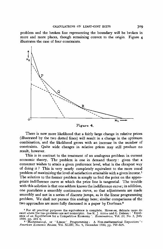
More and more constraints may be introduced into the two-commodity

CALCULATIONS ON LEAST-COST DIETS 309

problem and the broken line representing the boundary will be broken inmore and more places, though remaining convex to the origin. Figure 4illustrates the case of four constraints.

Figure 4.

There is now more likelihood that a fairly large change in relative prices(illustrated by the two dotted lines) will result in a change in the optimumcombination, and the likelihood grows with an increase in the number ofconstraints. Quite wide changes in relative prices may still produce noresult, however.

This is in contrast to the treatment of an analogous problem in currenteconomic theory. The problem is one in demand theory: given that aconsumer wishes to attain a given preference level, what is the cheapest wayof doing it ? This is very nearly completely equivalent to the more usualproblem of maximisirig the level of satisfaction attainable with a given income.'The solution to the former problem is simply to find the point on the appro-priate indifference curve at which the price line is tangential. The troublewith this solution is that one seldom knows the indifference curve; in addition,one postulates a smoothly continuous curve, so that adjustments are madesmoothly and not in a series of discrete jumps, as in the linear programmingproblem. We shall not pursue this analogy here; similar comparisons of thetwo approaches are more fully discussed in a paper by Dorfman.2

For all practical purposes the equivalence is complete. However, delicate cases doexist where the two problems are not isomorphic. SeeK. J. Arrow and G. Debreu: 'Exist-ence of an Equilibrium for a Competitive Economy'. Econometrica, Vol. 22, No. 3, July1954, pp. 285-6.

2 'Mathematical, or 'Linear' Programming: A Non-mathematical Expositiøn':American Economic Review, Vol. XLIII, No. 5, December 1953, pp. 797-825.

310 THE BULLETIN

It is now perhaps easier to visualise the situation when there are n com-modities. The boundary of the set of x's which satisfy the constraints willnow look like the surface of an n-dimensional crystal, with innumerablefacets. The linear functional which we are trying to minimize will now bean n-dimensional hyperplane which can be imagined to be advancing steadilyfrom the origin of the n-dimensional space towards the crystal, which issuspended in the positive octant of the space. The problem is to determinethe point or points (in n-space) at which the hyperplane will hit the crystal.The way in which we solve it is to land on the crystal and crawl over it insome systematic way, from extreme point to extreme point, until we find oneor more which we know to be correct. This is not quite the whole story, ofcourse, for one may quite easily pose problems to which no solution exists.However, the crude geometrical picture that has been drawn contains thegist of the matter. The simplex method provides a systematic way of crawlingover the surface of the crystal. Further, it has several important properties. Ifone were to explore the crystal in an unsystematic way there is no guaranteethat one would not double back on one's tracks and so on ad infinitum. Itwould be nice to know, also, that at each step things got better and better,bringing one nearer the goal, or at least no further away from it. The simplexmethod does just this. At each stage one approaches nearer the solution, andat each stage, by a suitable check, one can tell (a) whether a solution exists,(b) whether one has attained the solution and (c) whether further computa-tions are required. We now proceed to a description of the computationaldetails.

The first step in the simplex method is to convert the inequalities (3) intoequalities. This is achieved by bringing in so-called 'pseudovariables ',one for each inequality, which ' take up the slack' of the inequalities. Thus,if the lower limits are exactly met, the pseudovariable takes the value o.In this way the set () becomes:

a11 X1 + a12 X2 + . .. + a1, x + x,,1 + o +.. . + o = b1a21x1 +a22x2 + . . . + + o + x,2+ .. +o = b2

()

a X1 + am2 X2 +... + amn X + O + O + ... + Xn+m = bmThe pseudo-variables have a zero price, so that their presence in the final

solution will add nothing to its cost. One difficulty that occurs in our problemis that one of the limitations, that on weight, is a strict equality. In order toachieve this, we adopt the following device (remembering, as Richard Bellmanhas pointed out, that a device is a trick that works at least twice). To thepseudo-variable occurring in the equation for the weight limitation, we attacha large positive price M, where M need not be explicit, but is taken as manytimes larger than any other price. No solution which contains this enormous

'See A. Chames: 'Optimality and Degeneracy in Linear Programming,' Econometyica,Vol. 20, No. 2, April 1952, pp. 160-70.

CALCULATIONS ON LEAST-COST DiETS 311

price M will be a minimizing solution, so the value of the correspondingpseudo-variable will be zero. This procedure' works for any number ofequalities that we may wish to make out of the inequalities (3).

It is convenient to regard the set of numbers a11, a21, a31, . . . a as asingle point A, of rn-dimensional Euclidean space, and the column b1, b,,

bm as another point, say A0, in the same space. The linear programmingproblem then becomes:

Find x1, X,, . . . x, x,1, . . .

such thatx1 A1 + x2 A2 +... + x0 A +... + XU+m An+m = A0 (6)

andX, p, + X, P, +... + x0 p, = z = minimum (7)(The problem of maximising z may be treated symmetrically by minimu.-

ing -z).The next step is to guess at a solution, that is, to select a set of m A's

which, multiplied by positive x's will satisfy (6). More succinctly, choose mA1's such that

A1 + 2 A, +... + m Am = A0 with £ > o. (8)Without loss of generality, we may take the first m of the A's to be such abasis as it is called. This basis consists, in our problem, of a set of feedingstuffs which can be combined in irt least one way to satisfy the dietary restric-tions. They need not, and normally will not, constitute the cheapest diet, butthey do provide what is known as a feasible solution. In small problems suchas ours a feasible solution can usually be arrived at very easily, and an inspiredguess, which may very well come from those familiar with a given economicproblem, may do wonders in shortening the computing time involved. Inlarger problems a feasible solution is usually not so obvious. However,methods exist for computing a feasible solution,2 and recent modifications ofthe simplex method3 do not in fact require one to start from a feasible solution.

We now try to proceed from a basic feasible solution to an optimum basicfeasible solution. To do this, we first express all other vectors Am+i, Am+2,

Am+n, A0 in terms of the basis vectors A1, A,, . . . Am, e.g.x1 A1 + x, A, + ... + Xmj A = A (9)

There are two important special cases of (o). One is simplyIA1+OA2+...+OAm=Pi (io)

and so on for all A in the basis, and the other isXi3O A, + x,,0 A, + . + Xm, o Am = A0 (ii)

i.e. the requirements are expressed in terms of the basis vectors. These

'See A. Chames, W. W. Cooper and A. M. Henderson: An Introduction to Linear Pro-grarnming, Wiley, New York, 1953.

Koopmans (cd.) op. cit., Chapter 21.Chames, op. cit.; G. B. Dantzig and Others: 'Notes on Linear Programming,' Rand

Reports, P- 392, 393, 394, 440, 460, 472, October 1953January 1954; E. M. L. Beale:'An Alternative Method of Linear Programming,' P'oceedings oft/ic Cambridge PhilosophicalSociety, Vol. 50, October 1954, pp. 513-523; C. E. Lemke: 'The Dual Method of LinearProgramming, Technical Report No. 29 of the Department of Mathematics, CarnegieInstitute of Technology, Pittsburgh, Pennsylvania, March 1953.

3X2 THE BULLETIN

X, X20, . . . correspond to the i, X of (8), and constitute thelevels of the variables whose vectors constitute the basis.

The calculations are best set out in the form of a 'simplex tableau

We set this out for m = 4 and n = 5. It should be noticed that there is noreason why the original basis should not contain some pseudo-variables.In fact it often simplifies the task of obtaining an initial feasible solution.Having set out all the vectors in terms of linear combinations of the basicvectors,2 we then compute certain sums. The initial value z0 of the linearfunctional z is given by

pl i + PX2 ± P33 + 4X4 z0The value of, say, z5 is given by

p1 x15 + p2x25 + p3x + p4x4 = z5 (13)For A1, A2, A3 and A4 the corresponding z's are simply the prices p1, p2, p3,and p4, and their entries on the lowest line are zero. For the others wecompute z5 - p5 and note whether the result is positive or negative. If allthe z5 - p are negative then the basic theorems of the simplex method tellus that the minimum has been attained and that z0 is

t.3Another case occurs

if all the are negative: in this case no minimum exists. The common case,however, is that some of the z5 - p5 will be positive. Then the simplexmethod tells us that one can lower z0 further by removing one of the basisvectors and substituting another vector not already in the basis.

We now need criteria to tell us which vector to throw out of the basis,and which to put in. Any vector giving a positive z5 - p5 is eligible to beput into the basis, but empirically it appears that the best results are obtainedwhen that vector, say A6, giving the largest value of z5 - p5 is put in. Inorder to determine the vector to throw out, we consider the column vector A6,compare the ratios 1/x16, 2/x26, 3/x36 and 4/x36, and select that basis vector,say A4, which gives the largest algebraic value of the ratio. A3 is then thrownout, and all the column vectors are recomputed using the new basis A1, A2,A4 and A6. It is a theorem of Dantzig's4 that this new basis must resultin a decrease of z0, and so is a step nearer the optimal mixture.

'Chames, op. cit., p. 165.As in Chames, op. cit.Appropriate adjustments have to be made here and throughout the analysis if one is

maximizing a linear functional rather than minimizing it. See Koopmans (ed.), op. cit.Chapter XXI.

'Koopinans (ed.) o. cit. Chapter 21.

(i z)

Pricesof basis Basis Column vectors

ele- ele-A,, A1 A8 A3 A4 A,, A,, A, A8 A9ments ments

p'p8pap4

A,A3A5A4

xiX2zaX4

1ooo

o1oo

oo1o

ooo1

xi,,X55X35Z45

Xl,,

X36X46

XIIX37X57X47

Xl,,X39X36X46

Xl,X55

x49

CALCULATIONS ON LEAST-COST DIETS 3X3

Fortunately we do not have to repeat the (often considerable) workentailed in expressing all the A2 in terms of the original basis. All we needdo is to compute the elements of the new tableau, which are given by

¡ X3.Xj - X, - - X6X36

"4)¡ X3.and x =

X36

and these are easy to compute.At this point a phenomenon called' degeneracy' may appear, although it

did not do so in any of our empirical problems. This is the appearance, inthe A0 column of the new basis, of zeros or negative numbers. This wouldimply that the solution contains less than m variables or pseudo-variables, andis caused by the rank of the m x (m + n + i) matrix formed uy adjoining A0and all the vectors A. being less than m. Since it did not occur in our problem,we shall not discuss it further in this outline. Recent developments to whichthe reader is referred1 have either evolved methods of dealing with it, orinvolve methods that automatically exclude it.

Exactly the same calculations are performed with the new basis as witi.the old. If any of the z5 - p5 are positive, a new basis is obtained in a similarfashion, and a new tableau computed. At each stage the value of z0 decreasesand it only ceases to fall when all the z5 - p5 are negative. At this point thecheapest combination has been obtained, and is given by the entries in theA0 column. Dantzig has observed that the number of stages required isusually of the order of the number of constraints, an observation which isborne out by our experience.

A change in prices requires fresh computation of everything except theoriginal basis, while the deletion of one or more variables may easily behandled by deletMg each one from the iteration at the point where it enteredthe basis, and proceeding from the earliest deletion.

This concludes our survey of the computational technique. Many pointse.g. the problem of ties, have not been treated, but interested readers areinvited to look up the references cited. The next section gives the data onwhich the computations were performed.

PART III. THE DATA

In this section the data of the problem are presented. We require threedistinct pieces of information (i) the list of feeding-stuffs from which thediet is to be selected, together with the list of appropriate prices (ii) the pro-portions of the various relevant dietary constituents in these feeding-stuffsand (iii) the specification of the dietary requirements for the assigned task ofeach farm animal considered.

The feeding-stuffs available for this siudy were determined by theavailability of their prices. These were takn from the Feeding-Stuffs Prices

1 See footnote 3, p. 311 above.

3X4 THE BULLETIN

Enquiry, a sample survey conducted by the Ministry of Agriculture, whocirculate the results each month in mimeographed form. Besides feeding-stuffs already compounded, which do not immediately concern us, thesesurveys give the average price per ton of twenty uncompounded feeding-stuffs.

Two limitations of these data are obvious. The sample on which theaverage prices are based may be biased; and the prices referred to are pricesfor the farmer, and clearly not the right prices for the feeding-stuffs manu-facturer to use. The first objection is met to some extent by taking yearlyaverages, and hoping that some of the bias will come out in the wash; thesecond remains. However, no other prices seem available.

The monthly prices per ton were averaged for three twelve-monthlyperiods, and expressed in terms of pence per ioo lb., as shown in Table I.

TABLE IFeeding-Stuff prices in three years.

'Estimated, since data were not available.

The next step is to prepare a table showing the proportions of variousdietary constituents contained in the twenty feeding-stuffs in Table I.'This information is given in Table II. The feeding stuffs contain definite

1 These proportions were obtained from H. E. Woodman: Rations for Livestock, 11thEdition, Bulletin No, 48 of Ministry of Agriculture and Fisheries, H.M.S.O., 1948, pp.107-127, and E. T. Halnan and F. H. Garner: The Principles and Practice of Feeding FarmAnimals: Longnians. 1940, pp. 335-342. The former source was used whenever possiblesince it is of more recent date.

Feeding-stuff

Nov. 1950-Oct. 1951

pence per 100 lb.

Nov. 1951-Oct. 1952

pence per i 00 lb.

Nov. 1952-Oct. 1953

pence per ioo lb.

OlicakesLinseed ............ 382.7 409.0 432.8Decorticated Groundnut 362.6 412.8 418.2Undecorticated Groundnut 360.4 360.0' 359.0Decorticated Cotton Cake 356.6 387.4 398.1Undecorticated Cotton Cake 348.5 318.7 323.4Coconut 348.4 391.7 382.8Palm Kernel 334.7 378.2 363.8

MealsFlaked Maize 367.5 407.6 408.1Maize Meal 354.4 397.4 398.2Barley Meal 332.9 371.4 366.8Fish Meal 482.9 557.1 578.1

GrainsWheat 290.01 308.3 352.2Barley 299.1 313.5 324.0Oats 289.9 308.0 313.1Crushed Oats 300.2 358.7 353.8Maize 361.0 390.2 380.8

Milling OffalsBran 351.3 283.4 294.1Weatings 258.0 281.7 294.1

MiscellaneousDried Sugar Beet Pulp... 160.0 188.5 181.0Dried Brewers' Grains 191.2 210.2 218.0

CALCULATIONS ON LEAST-COST DIETS 315

quantities of other important dietary elements, such as calcium, chlorine,potash, etc., but these are ignored in our prescribed diets. This is partly forsimplicity, but mainly because these elements are usually provided by variousadditives in the form of mineral salts.

Perhaps a note should be added concerning the meaning of such termsas ' starch equivalent'. These are conventional measures used by expertsin animal husbandry, and have well-defined meanings, which need not delayus here. It might be added that American usage is considerably different.

TABLE IIDietary Constituents of Certain Feeding-Stuffs

'Given in Halnan and Garner; all other estimates from Woodman.2 Estimated. For pigs the proportions in the upper row are to be taken.

Table II enables us to say that wo lb. of, say barley, will contain 71.4 lb.)f starch equivalent, 7.3 lb. of protein equivalent, 4.5 lb. of crude fibre, ando.8 lbs. of phosphorus. The problem now remains of specifying the propor-ions of these various constituents that should be arrived at in a ioo lb. mixf the animal is to carry out its function satisfactorily.

There are many different diets for the same farm animal dependingon the stage in the animal's development, and on the work one asks it to do.After some consultation, I have chosen four fairly typical diets, which are

Feeding Stuff

StarchEquivalent

ProteinEquivalent

%

CrudeFibre Phosphorus'

OilcakesLinseed ......... 74.0 24.6 9,1 1.7Decorticated Groundnut ... 73.0 41.3 64 1.3Undecorticated Groundnut ... 56.8 27.3 22.9 1.0Decorticated Cotton Cake ... 41.6 17.3 21.3 2.5Undecorticated Cotton Cake 68.4 34.3 7.8 2.7eCoconut ... 76.8 16.4 11.5 1.5Palm Kernel ... ... ... 73.2 17.0 13.4 1.1

MealsFlaked Maize' ......... 84.0 9.2 1.5 0.6Maize Meal ......... 77.6 7.7 2.2 0.8Barley Meal ......... 71.4 7.3 4.5 0.8Fish Meal ......... 58.9 53.0 0 9.0

GrainsWheat ............ 71.6 9.6 1.9 0.9Barley ............ 71.4 7.3 4.5 0.8Oats ............ 59.5 7.6 10.3 0.8Crushed Oats ......... 59.5 7.6 10.3 0.8Maize ............ 77.6 7.7 2.2 0.8

Milling OffalsBran ............ 42.6 10.0 10.3 2.8Weatings 56.5 10.9 6.0 2.6

MiscellaneousDried Sugar Beet Pulp3 ... 0 3.1 18.3 0.2

60.6 5.2 18.3 0.2Dried Brewers Grains .. 48.3 12.6 15.2 1.6

316 THE BULLETIN

derived from diets given in Woodman and Halnan and Garner, op. cit. Thefirst two are for cows, the third for pigs and the fourth for poultry. Theseare arranged in ascending order of difficulty: the diet for cows has prescribedlevels only for starch equivalent and protein equivalent, plus, of course, theweight limitation. The poultry diet, however, specifies levels for all fourconstituents and is therefore more difficult to compute.

The rations are as follows:This ration is for cows, and gives the weights of the various constituents

required to produce one gallon of milk with a fat content of 3.5 4 per cent.Halnan and Garner, p. 196, say that this requires 3.5 lb. of feed whichshould contain at least 2.5 lb. of starch equivalent and o.6 lb. of protein.If this is converted into loo lb. of feed we obtain the requirement that the100 lb. sack should contain at least 71.4 lb. of starch equivalent, and atleast 17.1 lb. of protein equivalent. The total mixture of feeding-stuffsshould weigh exactly loo lb.

This diet is similar to the last, and is obtained from the same source,but gives a lower density for the constitutents. Instead of 2.5 lb. of starchequivalent and o.6 lb. of protein equivalent in 3.5 lb. of feed, these neednow only be found in 4 lb. of feed. Translated into ioo lb. sacks, theserequirements become at least 51.3 lb. of starch equivalent and 15 lb. ofprotein equivalent. The basic feeding-stuffs can be drawn from all those inTable I, except fish meal, which has bad effects on the quality of the milk.

The third ration, drawn from Woodman, p. 91, is for pigs at the finalfattening weight of 200 lb. One hundred pounds of feed must contain atleast 65 lb. of starch equivalent and 9 lbs. of protein equivalent, and notmore than 6 lbs. of fibre content. (This last requirement is because fibreseems to be bad for pigs' stomachs.) The feeding stuffs available can bedrawn from all those in Table I, except for linseed, undecorticated groundnut,cotton cake in any form, and coconut.

The fourth diet is a maintenance and laying ration for a 5 lb. hen,the aim being that she should lay one egg every other day. This is taken fromWoodman p. io6, and requires that in 100 lb. of feed there should be atleast 58.8 lb. of starch equivalent and 7.3 lb. of protein equivalent, not morethan 6.5 lb. of fibre content, and at least 0.7 lb. of phosphorus. The feedingstuffs available can be drawn from all those in Table I, with the same excep-tions as for pigs.

PART IV. THE RESULTS

This section presents the solutions to the various least-cost diet problemsposed in Part III, and gives the feeding-stuffs contained in each diet, theiramounts, the total cost of each diet, and the amount of over-fulfilment of thebasic constraints.

The diets will be taken in the original order, beginning with (a). Thisdiet required a total weight of oo lbs. exactly, a starch equivalent of at least7x.4 lb. and a protein equivalent of at least 17.1 lb.

1950-1 prices10.6 lb Decorticated Groundnut8.6 lb Dried Sugar Beet Pulp...

80.6 lb Dried Brewers' GrainsThe total cost is 206.3 pence.

1951-2 prIces12.6 Ib Undecorticated Cotton Cake4.5 lb Dried Sugar Beet Pulp

82.7 lb Dried Brewers' GrainsThe total cost is 222.5 pence.

1952-3 prices33.7 Ib Undecorticateci Cotton Cake ......1 con-66.4 lb Dried Sugar Beet Pulp .......... tain- 63.2 lb 15.0 lb

J ingThe total cost is 229.2 pence.

The diet calculated at the 1952-3 prices illustrates the case where thecheapest ration contains fewer feeding-stuffs than the number of constraints.

With the next diet (c), we move from cows to pigs, and increase thenumber of prior conditions by one. The ioo lb. weight limitation remains,and the lower limits for starch and for protein are 65.0 lb. and 9.0 lb.respectively. The new condition is a 6 lb. upper limit for fibre content.

Starch ProteinEquiv. Equiv.

I con-. tain- 51.9 lb 15.0 lb

...J ing

1 con.-. tain- 51.3 lb 15.0 lb

J ing

CALCULATIONS ON LEAST-COST DIETS 317

At the prices prevailing in 1950-I, the cheapest diet consisted of 29.3 lb.of decorticated groundnut, 32.3 lb. of flaked maize and 38.3 lb. of driedsugar beet pulp. This diet which, allowing for round-off errors-a limitationof all this analysis-comes to ioo lb., cost z68 pence. It met the proteinrequirement of 17.1 lbs. exactly, and over-fulfilled the starch equivalentrequirement by 0.3 lbs.

The diet was then recalculated at the 1951-2 prices, as a result of whichdecorticated groundnut left the diet, to be replaced by undecorticated cottoncake. This new ration consisted of 36.2 lb. of undecorticated cotton cake,34.0 lb. of flaked maize and 29.8 lb. of dried sugar beet puip. The costof this mixture was 310.! pence, and the dietary limitations were met exactly.

Recomputation with the 1952-3 prices made no change in the feeding-stuffs mixed in the ration, not did it change the proportions in which theyentered the mixture. This illustrates the point mentioned Part II, thatchanges in relative prices may not alter the optimum combination. The totalcost fell a minute amount, from 310.1 pence per ioo lb. to 309.8 pence.Naturally, the dietary requirements continued to be met exactly.

Diet (b) was then computed. This, it will be remembered, specified aioo lb. total weight, and lower levels of 51.3 lb. of starch equivalent and 15.0lb. of protein equivalent. These limitations are less stringent than those fordiet (a), and one would expect tijiat the cheapest mixture for (b) would beconsiderably cheaper than that for (a), which was in fact the case.

In order to make life easier all round, the results of the remaining com-putations will be presented in more or less tabular form.

318 THE BULLFFIN

The results, again in tabular form, are as follows:

Starch Protein Fibre1950-1 prices Equiv. Equiv. Content

0.5 Ib Decorticated Groundnut con-71.2 lb Wheat ... tain- 650.0 lb 10.6 lb 5.7 lb28.3 lb Dried Brewers' Grains ... J ing

The total cost is 262.4 pence.1051-2 prices

As for 1950 prices, the total cost being 281.1 pence.1952-3 prices

0.5 Ib Decorticated Groundnut .......con-61.7 lb Barley.............L. tain- 65 0 lb 90 lb 60 lb27.2 lb Weatings ......... r

10.6 lb Dried Brewers' Grains j mgThe total cost is 305.1 pence.

These results provide additional illustrations of two phenomena that havealready occurred: (i) the persistence of the same optimal ration after a changein relative prices, and (ii) the solution containing fewer feeding-stuffs thanlimitations. It is perhaps convenient to point out here that if exact fulfilmentof the diet were always required, it would usually be more expensive than if alittle overshooting of the mark were allowed of some constraints.

The last diet was that for laying hens, diet (d). This required a loo lb.weight limitation, and lower levels of 58.8 lb. of starch equivalent and 7.3lb. of protein equivalent. Not more than 6 lb. of fibre is allowed, and atleast 0.7 lb. of phosphorus must be achieved. The most profitable rations are:

Starch Protein Fibre Pijos-Equiv. Equiv. Content phorus

1950-1 prices lb lb Tb lb28.8 lb Wheat ......... con-54.7 lb Weatings ... ' tain- 60.3 11.0 6.5 2.018.1 lb Dried Brewers' Grains ... J ing

The total cost is 259.2 pence.1951-2 prices

As for 1950-1, the total cost now being 280.9 pence.1952-3 prIces

23.1 Ib Barley .............' con-68.9 lb Weatings ............- tain- 59.8 10.3 6.5 1.19.0 lb Dried Brewers' Grains ......J IngThe total cost is 297.1 pence.

There is one important point to notice about these results. The round-offerrors are now quite considerable, being of the order of i per cent. This is tobe expected, since it is intuitively clear that because we have a larger numberof constraints, a larger number of iterations will usually be required, andhence a greater possibility of round-off error occurs. This turned out to bethe case. All the computations were carried out using 3 places of decimals,but for larger problems more accuracy is certainly required. An error of-iper cent is definitely too large for this problem, but, unfortunately, time wasnot available to recompute the diets using a more accurate number, say five orsix, of decimal places. Since these examples are only illustrative, the loss isperhaps not very great; nevertheless greater accuracy should be sought inany practical problem.

CALCULATIONS ON LEAST-COST DIETS 319

I have avoided commenting in any detail on the set of results, althoughthe reader may feel that they are already tiresome enough. The possibleobjections that may be levelled against them, which have been mentionedin Part III, still stand ; to them must be added the loss of accuracy due toround-off error.

One possible objectioi may be that it is not good policy, from both themanufacturing and the demand side, to change the physical constitution ofone's compound from year to year. This objection clearly has some force,but the inconvenience of changing products must be balanced against theincrease in cost because one fails to do so. In order to assess this increasein cost, I have computed Table III, which gives the cost in the other two yearsof the solution for any given year, for each of the four diets. Since some of thesolutions persist for more than one year (there is none that remains unchangedthroughout), some of the rows in Table III are duplicates.

TABLE III

Table III shows that the additional cost incurred by not changing one'smixture varies from almost zero (the 5955-z solution of diet (b) at 5952-3prices differs only in the second decimal place from that of the 5952-3 solution)to around so per cent. Whether the increased cost justifies the change issomething that can only be settled ex post i.e. after the new solution has beencomputed. The cost of the computation itself need not be very great, however.

It might be instructive to give the average prices for soc lbs of variouscompounded feeding-stuffs, as given by the Ministry of Agriculture Feeding-Stuffs Prices Enquiry. These are, of course, not strictly comparable with themixtures that this paper has computed, since they are the average pricesof a large number of different compounds, each with its secret formula.The results might be of some interest, however, as indicating broad trends.The figures given for my ' home-made' mixtures are for diets (a) (c) and (d),(diet (b) has been dropped since it is a ' diluted' form of diet (a)).

Cost in pence of 100 lb in1950-1 1951-2 1952-3prices prices prices

Diet (a) Cows1950-1 solution 268.2 334.8 333.71951-2 298.8 310.1 309.81952-3 298.8 310.1 309.8Diet (b) Cows1950-1 solution 206.3 229.4 235.31951-2 209.2 222.5 229.21952-3 223.7 232.6 229.2Diet (c) Pigs1950-1 solution 262.4 281.1 314.41951-2 262.4 281.1 314.41952-3 276.8 294.4 305.1Diet (d) Chickens1950-1 solution 259.2 280.9 301.81951-2 259.2 280.9 301.81952-3 264.1 285.4 297.1

320 THE BULLETIN

Although any detailed comparison between the two types of mixtureswould certainly be absurd, I would venture the opinion that a mixing of thebasic feeding-stuffs to form one's own compound meal would save something ofthe order of one quarter the cost of already compounded meals. However, thisdoes not take into account the cost of computing or of the labour and troubleinvolved in mixing one's own feed; and these may well outweigh the savingin cost. In any case, this study is avowedly of more interest to the manu-facturer than to the farmer.

PART V. CONCLUSIONS

The aim of this section is to mention briefly certain limitations of linearprogramming, and to indicate the lines of future research.

The first obvious limitation is that of linearity, both in the functional tobe maximised, and in the inequalities by which the solution is constrained.Efforts have been made to generalise the problem by substituting non-linearfunctionals for the usual linear functionals. So far these treatments haveyielded results only for very simple non-linear functionals1 or have concernedthemselves mainly with existence theorems.2 Some recent unpublished workof E. M. L. Beale on convex functionals is of importance in this context.A much more difficult problem is that where the constraints are non-linear;I do not know of any work along these lines.

A further limitation has been mentioned already, and has to do with theproblem of errors, both in the input coefficients, and in the specification ofthe inequalities. For example, in the empirical problems treated in thepresent paper, the diets presented have been drawn from textbooks on animalhusbandry. How many grains of salt should be taken with these diets is notentirely clear, but it is clear that although based on careful experiments,they may be too rough and ready a guide really to justify very exact compu-tations like those performed. Much remains to be done in investigating theeffects of errors; some recent work by David Votaw (as yet unpublished exceptfor abstracts)3 is directed to this problem.

In spite of these drawbacks, however, linear programming represents agreat advaice in the ability of economics actually to give quantitative answersto important questions. Several interesting problems can already be tackledwith simplex methods; future progress will uncover many more applications.

1 R. Dorfman: Application of Linear Programming to the Theory of the Firm: Universityof California, 1951.

1 H. W. Kuhn and A. W. Tucker: Non-linear Programming' Proceedings of the SecondBerkeley Symposium on Mathematical Statistics and Probability (ed. J. Neyman) : Universityof California, 1951, pp. 481-492.

'See D. F. Votaw: 'Statistical Programming': Annals of Mathematical Statistics, Vol.25, No. 4, December 1954. p. 809.

TABLE IV. Price Comparisons for certain mixtures

Mixtures 1950-1 prices

Dairy Cakes and Meals . 337.4Computed Dairy Mix Diet (a) ... 268.2

1951-2 pricespence per 100 Ib

382.8310.1

1952-3 prices

388.9309.8

Pig Meals ... 347.( 387.2 385.6Computed Pig Mix Diet (c) ... 262.4 281.1 305.1Poultry Meals ... ...... 366.9 415.2 344.8Computed Poultry Mix Diet (d).. 259.2 280.9 297.1