Some Extensions and Analysis of Flux and Stress Theoryrsegev/Slides/5-GlobalApproachInVeryshort.pdf · Some Extensions and Analysis of Flux and Stress Theory Reuven Segev Department

Some Extensions and Analysis of Flux andStress Theory

Reuven Segev

Department of Mechanical EngineeringBen-Gurion University

Structures of the Mechanics of Complex BodiesOctober 2007

Centro di Ricerca Matematica, Ennio De GiorgiScuola Normale Superiore

R. Segev (Ben-Gurion Univ.) Flux and Stress Theories Pisa, Oct. 2007 1 / 20

The Global Point of View

Cn-Functionals


Review of Basic Kinematics and Statics on Manifolds

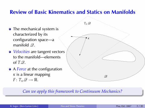
The mechanical system ischaracterized by itsconfiguration space—amanifold Q.

Velocities are tangent vectorsto the manifold—elementsof TQ.

A Force at the configurationκ is a linear mappingF : TκQ → R.

73'

&

$

%

Review of Basic Kinematics and Statics on Manifolds

• The mechanical system ischaracterized by its con-figuration space—a man-ifold Q.

• Velocities are tangent vec-tors to the manifold—elements of TQ.

• A Force at the configura-tion κ is a linear mappingF : TκQ → R.

Q

κ

TκQ

Can we apply this framework to Continuum Mechanics?

Reuven Segev: Geometric Methods, March 2001

Can we apply this framework to Continuum Mechanics?


Problems Associated with the Configuration Space

in Continuum Mechanics

What is a configuration?

Does the configuration space have a structure of a manifold?

The configuration space for continuum mechanics is infinitedimensional.


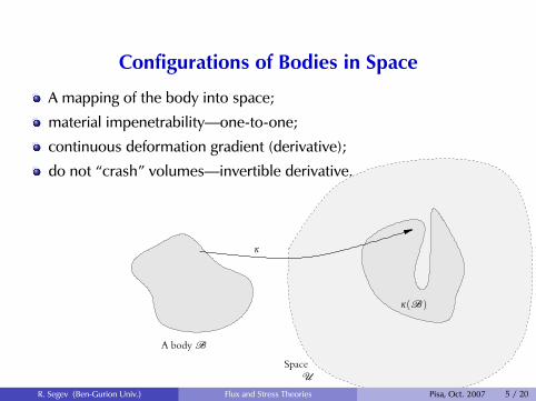
Configurations of Bodies in Space

A mapping of the body into space;

material impenetrability—one-to-one;

continuous deformation gradient (derivative);

do not “crash” volumes—invertible derivative.

75'

&

$

%

Configurations of Bodies in Space

• A mapping of the body into space;

• material impenetrability—one-to-one;

• continuous deformation gradient (derivative);

• do not “crash” volumes—invertible derivative.

U

κ

κ(B)

Space

A body B



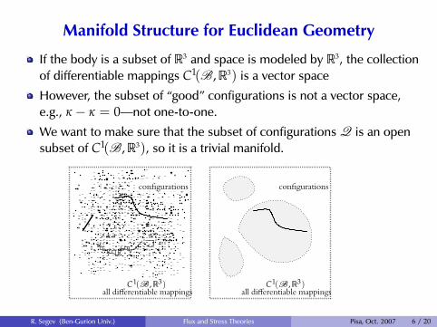
Manifold Structure for Euclidean Geometry

If the body is a subset of R3 and space is modeled by R3, the collectionof differentiable mappings C1(B,R3) is a vector space

However, the subset of “good” configurations is not a vector space,e.g., κ − κ = 0—not one-to-one.

We want to make sure that the subset of configurations Q is an opensubset of C1(B,R3), so it is a trivial manifold.

76'

&

$

%

Manifold Structure for Euclidean Geometry

• If the body is a subset of R3 and space is modeled by R3, thecollection of dicerentiable mappings C1(B,R3) is a vector space

• However, the subset of “good” configurations is not a vectorspace, e.g., κ − κ = 0—not one-to-one.

• We want to make sure that the subset of configurations Q is anopen subset of C1(B,R3), so it is a trivial manifold.

all dicerentiable mappings all dicerentiable mappingsC1(B,R3) C1(B,R3)

configurations configurations

Reuven Segev: Geometric Methods, March 2001R. Segev (Ben-Gurion Univ.) Flux and Stress Theories Pisa, Oct. 2007 6 / 20

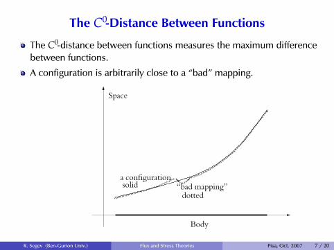
The C0-Distance Between Functions

The C0-distance between functions measures the maximum differencebetween functions.

A configuration is arbitrarily close to a “bad” mapping.

77'

&

$

%


• The C0-distance between functions measures the maximumdicerence between functions.

• A configuration is arbitrarily close to a “bad” mapping.

Space

Body

a configuration“bad mapping”

dottedsolid




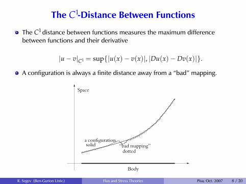
The C1 distance between functions measures the maximum differencebetween functions and their derivative

|u− v|C1 = sup{|u(x)− v(x)|, |Du(x)−Dv(x)|}.

A configuration is always a finite distance away from a “bad” mapping.

77'

&

$

%


• The C0-distance between functions measures the maximumdicerence between functions.

• A configuration is arbitrarily close to a “bad” mapping.

Space

Body

a configuration“bad mapping”

dottedsolid



Conclusions for R3

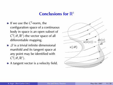
If we use the C1-norm, theconfiguration space of a continuousbody in space is an open subset ofC1(B,R3)-the vector space of alldifferentiable mapping.

Q is a trivial infinite dimensionalmanifold and its tangent space atany point may be identified withC1(B,R3).

A tangent vector is a velocity field.

79'

&

$

%

Conclusions for R3

• If we use the C1-norm, theconfiguration space of a con-tinuous body in space is anopen subset of C1(B,R3)-thevector space of all diceren-tiable mapping.

• Q is a trivial infinite dimen-sional manifold and its tan-gent space at any point may beidentified with C1(B,R3).

• A tangent vector is a velocityfield.

u(κ(x)) =dκ(x)

dtκ{B}



For Manifolds

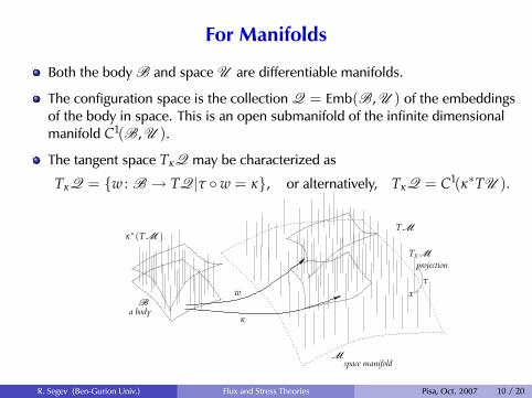
Both the body B and space U are differentiable manifolds.

The configuration space is the collection Q = Emb(B, U ) of the embeddingsof the body in space. This is an open submanifold of the infinite dimensionalmanifold C1(B, U ).

The tangent space TκQ may be characterized as

TκQ = {w : B → TQ|τ ◦w = κ}, or alternatively, TκQ = C1(κ∗TU ).

80'

&

$

%

For Manifolds• Both the body B and space U are dicerentiable manifolds.

• The configuration space is the collection Q = Emb(B, U ) of theembeddings of the body in space. This is an open submanifold of theinfinite dimensional manifold C1(B, U ).

• The tangent space TκQ may be characterized asTκQ = {w : B → TQ|τ ◦w = κ}, or alternatively, TκQ = C1(κ∗TU ).

κ

Ba body

space manifold

projection

xτ

w

M

TM

TxM

κ∗(TM)


Representation of C0-Functionals by Integrals

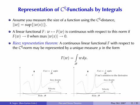
Assume you measure the size of a function using the C0-distance,‖w‖ = sup{|w(x)|}.

A linear functional F : w 7→ F(w) is continuous with respect to this norm ifF(w) → 0 when max |w(x)| → 0.

Riesz representation theorem: A continuous linear functional F with respect tothe C0-norm may be represented by a unique measure µ in the form

F(w) =∫B

w dµ.

81'

&

$

Velocity

force densityφ

w

Body B

δ

F(w) =∫

Bwφdx

force densityφ

Body B

δ

F(w) =∫

Bwφdx

Velocityw

F isn’t sensitive to the derivative


Representation of C1-Functionals by Integrals

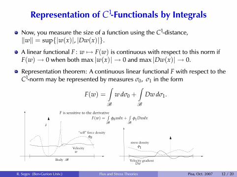
Now, you measure the size of a function using the C1-distance,‖w‖ = sup{|w(x)|, |Dw(x)|}.

A linear functional F : w 7→ F(w) is continuous with respect to this norm ifF(w) → 0 when both max |w(x)| → 0 and max |Dw(x)| → 0.

Representation theorem: A continuous linear functional F with respect to theC1-norm may be represented by measures σ0, σ1 in the form

F(w) =∫B

w dσ0 +∫B

Dw dσ1.

82'

&

$

%

Representation of C1-Functionals by Integrals• Now, you measure the size of a function using the C1-distance,‖w‖ = sup{|w(x)|, |Dw(x)|}.

• A linear functional F : w 7→ F(w) is continuous with respect to this normif F(w) → 0 when both max |w(x)| → 0 and max |Dw(x)| → 0.

• Representation theorem: A continuous linear functional F with respect tothe C1-norm may be represented by measures σ0, σ1 in the form

F(w) =∫

B

w dσ0 +∫

B

Dw dσ1.

Body B

δ

F is sensitive to the derivative

φ0

F(w) =∫B

φ0wdx +∫B

φ1 Dwdx

stress densityφ1

“self” force density

Velocity gradientDw

Velocityw


Non-Uniqueness of C1-Representation by Integrals

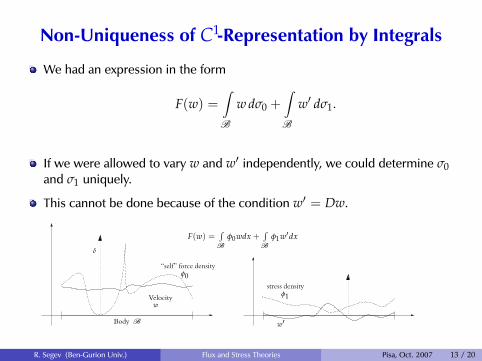
We had an expression in the form

F(w) =∫B

w dσ0 +∫B

w′ dσ1.

If we were allowed to vary w and w′ independently, we could determine σ0and σ1 uniquely.

This cannot be done because of the condition w′ = Dw.

83'

&

$

%

Non-Uniqueness of C1-Representation by Integrals

• We had an expression in the form

F(w) =∫

B

w dσ0 +∫

B

w′ dσ1.

• If we were allowed to vary w and w′ independently, we could determine

σ0 and σ1 uniquely.

• This cannot be done because of the condition w′ = Dw.

Body B

δ

φ0stress density

φ1

“self” force density

Velocityw

w′

F(w) =∫B

φ0wdx +∫B

φ1w′dx



Unique Representation of a Force System

Assume we have a force system, i.e., a force FP for every subbody P of B.

We can approximate pairs of non-compatible functions w and w′, i.e.,w′ 6= Dw, by piecewise compatible functions.

84'

&

$

%

Unique Representation of a Force System• Assume we have a force system, i.e., a force FP for every subbody P of

B.

• We can approximate pairs of non-compatible functions w and w′, i.e.,w′ 6= Dw, by piecewise compatible functions.

P1P2

P1P2

Body B

Body B

w

w′

. . . . . .

. . . . . .

∫B wdσ0

approximation of

approximation of∫B w′dσ1

∫B wdσ0

∫B w′dσ1Calculate

Calculate

• This way the two measures are determined uniquely.

• One needs consistency conditions for the force system.


This way the two measures are determined uniquely.

One needs consistency conditions for the force system.


Generalized Cauchy Consistency Conditions

85'

&

$

%


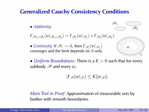
• Additivity:

FP1∪P2 (w|P1∪P2 ) = FP1 (w|P1 )+ FP2 (w|P2 ).

• Continuity: If Pi → A, then FPi (w|P1 )converges and the limit depends on A only.

P2

P1

Pi

A

• Uniform Boundedness: There is a K > 0 such that for every subbodyP and every w,

|FP (w|P ) ≤ K‖wP‖.

Main Tool in Proof: Approximation of measurable sets by bodieswith smooth boundaries.


• Additivity:

FP1∪P2(w|P1∪P2

) = FP1(w|P1

)+ FP2(w|P2

).

• Continuity: If Pi → A, then FPi(w|P1

)converges and the limit depends on A only.

85'

&

$

%


• Additivity:

FP1∪P2 (w|P1∪P2 ) = FP1 (w|P1 )+ FP2 (w|P2 ).

• Continuity: If Pi → A, then FPi (w|P1 )converges and the limit depends on A only.

P2

P1

Pi

A

• Uniform Boundedness: There is a K > 0 such that for every subbodyP and every w,

|FP (w|P ) ≤ K‖wP‖.

Main Tool in Proof: Approximation of measurable sets by bodieswith smooth boundaries.


• Uniform Boundedness: There is a K > 0 such that for everysubbody P and every w,

|FP(w|P) ≤ K‖wP‖.

Main Tool in Proof: Approximation of measurable sets bybodies with smooth boundaries.


Generalizations

All the above may be formulated and proved for differentiablemanifolds.

This formulation applies to continuum mechanics of order k > 1 (stresstensors of order k). One should simply use the Ck-norm instead of theC1-norm.

The generalized Cauchy conditions also apply to continuum mechanicsof order k > 1. This is the only formulation of Cauchy conditions forhigher order continuum mechanics.


Locality and Continuity in Constitutive Theory


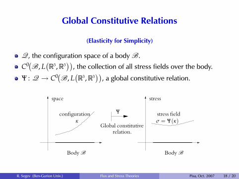
Global Constitutive Relations

(Elasticity for Simplicity)

Q, the configuration space of a body B.

C0(B, L(R3,R3

)), the collection of all stress fields over the body.

Ψ : Q → C0(B, L(R3,R3

)), a global constitutive relation.

88'

&

$

%

Global Constitutive Relations(Elasticity for Simplicity)

• Q, the configuration space of a body B.

• C0(B, L(R3,R3

)), the collection of all stress fields over the body.

• Ψ : Q → C0(B, L(R3,R3

)), a global constitutive relation.

space

Body B

configurationκ

Body B

stress

stress fieldΨ

relation.Global constitutive

σ = Ψ(κ)


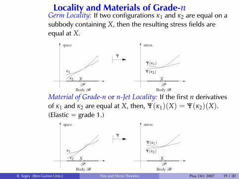
Locality and Materials of Grade-nGerm Locality: If two configurations κ1 and κ2 are equal on asubbody containing X, then the resulting stress fields areequal at X.

89'

&

$

%

Locality and Materials of Grade-nGerm Locality: If two configurations κ1 and κ2 are equal on a subbody

containing X, then the resulting stress fields are equal at X.

P

XP

X

Body B

stress

Ψ

space

Body B

κ2

κ1

Ψ(κ1)

Ψ(κ2)

Material of Grade-n or n-Jet Locality: If the first n derivatives of κ1 andκ2 are equal at X, then, Ψ(κ1)(X) = Ψ(κ2)(X). (Elastic = grade 1.)

P

XP

X

Body B

stress

Ψ

space

Body B

κ2

κ1

Ψ(κ1)

Ψ(κ2)


Material of Grade-n or n-Jet Locality: If the first n derivativesof κ1 and κ2 are equal at X, then, Ψ(κ1)(X) = Ψ(κ2)(X).(Elastic = grade 1.)

89'

&

$

%

Locality and Materials of Grade-nGerm Locality: If two configurations κ1 and κ2 are equal on a subbody

containing X, then the resulting stress fields are equal at X.

P

XP

X

Body B

stress

Ψ

space

Body B

κ2

κ1

Ψ(κ1)

Ψ(κ2)

Material of Grade-n or n-Jet Locality: If the first n derivatives of κ1 andκ2 are equal at X, then, Ψ(κ1)(X) = Ψ(κ2)(X). (Elastic = grade 1.)

P

XP

X

Body B

stress

Ψ

space

Body B

κ2

κ1

Ψ(κ1)

Ψ(κ2)



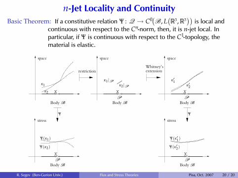
n-Jet Locality and ContinuityBasic Theorem: If a constitutive relation Ψ : Q → C0(B, L

(R3,R3

))is local and

continuous with respect to the Cn-norm, then, it is n-jet local. Inparticular, if Ψ is continuous with respect to the C1-topology, thematerial is elastic.

91'

&

$

%

κ1

κ2

P

X

space

Body B

restriction

P

X

P

X

Body B

stress

Ψ(κ′1)

Ψ(κ′2)

Ψ

P

X

space

Body B

X

space

Body B

Whitney’sextension

Ψ

Body B

stress

Ψ(κ1)

Ψ(κ2)

κ1 |Pκ2 |P

κ′1κ′2



Documents

Some Extensions and Analysis of Flux and Stress Theoryrsegev/Slides/5-GlobalApproachInVeryshort.pdf · Some Extensions and Analysis of Flux and Stress Theory Reuven Segev Department