Some Fundamentals of Observational Astronomy Kevin Krisciunas

Angular Measures Stellar Parallax Motion Across the Line of Sight

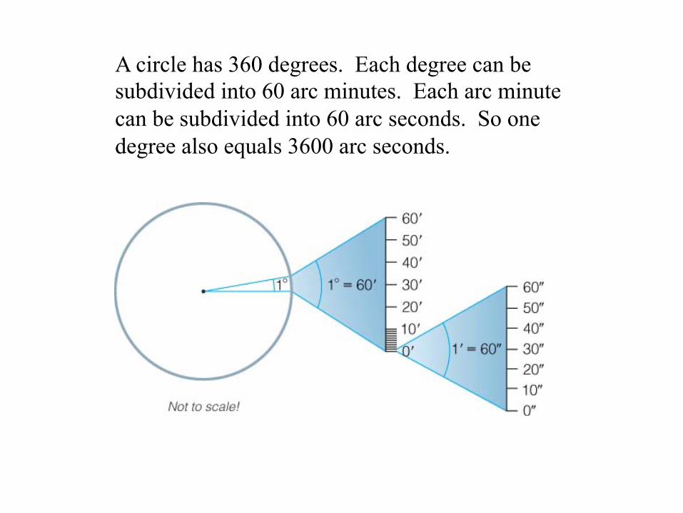
A circle has 360 degrees. Each degree can be subdivided into 60 arc minutes. Each arc minute can be subdivided into 60 arc seconds. So one degree also equals 3600 arc seconds.

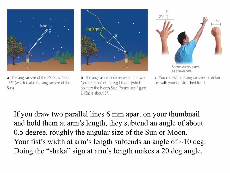
If you draw two parallel lines 6 mm apart on your thumbnail and hold them at arm’s length, they subtend an angle of about 0.5 degree, roughly the angular size of the Sun or Moon. Your fist’s width at arm’s length subtends an angle of ~10 deg. Doing the “shaka” sign at arm’s length makes a 20 deg angle.

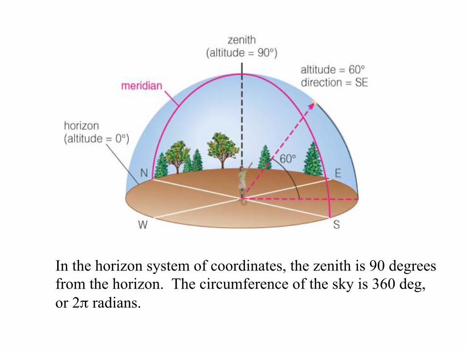
In the horizon system of coordinates, the zenith is 90 degrees from the horizon. The circumference of the sky is 360 deg, or 2π radians.

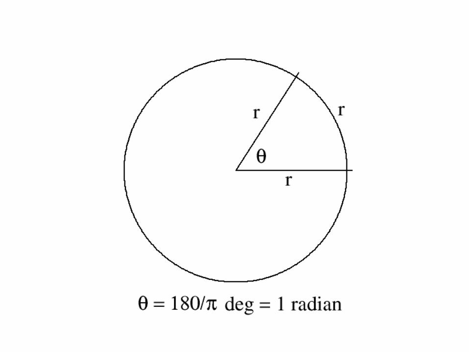
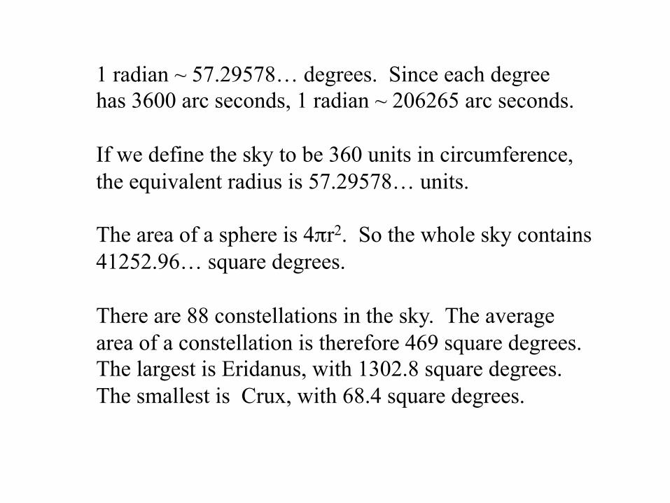
1 radian ~ 57.29578… degrees. Since each degree has 3600 arc seconds, 1 radian ~ 206265 arc seconds. If we define the sky to be 360 units in circumference, the equivalent radius is 57.29578… units. The area of a sphere is 4πr2. So the whole sky contains 41252.96… square degrees. There are 88 constellations in the sky. The average area of a constellation is therefore 469 square degrees. The largest is Eridanus, with 1302.8 square degrees. The smallest is Crux, with 68.4 square degrees.

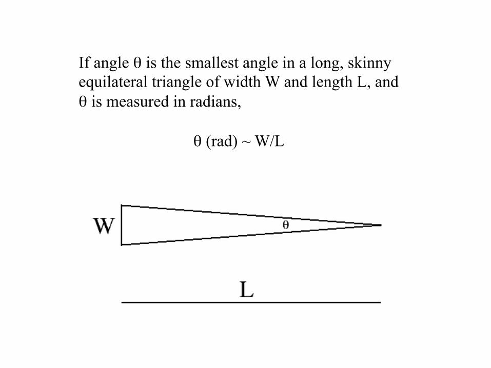
If angle θ is the smallest angle in a long, skinny equilateral triangle of width W and length L, and θ is measured in radians, θ (rad) ~ W/L

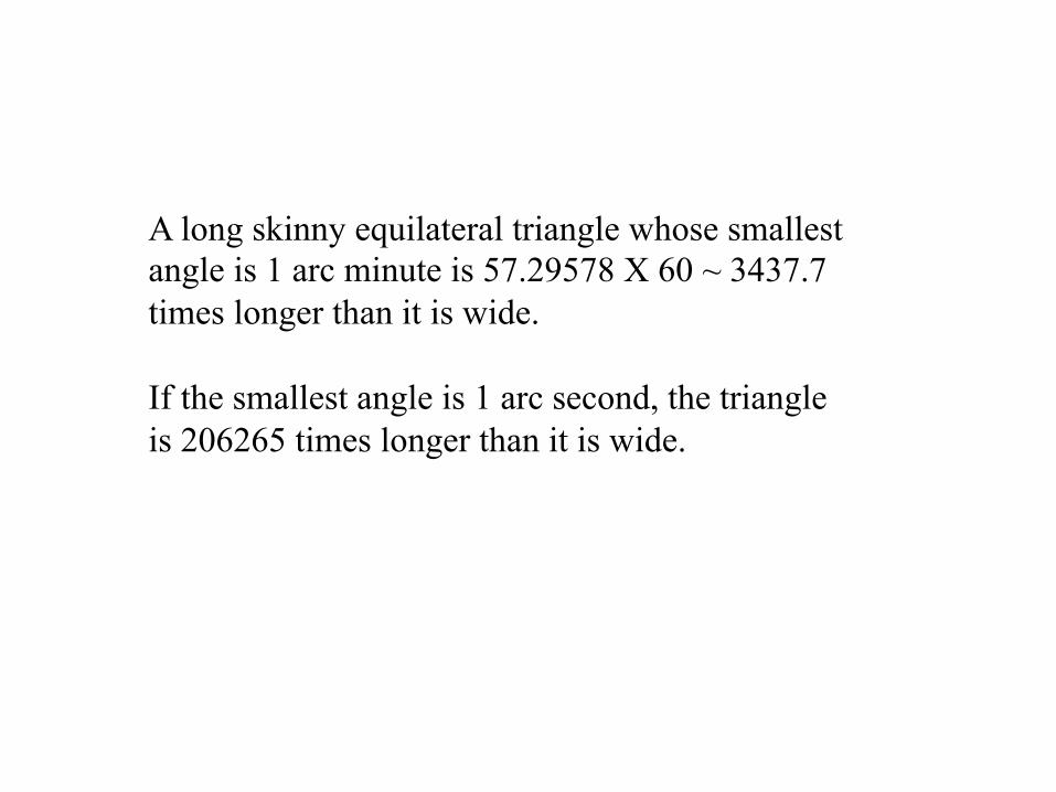
A long skinny equilateral triangle whose smallest angle is 1 arc minute is 57.29578 X 60 ~ 3437.7 times longer than it is wide. If the smallest angle is 1 arc second, the triangle is 206265 times longer than it is wide.

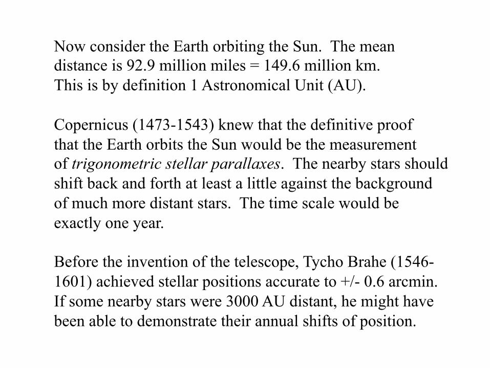
Now consider the Earth orbiting the Sun. The mean distance is 92.9 million miles = 149.6 million km. This is by definition 1 Astronomical Unit (AU). Copernicus (1473-1543) knew that the definitive proof that the Earth orbits the Sun would be the measurement of trigonometric stellar parallaxes. The nearby stars should shift back and forth at least a little against the background of much more distant stars. The time scale would be exactly one year. Before the invention of the telescope, Tycho Brahe (1546- 1601) achieved stellar positions accurate to +/- 0.6 arcmin. If some nearby stars were 3000 AU distant, he might have been able to demonstrate their annual shifts of position.

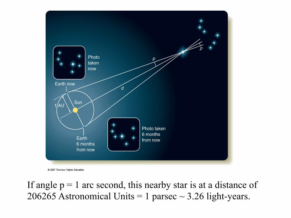
If angle p = 1 arc second, this nearby star is at a distance of 206265 Astronomical Units = 1 parsec ~ 3.26 light-years.

The measurement of stellar parallax was not achieved until the 1830’s because the nearest stars other than the Sun are hundreds of thousands of AU distant. The required positional accuracy had to be ~0.1 arcsec or better. The closest known star other than the Sun is Proxima Centauri, which is 4.3 light-years away. It only shifts back and forth +/- ¾ of an arc second over the course of the year. Incidentally, the word “parsec” is a contraction of “parallax of 1 second of arc”.

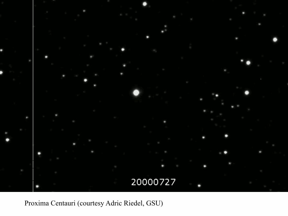
Proxima Centauri (courtesy Adric Riedel, GSU)

There is a simple relationship between the distance to a star in parsecs and its trigonometric stellar parallax: d (pc) = 1/p (arcsec) With a satellite operating outside the Earth’s atmosphere we can measure parallaxes to about +/- 0.001 arcsec. The limiting distance is about 300 pc.

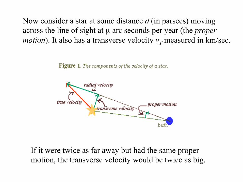
Now consider a star at some distance d (in parsecs) moving across the line of sight at µ arc seconds per year (the proper motion). It also has a transverse velocity vT measured in km/sec.

If it were twice as far away but had the same proper motion, the transverse velocity would be twice as big.

The relationship between transverse velocity and proper motion is as follows: vT = 4.74 d µ The scale factor comes from: (km/sec) / [parsecs x arcsec/yr] = (km/pc) / [(sec/yr) x (arcsec/radian)] = (206265 x 149.6 X 106) / [3.156 X 107 x 206265]~ 4.74. A star at a distance of 10 pc that has a proper motion of 1 arcsec/yr has a transverse velocity of 47.4 km/sec.

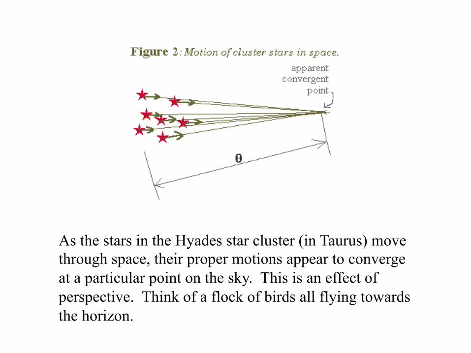
As the stars in the Hyades star cluster (in Taurus) move through space, their proper motions appear to converge at a particular point on the sky. This is an effect of perspective. Think of a flock of birds all flying towards the horizon.

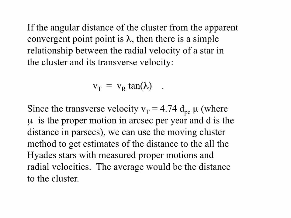
If the angular distance of the cluster from the apparent convergent point point is λ, then there is a simple relationship between the radial velocity of a star in the cluster and its transverse velocity: vT = vR tan(λ) . Since the transverse velocity vT = 4.74 dpc µ (where µ  is the proper motion in arcsec per year and d is the distance in parsecs), we can use the moving cluster method to get estimates of the distance to the all the Hyades stars with measured proper motions and radial velocities. The average would be the distance to the cluster.

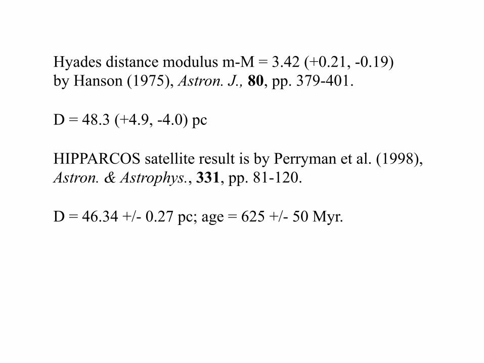
Hyades distance modulus m-M = 3.42 (+0.21, -0.19) by Hanson (1975), Astron. J., 80, pp. 379-401. D = 48.3 (+4.9, -4.0) pc HIPPARCOS satellite result is by Perryman et al. (1998), Astron. & Astrophys., 331, pp. 81-120. D = 46.34 +/- 0.27 pc; age = 625 +/- 50 Myr.

Stellar Magnitudes The relationship between absolute magnitude, apparent magnitude and distance

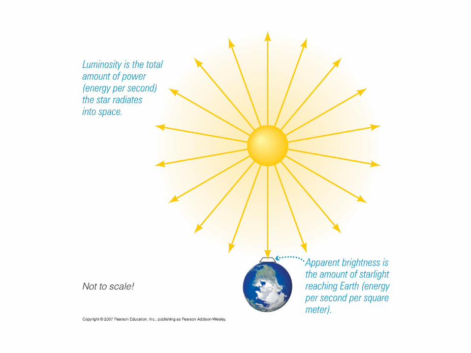
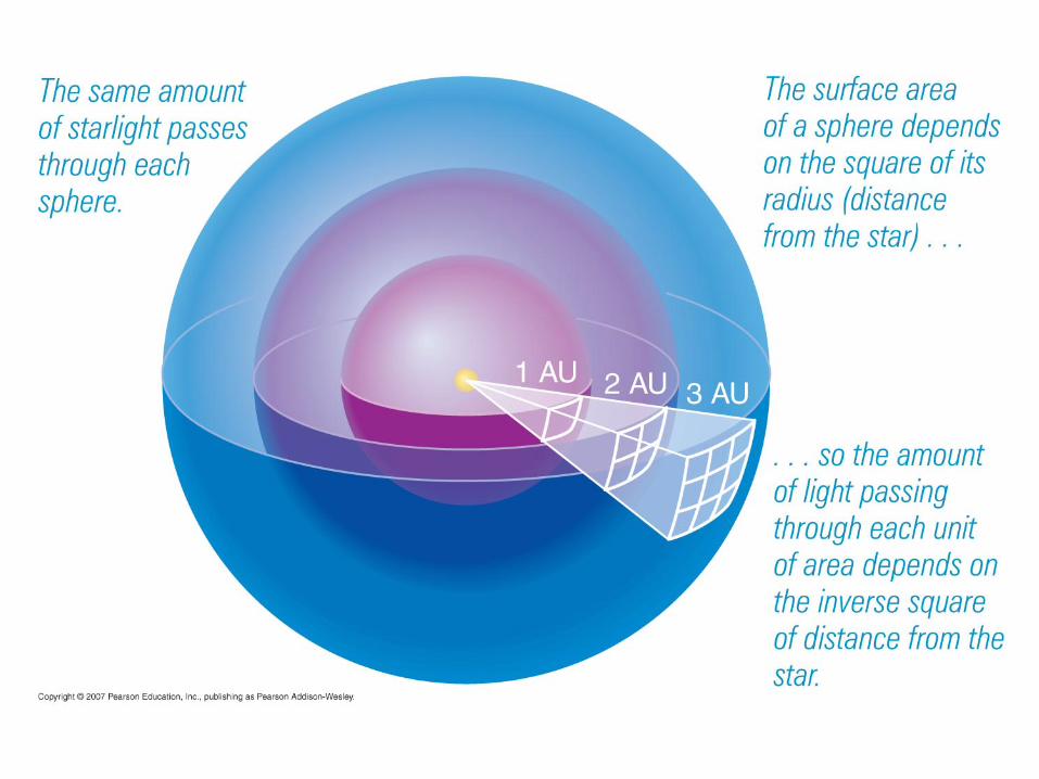
It is important to remember what we actually measure when we measure the brightness of a star. We do not measure the luminosity. We measure the apparent brightness. The apparent brightness of a star decreases with the square of the distance because the area of a sphere increases with the square of the distance. We wish to obtain an expression that relates some measure of the intrinsic brightness (i.e. luminosity) with the apparent brightness and the distance.

Hipparchus lived on the Island of Rhodes in the eastern Mediterranean during the 2nd century BC. He put together a catalog of the positions and brightnesses of about 1000 stars visible at that latitude. This catalog was reproduced in Ptolemy’s Almagest in the 2nd century AD, with the ecliptic longitudes corrected for something called the precession of the equinoxes. Hipparchus divided the stars into logarithmic categories of brightness – stellar magnitudes. The brightest stars are stars of the first class, or 1st magnitude stars. The 2nd magnitude stars are about 2.5 times fainter. The 3rd magnitude stars are ~2.5 times fainter still.

In the 19th and 20th centuries the magnitude scale was more exactly defined. Consider two stars. Say one gives us a certain number of photons/sec in some photometric band (L1) while the other star gives us L2 (100 times smaller than L1). The fainter star is exactly 5 magnitudes fainter. (m2 is further to the right on the number line compared to m1). If the apparent magnitudes of these stars are m1 and m2 , we have, in general: m2 – m1 = 2.5 log (L1 / L2 ) and L1 / L2 = 2.511886 (m2 - m1)

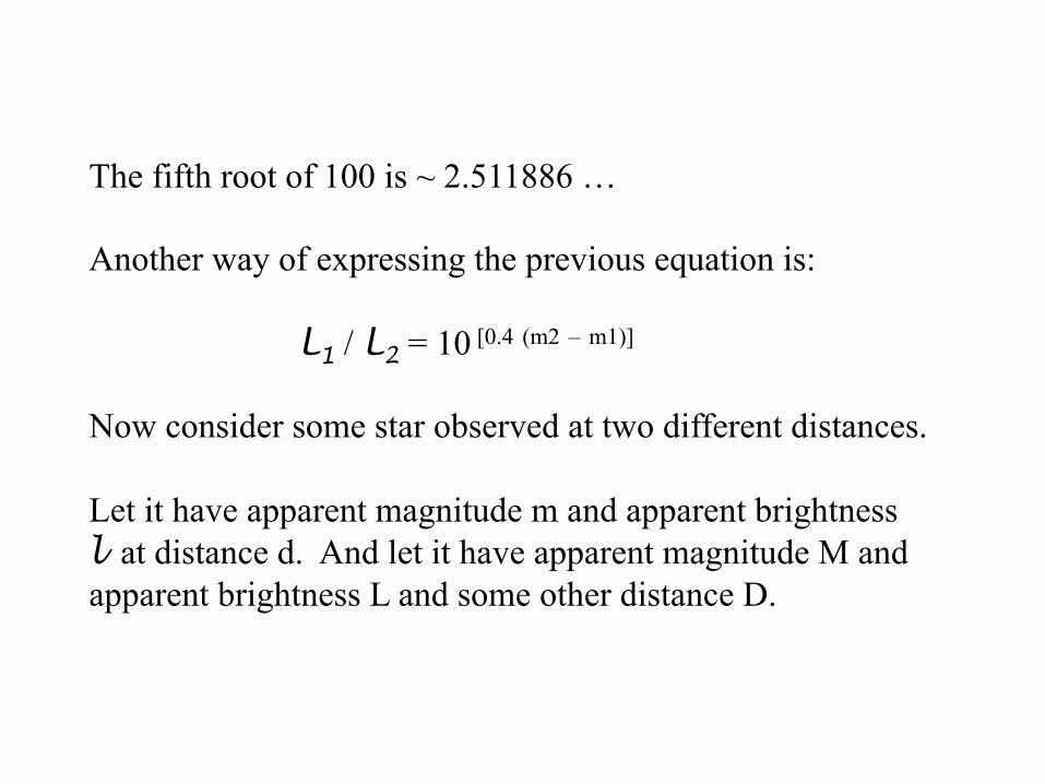
The fifth root of 100 is ~ 2.511886 … Another way of expressing the previous equation is: L1 / L2 = 10 [0.4 (m2 – m1)] Now consider some star observed at two different distances. Let it have apparent magnitude m and apparent brightness l at distance d. And let it have apparent magnitude M and apparent brightness L and some other distance D.

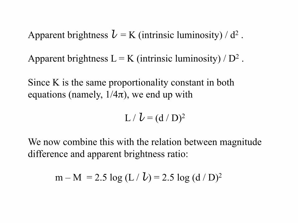
Apparent brightness l = K (intrinsic luminosity) / d2 . Apparent brightness L = K (intrinsic luminosity) / D2 . Since K is the same proportionality constant in both equations (namely, 1/4π), we end up with L / l = (d / D)2

We now combine this with the relation between magnitude difference and apparent brightness ratio: m – M = 2.5 log (L / l ) = 2.5 log (d / D)2

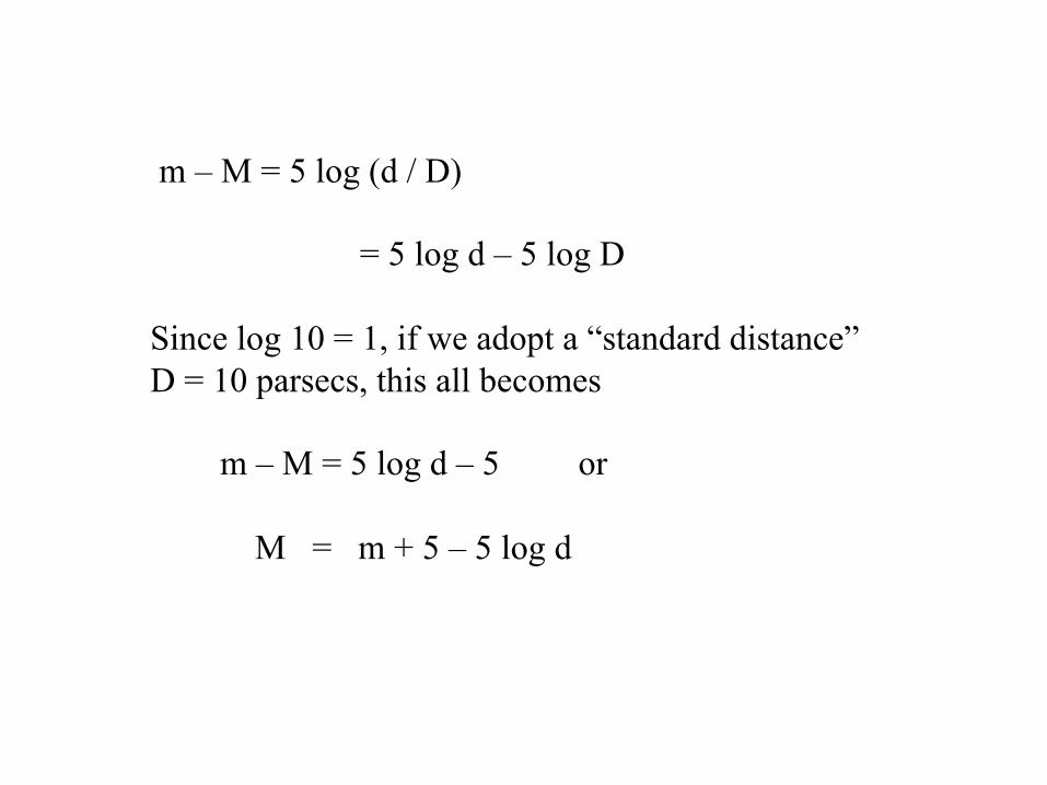
m – M = 5 log (d / D) = 5 log d – 5 log D Since log 10 = 1, if we adopt a “standard distance” D = 10 parsecs, this all becomes m – M = 5 log d – 5 or M = m + 5 – 5 log d

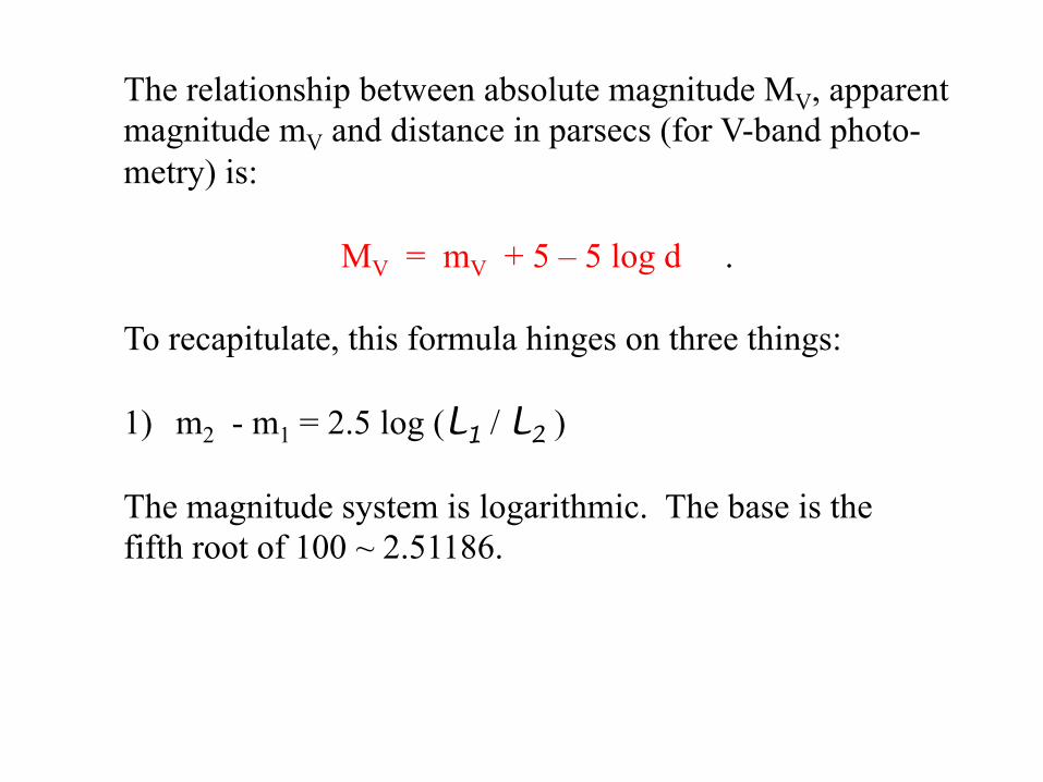
The relationship between absolute magnitude MV, apparent magnitude mV and distance in parsecs (for V-band photo- metry) is: MV = mV + 5 – 5 log d . To recapitulate, this formula hinges on three things: 1)  m2 - m1 = 2.5 log (L1 / L2 )

The magnitude system is logarithmic. The base is the fifth root of 100 ~ 2.51186.

2) apparent brightness decreases with the square of the distance 3)  the “standard distance” for absolute mags is 10 pc

Absolute magnitude is the apparent magnitude an object would have if it were at 10 parsecs. The “distance modulus” is m – M = 5 log d – 5 . In these last two formulae the apparent magnitude has been corrected for any dimming effects of interstellar dust.

The Sun’s absolute visual magnitude is +4.8. How faint would a star like the Sun be at d = 100 pc? You can actually do this in your head. 100 pc is 10 times the standard distance of 10 pc related to the definition of absolute magnitudes. Light decreases with the square of the distance. From 10 times further away you get 1/100 of the light, which corresponds to a difference of 5 magnitudes. So the Sun would be mV = +9.8 at 100 pc, and +14.8 at 1000 pc. (Any effect of dust extinction would make these apparent magnitudes fainter.)

Now imagine you were observing a star cluster whose distance was 1000 pc. An A0 main sequence star has an intrinsic color of B-V = 0.0, and because its absolute magnitude is ~0.0, it should have V ~ 10.0. But what if this cluster was in the Galactic plane and the stars’ light was affected by interstellar dust along the line of sight? Our A0 main sequence star might have V = 13.0 and B = 14.0. Its observed B-V color would be 1.0, not 0.0. It has a color excess of E(B-V) = 1.0 mag, AV = 3.0 mag and AB = 4.0 mag. AV / E(B-V) ~ 3.

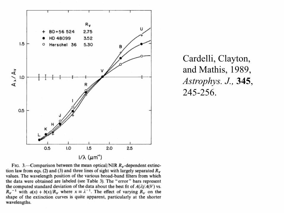
Cardelli, Clayton, and Mathis, 1989, Astrophys. J., 345, 245-256.

The B-band extinction is greater than the V-band extinction. If the color excess is E(B-V), we define AV = RV E(B-V) . A typical value of RV is 3.1 for Milky Way dust. BUT values in our Galaxy can range from 2.3 to 5.5 along various lines of sight. Evidence from supernovae can reveal values smaller than 2.0, owing to dust in their host galaxies and circumstellar scattering.

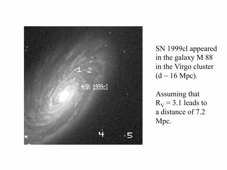
SN 1999cl appeared in the galaxy M 88 in the Virgo cluster (d ~ 16 Mpc). Assuming that RV = 3.1 leads to a distance of 7.2 Mpc.

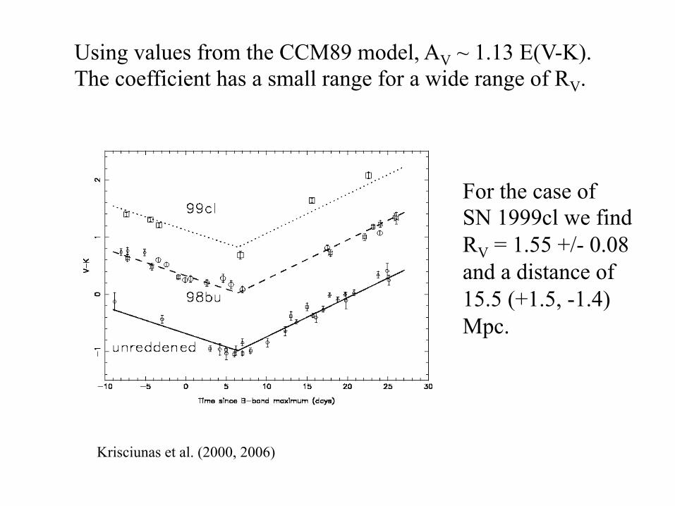
For the case of SN 1999cl we find RV = 1.55 +/- 0.08 and a distance of 15.5 (+1.5, -1.4) Mpc.

Using values from the CCM89 model, AV ~ 1.13 E(V-K). The coefficient has a small range for a wide range of RV.

Krisciunas et al. (2000, 2006)

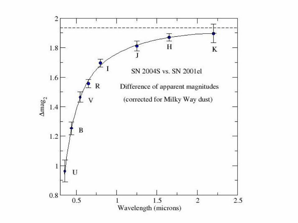
Now imagine two identical Type Ia supernovae in different galaxies at different distances. If there is no dust along either line of sight, a difference of the brightness in any photometric band (at the same Number of days after T(Bmax)) will give the difference of the distance moduli (m-M). In the case of SNe 2001el and 2004S we seem to have two “clones”. But the photometry shows that SN 2001el is fainter and fainter compared to SN 2004S as we proceed from the near-IR to the near-UV.

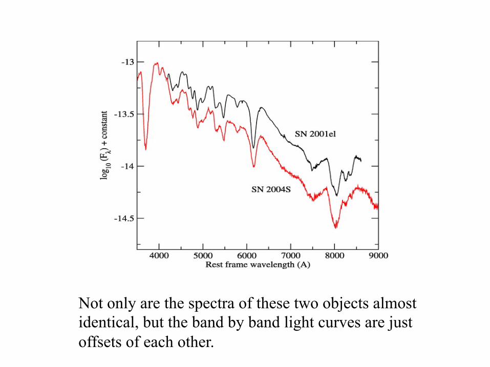
Not only are the spectra of these two objects almost identical, but the band by band light curves are just offsets of each other.

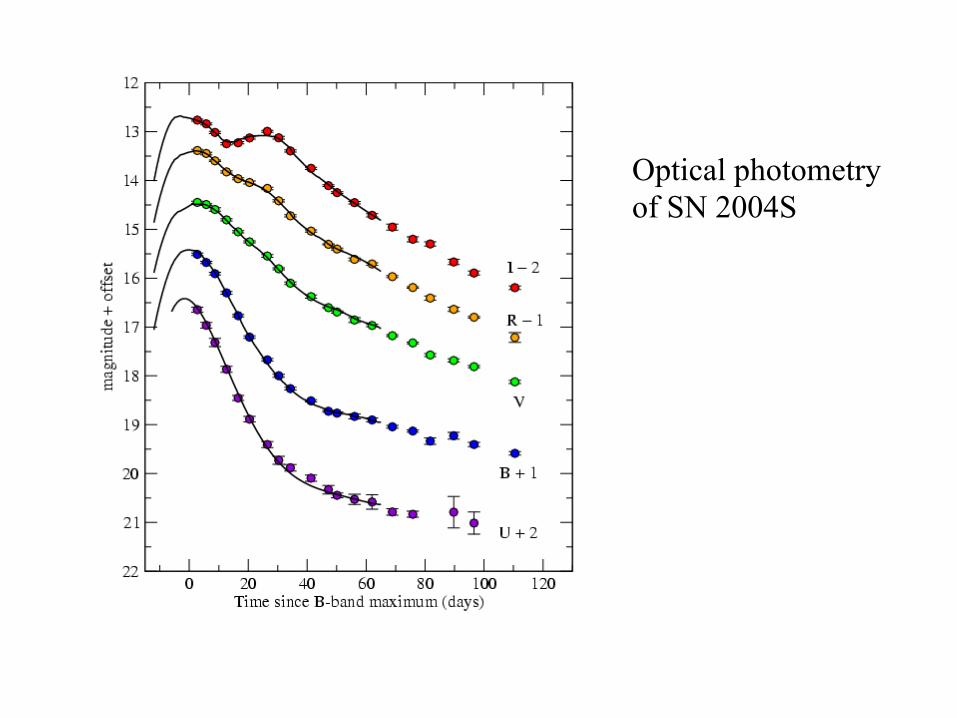
Optical photometry of SN 2004S

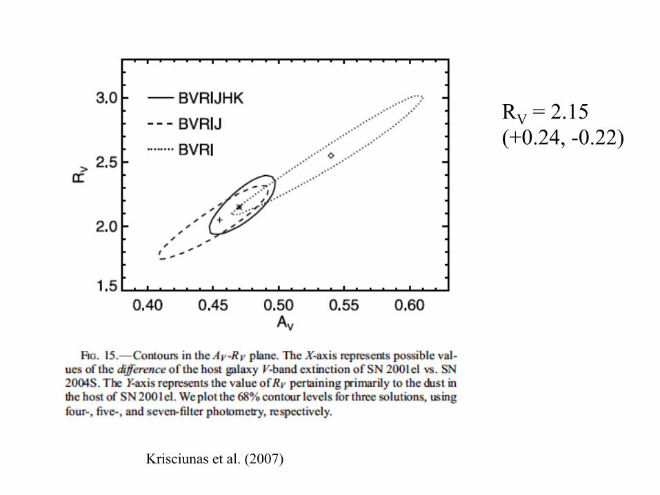
RV = 2.15 (+0.24, -0.22)

Krisciunas et al. (2007)

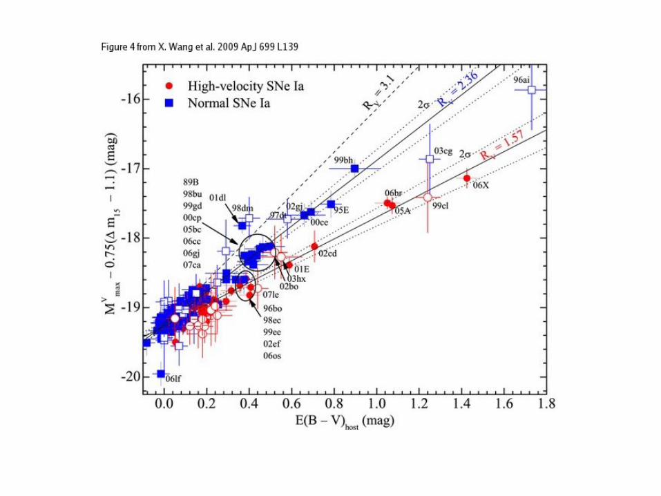
We use observations of Type Ia SNe to derive details of the kind of universe we live in (total matter density, Dark Energy density). It is found that the residuals in a Hubble diagram are minimized by using a value of RV ~ 1.7, not the value 3.1 we think applies for much of Milky Way dust. The bottom line is that corrections for dust extinction are problematic, but uncertainties are minimized by having observations in the optical and the near-IR.

The bright star Vega (in Lyra) has a V magnitude very close to 0.00, as well as the star Rigel in Orion. Sirius, the brightest star other than the Sun, has V = -1.42. By far the easiest way to get a handle on the apparent magnitude scale of the naked eye stars is to take a star chart outside and see how bright stars of different magnitudes are up in the sky. At the Texas A&M observatory, near the south end of Easterwood Airport, it’s possible to see stars of apparent magnitude 5.0 with the naked eye. In west Texas under clear, moonless skies, one can detect mag 6.0 to 6.3.

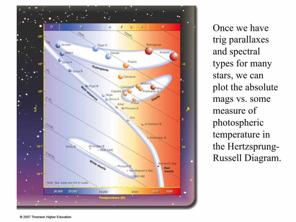
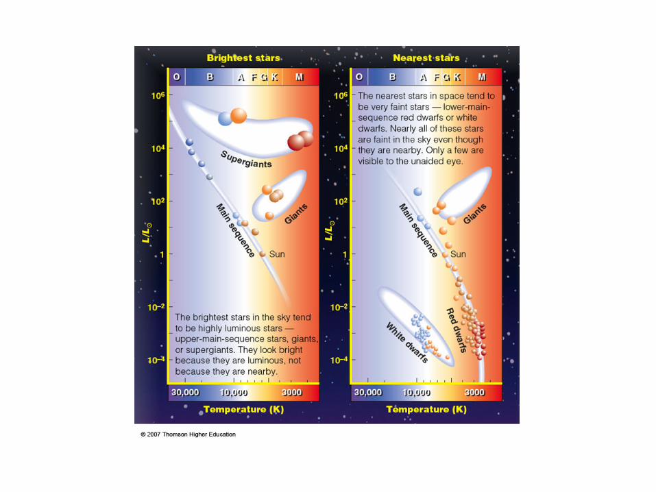
Once we have trig parallaxes and spectral types for many stars, we can plot the absolute mags vs. some measure of photospheric temperature in the Hertzsprung- Russell Diagram.

Stars on the main sequence convert protons into helium nuclei. Roughly 0.7 percent of the mass of the protons is converted to energy via Einstein’s formula E = mc2. Nuclear fusion in stars is such that the rate of energy production is a strong function of the temperature. More massive main sequence stars have hotter cores and use up their core hydrogen at a much faster rate than less massive main sequence stars. If stars in a star cluster are all formed about the same time, the hottest, brightest MS stars evolve first to become supergiants or giants. Then the slightly less massive ones, and so on.

Photometric Systems

In order to standardize measurements of brightness of stars and supernovae, we need agreed-upon standard photometric bandpasses.

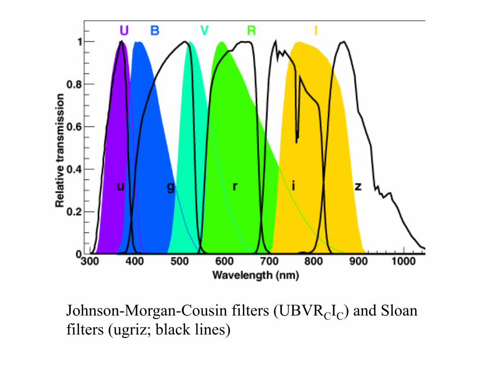
Johnson-Morgan-Cousin filters (UBVRCIC) and Sloan filters (ugriz; black lines)

Two widely used photometric systems for optical photometry: UBVRI: Landolt (1992, Astron. J., 104, pp. 340-376) Landolt (2007, Astron. J., 133, pp. 2502-2523) Sloan photometry: J. Allyn Smith et al. (2002, Astron. J., 123, pp. 2121-2144) For information on reducing aperture photometry see: people.physics.tamu.edu/krisciunas/aperture.ppt

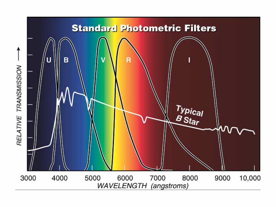
If you consider a hot star, like one of B spectral type, It gives off more energy in the B-band than in the V-band. Its B-band magnitude is brighter than its V-band magnitude, so its B-V color index is a negative number. The Sun has B-V = 0.650.* The B-V color index is a measure of photospheric temperature.

*Allen’s Astrophysical Quantities, 4th ed. ,2000, p. 341.

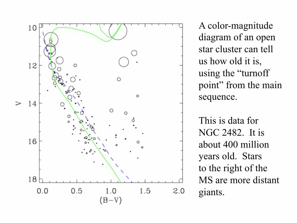
A color-magnitude diagram of an open star cluster can tell us how old it is, using the “turnoff point” from the main sequence. This is data for NGC 2482. It is about 400 million years old. Stars to the right of the MS are more distant giants.

Why is the Night Sky Dark?

Heinrich Wilhelm Olbers (1758-1840) formulated an idea known as Olbers’ Paradox. If the universe were infinite in extent, then along any line of sight we should eventually run into a star or galaxy. The night sky “should” be blindingly bright, but instead is dark. The resolution of this paradox hinges on these facts – the universe is not infinitely old, and stars do not live forever.

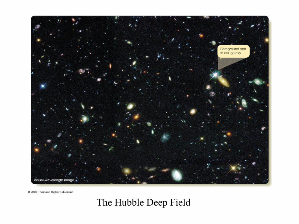
The Hubble Deep Field

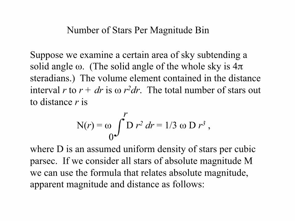
Number of Stars Per Magnitude Bin

Suppose we examine a certain area of sky subtending a solid angle ω. (The solid angle of the whole sky is 4π steradians.) The volume element contained in the distance interval r to r + dr is ω r2dr. The total number of stars out to distance r is r N(r) = ω D r2 dr = 1/3 ω D r3 , 0 where D is an assumed uniform density of stars per cubic parsec. If we consider all stars of absolute magnitude M we can use the formula that relates absolute magnitude, apparent magnitude and distance as follows:

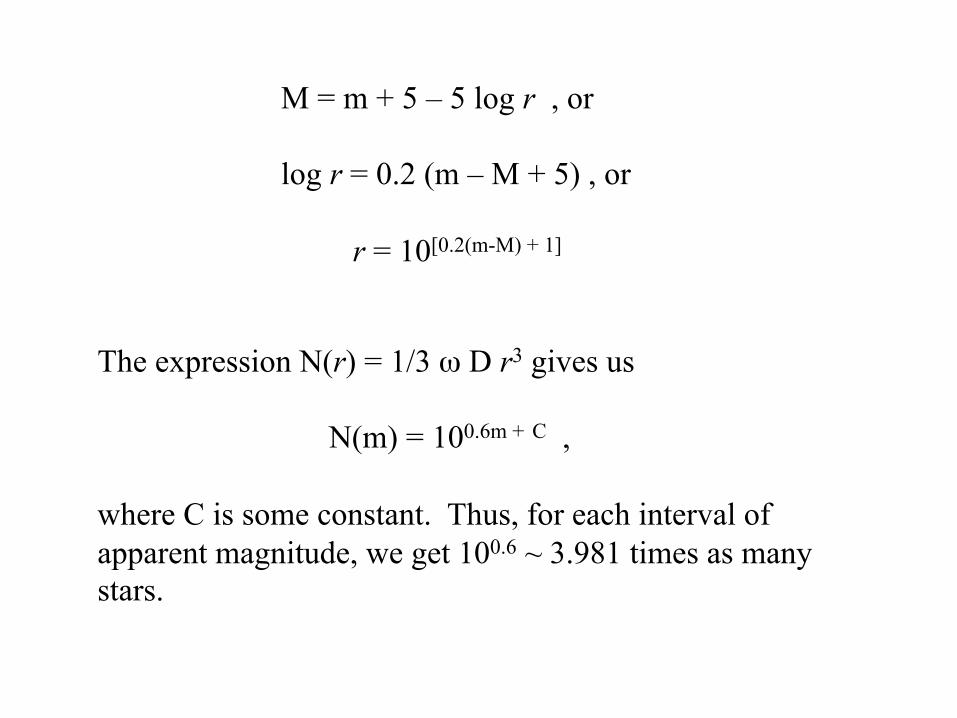
M = m + 5 – 5 log r , or log r = 0.2 (m – M + 5) , or r = 10[0.2(m-M) + 1]

The expression N(r) = 1/3 ω D r3 gives us N(m) = 100.6m + C , where C is some constant. Thus, for each interval of apparent magnitude, we get 100.6 ~ 3.981 times as many stars.

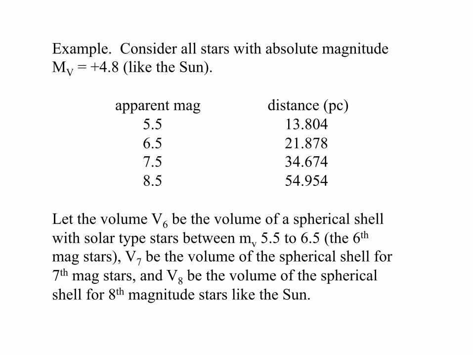
Example. Consider all stars with absolute magnitude MV = +4.8 (like the Sun). apparent mag distance (pc) 5.5 13.804 6.5 21.878 7.5 34.674 8.5 54.954 Let the volume V6 be the volume of a spherical shell with solar type stars between mv 5.5 to 6.5 (the 6th mag stars), V7 be the volume of the spherical shell for 7th mag stars, and V8 be the volume of the spherical shell for 8th magnitude stars like the Sun.

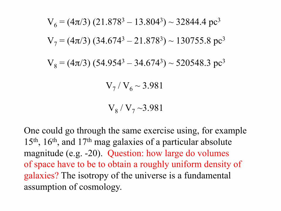
V6 = (4π/3) (21.8783 – 13.8043) ~ 32844.4 pc3

V7 = (4π/3) (34.6743 – 21.8783) ~ 130755.8 pc3 V8 = (4π/3) (54.9543 – 34.6743) ~ 520548.3 pc3 V7 / V6 ~ 3.981 V8 / V7 ~3.981 One could go through the same exercise using, for example 15th, 16th, and 17th mag galaxies of a particular absolute magnitude (e.g. -20). Question: how large do volumes of space have to be to obtain a roughly uniform density of galaxies? The isotropy of the universe is a fundamental assumption of cosmology.

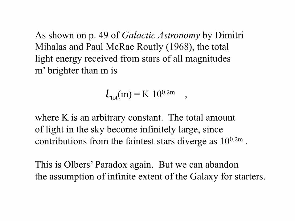
As shown on p. 49 of Galactic Astronomy by Dimitri Mihalas and Paul McRae Routly (1968), the total light energy received from stars of all magnitudes m’ brighter than m is Ltot(m) = K 100.2m , where K is an arbitrary constant. The total amount of light in the sky become infinitely large, since contributions from the faintest stars diverge as 100.2m . This is Olbers’ Paradox again. But we can abandon the assumption of infinite extent of the Galaxy for starters.

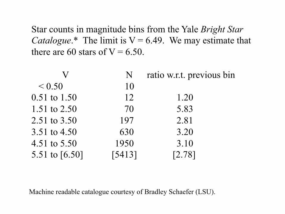
Star counts in magnitude bins from the Yale Bright Star Catalogue.* The limit is V = 6.49. We may estimate that there are 60 stars of V = 6.50. V N ratio w.r.t. previous bin < 0.50 10 0.51 to 1.50 12 1.20 1.51 to 2.50 70 5.83 2.51 to 3.50 197 2.81 3.51 to 4.50 630 3.20 4.51 to 5.50 1950 3.10 5.51 to [6.50] [5413] [2.78]

Machine readable catalogue courtesy of Bradley Schaefer (LSU).

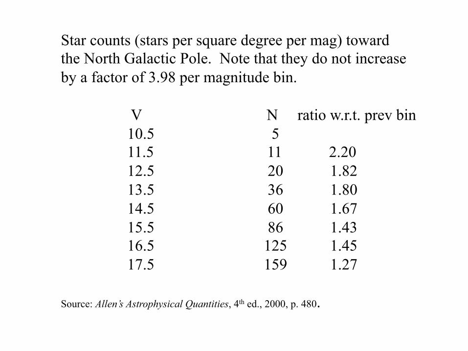
Star counts (stars per square degree per mag) toward the North Galactic Pole. Note that they do not increase by a factor of 3.98 per magnitude bin. V N ratio w.r.t. prev bin 10.5 5 11.5 11 2.20 12.5 20 1.82 13.5 36 1.80 14.5 60 1.67 15.5 86 1.43 16.5 125 1.45 17.5 159 1.27 Source: Allen’s Astrophysical Quantities, 4th ed., 2000, p. 480.

Detecting a faint astronomical object is always a contrast effect between the sky+object compared to the otherwise blank sky.

Analogy. Carrying on a conversation with someone is much easier in a library compared to in a crowded restaurant where everyone is talking.

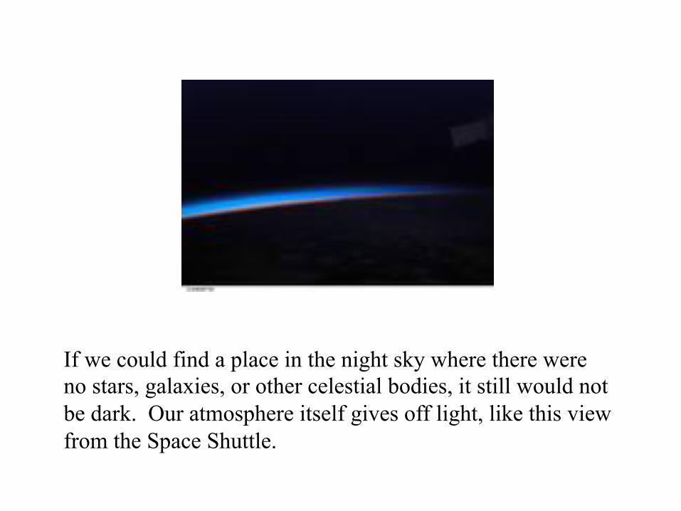
If we could find a place in the night sky where there were no stars, galaxies, or other celestial bodies, it still would not be dark. Our atmosphere itself gives off light, like this view from the Space Shuttle.

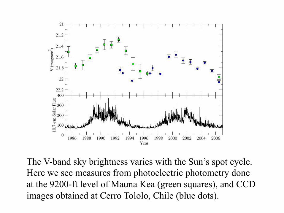
The V-band sky brightness varies with the Sun’s spot cycle. Here we see measures from photoelectric photometry done at the 9200-ft level of Mauna Kea (green squares), and CCD images obtained at Cerro Tololo, Chile (blue dots).

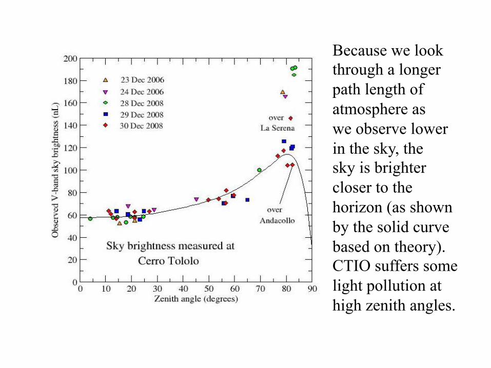
Because we look through a longer path length of atmosphere as we observe lower in the sky, the sky is brighter closer to the horizon (as shown by the solid curve based on theory). CTIO suffers some light pollution at high zenith angles.

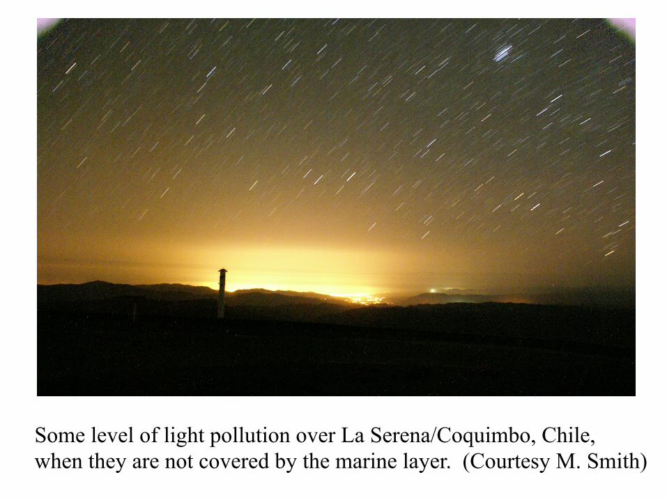
Some level of light pollution over La Serena/Coquimbo, Chile, when they are not covered by the marine layer. (Courtesy M. Smith)

Numerical example. Say we observe with the Las Campanas 1-m in Chile using its CCD camera. The “plate scale” is 0.435 arcsec per pixel. It is found that an r = 8 px aperture is adequate for data reduction of stars on nights of average seeing. The V-band sky brightness ranges from 21.2 to 21.8 mag per square arc second over the course of the solar cycle. An aperture of r = 8 px = 3.48 arcsec has an area of 38.05 square arc seconds. If we are trying to measure the brightness of a faint star using aperture photometry, the sky itself (on a moonless night) will be as bright as a star of magnitude V ~ -2.5 log (38.05) + 21.5 ~ 17.55 Using exposures of 300 to 600 seconds, we can measure supernovae fainter than magnitude 19 (to +/- 0.06 mag) in most bands using a 1-m telescope at a good site.

Accurate photometry hinges on obtaining a high value of the signal to noise ratio (S/N). If there is moonlight, artificial light pollution, or the Sun is at solar maximum, it becomes difficult (or impossible) to obtain accurate measurements. At IR wavelengths the sky actually emits light itself. This is why IR astronomy is best done: 1) on a tall mountain, with as much of the atmosphere below; or 2) using a satellite completely outside the atmosphere.

Doppler Shifts / Radial Velocities Cosmology

Let λ0 be the wavelength of a particular spectra line measured in the laboratory, and let λobs be the wavelength of the same line observed in some celestial body. The Doppler shift is Δλ / λ0 = (λobs – λ0) / λ0 and the radial velocity is vR = [Δλ / λ] c , where c is the velocity of light, ~300,000 km/sec.

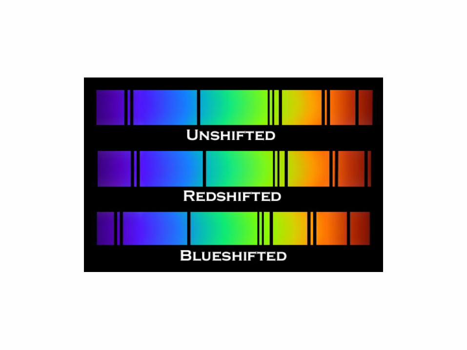
Consider the hydrogen α line (whose lab wavelength is 6563 Angstroms). If it is observed at 6564 A in a star, then that star is receding from us at 46 km/sec. If the spectral shift Δλ / λ > 0, the spectrum is redshifted and vR is positive. If the spectral shift Δλ / λ < 0, the spectrum is blueshifted and vR is negative. Except for a few very nearby galaxies, all other galaxies have redshifted spectra. Astronomers use the parameter z = Δλ / λ for the redshifts of the galaxies.

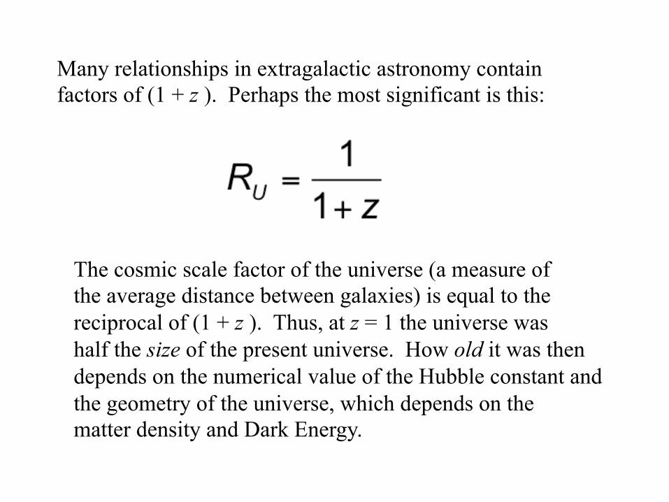
Many relationships in extragalactic astronomy contain factors of (1 + z ). Perhaps the most significant is this:

The cosmic scale factor of the universe (a measure of the average distance between galaxies) is equal to the reciprocal of (1 + z ). Thus, at z = 1 the universe was half the size of the present universe. How old it was then depends on the numerical value of the Hubble constant and the geometry of the universe, which depends on the matter density and Dark Energy.

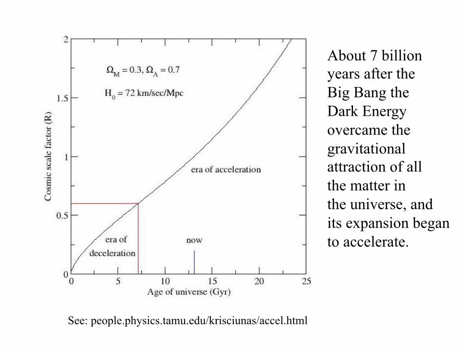
About 7 billion years after the Big Bang the Dark Energy overcame the gravitational attraction of all the matter in the universe, and its expansion began to accelerate.

See: people.physics.tamu.edu/krisciunas/accel.html

Another simple relation gives us the temperature of the cosmic microwave background (CMB) radiation as a function of redshift: T(z) = 2.73 (1 + z ) [deg K] Observations by A. Songaila (Univ. of Hawaii) of absorption lines towards a few distant quasars show that this prediction of the Big Bang theory is confirmed.

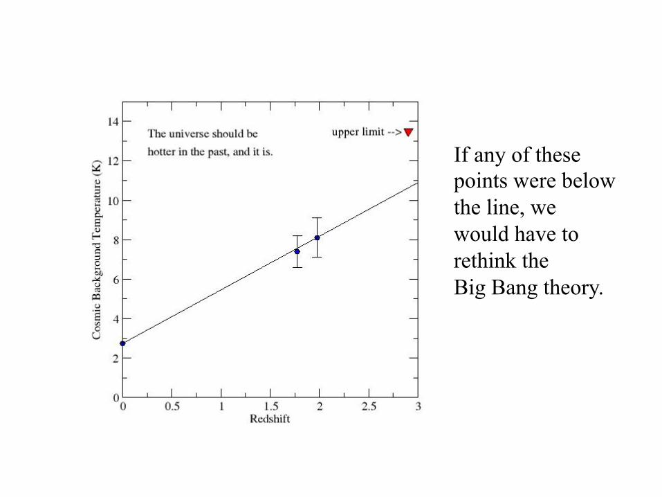
If any of these points were below the line, we would have to rethink the Big Bang theory.

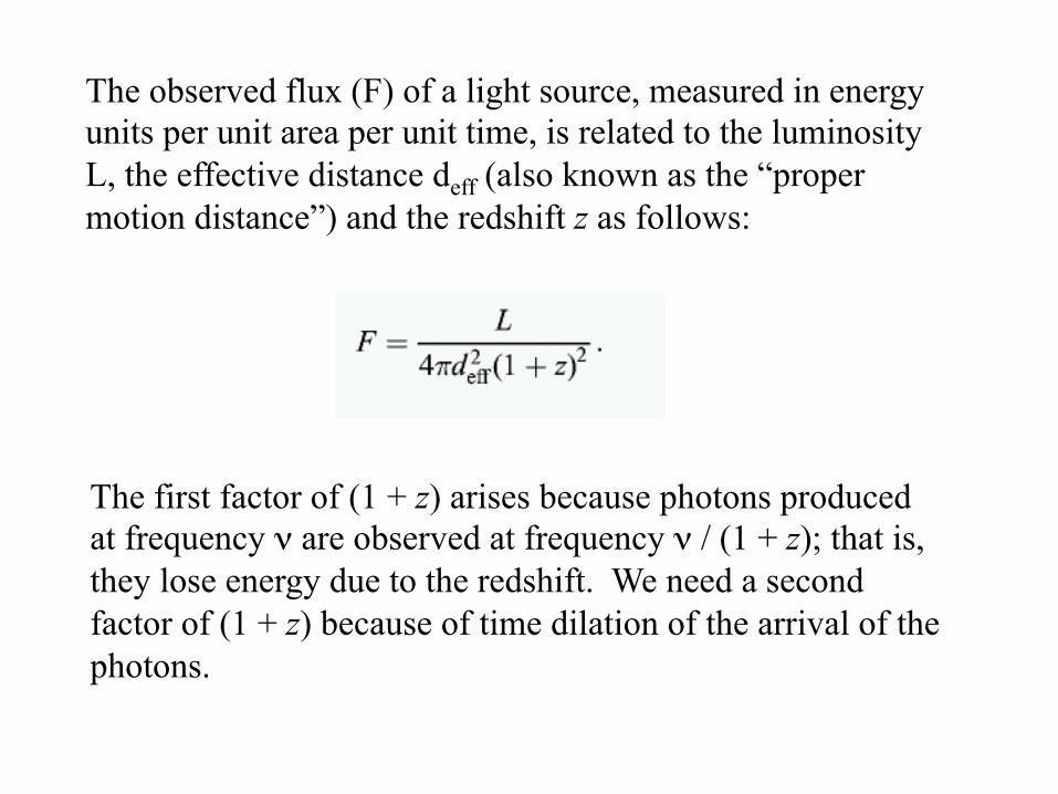
The observed flux (F) of a light source, measured in energy units per unit area per unit time, is related to the luminosity L, the effective distance deff (also known as the “proper motion distance”) and the redshift z as follows:

The first factor of (1 + z) arises because photons produced at frequency ν are observed at frequency ν / (1 + z); that is, they lose energy due to the redshift. We need a second factor of (1 + z) because of time dilation of the arrival of the photons.

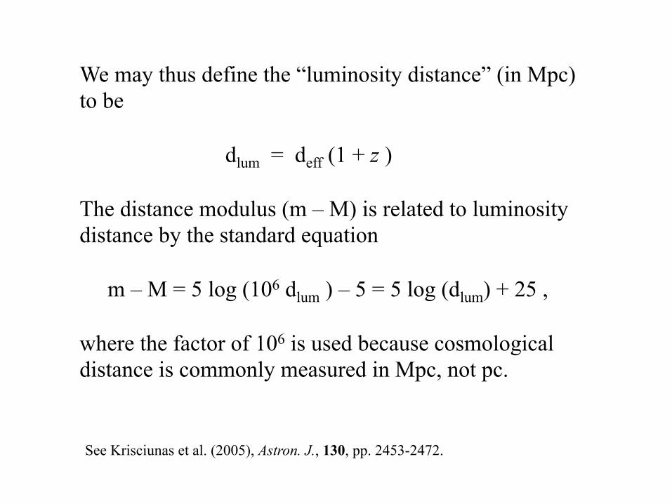
We may thus define the “luminosity distance” (in Mpc) to be dlum = deff (1 + z ) The distance modulus (m – M) is related to luminosity distance by the standard equation m – M = 5 log (106 dlum ) – 5 = 5 log (dlum) + 25 , where the factor of 106 is used because cosmological distance is commonly measured in Mpc, not pc.

See Krisciunas et al. (2005), Astron. J., 130, pp. 2453-2472.

The Tolman surface brightness test relates to the amount of light given off per unit area by galaxies. The surface brightness decreases by (1 + z )4.

Hubble’s Law Beyond a distance of roughly d ~ 20 million parsecs (Mpc) the universe is quite uniformly expanding. The velocity of recession is proportional to the distance: v (km/sec) = H0 dMpc H0 is the Hubble constant, roughly equal to 72 km/sec/Mpc (Freedman et al. 2001). Other, more recent, estimates are in the range 67 to 74. We most easily obtain the distances to faraway galaxies either using photometric measurements of Type Ia supernovae, or by means of Hubble’s Law.

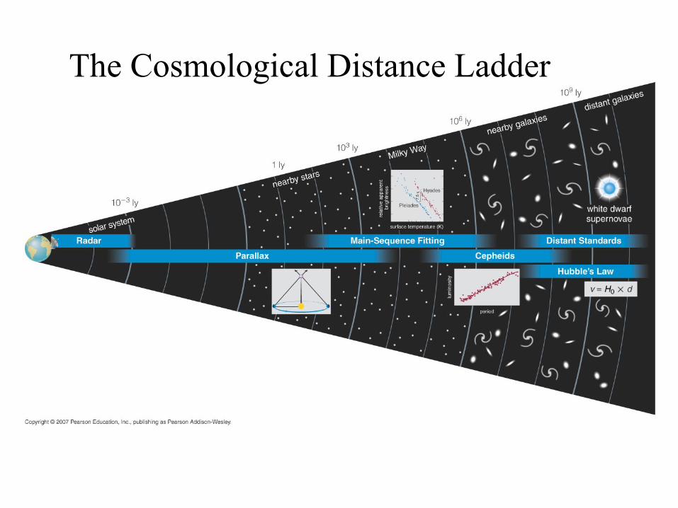
The Cosmological Distance Ladder

The most accurate way to calibrate the length of the Astronomical Unit involves radar measurements of the distances to inner solar system objects, such as Venus and some near-Earth asteroids. Trigonometric parallaxes rely on accurate measurements of stellar positions and a knowledge of the length of the AU.

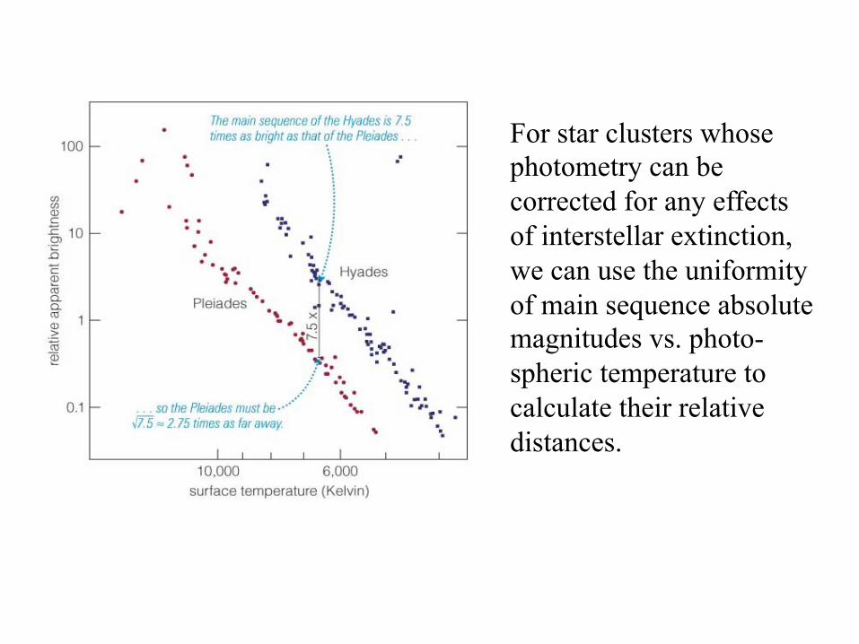
For star clusters whose photometry can be corrected for any effects of interstellar extinction, we can use the uniformity of main sequence absolute magnitudes vs. photo- spheric temperature to calculate their relative distances.

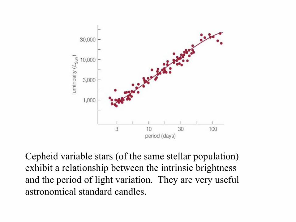
Cepheid variable stars (of the same stellar population) exhibit a relationship between the intrinsic brightness and the period of light variation. They are very useful astronomical standard candles.

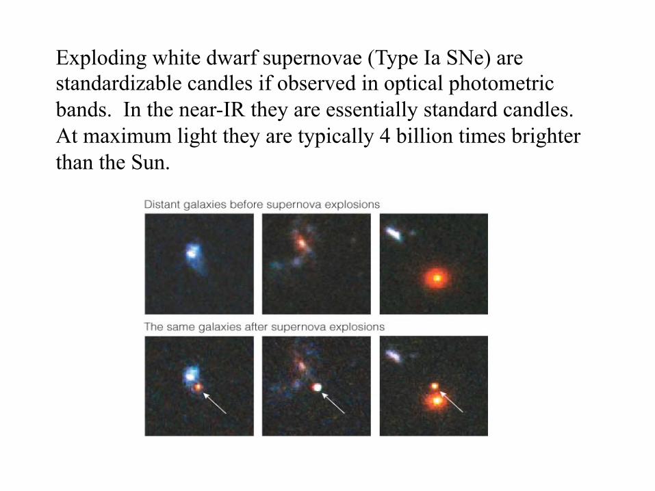
Exploding white dwarf supernovae (Type Ia SNe) are standardizable candles if observed in optical photometric bands. In the near-IR they are essentially standard candles. At maximum light they are typically 4 billion times brighter than the Sun.

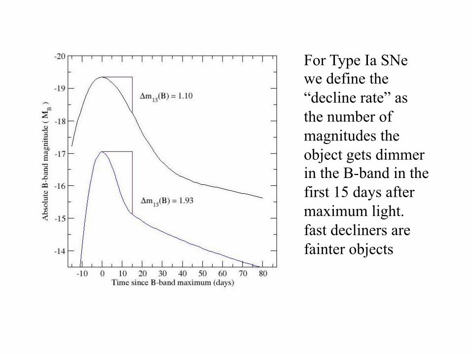
For Type Ia SNe we define the “decline rate” as the number of magnitudes the object gets dimmer in the B-band in the first 15 days after maximum light. fast decliners are fainter objects

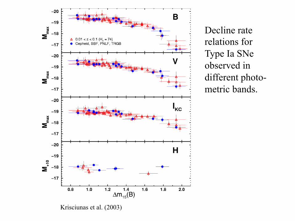
Krisciunas et al. (2003)

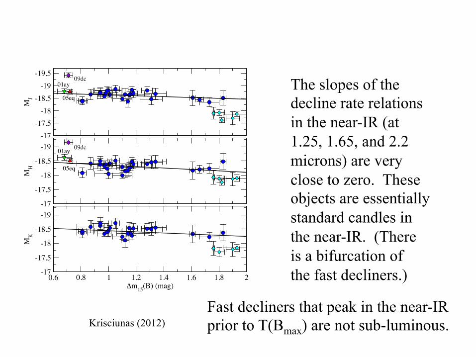
Decline rate relations for Type Ia SNe observed in different photo- metric bands.

-19.5

-19

-18.5

-18

-17.5

-17

MJ

-19

-18.5

-18

-17.5

-17

MH

0.6 0.8 1 1.2 1.4 1.6 1.8 2!m

15(B) (mag)

-19

-18.5

-18

-17.5

-17

MK

05eq

01ay

05eq

01ay

09dc

09dc

The slopes of the decline rate relations in the near-IR (at 1.25, 1.65, and 2.2 microns) are very close to zero. These objects are essentially standard candles in the near-IR. (There is a bifurcation of the fast decliners.)

Krisciunas (2012) Fast decliners that peak in the near-IR prior to T(Bmax) are not sub-luminous.

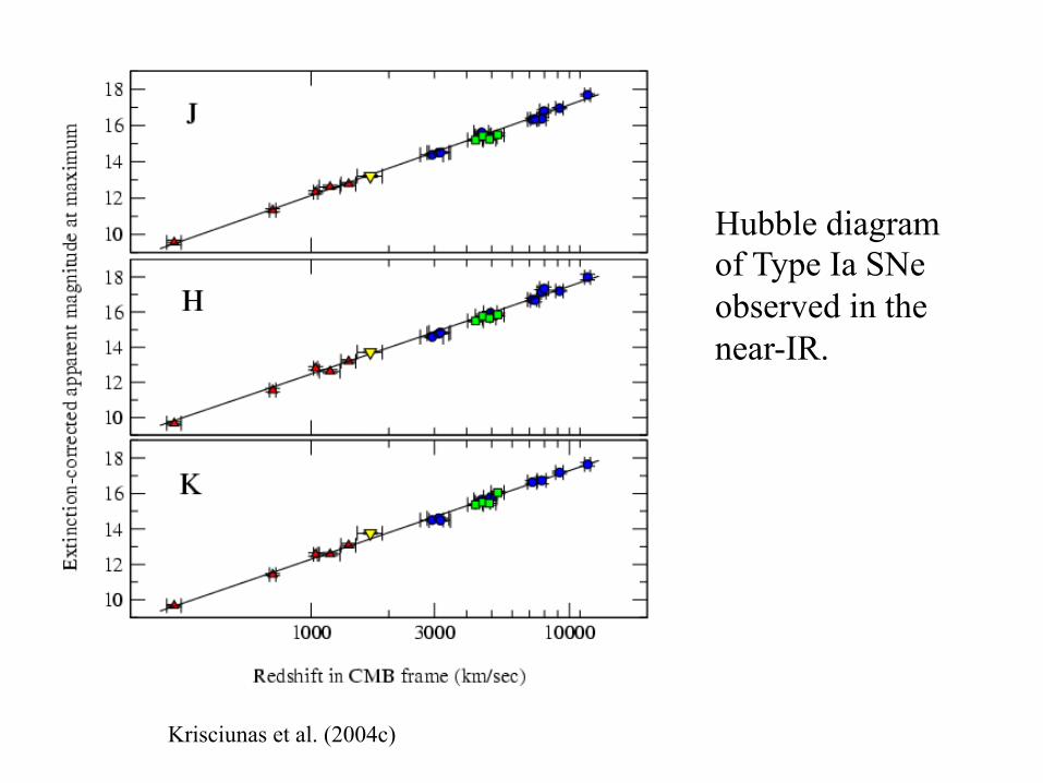
Krisciunas et al. (2004c)

Hubble diagram of Type Ia SNe observed in the near-IR.

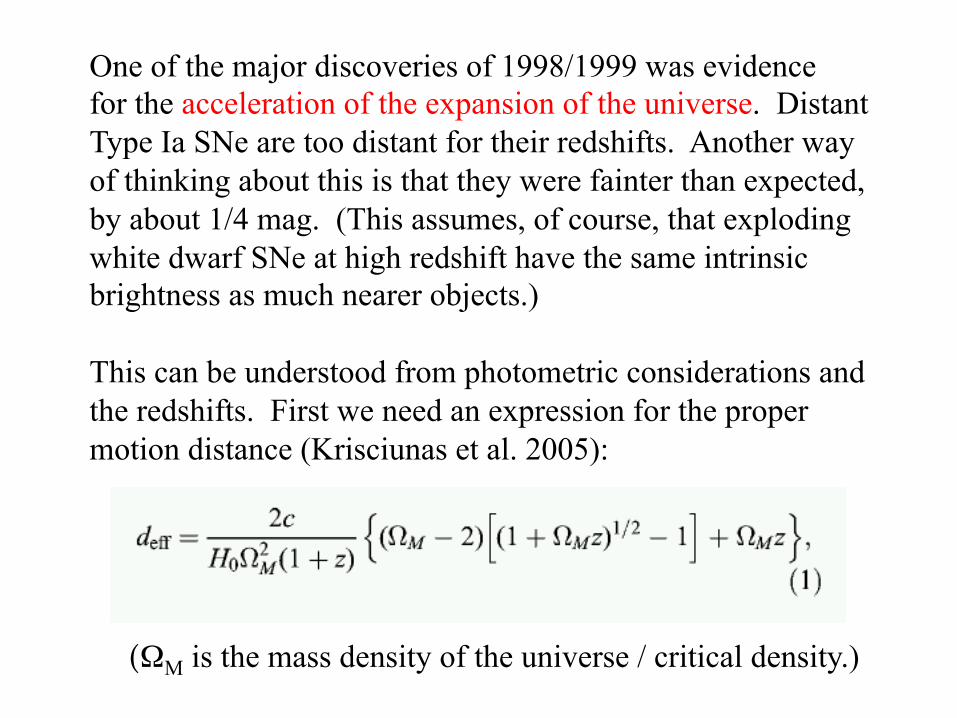
One of the major discoveries of 1998/1999 was evidence for the acceleration of the expansion of the universe. Distant Type Ia SNe are too distant for their redshifts. Another way of thinking about this is that they were fainter than expected, by about 1/4 mag. (This assumes, of course, that exploding white dwarf SNe at high redshift have the same intrinsic brightness as much nearer objects.) This can be understood from photometric considerations and the redshifts. First we need an expression for the proper motion distance (Krisciunas et al. 2005):

(ΩM is the mass density of the universe / critical density.)

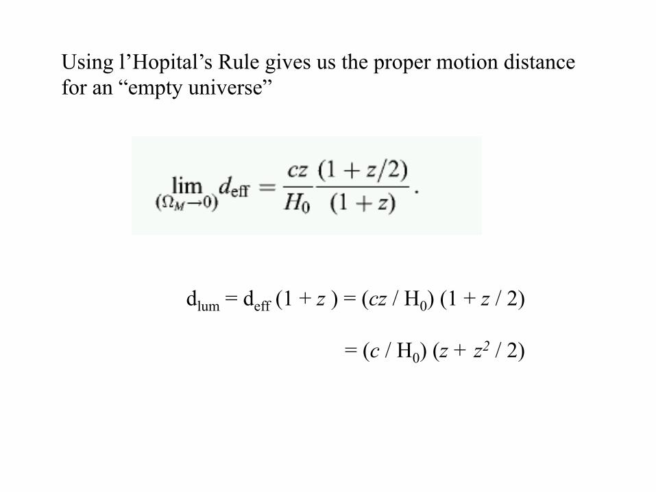
dlum = deff (1 + z ) = (cz / H0) (1 + z / 2) = (c / H0) (z + z2 / 2)

Using l’Hopital’s Rule gives us the proper motion distance for an “empty universe”

For small redshifts (z << 1) the z2 term is negligible and d = cz / H0 . And since z = v/c at small redshift, we get back Hubble’s Law: v = H0 d . Using multi-band observations of Type Ia SNe we can correct the photometry for dimming and reddening effects of interstellar dust. If we have the extinction- corrected magnitude (m) and an estimate of the absolute magnitude (M) from the decline rate, then (m – M) gives us an estimate of the luminosity distance. From the redshift we get another estimate of distance. Further analysis leads to evidence for Dark Energy.

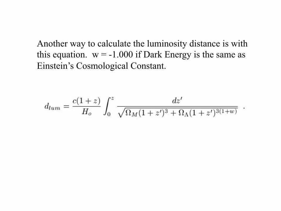
Another way to calculate the luminosity distance is with this equation. w = -1.000 if Dark Energy is the same as Einstein’s Cosmological Constant.

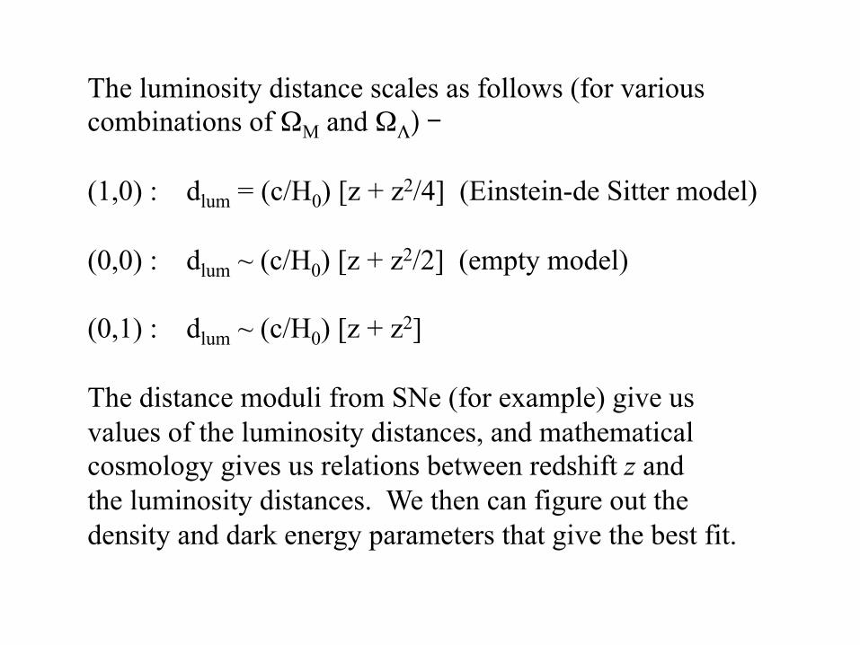
The luminosity distance scales as follows (for various combinations of ΩM and ΩΛ) - (1,0) : dlum = (c/H0) [z + z2/4] (Einstein-de Sitter model) (0,0) : dlum ~ (c/H0) [z + z2/2] (empty model) (0,1) : dlum ~ (c/H0) [z + z2] The distance moduli from SNe (for example) give us values of the luminosity distances, and mathematical cosmology gives us relations between redshift z and the luminosity distances. We then can figure out the density and dark energy parameters that give the best fit.

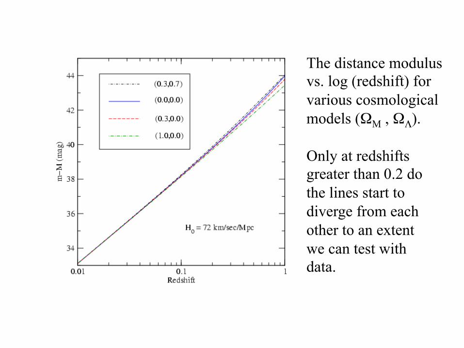
The distance modulus vs. log (redshift) for various cosmological models (ΩM , ΩΛ). Only at redshifts greater than 0.2 do the lines start to diverge from each other to an extent we can test with data.

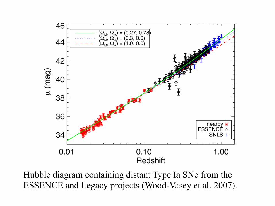
Hubble diagram containing distant Type Ia SNe from the ESSENCE and Legacy projects (Wood-Vasey et al. 2007).

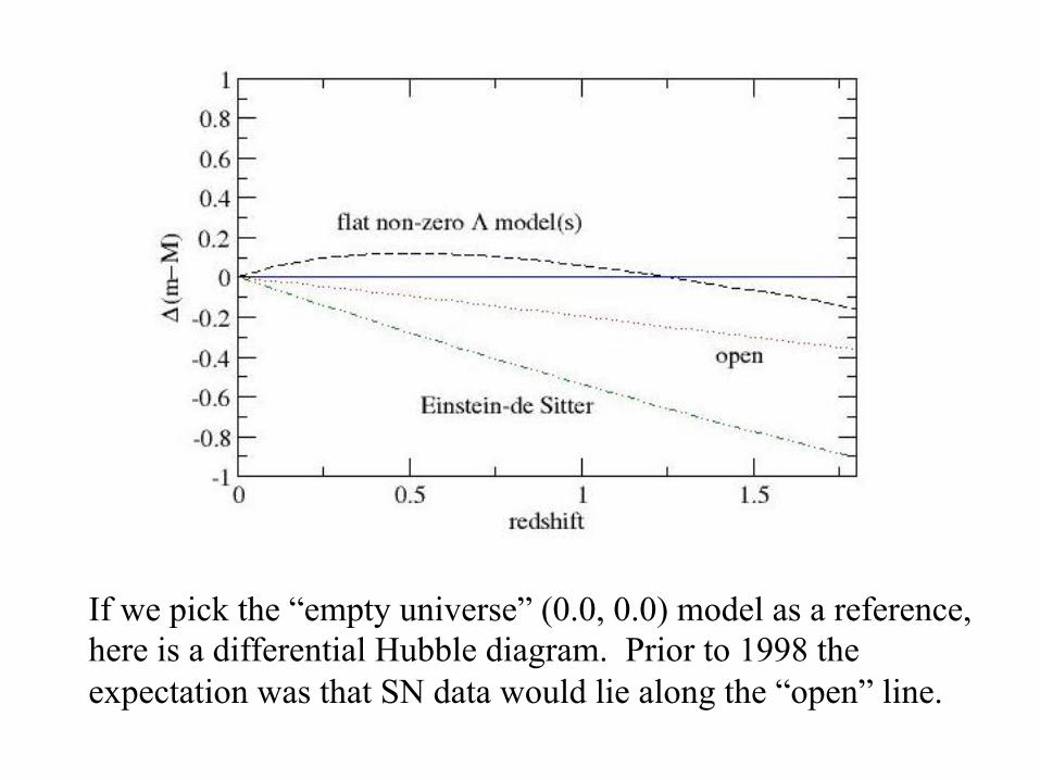
If we pick the “empty universe” (0.0, 0.0) model as a reference, here is a differential Hubble diagram. Prior to 1998 the expectation was that SN data would lie along the “open” line.

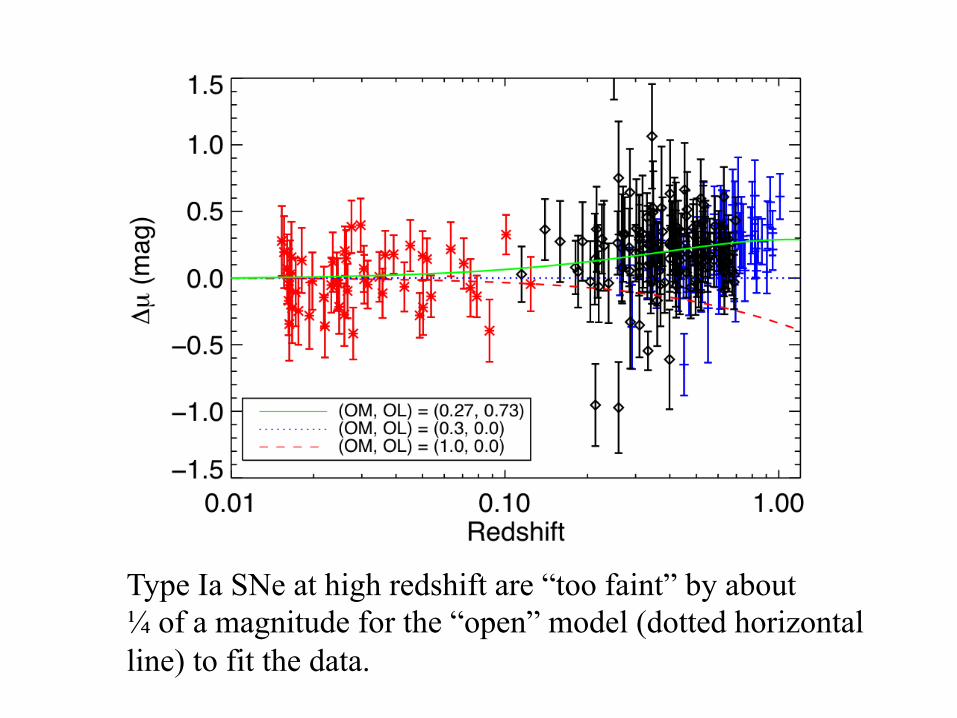
Type Ia SNe at high redshift are “too faint” by about ¼ of a magnitude for the “open” model (dotted horizontal line) to fit the data.

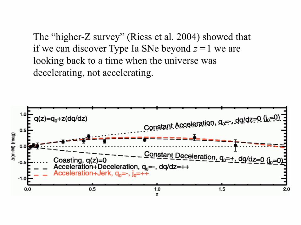
The “higher-Z survey” (Riess et al. 2004) showed that if we can discover Type Ia SNe beyond z =1 we are looking back to a time when the universe was decelerating, not accelerating.