Some Improved Tests for Multivariate One-Sided Hypotheses*

Michael D. Perlman1 and Lang Wu2

1Department of Statistics, University of Washington, Seattle, WA 98195, USA

Email: michael@ms.washington.edu

and

2Department of Statistics, University of British Columbia, Vancouver, B.C., V6T 1Z2, Canada

Email: lang@stat.ubc.ca

July, 2004

Abstract

Multivariate one-sided hypothesis-testing problems are very common in clinical trials with

multiple endpoints. The likelihood ratio test (LRT) and union-intersection test (UIT) are widely

used for testing such problems. It is argued that, for many important multivariate one-sided

testing problems, the LRT and UIT fail to adapt to the presence of subregions of varying dimen-

sionalities on the boundary of the null parameter space and thus give undesirable results. Several

improved tests are proposed that do adapt to the varying dimensionalities and hence re ect the

evidence provided by the data more accurately than the LRT and UIT. Moreover, the proposed

tests are often less biased and more powerful than the LRT and UIT.

Key Words: One-sided hypothesis, multiple endpoints, likelihood ratio test, union-intersection

test, p-value.

*Research supported in part by U. S. National Science Foundation Grant No. DMS00-71818 and

Canada Natural Sciences and Engineering Research Council grant No. 22R80742.

1

1 Introduction

One-sided tests for comparing multivariate treatment e�ects have received much attention in the

literature (e.g., O'Brien (1984), Bloch et al. (2001), Tamhane and Logan (2004)). These tests are

useful in clinical trials with multiple endpoints. For example, in clinical trials, treatment e�ects are

often measured by both eÆcacy and toxicity, which may be measured by more than one response

variable. In principle, a treatment is usually deemed better than its competitor if all components

of its mean responses are larger (say). In some practical situations, it may be diÆcult to show that

each component is better { instead the treatment will be preferred if at least one of its response

components is greater than that of the competitor and if none of the remaining components are

signi�cantly worse (Bloch et al. 2001).

Suppose that there are two treatment groups, with ni subjects in group i; i = 1; 2: Let �Yij

be the sample mean for the jth response to treatment i, and let �ij be the population mean of the

jth response to treatment i, j = 1; : : : ; p. Without loss of generality, we assume that larger values

of �ij correspond to better responses. Let Xj = (n�11 + n�12 )�1=2( �Y1j � �Y2j); �j = �1j � �2j ;X =

(X1; : : : ;Xp); and � = (�1; : : : ; �p). We assume that X follows a multivariate normal distribution

with mean vector � and unknown covariance matrix �. We �rst focus on testing that at least one

response for the �rst treatment is better than the corresponding response of the second, formally,

testing

H0 : maxf�j j 1 � j � pg � 0; vs. H1 : maxf�j j 1 � j � pg > 0; (1)

Testing problem (1) is perhaps more common in selection and ranking problem for �nding the

largest element of several normal means (Gupta 1965; Hsu 1996, Shimodaira and Hasegawa 1999;

Shimodaira 2000). In such problems, we often want to construct the con�dence set for the index of

the largest mean by simultaneously testing several normal mean di�erences, which is closely related

to multiple comparisons with the unknown best (Hsu 1996; Shimodaira 2000). In Section 5, we

2

present such an application in �nding true phylogenies.

For multi-parameter order-restricted hypothesis testing problems such as (1), the standard

Hotelling T 2 test is undesirable since it fails to incorporate the restrictions on the null and alterna-

tive parameter spaces. Under the normality assumption, the likelihood ratio test (LRT) has been

proposed for testing (1), cf. Perlman (1969), Robertson et al. (1988). Since the null space in (1) can

be expressed as an intersection of halfspaces, a reasonable alternative test is the union-intersection

test (UIT). Recently, however, Perlman and Wu [PW] (2002) note that both the LRT and UIT

may exhibit anomalous behavior for testing problems such as (1), since they are unable to adapt to

the di�ering dimensionalities of the boundary of H0 (the nonpositive orthant in Rp). For the case

of known �, [PW] (2002) propose a new test for testing (1) which better adapts to these varying

dimensionalities and which they deem preferable to the LRT and UIT.

In this paper the new test of [PW] (2002) is both improved and extended to more general and

realistic multivariate one-sided testing problems. The anomalies of the LRT and UIT for (1) are

reviewed in Section 2. In x3.1 improvements of the new test of [PW] (2002) are o�ered when � is

assumed known, then extended to the general case of unknown � in x3.3. In x3.5 these ideas are

extended further to a possibly more realistic and practical version of (1), �rst proposed by Bloch al.

(2001) and studied in [PW] (2004). In Section 4 these ideas are then applied to the well-known and

important problem of testing the simple-order restriction. Two real data examples are presented in

Section 5 to illustrate the new tests.

2 Anomalies of the LRT and UIT for (1)

The testing problem (1) can be expressed as that of testing

H0 : � 2 N p vs: H1 : � 2 RpnN p; (2)

3

where N p � f(�1; : : : ; �p) : �1 � 0; : : : ; �p � 0g is the nonpositive orthant in Rp. Here we review

the anomalies of the LRT and UIT for testing (1) � (2) when � is known, say � = I for simplicity.

The size � LRT for (2) (cf. Robertson et al. (1988, x2.2, 2.3)) accepts H0 i�

kX �N pk2 � (X+1 )

2 + � � �+ (X+p )

2 � a2p;�; (3)

where X+i � max(0;Xi) and a2p;� > 0 is the unique solution to the equation

� =pX

i=1

2�p p

i

!P (�2i > a2p;�): (4)

Next, because H0 can also be written as H0 : \pi=1H0i, where H0i : �i � 0, the size � UIT accepts

H0 i�

max(X1; : : : ; Xp) � up;�; (5)

where up;� = ��1( pp1� � ). It is straightforward to verify that up;� < ap;�. (See Figure 1.)

Although the LRT and UIT have been popular for testing (1) � (2), [PW] (2002) argued that

both tests may yield inappropriate inferences, especially for large p. For example, suppose that p = 2

and � = 0:05. It can be shown that the size � LRT rejects H0 if [(X+1 )

2+(X+2 )

2]1=2 > 2:05, and the

size � UIT rejects H0 if max(X1;X2) > 1:95. Now, suppose that we observe X� = (1:8;�10). Then,

neither the LRT nor the UIT reject H0 (see Figure 1). However, if we consider testing H01 : �1 � 0

vs H11 : �1 > 0, we see that H01 is rejected (note that z� := ��1(:95) = 1:64), and therefore H0

should also be rejected since H0 � H01.

This anomalous behavior becomes more emphatic as p increases. Suppose that X� is a sample

point such that (i) X�i � z� and (ii) maxj 6=iX

�j ! �1, where 1 � i � p is �xed. Since up;� !1

as p ! 1, the size � UIT fails to reject H0. However, (ii) strongly indicates that maxj 6=i �j � 0,

so the null hypothesis in (1) reduces to H0;i : �i � 0, while (i) indicates that H0;i should be

strongly rejected. Since X1; : : : ;Xp are independent with standard deviation 1, the observation X�

therefore provides strong evidence against H0i thus also against H0 (since H0 � H0i), so the UIT

4

exhibits contradictory behavior. Since ap;� > up;� ! 1 as p ! 1, the LRT exhibits similarly

contradictory behavior. In fact, for a sequence of alternatives (�1; : : : ; �p) with �1 arbitrarily large

but maxi6=1�j ! �1 as p ! 1, the powers of the LRT and UIT approach zero, but for such

alternatives, any appropriate test procedure should have reasonable power to reject H0. This anti-

evidence property of the LRT and UIT renders these two tests undesirable for problem (1) � (2)

with � known.

This contradictory behavior is explained as follows. The orthant N p is a convex polyhedral

cone whose boundary consists of a union of faces of dimensions 0 (the origin), 1; : : : ; p � 1. Thus

the boundary of H0 can be thought of as a union of statistical models of varying dimensionalities.

Because the least favorable distribution occurs at � = 0, the LRT and UIT thus determine their

critical values with reference to the model (face) of lowest dimension and are therefore biased in favor

of the models (faces) of highest dimension, sometimes failing to reject these models (and therefore

failing to reject H0) despite strong evidence to the contrary (for example, as provided by X�). We

conclude that the contradictory behavior of the LRT and UIT is due to their inability to adapt to

the di�erent dimensions of the faces of N p. Such contradictory behavior of the LRT and UIT also

occur in other multi-parameter testing problems where the null parameter space or its boundary

consists of subregions of varying dimensionalities (cf. [PW] (2002, 2004)).

3 The New Tests for (1) � (2)

3.1 The case � known (� = I)

Tests more appropriate for (1) � (2) than the LRT and UIT should adapt to the varying dimen-

sionalities in the boundary of H0 { in this case, to the dimension of the face of N p closest to the

sample point X. Shimodaira (2000) proposed such a test based on bootstrap methods. However,

5

his method is computational intensive, especially when p is large, and is limited to the case where

� is known. For the simple case � = I, [PW] (2002) proposed a new test (see (7) below) for (1) �

(2) that utilizes the p-values associated with the LRTs for testing the individual faces of N p against

H1. Since a p-value is \self-weighting" according to the dimensionality of its null hypothesis, this

new test thus adapts to the varying dimensionalities of the faces.

Let Sp = 2f1;:::;pg n ; denote the collection of all nonempty subsets of f1; : : : ; pg. For each

� 2 Sp, de�ne L� = f� 2 Rp j �i = 0; 8 i 2 �g and F� = L� \ N p. Then L� is a linear subspace

of dimension p� j�j and fF� j � 2 Spg is the family of faces of N p � [�2Sp F�. For � 2 Spn;, let

T� � T�(X) be a statistic appropriate for testing

H0;� : � 2 F� vs: H1 : � 2 RpnN p (6)

and let ��(T�) be the associated p-value. Then the test that accepts H0 i�

max�2Spn;

��(T�(X)) � � (7)

is expected to be an approximately size � test for (1) � (2). This test uses the individual p-values

�� to adapt to the varying dimensionalities of the faces F�.

Because it may be diÆcult to choose appropriate statistics T� and calculate the correspond-

ing p-values ��, [PW] (2002) instead proposed an explicit and computationally simpler test (here

denoted by PW1) that approximates the test (7). Test PW1 accepts H0 i�

(1� 1N p(X))Xi2�

X2i � ~a2j�j;� and max

i=2�Xi � 0 (8)

for at least one � 2 Spn; (see Figure 1) , where

~a2k;� := �G�1k

��

1� 2�k

�; k = 1; : : : ; p; (9)

and Gk � 1� �Gk is the cdf of the �2k distribution. Note that

Pi2� X2

i is the appropriate �2k statistic

for testing � 2 L� vs. � =2 L�. The divisor 1 � 2�k in (9) renders this statistic appropriate for

testing � 2 L� vs. maxf�i j i 2 �g > 0.

6

The test PW1 in (8) better adapts to the varying dimensionalities of the faces F� of N p and so

reduces the undesirable behavior of the LRT and UIT. Simulation results in [PW] (2002) show that

PW1 is approximately size � for (1) � (2), is more nearly similar on the boundary of H0, and is more

nearly unbiased than the LRT and the UIT. Moreover, PW1 has better overall power performance

than the LRT and the UIT. Note, however, that as argued by [PW] (1999), our preference for PW1

is based not mainly on consideration of power and unbiasedness but rather on the fact that it better

re ects the evidence that the data provides regarding the competing hypotheses in (1).

We now propose two modi�cations of PW1 that re ect this evidence even more accurately

and also improve its power and unbiasedness properties. The �rst modi�ed test, denoted as PW2,

has acceptance region obtained by replacing ~aj�j;� in (8) by aj�j;� (cf. (3)). This is motivated by

the fact that it is aj�j;�, not ~aj�j;�, that is the critical value for the LRT for testing the individual

face F�. Another alternative test, denoted by PW3, replaces ~aj�j;� in (8) by the average lj�j;� �

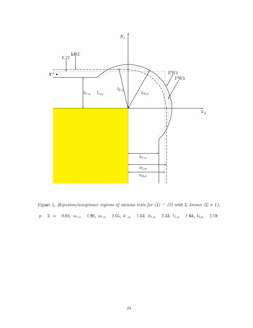
(~aj�j;� + aj�j;�)=2. Figure 1 shows the acceptance regions of the LRT, UIT, PW1, and PW3 tests.

(To avoid overcrowding, PW2, which is qualitatively similar to PW1 and PW3, is not depicted.)

Figure 1 here: rejection regions of the LRT, UIT, PW1, and PW3.

It is seen from Figure 1 that, unlike the LRT and UIT, the new tests PW1, PW2, and PW3

do not have monotone acceptance regions. Since H0 is composite, however, monotonicity is not a

natural requirement for the testing problem (1) � (2). For example, it is easy to construct prior

distributions for which the corresponding Bayes (therefore admissible) tests are not monotone, so

the class of monotone tests does not form a complete class.

3.2 Simulations for the case � known (� = I).

The newly proposed tests PW2 and PW3 are compared to the LRT, UIT, and PW1 via simulations

for dimensions p = 2; 5 and various representative choices of the mean vector �. In all simulations

7

throughout the article, we choose the nominal size � = 0:05(= 5%), sample sizes n1 = n2 = 40,

and 5000 iterations in each case. Table 1 shows the type I error rates and powers for the �ve tests.

The new test PW2 appears to be slightly too liberal in that its type I error rate sometimes exceeds

the nominal level � = 0:05, so is eliminated from contention. Of the remaining four tests, PW3

is more nearly similar (hence more nearly unbiased) on the boundary of H0 at its faces of higher

dimension, while the UIT appears more nearly similar at the faces of lowest dimension but the

di�erences here are not as pronounced. PW3 is more nearly similar than PW1 in all cases, both

tests better adapt to the varying dimensionalities of the boundary of H0 than UIT/LRT (e.g., for

boundary points far from the origin such as � = (�5; 0) or � = (�24; 0), the type I error rates for

PW3/PW1 are much closer to the nominal level � = 5% than for UIT/LRT). Furthermore, the

power of PW3 is greater than that of the others, except in the central region of the positive orthant

of the alternative parameter space H1 where the power of the LRT is somewhat greater. (This

conforms to the behavior to be expected in light of the nature of the acceptance regions in Figure

1.) PW3 is more powerful than PW1 in all cases, and both PW3 and PW1 can be substantially

more powerful than LRT/UIT in many cases (see, e.g., when � = (�54; 1)). Therefore, we conclude

that the new test PW3 gives better results than all other tests, so PW3 is our recommended choice

for testing (1) � (2) when � = I.

3.3 The general case: � unknown

In this section we extend the results in the previous section to the general and more realistic case

where the covariance matrix � is completely unknown. Let �̂ denote the pooled sample covariance

matrix and n = n1 + n2 � 2, so S � n�̂ has the Wishart distribution Wp(�; n) (assume that

n1 + n2 � p+ 2). From Perlman (1969), the size � LRT for (1) � (2) with � unknown accepts H0

8

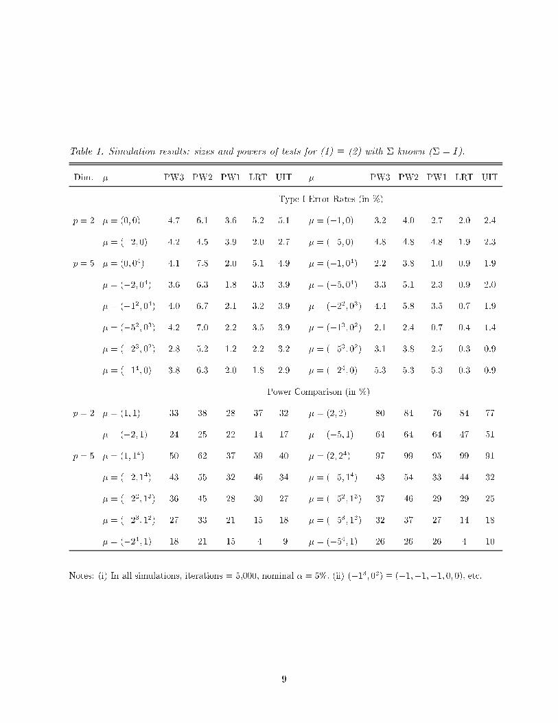
Table 1. Simulation results: sizes and powers of tests for (1) � (2) with � known (� = I).

Dim. � PW3 PW2 PW1 LRT UIT � PW3 PW2 PW1 LRT UIT

Type I Error Rates (in %)

p = 2 � = (0; 0) 4.7 6.1 3.6 5.2 5.1 � = (�1; 0) 3.2 4.0 2.7 2.0 2.4

� = (�2; 0) 4.2 4.5 3.9 2.0 2.7 � = (�5; 0) 4.8 4.8 4.8 1.9 2.3

p = 5 � = (0; 04) 4.1 7.8 2.0 5.1 4.9 � = (�1; 04) 2.2 3.8 1.0 0.9 1.9

� = (�2; 04) 3.6 6.3 1.8 3.3 3.9 � = (�5; 04) 3.3 5.1 2.3 0.9 2.0

� = (�12; 03) 4.0 6.7 2.1 3.2 3.9 � = (�22; 03) 4.4 5.8 3.5 0.7 1.9

� = (�52; 03) 4.2 7.0 2.2 3.5 3.9 � = (�13; 02) 2.1 2.4 0.7 0.4 1.4

� = (�23; 02) 2.8 5.2 1.2 2.2 3.2 � = (�53; 02) 3.1 3.8 2.5 0.3 0.9

� = (�14; 0) 3.8 6.3 2.0 1.8 2.9 � = (�24; 0) 5.3 5.3 5.3 0.3 0.9

Power Comparison (in %)

p = 2 � = (1; 1) 33 38 28 37 32 � = (2; 2) 80 84 76 84 77

� = (�2; 1) 24 25 22 14 17 � = (�5; 1) 64 64 64 47 51

p = 5 � = (1; 14) 50 62 37 59 40 � = (2; 24) 97 99 95 99 91

� = (�2; 14) 43 55 32 46 34 � = (�5; 14) 43 54 33 44 32

� = (�22; 13) 36 45 28 30 27 � = (�52; 13) 37 46 29 29 25

� = (�23; 12) 27 33 21 15 18 � = (�53; 12) 32 37 27 14 18

� = (�24; 1) 18 21 15 4 9 � = (�54; 1) 26 26 26 4 10

Notes: (i) In all simulations, iterations = 5,000, nominal � = 5%: (ii) (�13; 02) � (�1;�1;�1; 0; 0), etc.

9

i�

kX �N pk2S � kX � �S(X;N p)k2S � a�p;�; (10)

where kxk2S � xtS�1x is the Euclidean norm determined by S, �S(X;N p) is the projection of X

onto N p with respect to this norm, and a�p;� is the critical value of the size � LRT for H0 determined

by the equation

� =1

2Pr

"�2p�1

�2n1+n2�p> a�p;�

#+1

2Pr

"�2p

�2n1+n2�p�1> a�p;�

#(11)

� sup�2N p;�>0

Pr�;�[ kX �N pk2S > a�p;�]: (12)

Perlman (1969) showed that �S(X;N p) is the MLE of � under H0 : � 2 N p with � unknown.

Tang (1994) has tabulated some values of a�p;�. The values of a�p;� can also be determined by

numerical methods. The LR statistic can be computed by a program for minimizing linear inequality-

constrained Mahalanobis distance (Wollan and Dykstra (1987)).

The UIT for (1) � (2) with � unknown accepts H0 i�

max (t1; : : : ; tp) � vp;�; (13)

where ti = Xipsii

and s11; : : : ; spp are the diagonal elements of S. Under H0 the distribution of

max (t1; : : : ; tp) is stochastically largest when � = 0, so the critical value vp;� may be approximated

from the Bonferroni inequality as follows: vp;� � tn;�=p, the upper (�=p)-quantile of the Student

t-distribution with n degrees of freedom (cf. Tamhane and Logan (2004)).

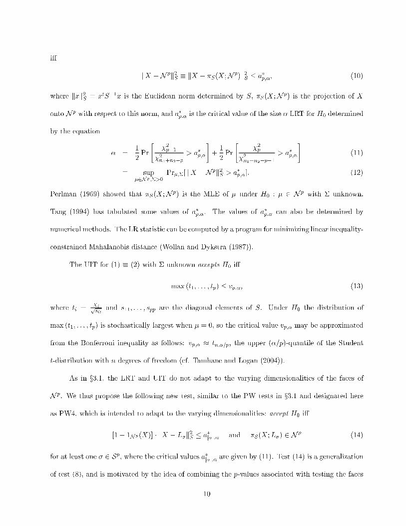
As in x3.1, the LRT and UIT do not adapt to the varying dimensionalities of the faces of

N p. We thus propose the following new test, similar to the PW tests in x3.1 and designated here

as PW4, which is intended to adapt to the varying dimensionalities: accept H0 i�

[1� 1N p(X)] � kX � L�k2S � a�j�j;� and �S(X;L�) 2 N p (14)

for at least one � 2 Sp, where the critical values a�j�j;� are given by (11). Test (14) is a generalization

of test (8), and is motivated by the idea of combining the p-values associated with testing the faces

10

of N p individually, as in Perlman and Wu (2002). Thus, the new test should be preferable to the

LRT and UIT, as shown next.

3.4 Simulations for the general case: � unknown.

In this section we compare the new test PW4 (14) with the LRT and UIT via simulations. For

dimensions p = 2 and p = 5, the size and power of the tests are simulated for various representative

choices of the mean vector � and four covariance matrices �1; : : : ;�4. Each �i is an intraclass

correlation matrix with all diagonal elements = 1 and all o�-diagonal elements = �i, with �1 = 0,

�2 = 0:4, �3 = 0:8, �4 = �0:2. In particular, �1 = I, the identity matrix. The sample sizes in all

simulations are n1 = n2 = 40 (results for sample sizes n1 = n2 = 20 were similar) and the iteration

number is 5000, as noted earlier.

Simulated values of Type I error rates and powers for the three tests are given in Table 2.

The new test PW4 in (14) more nearly attains the nominal level � = 5% while the LRT and UIT

can be very conservative in some cases (e.g., when � = (�14; 0), etc). PW4 appears to better adapt

to the dimensionality of the faces of H0 (e.g., for boundary points far from the origin 0, the type

I errors for PW4 are much closer to the nominal level � than for UIT/LRT), and is more nearly

similar on the boundary (so less biased) than the LRT and UIT. Also, PW4 is more powerful than

the LRT and UIT in most cases, except perhaps in the central region of the positive orthant of the

alternative parameter space H1 when the correlation is negative. The power advantage of PW4 over

LRT and UIT can be substantial (see, e.g., when � = (�14; 0:5), etc). The performance of LRT

and UIT seems to be mixed: neither test dominates the other. It appears that the UIT adapts the

dimensionality slightly better than the LRT, but both are usually worse than the new test PW4.

We conclude that PW4 is the test of preference.

11

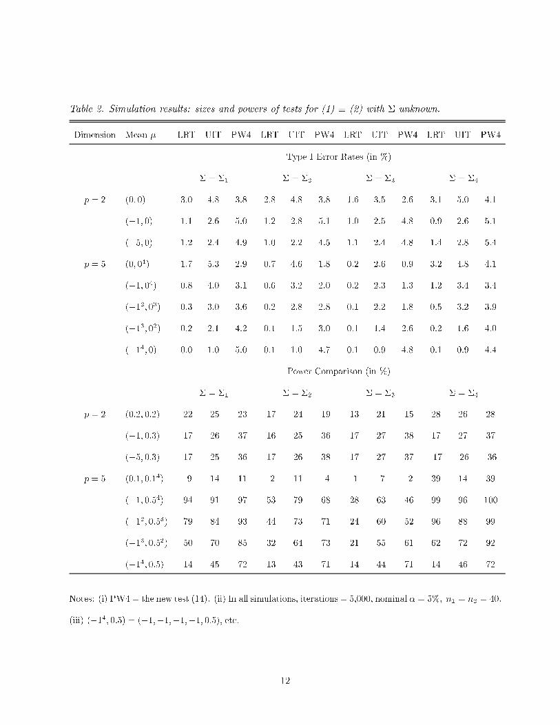
Table 2. Simulation results: sizes and powers of tests for (1) � (2) with � unknown.

Dimension Mean � LRT UIT PW4 LRT UIT PW4 LRT UIT PW4 LRT UIT PW4

Type I Error Rates (in %)

� = �1 � = �2 � = �3 � = �4

p = 2 (0; 0) 3.0 4.8 3.8 2.8 4.8 3.8 1.6 3.5 2.6 3.1 5.0 4.1

(�1; 0) 1.1 2.6 5.0 1.2 2.8 5.1 1.0 2.5 4.8 0.9 2.6 5.1

(�5; 0) 1.2 2.4 4.9 1.0 2.2 4.5 1.1 2.4 4.8 1.4 2.8 5.4

p = 5 (0; 04) 1.7 5.3 2.9 0.7 4.6 1.8 0.2 2.6 0.9 3.2 4.8 4.1

(�1; 04) 0.8 4.0 3.1 0.6 3.2 2.0 0.2 2.3 1.3 1.2 3.4 3.4

(�12; 03) 0.3 3.0 3.6 0.2 2.8 2.8 0.1 2.2 1.8 0.5 3.2 3.9

(�13; 02) 0.2 2.1 4.2 0.1 1.5 3.0 0.1 1.4 2.6 0.2 1.6 4.0

(�14; 0) 0.0 1.0 5.0 0.1 1.0 4.7 0.1 0.9 4.8 0.1 0.9 4.4

Power Comparison (in %)

� = �1 � = �2 � = �3 � = �4

p = 2 (0:2; 0:2) 22 25 23 17 24 19 13 21 15 28 26 28

(�1; 0:3) 17 26 37 16 25 36 17 27 38 17 27 37

(�5; 0:3) 17 25 36 17 26 38 17 27 37 17 26 36

p = 5 (0:1; 0:14) 9 14 11 2 11 4 1 7 2 39 14 39

(�1; 0:54) 94 91 97 53 79 68 28 63 46 99 96 100

(�12; 0:53) 79 84 93 44 73 71 24 60 52 96 88 99

(�13; 0:52) 50 70 85 32 64 73 21 55 61 62 72 92

(�14; 0:5) 14 45 72 13 43 71 14 44 71 14 46 72

Notes: (i) PW4 = the new test (14). (ii) In all simulations, iterations = 5,000, nominal � = 5%; n1 = n2 = 40:

(iii) (�14; 0:5) = (�1;�1;�1;�1; 0:5), etc.

12

3.5 A related testing problem

Testing problem (1) � (2) is formulated to determine whether or not at least one endpoint in

treatment 1 (say) is signi�cantly superior than the corresponding endpoint in treatment 2. As

noted in Section 1, however, Bloch et al. (2001) argue that sometimes it is more practical to

assert that treatment 1 is preferred if it is superior for at least one of the endpoints and biologically

\noninferior" for the remaining endpoints. This leads to the following reformulated testing problem:

test

H 00 : � 2 �0 �

�max1�j�p

�j � 0

�[�max1�j�p

�j > 0 and �j � ��j for some j�; (15)

versus H 01 : not H

00, where �j 's are pre-speci�ed positive numbers. Again assume that � is unknown.

Bloch et al. (2001) noted that H 00 is a union of H0 : � 2 N p and H

(j)0 : �j � ��j; j = 1; : : : ; p,

so an intersection-union test (IUT) is appropriate for (15). They combined the Hotelling T 2-test for

H�0 : � = 0 with the usual t-tests for H

(j)0 ; j = 1; : : : ; p, thus obtaining the following approximate

size � test: reject H 00 i�

T 2 � b�t�̂�1b� > c�; and b�j + �j=s1=2jj > u� for all j = 1; � � � ; p; (16)

where u� = tn;�, the upper �-quantile of the tn-distribution, and c� is the size � critical value for

the Hotelling T 2 statistic.

Because the Hotelling T 2-test for H�0 is not designed to test the one-sided hypothesisH0, [PW]

(2004) asserted that a more appropriate test, here designated as PW5, is obtained by replacing T 2 by

the LRT statistic for testing H0 in (1) � (2) (� unknown), which better re ects its one-sided form.

As noted above, however, this LRT does not adapt to the varying dimensionalities in the boundary

of H0. Therefore, here we propose an even more appropriate IUT for (15) with � unknown, obtained

by replacing the T 2-test in (16) by the new test (14). The resulting size � IUT test, here designated

13

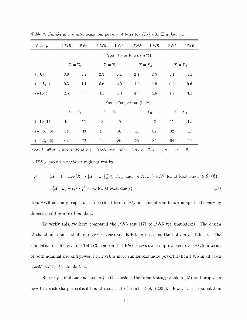
Table 3. Simulation results: sizes and powers of tests for (15) with � unknown.

Mean � PW5 PW6 PW5 PW6 PW5 PW6 PW5 PW6

Type I Error Rates (in %)

� = �1 � = �2 � = �3 � = �4

(0; 0) 3.0 3.9 2.3 3.1 2.1 2.8 3.1 4.1

(�0:5; 0) 0.3 1.1 0.6 2.9 1.2 4.9 0.2 0.6

(�1; 0) 2.5 3.6 4.1 4.8 4.6 4.6 1.7 3.1

Power Comparison (in %)

� = �1 � = �2 � = �3 � = �4

(0:1; 0:1) 10 11 8 9 6 8 11 12

(�0:5; 0:5) 34 49 40 56 44 62 32 44

(�0:2; 0:6) 64 72 64 80 65 85 64 69

Note: In all simulations, iterations = 5,000, nominal � = 5%; p = 2; � = 1; n1 = n2 = 40:

as PW6, has an acceptance region given by

A = fX : [1� 1N p(X)] � kX � L�k2S � a�j�j;� and �S(X;L�) 2 N p for at least one � 2 Spn;g

[fX : b�j + �j=�̂1=2jj � u� for at least one jg: (17)

Test PW6 not only respects the one-sided form of H0 but should also better adapt to the varying

dimensionalities in its boundary.

To verify this, we have compared the PW6 test (17) to PW5 via simulations. The design

of the simulation is similar to earlier ones and is brie y noted at the bottom of Table 3. The

simulation results, given in Table 3, con�rm that PW6 shows some improvement over PW5 in terms

of both nominal size and power, i.e., PW6 is more similar and more powerful than PW5 in all cases

considered in the simulations.

Recently, Tamhane and Logan (2004) consider the same testing problem (15) and propose a

new test with sharper critical bound than that of Bloch et al. (2001). However, their simulation

14

results indicate that PW5 may still be better than their new test. Since [PW] (2004) already

demonstrated that PW5 performs better than the test of Bloch et al. (2001) and Bloch et al.

(2001) showed that their test is better than previous tests in the literature, we conclude that PW6

is the best test among all previously proposed tests for testing (15).

4 Testing the Simple-Order Restriction

4.1 The case � known (� = I)

The anomalous behavior of the LRT and IUT occurs in any multivariate testing problem where the

null parameter space or its boundary is the union of sets of varying dimensionalities, in particular

a polyhedral cone, and, as for the nonpositive orthant cone, new tests that adapt to these dimen-

sionalities may be obtained. Here we focus on the LRT for the well-known problem of testing the

simple-order cone (cf. Robertson et al. 1988, Ch.2).

Let Cp denote the simple-order cone in Rp de�ned by

Cp = f� � (�1; : : : ; �p) 2 Rp j �1 � � � � � �pg; (18)

which is a non-pointed1 acute polyhedral cone with \spine" given by the line f� j �1 = � � � = �pg:

Consider the problem of testing

�H0 : � 2 Cp vs �H1 : � 2 Rp n Cp (19)

based on the data X � (X1; : : : ;Xp) � N(�;�). For the case � known with � = I, the LRT for

(19) accepts �H0 i�

kX � Cpk2 � kX � �(X; Cp)k2 � d2p;�; (20)

1A convex cone C is non-pointed if it contains a nontrivial linear subspace. Its spine L is the maximal such subspace,

and C can be uniquely represented as the product L� ~C, where ~C is the pointed cone obtained by projecting C onto

the orthogonal complement L?.

15

where d2p;� satis�es

� =p�1Xi=1

P (i; p) Pr[�2p�i > d2p;�] (21)

and fP (i; p) j i = 1; : : : ; pg are the level probabilities associated with the LRT statistic for the case

of equal weights { cf. Robertson et al. (1988, pp.69-70, 79-82).

We now propose a new test that combines the p-values associated with the faces of Cp. Let Fp

denote the set of faces of Cp. There is a 1-1 correspondence between Fp and Sp�1 � 2f1;:::;p�1g n ;,

described as follows. Each face F 2 Fp has the form F� � L� \ Cp for some unique � 2 Sp�1,

where L� � Rp is the linear subspace given by L� = f� j �i = �i+1; 8i 2 �g: Conversely, each

� 2 Sp�1 determines a unique face F� . The dimension of both L� and F� is p� j� j. For example, if

p = 5 and F is the face of C5 that spans the linear subspace given by the constraints �1 = �2 and

�3 = �4 = �5, then F = F� where � = f1; 3; 4g and dim(F� ) = 2.

For each � 2 Sp�1, let T� � T� (X) be a statistic appropriate for testing

H0;� : � 2 F� vs: H : � 2 RpnCp (22)

and let p� � p(T� ) be the associated p-value. Then the test (compare to (7)) that accepts �H0 i�

max�2Sp�1

p� � � (23)

will be an approximately size � test for (19). This test uses the individual p-values p� to adapt to

the varying dimensionalities of the faces F� of the polyhedral cone Cp.

Because it may be diÆcult to choose appropriate statistics T� and/or to calculate the corre-

sponding p-values p� , we propose instead the following test, denoted by PW7, which is qualitatively

similar to (23) and somewhat easier to implement: accept �H0 i�

[1� 1Cp(X)] � kX � L�k2 � b2j� j;� and �I(X;L� ) 2 Cp (24)

16

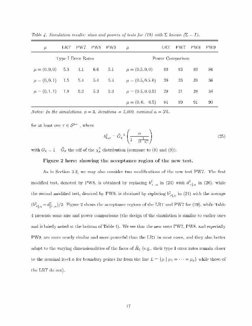
Table 4. Simulation results: sizes and powers of tests for (19) with � known (� = I).

� LRT PW7 PW8 PW9 � LRT PW7 PW8 PW9

Type I Error Rates Power Comparison

� = (0; 0; 0) 5.3 4.1 6.6 5.1 � = (0:5; 0; 0) 89 83 89 86

� = (0; 0; 1) 1.5 5.4 5.4 5.4 � = (0:5; 0:5; 0) 30 33 39 36

� = (0; 1; 1) 1.8 5.3 5.3 5.3 � = (0:5; 0; 0:5) 29 31 38 34

� = (0; 0;�0:5) 84 89 91 90

Notes: In the simulations, p = 3, iterations = 5,000, nominal � = 5%:

for at least one � 2 Sp�1, where

b2k;� � �G�1k

0@ �

1� 1(k+1)!

1A (25)

with Gk � 1� �Gk the cdf of the �2k distribution (compare to (8) and (9)).

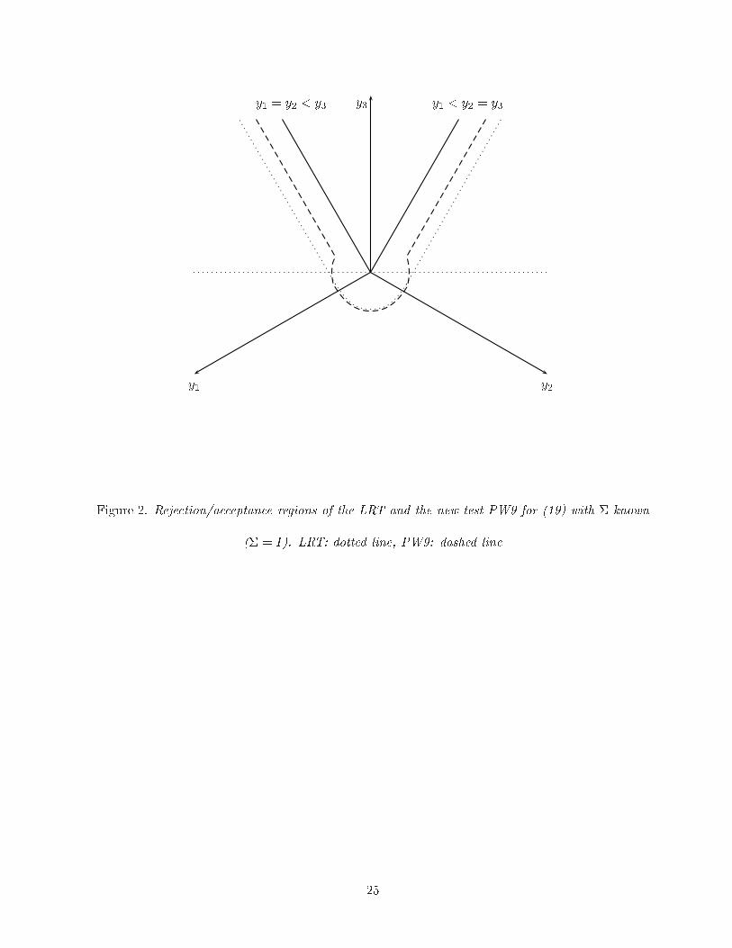
Figure 2 here: showing the acceptance region of the new test.

As in Section 3.2, we may also consider two modi�cations of the new test PW7. The �rst

modi�ed test, denoted by PW8, is obtained by replacing b2j� j;� in (24) with d2j� j;� in (20), while

the second modi�ed test, denoted by PW9, is obtained by replacing b2j� j;� in (24) with the average

(b2j� j;�+ d2j� j;�)=2. Figure 2 shows the acceptance regions of the LRT and PW7 for (19), while Table

4 presents some size and power comparisons (the design of the simulation is similar to earlier ones

and is brie y noted at the bottom of Table 4). We see that the new tests PW7, PW8, and especially

PW9, are more nearly similar and more powerful than the LRT in most cases, and they also better

adapt to the varying dimensionalities of the faces of �H0 (e.g., their type I error rates remain closer

to the nominal level � for boundary points far from the line L � f� j �1 = � � � = �pg while those of

the LRT do not).

17

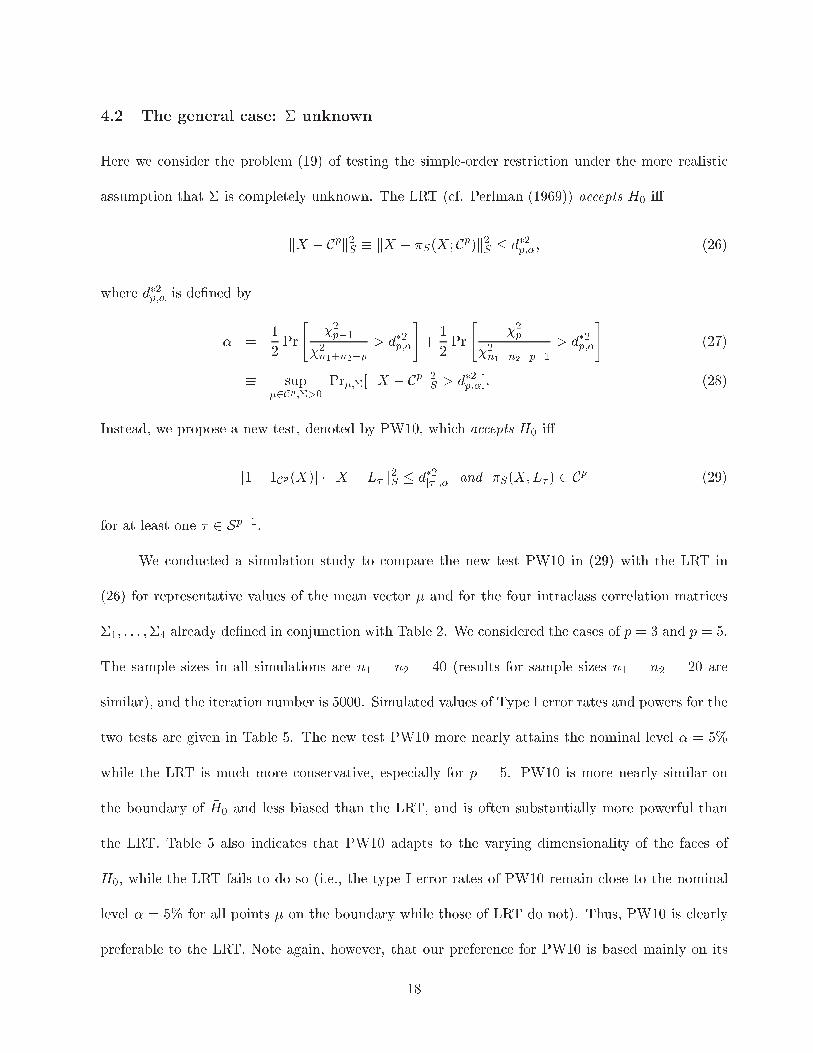
4.2 The general case: � unknown

Here we consider the problem (19) of testing the simple-order restriction under the more realistic

assumption that � is completely unknown. The LRT (cf. Perlman (1969)) accepts �H0 i�

kX � Cpk2S � kX � �S(X; Cp)k2S � d�2p;�; (26)

where d�2p;� is de�ned by

� =1

2Pr

"�2p�1

�2n1+n2�p> d�2p;�

#+1

2Pr

"�2p

�2n1+n2�p�1> d�2p;�

#(27)

� sup�2Cp;�>0

Pr�;�[ kX � Cpk2S > d�2p;�]: (28)

Instead, we propose a new test, denoted by PW10, which accepts �H0 i�

[1� 1Cp(X)] � kX � L�k2S � d�2j� j;� and �S(X;L� ) 2 Cp (29)

for at least one � 2 Sp�1.

We conducted a simulation study to compare the new test PW10 in (29) with the LRT in

(26) for representative values of the mean vector � and for the four intraclass correlation matrices

�1; : : : ;�4 already de�ned in conjunction with Table 2. We considered the cases of p = 3 and p = 5.

The sample sizes in all simulations are n1 = n2 = 40 (results for sample sizes n1 = n2 = 20 are

similar), and the iteration number is 5000. Simulated values of Type I error rates and powers for the

two tests are given in Table 5. The new test PW10 more nearly attains the nominal level � = 5%

while the LRT is much more conservative, especially for p = 5. PW10 is more nearly similar on

the boundary of �H0 and less biased than the LRT, and is often substantially more powerful than

the LRT. Table 5 also indicates that PW10 adapts to the varying dimensionality of the faces of

�H0, while the LRT fails to do so (i.e., the type I error rates of PW10 remain close to the nominal

level � = 5% for all points � on the boundary while those of LRT do not). Thus, PW10 is clearly

preferable to the LRT. Note again, however, that our preference for PW10 is based mainly on its

18

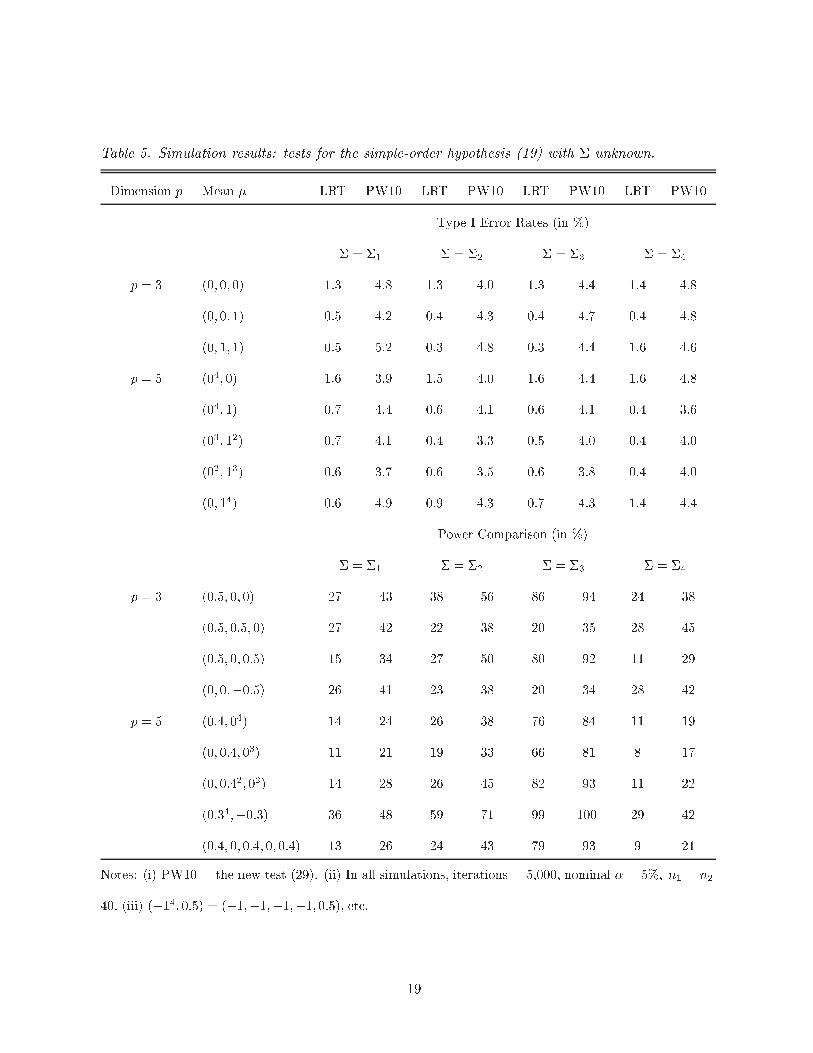
Table 5. Simulation results: tests for the simple-order hypothesis (19) with � unknown.

Dimension p Mean � LRT PW10 LRT PW10 LRT PW10 LRT PW10

Type I Error Rates (in %)

� = �1 � = �2 � = �3 � = �4

p = 3 (0; 0; 0) 1.3 4.8 1.3 4.0 1.3 4.4 1.4 4.8

(0; 0; 1) 0.5 4.2 0.4 4.3 0.4 4.7 0.4 4.8

(0; 1; 1) 0.5 5.2 0.3 4.8 0.3 4.4 1.6 4.6

p = 5 (04; 0) 1.6 3.9 1.5 4.0 1.6 4.4 1.6 4.8

(04; 1) 0.7 4.4 0.6 4.1 0.6 4.1 0.4 3.6

(03; 12) 0.7 4.1 0.4 3.3 0.5 4.0 0.4 4.0

(02; 13) 0.6 3.7 0.6 3.5 0.6 3.8 0.4 4.0

(0; 14) 0.6 4.9 0.9 4.3 0.7 4.3 1.4 4.4

Power Comparison (in %)

� = �1 � = �2 � = �3 � = �4

p = 3 (0:5; 0; 0) 27 43 38 56 86 94 24 38

(0:5; 0:5; 0) 27 42 22 38 20 35 28 45

(0:5; 0; 0:5) 15 34 27 50 80 92 11 29

(0; 0;�0:5) 26 41 23 38 20 34 28 42

p = 5 (0:4; 04) 14 24 26 38 76 84 11 19

(0; 0:4; 03) 11 21 19 33 66 81 8 17

(0; 0:42; 02) 14 28 26 45 82 93 11 22

(0:34;�0:3) 36 48 59 71 99 100 29 42

(0:4; 0; 0:4; 0; 0:4) 13 26 24 43 79 93 9 21

Notes: (i) PW10 = the new test (29). (ii) In all simulations, iterations = 5,000, nominal � = 5%; n1 = n2 =

40: (iii) (�14; 0:5) = (�1;�1;�1;�1; 0:5), etc.

19

better adaption to the dimensionalities of the boundary faces of �H0, thus better representing the

evidence provided by the data, as discussed in Section 2, rather than directly on consideration of

sizes and powers.

5 Examples

5.1 Example 1

Here we consider a model selection example for �nding true phylogenies. The data set, previously

analyzed in Shimodaira and Hasegawa (1999) and Shimodaira (2000), contains mitochondrial protein

sequences of 3414 amino acides for six mammal species (human, harbor seal, cow, rabbit, mouse,

and opossum). There are 105 possible phylogenies for the six species. We are interested in �nding

the true phylogeny | the hypothetical tree of the evolution history. As discussed in Shimodaira and

Hasegawa (1999), each phylogeny can be represented as a probabilistic model Mi, i = 0; 1; : : : ; 105,

and the maximized log-likelihood of Mi, denoted by Yi, is approximately normal. As illustration,

here we consider p = 5 phylogenies selected from 15 most probable phylogenies (see Shimodaira,

2000). Let E(Yi) = �i and �jk = �j � �k = E(Yj � Yk); j; k = 0; 1; : : : ; p. As in Shimodaira (2000),

we consider a (1��)�100% con�dence set for the true phylogenies. This can be achieved by testing

each H(k)0 : maxj 6=k �jk � 0 versus H

(k)1 : not H

(k)0 , k = 0; 1; : : : ; p, and determining the indices k

for which H(k)0 is not rejected at level �. Thus each test corresponds to testing problem (1) � (2)

with � unknown (see Section 3.3).

We index the p = 5 phylogenies based on the order of �Yk = maxj 6=k(Yj�Yk); k = 0; 1; 2; 3; 4

(from smallest to largest), and obtain (�Y0;�Y1;�Y2;�Y3;�Y4) = (0:0; 19:5; 22:7; 29:1; 33:6). At

the 90% con�dence level, the three tests in Section 3.3, LRT, UIT, and the new test PW4, produce

the same con�dence set which covers all 5 phylogenies. However, at 80% con�dence level, the

20

con�dence set based on LRT is f1; 2; 3; 4; 5g, the con�dence set based on UIT is f1; 2; 3g, and the

con�dence set based on PW4 is f1; 2; 3; 4g. Therefore, the three tests may produce di�erent results.

Based on the simulations in Section 3.3, the new test PW4 should provide the most reliable results.

5.2 Example 2

We consider a longitudinal study on the change of mental distress of parents whose children died by

accident. Data were collected on parents at 3 month, 6 month, and 18 month after their children's

death (Murphy et al. 2003). Mental distress was measured in terms of depression, anxiety, hostility,

somatization, and so on at each time point. We focus on the depression data, and only consider

male parents in the treatment group whose children were over 20 year-old and died by accident.

A total of n = 11 parents have depression data available at all three time points. Let Y1; Y2; and

Y3 denote depression measurements at month 3, 6, and 18 post-death. Let �i = E(Yi); i = 1; 2; 3:

We are interested in testing whether depression decreases over time, that is, we would like to test

H0 : �3 � �2 � �1 versus H1 : not H0, which corresponds to testing problem (19) in Section 4.2.

It appears that a multivariate normality assumption may be reasonable based on exploratory

analyses. The sample mean, sample covariance, and correlation matrices are

( �Y1; �Y2; �Y3) = (0:60; 0:97; 0:73); �̂ =

0BBBBBBB@0:32 0:63 0:40

0:63 1:51 0:92

0:40 0:92 0:57

1CCCCCCCA; R̂ =

0BBBBBBB@1 0:91 0:94

0:91 1 0:99

0:94 0:99 1

1CCCCCCCA;

respectively. At the 5% level, the LRT in Section 4.2 fails to reject H0, while the new test PW10

rejects H0, suggesting that the depression of fathers does not decrease over time. Based on the

simulation studies, the results from the new test PW10 should be more reliable. Thus, we conclude

that depression of the fathers does not decrease over time. A more thorough analysis will be reported

separately.

21

6 Discussion

The normality assumption in the article may be relaxed. When normality is not satis�ed, we may

use bootstrap methods, as in Shimodaira (2000) and Bloch et al. (2001). In such cases, we may let

the test statistics remain the same, but use bootstrap methods to obtain the critical values. The

implementation may be straightforward but it can be computationally intensive.

The testing problems we have considered are common in applications such as selection and

ranking problems and clinical trials with multiple endpoints. The LRT/UIT are still widely used

in these situations, but our results indicate that our proposed new tests do provide substantial

improvement for testing multivariate one-side hypotheses.

Acknowledgement. The authors thank Professor Ajit Tamhane for helpful comments and sug-

gestions.

References

Bloch, D.A., Lai, T.L., and Tubert-Bitter, P. (2001). One-sided tests in clinical trials with multiple

endpoints. Biometrics 57, 1039-1047.

Hsu, J.C. (1996). Multiple Comparisions { Theory and Methds. Chapman and Hall, London/New

York.

Murphy, S.A., Johnson, L.C., Wu, L., Fan, J.J., Lohan, J. (2003). \Bereaved Parents' Outcomes 4

to 60 Months After Their Children's Deaths by Accident, Suicide, or Homicide: A Comparative

Study Demonstrating Di�erences." Death Studies, 27, 39-61.

O'Brien, P.C. (1984). Procedures for comparing samples with multiple endpoints. Biometrics 40,

1079-1087.

22

Perlman, M.D. (1969). One-sided testing problems in multivariate analysis. Annals of Statistics

40, 549-567.

Perlman, M. D. and Wu, L. (1999). The Emperor's new tests (with discussion). Statistical Science

14 355-381.

Perlman, M. D. and Wu, L. (2002). On the Validity of the Likelihood Ratio and Maximum Likeli-

hood Methods. Journal of Statistical Planning and Inference 117, 59-81.

Perlman, M. D. and Wu, L. (2004). A Note on One-Sided Tests with Multiple Endpoints. Biomet-

rics, to appear.

Robertson, T., Wright, F. T., and Dykstra, R. L. (1988), Order-Restricted Statistical Inference. New

York: Wiley.

Shimodaira, H. (2000). Approximately unbiased one-sided tests of the maximum of normal means

using iterated bootstrap corrections. Tech. Report No. 2000-07, Dept. of Statistics, Stanford

University, Stanford, CA.

Shimodaira and Hasegawa (1999). Multiple comparisons of log-likelihoods with applications to

phylogenetic inference. Mol. Biol. Evol. 16, 1114-1116.

Tamhane, A.C. and Logan, B.R. (2004). A superiority-equivalence approach to one-sided tests on

multiple endpoints in clinical trials. To appear in Biometrika.

Tang, D.-I. (1994). Uniformly more powerful tests in a one-sided multivariate problem. Journal of

the American Statistical Association 89, 1006 - 1011.

Wollan, P.C. and Dykstra, R.L. (1987). Algorithm AS 225, Applied Statistics, 36, 234-240.

23

X1

X2

UITLRT

bX�

a2;�

u2;�

b PW1

~a2;�~a1;� = l1;�

~a1;�

PW3

l2;�

Figure 1. Rejection/acceptance regions of various tests for (1) � (2) with � known (� = I).

p = 2; � = 0:05; u2;� = 1:95; a2;� = 2:05; ~a1;� = 1:64; ~a2;� = 2:33. l1;� = 1:64; l2;� = 2:19:

24

y3

y1 y2

y1 = y2 < y3 y1 < y2 = y3

Figure 2. Rejection/acceptance regions of the LRT and the new test PW9 for (19) with � known

(� = I). LRT: dotted line, PW9: dashed line

25