SOME Lp-IMPROVING BOUNDS FOR RADON-LIKETRANSFORMS

Dominick Villano

A DISSERTATION

in

Mathematics

Presented to the Faculties of the University of Pennsylvania in PartialFulfillment of the Requirements for the Degree of Doctor of Philosophy

2019

Supervisor of Dissertation

Philip Gressman, Professor of Mathematics

Graduate Group Chairperson

Julia Hartmann, Professor of Mathematics

Dissertation Committee:Philip Gressman, Professor of MathematicsRyan Hynd, Professor of MathematicsFlorian Pop, Samuel D. Schack Professor of Algebra

ProQuest Number:

All rights reserved

INFORMATION TO ALL USERSThe quality of this reproduction is dependent upon the quality of the copy submitted.

In the unlikely event that the author did not send a complete manuscriptand there are missing pages, these will be noted. Also, if material had to be removed,

a note will indicate the deletion.

ProQuest

Published by ProQuest LLC ( ). Copyright of the Dissertation is held by the Author.

All rights reserved.This work is protected against unauthorized copying under Title 17, United States Code

Microform Edition © ProQuest LLC.

ProQuest LLC.789 East Eisenhower Parkway

P.O. Box 1346Ann Arbor, MI 48106 - 1346

13862139

13862139

2019

Acknowledgments

Thanks to Phil Gressman for guidance and patience. Thanks to Ryan Hynd and

Florian Pop for agreeing to be on my committee. Extra big time thanks to my

friends and family.

ii

ABSTRACT

SOME Lp-IMPROVING BOUNDS FOR RADON-LIKE TRANSFORMS

Dominick Villano

Philip Gressman

We prove Lp − Lq boundedness for a wide class of Radon-like transforms. The

technique of proof leverages the existing one-dimensional theory to produce a non-

trivial bounds in any dimension. For certain combinatorially simple transforms,

this range is sharp up to endpoints. Additionally, we make observations connecting

the Lp-improving properties of a Radon-like transform to the zero set of certain

homogeneous polynomials.

iii

Contents

1 Introduction 1

1.1 Background . . . . . . . . . . . . . . . . . . . . . . . . . . . . . . . 1

1.2 Definitions and Main Results . . . . . . . . . . . . . . . . . . . . . 6

2 Direct Bases and Sufficiency 10

2.1 Existence of Direct Bases . . . . . . . . . . . . . . . . . . . . . . . . 10

2.2 Trading Multilinearity for Dimensions . . . . . . . . . . . . . . . . . 12

2.3 Proof of Theorem 1.2.4 . . . . . . . . . . . . . . . . . . . . . . . . . 15

2.4 Tensor Decomposition and Optimization . . . . . . . . . . . . . . . 20

3 Split bases and Necessity 25

4 Examples and Sharpness 35

4.1 Convolution with the k-flat corkscrew, a flat sharp example . . . . . 35

4.2 A sharp example which is not flat, combinatorial flatness . . . . . . 37

4.3 Translation Invariant averages . . . . . . . . . . . . . . . . . . . . . 39

iv

4.4 The case of Hypersurfaces, a result of Seeger . . . . . . . . . . . . . 41

v

Chapter 1

Introduction

1.1 Background

Interesting Lesbesgue space mapping properties of the classical Radon transform can

be traced back to the work of Oberlin and Stein in [OS82]. For a Borel-measurable

function f : Rd → R, an element of the unit sphere u ∈ Sd−1, and a real number t,

define the Radon transform of f as follows

Rdf (u, t) :=

∫x·u=t

f (x) dσ1 (x) .

Here dσ is the induced d− 1 dimensional Lebesgue measure on each hyperplane.

It is is a simple consequence of Fubini’s theorem that Rd is bounded from L1 (R)

to L1(Sd−1 × R

). What Oberlin and Stein observed is that Rd is in fact bounded

from L(d+1)/d(Rd)

to Ld+1(Sd−1 × R

). This can be interpreted as a statement that

locally integrability becomes less wild after averaging in a suitable manner.

1

In fact, the local mapping properties of geometric averaging operators predates

the work of Oberlin and Stein. Interest in the problem dates at least as far back as

the 1970’s to work of Littman [Lit73] and Strichartz [Str70]. They were interested

in convolutions with singular measures supported on a hypersurface, in particular

the sphere. Precisely, they show that if f is Borel measurable and dσ2 is the surface

measure on the d − 1 dimensional unit sphere, then the operator TS,d defined via

the formula

TS,df (x) :=

∫Sd−1

f (x− y) dσ (y)

is bounded from Lp(Rd)

to Lq(Rd)

if and only if(

1p, 1q

)lies in the closed triangle

with vertices (0, 0) , (1, 1) ,(

dd+1

, 1d+1

)As in the case of the classical Radon transform, curvature plays a key role in the

local Lp-improving properties of the operator. The notion of rotational curvature

introduced by Phong and Stein in [PS86a, PS86b, PS91] unifies the classical Radon

transform and the spherical averaging operator. They show that, for hypersurfaces,

the best possible mapping properties of a geometric averaging operator are related to

the nonvanishing of a Monge-Ampere determinant. Specifically, if Φ : Rd×Rd → R

and

det

0 ∇xΦ

(∇yΦ)T ∂2Φ∂xi∂yj

6= 0,

then the operator

TΦf (x) :=

∫Φ(x,y)=0

f (y) a (a) dσx (y)

2

is bounded from L2(Rd)

to L2(d−1)/2

(Rd). This gain in Sobolev regularity then al-

lows (for instance), the argument of Strichartz to be applied and recover exactly the

same Lp mapping region as the spherical averaging operator. Although rotational

curvature fills the role of a necessary and sufficient condition for the best possible Lp

improving properties of a geometric averaging operator, no such condition correctly

exists in less favorable conditions, even for hypersurfaces.

Eventually, a more general but less quantitative result was obtained in landmark

work of Chirst, Nagel, Stein, and Wainger [CNSW99]. They introduce vector field

techniques which demand a rephrasing of the problem in order to state. This is the

formulation that will be used for the remainder of the thesis.

Let U ⊂ Rd be a small neighborhood of the origin. Suppose π1 : U → Rd−k1 and

π2 : U → Rd−k2 are smooth submersions. The projections πi generate a Radon-like

transform R, which is defined via duality

∫Rd−k2

Rf (y) g (y) dy :=

∫U

f (π1 (x)) g (π2 (x)) a (x) dx. (1.1.1)

Here a is a smooth cutoff function supported in U . Note that this operator is now

entirely local, and so is bounded from Lp to Lq for 1 ≤ q ≤ p by Holder’s inequality.

Additionally, since the Lp spaces are nested on a compact set, any nontrivial bound

corresponds to a gain in integrability, earning the title Lp-improving.

What Chirst, Nagel, Stein, and Wainger demonstrated is that Lp-improving

estimates exist if and only if the distributions kerDπ1 and kerDπ2 generate the

entire tangent space under the Lie Bracket. In the case of hypersuface averages, we

3

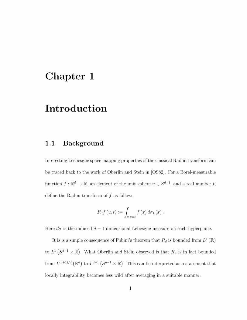
have the numerology k1 = k2 and d = 2k1 − 1. Additionally, kerDπ1 and kerDπ2

intersect trivially and rotational curvature translates as follows: for any smooth

nonzero vector field X defined on the support of a with X (x) ∈ kerDπ1 (x), there

is a smooth vector field Y ∈ kerDπ2 such that kerDπ1, kerDπ2 and [X, Y ] span

the tangent space.

As the higher dimensional theory was developing, a breakthrough for the case

of averaging over curves occurred in Christ’s 1998 paper “Convolution, Curvature,

and Combinatorics: a case study” [Chr98]. The paper obtains essentially optimal

restricted weak type bounds for the operator given by

Tγf (x) :=

∫ 1

−1

f(x−

(t, t2, . . . , td−1, td

))dt.

Chirst’s main innovation is to introduce a singular coordinate system by iterating

the above map. The singularities of this system are then carefully avoided using

what has now become know as the method of refinements.

The power of this philosophy can be seen in the work of Tao and Wright [TW03],

who synthesized the vector field techniques of Christ, Nagel, Stein, and Wainger

and iteration techniques of Christ to obtain optimal-up-to-endpoint restricted weak

type bounds of averages over any smooth family of curves. Of particular note is

their notion of a set of central width, which allows the method of refinements to

be executed even without explicit knowledge of the coordinate system’s singulari-

ties. This concept has no obvious higher-dimensional analogue. Another important

innovation is their theory of two-parameter Carnot-Caratheodory balls, which gen-

4

eralizes the one-parameter work of Nagel, Stein, and Wainger [NSW85].

Other signifigant and interesting results include the work of Bak [Bak00], Choi

[Cho11, Cho03], Christ, Dendrinos, Stovall, and Street [CDSS17], Dendrinos, Laghi,

and Wright [DLW09], Drury and Guo [DG91], Erdogan and Oberlin [EO10], Gress-

man [Gre09, Gre15], Lee [Lee04], Secco [Sec99]. Sharp bounds were obtained by

Iosevich and Sawyer [IS96] in the case that the geometry is given by homogeneous

polynomials. This thesis provides an alternate proof Seeger’s Lp-mapping theorem

in [See98]. Finally, in [Gre16], Gressman provides a curvature conditions which

fills the role of rotational curvature in certain situations: they ensure the largest

possible range of boundedness up to endpoints.

Of particular signifigance to the present thesis is the work of Street [Str11, Str14]

and Stovall [Sto11]. In [Str11, Str14], Streeet generalizes and refines the theory of

two paramater balls to multiparameter balls. In [Sto11], Stovall generalizes the

results of [TW03] to the multilinear setting.

The rotational curvature assumption of Phong and Stein, the one-dimensional

work of Tao and Wright, and the generalized curvature conditions of Gressman in

[Gre16] share two common features. First, up to endpoints, they produce the sharp

range of Lp−Lq boundedness. Second, they are all invariant under choice of vector

field, meaning that relevant spanning sets remain spanning after picking a different

basis of vector fields. This need not be the case in general.

The purpose of this thesis is to prove some bounds when such invariance is

5

not present. The strategy is to try to understand higher dimensional smooth dis-

tributions as the ensemble of all the smooth curves they contain. This is fairly

unwieldy and so some particularly useful families of vector fields are identified and

used to prove necessary and sufficient conditions. Sometimes these conditions align,

producing bounds that are sharp up to endpoints.

1.2 Definitions and Main Results

We will deal exclusively with Banach space exponents; all pi mentioned will satisfy

1 ≤ pi ≤ ∞.

We will introduce all Radon-like transforms via the double fibration formulation

(1.1.1). So, let d ≥ 4 and let U ⊂ Rd be a small neighborhood of the origin.

Suppose π1 : U → Rd−k1 and π2 : U → Rd−k2 are smooth submersions and that

ker (Dπ1)∩ker (Dπ2) is trivial. Without loss of generality πi (0) = 0. For notational

ease, let k3 = d− k1 − k2 and define

∆i := ker (Dπi) .

The projections πi generate a Radon-like transform R, which is defined via duality

∫Rd−k2

Rf (y) g (y) dy :=

∫U

f (π1 (x)) g (π2 (x)) a (x) dx.

Here a is a smooth cutoff function supported in U .

If there is a positive constant C such that for all measurable functions f1, f2, and

6

all smooth cutoff functions a with sufficiently small support, we have the inequality∫U

f (π1 (x)) g (π2 (x)) a (x) dx ≤ C ‖f‖Lp1(Rd−k1) ‖g‖Lp2(Rd−k2) , (1.2.1)

we say R is of strong type (p1, p′2), where 1/p+ 1/p′ = 1.

If there is a positive constant C ′ such that for all measurable subset E ⊂ Rd−k1 ,

F ⊂ Rd−k2 , and all smooth cutoff functions a with sufficiently small support, we

have the inequality∫U

χE (π1 (x))χF (π2 (x)) a (x) dx ≤ C ′ |E|1/p1 |F |1/p2 , (1.2.2)

then we say R is of restricted weak type (p1, p′2). By real interpolation, a proof of

which may also be found [Gra14], if an operator T is restricted weak type p1,1, p2,1

and p1,2, p2,2, then T is strong-type p1,θ, p2,θ where 0 < θ < 1 and

p−1i,θ := θp−1

i,1 + (1− θ) p−1i,2 .

The constant implicit in the symbol . can depend only on the pi and πi.

In order to state the main results of this thesis, a special class of vector fields

associate to ∆1 and ∆2 must be identified.

Definition 1.2.1. A basis of (∆1,∆2) is a (labeled) collection

B := X1, . . . , Xk1+k2 of smooth vector fields defined on U that is point-wise

linearly independent and satisfies Xi ∈ ∆1 for i ≤ k1, Xi ∈ ∆2 for i > k1.

We will be interested in spanning conditions of certain subsets of bases, and

so need to introduce a bookkeeping system. The following definitions are slight

variations of terminology appearing in [TW03] and [Sto11].

7

Definition 1.2.2. If B is a basis of (∆1,∆2) and S ⊆ B, let ∆S be the distribution

spanned by the Lie algebra generated by S. If dim ∆S/ (∆1 ⊕∆2) = k3, S is called

spanning.

A word associated to S is a j-tuple w ∈ 1, . . . , |S|j for some j ≥ 1. The

degree of a word is the ordered pair degw := (degw1, degw2) where degwi counts

the number of entries of w that belong to ∆i. If I is any finite collection of words,

deg I :=∑w∈I

degw.

Finally, to each word we assign a vector field, denoted Xw, defined via the recursive

formula:

X(w,j) := [Xw, Xj] .

Let W (S) denote the set of all words associated to S.

Bases that come equipped with a third, complementary distribution will be

important to the theory.

Definition 1.2.3. A basis B of (∆1,∆2) is called direct if [Xi, Xj] = 0 whenever

1 ≤ i, j ≤ k1 or k1 +1 ≤ i, j ≤ k1 +k2 and there exists a k3-dimensional distribution

∆3 with the following properties

1. Both ∆1 ∩∆3 and ∆2 ∩∆3 are trivial.

2. If w ∈ W (B) has length ≥ 2, Xw ∈ ∆3.

If S ⊆ B for some direct basis B, and S is spanning, write S ≺ (∆1,∆2). For such

S, if I is a finite collection of elements of W (S), I spans S if Xw (0) | w ∈ I spans

8

∆S (0). The mapping polytope of S, P (S) ⊂ R+ ×R+ is the interior of the convex

hull of the set

x | There exists some I that spans S with deg I ≤ x .

Here the inequality is taken coordinate-wise. Finally, the theorem:

Theorem 1.2.4. Suppose p1 ≥ 1, p2 ≥ 1, and p−11 + p−1

2 > 1. Define

(c1, c2) :=

(p2

p1 + p2 − p1p2

,p1

p1 + p2 − p1p2

).

Let P (∆1,∆2) be the interior of the convex hull of the union

⋃S≺(∆1,∆2)

P (S).

If

(c1, c2) ∈ P (∆1,∆2) ,

then R is of strong type (p1, p′2). In certain cases, this region is sharp up to end-

points, meaning that if the distance between P (∆1,∆2) and (b1, b2) is positive, then

R is not of strong type (p1, p′2).

The proof will proceed by proving the restricted weak type bound on the interior

of P (∆1,∆2). By real interpolation, the strong-type bound follows. There is a

corresponding necessary condition, which is used to prove sharpness, when possible.

This necessary condition involves a class of bases more general than direct bases.

Roughly speaking, theses will be bases for which minimal spanning sets correspond

to submanifolds. We delay the precise statements and proof.

9

Chapter 2

Direct Bases and Sufficiency

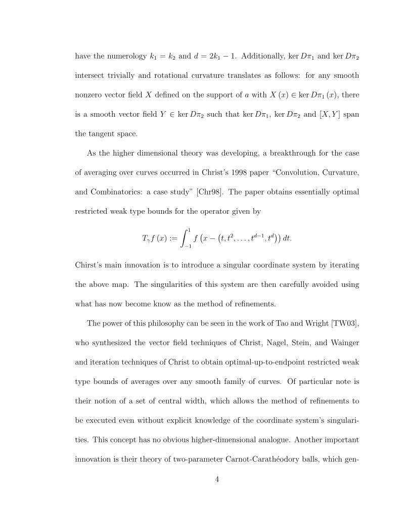
2.1 Existence of Direct Bases

It is not immediately clear from the definition that direct bases always exist. How-

ever, they do.

Lemma 2.1.1. Direct bases exist.

Proof. In a suitably small neighborhood of the origin, let Y1, . . . , Yd be pairwise

commuting, linearly independent vector fields such that Y1, . . . , Yk1 span ∆1. Let

Z1, . . . , Zk2 be an arbitrary basis of ∆2. Write Zi = Σai,jYj, where ai,j are smooth

functions. Since ∆1 and ∆2 span a k1 +k2 dimensional subspace at the origin, after

relabeling the Y ′j s if necessary, we may assume that the k2 rightmost columns of

the following matrix span a k2 dimensional subspace

10

A =

a1,1 a1,2 . . . a1,k1+k3 a1,k1+k3+1 . . . a1,d

a2,1 a2,2 . . . a2,k1+k3 a2,k1+k3+1 . . . a2,d

......

. . ....

.... . .

...

ak2,1 ad,2 . . . ak2,k1+k3 ak2,k1+k3+1 . . . ak2,d

.

Restricting to a possibly smaller neighborhood to avoid the zero set of certain

functions and again relabeling the Yj’s if necessary, A may be row reduced to obtain

A =

a1,1 a1,2 . . . a1,k1+k3 1 0 . . . 0

a2,1 a2,2 . . . a2,k1+k3 0 1 . . . 0

......

. . ....

......

. . ....

ak2,1 ad,2 . . . ak2,k1+k3 0 0 . . . 1

.

Define

Zi := Σai,jYj + Yk1+k3+i.

Since each Zi is a linear combination of Z1, . . . , Zk2 (with smooth functions for

coefficients),Z1, . . . , Zk2

spans ∆2. Further, any nonzero vector field in ∆2 must

have nonzero Yj coefficient for some j ≥ k1+k3+1. Since ∆2 is involutive [Zi, Z`] = 0

for all 1 ≤ i, ` ≤ k2.

Finally, there is a a smooth k1 + k3 dimensional distribution Σ1 that contains

∆1 (namely the span of Y1, . . . , Yk1+k3) and has trivial intersection with ∆2, such

that for any Y ∈ ∆1 and any 1 ≤ i ≤ k2, [Y, Zi] ∈ Σ1.

Repeating this argument with the roles of ∆1 and ∆2 reversed yields a k2 + k3

dimension distribution Σ2 containing ∆2 such that Σ2∩∆1 is trivial and a pairwise-

11

commuting collection of vector fields Y1, . . . , Yk1 that span ∆1 with the following

property: for any Z ∈ ∆2 and any 1 ≤ j ≤ k1, [Z, Yj, ] ∈ Σ2.

Set B :=Y1, . . . , Yk1 , Z1, . . . , Zk2

. Then any w ∈ W (B) of length ≥ 2 lies

in Σ1 ∩ Σ2, which is k3 dimensional and has trivial intersection with both ∆1 and

∆2.

2.2 Trading Multilinearity for Dimensions

Before moving on to a proof of the Theorem 1.2.4, we first record a brief but

useful method for translating multilinear, one-dimensional estimates to the higher

dimensional bilinear setting. We prove a quantitative version the of Hormander

implies Lp-improving result of Christ, Nagel, Stein, and Wainger [CNSW99] as a

consequence.

Suppose V ⊂ Rd is a suitably small neighborhood of the origin and that π1 :

V → Rd1 , π2 : V → Rd2 are smooth submersions with kerDπ1 ⊂ kerDπ2. Then for

any measurable subset Ω ⊂ V ,

|π1 (Ω)| . |π2 (Ω)| (2.2.1)

Here the implicit constant depends on V .

Proof. Since π1 is a submersion, π1 (Ω) is open and bounded. There is a third

smooth submersion π3 : π1 (Ω)→ Rd2 such that π3 π1 = π2. So

|π1 (Ω)| =∫π2(Ω)

f (x) dx

12

where f (x) ≤ supx∣∣π−1

3 (x)∣∣ . 1

This simple fact links one-dimensional, multilinear estimates to bilinear, high

dimensional estimates, which we state in the geometric, restricted weak-type for-

mulation.

Lemma 2.2.1. Suppose X1, . . . , Xk1+k2 are smooth, non-vanishing vector fields

on U satisfying Xi (x) ∈ ∆1 (x) for i ≤ k1 and Xi (x) ∈ ∆2 (x) for i > k1. Let πXi

be smooth submersions on U such that Xi spans kerDπXi. If (b1, . . . , bk1+k2) are

non-negative real numbers such that for all measurable subsets Ω ⊂ U

k1+k2∏i=1

(|Ω|

|πXi(Ω)|

)bi 1

|Ω|. 1 (2.2.2)

then (|Ω||π1 (Ω)|

)B1(|Ω||π2 (Ω)|

)B2 1

|Ω|. 1

where B1 :=∑k1

i=1 bi and B2 :=∑k1+k2

i=k1+1 bi.

Proof. Using (2.2.1), the proof is a simple calculation:(|Ω||π1 (Ω)|

)B1(|Ω||π2 (Ω)|

)B2 1

|Ω|

=

k1∏i=1

(|πXi

(Ω)||π1 (Ω)|

)bi k1+k2∏i=k1+1

(|πXi

(Ω)||π2 (Ω)|

)bi k1+k2∏i=1

(|Ω|

|πXi(Ω)|

)bi 1

|Ω|. 1

In [Sto11], Stovall classifies (up to endpoints), the tuples (b1, . . . , bk1+k2) for

which (2.2.2) holds. We recall one piece of terminology from that paper, as it will

be used more than once.

13

Definition 2.2.2. If S := X1, . . . , Xk1+k2 is a collection of smooth non-vanishing

vector fields on U , not necessarily linearly independent, such that Xi ∈ ∆1 for

i ≤ k1 and Xi ∈ ∆2 for i > k1, write S 5 (∆1,∆2). For w ∈ W (S), the multilinear

degree of w is the k1 + k2-tuple

degMLw := (degMLw1, . . . , degMLwk1+k2)

where degMLwi counts the number of occurrences of Xi in w. If I ∈ (W (S))d,

degML I =∑w∈I

degw.

We say I is spanning if Xw (0) | w ∈ I is linearly independent. Then, the multi-

linear polytope of S, PML (S) ⊂ Rk1+k2 , is the the interior of the convex hull of the

region

x | x ≥ degML I for some spanning I .

Corollary 2.2.3 (Quantitative Homander implies Lp-improving). Suppose that

(c1, c2) ∈⋃

S5(∆1,∆2)

⋃(b1,...,bn)∈PML(S)

(k1∑i=1

bi,

k2∑i=1

bi

).

Then R is of strong type (p1, p′2).

Proof. Fix some S such that (c1, c2) lies in the above region. Let πXibe as in

Lemma 2.2.1. Then (2.2.2) is satisfied by work of Stovall [Sto11], and the corollary

follows by Lemma 2.2.1.

In principle, it could be that Theorem 1.2.4 provides no new bounds beyond

those provided by Corollary 2.2.3, which, evidently, has a very brief proof. However,

14

we know of no such example at the moment. See the section concerning symmetry

and tensor decomposition for a more through discussion.

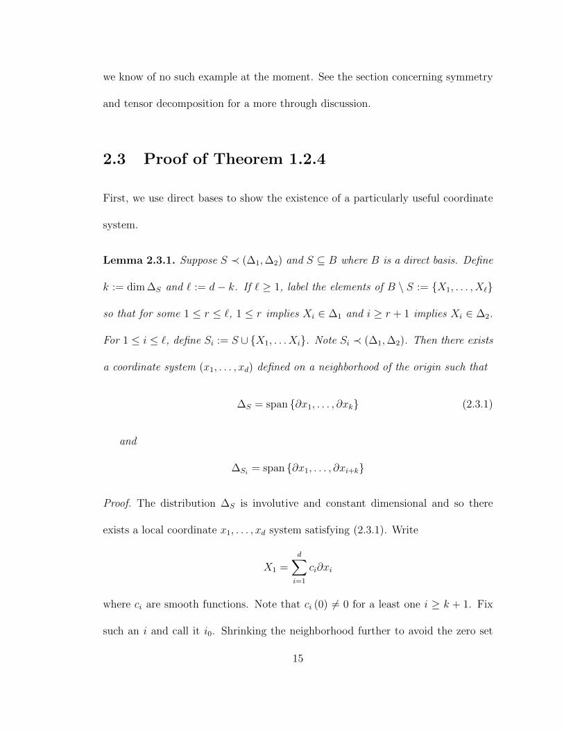
2.3 Proof of Theorem 1.2.4

First, we use direct bases to show the existence of a particularly useful coordinate

system.

Lemma 2.3.1. Suppose S ≺ (∆1,∆2) and S ⊆ B where B is a direct basis. Define

k := dim ∆S and ` := d− k. If ` ≥ 1, label the elements of B \ S := X1, . . . , X`

so that for some 1 ≤ r ≤ `, 1 ≤ r implies Xi ∈ ∆1 and i ≥ r + 1 implies Xi ∈ ∆2.

For 1 ≤ i ≤ `, define Si := S ∪ X1, . . . Xi. Note Si ≺ (∆1,∆2). Then there exists

a coordinate system (x1, . . . , xd) defined on a neighborhood of the origin such that

∆S = span ∂x1, . . . , ∂xk (2.3.1)

and

∆Si= span ∂x1, . . . , ∂xi+k

Proof. The distribution ∆S is involutive and constant dimensional and so there

exists a local coordinate x1, . . . , xd system satisfying (2.3.1). Write

X1 =d∑i=1

ci∂xi

where ci are smooth functions. Note that ci (0) 6= 0 for a least one i ≥ k + 1. Fix

such an i and call it i0. Shrinking the neighborhood further to avoid the zero set

15

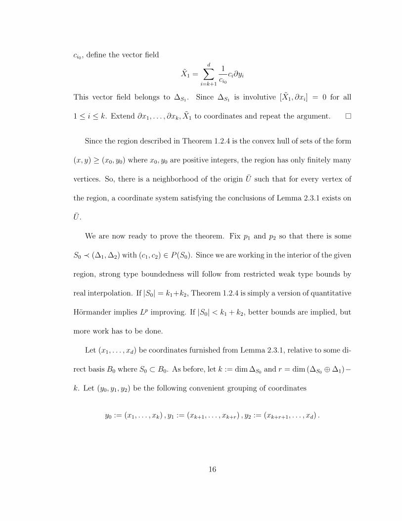
ci0 , define the vector field

X1 =d∑

i=k+1

1

ci0ci∂yi

This vector field belongs to ∆S1 . Since ∆S1 is involutive [X1, ∂xi] = 0 for all

1 ≤ i ≤ k. Extend ∂x1, . . . , ∂xk, X1 to coordinates and repeat the argument.

Since the region described in Theorem 1.2.4 is the convex hull of sets of the form

(x, y) ≥ (x0, y0) where x0, y0 are positive integers, the region has only finitely many

vertices. So, there is a neighborhood of the origin U such that for every vertex of

the region, a coordinate system satisfying the conclusions of Lemma 2.3.1 exists on

U .

We are now ready to prove the theorem. Fix p1 and p2 so that there is some

S0 ≺ (∆1,∆2) with (c1, c2) ∈ P (S0). Since we are working in the interior of the given

region, strong type boundedness will follow from restricted weak type bounds by

real interpolation. If |S0| = k1+k2, Theorem 1.2.4 is simply a version of quantitative

Hormander implies Lp improving. If |S0| < k1 + k2, better bounds are implied, but

more work has to be done.

Let (x1, . . . , xd) be coordinates furnished from Lemma 2.3.1, relative to some di-

rect basis B0 where S0 ⊂ B0. As before, let k := dim ∆S0 and r = dim (∆S0 ⊕∆1)−

k. Let (y0, y1, y2) be the following convenient grouping of coordinates

y0 := (x1, . . . , xk) , y1 := (xk+1, . . . , xk+r) , y2 := (xk+r+1, . . . , xd) .

16

For any measurable subset Ω, define the following slices:

Ω(y1,y2) := Ω ∩ (y0, y1, y2) | (y1, y2) = (y1, y2)

Ωy2 := Ω ∩ (y0, y1, y2) | y2 = y2 .

In particular, we have

U(y1,y2) := U ∩ (y0, y1, y2) | (y1, y2) = (y1, y2)

Uy2 := U ∩ (y0, y1, y2) | y2 = y2 .

Define si := dim ∆S0 − |S0 ∩∆i|. Note that s1 + d − (k + r) = d − k1 and

s2 + r = d − k2. For the next few calculations, we will include some normally

suppressed notation: if ρ is a positive integer and E is measurable |E|ρ indicates

the ρ-dimensional (induced) measures of E. By Corollary 2.2.3 applied to each of

the leaves of the foliation defined by ∆S

|Ω| =∫∫ ∣∣Ω(y1,y2)

∣∣kdy1dy2

.(y1,y2)

∫∫ ∣∣π1

(Ω(y1,y2)

)∣∣1/p1s1

∣∣π2

(Ω(y1,y2)

)∣∣1/p2s2

dy1dy2.

(2.3.2)

Then to prove the restricted weak-type analogue of (1.2.2), it suffices to show that

dependence of the constant on (y1, y2) can be removed and that

∫∫ ∣∣π1

(Ω(y1,y2)

)∣∣1/p1s1

∣∣π2

(Ω(y1,y2)

)∣∣1/p2s2

dy1dy2 . |π1 (Ω)|1/p1d−k1 |π2 (Ω)|1/p2d−k2 . (2.3.3)

We delay the proof of the former and focus just on (2.3.3). In general, bounding

the size of its projection by the size of some arbitrary slice is not possible. But in

17

this case, the interaction between the coordinates and the projections makes such

a bound possible and trivial: For each (y1, y2), there is a map

π(y1,y2)1 : Uy2 → U(y1,y2)

such that for all x ∈ Uy2 , π1 (x) = π1 π(y1,y2)1 (x) and for all measurable Ω ⊂ U ,

Ω(y1,y2) ⊂ π(y1,y2)1 (Ωy2) .

This means that

∣∣π1

(Ω(y1,y2)

)∣∣s1≤∣∣∣π1

(π

(y1,y2)1 (Ωy2)

)∣∣∣s1

= |π1 (Ωy2)|s1 . (2.3.4)

By a similar argument,

|πy22 (Ωy2)|d−k2 ≤ |π2 (Ω)|d−k2 (2.3.5)

The inequalities (2.3.4) and (2.3.5), along with Jensen’s inequality, transfer the

bound from a slice to the whole space:

∫∫ ∣∣π1

(Ω(y1,y2)

)∣∣1/p1s1

∣∣π2

(Ω(y1,y2)

)∣∣1/p2s2

dy1dy2

≤∫|π1 (Ωy2)|

1/p1s1

∫ ∣∣π2

(Ω(y1,y2)

)∣∣1/p2s2

dy1dy2

.∫|π1 (Ωy2)|

1/p1s1

(∫ ∣∣π2

(Ω(y1,y2)

)∣∣s2dy1

)1/p2

dy2

=

∫|π1 (Ωy2)|

1/p1s1|π2 (Ωy2)|

1/p2s2+r dy2

=

∫|π1 (Ωy2)|

1/p1s1|π2 (Ωy2)|

1/p2d−k2 dy2

≤∫|π1 (Ωy2)|

1/p1s1

dy2 |π2 (Ω)|1/p2d−k2 . |π1 (Ω)|1/p1d−k1 |π2 (Ω)|1/p2d−k2

18

Now we explain why the the implicit constant’s dependence on (y1, y2) can be re-

moved. This is because the implied constant in Stovall’s multilinear theory remains

bounded under small perturbation. Much of the work has already been done by

Street [Str11, Str14]. Specifically, Street shows that the implicit constants present

in all pertinent multi-parameter Carnot-Caretheodory ball estimates can be chosen

to depend only on the CM norms of the vector fields, provided that the parameter

ε can be bounded below. For more details, see Theorem 5.5 of [Str11].

This requirement on ε is not a problem, as the constant produced in the ex-

ponent when performing the refinement process in [Sto11] will behave well under

perturbation. This means that ε can be bounded from below, as the multilinear

polytope can only get bigger under a small perturbation.

The key inequalities in [Sto11] are

αbαCεk .∑I∈I0

δdegML I . B (x0; δ1, . . . , δk) ∼ Bj (x0; δ1, . . . , δk) (2.3.6)

and

αCεk Bj (x0; δ1, . . . , δk) .∣∣Φn

j (Tn)∣∣ . (2.3.7)

Here b is the relevant multilinear exponent, B and Bj are two types of multi-

paramater Carnot-Caretheodory balls, and Φnj (Tn) is a subset of Bj. See [Sto11]

for precise definitions. All implied constants depend on ε

By Street’s work [Str11], the implicit constant in the first two inequalities of

(2.3.6) can be taken uniform over a perturbation. The constant in last comparability

estimate of (2.3.6) can also be taken uniform, since the estimate follows from a com-

19

pactness argument whose main ingredient is a map associated to B (x0; δ1, . . . , δk),

whose implicit constant Street also controls.

There only remains the inequality in (2.3.7). This comes down to check the

hypotheses of Theorem 7.1 in Christ’s paper [Chr08]. Hypotheses (i) and (ii) are

certainly satisfied and Stovall’s method of checking of the third condition will also

remain valid after a small perturbation.

2.4 Tensor Decomposition and Optimization

It follows from the proof that, roughly, the smaller the S ≺ (∆1,∆2), the better

the bounds. More precisely, let S1, S2 ≺ (∆1,∆2) and suppose there are k3-tuples

of words of length at least two

(w1,1, . . . w1,k3) ∈ (W (S1))k3

(w2,1, . . . w2,k3) ∈ (W (S2))k3

such thatXw1,i

(0)

andXw2,j

(0)

are linearly independent and

∑i

degw1,i =∑j

degw2,j.

If |S1| < |S2|, then the techniques used in the proof of Theorem 1.2.4 produce a

strictly greater region of boundedness when using S1 and (w1,1, . . . w1,k3) than when

using S2 and (w2,1, . . . w2,k3).

Additionally, if Mi are non-singular ki× ki matrices and B := X1, . . . , Xk1+k2

20

is a direct basis of (∆1,∆2), then

B := M1 (X1) , . . . ,M1 (Xk1) ,M2 (Xk1+1) . . . ,M2 (Xk1+k2)

is also a direct basis of (∆1,∆2). Here we are identifying ∆i (0) with Rki and Xi

with elements of the appropriate standard basis. These two observations allow us to

shift the question of R’s boundedness to a question about the symmetry properties

of high-rank tensors.

Let B be a direct basis of (∆1,∆2) and let τ := (w1, . . . , wk3) a k3-tuple of words

of length at least two. If deg τ = (d1, d2), then τ produces a multilinear map

Tτ :(Rk1)d1 × (Rk2

)d2 → R.

The procedure is straightforward but notationally lengthy. First, let

XXX1 := (X1, . . . , Xk1) and XXX2 := (Xk1+1, . . . , Xk1+k2. For any u ∈ Rk1 and v ∈ Rk2

define

u ·XXX1 :=

k1∑i=1

uiXi, v ·XXX2 :=

k1+k2∑j=k1+1

vjXj

Then, for w` ∈ τ of degree (d1,`, d2,`), let Xw`

(u1, . . . , ud1,` , v1, . . . vd2,`

)be the vector

field obtained by taking the iterated commutator formula for Xw`and replacing the

ith occurrence of an element in XXX1 with ui ·XXX1 and the jth occurrence of an element

in XXX2 with vj ·XXX2. The map

Tw`

(u1, . . . , ud1,` , v1, . . . vd2,`

)= Xw`

(u1, . . . , ud1,` , v1, . . . vd2,`

)(0)

21

is a multilinear map from(Rk1)d1,` × (Rk2

)d2,` to ∆3 (0). Finally, define

Tτ

(u1

1, . . . , u1d1,1, v1

1, . . . v1d2,1, . . . , uk31 , . . . , u

k3d1,k3

, vk31 , . . . vk3d2,k3

):= detk3

(Tw1 , . . . , Twk3

)(0)

(2.4.1)

Here detk3 is the volume form on the leaf of ∆3 passing through the origin. The

symmetry properties of Tτ influence the analysis of R. However, the symmetry

properties of an arbitrarily high-rank tensor are hard to understand. Here we state

the general lemma, which may be useful in some applications, and a more spe-

cific lemma which can be used, for instance, in the case of translation invariant

convolution with a submanifold.

Lemma 2.4.1. Suppose that deg τ = (d1, d2), and for 1 ≤ r1 ≤ k1, 1 ≤ r2 ≤ k2

there is a r1dimensional subspace U ⊂ Rk1 and an r2- dimensional subspace V ⊂ Rk2

such that Tτ restricted to U × V is not identically zero. If

(c1, c2) ⊂x ∈ R2 | x > deg τ + (r1, r2)

,

then R is strong-type (p1, p′2).

Proof. Let e1, . . . , er1 be a basis of U and f1, . . . , fr2 a basis for V . There is a

d1-element sequence ei1 , . . . e1d1and d2-element sequence fj1 , . . . , fjd2 such that

Tτ

(ei1 , . . . e1d1

, fj1 , . . . , fjd2

)6= 0

This corresponds to an S ′ ≺ (∆1,∆2) with |S ′| = r1 + r2 and a τ ′ spanning S ′ with

deg τ ′ = τ + r1 + r2. The lemma follows by Theorem 1.2.4.

22

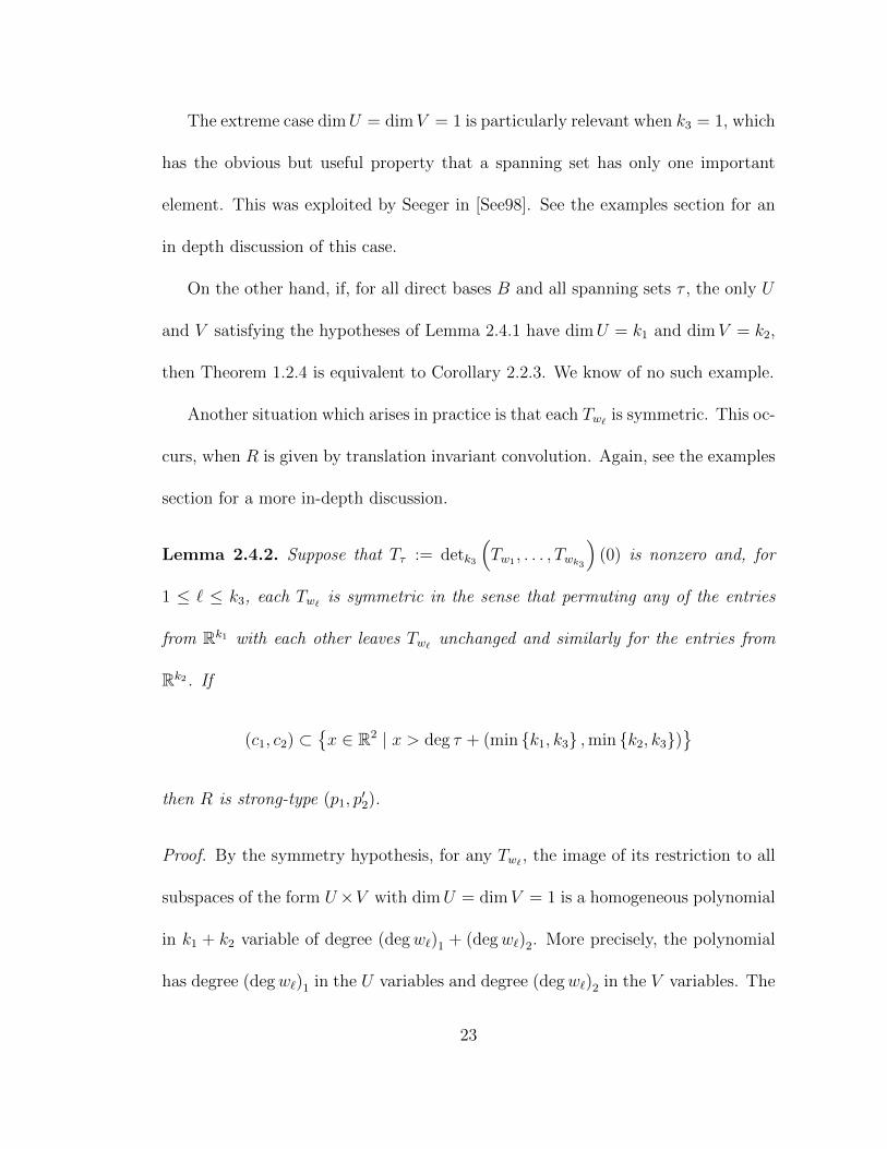
The extreme case dimU = dimV = 1 is particularly relevant when k3 = 1, which

has the obvious but useful property that a spanning set has only one important

element. This was exploited by Seeger in [See98]. See the examples section for an

in depth discussion of this case.

On the other hand, if, for all direct bases B and all spanning sets τ , the only U

and V satisfying the hypotheses of Lemma 2.4.1 have dimU = k1 and dimV = k2,

then Theorem 1.2.4 is equivalent to Corollary 2.2.3. We know of no such example.

Another situation which arises in practice is that each Tw`is symmetric. This oc-

curs, when R is given by translation invariant convolution. Again, see the examples

section for a more in-depth discussion.

Lemma 2.4.2. Suppose that Tτ := detk3

(Tw1 , . . . , Twk3

)(0) is nonzero and, for

1 ≤ ` ≤ k3, each Tw`is symmetric in the sense that permuting any of the entries

from Rk1 with each other leaves Tw`unchanged and similarly for the entries from

Rk2. If

(c1, c2) ⊂x ∈ R2 | x > deg τ + (min k1, k3 ,min k2, k3)

then R is strong-type (p1, p

′2).

Proof. By the symmetry hypothesis, for any Tw`, the image of its restriction to all

subspaces of the form U×V with dimU = dimV = 1 is a homogeneous polynomial

in k1 + k2 variable of degree (degw`)1 + (degw`)2. More precisely, the polynomial

has degree (degw`)1 in the U variables and degree (degw`)2 in the V variables. The

23

coefficients are various directions Xw (0), and if Tw`is not the zero map, at least

one of these is not zero.

Set all the V variables equal to one. Consider the (affine) Veronese map from

Rk1 → RN where N is the number of monomials of degree (degw`)1 in k1 variables:

x = (x1, . . . , xk1)→ (xα)|α|=(degw`)1.

Here the α are multiindices. The image of this map is not contained in any hyper-

plane, and so the restriction of Tw`is nonzero, as a polynomial.

To see that the restriction of Tτ is nonzero, notice that

detk3

(Tw1 , . . . , Twk3

)(0) 6= 0

implies the existence of words w′1, . . . , w′k3

such that Xw′1, . . . , Xw′k3

are linearly in-

dependent. Using the multi-linearity of the determinant expand the polynomial Tτ

yields a polynomial with at least one nonzero coefficient. Then the claim follows by

Lemma 2.4.1.

24

Chapter 3

Split bases and Necessity

We now give a necessary condition for R to be of strong type (p1, p′2). Like the

sufficient condition, it is phrased in terms of a special class of bases.

Definition 3.0.1. A basis B of (∆1,∆2) is called split if [Xi, Xj] = 0 when either

1 ≤ i, j ≤ k1 or k1 + 1 ≤ i, j ≤ k1 + k2 and for every vertex v of PML (B) there

exists some spanning I = w1, . . . , wd ∈ (W (B))d with the following properties.

(Here we make the labeling choice that that wi = i for 1 ≤ i ≤ k1 + k2.)

1. degML I = v

2. The distribution defined by

span Xwi| 1 ≤ i ≤ k1, 1 + k1 + k2 ≤ i ≤ d

is involutive on U .

25

3. The distribution defined by

span Xwi| 1 + k1 ≤ i ≤ d

is involutive on U .

Any I ∈ W (B)d satisfying these properties for some vertex v will be called split. If

B is split, write B (∆1,∆2).

Any direct basis is split, so Lemma 2.1.1 implies the existence of split bases as

well. There are split bases that are not direct. See the next section for a simple

example.

Split bases are bases for which minimal spanning sets correspond to submani-

folds.

Theorem 3.0.2. Let φ(k1,k2) : R2 → Rk1+k2 be the linear map defined by

φ(k1,k2) (x1, x2) = (x1, . . . , x1, x2, . . . , x2)

where x1 is repeated k1 times and x2 is repeated k2 times. Suppose p1 ≥ 1, p2 ≥ 1,

and p−11 + p−1

2 > 1. If

φ(k1,k2) (c1, c2) /∈⋂

B(∆1,∆2)

PML (B) ,

then R is not of restricted weak type (p1, p′2).

Proof. The strategy is to show that, if B is split basis of (∆1,∆2), and if φ (c1, c2) /∈

PML (B), then the counterexamples in the one-dimensional multilinear setting are

also counterexamples in the bilinear, high-dimensional situation.

26

If φ (c1, c2) does not lie in the region defined in the main theorem, there is a

split basis B0 such that φ (c1, c2) /∈ PML (B0). Let πXjbe a smooth submersion

which takes a U to Rd−1 with Xj tangent to its level sets. By work of Stovall, for

positive η small enough, there is a measurable set Ωη contained in some small

neighborhood of the origin such that as η → 0

Aη :=

k1∏j=1

(|Ωη|∣∣πXj

(Ωη)∣∣)c1 k1+k2∏

j=k1+1

(|Ωη|∣∣πXj

(Ωη)∣∣)c2

1

|Ωη|→ ∞.

Since

(|Ωη||π1 (Ωη)|

)c1 ( |Ωη||π2 (Ωη)|

)c2 1

|Ωη|=( ∏k1

j=1

∣∣πXj(Ωη)

∣∣|π1 (Ωη)| |Ωη|k1−1

)c1 (∏k1+k2j=k1+1

∣∣πXj(Ωη)

∣∣|π2 (Ωη)| |Ωη|k2−1

)c2

Aη,

to prove Theorem 3.0.2, it suffices to show∏k1j=1

∣∣πXj(Ωη)

∣∣|π1 (Ωη)| |Ωη|k1−1

∼ 1 (3.0.1)

and ∏k1+k2j=k1+1

∣∣πXj(Ωη)

∣∣|π2 (Ωη)| |Ωη|k2−1

∼ 1. (3.0.2)

Note that neither (3.0.1) and (3.0.2) involve any interaction between ∆1 and

∆2. The estimates are, in a sense, a statement about the rectangularity of Ωη in

two different coordinate systems.

To that end, here is a review of Stovall’s construction, which is influenced by the

work of Tao and Wright [TW03] and Chirst, Nagel, Stein, and Wainger [CNSW99].

27

Additionally, all of what follows can be placed in the more general work of Street

concerning multiparameter Carnot-Caretheodory balls.

In what follows, ε is a small positive parameter, and K is a large positive pa-

rameter. All implicit constants in this section depend on ε. If δ := (δ1, . . . , δk1+k2)

is some k1 + k2-tuple of small positive real numbers and I ∈ W (B0)d, define

(Kδ)degML I :=

k1+k2∏j=1

(Kδj)(degML I)j

Since (∆1,∆2) satisfy the Hormander condition, there is some

I ′ = w1, . . . , wd ∈ W (B0)d so that

λI0 (0) := det (Xw1 , . . . , Xwd) (0) 6= 0

Setting D :=∑k1+k2

j=1 (degML I′)j, define

I :=

I ∈ W (S0) : (degML I)j ≤

D

ε, 1 ≤ j ≤ k1 + k2

.

We will always assume ε is small enough that I contains all the vertices of PML (B0).

Since there are finitely many vertices of PML (B0), there are finitely many split

I ∈ W (B0)d, and by shrinking the neighborhood, we may assume that λI (x) ∼ 1

and

det(X1, . . . , Xk1 , Xwk1+k2+1

, . . . , Xwd

)(x) ∼ 1 (3.0.3)

det(Xk1+1, . . . , Xk1+k2 , Xwk1+k2+1

, . . . , Xwd

)(x) ∼ 1. (3.0.4)

for all split I. Here det is the induced volume form on the appropriate submanifolds,

which exist since I is split.

28

Then define the vector valued function

Λ (x) :=(

(Kδ)degML I λI (x))I∈I

There is some I0 ∈ I such that (Kδ)degML I0 λI0 (0) ∼ |Λ (0)|. In fact, if the entries

of δ are small enough, there is a split I0 satisfying the above. Fix this I0 :=

w1, . . . , wd and define the mapping

Φδ (t1, . . . , td) := exp

(d∑j=1

K−1 (Kδ)degML wj tjXwj

)(0) .

Since DΦ is nonsingular at the origin, the pullback vectors

Yw,δ := (DΦ)−1(K−1 (Kδ)degML wXw

)can be defined on a neighborhood on the origin, which, at first glance, may depend

on δ. In fact, the following lemma from [Sto11, TW03] guarantees that it does not.

It requires two more assumption on δ, which are usually called the smallness and

non-degeneracy conditions respectively

δj ≤ c (ε,K) , 1 ≤ j ≤ k1 + k2 (3.0.5)

δj ≤ Cδεi , 1 ≤ i, j ≤ k1 + k2 (3.0.6)

Here, c (ε,K) is a constand depending on ε and K, and C is a constant depending

on ε. Since the actual structure of Ωη matters, some facts about Φ from [Sto11] will

be important. The following lemma holds for all ε suitably small, K suitably large,

and δ satisfying the smallness and non-degeneracy conditions. In fact, this lemma

29

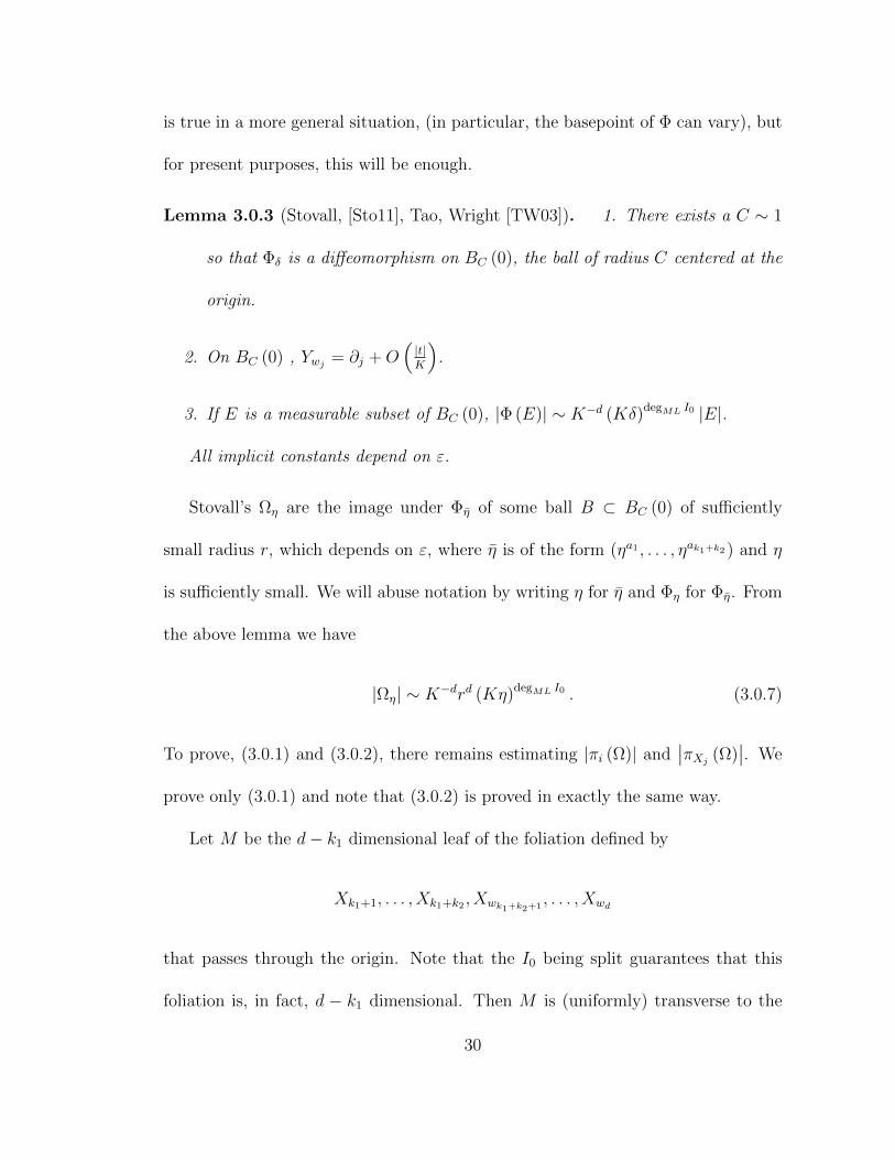
is true in a more general situation, (in particular, the basepoint of Φ can vary), but

for present purposes, this will be enough.

Lemma 3.0.3 (Stovall, [Sto11], Tao, Wright [TW03]). 1. There exists a C ∼ 1

so that Φδ is a diffeomorphism on BC (0), the ball of radius C centered at the

origin.

2. On BC (0) , Ywj= ∂j +O

(|t|K

).

3. If E is a measurable subset of BC (0), |Φ (E)| ∼ K−d (Kδ)degML I0 |E|.

All implicit constants depend on ε.

Stovall’s Ωη are the image under Φη of some ball B ⊂ BC (0) of sufficiently

small radius r, which depends on ε, where η is of the form (ηa1 , . . . , ηak1+k2 ) and η

is sufficiently small. We will abuse notation by writing η for η and Φη for Φη. From

the above lemma we have

|Ωη| ∼ K−drd (Kη)degML I0 . (3.0.7)

To prove, (3.0.1) and (3.0.2), there remains estimating |πi (Ω)| and∣∣πXj

(Ω)∣∣. We

prove only (3.0.1) and note that (3.0.2) is proved in exactly the same way.

Let M be the d− k1 dimensional leaf of the foliation defined by

Xk1+1, . . . , Xk1+k2 , Xwk1+k2+1, . . . , Xwd

that passes through the origin. Note that the I0 being split guarantees that this

foliation is, in fact, d − k1 dimensional. Then M is (uniformly) transverse to the

30

fibers of π1, and so π1 restricted to M is a diffeomorphism. Then, for any measurable

function f defined on a sufficiently small neighborhood U of Rd−k1 ,

∫U

f (y) dµ (y) ∼∫M

f π∆1 (x) dν (x) . (3.0.8)

Here dµ and dν are the densities that come from (restriction of) the volume form.

The ∼ comes from a determinant expression in the change of variables forumla,

which depends only on the geometry of the vector fields. The submanfold M is

well suited to Φη0 . Specifically, if V is the subspace of Rd with zeros in the first k1

components, then Φη (V ∩B) = M ∩ Ωη. By change of variables and (3.0.4)

∫M

f π1 (x)dν (x) =

∫V ∩BC

f π1 Φη (t)∣∣detDΦη (t)

∣∣ dt∼ K−(d−k1)

d∏j=k1+1

(Kη)degML wj

∫V ∩BC

f π1 Φη (t) dt.

(3.0.9)

Here Φη is the restriction of Φη to V . A few different choices of f will be useful.

For estimating |π1 (Ωη)|, define

f0 (y) :=

1 if π−1

1 (y) ∩ Ωη 6= ∅

0 else

Since Ywi= ∂i +O

(|t|K

), the set of t ∈ V such that f0 π1 Φη (t) 6= 0 contains

the set V ∩ Br and is contained in the set V ∩ B2r if K is sufficiently large. And

so, by (3.0.8) and (3.0.9)

|π1 (Ωη)| ∼ K−(d−k1)rd−k1d∏

i=k1+1

(Kη)degML wi . (3.0.10)

31

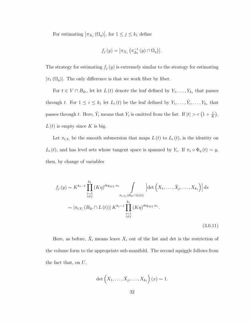
For estimating∣∣πXj

(Ωη)∣∣, for 1 ≤ j ≤ k1 define

fj (y) =∣∣πXj

(π−1

∆1(y) ∩ Ωη

)∣∣ .The strategy for estimating fj (y) is extremely similar to the strategy for estimating

|π1 (Ωη)|. The only difference is that we work fiber by fiber.

For t ∈ V ∩ B2r, let let L (t) denote the leaf defined by Y1, . . . , Yk1 that passes

through t. For 1 ≤ i ≤ k1 let Li (t) be the leaf defined by Y1, . . . , Yi, . . . , Yk1 that

passes through t. Here, Yi means that Yi is omitted from the list. If |t| > r(1 + 1

K

),

L (t) is empty since K is big.

Let πt,Yi be the smooth submersion that maps L (t) to Li (t), is the identity on

Li (t), and has level sets whose tangent space is spanned by Yi. If π1 Φη (t) = y,

then, by change of variables

fj (y) ∼ Kk1−1

k1∏i=1i 6=j

(Kη)degML wi

∫πt,Yi (B2r∩L(t))

∣∣∣det(X1, . . . , Xj, . . . , Xk1

)∣∣∣ ds∼ |πt,Yi (B2r ∩ L (t))|Kk1−1

k1∏i=1i 6=j

(Kη)degML wi .

(3.0.11)

Here, as before, Xi means leave Xi out of the list and det is the restriction of

the volume form to the appropriate sub-manifold. The second squiggle follows from

the fact that, on U ,

det(X1, . . . , Xj, . . . , Xk1

)(x) ∼ 1.

32

The last step is to understand |πt,Yi (B2r ∩ L (t))|, which is done by leaning on

the estimate Ywi= ∂i +O

(|t|K

). Let π be the map defined by

π (t1, . . . , td) := (t1, . . . , tk1) .

For t ∈ V ∩B, define

g (t) := max

0,

√r2 − |t|2

.

Let B′ be the d− k1 dimensional ball of radius r/K centered at the origin

h1 (t) := supb′∈B′

g (t− b′) , h2 (t) := infb′∈B

g (t− b′) .

If B (ρ) denotes the k1-dimensional ball centered at the origin of radius ρ, we have

B (h2 (t)) ⊂ π (L (t)) ⊂ B (h1 (t)) (3.0.12)

once again, because Ywi= ∂i +O

(|t|K

). The strategy is to show that

∫(h2 (t))k1 dt ∼

∫(h1 (t))k1 dt (3.0.13)

which means that π (L (t)) is more or less B (g (t)) This is essentially automatic, but

here is a double check that the estimate is independent of big K. Push everything

to polar coordinates and suppose, for instance, K > 10, then

∫(h1 (t))k1 dt ∼

( rK

)d−k1rk1 +

∫ r+r/K

r/K

td−k1−1

(r2 −

(t− r

K

)2)k1/2

dt

. rk1

(( rK

)d−k1+

∫ r+r/K

r/K

td−k1−1dt

). rd,

33

and

∫(h2 (t))k1 dt ∼

∫ r−r/K

0

td−k1−1

(r2 −

(t+

r

K

)2)k1/2

dt

&∫ r/2−r/K

0

td−k1−1

(r2 −

(t+

r

K

)2)k1/2

dt

& rk1∫ r/2−r/K

0

td−k1−1dt ∼ rd.

Then (3.0.12), (3.0.13) and the estimate Ywi= ∂i +O

(|t|K

)imply

∫V ∩B2r

|πt,Yi (B2r ∩ L (t))| dt ∼∫V ∩Br

(r2 − |t|2

) k1−12 dt ∼ rd−1.

Combined with (3.0.9) and (3.0.11), this gives

∣∣πXj(Ωη)

∣∣ ∼ K−(d−1)rd−1

d∏i=1i 6=j

(Kη)degML wi . (3.0.14)

With that (3.0.7), (3.0.10), and (3.0.14) established, (3.0.1) follows.

34

Chapter 4

Examples and Sharpness

4.1 Convolution with the k-flat corkscrew, a flat

sharp example

There are examples where the regions described in Theorem 1.2.4 and Theorem

3.0.2 coincide, meaning that, up to endpoints, the region is sharp. This is easiest

to see with examples that are flat in all but one direction. Specifically, if there is a

direct basis B := X1, . . . , Xk1+k2 such that i ≤ k1 − 1 or j ≤ k1 + k2 − 1 implies

[Xi, Xj] = 0,

then any word of length greater than two involved in a spanning set is a finite

sequence of only k1’s and k1 + k2’s. This immediately implies that the two regions

coincide, and that Theorem 1.2.4 is sharp up to endpoints. Here is an explicit

example:

35

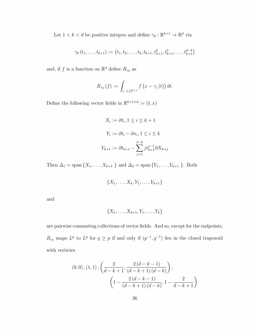
Let 1 < k < d be positive integers and define γ0 : Rk+1 → Rd via

γ0 (t1, . . . , tk+1) :=(t1, t2, . . . , tk, tk+1, t

2k+1, t

3k+1, . . . , t

d−kk+1

)and, if f is a function on Rd define Rγ0 as

Rγ0 (f) :=

∫[−1,1]k+1

f(x− γ) (t)

)dt.

Define the following vector fields in Rk+1+d := (t, x)

Xi := ∂ti, 1 ≤ i ≤ k + 1

Yi := ∂ti − ∂xi, 1 ≤ i ≤ k

Yk+1 := ∂tk+1 −d−k∑j=1

jtj−1k+1∂Xk+j

Then ∆1 = span X1, . . . , Xk+1 and ∆2 = span Y1, . . . , Yk+1 . Both

X1, . . . , Xk, Y1, . . . , Yk+1

and

X1, . . . , Xk+1, Y1, . . . , Yk

are pairwise commuting collections of vector fields. And so, except for the endpoints,

Rγ0 maps Lp to Lq for q ≥ p if and only if (p−1, q−1) lies in the closed trapezoid

with verticies

(0, 0) , (1, 1) ,

(2

d− k + 1,

2 (d− k − 1)

(d− k + 1) (d− k)

),(

1− 2 (d− k − 1)

(d− k + 1) (d− k), 1− 2

d− k + 1

)36

4.2 A sharp example which is not flat, combina-

torial flatness

Such totally flat examples are not the only case in which the region given in Theorem

1.2.4 is sharp. What is really important is the existence of a split basis in which

only one vector field from ∆1 and one vector field from ∆2 control the spanning

sets. Such pairs distributions might be called combinatorially flat.

In R4 consider the pair of distributions ∆1 := span ∂x1 , ∂x2 and

∆2 := span ∂x3 + (x1x3 + x2) ∂x4. Let RCF be the associated Radon-like trans-

form. The basis

B0 = ∂x1 , ∂x2 , ∂x3 + (x1x3 + x2) ∂x4

is direct. Computation of brackets in this basis yields that RCF is bounded, for

q ≥ p, when (p−1, q−1) lies in the interior of the triangle with vertices

(0, 0) , (1, 1) ,

(2

3,1

3

).

Consider the basis

B1 := X1 := ∂x1 − (x3/2) ∂x2 , X2 := ∂x2 , X3 := ∂x3 + (x1x3 + x2) ∂x4 ,

which is split but not direct. The only brackets which do no vanish identically are

[X1, X3] =1

2(∂x2 + x3∂x4) , [X2, X3] = ∂x4 .

which, by Theorem 3.0.2 means that the region above is sharp. So, up to end-

points, RCF has exactly the same mapping properties as the Radon-like transform

37

associated to the pair ∆1 := span ∂x1 , ∂x2, ∆2 := span ∂x3 + x2∂x4.

Note that the multilinear polytope of B1 is strictly contained in the multilinear

polytope of any direct basis. Here is a proof. Define

Z1 := a∂x1 + b∂x2

Z2 := c∂x1 + d∂x2

Z3 := e (∂x3 + (x1x3 + x2) ∂x4)

here a, b, c, d, e are smooth functions and Z1, Z2, Z3 is assumed to be a direct basis

of (∆1,∆2). Without loss is generality, b (0) 6= 0 and so [Z1, Z3] has nonzero ∂x4

coefficient at the origin. If d (0) 6= 0, [Z1, Z3] also has nonzero ∂x4 coefficient at the

origin, the multilinear polytope of Z1, Z2, Z3 is the closed convex hull of the set

p | (p1, p2, p3) ≥ (1, 2, 2) ∪ p | (p1, p2, p3) ≥ (2, 1, 2)

There remains the case d (0) = 0. The directness of Z1, Z2, Z3 forces [Z2, Z3] =

η[Z1, Z3] where η is a smooth function and η (0) = 0. Since

[Z2, Z3] = e (cx3 + d) ∂x4 + Z2 (e)X3 − Z3 (c) ∂x1 − Z3 (d) ∂x2 ,

this implies Z3 (c) (0) = Z3 (d) (0) = Z2 (e) (0) = 0. So

[Z3, [Z2, Z3]] = [Z3, e (cx3 + d) ∂x4 + Z2 (e)X3 − Z3 (c) ∂x1 − Z3 (d) ∂x2 ]

Since Z3 (c) (0) = Z3 (d) (0) = 0, the ∂x4 coefficient at the origin will be the same

38

as the ∂x4 coefficient of

[Z3, e (cx3 + d) ∂x4 + Z2 (e)X3].

Since the ∂x4 coefficient of X3 is zero at the origin, we can consider only the ∂x4

coefficient of

[Z3, e (cx3 + d) ∂x4 ],

which is nonzero. This implies that the multilinear polytope of Z1, Z2, Z3 is the

closed convex hull of the set

p | (p1, p2, p3) ≥ (1, 2, 2) ∪ p | (p1, p2, p3) ≥ (2, 1, 3) .

This means that inclusion of split bases instead of only direct bases changes con-

clusion of Theorem 3.0.2 in a nontrivial way.

4.3 Translation Invariant averages

When R is traslation invariant convolution with a submanifold, the Lie algebra

generated by (∆1,∆2) is somewhat simple, and so the optimization in Lemma 2.4.2

yields the following bounds

Let 1 < k < d be positive integers and suppose

γ1 (t1, . . . , tk) := (t1, t2, . . . , tk, a1 (t1, . . . , tk) , . . . , ad−k (t1, . . . , tk))

parameterizes a small neighborhood of a k-dimensional submanifold. If f is a func-

39

tion on Rd define, for suitably small epsilon, Rγ2 as

Rγ2 (f) :=

∫[−ε,ε]k

f (x− γ2 (t)) dt.

Define the following vector fields in Rk+d := (t, x)

Xi := ∂ti, 1 ≤ i ≤ k + 1

Yi := ∂ti −∇ti · γ2 (t) 1 ≤ i ≤ k

Then ∆1 = span X1, . . . , Xk and ∆2 = span Y1, . . . , Yk, and

B := X1, . . . , Xk, Y1, . . . , Yk

is a direct basis of (∆1,∆2). Moreover, the Lie algebra generated by B has a

particularly convenient structure: if w is any word associated to (∆1,∆2) such that

Xw (0) 6= 0, replacing all but the first instance of any Yi in w with Xi leaves Xw

unchanged. Since any word with only one entry belonging to ∆2 corresponds to a

symmetric multilinear map, Lemma 2.4.2 applies. Specifically, for any multiindex

of α of Rk, define

Dαγ2 (t) := (Dαa1 (t) , . . . , Dαad−k (t))

Suppose the exits multilindices α1, . . . , αd−k such that

det (Dα1γ2, . . . , Dαd−kγ2) (0) 6= 0.

Set |α| :=∑|αi| and k0 := min k, d− k. Then, by Theorem 1.2.4 and Lemma

2.4.2, Rγ2 is bounded from Lp to Lq, for q ≥ p, if (p−1, q−1) lies in the interior of

40

the trapezoid with vertices

(0, 0) , (1, 1) ,

(|α| − (d− k) + k0

|α| − (d− k) + 2k0 − 1,

k0 + 1

|α| − (d− k) + 2k0 − 1

),(

1− k0 + 1

|α| − (d− k) + 2k0 − 1, 1− |α| − (d− k) + k0

|α| − (d− k) + 2k0 − 1

)

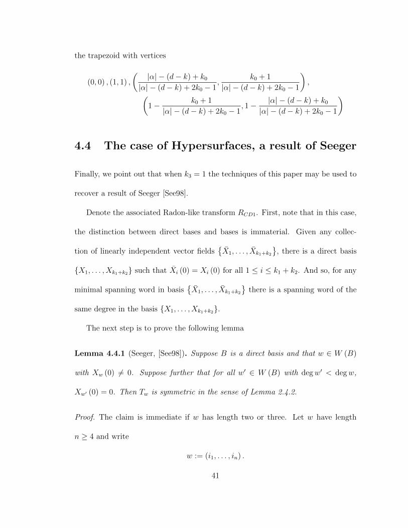
4.4 The case of Hypersurfaces, a result of Seeger

Finally, we point out that when k3 = 1 the techniques of this paper may be used to

recover a result of Seeger [See98].

Denote the associated Radon-like transform RCD1. First, note that in this case,

the distinction between direct bases and bases is immaterial. Given any collec-

tion of linearly independent vector fieldsX1, . . . , Xk1+k2

, there is a direct basis

X1, . . . , Xk1+k2 such that Xi (0) = Xi (0) for all 1 ≤ i ≤ k1 + k2. And so, for any

minimal spanning word in basisX1, . . . , Xk1+k2

there is a spanning word of the

same degree in the basis X1, . . . , Xk1+k2.

The next step is to prove the following lemma

Lemma 4.4.1 (Seeger, [See98]). Suppose B is a direct basis and that w ∈ W (B)

with Xw (0) 6= 0. Suppose further that for all w′ ∈ W (B) with degw′ < degw,

Xw′ (0) = 0. Then Tw is symmetric in the sense of Lemma 2.4.2.

Proof. The claim is immediate if w has length two or three. Let w have length

n ≥ 4 and write

w := (i1, . . . , in) .

41

For 3 ≤ k ≤ n − 1, let wk be the word wk := (i1, . . . , ik−1). Then, by the Jacobi

identity

Xw =[. . . [[Xwk

, Xik ], Xik+1] . . .], Xin

]=[. . . [[Xwk

, Xik+1], Xik ] . . .], Xin

]+[. . . [Xwk

, [Xik , Xik+1]] . . .], Xin

]If we can show that

[. . . [Xwk

, [Xik , Xik+1]] . . .], Xin

]] (0) = 0, the claim follows, since

it implies that the map is symmetric in all variables except the first two. To show

that, we prove a slightly more general statement:

If wk,1 and wk,2 are two elements of W (B) of length at least two such that

degMLwk,1 + degMLwk,2 = degML (wk, ik+1) .

then [[. . . [[Xwk,1

, Xwk,2], Xik+2

] . . .], Xin

](0) = 0. (4.4.1)

The proof proceeds by induction on k − (n− 1). In the case that k = n − 1, the

claim is immediate as (4.4.1) is a bracket of two vector fields that vanish at the

origin. If k < d− 1,

[[. . . [[Xwk,1

, Xwk,2]Xik+2

] . . .], Xin

]= −

[[. . . [[Xik+2

, Xwk,1]Xwk,2

] . . .], Xin

]−[[. . . [[Xwk,2

, Xik+2], Xwk,1

] . . .], Xin

]and (4.4.1) follows by the induction hypothesis.

Then, by Lemma 2.4.2, if w is a word associated to any basis with degw =

(d1, d2) and

(c1, c2) ∈x ∈ R2 | x > (d1 + 1, d2 + 1)

42

then RCD1 is strong type (p1, p′2), which is exactly Seeger’s result.

43

Bibliography

[Bak00] Jong-Guk Bak, An Lp-Lq estimate for Radon transforms associated to

polynomials, Duke Math. J. 101 (2000), no. 2, 259–269. MR 1738178

[CDSS17] M. Christ, S. Dendrinos, B. Stovall, and B. Street, Endpoint Lebesgue

estimates for weighted averages on polynomial curves, ArXiv e-prints

(2017).

[Cho03] Youngwoo Choi, The Lp − Lq mapping properties of convolution opera-

tors with the affine arclength measure on space curves, J. Aust. Math.

Soc. 75 (2003), no. 2, 247–261. MR 2000432

[Cho11] , Convolution estimates related to space curves, J. Inequal. Appl.

(2011), 2011:91, 6. MR 2853333

[Chr98] Michael Christ, Convolution, curvature, and combinatorics: a case

study, Internat. Math. Res. Notices (1998), no. 19, 1033–1048. MR

1654767

44

[Chr08] , Lebesgue space bounds for one-dimensional generalized radon

transforms.

[CNSW99] Michael Christ, Alexander Nagel, Elias M. Stein, and Stephen Wainger,

Singular and maximal Radon transforms: analysis and geometry, Ann.

of Math. (2) 150 (1999), no. 2, 489–577. MR 1726701

[DG91] S. W. Drury and Kang Hui Guo, Convolution estimates related to sur-

faces of half the ambient dimension, Math. Proc. Cambridge Philos.

Soc. 110 (1991), no. 1, 151–159. MR 1104610

[DLW09] Spyridon Dendrinos, Norberto Laghi, and James Wright, Universal Lp

improving for averages along polynomial curves in low dimensions, J.

Funct. Anal. 257 (2009), no. 5, 1355–1378. MR 2541272

[EO10] M. Burak Erdogan and Richard Oberlin, Estimates for the X-ray trans-

form restricted to 2-manifolds, Rev. Mat. Iberoam. 26 (2010), no. 1,

91–114. MR 2666309

[Gra14] Loukas Grafakos, Classical Fourier analysis, third ed., Graduate Texts

in Mathematics, vol. 249, Springer, New York, 2014. MR 3243734

[Gre09] Philip T. Gressman, Lp-improving properties of averages on polynomial

curves and related integral estimates, Math. Res. Lett. 16 (2009), no. 6,

971–989. MR 2576685

45

[Gre15] , Lp-nondegenerate Radon-like operators with vanishing rota-

tional curvature, Proc. Amer. Math. Soc. 143 (2015), no. 4, 1595–1604.

MR 3314072

[Gre16] P. T. Gressman, Generalized curvature for certain Radon-like operators

of intermediate dimension, ArXiv e-prints (2016).

[IS96] A. Iosevich and E. Sawyer, Sharp Lp-Lq estimates for a class of averag-

ing operators, Ann. Inst. Fourier (Grenoble) 46 (1996), no. 5, 1359–1384.

MR 1427130

[Lee04] Sanghyuk Lee, Endpoint Lp-Lq estimates for some classes of degenerate

Radon transforms in R2, Math. Res. Lett. 11 (2004), no. 1, 85–101. MR

2046202

[Lit73] Walter Littman, Lp−Lq-estimates for singular integral operators arising

from hyperbolic equations, 479–481. MR 0358443

[NSW85] Alexander Nagel, Elias M. Stein, and Stephen Wainger, Balls and met-

rics defined by vector fields. I. Basic properties, Acta Math. 155 (1985),

no. 1-2, 103–147. MR 793239

[OS82] D. M. Oberlin and E. M. Stein, Mapping properties of the Radon trans-

form, Indiana Univ. Math. J. 31 (1982), no. 5, 641–650. MR 667786

46

[PS86a] D. H. Phong and E. M. Stein, Hilbert integrals, singular integrals, and

Radon transforms. I, Acta Math. 157 (1986), no. 1-2, 99–157. MR

857680

[PS86b] , Hilbert integrals, singular integrals, and Radon transforms. II,

Invent. Math. 86 (1986), no. 1, 75–113. MR 853446

[PS91] , Radon transforms and torsion, Internat. Math. Res. Notices

(1991), no. 4, 49–60. MR 1121165

[Sec99] Silvia Secco, Fractional integration along homogeneous curves in R3,

Math. Scand. 85 (1999), no. 2, 259–270. MR 1724238

[See98] Andreas Seeger, Radon transforms and finite type conditions, J. Amer.

Math. Soc. 11 (1998), no. 4, 869–897. MR 1623430

[Sto11] Betsy Stovall, Lp improving multilinear Radon-like transforms, Rev.

Mat. Iberoam. 27 (2011), no. 3, 1059–1085. MR 2895344

[Str70] Robert S. Strichartz, Convolutions with kernels having singularities on

a sphere, Trans. Amer. Math. Soc. 148 (1970), 461–471. MR 0256219

[Str11] Brian Street, Multi-parameter Carnot-Caratheodory balls and the theo-

rem of Frobenius, Rev. Mat. Iberoam. 27 (2011), no. 2, 645–732. MR

2848534

47

[Str14] , Multi-parameter singular integrals, Annals of Mathematics

Studies, vol. 189, Princeton University Press, Princeton, NJ, 2014. MR

3241740

[TW03] Terence Tao and James Wright, Lp improving bounds for averages along

curves, J. Amer. Math. Soc. 16 (2003), no. 3, 605–638. MR 1969206

48

Reproduced with permission of copyright owner. Further reproduction prohibited without permission.