Some remarks about flows of Hilbert-Schmidt operators

HAL Id: hal-01232530https://hal.archives-ouvertes.fr/hal-01232530v2

Submitted on 24 Nov 2015

HAL is a multi-disciplinary open accessarchive for the deposit and dissemination of sci-entific research documents, whether they are pub-lished or not. The documents may come fromteaching and research institutions in France orabroad, or from public or private research centers.

L’archive ouverte pluridisciplinaire HAL, estdestinée au dépôt et à la diffusion de documentsscientifiques de niveau recherche, publiés ou non,émanant des établissements d’enseignement et derecherche français ou étrangers, des laboratoirespublics ou privés.

Some remarks about flows of Hilbert-Schmidt operatorsBenjamin Boutin, Nicolas Raymond

To cite this version:Benjamin Boutin, Nicolas Raymond. Some remarks about flows of Hilbert-Schmidt operators. Journalof Evolution Equations, Springer Verlag, 2017, 17 (2), pp.805-826. �10.1007/s00028-016-0337-3�. �hal-01232530v2�

https://hal.archives-ouvertes.fr/hal-01232530v2

https://hal.archives-ouvertes.fr

SOME REMARKS ABOUT FLOWS OFHILBERT-SCHMIDT OPERATORS

B. BOUTIN AND N. RAYMOND

Abstract. This paper deals with bracket flows of Hilbert-Schmidt operators. Weestablish elementary convergence results for such flows and discuss some of theirconsequences.

1. Introduction and results

1.1. Context. Consider a real separable Hilbert space H equipped with the Hilber-tian inner product 〈·, ·〉 and the associated norm ‖ · ‖. The set of bounded operatorsfrom H to H will be denoted by L(H) and the associated norm by ‖ · ‖. Let (en)n∈Nbe a Hilbertian basis of H and denote by D(H) the subset of bounded diagonaloperators with respect to that basis:

T ∈ D(H)⇔ ∀n ∈ N, ∃λn ∈ R, T en = λnen.

The purpose of this paper is to analyze the structural and convergence properties ofsome flows of Hilbert-Schmidt operators for whichD(H) turns out to be an attractiveHilbert-Schmidt subspace. We obtain an alternative convergence proof that appliesfor example to the flows (in infinite dimension) of Brockett, Toda and Wegner.The present paper is mainly motivated by the work by Bach and Bru [1] wherethey tackle in particular the example of the Brockett flow in infinite dimension. Weextend one of their results to a wider class of flows of Hilbert-Schmidt operators. Wemay notice here that such flows of operators have deep applications in mathematicalphysics. For instance, as recently proved by Bach and Bru in [2], they can be usedto diagonalize unbounded operators in boson quantum field theory.

This paper also aims at being a modest review of the methods and insights appear-ing in finite dimension with the idea to extend them in infinite dimension. Thesemethods are explained, for instance, in the seminal papers [6] and [3] (see also [4],and [10] for the Wegner flow), but also in the nice survey [5]. Their relations withnumerical algorithms such as the QR or LU decompositions are very deep and theidea of interpreting discrete algorithms as samplings of continuous flows has now along story (see, for instance, [7, 8] and [9]). Commenting this idea would lead us farbeyond the scope of this paper, but we will briefly discuss it when describing ournumerical illustrations.

1.2. Results. Let us now describe the results of this paper. For that purpose, weintroduce some general notations.

Notation 1.1. Below are the notations that we will constantly use in the paper.

1

2 B. BOUTIN AND N. RAYMOND

(a) We denote L2(H) the set of the Hilbert-Schmidt operators on H and the associ-ated norm is ‖ · ‖HS. In other words, H ∈ L2(H) means that, for any Hilbertianbasis (en)n∈N, we have ∑

n≥0

‖Hen‖2 < +∞ ,

and this last quantity is independent from the Hilbert basis and is denoted by‖H‖2

HS and we have ‖H‖ ≤ ‖H‖HS. We also recall that the Hilbert-Schmidtoperators are compact and that, if (λn(H))n∈N is the non-increasing sequence ofthe eigenvalues of H, we have

‖H‖2HS =

+∞∑n=0

|λn(H)|2 .

(b) We will denote by S(H), A(H) and U(H) the sets of the bounded symmetric,bounded skew-symmetric and unitary operators respectively. We also introduceS2(H) = S(H) ∩ L2(H) and A2(H) = A(H) ∩ L2(H). They are Hilbert spacesequipped with the scalar product (A,B) 7→ Tr(A?B).

(c) In the sequel we will use a fixed Hilbert basis (en)n∈N and for any H ∈ L2(H)and any integers i, j ∈ N, we will denote hi,j(t) = 〈H(t)ei, ej〉.

1.2.1. An elementary convergence result. We will consider infinite systems deter-mined by matrices that are balanced in the sense of the following definition.

Definition 1.2. A family of real-valued functions (gi,j)i,j∈N defined on R is said tobe balanced if

∀i, j ∈ N, ∃ci,j ∈ L∞(R,R+), ∀t ∈ R, |gi,j(t)| ≤ ci,j(t)|gj,i(t)| .It is said to be pointwise bounded if, for all t ∈ R, sup

i,j|gi,j(t)| < +∞.

Let us now state one of the main results of this paper. It is a general convergenceresult for infinite systems of differential equations. As we will see, many differentclassical situations may be reduced to this result.

Theorem 1.3. Consider H ∈ C1(R,L2(H)) such that

i) the function t 7→ ‖H(t)‖HS is bounded,ii) the family (hi,j)i,j∈N is balanced,iii) there exists a pointwise bounded and balanced family of measurable functions

(gi,j)i,j∈N defined on R such that

(1.1) ∀t ∈ R, h′i,i(t) =+∞∑j=0

gi,j(t)|hi,j(t)|2 .

Suppose that there exists T > 0 and a sign sequence (ε`)`∈N ∈ {−1, 1}N, such that

(1.2) ∀t ≥ T, ∀k, ` ∈ N, k ≥ `, ε`g`,k(t) ≥ 0 .

Then we have the integrability property

(1.3) ∀` ∈ N,+∞∑j=0

∫ +∞

T

|g`,j(t)||h`,j(t)|2 dt < +∞ ,

SOME REMARKS ABOUT FLOWS OF HILBERT-SCHMIDT OPERATORS 3

and any diagonal term h`,`(t) converges at infinity to a real value denoted by h`,`(∞).

Under the additional semi-uniform lower bound condition

(1.4) ∀` ∈ N, ∃c` > 0, ∀j 6= `, ∀t ≥ T, |g`,j(t)| ≥ c` ,

we have

(1.5)∑j 6=`

∫ +∞

T

|h`,j(t)|2 dt =

∫ +∞

T

‖H(t)e` − h`,`(t)e`‖2 dt < +∞ .

Suppose moreover that, for any ` ∈ N, the function t 7→ ‖H ′(t)e`‖ is bounded, thenfor any ` ∈ N, H(t)e` converges to h`,`(∞)e`.

Remark 1.4. Theorem 1.3 remains true if, instead of the assumption (1.2), we onlyassume that there exists a one-to-one integer mapping function φ : N → N, a timeT > 0 and a sign sequence ε` ∈ {−1, 1} (` ∈ N) such that

∀t ≥ T, ∀k ∈ N, k /∈ {φ(i), 0 ≤ i ≤ `− 1}, ε`gφ(`),k(t) ≥ 0 .

We will apply Theorem 1.3 to “bracket” flows. Let us state a proposition thatdescribes the fundamental property of such flows.

Proposition 1.5. Let G : S(H)→ A(H) be a locally Lipschitzian function and letus consider the following Cauchy problem

(1.6) H ′ = [H,G(H)] , t ≥ 0 , H(0) = H0 ∈ S2(H) .

There exists a unique global solution H ∈ C1([0,+∞),S2(H)) unitarily equivalent tothe initial data H0. More precisely there exists U ∈ C1([0,+∞),U(H)) such that forany t ≥ 0 one has H(t) = U(t)?H0U(t).

Let us now provide two corollaries of Theorem 1.3.

First let us introduce two convenient definitions.

Definition 1.6. Given a Hilbertian basis (en)n∈N, we introduce

i. the symmetric family of symmetric Hilbert-Schmidt operators (Ei,j)(i,j)∈N2 de-fined by

Ei,j(·) =

{1√2(e∗j(·)ei + e∗i (·)ej) if i 6= j

e∗i (·)ei if i = j.

ii. the skew-symmetric family of skew-symmetric Hilbert-Schmidt operators (E±i,j)(i,j)∈N2

defined by

E±i,j(·) =1√2

(e∗j(·)ei − e∗i (·)ej) .

Since the families (Ei,j)i≤j and (E±i,j)i<j are Hilbertian bases of S2(H) and A2(H)respectively, this motivates the following definition.

Definition 1.7. We say that G ∈ L (S2(H),A2(H)) is diagonalizable when thereexists a Hilbertian basis (en)n∈N and a skew-symmetric family (gi,j) such that

G(Ei,j) = gi,jE±i,j .

In this case, we say that (gi,j) is the matrix-eigenvalue of G. Note that the matrix-eigenvalue of G is balanced and pointwise bounded (G is bounded).


Corollary 1.8. Let G ∈ L (S2(H),A2(H)) be a diagonalizable map such that itsmatrix-eigenvalue satisfies (1.2) and (1.4). Then the Cauchy problem (1.6) admitsa unique global solution H ∈ C1([0,+∞),S2(H)) which weakly converges in S2(H)to a diagonal Hilbert-Schmidt operator H∞. Moreover, if α is a diagonal term ofH∞ with multiplicity m, then α is an eigenvalue of H0 of multiplicity at least m.

Then we can apply our theorem to the finite dimensional case and even get anexplicit convergence rate. Note that this presentation does not involves a Lyapunovfunction and relies on the a priori convergence of H(t). This is a way to avoid, as faras possible, the considerations related to the evolution of the corresponding unitarymatrices (U(t))t≥0 in U(H) (that is not compact in infinite dimension).

Corollary 1.9. Consider a finite dimensional Hilbert space H of dimension d. Un-der the assumptions of Corollary 1.8, the solution of (1.6) converges to a diagonaloperator H∞ = diag (α`)0≤`≤d−1 in L(H) and the α` are exactly the eigenvalues (withmultiplicity) of H0. If, in addition, the eigenvalues of H0 are simple, then there existT,C > 0 such that, for all t ≥ T , we have

‖H(t)−H∞‖ ≤ Ce−γt ,

where γ = infT −|gi,j(αi − αj)| > 0 with

T − = {(i, j) ∈ {0, . . . , d− 1}2 : i < j and gi,j(αi − αj) < 0} .

Note that, in Corollary 1.9, we have not to exclude special initial conditions to getan exponential convergence (see [4, Theorem 3]).

The following proposition states that, even in infinite dimension, we may find expo-nentially fast eigenvalues of a generic Hilbert-Schmidt operator thanks to a bracketflow. Note that, in this case, we get a stronger convergence as the one established byBach and Bru in [1, Theorem 7] for the Brockett flow and that we may also considernon symmetric operators.

Proposition 1.10. Assume that H0 ∈ L2(H) (not necessarily symmetric) is diago-nalizable with eigenvalues (λj)j≥1 with decreasing real parts. Let us also assume thatwe may find P ∈ L(H) such that PH0P

−1 = Λ where Λ = diag(λj)j∈N is a diagonaloperator and such that the minors of P , PJ = (〈Pei, ej〉)0≤i,j≤J are invertible for allJ ∈ N.

We use the choice

G(H) = H− − (H−)? .

Then, we have, for all ` ∈ N,

H(t)e` −+∞∑j=`+1

〈H(t)e`, ej〉ej = λè` +O(e−tδ`

), δ` = min

0≤j≤`<(λj − λj+1) .

Note in particular that, in the symmetric case, H(t) converges to a diagonal operatorH∞ that has exactly the same eigenvalues as H0 (even in infinite dimension). Thisproperty is slightly stronger than the last one stated in Corollary 1.8: for the Todaflow, in infinite dimension, no eigenvalue is lost in the limit.


1.2.2. Organization of the paper. Section 2 is devoted to the proof of Theorem 1.3,Proposition 1.5 and Corollary 1.8. We also provide examples of applications of ourresults (to the Brockett, Toda and Wegner flows) in infinite dimension. In Section3, we discuss the case of finite dimension to the light of our results and discuss theexponential convergence of the flows (Corollary 1.9 and Proposition 1.10).

2. Existence and global convergence results

2.1. Proof of the main theorem. This section is devoted to the proof of Theo-rem 1.3. We start by stating two elementary lemmas.

Lemma 2.1. Consider h ∈ C1(R+) a real-valued bounded function, F ∈ L1(R+) andG a nonnegative measurable function defined on R+ such that

∀t ≥ 0, h′(t) = F (t) +G(t).

Then, the function G is integrable and h converges to a finite limit at infinity.

Proof. Observe that, due to the sign of G, one gets for all x ≥ 0∫ x

0

|G(t)| dt =

∫ x

0

G(t) dt = h(x)− h(0)−∫ x

0

F (t) dt ≤ 2 supR+

|h|+∫ +∞

0

|F (t)| dt .

Therefore G is integrable and, for all x ≥ 0

h(x) = h(0) +

∫ x

0

(F (t) +G(t)) dt ,

which converges as x tend to infinity. �

Lemma 2.2. Let w be a function defined on R+ with nonnegative values. Supposethat w is Lipschitz continuous with Lipschitz constant C > 0. Then, for any x ≥ 0,one has

w(x)2 ≤ 2C

∫ +∞

x

w(y) dy ≤ +∞.

Suppose moreover that w is integrable, then limx→+∞

w(x) = 0.

Proof. Since w is Lipschitzian, we have, for all x, y ∈ R,

w(x) ≤ C|x− y|+ w(y) ,

so that, integrating with respect to y between x and x+ w(x)C

, we get

w(x)2

C≤ w(x)2

2C+

∫ x+w(x)C

x

w(y) dy ,

and the conclusion follows. �

We can now complete the proof of Theorem 1.3.


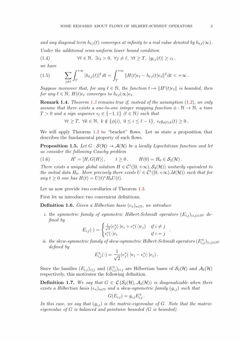
2.1.1. Convergence. Consider first Equation (1.1) with i = 0. Thanks to the signproperty (1.2) we have

ε0h′0,0(t) =

∑j∈N

|g0,j(t)||h0,j(t)|2 .

The boundedness of t 7→ ‖H(t)‖HS implies the boundedness of t 7→ h0,0(t) andthus Lemma 2.1 implies the existence of a finite limit h0,0(∞) and the integrabilityproperty ∫ +∞

T

∑j∈N

|g0,j(t)||h0,j(t)|2 dt < +∞ .

Then, the rest of the proof is by induction on ` ∈ N. Let ` ≥ 1 be an integer andassume that, for any integers 0 ≤ k ≤ `− 1, we have∫ +∞

T

∑j∈N

|gk,j(t)||hk,j(t)|2 dt < +∞ .

Equation (1.1) with i = ` and the sign assumption (1.2) give

ε`h′`,`(t) =

∑k≤`−1

ε`g`,k(t)|h`,k(t)|2 +∑j≥`

|g`,j(t)||h`,j(t)|2 .

Again, t 7→ h`,`(t) is bounded. Let us now prove the integrability of the first sumin the right hand side. Since the families (gi,j) and (hi,j) are balanced, we get thefollowing

∃C` ≥ 0, ∀t ≥ T, ∀k ≤ `− 1, |g`,k(t)||h`,k(t)|2 ≤ C`|gk,`(t)||hk,`(t)|2.

Therefore we have(2.1)∫ +∞

T

∑k≤`−1

|g`,k(t)||h`,k(t)|2 dt ≤ C`∑k≤`−1

∫ +∞

T

|gk,`(t)||hk,`(t)|2 dt

≤ C`∑k≤`−1

∫ +∞

T

∑j∈N

|gk,j(t)||hk,j(t)|2 dt < +∞ .

Finally, Lemma 2.1 applies and we get the existence of a finite limit h`,`(∞) togetherwith the integrability property:∫ +∞

T

∑j≥`

|g`,j(t)||h`,j(t)|2 dt < +∞ ,

and then, thanks to (2.1), we find∫ +∞

T

∑j∈N

|g`,j(t)||h`,j(t)|2 dt < +∞ .

This ends the proof of the integrability property and of the convergence of diagonalterms.


2.1.2. Stronger convergence. Consider now the additional assumption (1.4). For anyfixed ` ∈ N, we have∑

j 6=`

∫ +∞

T

|h`,j(t)|2 dt ≤ 1

c`

∑j 6=`

∫ +∞

T

|g`,j(t)||h`,j(t)|2 dt < +∞ .

For any t ≥ T , we let

w`(t) =∑j 6=`

|h`,j(t)|2 dt = ‖K`(t)‖2 with K`(t) = H(t)e` − h`,`(t)e` .

For t ≥ s ≥ T , the Cauchy-Schwarz inequality implies that

|w`(t)− w`(s)| ≤ ‖K`(t)−K`(s)‖‖K`(t) +K`(s)‖ .On one hand, we have

‖K`(t) +K`(s)‖ ≤ 2 supσ≥T‖H(σ)‖HS.

On the other hand, we write

‖K`(t)−K`(s)‖ ≤ ‖H(t)e` −H(s)e`‖+ |h`,`(t)− h`,`(s)|

≤∫ t

s

‖H ′(σ)e`‖ dσ +

∫ t

s

|h′`,`(σ)| dσ

≤ 2

∫ t

s

‖H ′(σ)e`‖ dσ ≤ 2M |t− s| ,

where M is a uniform bound of t 7→ ‖H ′(t)e`‖. Finally, w` is a nonnegative and Lip-schitz continuous function, which is moreover integrable thanks to (1.5). ThereforeLemma 2.2 implies that w`(t) goes to 0 as t goes to +∞.

2.2. Proof of Proposition 1.5.

2.2.1. Local existence. Let us introduce the function F : S(H)→ S(H) defined by

(2.2) ∀H ∈ S(H) , F (H) = [H,G(H)] .

Note indeed that, for all H ∈ S(H), by using that G is valued in A(H), we have

F (H)? = (HG(H)−G(H)H)? = G(H)?H? −H?G(H)? = F (H) .

Moreover F is locally Lipschitzian sinceG is. By using the Cauchy-Lipschitz theoremin the Banach space (S(H), ‖ · ‖) with the function F , we get the local existence ofa solution of the Cauchy problem (1.6), on a maximal time interval [0, Tmax), withTmax > 0.

2.2.2. Global existence. Let us now show that Tmax = +∞ and that, we have, for allt ∈ [0,+∞), H(t) ∈ L2(H) and ‖H(t)‖HS = ‖H0‖HS. Let us consider the followingCauchy problem:

(2.3) U ′ = UG(H) , U(0) = Id ,

where H is the local solution of (1.6) on [0, Tmax). Since the equation is linear,we know that there exists a unique solution U defined on [0, Tmax). By using thatG(H(t)) ∈ A(H), it is easy to check that, on [0, Tmax), we have U?U = UU? = Id.


Then an easy computation shows that the derivative of t 7→ U(t)H(t)U(t)? is zeroand thus

∀t ∈ [0, Tmax) , H(t) = U(t)?H0U(t) .

From this, we infer that, for all t ∈ [0, Tmax), H(t) ∈ L2(H) and ‖H(t)‖HS = ‖H0‖HS.Therefore, on [0, Tmax), the function H is bounded in L2(H) ⊂ L(H). Thus we getTmax = +∞.

2.2.3. Linear case. Let us now discuss the proof of Corollary 1.8. First we noticethat, since L2(H) is an ideal of L(H), the function F defined in (2.2) sends theHilbert space S2(H) into itself. Thus, we may apply the Cauchy-Lipschitz theoremin this space and the global existence is ensured by the investigation in the previoussection. Let us reformulate (1.6) in the Hilbert basis (en)n∈N. We easily have

h′i,i(t) = 2〈G(H(t))ei, H(t)ei〉 .

Then we notice that

H(t) =∑k≤`

hk,`(t)Ek,` , G(H(t)) =∑k<`

gk,`hk,`(t)E±k,` .

We get

H(t)ei =+∞∑j=0

hi,j(t)ej , G(H(t))ei = −∞∑j=0

gi,jhi,j(t)ej ,

and thus

h′i,i(t) = −2+∞∑j=0

gi,j|hi,j(t)|2 .

Moreover we notice that

‖H ′(t)‖ ≤ 2‖H(t)‖‖G(H(t))‖ ≤ 2‖G‖‖H(t)‖2HS = 2‖G‖‖H0‖2

HS .

Therefore, thanks to the assumptions on (gi,j), we may apply Theorem 1.3.

Then we let α` = h`,`(+∞) and we notice that

+∞∑`=0

‖H(t)e`‖2 = ‖H(t)‖2HS = ‖H0‖2

HS ,

and thus, with the Fatou lemma, we get

sup`∈N|α`|2 ≤

+∞∑`=0

α2` ≤ lim inf

t→+∞‖H(t)‖2

HS = ‖H0‖2HS .

We introduce the Hilbert-Schmidt operator H∞ := diag (α`) defined by

∀x ∈ H , H∞(x) =+∞∑`=0

α`xè` , where x =+∞∑`=0

xè` .

In particular, we get that, for all ` ∈ N, H(t)e` converges to H∞e`. Let us now

consider x ∈ H and ε > 0. There exists L ∈ N such that ‖x−L∑`=0

xè`‖ ≤ ε. Since


‖H(t)‖ ≤ ‖H(t)‖HS = ‖H0‖HS and ‖H∞‖ ≤ ‖H0‖HS, we get that, for all t ≥ 0,

‖(H(t)−H∞)x‖ ≤ ‖(H(t)−H∞)L∑`=0

xè`‖+ 2ε‖H0‖HS ,

and, for t large enough, it follows that

‖(H(t)−H∞)x‖ ≤ 2ε‖H0‖HS + ε .

Therefore H(t) strongly converges to H∞ and thus H(t) weakly converges to H∞ inS2(H).

Let us consider an eigenvalue α of H∞, with multiplicity m and associated with theeigenvectors e`1 , . . . , e`m . Then, for all ε > 0, there exists T > 0 such that, for allj ∈ {1, . . . ,m},

‖H(T )e`j − αe`j‖ ≤ ε .

or equivalently‖H0fj − αfj‖ ≤ ε , with fj = U(T )e`j .

Therefore, the spectral theorem implies that

∀ε > 0 , range(1[α−ε,α+ε](H0)

)≥ m.

This proves that α is an eigenvalue of H0 with multiplicity at least m.

2.3. Examples. Let us now provide examples of applications of our convergenceresults.

2.3.1. Brockett’s choice. For a given A = diag(a`) ∈ D(H) with a non-increasingsequence (a`)`∈N ∈ RN

+, we take G1(H) = [H,A]. Since L2(H) is an ideal of L(H),we have G1 : S2(H) → A2(H) and ‖G1‖ ≤ 2‖A‖. Moreover G1 is diagonalizableand gi,j = aj − ai.

2.3.2. Toda’s choice. If H ∈ S2(H), we introduce

H− =∑

1≤i≤j

hi,je∗i ej and G2(H) = H− − (H−)? .

By definition, we have G2 : S2(H) → A2(H) and ‖G‖ ≤ 2‖H−‖ ≤ 2‖H‖HS. Inaddition, G2 is diagonalizable with gi,j = −1 for i < j.

2.3.3. Wegner’s choice. Let us finally discuss a non-linear example. We takeG3(H) =[H, diag(H)]. Since G3 sends the symmetric operators in the skew symmetric op-erators, we get that G3 generates a flow that preserves the Hilbert-Schmidt norm.Thus the flow is global. Explicitly we have H ′ = [H, [H, diagH]]. In particular, weget

h′i,i(t) = 2+∞∑j=0

(hi,i(t)− hj,j(t))|hij(t)|2 .

If, for large times, the diagonal terms become distinct (in the sense of (1.2) and(1.4)), then, by Theorem 1.3, H(t) converges to a diagonal matrix H∞. Actually, inthis case, the convergence is exponential in finite dimension (see Section 3.1.3 wherethe linearization of the same kind of system is explained).


3. Exponential convergence

3.1. A stronger convergence in finite dimension. This section is devoted tothe proof of Corollary 1.9.

3.1.1. Reminder of the stable manifold theorem. Let us recall a classical theorem.

Theorem 3.1. Consider F ∈ C1(Rd,Rd) such that F (0) = 0 and the differentialdF0 is diagonalizable with no eigenvalues with zero real parts. Denote E− and E+

respectively the stable and unstable subspaces of dF0 and k = dim(E−) so that d−k =dim(E+). Let us consider the following Cauchy problem

(3.1) H ′(t) = F (H(t)) , t ∈ R , H(0) = H0 ,

and suppose, for any H0 ∈ Rd, there exists a unique global solution H ∈ C1(R,Rd).

Then there exists V a neighborhood of 0 in Rd and two C1-manifolds in V, sayW− and W+, with respective dimensions k and d − k, tangent at 0 to E− and E+

respectively, and such that for all H0 ∈ V, the solution of (3.1) satisfies:

(a) limt→+∞H(t) = 0⇔ H0 ∈ W−,(b) limt→−∞H(t) = 0⇔ H0 ∈ W+.

More precisely, the manifold W− (stable at +∞) is the graph of a C1-map denotedϕ− defined over E− ∩ V and satisfying ϕ−(0) = 0 et dϕ−(0) = 0. The same resultholds for W+.

The above result is a classical consequence of a fixed point argument and the con-vergence to such hyperbolic equilibrium point is exponential in the stable manifold,with a convergence rate similar to the one of the linearized Cauchy problem in thetangent space E−, i.e. of order at worst O(e−γt) where

−γ = max ({<(sp(dF0))} ∩ R−) < 0 .

3.1.2. Convergence to the diagonal matrices: a naive estimate. From Corollary 1.8,we know that H(t) converges to H∞ = diag(α`) where the α` are exactly the eigen-values of H0 sinceH is of finite dimension. This convergence analysis is then reducedto a small neighborhood of H∞. The differential equation reads

H ′ = F (H) , F (H) = [H,G(H)] ,

and, since G and H∞ are diagonal in the canonical bases, we have G(H∞) = 0. Wededuce that the differential of F at H∞ is given by

∀H ∈ S(H) , dFH∞(H) = [H∞, G(H)] .

Thus dFH∞ is an endomorphism of the space of symmetric matrices and it is diago-nalized in the basis Ei,j since a straightforward computation gives

dFH∞(Ei,j) = gi,j(αi − αj)Ei,j .

Since 0 is an eigenvalue of dFH∞ of multiplicity d, we cannot directly apply the stablemanifold theorem. Nevertheless, we can elementarily get the following proposition.


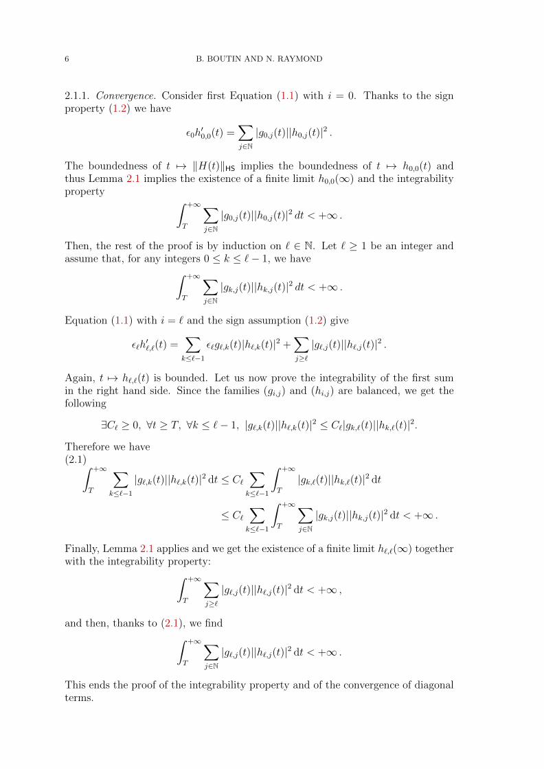
Proposition 3.2. Let us introduce

T = {(i, j) ∈ {0, . . . , d− 1}2 : i < j} ,

and assume that

−γ := maxT

gi,j(αi − αj) < 0 .

Then, for all ε > 0, there exist T,C > 0 such that, for all t ≥ T ,

‖H(t)− diag(H(t))‖HS ≤ Ce−γt .

Proof. Let us define

R(H) = F (H)− F (H∞)− dFH∞(H −H∞) = [H −H∞, G(H − diag(H))] ,

and

∆(t) = H(t)− diag(H(t)) .

Let us now consider ε > 0 and T > 0 such that, for all t ≥ T , we have

‖H(t)−H∞‖HS ≤ ε , ‖R(H(t))‖HS ≤ 2ε‖G‖‖∆(t)‖HS .

For all H ∈ S(H), we notice that diag (dFH∞(H)) is zero. Therefore we have

∆′(t) = dFH∞(∆(t)) +R(H(t))− diag (R(H(t))) .

The Duhamel formula reads, for t ≥ T ,

∆(t) = e(t−T )dFH∞∆(T ) +

∫ t

T

e(t−s)dFH∞{R(H(s))− diag (R(H(s)))} ds ,

where ∆ and R(H) − diag (R(H)) ∈ Span (Ei,j)i<j. Since (Ei,j) is orthonormalizedfor the HS-norm, we deduce that

‖∆(t)‖HS ≤ e−γ(t−T )‖∆(T )‖HS +

∫ t

T

e−(t−s)γ‖R(H(s))− diag (R(H(s))) ‖HS ds ,

so that

eγt‖∆(t)‖HS ≤ eγT‖∆(T )‖HS + 2ε‖G‖∫ t

T

esγ‖∆(s)‖HS ds .

From the Gronwall lemma, we get, for t ≥ T ,

eγt‖∆(t)‖HS ≤ eγT‖∆(T )‖HSe2ε‖G‖(t−T ) ,

and thus

‖∆(t)‖HS ≤ e(−γ+2ε‖G‖)(t−T )‖∆(T )‖HS .We deduce that the same convergence holds for the diagonal terms.

Let us now eliminate the dependence in ε in the exponential. We easily have

H ′(t) = F (H(t)) = [H(t), G(H(t))] = [H(t), G(∆(t))] ,

so that for all t ≥ T

‖H ′(t)‖HS ≤ 2‖G‖‖H0‖HS‖∆(t)‖HS ≤ 2‖G‖‖H0‖HSCe(−γ+ε)t .

It follows that

‖H(t)−H∞‖HS ≤∫ +∞

t

‖H ′(s)‖HS ds ≤ 2‖G‖‖H0‖HSC

−γ + εe(−γ+ε)t .


We get therefore the existence of a constant D that depends on ε and ‖H0‖HS onlysuch that for all t ≥ T ,

‖H(t)−H∞‖HS ≤ De(−γ+ε)t .

Coming back to the previous proof with De(−γ+ε)t in place of ε, we get then fromthe Gronwall lemma

eγt‖∆(t)‖HS ≤ eγT‖∆(T )‖HSe2D‖G‖∫ tT e

(−γ+ε)s ds ,

that may be bounded independently from t ≥ T . Therefore we may omit the ε termin exponential convergence rate.

�

Remark 3.3. In particular, this proposition may be used as follows. Let us considerε such that 0 < ε < inf

T|αi − αj| and assume that ‖H0 − H∞‖HS < ε which may be

insured by using the flow up to the time T . Then, there exists a permutation Π suchthat

‖H0 − H∞‖HS = O(ε) , H0 = Π?H0Π , H∞ = diag(α`) ,

where (α`)`∈{0,...,d} denotes the sequence of the eigenvalues of H0 in the opposite orderwith respect to gi,j. Then we have

‖H(t)− diag(H(t))‖HS ≤ Ce−γt .

In other words, up to a permutation and as soon as we are close enough to the limit,we can insure an exponential convergence (with rate γ) to the diagonal matrices.

3.1.3. Proof of Corollary 1.9. It is actually more convenient to work on the side ofthe unitary transform U . We recall that, from (2.3), U satisfies

U ′ = UG(U?H0U) = F(U) .

Let us first notice that U converges.

Proposition 3.4. The function t 7→ U(t) converges as t tends to +∞. Moreover,the limit U∞ belongs to the finite set

{Π?diag(ε`)Π , Π ∈ Sn , ε` ∈ {±1}} .

Proof. The orthogonal group is compact since the dimension is finite. If U convergesto U∞, then U∞ is still unitary and H∞ = U?

∞H0U∞. There exists an orthogonaltransformation Q0 such that Q0H0Q

?0 = diag(α`) where the α` are in non-increasing

order. Thus, there exists a permutation Π such that

H∞ = (U?∞Q

?0Π?)H∞(ΠQ0U∞) ,

Thus, since H∞ is diagonal with simple coefficients, ΠQ0U∞ is itself diagonal andthus, we get (ΠQ0U∞)2 = Id.

Now we know that H(t) tends to H∞ so that U ′(t) goes to 0 as t goes to +∞. Sincethe orthogonal group is compact and that F is continuous with a finite number ofzeros, we deduce that U must converge to a zero of F . �


We can notice that the proof of Proposition 3.4 relies on the convergence of H(t)when t goes to +∞. Without this a priori convergence, we would not get theconvergence of U(t) for any given H0. As in [4, Theorem 3], one should excludefrom the initial conditions the union of the stable manifolds of all the stationarypoints that are not attractive. With the compactness of U(H), this would imply theconvergence of U(t) towards the (unique) attractive point. Actually such restrictionson the initial conditions are not necessary to get the convergence as explained in thefollowing lines.

Let us now parametrize, locally near U∞, the orthogonal group U(H) by its Lie alge-bra A(H). By the local inversion theorem, it is well known that exp : A(H)→ U(H)is a local smooth diffeomorphism between a neighborhood of 0 and a neighborhoodof Id. We recall that

(d exp(A))−1(H) = exp(−A)+∞∑k=0

(adA)k

(k + 1)!H .

For t ≥ T , we may write U(t) = U∞ exp(A(t)). Thus we have

U ′ = U∞eA(t)G(e−A(t)H∞e

A(t)) .

We get

A′(t) = eA(t)G(e−A(t)H∞eA(t))e−A(t) +R1(t) ,

with R1(t) = O(‖A(t)‖2). We infer that

A′(t) = G([H∞, A]) +R2(t) ,

with R2(t) = O(‖A(t)‖2). Now A 7→ G([H∞, A]) is an endomorphism of the space ofskew-symmetric matricesA(H) and it is diagonalized in the basis E±i,j with i < j witheigenvalues gi,j(αi−αj). By assumption these eigenvalues are not zero. We may ap-ply the stable manifold theorem. Since A(t) goes to 0, this means, by definition, thatA(t) belongs to the stable manifold near 0. Therefore it goes exponentially to zero,with a convergence rate a priori of order O(e−γt), with γ = inf

T −|gi,j(αi − αj)| > 0.

Of course, the convergence may be stronger, depending on the stable manifold onwhich A(t) is evolving. Then H(t) inherits this convergence rate.

3.2. Abstract factorization of Hilbert-Schmidt operators. Actually it is pos-sible to get a quantitative convergence to the eigenvalues of non self-adjoint operatorsin infinite dimension. Note that, in Theorem 1.3, we do not have such a quantifica-tion, even for symmetric operators.

3.2.1. Chu-Norris decomposition for Hilbert-Schmidt operators. Let us consider anapplication G : L(H)→ A(H) of class C1 and the following Cauchy problem:

H ′(t) = [H(t), G(H(t))] , H(0) = H0 ∈ L2(H) .

We also introduce the equations

g′1(t) = g1(t)G(H(t)) , g1(0) = Id ,

g′2(t) = (H(t)−G(H(t)))g2(t) , g2(0) = Id .

Then we have the following lemma (coming from a straightforward adaptation ofthe theorems in [6] that are actually true for bounded operators).


Lemma 3.5. The solutions H, g1 and g2 are global and of class C1. Then, we haveg1 ∈ C1(R,U(H)) and

(3.2) H(t) = g1(t)−1H0g1(t) = g2(t)H0g−12 (t)

and thus we have H ∈ C1(R,L2(H)).

Moreover we have the relations

(3.3) etH0 = g1(t)g2(t) , etH(t) = g2(t)g1(t) .

Proof. Let us just give some insights of the proof. By easy calculations, we get(g1g

?1)′ = 0, (g1Hg

?1)′ = 0, and (g−1

2 Hg2)′ = 0, which ensures both the first algebraicproperties and the global character of the solutions in the considered spaces. Thefirst exponential factorization follows from the uniqueness result for the followingCauchy problem

Z ′(t) = H0Z(t), t ∈ R, Z(0) = Id ,

of which both etH0 and g1(t)g2(t) are solutions. The second exponential factorizationthen easily follows as a consequence. �

3.2.2. Proof of Proposition 1.10. It is easy to see that

g2(t)e` =∑j=0

α`,j(t)ej .

Thus we may write

etH0e` =∑j=0

α`,j(t)g1(t)ej .

We get

P−1etΛf` =∑j=0

α`,j(t)g1(t)ej , f` = Pe` .

We have

(3.4)∑j=0

α`,j(t)g1(t)ej = P−1etΛf` =J∑j=0

p`,jetλjvj +

+∞∑j=J+1

p`,jetλjvj ,

where vj = P−1ej. We may also write

(3.5) AJ

e0...eJ

= PJetΛJ

g?1v0...

g?1vJ

+O(et<(λJ+1)) .

and

AJ = PJetΛJ

g?1v0...

g?1vJ

[e0 . . . eJ ] +O(et<(λJ+1)) .

By using the simplicity of the eigenvalues, we get, by using a Neumann series and thefact that PJ is invertible, that AJ is invertible when t is large enough. In addition,we get

(3.6) ‖A−1J ‖ = O

(e−t<(λJ )

).


From (3.4), we get

∑j=0

α`,j(t)H0g1(t)ej =J∑j=0

p`,jλjetλjvj +O

(et<(λJ+1)

),

so that, with (3.2),

∑j=0

α`,j(t)g1(t)H(t)ej =J∑j=0

p`,jλjetλjvj +O

(et<(λJ+1)

),

which may be written as

AJ

H(t)e0...

H(t)eJ

= PJΛJetΛJ

g?1v0...

g?1vJ

+O(et<(λJ+1)) .

or, with (3.6), H(t)e0...

H(t)eJ

= A−1J PJΛJe

tΛJ

g?1v0...

g?1vJ

+O(et<(λJ+1−λJ )) .

From (3.5), we get

(3.7)

g?1v0...

g?1vJ

= e−tΛJP−1J AJ

e0...eJ

+O(et<(λJ+1−λJ )) ,

and thus

(3.8)

H(t)e0...

H(t)eJ

= A−1J PJΛJP

−1J AJ

e0...eJ

+O(et<(λJ+1−λJ )) .

Therefore the space spanned by e0, . . . , eJ is invariant by H(t) up to an error oforder O(et<(λJ+1−λJ )). In view of (3.8), we get the conclusion by induction on J ≥ 0.In other words, we approximate the diagonal terms of H(t) one by one by movingJ from 0 to +∞.

3.3. Numerics. In the following numerical illustrations, we consider the finite di-mensional example of flows evolving in matrices ofMd(R) with d = 5. As an initialdata, let fix H0 = Q diag(`2)1≤`≤dQ

?, where Q = exp(B5) is a unitary matrix definedthrough the following choice of Bd ∈ Ad(R) skew-symmetric:

Bd = (bi,j), bi,j = 1, for i > j .

The numerical solver to compute any of the below approximate solutions is an adap-tive 4th-order Runge-Kutta scheme.


Figure 1. Brockett flow – Convergence of diagonal entries (left),exponential convergence of H(t) (right).

3.3.1. Brockett’s choice. The considered Brockett’s bracket flow is given by thechoice A = diag(d−`)0≤`≤d−1 ∈ D(Rd) with non-increasing diagonal elements. Withthese data, we observe the convergence to the limit H∞ = diag([25, 16, 9, 4, 1]), seeFigure 1. The diagonal terms are sorted in a descending order, according to thecoefficients in A. The effective exponential rate of convergence γ = 3 coincides, forsufficiently large times, with the worst expected one (Corollary 1.9). The matrix ofgi,j(αi − αj) is there:

0 −9 −32 −63 −96−9 0 −7 −24 −45−32 −7 0 −5 −16−63 −24 −5 0 −3−96 −45 −16 −3 0

.

Let change the initial data to the following one H0 = Q diag(`2)1≤`≤d Q?, where

Q =

(1 (0)

(0) exp(B4)

). Then H0 takes the above block form

(3.9)

(1 (0)

(0) K

),

where K ∈ S4(R) has spectrum {4, 9, 16, 25}. Then we observe the convergence tothe limit H∞ = diag([1, 25, 16, 9, 4]), with an exponential rate γ = 5. Namely, thematrix of gi,j(αi − αj) is then:

0 24 30 24 1224 0 −9 −32 −6330 −9 0 −7 −2424 −32 −7 0 −512 −63 −24 −5 0

.

In fact, in that case the exact flow evolves in the linear subspace described in (3.9)and the positive coefficients of the above matrix concern precisely the evolution ofthe flow transversally to that subspace. It is only because of the very specific form ofthe initial data that the numerical flow evolves in the same way, elsewhere numerical


Figure 2. Toda flow – Convergence of diagonal entries (left), expo-nential convergence of H(t) (right).

Figure 3. Toda flow – Convergence of extradiagonal entries.

error due to the finite precision would have induced a convergence of the numericalsolution to the totally sorted limit with rate γ = 3.

3.3.2. Toda’s choice. For the same test case, the Toda flow gives similar results, seeFigure 2. Once again, the effective exponential rate of convergence is γ = 3 andcoincides, for sufficiently large times with the theoretical one. Actually the matrixof gi,j(αi − αj) is there:

0 −9 −16 −21 −24−9 0 −7 −12 −15−16 −7 0 −5 −8−21 −12 −5 0 −3−24 −15 −8 −3 0

.

On Figure 3, we present the numerical counterpart of Proposition 1.10. For any1 ≤ ` ≤ d−1, we compute the norm of the residual column ‖(hj,`−α`δj,`)`≤j≤d‖ alongthe time. The thick dashed curves corresponds to the numerical computations andthe thin continuous ones corresponds to the expected rate of convergence, namely<(α` − α`+1) ∈ {9, 7, 5, 3} successively, because of the precise distribution of theeigenvalues of H0 in this example.


Figure 4. Wegner flow – Convergence of diagonal entries (left), ex-ponential convergence of H(t) (right).

3.3.3. Relation with the QR algorithm. The exponential relations in Lemma 3.5 arethe keystone for the connection of the Toda flow to the well-known QR algorithm.Under assumptions of Proposition 1.10, exp(H0) is invertible and diagonalizable witheigenvalues (eλj)j≥1 with decreasing moduli. This is a sufficient condition for theconvergence of the QR algorithm applied to eH0 . We already get g1(t) ∈ U(H) and,for that flow, the Cauchy-Lipschitz theorem ensures that g2 takes value in the subsetof upper triangular matrices. At t = 1, eH0 = g1(1)g2(1) is therefore nothing but aQR factorization of eH0 . Thus eH(1) = g2(1)g1(1) corresponds to the first iterationof the discrete algorithm and, since the differential equation is autonomous, thathandling iterates along integer times so that the sampling sequence (eH(n)) mimicsthe QR algorithm applied to eH0 . In fact, the diagonal coefficients of g2 are notall positive (even if they would be, up to a product with a diag(±1) matrix, thatcorresponds to a change in the initial data for g1 and g2 depending on H0), and thetwo algorithms slightly differ.

3.3.4. Wegner’s choice. Consider now the above initial data for the Cauchy problemassociated to Wegner’s flow. The solution converges to H∞ = diag([4, 9, 16, 25, 1]).The exponential rate to the limit is γ = −9 that matches the expected value. Indeeda simple calculation gives, for E ∈ S(H)

dFH∞(E) = [H∞, [E,H∞]] ,

so that for i < j

dFH∞(Ei,j) = −(αi − αj)2Ei,j .

Therefore, at the limit H∞, one has the following ”matrix-eigenvalue”:0 −25 −144 −441 −9−25 0 −49 −256 −64−144 −49 0 −81 −225−441 −256 −81 0 −576−9 −64 −225 −576 0

.

In that case, for any possible diagonal limit H∞, the corresponding eigenvalues ofdFH∞ are all negative, except 0 that is an eigenvalue of multiplicity d.


References

[1] V. Bach, J.-B. Bru. Rigorous foundations of the Brockett-Wegner flow for operators. J. Evol.Equ. 10(2) (2010) 425–442.

[2] V. Bach, J.-B. Bru. Diagonalizing Quadratic Bosonic Operators by Non-Autonomous FlowEquation. To appear in Mem. Amer. Math. Soc. 240 (2015).

[3] R. W. Brockett. Least squares matching problems. Linear Algebra Appl. 122/123/124(1989) 761–777.

[4] R. W. Brockett. Dynamical systems that sort lists, diagonalize matrices, and solve linearprogramming problems. Linear Algebra Appl. 146 (1991) 79–91.

[5] M. T. Chu. Linear algebra algorithms as dynamical systems. Acta Numer. 17 (2008) 1–86.[6] M. T. Chu, L. K. Norris. Isospectral flows and abstract matrix factorizations. SIAM J.

Numer. Anal. 25(6) (1988) 1383–1391.[7] H. Rutishauser. Der Quotienten-Differenzen-Algorithmus. Z. Angew. Math. Physik 5 (1954)

233–251.[8] H. Rutishauser. Ein infinitesimales Analogon zum Quotienten-Differenzen-Algorithmus.

Arch. Math. (Basel) 5 (1954) 132–137.[9] D. S. Watkins, L. Elsner. On Rutishauser’s approach to self-similar flows. SIAM J. Matrix

Anal. Appl. 11(2) (1990) 301–311.[10] F. Wegner. Flow-equations for Hamiltonians. Ann. Physik 3 (1994) 77–91.

IRMAR, Universite de Rennes 1, Campus de Beaulieu, F-35042 Rennes cedex, France

E-mail address: [email protected]

E-mail address: [email protected]

Documents

Some remarks about flows of Hilbert-Schmidt operators