Some Thermodynamic and Quantum Aspects of … · Some Thermodynamic and Quantum Aspects of NMR Signal Detection Stanislav Sýkora ... Does all this uncover some gaping holes in quantum

Some Thermodynamic and Quantum Aspects

of NMR Signal DetectionStanislav Sýkora

URL of this document: www.ebyte.it/stan/Talk_BFF6_2011.html

DOI: 10.3247/SL4nmr11.002

Presented at 6th BFF on Magnetic Resonance Microsystem,

Saig/Titisee (Freiburg), Germany, 26-29 July 2011

Controversies about the nature of NMR signaland its most common modes of detection

There is a growing body of literature showing that the foundations

of Magnetic Resonance are not as well understood as they should be

Stan Sykora 6th BFF 2011, Freiburg, Germany

Principle articles:

Bloch F., Nuclear Induction, Phys.Rev. 70, 460-474 (1946).

Dicke R.H., Coherence in Spontaneous Radiation Processes,

Phys.Rev. 93, 99-110 (1954).

Hoult D.I., Bhakar B., NMR signal reception: Virtual photons and coherent spontaneous emission,

Concepts Magn. Reson. 9, 277-297 (1997).

Hoult D.I., Ginsberg N.S., The quantum origins of the free induction decay and spin noise,

J.Magn.Reson. 148, 182-199 (2001).

Jeener J., Henin F., A presentation of pulsed nuclear magnetic resonance with full quantization

of the radio frequency magnetic field, J.Chem.Phys. 116, 8036-8047 (2002).

Hoult D.I., The origins and present status of the radio wave controversy in NMR,

Concepts in Magn.Reson. 34A, 193-216 (2009).

Controversies about the nature of NMR signaland its most common modes of detection


This author’s presentations:

Magnetic Resonance in Astronomy: Feasibility Considerations, XXXVI GIDRM, 2006.

Perpectives of Passive and Active Magnetic Resonance in Astronomy, 22nd NMR Valtice 2007.

Spin Radiation, remote MR Spectroscopy, and MR Astronomy, 50th ENC, 2009.

Signal Detection: Virtual photons and coherent spontaneous emission, 18th ISMRM, 2010.

The Many Walks of Magnetic Resonance: Past, Present and Beyond, Uni Cantabria, Santander, 2010.

Do we really understand Magnetic Resonance?, MMCE, 2011.

Slides and more info: see

www.ebyte.it/stan/SS_Lectures.html

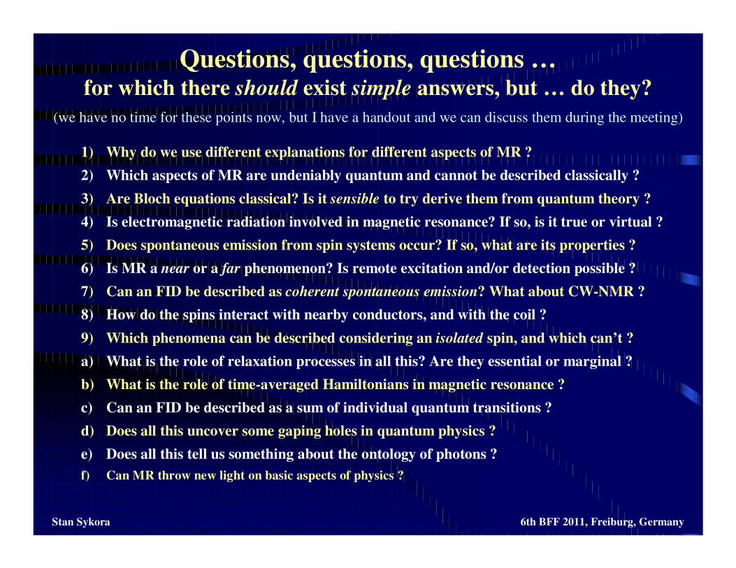
Questions, questions, questions …for which there should exist simple answers, but … do they?

1) Why do we use different explanations for different aspects of MR ?

2) Which aspects of MR are undeniably quantum and cannot be described classically ?

3) Are Bloch equations classical? Is it sensible to try derive them from quantum theory ?

4) Is electromagnetic radiation involved in magnetic resonance? If so, is it true or virtual ?

5) Does spontaneous emission from spin systems occur? If so, what are its properties ?

6) Is MR a near or a far phenomenon? Is remote excitation and/or detection possible ?

7) Can an FID be described as coherent spontaneous emission? What about CW-NMR ?

8) How do the spins interact with nearby conductors, and with the coil ?

9) Which phenomena can be described considering an isolated spin, and which can’t ?

a) What is the role of relaxation processes in all this? Are they essential or marginal ?

b) What is the role of time-averaged Hamiltonians in magnetic resonance ?

c) Can an FID be described as a sum of individual quantum transitions ?

d) Does all this uncover some gaping holes in quantum physics ?

e) Does all this tell us something about the ontology of photons ?

f) Can MR throw new light on basic aspects of physics ?

(we have no time for these points now, but I have a handout and we can discuss them during the meeting)


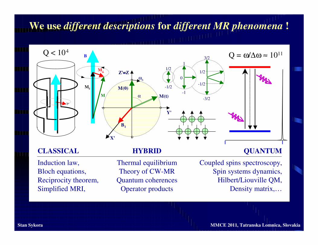
We use different descriptions for different MR phenomena !

CLASSICAL

Induction law,

Bloch equations,

Reciprocity theorem,

Simplified MRI,

QUANTUM

Coupled spins spectroscopy,

Spin systems dynamics,

Hilbert/Liouville QM,

Density matrix,…

HYBRID

Thermal equilibrium

Theory of CW-MR

Quantum coherences

Operator products

Q < 104Q = ω/∆ω ≈ 1011

Z'≡≡≡≡Z

Y'

X'

B1

M(0)

M(t)

ωn

α

-1/2

3/2

-3/2

1/2

0

1

-1

1/2

-1/2

B

M

M⊥⊥⊥⊥

M||

Stan Sykora MMCE 2011, Tatranska Lomnica, Slovakia

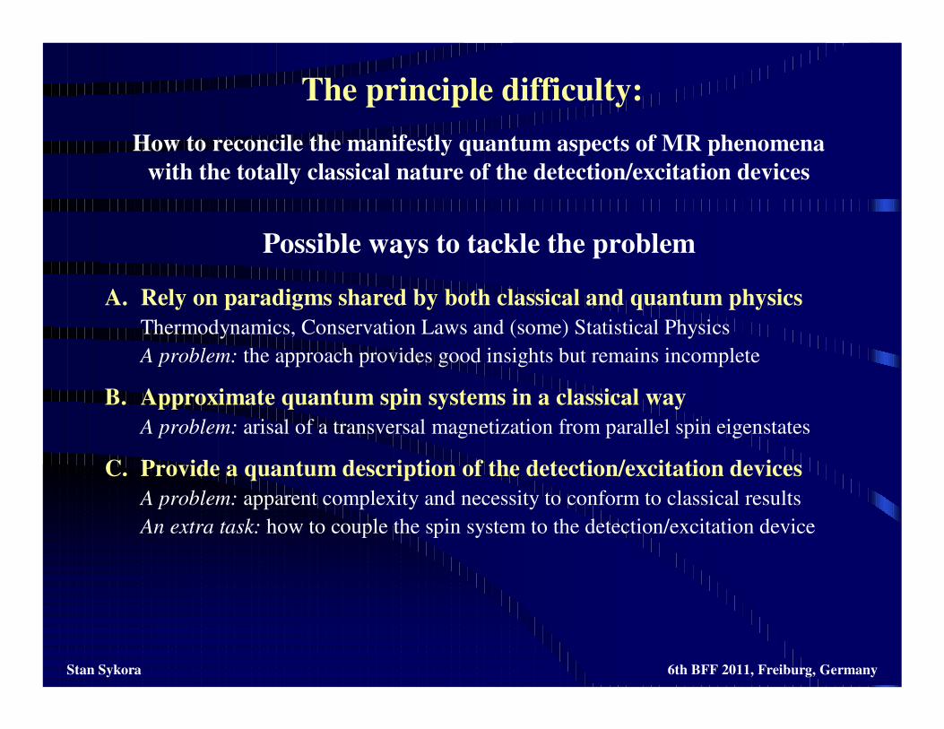
The principle difficulty:

How to reconcile the manifestly quantum aspects of MR phenomena

with the totally classical nature of the detection/excitation devices


Possible ways to tackle the problem

A. Rely on paradigms shared by both classical and quantum physics

Thermodynamics, Conservation Laws and (some) Statistical Physics

A problem: the approach provides good insights but remains incomplete

B. Approximate quantum spin systems in a classical way

A problem: arisal of a transversal magnetization from parallel spin eigenstates

C. Provide a quantum description of the detection/excitation devices

A problem: apparent complexity and necessity to conform to classical results

An extra task: how to couple the spin system to the detection/excitation device

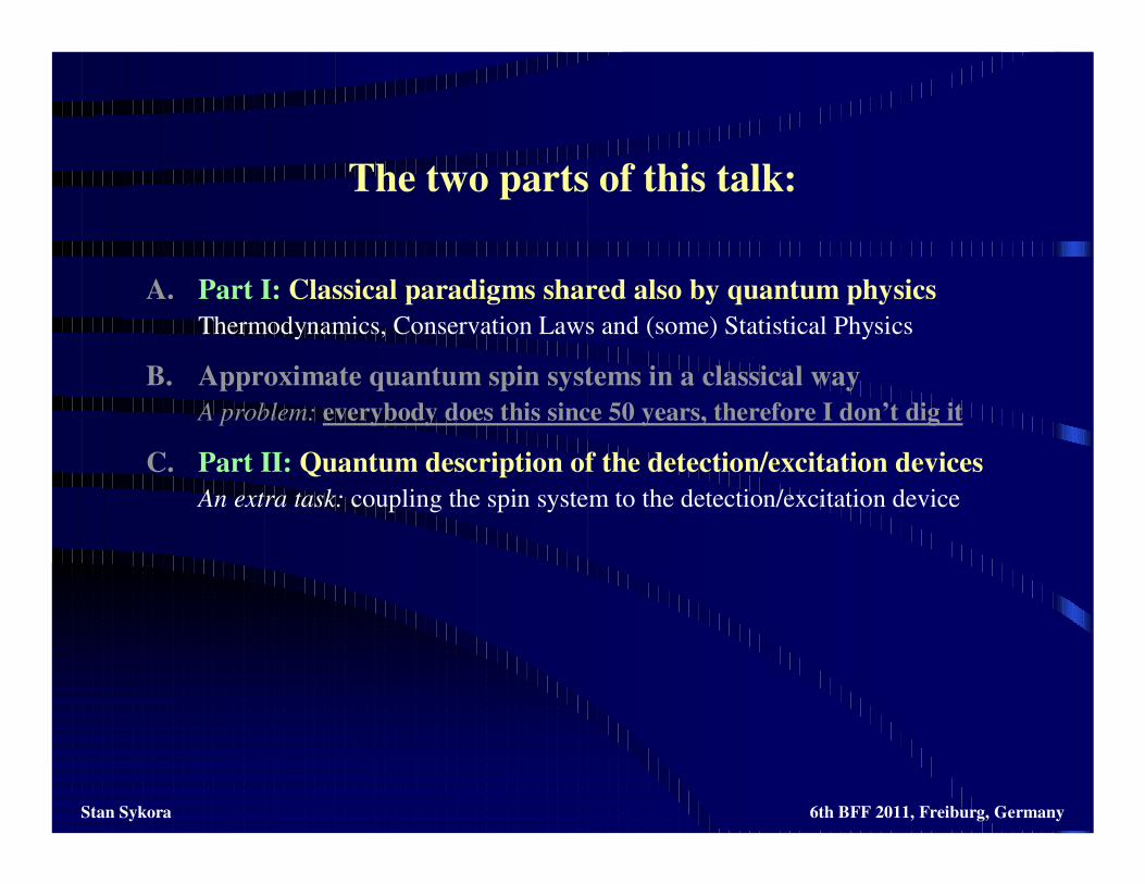
The two parts of this talk:


A. Part I: Classical paradigms shared also by quantum physics

Thermodynamics, Conservation Laws and (some) Statistical Physics

B. Approximate quantum spin systems in a classical way

A problem: everybody does this since 50 years, therefore I don’t dig it

C. Part II: Quantum description of the detection/excitation devices

An extra task: coupling the spin system to the detection/excitation device

Let us forget quantum physics for a while

and remember just the conservation of energy

(the first law of thermodynamics)


The physical system we will consider:

B = µH = µβJττττβ , where

µ is the permaebility, β a constant, and ττττβ a unit vector.

β and ττττβ depend only on the system’s geometry.

m = mττττm , where ττττmis a unit vector along m

L Loop and its Inductance

R Resistance (may be distributed)

J Electric current

P just a Point

B Magnetic Field

m Magnetic Dipole

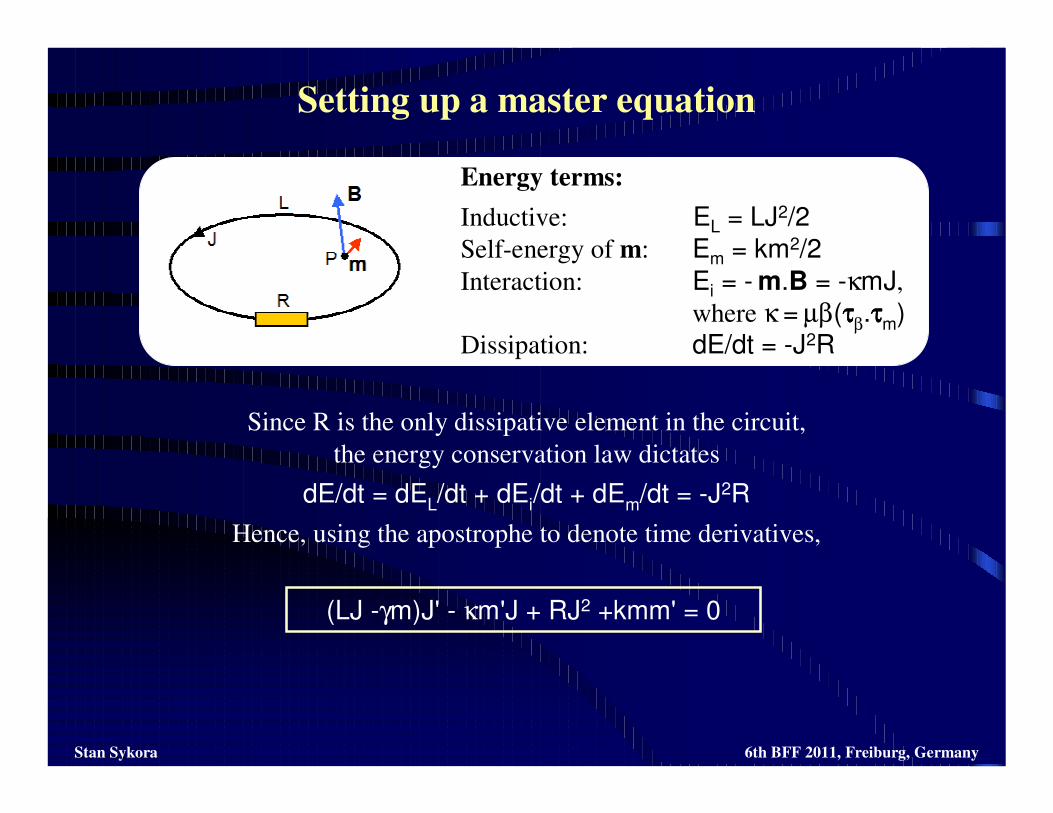
Setting up a master equation


Since R is the only dissipative element in the circuit,

the energy conservation law dictates

dE/dt = dEL/dt + dEi/dt + dEm/dt = -J2R

Hence, using the apostrophe to denote time derivatives,

(LJ -γm)J' - κm'J + RJ2 +kmm' = 0

Energy terms:

Inductive: EL = LJ2/2

Self-energy of m: Em = km2/2

Interaction: Ei = - m.B = -κmJ,

where κ = µβ(ττττβ.ττττm)Dissipation: dE/dt = -J2R

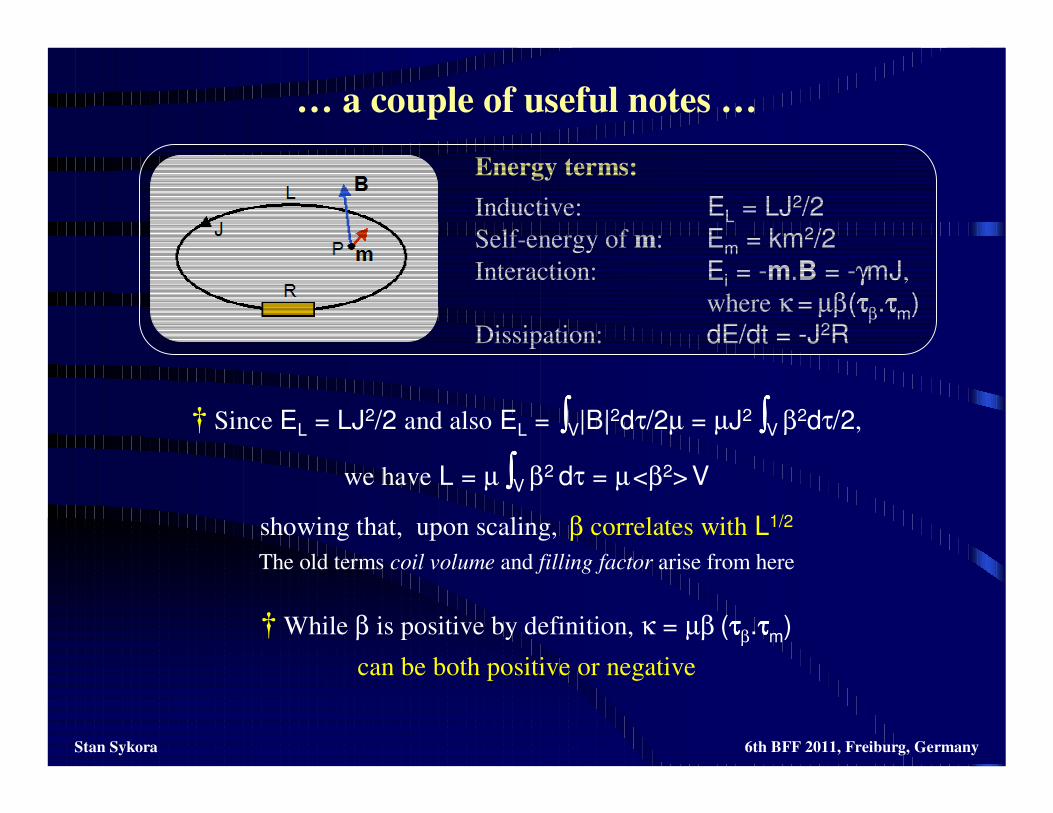
… a couple of useful notes …

Energy terms:

Inductive: EL = LJ2/2

Self-energy of m: Em = km2/2

Interaction: Ei = -m.B = -γmJ,

where κ = µβ(ττττβ.ττττm)Dissipation: dE/dt = -J2R


† Since EL = LJ2/2 and also EL = ∫∫∫∫V|B|2dτ/2µ = µJ2 ∫∫∫∫V β2dτ/2,

we have L = µ ∫∫∫∫V β2 dτ = µ<β2>V

showing that, upon scaling, β correlates with L1/2

The old terms coil volume and filling factor arise from here

† While β is positive by definition, κ = µβ (ττττβ.ττττm)

can be both positive or negative

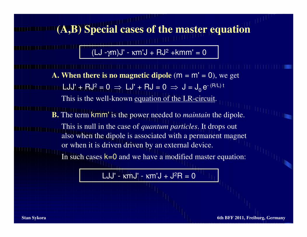
(A,B) Special cases of the master equation


A. When there is no magnetic dipole (m = m' = 0), we get

LJJ' + RJ2 = 0 ⇒ LJ' + RJ = 0 ⇒ J = J0 e- (R/L) t

This is the well-known equation of the LR-circuit.

B. The term kmm' is the power needed to maintain the dipole.

This is null in the case of quantum particles. It drops out

also when the dipole is associated with a permanent magnet

or when it is driven driven by an external device.

In such cases k=0 and we have a modified master equation:

(LJ -γm)J' - κm'J + RJ2 +kmm' = 0

LJJ' - κmJ' - κm'J + J2R = 0

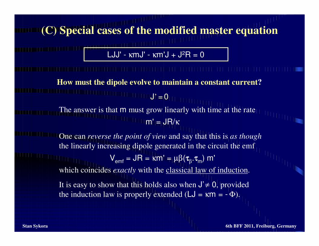
(C) Special cases of the modified master equation


LJJ' - κmJ' - κm'J + J2R = 0

How must the dipole evolve to maintain a constant current?

J’ =0

The answer is that m must grow linearly with time at the rate

m' = JR/κ

One can reverse the point of view and say that this is as though

the linearly increasing dipole generated in the circuit the emf

Vemf = JR = κm' = µβ(ττττβ.ττττm) m'

which coincides exactly with the classical law of induction.

It is easy to show that this holds also when J’≠ 0, provided

the induction law is properly extended (LJ = κm = - Φ).

(D-E) Oscillating magnetic dipoles


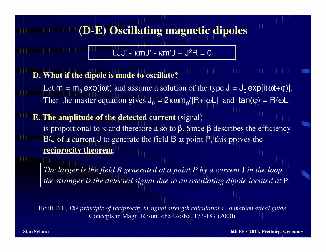
D. What if the dipole is made to oscillate?

Let m = m0 exp(iωt) and assume a solution of the type J = J0 exp[i(ωt+ϕ)].

Then the master equation gives J0 = 2κωm0/|R+iωL| and tan(ϕ) = R/ωL.

E. The amplitude of the detected current (signal)

is proportional to κ and therefore also to β. Since β describes the efficiency

B/J of a current J to generate the field B at point P, this proves the

reciprocity theorem:

LJJ' - κmJ' - κm'J + J2R = 0

The larger is the field B generated at a point P by a current J in the loop,

the stronger is the detected signal due to an oscillating dipole located at P.

Hoult D.I., The principle of reciprocity in signal strength calculations - a mathematical guide,

Concepts in Magn. Reson. <b>12</b>, 173-187 (2000).

(F) Current detection of oscillating dipoles


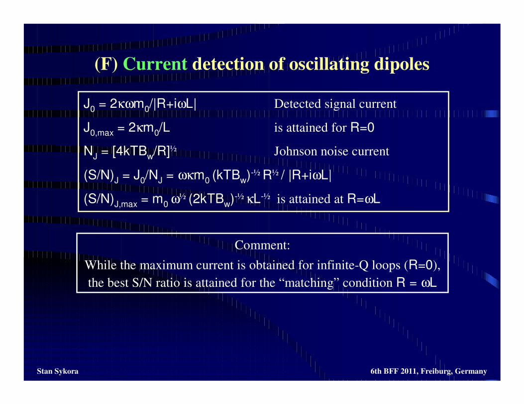
Comment:

While the maximum current is obtained for infinite-Q loops (R=0),

the best S/N ratio is attained for the “matching” condition R = ωL

J0 = 2κωm0/|R+iωL| Detected signal current

J0,max = 2κm0/L is attained for R=0

NJ = [4kTBw/R]½ Johnson noise current

(S/N)J = J0/NJ = ωκm0 (kTBw)-½ R½ / |R+iωL|

(S/N)J,max = m0 ω½ (2kTBw)-½ κL-½ is attained at R=ωL

(G) Voltage detection of oscillating dipoles


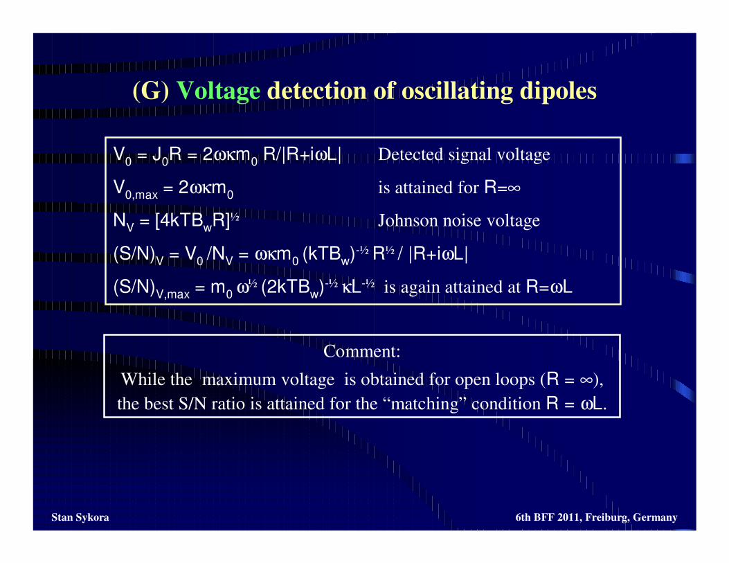
Comment:

While the maximum voltage is obtained for open loops (R = ∞),

the best S/N ratio is attained for the “matching” condition R = ωL.

V0 = J0R = 2ωκm0 R/|R+iωL| Detected signal voltage

V0,max = 2ωκm0 is attained for R=∞

NV = [4kTBwR]½ Johnson noise voltage

(S/N)V = V0 /NV = ωκm0 (kTBw)-½ R½ / |R+iωL|

(S/N)V,max = m0 ω½ (2kTBw)-½ κL-½ is again attained at R=ωL

(H) Power detection of oscillating dipoles


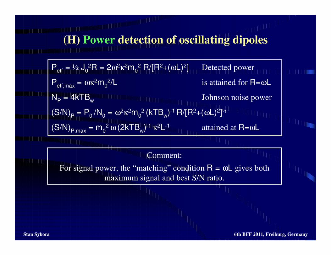
Comment:

For signal power, the “matching” condition R = ωL gives both

maximum signal and best S/N ratio.

Peff = ½ J02R = 2ω2κ2m0

2 R/[R2+(ωL)2] Detected power

Peff,max = ωκ2m02/L is attained for R=ωL

NP = 4kTBw Johnson noise power

(S/N)P = P0 /N0 = ω2κ2m02 (kTBw)-1 R/[R2+(ωL)2]½

(S/N)P,max = m02 ω (2kTBw)-1 κ2L-1 attained at R=ωL

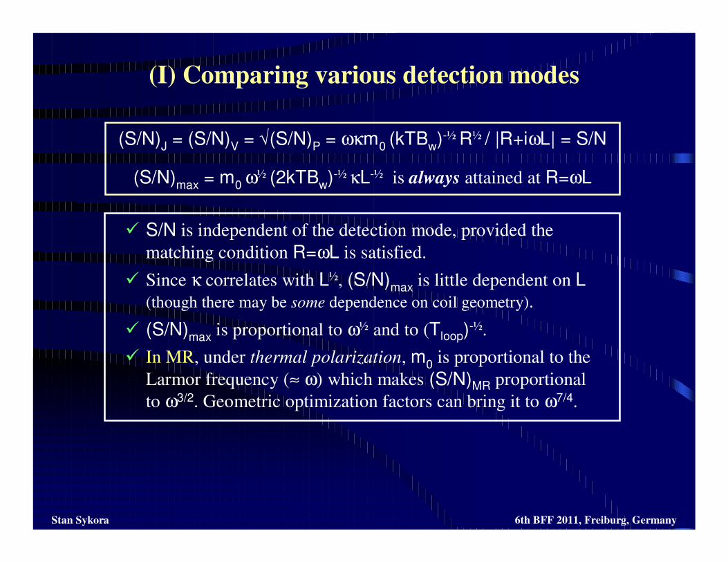
(I) Comparing various detection modes


S/N is independent of the detection mode, provided the

matching condition R=ωL is satisfied.

Since κ correlates with L½, (S/N)max is little dependent on L(though there may be some dependence on coil geometry).

(S/N)max is proportional to ω½ and to (Tloop)-½.

In MR, under thermal polarization, m0 is proportional to the

Larmor frequency (≈ ω) which makes (S/N)MR proportional

to ω3/2. Geometric optimization factors can bring it to ω7/4.

(S/N)J = (S/N)V = √(S/N)P = ωκm0 (kTBw)-½ R½ / |R+iωL| = S/N

(S/N)max = m0 ω½ (2kTBw)-½ κL-½ is always attained at R=ωL

Summing up what we did in Part I


Defined all energy terms

⇓⇓⇓⇓Applied thermodynamic laws such as

energy conservation and thermal noise formulae

⇓⇓⇓⇓and we have promptly obtained:

Circuit equations

Induction laws

Reciprocity theorem

Best signal detection conditions

Expressions for S/N ratios

Useful S/N rules

… etc

Note: making the circuit more complicated (LC) is useful and may uncover some

interesting engineering features, but nothing qualitatively new for the physicist

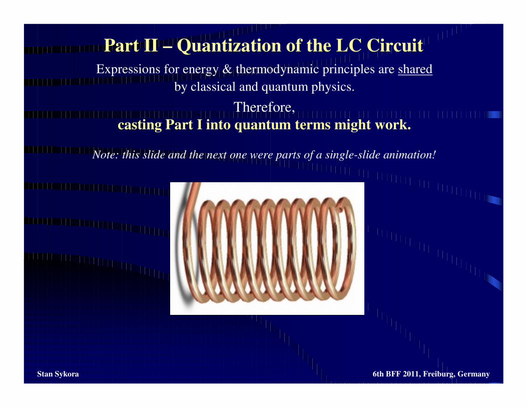
Part II – Quantization of the LC Circuit


Expressions for energy & thermodynamic principles are shared

by classical and quantum physics.

Therefore,

casting Part I into quantum terms might work.

Note: this slide and the next one were parts of a single-slide animation!

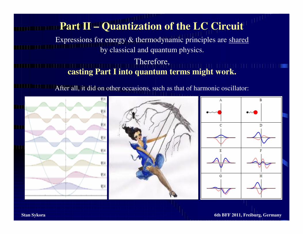
Part II – Quantization of the LC Circuit


Expressions for energy & thermodynamic principles are shared

by classical and quantum physics.

Therefore,

casting Part I into quantum terms might work.

After all, it did on other occasions, such as that of harmonic oscillator:

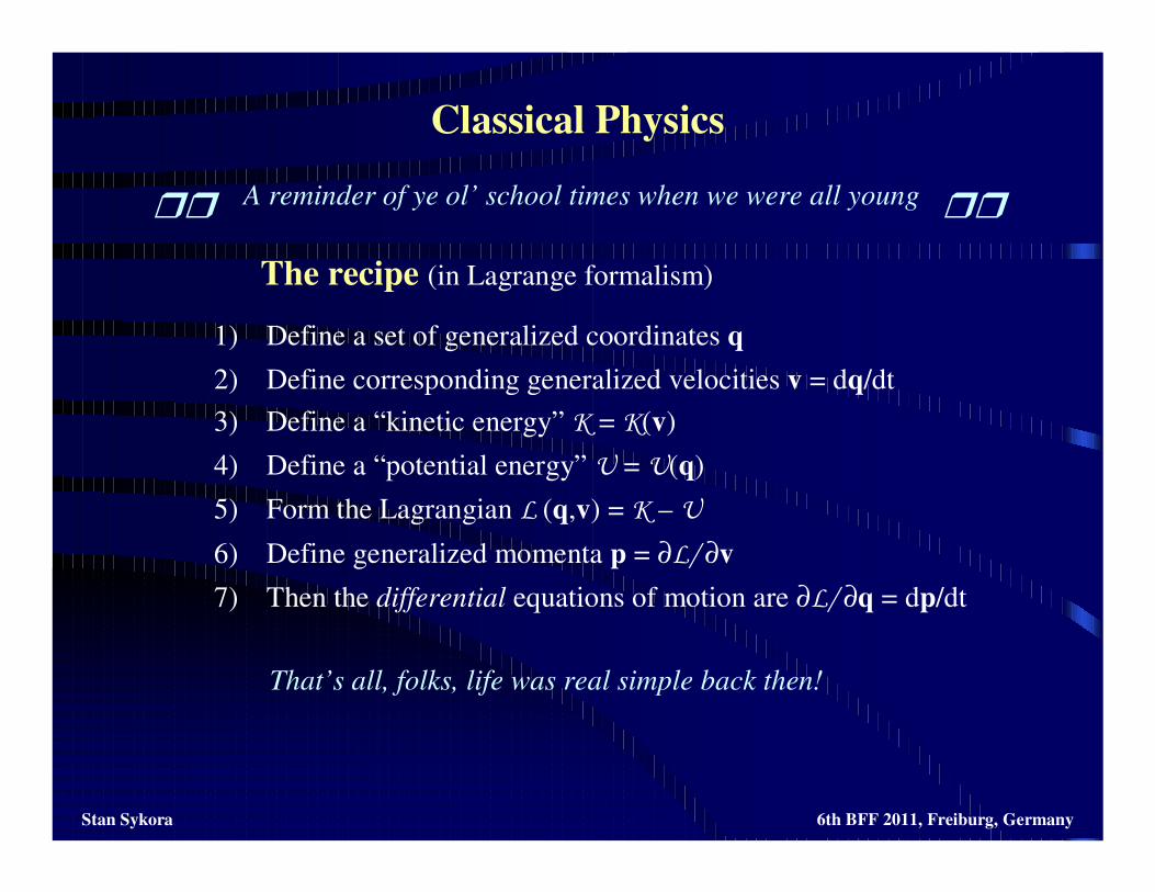
Classical Physics


A reminder of ye ol’ school times when we were all young

The recipe (in Lagrange formalism)

1) Define a set of generalized coordinates q

2) Define corresponding generalized velocities v = dq/dt

3) Define a “kinetic energy” K = K(v)

4) Define a “potential energy” U = U(q)

5) Form the Lagrangian L (q,v) = K – U

6) Define generalized momenta p = ∂L/ ∂v

7) Then the differential equations of motion are ∂L/ ∂q = dp/dt

That’s all, folks, life was real simple back then!

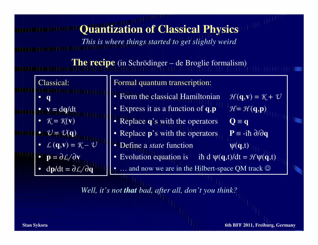
Quantization of Classical Physics


This is where things started to get slightly weird

The recipe (in Schrödinger – de Broglie formalism)

Well, it’s not that bad, after all, don’t you think?

Classical:

• q

• v = dq/dt

• K = K(v)

• U = U(q)

• L (q,v) = K – U

• p = ∂L/ ∂v

• dp/dt = ∂L/ ∂q

Formal quantum transcription:

• Form the classical Hamiltonian H (q,v) = K + U

• Express it as a function of q,p H = H (q,p)

• Replace q’s with the operators Q ≡ q

• Replace p’s with the operators P ≡ -iħ ∂/∂q

• Define a state function ψ(q,t)

• Evolution equation is iħ d ψ(q,t)/dt = H ψ(q,t)

• … and now we are in the Hilbert-space QM track

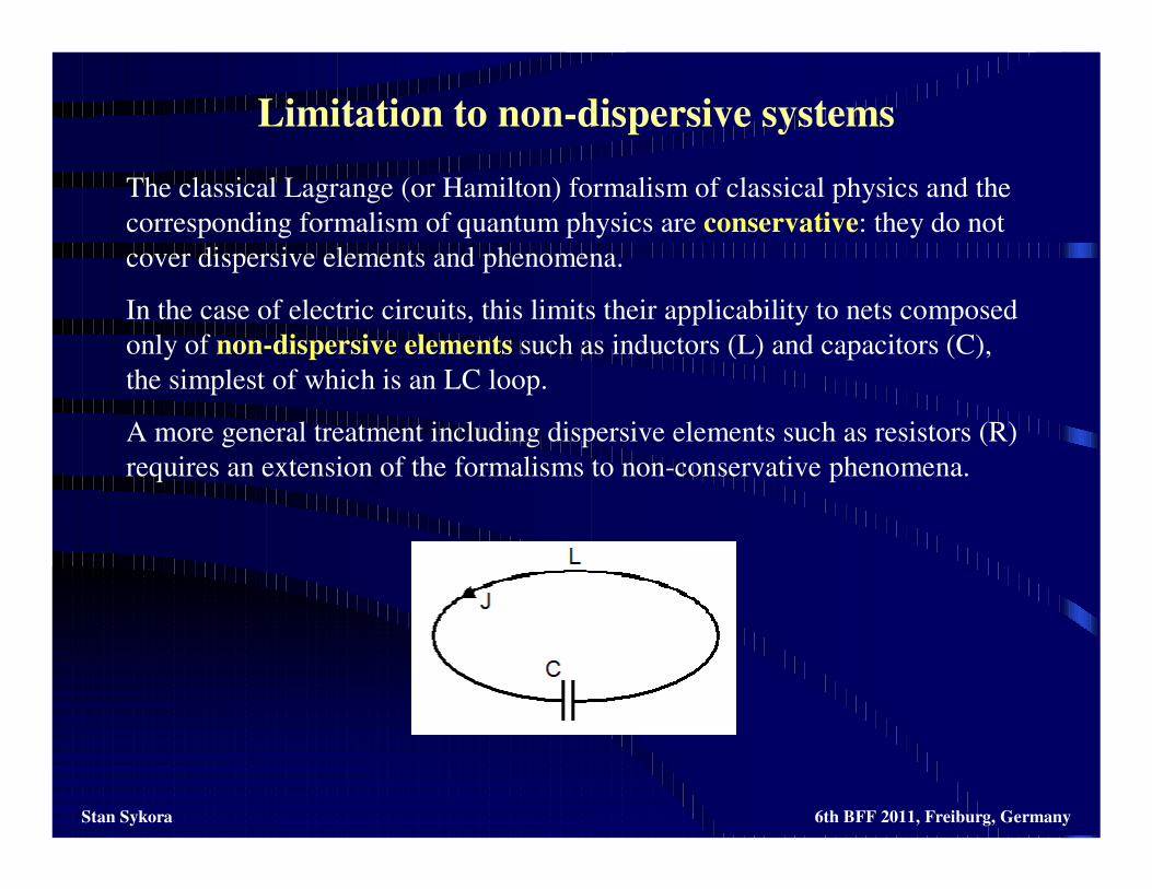
Limitation to non-dispersive systems


The classical Lagrange (or Hamilton) formalism of classical physics and the

corresponding formalism of quantum physics are conservative: they do not

cover dispersive elements and phenomena.

In the case of electric circuits, this limits their applicability to nets composed

only of non-dispersive elements such as inductors (L) and capacitors (C),

the simplest of which is an LC loop.

A more general treatment including dispersive elements such as resistors (R)

requires an extension of the formalisms to non-conservative phenomena.

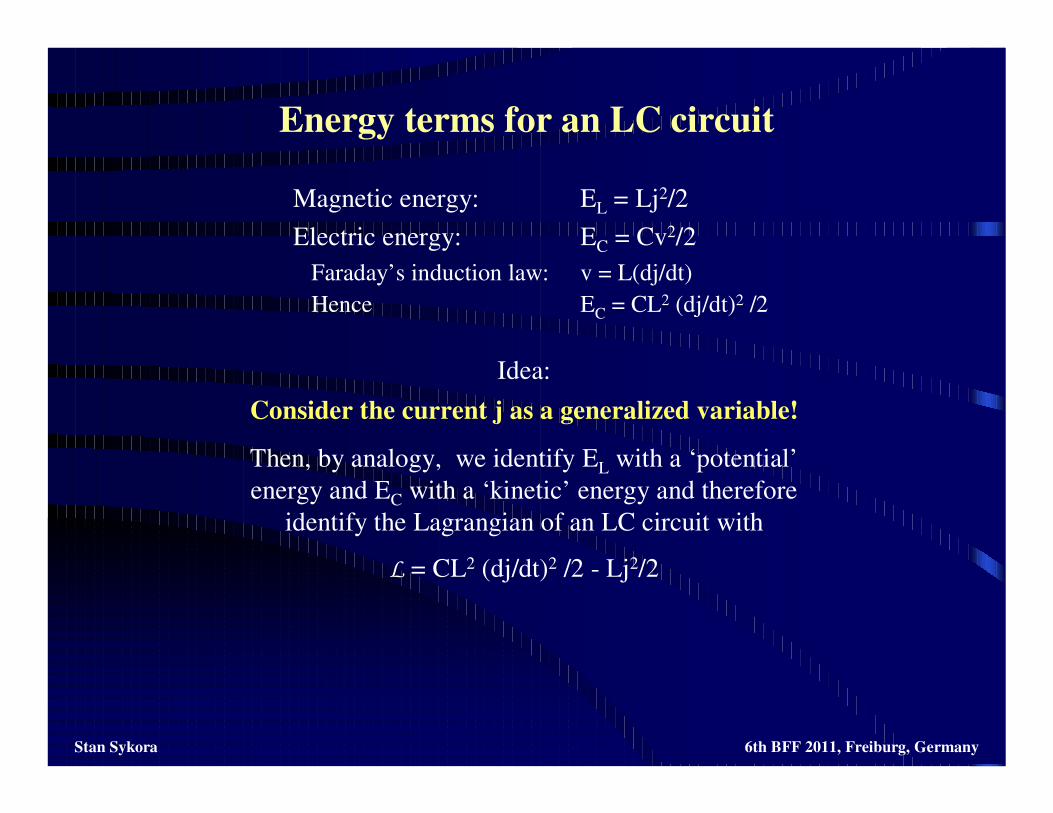
Energy terms for an LC circuit


Magnetic energy: EL = Lj2/2

Electric energy: EC = Cv2/2

Faraday’s induction law: v = L(dj/dt)

Hence EC = CL2 (dj/dt)2 /2

Idea:

Consider the current j as a generalized variable!

Then, by analogy, we identify EL with a ‘potential’

energy and EC with a ‘kinetic’ energy and therefore

identify the Lagrangian of an LC circuit with

L = CL2 (dj/dt)2 /2 - Lj2/2

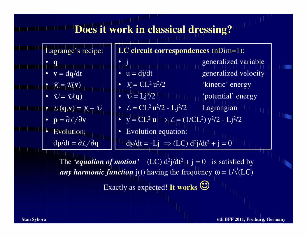
Does it work in classical dressing?


Lagrange’s recipe:

• q

• v = dq/dt

• K = K(v)

• U = U(q)

• L (q,v) = K – U

• p = ∂L/ ∂v

• Evolution:

dp/dt = ∂L/ ∂q

LC circuit correspondences (nDim=1):

• j generalized variable

• u = dj/dt generalized velocity

• K = CL2 u2/2 ‘kinetic’ energy

• U = Lj2/2 ‘potential’ energy

• L = CL2 u2/2 - Lj2/2 Lagrangian

• y = CL2 u ⇒ L = (1/CL2) y2/2 - Lj2/2

• Evolution equation:

dy/dt = -Lj ⇒ (LC) d2j/dt2 + j = 0

The ‘equation of motion’ (LC) d2j/dt2 + j = 0 is satisfied by

any harmonic function j(t) having the frequency ω = 1/√(LC)

Exactly as expected! It works

LC circuit in quantum dressing


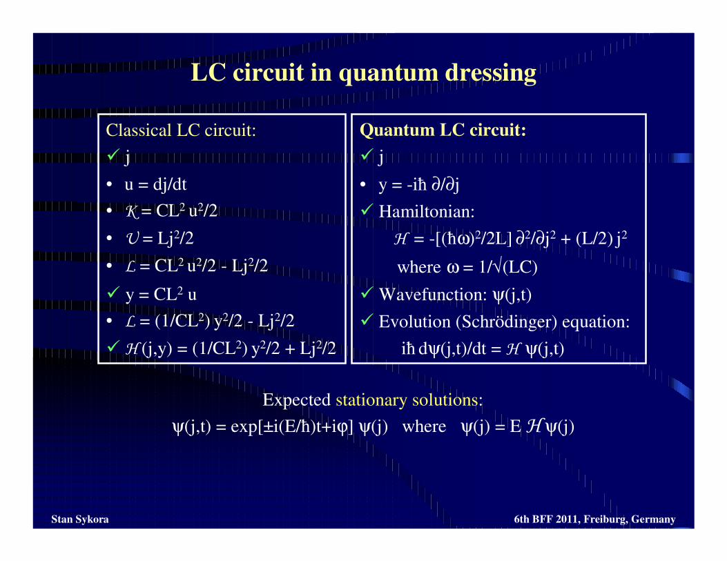
Classical LC circuit:

j

• u = dj/dt

• K = CL2 u2/2

• U = Lj2/2

• L = CL2 u2/2 - Lj2/2

y = CL2 u

• L = (1/CL2) y2/2 - Lj2/2

H (j,y) = (1/CL2) y2/2 + Lj2/2

Quantum LC circuit:

j

• y = -iħ ∂/∂j

Hamiltonian:

H = -[(ħω)2/2L] ∂2/∂j2 + (L/2) j2

where ω = 1/√(LC)

Wavefunction: ψ(j,t)

Evolution (Schrödinger) equation:

iħ dψ(j,t)/dt = H ψ(j,t)

Expected stationary solutions:

ψ(j,t) = exp[±i(E/ħ)t+iϕ] ψ(j) where ψ(j) = E H ψ(j)

Quantum LC Circuit and the Harmonic Oscillator


Quantum LC with frequency ω:

• j

• Hamiltonian:

H = -[(ħω)2/2L] ∂2/∂j2 + (L/2) j2

• Wavefunction: ψ(j,t)

• Schrödinger equation:

iħ dψ(j,t)/dt = H ψ(j,t)

Quantum HO with frequency ω:

• x

• Hamiltonian:

H = -[ħ2/2m] ∂2/∂x2 + (mω2/2) x2

• Wavefunction: ψ(x,t)

• Schrödinger equation:

iħ dψ(x,t)/dt = H ψ(x,t)

A perfect correspondence can be achieved by setting

m ≈ CL2 = L/ω2

saving a lot of work in finding the stationary solutions

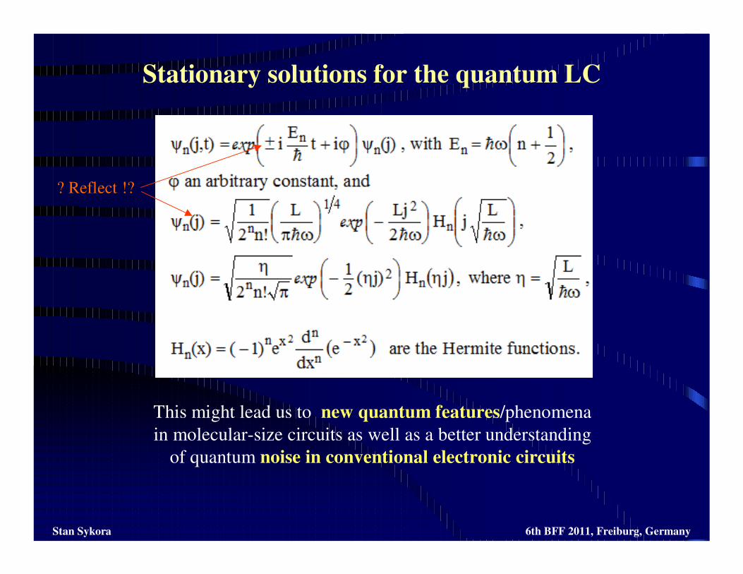
Stationary solutions for the quantum LC


This might lead us to new quantum features/phenomena

in molecular-size circuits as well as a better understanding

of quantum noise in conventional electronic circuits

? Reflect !?

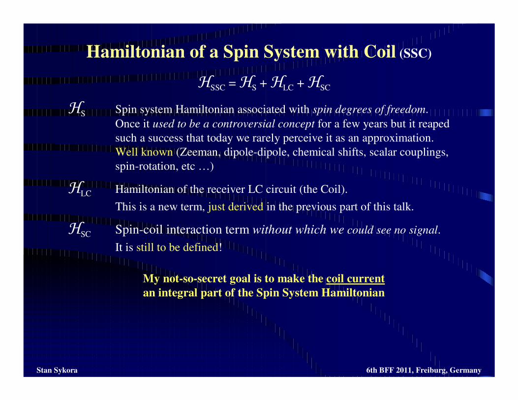
Hamiltonian of a Spin System with Coil (SSC)


My not-so-secret goal is to make the coil current

an integral part of the Spin System Hamiltonian

HSSC = HS + HLC + HSC

HS Spin system Hamiltonian associated with spin degrees of freedom.

Once it used to be a controversial concept for a few years but it reaped

such a success that today we rarely perceive it as an approximation.

Well known (Zeeman, dipole-dipole, chemical shifts, scalar couplings,

spin-rotation, etc …)

HLC Hamiltonian of the receiver LC circuit (the Coil).

This is a new term, just derived in the previous part of this talk.

HSC Spin-coil interaction term without which we could see no signal.

It is still to be defined!

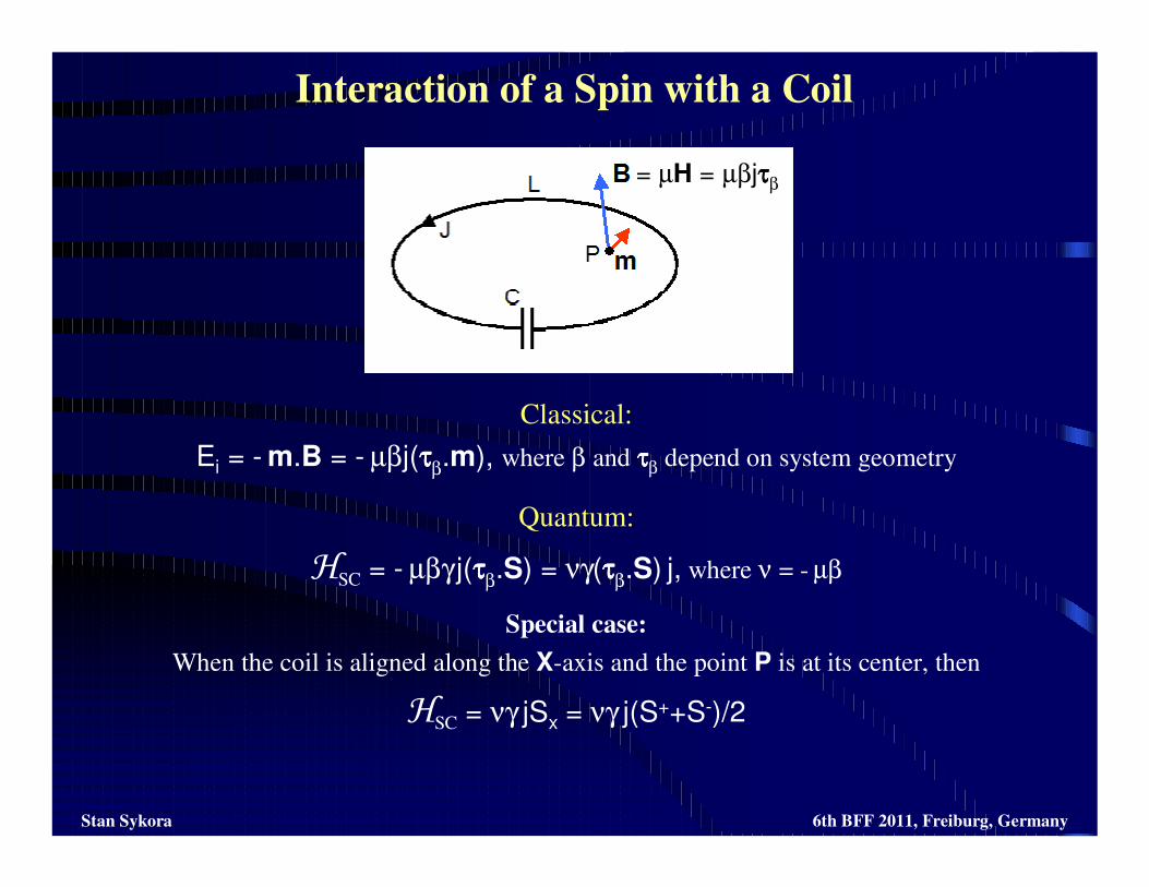
Interaction of a Spin with a Coil


Classical:

Ei = - m.B = - µβj(ττττβ.m), where β and ττττβ depend on system geometry

Quantum:

HSC = - µβγ j(ττττβ.S) = νγ(ττττβ.S) j, where ν = - µβ

Special case:

When the coil is aligned along the X-axis and the point P is at its center, then

HSC = νγ jSx = νγ j(S++S-)/2

= µH = µβjττττβ

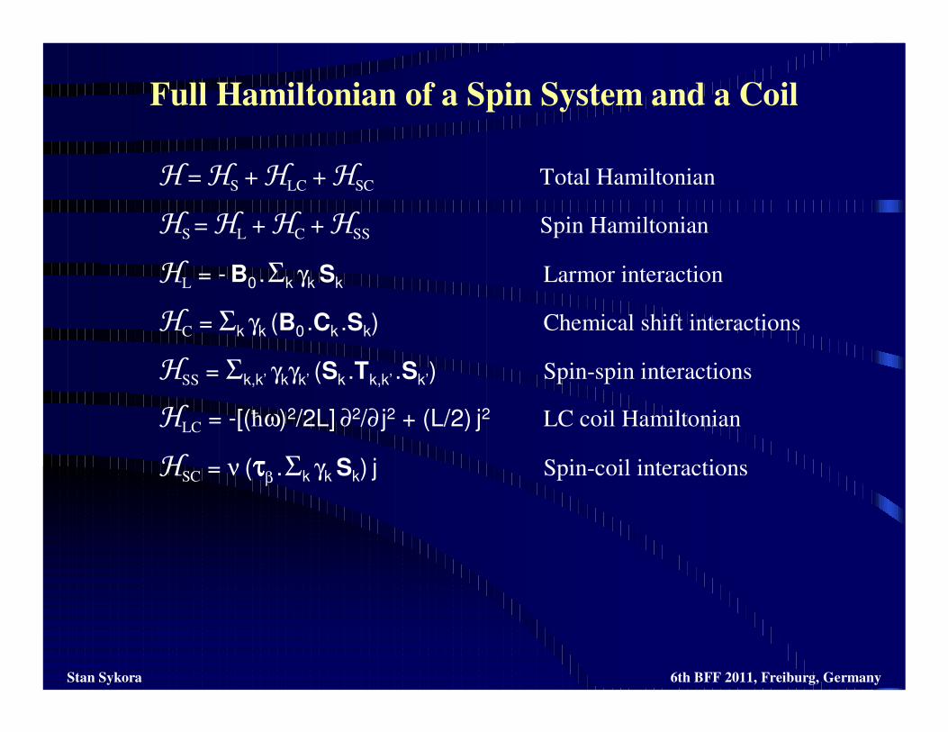
Full Hamiltonian of a Spin System and a Coil


H = HS + HLC + HSC Total Hamiltonian

HS = HL + HC + HSS Spin Hamiltonian

HL = - B0 .Σk γk Sk Larmor interaction

HC = Σk γk (B0 .Ck .Sk) Chemical shift interactions

HSS = Σk,k’ γkγk’ (Sk .Tk,k’ .Sk’) Spin-spin interactions

HLC = -[(ħω)2/2L] ∂2/∂ j2 + (L/2) j2 LC coil Hamiltonian

HSC = ν (ττττβ .Σk γk Sk) j Spin-coil interactions

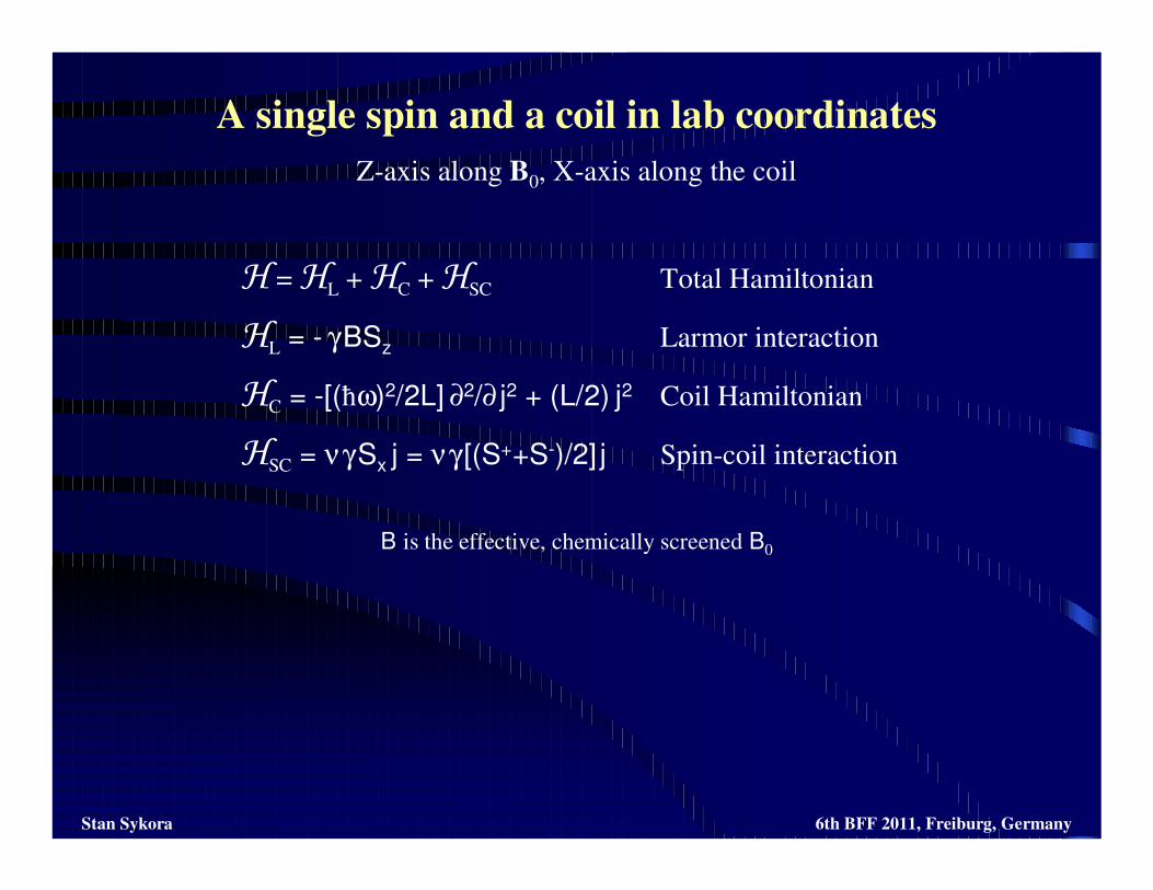
A single spin and a coil in lab coordinates


H = HL + HC + HSC Total Hamiltonian

HL = - γBSz Larmor interaction

HC = -[(ħω)2/2L] ∂2/∂ j2 + (L/2) j2 Coil Hamiltonian

HSC = νγSx j = νγ [(S++S-)/2] j Spin-coil interaction

Z-axis along B0, X-axis along the coil

B is the effective, chemically screened B0

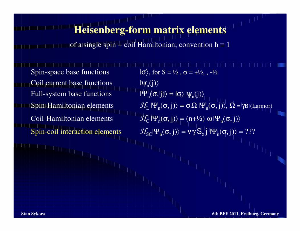
Heisenberg-form matrix elements


Spin-space base functions |σ⟩, for S = ½ , σ = +½, , -½

Coil current base functions |ψn(j)⟩

Full-system base functions |Ψn(σ, j)⟩ = |σ⟩ |ψn(j)⟩

Spin-Hamiltonian elements HL |Ψn(σ, j)⟩ = σΩ |Ψn(σ, j)⟩, Ω = γB (Larmor)

Coil-Hamiltonian elements HC |Ψn(σ, j)⟩ = (n+½) ω |Ψn(σ, j)⟩

Spin-coil interaction elements HSC|Ψn(σ, j)⟩ = νγ Sx j |Ψn(σ, j)⟩ = ???

of a single spin + coil Hamiltonian; convention ħ ≡ 1

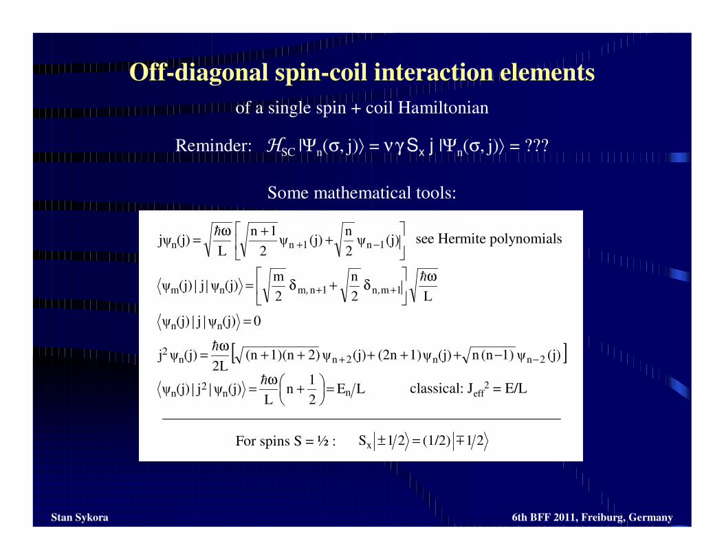
Off-diagonal spin-coil interaction elements


Reminder: HSC |Ψn(σ, j)⟩ = νγ Sx j |Ψn(σ, j)⟩ = ???

of a single spin + coil Hamiltonian

Some mathematical tools:

+

+ω= −+ (j)ψ

2

n(j)ψ

2

1n

L(j)jψ 1n1nn

h

0(j)ψj(j)ψ nn =||

LE2

1n

L(j)ψj(j)ψ nn

2n =

+

ω=h

||

L2

n

2

m (j)ψj(j)ψ 1mn1nmnm

ω

δ+δ= ++

h

,,||

[ ](j)ψ1)(nn(j)ψ1)(2n(j)ψ2)1)(n(n2L

(j)ψj 2nn2nn2

−+ −+++++ω

=h

see Hermite polynomials

classical: Jeff2 = E/L

21 (1/2)21S x m=±For spins S = ½ :

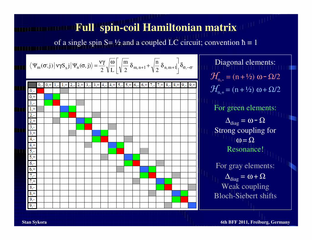
Full spin-coil Hamiltonian matrix


of a single spin S= ½ and a coupled LC circuit; convention ħ ≡ 1

Diagonal elements:

Hn,- = (n + ½) ω- Ω/2

Hn,+ = (n + ½) ω+ Ω/2

For green elements:

∆diag = ω- ΩStrong coupling for

ω = ΩResonance!

For gray elements:

∆diag = ω + ΩWeak coupling

Bloch-Siebert shifts

',,,,,' σ−σ++ δ

δ+δ

ωνγ=σΨνγσΨ 1mn1nmnxm

2

n

2

m

L2 )j( jS )j(

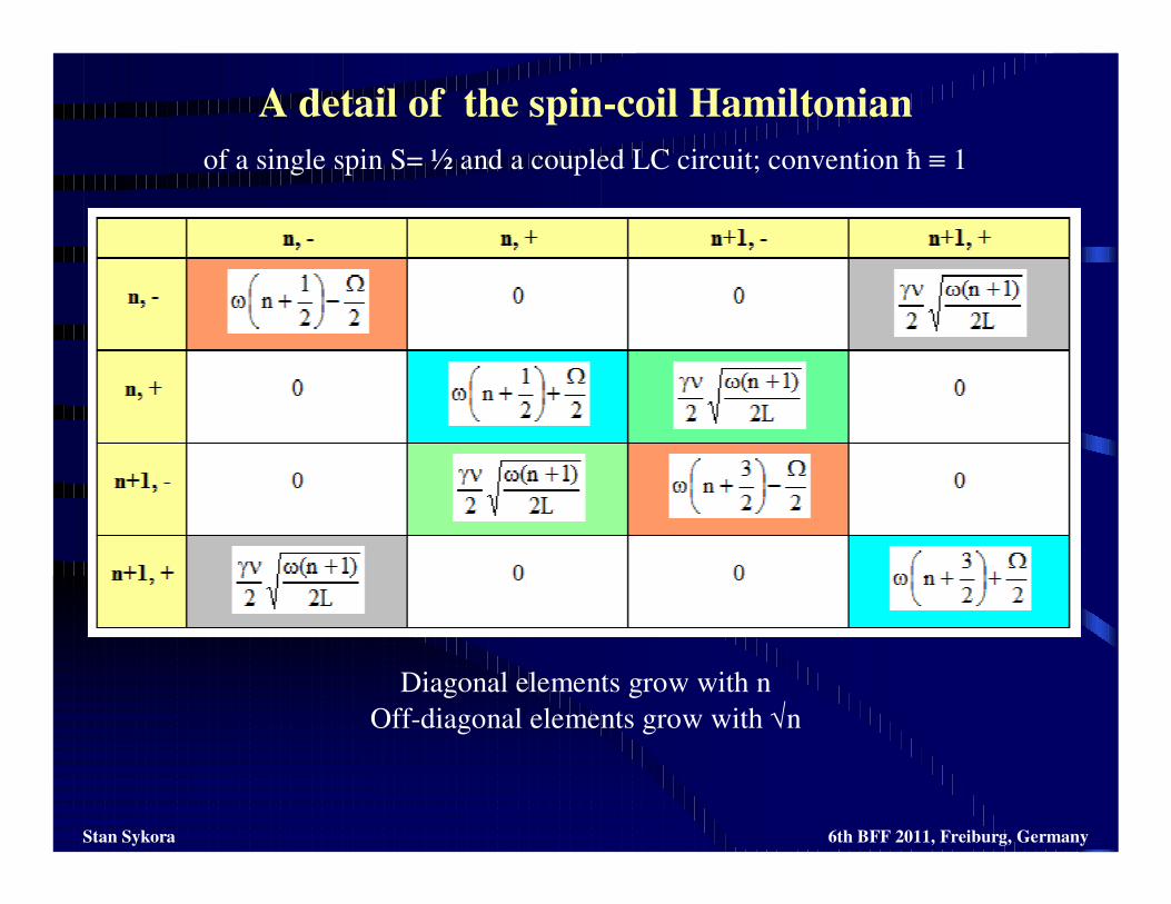
A detail of the spin-coil Hamiltonian


of a single spin S= ½ and a coupled LC circuit; convention ħ ≡ 1

Diagonal elements grow with n

Off-diagonal elements grow with √n

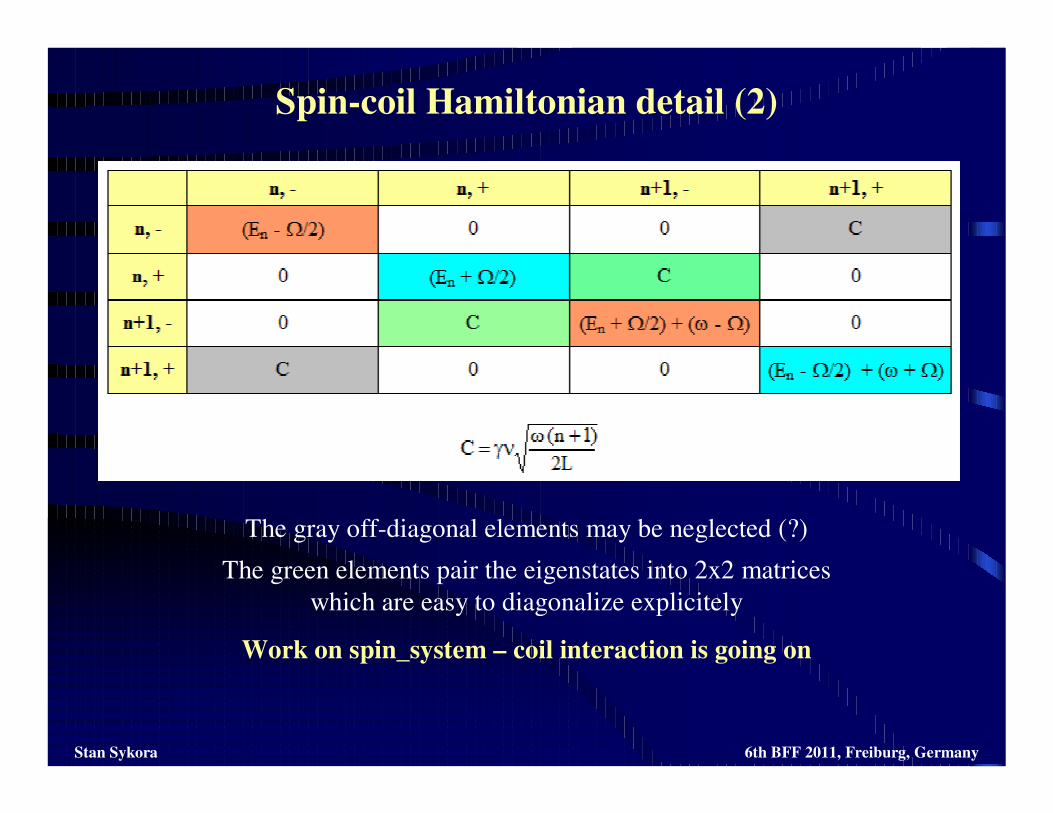
Spin-coil Hamiltonian detail (2)


The gray off-diagonal elements may be neglected (?)

The green elements pair the eigenstates into 2x2 matrices

which are easy to diagonalize explicitely

Work on spin_system – coil interaction is going on

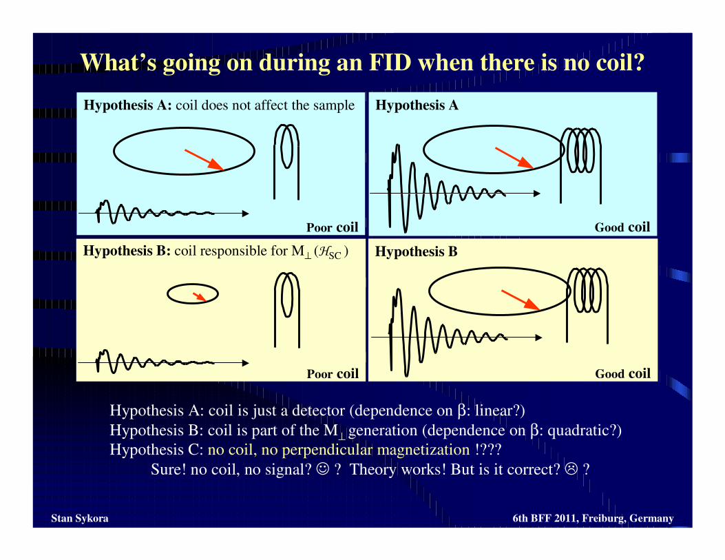
What’s going on during an FID when there is no coil?


Hypothesis B

Good coil

Hypothesis B: coil responsible for M⊥ (HSC )

Poor coil

Hypothesis A: coil does not affect the sample

Poor coil

Hypothesis A

Good coil

Hypothesis A: coil is just a detector (dependence on β: linear?)

Hypothesis B: coil is part of the M⊥ generation (dependence on β: quadratic?)

Hypothesis C: no coil, no perpendicular magnetization !???

Sure! no coil, no signal? ? Theory works! But is it correct? ?

Limb lost, Wisdom gained


Thank you – and let’s discuss!

Erwin, a would be friend,

closed me in his Box; yet,

despite all odds, out I got

- and all on my own -

loosing just a limb in the

nasty quantum foam!

Most amazing things I saw,

states mixed and uncertain

Erwin could never imagine!

For the Box was Closed!

Inaccessible to his scrutiny

while I, I stayed Within.

Documents

Some Thermodynamic and Quantum Aspects of … · Some Thermodynamic and Quantum Aspects of NMR Signal Detection Stanislav Sýkora ... Does all this uncover some gaping holes in quantum