Some Topics In Multivariate Regression

Some Topics

• We need to address some small topics that are often come up in multivariate regression.

• I will illustrate them using the Housing example.

Some Topics

1. Confidence intervals

2. Scale of data

3. Functional Form

4. Tests of multi-coefficient hypotheses

Woldridge refs to date

• Chapter 1• Chapter 2.1, 2.2,2.5• Chapter 3.1,3.2,3.3• Chapter 4.1, 4.2, 4.3, 4.4

Confidence Intervals (4.3)• We can construct an interval within which the

true value of the parameter lies• We have seen that

– P(-1.96 ≤ t ≤ 1.96)=0.95 for large N-K• More generally:

1))(*)(*(

1))(

(

1)(

OLScOLSOLScOLS

cOLS

OLSc

cc

bsetbbsetbP

tbse

btP

tttP

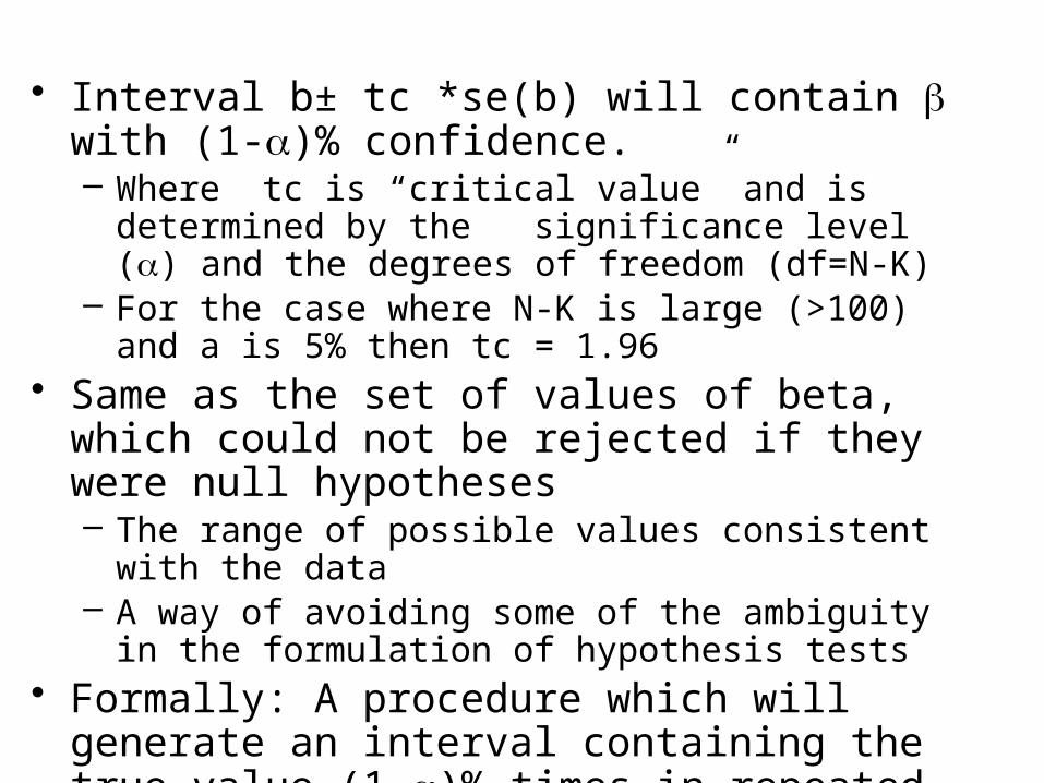
• Interval b± tc *se(b) will contain b with (1-a)% confidence.– Where tc is “critical value” and is determined by the

significance level (a) and the degrees of freedom (df=N-K)

– For the case where N-K is large (>100) and a is 5% then tc = 1.96

• Same as the set of values of beta, which could not be rejected if they were null hypotheses – The range of possible values consistent with the data – A way of avoiding some of the ambiguity in the

formulation of hypothesis tests• Formally: A procedure which will generate an

interval containing the true value (1-a)% times in repeated samples

Level Option

• Stata command: regress … , level(95)• Note: in assignments I want you to do it manually

regress price inc_pc hstock_pc if year<=1997

Source | SS df MS Number of obs = 28-------------+------------------------------ F( 2, 25) = 88.31 Model | 1.1008e+10 2 5.5042e+09 Prob > F = 0.0000 Residual | 1.5581e+09 25 62324995.9 R-squared = 0.8760-------------+------------------------------ Adj R-squared = 0.8661 Total | 1.2566e+10 27 465423464 Root MSE = 7894.6

------------------------------------------------------------------------------ price | Coef. Std. Err. t P>|t| [95% Conf. Interval]-------------+---------------------------------------------------------------- inc_pc | 10.39438 1.288239 8.07 0.000 7.741204 13.04756 hstock_pc | -637054.1 174578.5 -3.65 0.001 -996605.3 -277503 _cons | 135276.6 35433.83 3.82 0.001 62299.24 208253.9------------------------------------------------------------------------------

Scale (2.4 & 6.1)

• The scale of the data may matter– i.e. whether we measure house prices in € or

€bn or even £ or $• Exercise: try this with housing or

consumption examples• Basic model: yi = b1 + b2 xi + ui

• Change scale of xi : xi* = xi/c– Estimate: yi = b1

* + b2* xi*+ ui

• b2*= c.b2

• se(b2) = c.se(b2)

• Slope coefficient and se change, all other statistics (t-stats, R2, F, etc.) unchanged.

• Change scale of yi : yi* = yi/c – Estimate y*i = b1

* + b2* xi + ui

• b2*= b2 /c

• b1*= b1 /c

• se(b2) = se(b2)/c

• se(b1) = se(b1)/c

• t-stats, R2, F unchanged

• Both X and Y rescaled yi* = yi/c, xi* = xi/c– Estimate y*i = b1

* + b2* x* + ui

– If rescaled by same amount: – b1*= b1 /c se(b1) = se(b1)/c

– b2 and se(b2) unchanged

– t-stats, R2, F unchanged

Functional Form (6.2)

• Four common functional forms– Linear: qt = a + pt + ut

– Log-Log: lnqt = a + lnpt + ut

– Semilog: qt = a + lnpt + ut

or lnqt = a + pt + ut

• How to choose?– Which fits the data best (cannot compare R2 unless y is same)– Which is most convenient (do we want elasticity, rate of return?)– How trade-off two goals

Elasticity and Marginal Effects

pqp

qupq

qpp

qupq

p

q

p

qupq

q

p

p

qupq

q

p

p

q

p

q

ttt

ttt

ttt

ttt

lnln

lnln

ln

lnlnln

Two housing models

• The level variables: marginal effects

regress price inc_pc hstock_pc if year<=1997

Source | SS df MS Number of obs = 28-------------+------------------------------ F( 2, 25) = 88.31 Model | 1.1008e+10 2 5.5042e+09 Prob > F = 0.0000 Residual | 1.5581e+09 25 62324995.9 R-squared = 0.8760-------------+------------------------------ Adj R-squared = 0.8661 Total | 1.2566e+10 27 465423464 Root MSE = 7894.6

------------------------------------------------------------------------------ price | Coef. Std. Err. t P>|t| [95% Conf. Interval]-------------+---------------------------------------------------------------- inc_pc | 10.39438 1.288239 8.07 0.000 7.741204 13.04756 hstock_pc | -637054.1 174578.5 -3.65 0.001 -996605.3 -277503 _cons | 135276.6 35433.83 3.82 0.001 62299.24 208253.9------------------------------------------------------------------------------

• Log on log formulation

regress lprice linc lh if year<=1997

Source | SS df MS Number of obs = 28-------------+------------------------------ F( 2, 25) = 86.21 Model | .791044208 2 .395522104 Prob > F = 0.0000 Residual | .11469849 25 .00458794 R-squared = 0.8734-------------+------------------------------ Adj R-squared = 0.8632 Total | .905742698 27 .033546026 Root MSE = .06773

------------------------------------------------------------------------------ lprice | Coef. Std. Err. t P>|t| [95% Conf. Interval]-------------+---------------------------------------------------------------- linc | 1.67764 .2168253 7.74 0.000 1.23108 2.1242 lh | -2.011761 .5228058 -3.85 0.001 -3.0885 -.9350227 _cons | -7.039114 2.687196 -2.62 0.015 -12.5735 -1.504731------------------------------------------------------------------------------

F-tests

• Often we will want to test joint hypotheses– i.e. hypotheses that involve more than one

coefficient– Linear restrictions

• Three examples (using the log model)1. H0: bH = 0 & bI= 0 H1: bH ≠ 0 or bI ≠0

2. H0: bH = 0 & bI= 1 H1: bH ≠ 0 or bI ≠1

3. H0: bH + bI= 1 H1: bH + bI ≠ 1

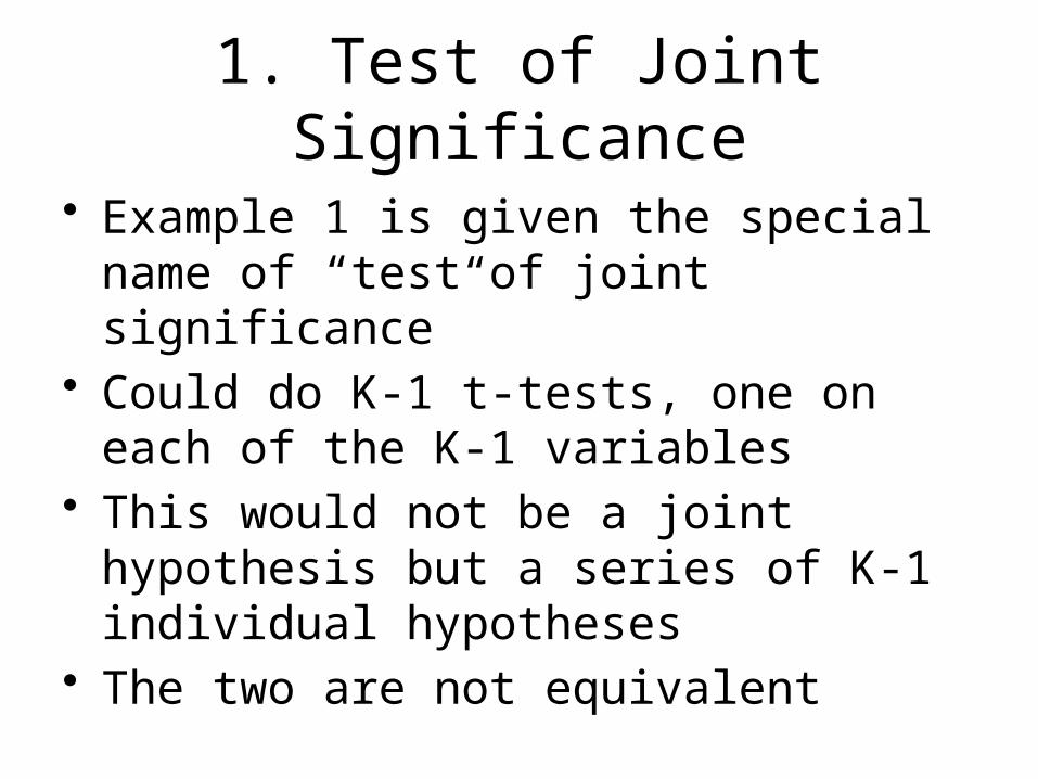
1. Test of Joint Significance

• Example 1 is given the special name of “test of joint significance”

• Could do K-1 t-tests, one on each of the K-1 variables

• This would not be a joint hypothesis but a series of K-1 individual hypotheses

• The two are not equivalent

Why Joint Hypotheses matter

• Recall the sampling makes the estimators random variables

• Estimators of different coefficients are correlated random variables

• All the coeff are estimated from same sample in any one regression

• Making statements about one coefficient implies a statement about another

• Formally P(b2=0).P(b3 =0) P(b2=b3 =0)

• So the set of regressions in which both are zero is smaller than the set in which either one are zero

• This intuition holds for more general hypotheses.

Testing Joint Significance

• As we look at all the variables it is natural to focus on the ESS

• We form a test statistic

• If the null hypothesis is true the ESS will be zero and RSS will be large

• So we can reject the null hypothesis if the test statistic is greater than zero

• How much greater?• Greater than a critical value got from the

F-distribution tables with three parameters– Significance level– Df1=K-1– Df2=N-K

• The test is so useful it is reported by stata

Formal Procedure

1. State the Hypothesis we want to testH0: bH = 0 & bI= 0 H1: bH ≠ 0 or bI ≠0

2. Calculate the test statistic assuming that null is true. 86.21

3. Critical Value: – F(2,25)= 3.39 at 5% significance level– Stata: di invFtail(2,25,0.05)

4. As F>critical value we can reject the null hypothesis at the 5% signifacance level

2. Test Linear Restriction• H0: bH = 0 & bI= 1 H1: bH ≠ 0 or bI

≠1• Could do 2 t-tests

– This would not be a joint hypothesis but a series of 2 individual hypotheses

– The two are not equivalent for the same reason as before

• Look at the formal procedure first and then explain the intuition– Similar but not the same as test of joint sig.– Common mistake on exam

Formal Procedure

1. State the Hypothesis we want to test

H0: bH = 0 & bI= 1 H1: bH ≠ 0 or bI ≠1

2. Run the unrestricted regression– Denote the RSSU

3. Run the restricted regression i.e. assuming that null is true.– This may require some algebra– Denote the RSSR

4. Calculate the test statistic where r=#restrictions

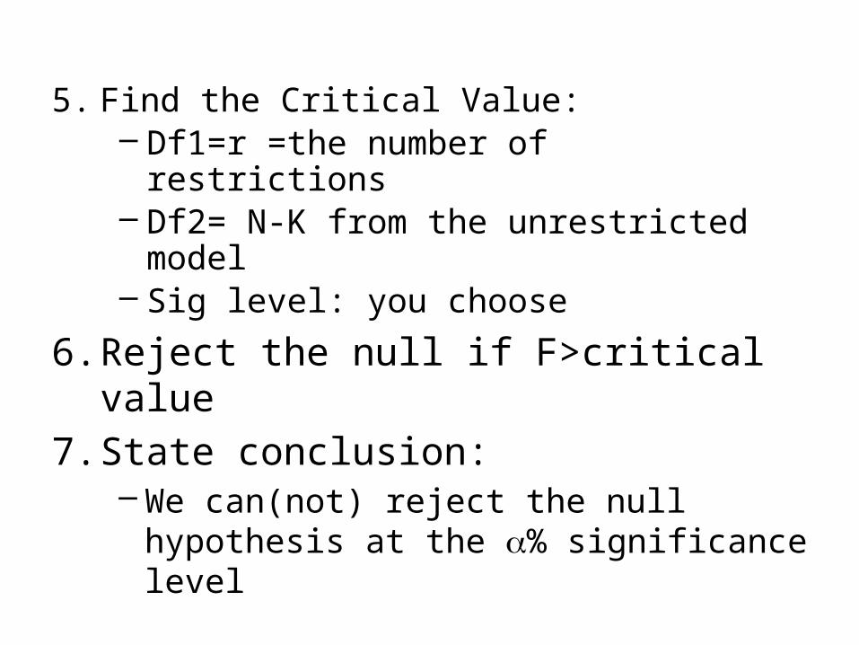
5. Find the Critical Value: – Df1=r =the number of restrictions– Df2= N-K from the unrestricted model– Sig level: you choose

6. Reject the null if F>critical value

7. State conclusion: – We can(not) reject the null hypothesis at the a% significance level

The Housing Example

1. H0: bH = 0 & bI= 1 H1: bH ≠ 0 or bI ≠1

2. RSSU= .11469849

3. RSSR= .193894893 (see over)

4. Calculate the test statistic =8.645. Critical value F(2,25) at 5% is 3.39

6. We can reject the null at the 5% significance level

The Restricted Model• To estimate the restricted model requires us

to impose the hypothesis on the model– i.e. treat the hypothesis as true and re-estimate

the model– This is true for a t-test also but trickier here

• The unrestricted model is:lpt = b0 + bI Linct + bH Lht +ut

• Imposing the restrictions giveslpt = b0 + 1* Linct + 0*Lht +ut

lpt - Linct = b0 + ut

• The zero restriction just means that the variable drops out

• A restriction that require coeff to be another number is more of a problem

• Trick is to bring it over to the LHS of equation

• We then generate a new variable for the right hand side and use that to estimate the restricted model

gen y=lprice-linc

. regress y if year<=1997

Source | SS df MS Number of obs = 28-------------+------------------------------ F( 0, 27) = 0.00 Model | 0 0 . Prob > F = . Residual | .193894893 27 .007181292 R-squared = 0.0000-------------+------------------------------ Adj R-squared = 0.0000 Total | .193894893 27 .007181292 Root MSE = .08474

------------------------------------------------------------------------------ y | Coef. Std. Err. t P>|t| [95% Conf. Interval]-------------+---------------------------------------------------------------- _cons | 1.884108 .0160148 117.65 0.000 1.851248 1.916968------------------------------------------------------------------------------

• Comment– This may seem like a silly regression after all it has no variables on the

right side (just the constant)– The regression is of no interest itself. – It is merely the regression of the original model with the restriction

imposed– The only thing we care about is the RSS (red)

Intuition of F-test

• Recall that the RSS is the variation in the Y variable that is not explained by the model

• The F-test compares the size of this unexplained bit before and after the restriction is imposed.

• If imposing the restriction causes the RSS to rise by a lot then that suggests that restriction is not supported by the data– model with the restriction explains a lot less of

the variation in Y

Intuition cont.

• Look at the formula for the test statistic– It is basically the %increase in RSS brought

about by the restriction– The % decline in explanatory power– The DF are just adjustments for statistical

reasons (ensure test has F distribution)• If the decline in explanatory power is large

enough we reject the null• How large?

– Larger than critical value

Comments on F• Almost any test can be formulated as linear restriction

– Very general method• T-test is a special case

– Exercise: reformulate a t-test as f-test• Test of joint significance is another special case• Stata: test command

– Use it to verify your results• Related to R2 – can reformulate the f-test in terms of R2

(see book)• Note that RSSR> RSSU

– A restriction cannot improve the fit of the model– The question is if the deterioration is large– F is always positive

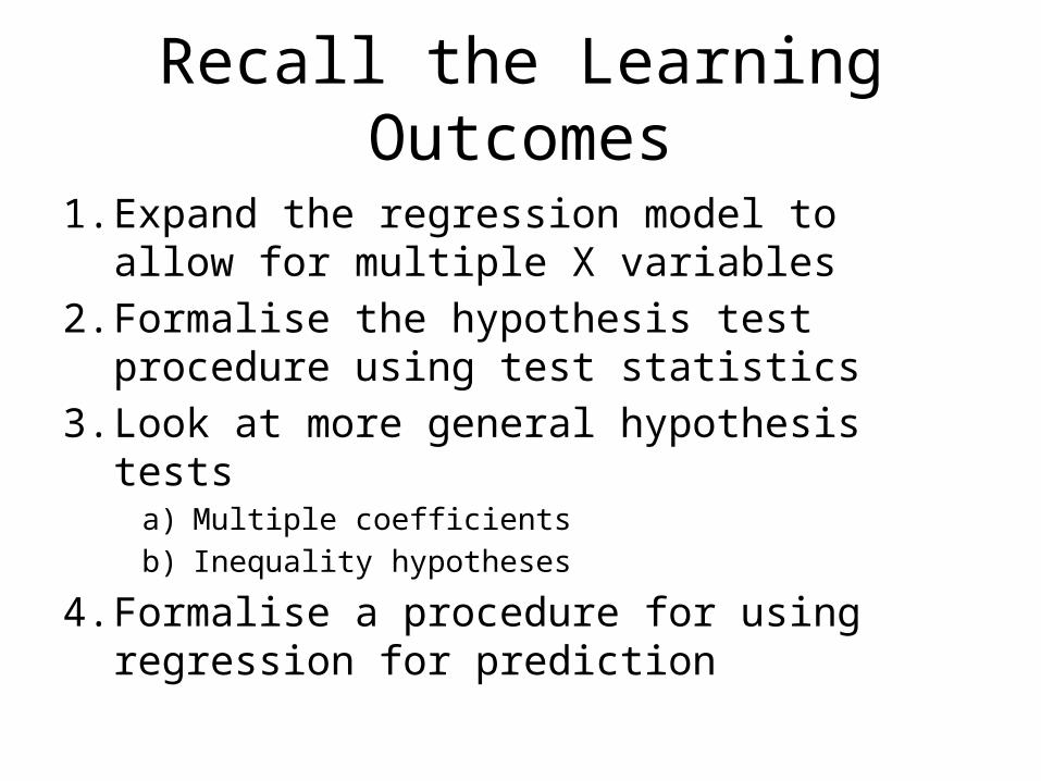
Recall the Learning Outcomes

1. Expand the regression model to allow for multiple X variables

2. Formalise the hypothesis test procedure using test statistics

3. Look at more general hypothesis testsa) Multiple coefficients

b) Inequality hypotheses

4. Formalise a procedure for using regression for prediction

What’s Next?

• We now have all we need to analyse many questions

• Next (quick) topic will be lawyers fees• But we are still missing two big items

– A discussion of the theory of why OLS gives good estimators

– A discussion of the circumstances which can lead to ols giving bad estimators.

• These will take up most of the rest of the course