This article was downloaded by: [George Mason University]On: 28 March 2014, At: 12:17Publisher: Taylor & FrancisInforma Ltd Registered in England and Wales Registered Number: 1072954 Registeredoffice: Mortimer House, 37-41 Mortimer Street, London W1T 3JH, UK

International Journal of Digital EarthPublication details, including instructions for authors andsubscription information:http://www.tandfonline.com/loi/tjde20

Integrating global land coverproducts for improved forest covercharacterization: an application inNorth AmericaXiao-Peng Songa, Chengquan Huanga, Min Fenga, Joseph O.Sextona, Saurabh Channana & John R. Townshenda

a Global Land Cover Facility, Department of GeographicalSciences, University of Maryland, College Park, MD, USAAccepted author version posted online: 22 Oct 2013.Publishedonline: 02 Dec 2013.

To cite this article: Xiao-Peng Song, Chengquan Huang, Min Feng, Joseph O. Sexton, SaurabhChannan & John R. Townshend (2013): Integrating global land cover products for improved forestcover characterization: an application in North America, International Journal of Digital Earth, DOI:10.1080/17538947.2013.856959

To link to this article: http://dx.doi.org/10.1080/17538947.2013.856959

PLEASE SCROLL DOWN FOR ARTICLE

Taylor & Francis makes every effort to ensure the accuracy of all the information (the“Content”) contained in the publications on our platform. Taylor & Francis, our agents,and our licensors make no representations or warranties whatsoever as to the accuracy,completeness, or suitability for any purpose of the Content. Versions of publishedTaylor & Francis and Routledge Open articles and Taylor & Francis and Routledge OpenSelect articles posted to institutional or subject repositories or any other third-partywebsite are without warranty from Taylor & Francis of any kind, either expressedor implied, including, but not limited to, warranties of merchantability, fitness for aparticular purpose, or non-infringement. Any opinions and views expressed in this articleare the opinions and views of the authors, and are not the views of or endorsed byTaylor & Francis. The accuracy of the Content should not be relied upon and should beindependently verified with primary sources of information. Taylor & Francis shall not beliable for any losses, actions, claims, proceedings, demands, costs, expenses, damages,and other liabilities whatsoever or howsoever caused arising directly or indirectly inconnection with, in relation to or arising out of the use of the Content.

This article may be used for research, teaching, and private study purposes. Anysubstantial or systematic reproduction, redistribution, reselling, loan, sub-licensing,systematic supply, or distribution in any form to anyone is expressly forbidden. Terms &Conditions of access and use can be found at http://www.tandfonline.com/page/terms-and-conditions

Taylor & Francis and Routledge Open articles are normally published under a CreativeCommons Attribution License http://creativecommons.org/licenses/by/3.0/. However,authors may opt to publish under a Creative Commons Attribution-Non-CommercialLicense http://creativecommons.org/licenses/by-nc/3.0/ Taylor & Francis and RoutledgeOpen Select articles are currently published under a license to publish, which is basedupon the Creative Commons Attribution-Non-Commercial No-Derivatives License, butallows for text and data mining of work. Authors also have the option of publishingan Open Select article under the Creative Commons Attribution License http://creativecommons.org/licenses/by/3.0/. It is essential that you check the license status of any given Open and OpenSelect article to confirm conditions of access and use.

Dow

nloa

ded

by [

Geo

rge

Mas

on U

nive

rsity

] at

12:

17 2

8 M

arch

201

4

Integrating global land cover products for improved forest covercharacterization: an application in North America

Xiao-Peng Song*, Chengquan Huang, Min Feng, Joseph O. Sexton, Saurabh Channanand John R. Townshend

Global Land Cover Facility, Department of Geographical Sciences, University of Maryland,College Park, MD, USA

(Received 18 June 2013; accepted 8 October 2013)

Six widely used coarse-resolution global land cover data-sets – Global Land CoverCharacterization (GLCC), Global Land Cover 2000 (GLC2000), GlobCover landcover product (GlobCover), MODIS land cover product (MODIS LC), the Universityof Maryland land cover product (UMD LC), and the MODIS Vegetation ContinuousFields tree cover layer (MODIS VCF) disagree substantially in their estimates of forestcover. Employing a regression tree model trained on higher-resolution, Landsat-baseddata, these multisource multiresolution maps were integrated for an improvedcharacterization of forest cover over North America. Evaluated using a withheld testsample, the integrated percent forest cover (IPFC) data-set has a root mean squareerror of 11.75% – substantially better than the 17.37% of GLCC, 17.61% ofGLC2000, 17.96% of GlobCover, 15.23% of MODIS LC, 19.25% of MODIS VCF,and 15.15% of UMD LC, respectively. Although demonstrated for forest, thisapproach based on integration of multiple products has potential for improvedcharacterization of other land cover types as well.

Keywords: land cover; forest; data fusion; regression tree; North America

1. Introduction

Satellite images have been used to characterize global patterns of land cover and land usesince the mid-1990s. Developed using different data-sets and different methodologies, sixglobal maps are now freely available at 300-m to 1-km resolutions: Global Land CoverCharacterization (GLCC) (Loveland et al. 2000), Global Land Cover 2000 (GLC2000)(Bartholomé and Belward 2005), GlobCover land cover product (GlobCover) (Bicheronet al. 2008), the Moderate Resolution Imaging Spectroradiometer land cover product(MODIS land cover product [MODIS LC]) (Friedl et al. 2002), the University ofMaryland land cover product (UMD LC) (Hansen et al. 2000), and the MODISVegetation Continuous Fields product (MODIS VCF) (Hansen et al. 2003).

A number of finer (e.g. Landsat-class) resolution land cover maps have also beengenerated from satellite data at regional to national scales (Hansen and Loveland, 2012),such as the North America Forest Disturbance product (Masek et al. 2008), the South

*Corresponding author. Email: xpsong@umd.edu

International Journal of Digital Earth, 2013

http://dx.doi.org/10.1080/17538947.2013.856959

© 2013 The Author(s). Published by Taylor & Francis.This is an Open Access article. Non-commercial re-use, distribution, and reproduction in any medium, provided the original workis properly attributed, cited, and is not altered, transformed, or built upon in any way, is permitted. The moral rights of the namedauthor(s) have been asserted.

Dow

nloa

ded

by [

Geo

rge

Mas

on U

nive

rsity

] at

12:

17 2

8 M

arch

201

4

Dakota State University Congo/Indonesia/European Russia forest cover and loss maps(Broich et al. 2011; Potapov, Turubanova, and Hansen 2011; Potapov et al. 2012); theUnited States Department of Agriculture Cropland Data Layer (USDA 2013); theBrazilian PRODES (Amazon Deforestation Monitoring Project) deforestation maps(INPE 2013), as well as the United States National Land Cover Dataset (NLCD) (Homeret al. 2004; Xian, Homer, and Fry 2009). Often derived with greater local expertise thanis possible with a global product, these regional Landsat-resolution data-sets provide amore accurate representation of the land surface type with greater spatial and thematicdetails. Some of these regional products have been well validated with finer-resolutionimagery or field data, e.g. NLCD has an overall accuracy of 85.3% (Wickham et al.2010). The accuracy of these regional data-sets has enabled their use as reference data fortraining or validating coarse-resolution products (Friedl et al. 2002; Hansen et al. 2003;Strahler et al. 2006).

Previous studies comparing sets of two or three of the existing global products foundgeneral, yet variable agreement among them (e.g. Defries and Townshend 1994; Fritz andSee 2008; Giri, Zhu, and Reed 2005; Hansen and Reed 2000; Herold et al. 2008; Junget al. 2006; Pflugmacher et al. 2011; Song et al. 2011). High agreement tends to belocated in relatively homogeneous and spectrally distinctive regions, whereas lowagreement tends to be located in heterogeneous landscapes, land cover transition zonesand in spectrally similar classes. Spatial patterns of agreement and disagreement revealedby cross-product comparison are useful for applications of these products; but ultimately,more accurate data-sets are always needed to meet users’ specific research demands. Yet,few attempts have been made to synthesize these data-sets into a consistent map. Junget al. (2006) collected multiple versions of GLC2000, GLCC, and MODIS LC andmerged them into a joint 1-km global land cover map by cross-walking different landcover legends. Fritz et al. (2011) created a hybrid cropland map for Africa using anapproach modified from Jung et al.’s (2006) synergy method by introducing an expertranking step and a calibration step with national cropland statistics. Similarly,Schepaschenko et al. (2011) produced a hybrid land cover data-set over Russia bycombing satellite-derived land cover maps, a Geographic Information System databaseand national statistics based on a set of knowledge rules.

Here we propose a supervised, harmonization-based method for integrating multi-resolution, multisource global products to improve land cover characterization. Todemonstrate this approach, we use the six global maps above-mentioned as input and oneLandsat-based map as reference to derive an integrated percent forest cover (IPFC) mapover North America. Our long-term goal is to generate an improved forest cover map atthe global scale to provide better parameterization for simulating land process in EarthSystem models (Lawrence and Chase 2007). Although we focus on the representation offorests in North America where we have sufficient reference data available for assessmentof our results, the approach derived through this study can potentially be applied to anylarge area and any other land cover type.

2. Data

We chose six widely used and available global data-sets to integrate. Each of these data-sets was derived based on moderate-resolution satellite imagery (Table 1). The GLCC andUMD LC were developed using a global Advanced Very High Resolution Radiometer(AVHRR) data-set (Townshend et al. 1994). The MODIS LC and MODIS VCF were

2 X.-P. Song et al.

Dow

nloa

ded

by [

Geo

rge

Mas

on U

nive

rsity

] at

12:

17 2

8 M

arch

201

4

derived using data from MODIS. Data from the Satellite Pour l’Observation de la Terre(SPOT-4) and Medium Resolution Imaging Spectrometer (MERIS) sensors were used toproduce the GLC2000 and GlobCover, respectively. It should be noted that in somecases, e.g. MODIS-derived products, multiple versions have been generated followingalgorithmic improvements (Friedl et al. 2002, 2010; Hansen et al. 2003, 2005). Theselection of the six global data-sets for this study takes into account several specificconsiderations: UMD LC and GLCC were the first 1-km maps generated; both MODISLC and MODIS VCF are standard MODIS land products; MODIS VCF is a fractionalland cover map; and GlobCover has the finest spatial resolution at the global scale.Collectively, these six maps represent land cover data-sets in different legends, derivedfrom different sensor systems and with diverse classification approaches (Table 1).

We use the Landsat-based National Land Cover Database 2001 (NLCD2001) over theconterminous United States as a reference for model training and product evaluation(Homer et al. 2004). Validated against expert-interpreted 1-m Digital Orthophoto QuarterQuadrangles, the NLCD2001 has 87% user’s accuracy and 88.5% producer’s accuracy forthe forest class (Wickham et al. 2010). Further details of NLCD2001 are provided inTable 1 and associated references.

3. Method

The data integration method consists of a series of steps (Figure 1) described in each ofthe sections below. As a preprocessing step, all products were reprojected to LambertAzimuthal Equal Area projection with the WGS84 datum. They were also registered to acommon spatial extent using nearest neighbor resampling.

3.1. Standardization to a common spatial and thematic scale

These various data-sets need to be standardized to a common spatial and thematic scaleprior to integration. We first defined a set of translation rules to convert each categorical

Table 1. Summary of land cover products used in this study.

Product Sensor Date ResolutionClassificationapproach Publication

GLCC AVHRR April 1992–March 1993

1-km Clustering –Labeling

Lovelandet al. (2000)

GLC2000 SPOT-4 November 1999–December 2000

1-km Depends onindividual region

Bartholomé andBelward (2005)

GlobCover MERIS December 2004–June 2006

300-m Supervised andunsupervised

Bicheronet al. (2008)

MODISLC

MODIS October 2000–October 2001

1-km Decision tree Friedlet al. (2002)

MODISVCF

MODIS October 2000–December 2001

500-m Regression tree Hansenet al. (2003)

UMD LC AVHRR April 1992–March 1993

1-km Decision tree Hansenet al. (2000)

NLCD2001 Landsat5 & 7

Circa 2001 30-m Decision tree Homeret al. (2004)

International Journal of Digital Earth 3

Dow

nloa

ded

by [

Geo

rge

Mas

on U

nive

rsity

] at

12:

17 2

8 M

arch

201

4

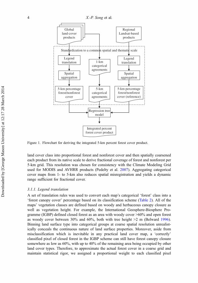
land cover class into proportional forest and nonforest cover and then spatially coarsenedeach product from its native scale to derive fractional coverage of forest and nonforest per5-km grid. This resolution was chosen for consistency with the Climate Modeling Gridused for MODIS and AVHRR products (Pedelty et al. 2007). Aggregating categoricalcover maps from 1- to 5-km also reduces spatial misregistration and yields a dynamicrange sufficient for fractional cover.

3.1.1. Legend translation

A set of translation rules was used to convert each map’s categorical ‘forest’ class into a‘forest canopy cover’ percentage based on its classification scheme (Table 2). All of themaps’ vegetation classes are defined based on woody and herbaceous canopy closure aswell as vegetation height. For example, the International Geosphere-Biosphere Pro-gramme (IGBP) defined closed forest as an area with woody cover >60% and open forestas woody cover between 30% and 60%, both with tree height >2 m (Belward 1996).Binning land surface type into categorical groups at coarse spatial resolution unrealist-ically conceals the continuous nature of land surface properties. Moreover, aside frommisclassification which is inevitable in any practical land cover map, a ‘correctly’classified pixel of closed forest in the IGBP scheme can still have forest canopy closuresomewhere as low as 60%, with up to 40% of the remaining area being occupied by otherland cover types. Therefore, to approximate the actual forest cover in a coarse grid andmaintain statistical rigor, we assigned a proportional weight to each classified pixel

Global land-cover products

Regional Landsat-based

products

Legend translation

Spatial aggregation

Legend translation

Spatial aggregation

Regression treemodel

Integrated percent forest cover product

5-km percentage forest/nonforest

cover

5-km percentage forest/nonforest cover (reference)

1-km categorical agreements

5-km categorical agreements

Standardization to a common spatial and thematic scale

Figure 1. Flowchart for deriving the integrated 5-km percent forest cover product.

4 X.-P. Song et al.

Dow

nloa

ded

by [

Geo

rge

Mas

on U

nive

rsity

] at

12:

17 2

8 M

arch

201

4

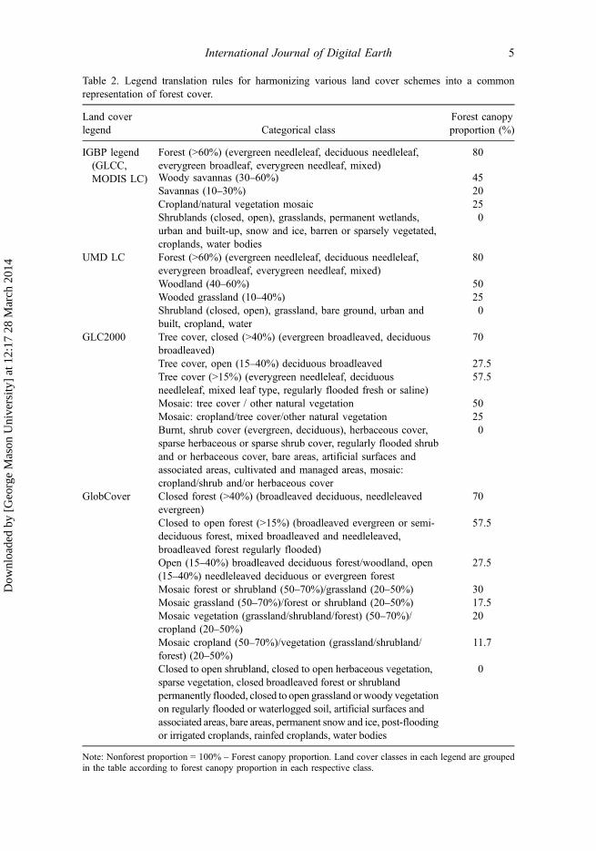
Table 2. Legend translation rules for harmonizing various land cover schemes into a commonrepresentation of forest cover.

Land coverlegend Categorical class

Forest canopyproportion (%)

IGBP legend(GLCC,MODIS LC)

Forest (>60%) (evergreen needleleaf, deciduous needleleaf,everygreen broadleaf, everygreen needleaf, mixed)

80

Woody savannas (30–60%) 45Savannas (10–30%) 20Cropland/natural vegetation mosaic 25Shrublands (closed, open), grasslands, permanent wetlands,urban and built-up, snow and ice, barren or sparsely vegetated,croplands, water bodies

0

UMD LC Forest (>60%) (evergreen needleleaf, deciduous needleleaf,everygreen broadleaf, everygreen needleaf, mixed)

80

Woodland (40–60%) 50Wooded grassland (10–40%) 25Shrubland (closed, open), grassland, bare ground, urban andbuilt, cropland, water

0

GLC2000 Tree cover, closed (>40%) (evergreen broadleaved, deciduousbroadleaved)

70

Tree cover, open (15–40%) deciduous broadleaved 27.5Tree cover (>15%) (everygreen needleleaf, deciduousneedleleaf, mixed leaf type, regularly flooded fresh or saline)

57.5

Mosaic: tree cover / other natural vegetation 50Mosaic: cropland/tree cover/other natural vegetation 25Burnt, shrub cover (evergreen, deciduous), herbaceous cover,sparse herbaceous or sparse shrub cover, regularly flooded shruband or herbaceous cover, bare areas, artificial surfaces andassociated areas, cultivated and managed areas, mosaic:cropland/shrub and/or herbaceous cover

0

GlobCover Closed forest (>40%) (broadleaved deciduous, needleleavedevergreen)

70

Closed to open forest (>15%) (broadleaved evergreen or semi-deciduous forest, mixed broadleaved and needleleaved,broadleaved forest regularly flooded)

57.5

Open (15–40%) broadleaved deciduous forest/woodland, open(15–40%) needleleaved deciduous or evergreen forest

27.5

Mosaic forest or shrubland (50–70%)/grassland (20–50%) 30Mosaic grassland (50–70%)/forest or shrubland (20–50%) 17.5Mosaic vegetation (grassland/shrubland/forest) (50–70%)/cropland (20–50%)

20

Mosaic cropland (50–70%)/vegetation (grassland/shrubland/forest) (20–50%)

11.7

Closed to open shrubland, closed to open herbaceous vegetation,sparse vegetation, closed broadleaved forest or shrublandpermanently flooded, closed to open grassland orwoody vegetationon regularly flooded or waterlogged soil, artificial surfaces andassociated areas, bare areas, permanent snow and ice, post-floodingor irrigated croplands, rainfed croplands, water bodies

0

Note: Nonforest proportion = 100% – Forest canopy proportion. Land cover classes in each legend are groupedin the table according to forest canopy proportion in each respective class.

International Journal of Digital Earth 5

Dow

nloa

ded

by [

Geo

rge

Mas

on U

nive

rsity

] at

12:

17 2

8 M

arch

201

4

corresponding to the mean value of its woody canopy closure as defined in its originallegend, e.g. 80% to closed forest and 45% to open forest for the IGBP legend (Table 2).Classes such as closed and open shrublands, croplands, grasslands, permanent wetlands,urban and built-up, snow and ice, bare, and water bodies do not contain any forest cover.Thus, they were assigned a 0% forest cover and 100% nonforest cover. The mosaic classesin different land cover legends raise challenges in any legend harmonization work (Junget al. 2006). The cropland/natural vegetation mosaic class in the IGBP legend contains amixture of four classes including croplands, forests, shrublands, and grasslands (Belward1996), so it was split into 25% forest cover and 75% nonforest cover. The complete legendtranslation rule set is given in Table 2. With these rules, each land cover product wasconverted to a percent forest cover map at its native resolution. MODIS VCF directlygives percent canopy cover for each pixel and hence no further translation is needed.

3.1.2. Spatial aggregation

Each percent forest cover map was overlaid on the 5-km grid to calculate percent coverwithin each 5-km grid cell. For example, for the 1-km categorical GLCC, the aggregationwas carried out by employing a 5×5 pixel window moving across the map. Within thelocal window, each classified pixel was first multiplied by its class-specific proportionalweight defined by the legend translation rule, and then averaged to derive theproportional forest and nonforest cover within the 5-km grid. Other categorical mapswere aggregated in the same way as GLCC. As MODIS VCF directly measures thepercentage of forest canopy, we simply aggregated it from 500-m to 5-km with a 10×10local moving window by averaging the 100 pixel values within the window.

3.1.3. Deriving forest agreement metrics

At the pixel level, it is reasonable to believe that a given land pixel is more likely to beforest if all six products independently classify the pixel as forest than if only one productidentifies it as forest and the other five products label it as nonforest. Thus, differentlevels of agreement reflect varying degrees of certainty regarding the true forest cover inone pixel. In order to directly incorporate this agreement information into dataintegration, we calculated the pixel-based agreement metrics for the forest class. Thisanalysis is based on categorical maps in parallel with the above legend translation andspatial aggregation process. As four of the six input products (i.e. GLCC, GLC2000,MODIS LC, and UMD LC) have an original resolution of 1-km, we first align all the sixproducts at 1-km resolution to calculate a 1-km forest ‘vote’ map and then derive the5-km agreement metrics based upon the 1-km vote map. The 300-m GlobCover wasresampled to 1-km resolution and the 500-m fractional MODIS VCF was spatiallyaveraged to 1-km first and converted to binary forest and nonforest by applying a 30%threshold according to the IGBP definition.

To assess the degree of correspondence between the six products at 1-km, weevaluated each pixel as the number of times it was labeled as forest by the six maps,resulting in a value between 0 and 6: the higher the value, the higher the agreementbetween the products for the forest class. The 5-km agreement metrics were derived bygrouping the 1-km metrics using a 5×5 pixel moving window. Within the local window,the 1-km agreement pixels with values between 0 and 6 were noted and each 5-km gridwas characterized by the frequencies of each of those values. Each 5-km grid thencorresponds to the frequency histogram of 0–6 for forest agreement at 1-km resolution.

6 X.-P. Song et al.

Dow

nloa

ded

by [

Geo

rge

Mas

on U

nive

rsity

] at

12:

17 2

8 M

arch

201

4

3.2. Supervized training and prediction

A supervized regression tree algorithm was used to model the relationship betweenreference cover values from NLCD2001 and forest cover values as well as agreementmetrics from the coarse data-sets. Tree-based classification and regression methods arewell established in land cover characterization studies (e.g. Friedl et al. 2002; Hansenet al. 2003, 2000; Homer et al. 2004; Sexton et al. 2013a, 2013b; Xian and Crane 2005).Regression trees have the theoretical advantage of handling nonlinear relationships byrecursively splitting the sample into binary partitions until criteria of accuracy or purityare met (Breiman et al. 1984). This algorithm produces a hierarchical set of decisionrules, each of which terminates in a linear regression model. Predictor variables feedinginto the regression tree model consist of the proportional forest and nonforest cover layersderived through legend translation and spatial aggregation. The seven agreement metricslayers are used in the conditional statements of the regression rules to parameterize thetree model. Reference data were derived by aggregating NLCD2001 from 30-m to5-km resolution to calculate the percentage of forest pixels per 5-km grid. A total of40,713 pixels (∼12% of land pixels) were systematically selected from the aggregatedNLCD2001, from which half were randomly selected for model training and half for datavalidation.

3.3. Product evaluation

Accuracies of the six input data-sets and the output IPFC data-set were evaluated againstthe aggregated NLCD2001 values using mean bias error (MBE), root mean square error(RMSE) and r2:

MBE ¼Pn

i¼1 ðPi � RiÞn

ð1Þ

RMSE ¼ffiffiffiffiffiffiffiffiffiffiffiffiffiffiffiffiffiffiffiffiffiffiffiffiffiffiffiffiffiffiffiPn

i¼1 ðPi � RiÞn

2s

ð2Þ

r2 ¼ 1�Pn

i¼1 Pi � Rið Þ2Pni¼1 Ri � R

� �2 , ð3Þ

where i is the sample index; Pi is the value of IPFC or forest cover of each input product;Ri is the reference forest cover per sample; R is the mean of reference; and n is the samplesize (Willmott 1982). The test sample was further divided according to reference valuesinto three subsets representing low, moderate, and high forest cover (i.e. 0–30%, 31–60%,61–100%), respectively. Accuracy metrics were calculated using the entire test sample aswell as these three subsets to report the disaggregate error by categories of percent forestcover.

4. Results

4.1. Model fitting and performance assessment

Evaluation of the regression tree model using 20,357 training cases yielded an averageerror of 6.46% with a correlation coefficient between reference and predicted cover of0.94. Internal 10-fold cross-validation on training data estimated a slightly higher average

International Journal of Digital Earth 7

Dow

nloa

ded

by [

Geo

rge

Mas

on U

nive

rsity

] at

12:

17 2

8 M

arch

201

4

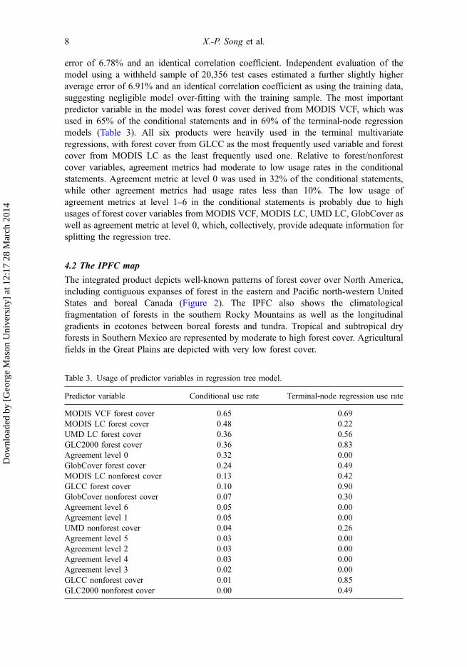
error of 6.78% and an identical correlation coefficient. Independent evaluation of themodel using a withheld sample of 20,356 test cases estimated a further slightly higheraverage error of 6.91% and an identical correlation coefficient as using the training data,suggesting negligible model over-fitting with the training sample. The most importantpredictor variable in the model was forest cover derived from MODIS VCF, which wasused in 65% of the conditional statements and in 69% of the terminal-node regressionmodels (Table 3). All six products were heavily used in the terminal multivariateregressions, with forest cover from GLCC as the most frequently used variable and forestcover from MODIS LC as the least frequently used one. Relative to forest/nonforestcover variables, agreement metrics had moderate to low usage rates in the conditionalstatements. Agreement metric at level 0 was used in 32% of the conditional statements,while other agreement metrics had usage rates less than 10%. The low usage ofagreement metrics at level 1–6 in the conditional statements is probably due to highusages of forest cover variables from MODIS VCF, MODIS LC, UMD LC, GlobCover aswell as agreement metric at level 0, which, collectively, provide adequate information forsplitting the regression tree.

4.2 The IPFC map

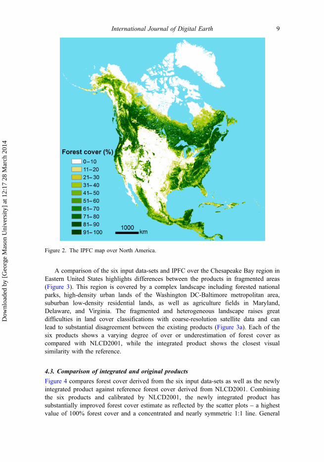
The integrated product depicts well-known patterns of forest cover over North America,including contiguous expanses of forest in the eastern and Pacific north-western UnitedStates and boreal Canada (Figure 2). The IPFC also shows the climatologicalfragmentation of forests in the southern Rocky Mountains as well as the longitudinalgradients in ecotones between boreal forests and tundra. Tropical and subtropical dryforests in Southern Mexico are represented by moderate to high forest cover. Agriculturalfields in the Great Plains are depicted with very low forest cover.

Table 3. Usage of predictor variables in regression tree model.

Predictor variable Conditional use rate Terminal-node regression use rate

MODIS VCF forest cover 0.65 0.69MODIS LC forest cover 0.48 0.22UMD LC forest cover 0.36 0.56GLC2000 forest cover 0.36 0.83Agreement level 0 0.32 0.00GlobCover forest cover 0.24 0.49MODIS LC nonforest cover 0.13 0.42GLCC forest cover 0.10 0.90GlobCover nonforest cover 0.07 0.30Agreement level 6 0.05 0.00Agreement level 1 0.05 0.00UMD nonforest cover 0.04 0.26Agreement level 5 0.03 0.00Agreement level 2 0.03 0.00Agreement level 4 0.03 0.00Agreement level 3 0.02 0.00GLCC nonforest cover 0.01 0.85GLC2000 nonforest cover 0.00 0.49

8 X.-P. Song et al.

Dow

nloa

ded

by [

Geo

rge

Mas

on U

nive

rsity

] at

12:

17 2

8 M

arch

201

4

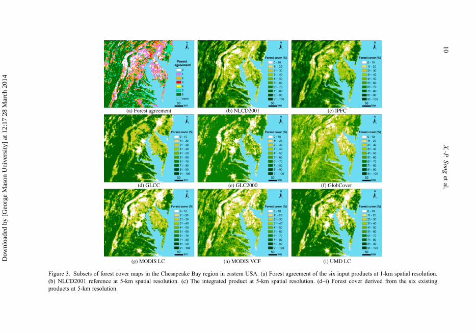
A comparison of the six input data-sets and IPFC over the Chesapeake Bay region inEastern United States highlights differences between the products in fragmented areas(Figure 3). This region is covered by a complex landscape including forested nationalparks, high-density urban lands of the Washington DC-Baltimore metropolitan area,suburban low-density residential lands, as well as agriculture fields in Maryland,Delaware, and Virginia. The fragmented and heterogeneous landscape raises greatdifficulties in land cover classifications with coarse-resolution satellite data and canlead to substantial disagreement between the existing products (Figure 3a). Each of thesix products shows a varying degree of over or underestimation of forest cover ascompared with NLCD2001, while the integrated product shows the closest visualsimilarity with the reference.

4.3. Comparison of integrated and original products

Figure 4 compares forest cover derived from the six input data-sets as well as the newlyintegrated product against reference forest cover derived from NLCD2001. Combiningthe six products and calibrated by NLCD2001, the newly integrated product hassubstantially improved forest cover estimate as reflected by the scatter plots – a highestvalue of 100% forest cover and a concentrated and nearly symmetric 1:1 line. General

Figure 2. The IPFC map over North America.

International Journal of Digital Earth 9

Dow

nloa

ded

by [

Geo

rge

Mas

on U

nive

rsity

] at

12:

17 2

8 M

arch

201

4

(a) Forest agreement (b) NLCD2001 (c) IPFC

(d) GLCC (e) GLC2000 (f) GlobCover

(g) MODIS LC (h) MODIS VCF (i) UMD LC

Figure 3. Subsets of forest cover maps in the Chesapeake Bay region in eastern USA. (a) Forest agreement of the six input products at 1-km spatial resolution.(b) NLCD2001 reference at 5-km spatial resolution. (c) The integrated product at 5-km spatial resolution. (d–i) Forest cover derived from the six existingproducts at 5-km resolution.

10X.-P.

Songet

al.

Dow

nloa

ded

by [

Geo

rge

Mas

on U

nive

rsity

] at

12:

17 2

8 M

arch

201

4

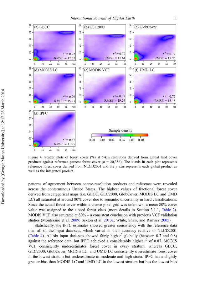
patterns of agreement between coarse-resolution products and reference were revealedacross the conterminous United States. The highest values of fractional forest coverderived from categorical maps (i.e. GLCC, GLC2000, GlobCover, MODIS LC and UMDLC) all saturated at around 80% cover due to semantic uncertainty in hard classifications.Since the actual forest cover within a coarse pixel grid was unknown, a mean 80% covervalue was assigned to the closed forest class (more details in Section 3.1.1, Table 2).MODIS VCF also saturated at 80% – a consistent conclusion with previous VCF validationstudies (Montesano et al. 2009; Sexton et al. 2013a; White, Shaw, and Ramsey 2005).

Statistically, the IPFC estimates showed greater consistency with the reference datathan all of the input data-sets, which varied in their accuracy relative to NLCD2001(Table 4). All six input data-sets showed fairly high r2 globally (between 0.7 and 0.8)against the reference data, but IPFC achieved a considerably higher r2 of 0.87. MODISVCF consistently underestimates forest cover in every stratum, whereas GLCC,GLC2000, GlobCover, MODIS LC, and UMD LC consistently overestimate forest coverin the lowest stratum but underestimate in moderate and high strata. IPFC has a slightlygreater bias than MODIS LC and UMD LC in the lowest stratum but has the lowest bias

Figure 4. Scatter plots of forest cover (%) at 5-km resolution derived from global land coverproducts against reference percent forest cover (n = 20,356). The x axis in each plot representsreference forest cover derived from NLCD2001 and the y axis represents each global product aswell as the integrated product.

International Journal of Digital Earth 11

Dow

nloa

ded

by [

Geo

rge

Mas

on U

nive

rsity

] at

12:

17 2

8 M

arch

201

4

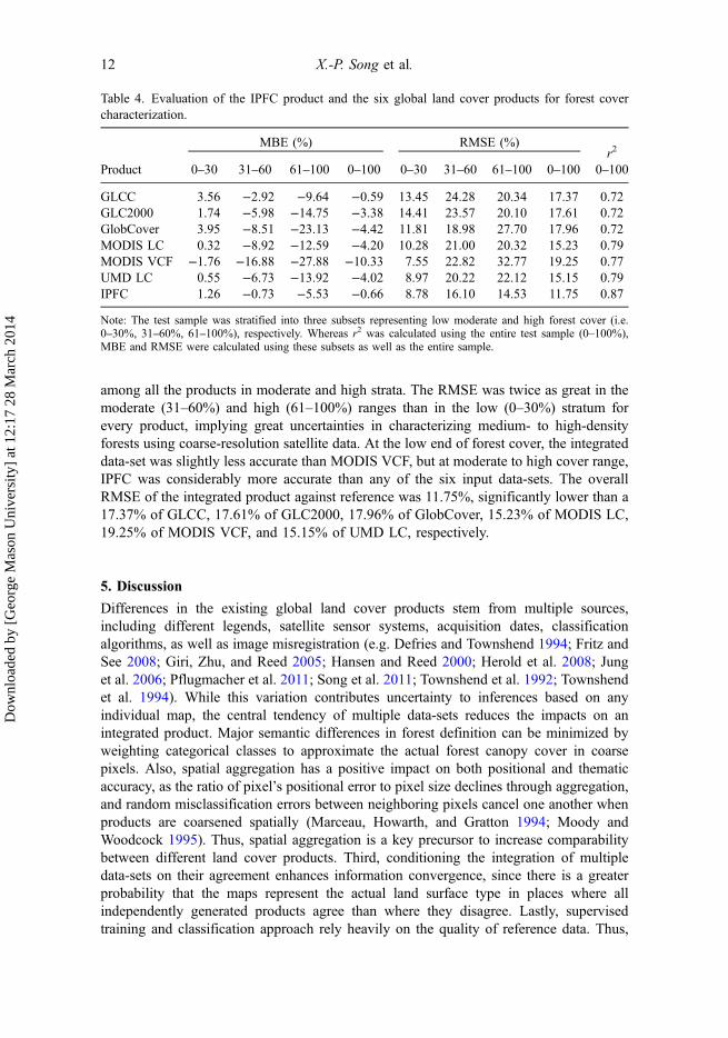
among all the products in moderate and high strata. The RMSE was twice as great in themoderate (31–60%) and high (61–100%) ranges than in the low (0–30%) stratum forevery product, implying great uncertainties in characterizing medium- to high-densityforests using coarse-resolution satellite data. At the low end of forest cover, the integrateddata-set was slightly less accurate than MODIS VCF, but at moderate to high cover range,IPFC was considerably more accurate than any of the six input data-sets. The overallRMSE of the integrated product against reference was 11.75%, significantly lower than a17.37% of GLCC, 17.61% of GLC2000, 17.96% of GlobCover, 15.23% of MODIS LC,19.25% of MODIS VCF, and 15.15% of UMD LC, respectively.

5. Discussion

Differences in the existing global land cover products stem from multiple sources,including different legends, satellite sensor systems, acquisition dates, classificationalgorithms, as well as image misregistration (e.g. Defries and Townshend 1994; Fritz andSee 2008; Giri, Zhu, and Reed 2005; Hansen and Reed 2000; Herold et al. 2008; Junget al. 2006; Pflugmacher et al. 2011; Song et al. 2011; Townshend et al. 1992; Townshendet al. 1994). While this variation contributes uncertainty to inferences based on anyindividual map, the central tendency of multiple data-sets reduces the impacts on anintegrated product. Major semantic differences in forest definition can be minimized byweighting categorical classes to approximate the actual forest canopy cover in coarsepixels. Also, spatial aggregation has a positive impact on both positional and thematicaccuracy, as the ratio of pixel’s positional error to pixel size declines through aggregation,and random misclassification errors between neighboring pixels cancel one another whenproducts are coarsened spatially (Marceau, Howarth, and Gratton 1994; Moody andWoodcock 1995). Thus, spatial aggregation is a key precursor to increase comparabilitybetween different land cover products. Third, conditioning the integration of multipledata-sets on their agreement enhances information convergence, since there is a greaterprobability that the maps represent the actual land surface type in places where allindependently generated products agree than where they disagree. Lastly, supervisedtraining and classification approach rely heavily on the quality of reference data. Thus,

Table 4. Evaluation of the IPFC product and the six global land cover products for forest covercharacterization.

MBE (%) RMSE (%)r2

Product 0–30 31–60 61–100 0–100 0–30 31–60 61–100 0–100 0–100

GLCC 3.56 −2.92 −9.64 −0.59 13.45 24.28 20.34 17.37 0.72GLC2000 1.74 −5.98 −14.75 −3.38 14.41 23.57 20.10 17.61 0.72GlobCover 3.95 −8.51 −23.13 −4.42 11.81 18.98 27.70 17.96 0.72MODIS LC 0.32 −8.92 −12.59 −4.20 10.28 21.00 20.32 15.23 0.79MODIS VCF −1.76 −16.88 −27.88 −10.33 7.55 22.82 32.77 19.25 0.77UMD LC 0.55 −6.73 −13.92 −4.02 8.97 20.22 22.12 15.15 0.79IPFC 1.26 −0.73 −5.53 −0.66 8.78 16.10 14.53 11.75 0.87

Note: The test sample was stratified into three subsets representing low moderate and high forest cover (i.e.0–30%, 31–60%, 61–100%), respectively. Whereas r2 was calculated using the entire test sample (0–100%),MBE and RMSE were calculated using these subsets as well as the entire sample.

12 X.-P. Song et al.

Dow

nloa

ded

by [

Geo

rge

Mas

on U

nive

rsity

] at

12:

17 2

8 M

arch

201

4

collecting accurate and representative training data is critically important in generating aland cover product. Future high-quality Landsat-resolution data-sets such as Food andAgriculture Organization’s remote sensing survey Landsat sampling blocks (Potapovet al. 2011) would be candidate reference sources to the integration approachproposed here.

6. Summary

Global land cover products show substantial discrepancies in their representation of landsurface type, including forests. We present a data fusion method to integrate existingmultiresolution (e.g. 300-m to 1-km) multisource global land cover maps to derive a newhybrid product for the forest class, and we demonstrate the approach over North America.Different from previous data fusion methodologies by Jung et al. (2006) and Fritz et al.(2011), which mainly rely on agreement between different land cover products, ourapproach also uses a large sample of higher-resolution land cover data as reference tointegrate coarser data-sets in a supervised modeling framework. Compatible withprevious work, land cover characterization is greatly improved by combing varioussources of existing data-sets. Assessment of errors relative to a withheld test samplesuggests that the integrated forest map has an overestimation in low forest cover stratum(i.e. 0–30%) and a slight underestimation in moderate (i.e. 31–60%) to high forest coverstrata (i.e. 61–100%). Compared to the existing individual global maps of forest cover, aconsiderable improvement is achieved through data integration with an overall RMSE of11.75% against Landsat reference and, the greatest improvements are achieved inmoderate to high forest cover regions. This data-set is freely available for download at theGlobal Land Cover Facility (www.landcover.org).

AcknowledgmentsWe thank the anonymous reviewers for their valuable comments on the paper.

FundingThis study is a contribution to the Global Forest Cover Change project funded by NASA’sMaking Earth System Data Records for Use in Research Environments (MEaSUREs) Program[NNX08AP33A]. Additional support is provided by the NASA Earth and Space Science Fellowship(NESSF) Program [NNX12AN92H]; the Land-Cover/Land-Use Change Program[NNH07ZDA001N]; the Earth System Science from EOS Program [NNH06ZDA001N]; and theMODIS Science Team.

ReferencesBartholomé, E., and A. S. Belward. 2005. “GLC2000: A New Approach to Global Land Cover

Mapping from Earth Observation Data.” International Journal of Remote Sensing 26 (9): 1959–1977. doi:10.1080/01431160412331291297.

Belward, A. S. 1996. The IGBP-DIS Global 1 km Land Cover Data Set “DISCover”: Proposal andImplementation Plans. Report of the Land Cover Working Group of IGBP-DIS. Toulouse: IGBP-DIS Office.

Bicheron, P., P. Defourny, C. Brockmann, L. Schouten, C. Vancutsem, M. Huc, S. Bontemps, et al.2008. GlobCover: Products Description and Validation Report. Toulouse: Medias France.

Breiman, L., J. H. Friedman, R. A. Olshen, and C. J. Stone. 1984. Classification and RegressionTrees. Boca Raton, FL: Chapman & Hall/CRC.

Broich, M., M. C. Hansen, P. Potapov, B. Adusei, E. Lindquist, and S. V. Stehman. 2011. “Time-series Analysis of Multi-resolution Optical Imagery for Quantifying Forest Cover Loss in

International Journal of Digital Earth 13

Dow

nloa

ded

by [

Geo

rge

Mas

on U

nive

rsity

] at

12:

17 2

8 M

arch

201

4

Sumatra and Kalimantan, Indonesia.” International Journal of Applied Earth Observation andGeoinformation 13 (2): 277–291. doi:10.1016/j.jag.2010.11.004.

Defries, R. S., and J. R. G. Townshend. 1994. “NDVI-Derived Land-Cover Classifications at aGlobal-Scale.” International Journal of Remote Sensing 15 (17): 3567–3586. doi:10.1080/01431169408954345.

Friedl, M. A., D. K. McIver, J. C. F. Hodges, X. Y. Zhang, D. Muchoney, A. H. Strahler,C. E. Woodcock, et al. 2002. “Global Land Cover Mapping from MODIS: Algorithms andEarly Results.” Remote Sensing of Environment 83 (1–2): 287–302. doi:10.1016/S0034-4257(02)00078-0.

Friedl, M. A., D. Sulla-Menashe, B. Tan, A. Schneider, N. Ramankutty, A. Sibley, and X. Huang.2010. “MODIS Collection 5 Global Land Cover: Algorithm Refinements and Characterizationof New Datasets.” Remote Sensing of Environment 114 (1): 168–182. doi:10.1016/j.rse.2009.08.016.

Fritz, S., and L. See. 2008. “Identifying and Quantifying Uncertainty and Spatial Disagreement inthe Comparison of Global Land Cover for Different Applications.” Global Change Biology14 (5): 1057–1075. doi:10.1111/j.1365-2486.2007.01519.x.

Fritz, S., L. You, A. Bun, L. See, I. McCallum, C. Schill, C. Perger, J. Liu, M. Hansen, andM. Obersteiner. 2011. “Cropland for Sub-Saharan Africa: A Synergistic Approach Using Five LandCover Data Sets.” Geophysical Research Letters 38 (4): L04404. doi:10.1029/2010GL046213.

Giri, C., Z. Zhu, and B. Reed. 2005. “A Comparative Analysis of the Global Land Cover 2000 andMODIS Land Cover Data Sets.” Remote Sensing of Environment 94 (1): 123–132. doi:10.1016/j.rse.2004.09.005.

Hansen, M. C., and T. R. Loveland. 2012. “A Review of Large Area Monitoring of Land CoverChange Using Landsat Data.” Remote Sensing of Environment 122: 66–66. doi:10.1016/j.rse.2011.08.024.

Hansen, M. C., and B. Reed. 2000. “A Comparison of the IGBP DISCover and University ofMaryland 1 Km Global Land Cover Products.” International Journal of Remote Sensing21 (6–7): 1365–1373. doi:10.1080/014311600210218.

Hansen, M. C., R. S. DeFries, J. R. G. Townshend, M. Carroll, C. Dimiceli, and R. A. Sohlberg2003. “Global Percent Tree Cover at a Spatial Resolution of 500 Meters: First Results of theMODIS Vegetation Continuous Fields Algorithm.” Earth Interactions 7 (10): 1–15. doi:10.1175/1087-3562(2003)007<0001:GPTCAA>2.0.CO;2.

Hansen, M. C., R. S. DeFries, J. R. G. Townshend, and R. Sohlberg. 2000. “Global Land CoverClassification at 1 km Spatial Resolution Using a Classification Tree Approach.” InternationalJournal of Remote Sensing 21 (6–7): 1331–1364. doi:10.1080/014311600210209.

Hansen, M. C., J. R. G. Townshend, R. S. DeFries, and M. Carroll. 2005. “Estimation of TreeCover Using MODIS Data at Global, Continental and Regional/Local Scales.” InternationalJournal of Remote Sensing 26 (19): 4359–4380. doi:10.1080/01431160500113435.

Herold, M., P. Mayaux, C. E. Woodcock, A. Baccini, and C. Schmullius. 2008. “Some Challengesin Global Land Cover Mapping: An Assessment of Agreement and Accuracy in Existing 1 KmDatasets.” Remote Sensing of Environment 112 (5): 2538–2556. doi:10.1016/j.rse.2007.11.013.

Homer, C., C. Huang, L. Yang, B. Wylie, and M. Coan. 2004. “Development of a 2001 NationalLand-Cover Database for the United States.” Photogrammetric Engineering & Remote Sensing70: 829–840.

INPE. 2013. “Prodes Digital.” Accessed August 23. http://www.obt.inpe.br/prodes/index.phpJung, M., K. Henkel, M. Herold, and G. Churkina. 2006. “Exploiting Synergies of Global Land

Cover Products for Carbon Cycle Modeling.” Remote Sensing of Environment 101 (4): 534–553.doi:10.1016/j.rse.2006.01.020.

Lawrence, P. J., and T. N. Chase. 2007. “Representing a New MODIS Consistent Land Surface inthe Community Land Model (CLM 3.0).” Journal of Geophysical Research 112: 1–17.

Loveland, T. R., B. C. Reed, J. F. Brown, D. O. Ohlen, Z. Zhu, L. Yang, and J. W. Merchant. 2000.“Development of a Global Land Cover Characteristics Database and IGBP DISCover from 1 KmAVHRR Data.” International Journal of Remote Sensing 21 (6–7): 1303–1330. doi:10.1080/014311600210191.

Marceau, D. J., P. J. Howarth, and D. J. Gratton. 1994. “Remote Sensing and the Measurement ofGeographical Entities in a Forested Environment. 1. The Scale and Spatial AggregationProblem.” Remote Sensing of Environment 49 (2): 93–104. doi:10.1016/0034-4257(94)90046-9.

14 X.-P. Song et al.

Dow

nloa

ded

by [

Geo

rge

Mas

on U

nive

rsity

] at

12:

17 2

8 M

arch

201

4

Masek, J. G., C. Huang, R. Wolfe, W. Cohen, F. Hall, J. Kutler, and P. Nelson. 2008. “NorthAmerican Forest Disturbance Mapped from a Decadal Landsat Record.” Remote Sensing ofEnvironment 112 (6): 2914–2926. doi:10.1016/j.rse.2008.02.010.

Montesano, P. M., R. Nelson, G. Sun, H. Margolis, A. Kerber, and K. J. Ranson. 2009. “MODISTree Cover Validation for the Circumpolar Taiga–Tundra Transition Zone.” Remote Sensing ofEnvironment 113 (10): 2130–2141. doi:10.1016/j.rse.2009.05.021.

Moody, A., and C. E. Woodcock. 1995. “The Influence of Scale and the Spatial Characteristicsof Landscapes on Land-Cover Mapping Using Remote Sensing.” Landscape Ecology 10 (6):363–379. doi:10.1007/BF00130213.

Pedelty, J., S. Devadiga, E. Masuoka, M. Brown, J. Pinzon, C. Tucker, D. J. J. Roy, et al. 2007.“Generating a Long-term Land Data Record from the AVHRR and MODIS Instruments.” InProceedings of the Geoscience and Remote Sensing Symposium (IGARSS), 1021–1025.Barcelona: IEEE International.

Pflugmacher, D., O. N. Krankina, W. B. Cohen, M. A. Friedl, D. Sulla-Menashe, R. E. Kennedy,P. Nelson, et al. 2011. “Comparison and Assessment of Coarse Resolution Land Cover Maps forNorthern Eurasia.” Remote Sensing of Environment 115 (12): 3539–3553. doi:10.1016/j.rse.2011.08.016.

Potapov, P., M. C. Hansen, A. M. Gerrand, E. J. Lindquist, K. Pittman, S. Turubanova, andM. Løyche Wilkie. 2011. “The Global Landsat Imagery Database for the FAO FRA RemoteSensing Survey.” International Journal of Digital Earth 4 (1): 2–21. doi:10.1080/17538947.2010.492244.

Potapov, P., S. Turubanova, and M. C. Hansen. 2011. “Regional-scale Boreal Forest Cover andChange Mapping Using Landsat Data Composites for European Russia.” Remote Sensing ofEnvironment 115 (2): 548–561. doi:10.1016/j.rse.2010.10.001.

Potapov, P. V., S. A. Turubanova, M. C. Hansen, B. Adusei, M. Broich, A. Altstatt, L. Mane, andC. O. Justice. 2012. “Quantifying Forest Cover Loss in Democratic Republic of the Congo,2000–2010, with Landsat ETM+ data.” Remote Sensing of Environment 122: 106–116.doi:10.1016/j.rse.2011.08.027.

Schepaschenko, D., I. McCallum, A. Shvidenko, S. Fritz, F. Kraxner, and M. Obersteiner. 2011. “ANew Hybrid Land Cover Dataset for Russia: A Methodology for Integrating Statistics, RemoteSensing and in Situ Information.” Journal of Land Use Science 6 (4): 245–259. doi:10.1080/1747423X.2010.511681.

Sexton, J. O., X.-P. Song, M. Feng, P. Noojipady, A. Anand, C. Huang, D. Kim, et al. 2013a.“Global, 30-m Resolution Continuous Fields of Tree Cover: Landsat-based Rescaling of MODISVegetation Continuous Fields with Lidar-based Estimates of Error.” International Journal ofDigital Earth 6 (5): 427–448.

Sexton, J. O., X.-P. Song, C. Huang, S. Channan, M. E. Baker, and J. R. Townshend. 2013b.“Urban Growth of the Washington, DC–Baltimore, MD Metropolitan Region from 1984 to 2010by Annual, Landsat-based Estimates of Impervious Cover.” Remote Sensing of Environment 129:42–53. doi:10.1016/j.rse.2012.10.025.

Song, X.-P., C. Huang, J. O. Sexton, M. Feng, R. Narasimhan, S. Channan, and J. R. Townshend.2011. “An Assessment of Global Forest Cover Maps Using Regional Higher-resolutionReference Data Sets.” In Proceedings of the Geoscience and Remote Sensing Symposium(IGARSS), 752–755. Vancouver: IEEE International.

Strahler, A. H., L. Boschetti, G. M. Foody, M. A. Friedl, M. C. Hansen, M. Herold, P. Mayaux,J. T. Morisette, S. V. Stehman, and C. E. Woodcock. 2006. Global Land Cover Validation:Recommendations for Evaluation and Accuracy Assessment of Global Land Cover Maps.Luxembourg: Office for Official Publications of the European Communities.

Townshend, J. R. G., C. O. Justice, C. Gurney, and J. McManus. 1992. “The Impact ofMisregistration on Change Detection.” IEEE Transactions on Geoscience and Remote Sensing30 (5): 1054–1060. doi:10.1109/36.175340.

Townshend, J. R. G., C. O. Justice, D. Skole, J.-P. Malingreau, J. Cihlar, P. Teillet, F. Sadowski,and S. Ruttenberg. 1994. “The 1 km Resolution Global Data Set: Needs of the InternationalGeosphere Biosphere Programme.” International Journal of Remote Sensing 15 (17): 3417–3441.doi:10.1080/01431169408954338.

USDA. 2013. “USDA National Agricultural Statistics Services.” Accessed August 23. http://www.nass.usda.gov/research/Cropland/SARS1a.htm

International Journal of Digital Earth 15

Dow

nloa

ded

by [

Geo

rge

Mas

on U

nive

rsity

] at

12:

17 2

8 M

arch

201

4

White, M. A., J. D. Shaw, and R. D. Ramsey. 2005. “Accuracy Assessment of the VegetationContinuous Field Tree Cover Product Using 3954 Ground Plots in the South-Western USA.”International Journal of Remote Sensing 26 (12): 2699–2704. doi:10.1080/01431160500080626.

Wickham, J. D., S. V. Stehman, J. A. Fry, J. H. Smith, and C. G. Homer. 2010. “Thematic Accuracyof the NLCD 2001 Land Cover for the Conterminous United States.” Remote Sensing ofEnvironment 114 (6): 1286–1296. doi:10.1016/j.rse.2010.01.018.

Willmott, C. J. 1982. “Some Comments on the Evaluation of Model Performance.” Bulletin of theAmerican Meteorological Society 63 (11): 1309–1313. doi:10.1175/1520-0477(1982)063<1309:SCOTEO>2.0.CO;2.

Xian, G., and M. Crane. 2005. “Assessments of Urban Growth in the Tampa Bay Watershed UsingRemote Sensing Data.” Remote Sensing of Environment 97 (2): 203–215. doi:10.1016/j.rse.2005.04.017.

Xian, G., C. Homer, and J. Fry. 2009. “Updating the 2001 National Land Cover Database LandCover Classification to 2006 by Using Landsat Imagery Change Detection Methods.” RemoteSensing of Environment 113 (6): L 1133–1147. doi:10.1016/j.rse.2009.02.004.

16 X.-P. Song et al.

Dow

nloa

ded

by [

Geo

rge

Mas

on U

nive

rsity

] at

12:

17 2

8 M

arch

201

4