Sorting Between and Within Industries: A Testable Model of Assortative Matching

by

John M. Abowd U.S. Census Bureau,

Cornell University, and CREST

Francis Kramarz CREST (ENSAE)

Sebastien Perez-Duarte European Central Bank

Ian M. Schmutte University of Georgia

CES 17-43 June, 2017

The research program of the Center for Economic Studies (CES) produces a wide range of economic analyses to improve the statistical programs of the U.S. Census Bureau. Many of these analyses take the form of CES research papers. The papers have not undergone the review accorded Census Bureau publications and no endorsement should be inferred. Any opinions and conclusions expressed herein are those of the author(s) and do not necessarily represent the views of the U.S. Census Bureau. All results have been reviewed to ensure that no confidential information is disclosed. Republication in whole or part must be cleared with the authors. To obtain information about the series, see www.census.gov/ces or contact J. David Brown, Editor, Discussion Papers, U.S. Census Bureau, Center for Economic Studies 5K034A, 4600 Silver Hill Road, Washington, DC 20233, CES.Working.Papers@census.gov. To subscribe to the series, please click here.

Abstract

We test Shimer's (2005) theory of the sorting of workers between and within industrial sectors based on directed search with coordination frictions, deliberately maintaining its static general equilibrium framework. We fit the model to sector-specific wage, vacancy and output data, including publicly-available statistics that characterize the distribution of worker and employer wage heterogeneity across sectors. Our empirical method is general and can be applied to a broad class of assignment models. The results indicate that industries are the loci of sorting-more productive workers are employed in more productive industries. The evidence confirm that strong assortative matching can be present even when worker and employer components of wage heterogeneity are weakly correlated. Keyword: Wage Differentials; Human Capital; Skills; Job Matching; Simulation Methods JEL Classification: J31, J24, E24 *

*Any opinions and conclusions expressed herein are those of the authors and do not necessarily represent the views of the U.S. Census Bureau. All results have been reviewed to ensure that no confidential information is disclosed. This research uses data from the Census Bureau's Longitudinal Employer Household Dynamics Program, which was partially supported by the following National Science Foundation Grants SES-9978093, SES-0339191 and ITR-0427889; National Institute on Aging Grant AG018854; and grants from the Alfred P. Sloan Foundation. Abowd also acknowledges direct support from NSF Grants SES-0339191, CNS-0627680, SES-0922005, TC-1012593, and SES-1131848. For helpful comments, we thank John Eltinge and seminar participants at Duke Univerisity, Louisiana State University, the Univerisity of Virginia, SOLE 2015, and AEA 2017. All remaining errors are our own. The data used in this paper were derived from confidential data produced by the LEHD Program at the U.S. Census Bureau. All estimation was performed on public-use versions of these data available directly from http://digitalcommons.ilr.cornell.edu/ldi/21, Email: Abowd: John.Abowd@cornell.edu; Kramarz: francis.kramarz@ensae.fr (corresponding author); Perez-Duarte: Sebastien.Perez-Duarte@ecb.europa.eu; Schmutte: schmutte@uga.edu.

1 Introduction

Since Sumner Slichter (1950) first showed the divergence between wages and measured pro-

ductivity across sectors, economists have repeatedly found that observationally identical

workers earn systematically different wages in different sectors, and these earnings differ-

ences are persistent over time.1 Nearly forty years later, Richard Thaler (1989) summarized

the prevailing empirical evidence and theories, concluding that none of the available models

could explain persistent interindustry wage differences. Subsequently, the creation of longitu-

dinally linked employer-employee data coupled with the ability to perform high-dimensional

statistical decompositions of these data transformed the empirical foundations of this litera-

ture by documenting two statistical regularities across a many different data sources. First,

observed wages have substantial variation associated with unmeasured traits of both indi-

vidual workers and their employers. Second, the correlation between worker and employer

wage heterogeneity is empirically small and usually positive.2 We will follow the economics

literature in referring to this wage decomposition, introduced in Abowd et al. (1999), as the

“AKM decomposition.”

Two strands of theoretical models, specifically built to accommodate these empirical

regularities, have emerged. The first, best summarized by Mortensen (2003), explains the

facts using a model with search frictions where labor market matching is essentially random.

The second, best summarized by Shimer and Smith (2000) and Shimer (2005), explains them

with a model in which workers with varying levels of ability are sorted to employers on the

basis of job-specific productive assets. Although Shimer’s 2005 model has been extensively

cited as providing a theoretical basis for assortative matching that is consistent with the facts

from longitudinally matched employer-employee data, it has never been empirically tested.

In this paper, we directly estimate Shimer’s coordination friction model (Shimer 2005).

Taking the coordination friction model as given, we show that unobservable differences in

worker productivity are strongly positively correlated with unobservable differences in firm

productivity across sectors. However, unobservable differences in workers’ earnings are only

weakly correlated with unobservable firm differences in earnings – exactly as the coordination

friction model predicts.

1See Abowd, Kramarz, Lengermann, McKinney and Roux (2012) for an up-to-date summary.2For example, see Abowd, Kramarz and Margolis (1999) for France, Abowd, Lengermann and McKinney

(2003); Woodcock (2008) for the United States, Mortensen (2003) for Denmark, Iranzo, Schivardi and Tosetti(2008); Bartolucci and Devicienti (2012) for Italy, Card, Heining and Kline (2013) for Germany, and Card,Cardoso and Kline (2016) for Portugal.

1

However, we seek to move beyond the literature’s focus on the aggregate correlation be-

tween worker and employer components of earnings heterogeneity. The aggregate correlation

ignores considerable variation in pay within and across industrial sectors. Abowd, Kramarz,

Lengermann, McKinney and Roux (2012) find a strong positive relationship between the

industry-average person effect and the industry-average employer effect of 0.54 (see their

Table 3). The strong between-sector correlation suggests that different kinds of workers sort

into particular industries, and are compensated differently there, just as Slichter observed in

1950 and Thaler summarized in 1989.

Our main substantive contribution is to estimate Shimer’s 2005 model in a manner that

directly connects the literatures on assortative matching and on inter-industry wage differ-

entials. Earlier research on sorting was focused, by necessity, on sorting across industries.

Our results suggest that it was right to do so. We find that industries are the loci of sorting

– more productive workers are employed in more productive industries – thereby providing

a new perspective on both literatures. Consistent with Shimer’s conjectures, the small cor-

relation between person- and firm- effects in the AKM decomposition understates the true

extent of assortative matching. Furthermore, the model explains between-sector variation

in the observable productivity and wage data very well. However, the model has a mixed

performance in fitting within-sector variation in earnings heterogeneity. The model correctly

predicts the variation in worker-specific earnings heterogeneity, but it tends to under-predict

within-sector variation in employer earnings heterogeneity. It also tends to predict counter-

factually large, positive within-sector correlation between worker and employer effects.

Shimer (2005, p. 1019) asserts that “. . . the model must be extended to a dynamic

framework if it is to be taken quantitatively seriously.” Our approach demonstrates that this

need not be the case. A dynamic model is not required to complete the connection between

the stylized facts, the model, and the data. Because the static model provides a complete

description of the distribution from which observed matches are sampled our estimation

approach is valid. It is true that estimation of the AKM decomposition requires observation

of workers employed in multiple firms. We assume that the process generating the observed

data is a repeated sample from the equilibrium coordination friction economy. Eeckhout

and Kircher (2011) make similar assumptions. We push Shimer’s model by considering its

ability to explain the observed pattern of earnings between and within sectors. We expect

future work will – and should – extend the coordination-friction model theoretically and

empirically to incorporate both dynamics and different forms of heterogeneity in assignment

and production technologies. However, these extensions are not necessary for the validity or

2

significance of our results.

To obtain our results, we make several methodological contributions. First, we develop

a new method to estimate the coordination friction model that is applicable to a broader

class of assignment models. Although the AKM decomposition is not a structural wage

equation (except under certain restrictive assumptions), it does contain useful information

on equilibrium matching and productivity. We derive a closed-form expression that relates

the observed distribution of worker and employer earnings components from AKM to the

Shimer model primitives. These expressions are also valid in any assignment model with

heterogeneous workers and employers that has: (1) a wage offer function that depends only

on the type of worker and the type of firm; (2) a prediction on the set of employment

relationships that are realized. We estimate the model by the simulated method of moments.

Since earnings data are not sufficient for identification, we also use data on sector-specific

vacancy rates, value-added, and employment shares, in addition to summary measures from

the AKM decomposition.

A second, complementary, contribution is to make available the complete set of data mo-

ments used in estimation. Doing so goes beyond standard best-practices regarding replication

because the essential matched employer-employee microdata used in this paper are confiden-

tial. While access is open, in practice obtaining it can be quite time-consuming.3 Researchers

studying labor market sorting can use our data and empirical strategy to estimate alternative

models of assignment and matching. We are not aware of another publicly available source of

comparably detailed summary data based on underlying matched employer-employee data.

We describe the data in Section 4 and our empirical approach in Section 5.

Finally, regarding identification, Eeckhout and Kircher (2011) show that earnings data

are not generically sufficient to identify sorting on unobserved productivity. However, we

show that the coordination friction model yields restrictions that facilitate identification of

its structure. To reduce the need for ancillary assumptions when implementing Shimer’s

model and to acknowledge the Eeckhout and Kircher critique, we use data on multiple

outcomes: earnings, value-added, vacancies, and employment, all of which have direct ana-

logues in Shimer’s model, to demonstrate that positive assortative matching across sectors

is a prominent phenomenon in the U.S. labor market. Eeckhout and Kircher (2011) con-

sider a modeling framework based on Shimer and Smith (2000). In that framework, wage

3Our public-use data include moments of wage components from the AKM decomposition for twentyindustrial sectors, stratified by firm size. In this paper, we do not use the employer size detail since Shimer(2005) does not make any predictions related to firm size.

3

data cannot be used to rank firms because wages are not monotonic in firm productivity.

This critique does not directly apply to our analysis, since, in Shimer’s coordination friction

model, wages are monotonically increasing in employer productivity.4 However, a similar

problem arises because, in the coordination friction economy, wages are non-monotonic in

worker productivity. Indeed, this aspect of the model is prominent in our estimates. How-

ever, identification of the underlying structure is feasible because firms always prefer more

productive workers, and, in equilibrium, each worker receives the same expected income from

all firms. See our complete discussion in Section 5.3. Like other recent papers by Hagedorn

et al. (2017) and Lopes de Melo (forthcoming) that directly confront the problem raised by

Eeckhout and Kircher (2011), we also exploit model structure and non-wage data to achieve

identification. We view their contributions as complementary to ours.

Our paper is among the first to estimate a directed search model with two-sided hetero-

geneity, and the first to formally incorporate industrial sector heterogeneity. In addition to

the papers already mentioned, a considerable amount of recent work seeks to estimate struc-

tural assignment models. Lopes de Melo (forthcoming) estimates a model with two-sided

heterogeneity and undirected search using matched employer-employee data from Brazil.

His results indicate that the AKM decomposition understates the true extent of positive

assortative matching. However, the undirected search model delivers too little earnings het-

erogeneity across employers. Lise, Meghir and Robin (2016) estimate a model with two-sided

heterogeneity, undirected search, and wage renegotiation using data from NLSY79. They

find the data are best fit by a model in which productive complementarities vary across

workers with different skill levels. Finally, Kennes and le Maire (2013) develop a dynamic

directed-search model, and show that it provides a better fit to aggregate wage and produc-

tivity distributions than a model without heterogeneity. None of these papers considers the

problem of sorting across versus within industrial sectors.

Although it is frequently asserted (for example Hagedorn et al. 2017) that Abowd et al.

(1999) interpret the correlation between person and firm effects as evidence against assor-

tative matching, they were careful to avoid that explicit structural interpretation. The first

discussion of using the estimated heterogeneity components to draw inferences about labor

market sorting appears in Abowd and Kramarz (1999). In doing so, they provided models to

explicitly relate the reduced form AKM decomposition to structural differences in individual

and employer productivity. They also show that a model with exogenous mobility offers the

4See the discussion in Eeckhout and Kircher (2011, p.899) and the related Proposition 4 in Shimer (2005).

4

only clean interpretation of the AKM evidence as direct measures of assortative matching.5

Although these models are much simpler than the one we employ, they clarify the role

of the AKM decomposition as a statistical description of labor market outcomes to be used

as one component of a full structural analysis.6 The recent literature, including this paper,

attempts to reconcile the statistical evidence in light of more general structural assignment

models. Nevertheless, objections to a particular structural interpretation do not imply objec-

tions to the reduced-form evidence provided by the AKM decomposition, which is ultimately

the best statistical description of the data.7

2 Theoretical Assignment Model

Shimer’s model extends the frictionless assignment model of Becker (1973) in which workers

with different ability apply for jobs with differently productive employers. Shimer’s central

insight is that in a large anonymous labor market, workers and employers cannot fully

condition their behavior on that of all other agents. In other words, they are restricted in

their ability to coordinate. In practice, this means employers post the same wage offers to all

workers with the same ability (a strategy restriction), and all workers of the same type follow

the same application strategy (an equilibrium refinement). The model predicts matching on

the basis of comparative advantage, as in Becker (1973), but with more empirically realistic

features: equilibrium mismatch and, consequently, wage variation across workers with the

same ability.

2.1 Job Assignment with Coordination Frictions

The economy consists of workers, who maximize expected income, and employers, who maxi-

mize expected profit. Each employer has one vacancy to fill by hiring one worker. Employers

propose wage offers for each worker. Workers then choose to apply for exactly one vacancy.

Based on the pool of applicants, each employer hires one worker to fill its vacancy. Workers

and employers only differ in productive type. There are M types of workers and N types

5 Mortensen (2003, p.12) draws on the exogenous mobility interpretation when he cites the negligiblecorrelation as evidence in support of a wage posting model with undirected, on-the-job search.

6In their Section 5.5, Eeckhout and Kircher (2011) accurately criticize one set of assumptions on theassignment process previously used to interpret the least squares correlation as a measure of sorting.

7A related, but different literature, directly considers violations of the exogenous mobility assumptionand, in particular, whether the firm effects in the AKM decomposition actually measure variation acrossfirms in compensation. See, for example, Card et al. (2013) and Abowd and Schmutte (2015).

5

of employers. When a worker of type m is hired by an employer of type n, the output of

production is xm,n.

A decentralized equilibrium of the coordination friction economy is characterized by a

randomized application strategy by workers and wage offers from employers. All agents of

the same type use the same strategy in equilibrium. Equilibrium depends only on the nature

of the production technology, the measure of each type of worker, and the measure of each

type of employer. Out of a total measure µ of workers in the economy, µm have productive

type m ∈ 1 . . .M. Similarly, out of a total measure ν of employers in the economy, νn have

productive type n ∈ 1 . . . N. We follow Shimer in naming individual workers by (m, i) and

individual employers by (n, j), where the first term is the type of the agent, and the second

term is the agent’s name.

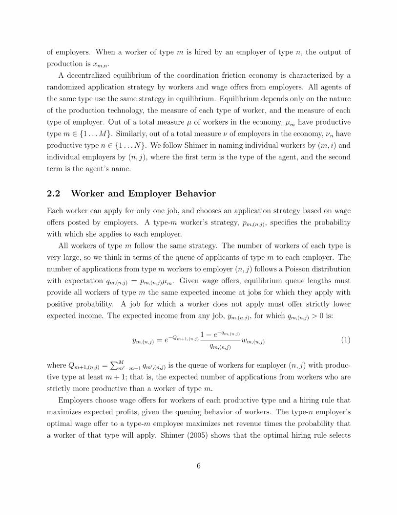
2.2 Worker and Employer Behavior

Each worker can apply for only one job, and chooses an application strategy based on wage

offers posted by employers. A type-m worker’s strategy, pm,(n,j), specifies the probability

with which she applies to each employer.

All workers of type m follow the same strategy. The number of workers of each type is

very large, so we think in terms of the queue of applicants of type m to each employer. The

number of applications from type m workers to employer (n, j) follows a Poisson distribution

with expectation qm,(n,j) = pm,(n,j)µm. Given wage offers, equilibrium queue lengths must

provide all workers of type m the same expected income at jobs for which they apply with

positive probability. A job for which a worker does not apply must offer strictly lower

expected income. The expected income from any job, ym,(n,j), for which qm,(n,j) > 0 is:

ym,(n,j) = e−Qm+1,(n,j)1− e−qm,(n,j)

qm,(n,j)wm,(n,j) (1)

where Qm+1,(n,j) =∑M

m′=m+1 qm′,(n,j) is the queue of workers for employer (n, j) with produc-

tive type at least m+ 1; that is, the expected number of applications from workers who are

strictly more productive than a worker of type m.

Employers choose wage offers for workers of each productive type and a hiring rule that

maximizes expected profits, given the queuing behavior of workers. The type-n employer’s

optimal wage offer to a type-m employee maximizes net revenue times the probability that

a worker of that type will apply. Shimer (2005) shows that the optimal hiring rule selects

6

the applicant with highest ability. When following this rule, the expected profit of employer

(n, j) is given by

π(n,j) =M∑m=1

e−Qm+1,(n,j)[1− e−qm,(n,j)

] [xm,n − wm,(n,j)

]. (2)

2.3 Search Equilibrium

Definition 1 (Shimer 2005) A Competitive Search Equilibrium consists of wage offers, w, and

queue lengths, q, chosen such that employer’s expected profits (2) are maximized, worker’s

expected incomes are given by (1), and the expected number of applications from type m

workers does not exceed the total measure of such workers, µm:

µm ≥N∑n=1

∫ νn

0

qm,(n,j)dj =N∑n=1

qm,nνn. (3)

The equality of the second and third terms in (3) arises because workers of the same type

choose the same application strategy and firms of the same type make the same wage offers.

Shimer proves the competitive equilibrium exists and is unique. He also shows the equi-

librium queue lengths, qm,n, are those that would be chosen by a social planner seeking to

maximize expected output, and who also faces coordination frictions. Letting υm be the

multiplier on the resource constraint given by equation (3), the Lagrangian for the social

planning problem is

L (q, υ) =M∑m=1

N∑n=1

νn[e−Qm+1,n

(1− e−qm,n

)xm,n

]+ υm

(µm −

N∑n=1

qm,nνn

). (4)

Given the optimal queue lengths, and the requirement that workers’ expected incomes

satisfy (1), the equilibrium wages are:

wm,n =qm,ne

−qm,n

1− e−qm,n

[xm,n −

m−1∑m′=1

e−Qm′+1,n(1− e−qm′,n

)xm′,n

]. (5)

2.4 Empirical Implications

Equations (4) and (5) provide all the information required for estimation. Given the pro-

duction technology, xm,n, and the measure of each type of employer and worker, equilibrium

7

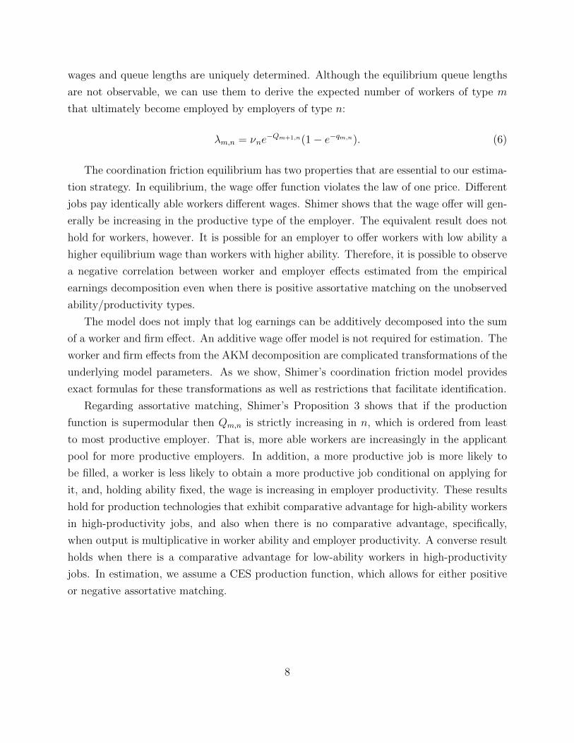
wages and queue lengths are uniquely determined. Although the equilibrium queue lengths

are not observable, we can use them to derive the expected number of workers of type m

that ultimately become employed by employers of type n:

λm,n = νne−Qm+1,n(1− e−qm,n). (6)

The coordination friction equilibrium has two properties that are essential to our estima-

tion strategy. In equilibrium, the wage offer function violates the law of one price. Different

jobs pay identically able workers different wages. Shimer shows that the wage offer will gen-

erally be increasing in the productive type of the employer. The equivalent result does not

hold for workers, however. It is possible for an employer to offer workers with low ability a

higher equilibrium wage than workers with higher ability. Therefore, it is possible to observe

a negative correlation between worker and employer effects estimated from the empirical

earnings decomposition even when there is positive assortative matching on the unobserved

ability/productivity types.

The model does not imply that log earnings can be additively decomposed into the sum

of a worker and firm effect. An additive wage offer model is not required for estimation. The

worker and firm effects from the AKM decomposition are complicated transformations of the

underlying model parameters. As we show, Shimer’s coordination friction model provides

exact formulas for these transformations as well as restrictions that facilitate identification.

Regarding assortative matching, Shimer’s Proposition 3 shows that if the production

function is supermodular then Qm,n is strictly increasing in n, which is ordered from least

to most productive employer. That is, more able workers are increasingly in the applicant

pool for more productive employers. In addition, a more productive job is more likely to

be filled, a worker is less likely to obtain a more productive job conditional on applying for

it, and, holding ability fixed, the wage is increasing in employer productivity. These results

hold for production technologies that exhibit comparative advantage for high-ability workers

in high-productivity jobs, and also when there is no comparative advantage, specifically,

when output is multiplicative in worker ability and employer productivity. A converse result

holds when there is a comparative advantage for low-ability workers in high-productivity

jobs. In estimation, we assume a CES production function, which allows for either positive

or negative assortative matching.

8

3 Empirical and Theoretical Earnings Decomposition

The novelty in our empirical approach is to formally relate the equilibrium quantities from the

structural assignment model to heterogeneity components from the statistical decomposition

of earnings associated with workers and employers. The worker and employer effects from

the earnings decomposition are complicated transformations of the equilibrium quantities.

So is the correlation between worker and employer effects across realized matches, as well as

other moments of their observed joint distribution. We explicitly derive the map between

structural equilibrium quantities and empirical moments used for estimation.

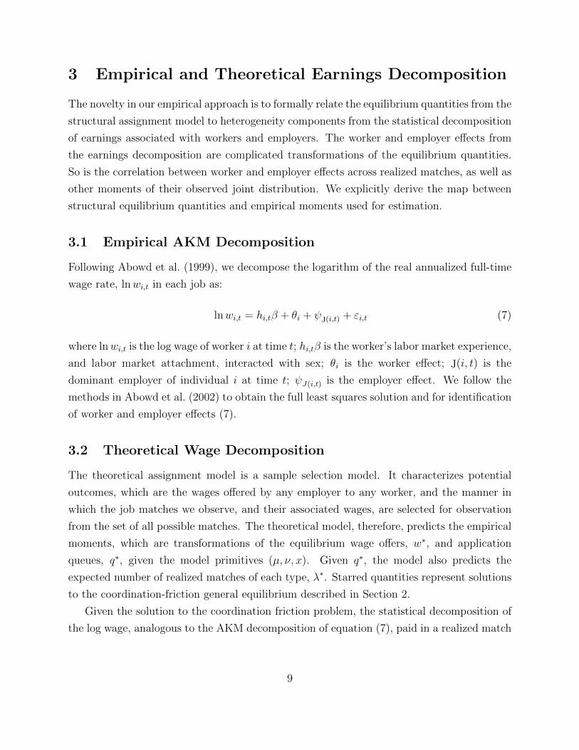
3.1 Empirical AKM Decomposition

Following Abowd et al. (1999), we decompose the logarithm of the real annualized full-time

wage rate, lnwi,t in each job as:

lnwi,t = hi,tβ + θi + ψJ(i,t) + εi,t (7)

where lnwi,t is the log wage of worker i at time t; hi,tβ is the worker’s labor market experience,

and labor market attachment, interacted with sex; θi is the worker effect; J(i, t) is the

dominant employer of individual i at time t; ψJ(i,t) is the employer effect. We follow the

methods in Abowd et al. (2002) to obtain the full least squares solution and for identification

of worker and employer effects (7).

3.2 Theoretical Wage Decomposition

The theoretical assignment model is a sample selection model. It characterizes potential

outcomes, which are the wages offered by any employer to any worker, and the manner in

which the job matches we observe, and their associated wages, are selected for observation

from the set of all possible matches. The theoretical model, therefore, predicts the empirical

moments, which are transformations of the equilibrium wage offers, w∗, and application

queues, q∗, given the model primitives (µ, ν, x). Given q∗, the model also predicts the

expected number of realized matches of each type, λ∗. Starred quantities represent solutions

to the coordination-friction general equilibrium described in Section 2.

Given the solution to the coordination friction problem, the statistical decomposition of

the log wage, analogous to the AKM decomposition of equation (7), paid in a realized match

9

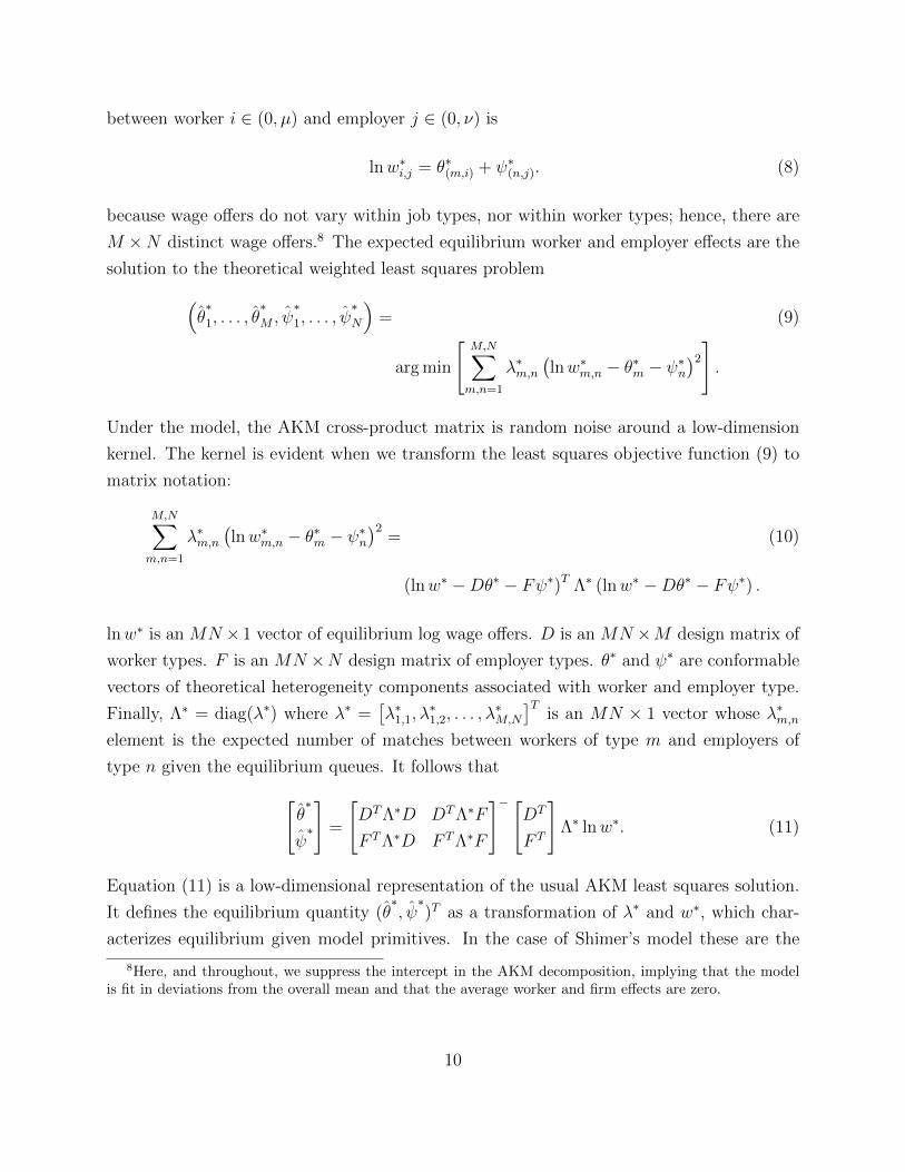
between worker i ∈ (0, µ) and employer j ∈ (0, ν) is

lnw∗i,j = θ∗(m,i) + ψ∗(n,j). (8)

because wage offers do not vary within job types, nor within worker types; hence, there are

M ×N distinct wage offers.8 The expected equilibrium worker and employer effects are the

solution to the theoretical weighted least squares problem(θ∗1, . . . , θ

∗M , ψ

∗1, . . . , ψ

∗N

)= (9)

arg min

[M,N∑m,n=1

λ∗m,n(lnw∗m,n − θ∗m − ψ∗n

)2

].

Under the model, the AKM cross-product matrix is random noise around a low-dimension

kernel. The kernel is evident when we transform the least squares objective function (9) to

matrix notation:

M,N∑m,n=1

λ∗m,n(lnw∗m,n − θ∗m − ψ∗n

)2= (10)

(lnw∗ −Dθ∗ − Fψ∗)T Λ∗ (lnw∗ −Dθ∗ − Fψ∗) .

lnw∗ is an MN × 1 vector of equilibrium log wage offers. D is an MN ×M design matrix of

worker types. F is an MN ×N design matrix of employer types. θ∗ and ψ∗ are conformable

vectors of theoretical heterogeneity components associated with worker and employer type.

Finally, Λ∗ = diag(λ∗) where λ∗ =[λ∗1,1, λ

∗1,2, . . . , λ

∗M,N

]Tis an MN × 1 vector whose λ∗m,n

element is the expected number of matches between workers of type m and employers of

type n given the equilibrium queues. It follows that[θ∗

ψ∗

]=

[DTΛ∗D DTΛ∗F

F TΛ∗D F TΛ∗F

]− [DT

F T

]Λ∗ lnw∗. (11)

Equation (11) is a low-dimensional representation of the usual AKM least squares solution.

It defines the equilibrium quantity (θ∗, ψ∗)T as a transformation of λ∗ and w∗, which char-

acterizes equilibrium given model primitives. In the case of Shimer’s model these are the

8Here, and throughout, we suppress the intercept in the AKM decomposition, implying that the modelis fit in deviations from the overall mean and that the average worker and firm effects are zero.

10

distributions of workers and employers across productive types and the production technol-

ogy: (µ, ν, x). Our empirical strategy therefore requires a model that predicts equilibrium

matching sets and wage offers, but does not specifically require Shimer’s coordination friction

model.9

Identification of(θ∗, ψ∗)

The model worker and employer wage effects,(θ∗, ψ∗)

, are identified when the cross product

matrix in equation (11) has full rank, implying that the g-inverse can be replaced by a regular

inverse. This requires Λ∗ to have full rank as well as standard identifying restrictions on D

and F .

For consistency with the empirical procedure applied to the LEHD data, we implement

identification in the theoretical decomposition by setting the mean overall worker and em-

ployer effects to zero across matches. We use the notation (θ∗, ψ∗) to refer to the components

of earnings derived from (11). For estimation, we match moments of the joint distribution

of (θ∗, ψ∗) across matches predicted under the model to their empirical counterparts.

4 Data and Estimating Equations

We use estimates of worker and employer effects from the AKM decomposition (7) applied

to LEHD data. For every employment match, in every year, we record the estimated worker

effect, θi, and estimated employer effect, ψJ(i,t), along with the NAICS sector to which the

employer belongs. The result is a dataset, (θi, ψJ(i,t), sJ(i,t))i,t, where sJ(i,t) ∈ 1, . . . , 20records the sector.

Within each sector, s, we estimate eight empirical moments:10

• g(s)1 = E(θ|s), the mean worker effect in sector s;

• g(s)2 = E(ψ|s), the mean employer effect in s;

• g(s)3 = V ar(θ|s), the variance of worker effects in s;

• g(s)4 = Cov(θ, ψ|s), the covariance between worker and employer effects in s;

9Appendix C presents the case with a continuum of employer types.10We estimate the sampling covariance of g

(s)1 , . . . , g

(s)6 , using 1, 000 bootstrap samples from the raw

microdata. The estimated sampling covariance matrix is included with the data archive.

11

• g(s)5 = V ar(ψ|s), the variance of employer effects in s;

• g(s)6 = Z(s), the share of matches in sector s;

• g(s)7 = R(s), the rate of vacant job openings in s;

• g(s)8 = Y (s), value-added per worker in s.

4.1 Data Sources

To compute moments g(s)1 , . . . , g

(s)6 , we use matched employer-employee data from the Lon-

gitudinal Employer-Household Dynamics (LEHD) Program of the U.S. Census Bureau. The

LEHD Program uses administrative data from state Unemployment Insurance wage records

and ES-202/QCEW establishment reports that cover approximately 98 percent of all non-

farm U.S. employment. Our estimation sample is based on a snapshot of the LEHD data

infrastructure that includes information from twenty-eight states collected between 1990 and

2004.11 Appendix B provides a detailed description of the LEHD data.

Data on sectoral vacancy rates, g(s)7 = R(s), are from the Job Openings and Labor

Turnover Survey (JOLTS). The vacancy rates for sector sj reported in JOLTS is the em-

pirical average across firms of the number of vacancies divided by the sum of vacancies and

employment. This statistic has an interpretation as the probability that a job opening in

sector s is left vacant. Using the monthly JOLTS data disaggregated by sector for the years

2001-2003, we compute g(s)7 as the simple average of the monthly observations for sector s.

To measure the sampling variance of g(s)7 , we combined the median cross-sectional standard

error (squared) of the job opening rate for each sector with that rate’s time-series variation.12

We measure sectoral productivity, g(s)8 , using data on value-added per worker from the

Bureau of Economic Analysis (BEA) Annual Industry Accounts.13 For each year between

1990-2003 (corresponding to our years of LEHD data), we take the BEA report of total

value-added by NAICS sector in millions of chained 2005 dollars and deflate by reported

11Only the first quarter of 2004 is available in this snapshot. The annualized real wage rate is, therefore,only available for the years 1990-2003.

12The sectoral classification for the public-use JOLTS data does not quite conform to the NAICS 2002major sectors. We use a custom crosswalk that maps JOLTS sectors, which are generally more coarse, ontoNAICS 2002. The details of the crosswalk are available upon request. We obtained median standard errorsfor 2013 by industry from JOLTSInfo@bls.gov.

13The BEA data are from the files GDPbyInd VA NAICS 1998-2011.xlsx andGDPbyInd VA NAICS 1947-1997.xls, retrieved from http://www.bea.gov/industry/gdpbyind data.htm

on 2013-03-20.

12

employment in that sector. This yields a measure of value-added per worker for each year.

We compute the moment used in estimation, g(s)8 , and its sampling variance, s

(s)8 , as the

simple average and variance across the annual observations for sector k.

4.2 Data Summary and Data Availability

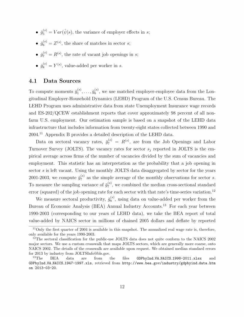
Table 1 reports the empirical moments used in estimation. These moments are publicly

Table 1: Empirical Moments by NAICS Major Sector

Cov Emp. Vac. Val. CorrSector E(θ) E(ψ) Var(θ) (θ, ψ) Var(ψ) Share Rate Add. (θ, ψ)

Agr. and related -0.158 -0.194 0.533 0.016 0.188 0.015 0.016 0.066 0.052Administration -0.084 -0.112 0.483 0.053 0.198 0.064 0.039 0.037 0.170Other Services -0.036 -0.044 0.451 -0.042 0.234 0.031 0.032 0.051 -0.129Manufacturing -0.007 0.292 0.293 0.007 0.079 0.164 0.016 0.069 0.047Accommodation 0.010 -0.358 0.468 -0.009 0.099 0.055 0.038 0.031 -0.044Health 0.034 0.080 0.422 0.008 0.082 0.099 0.046 0.057 0.041Utilities 0.035 0.535 0.210 -0.019 0.092 0.008 0.021 0.316 -0.135Transportation 0.036 0.142 0.334 -0.014 0.113 0.037 0.021 0.068 -0.070Govt. Services 0.039 0.121 0.318 -0.015 0.107 0.043 0.019 0.065 -0.083Mining 0.040 0.486 0.334 0.005 0.088 0.005 0.016 0.461 0.027Construction 0.040 0.204 0.334 -0.005 0.106 0.067 0.019 0.097 -0.027Real Estate 0.041 0.071 0.436 -0.012 0.160 0.016 0.023 0.652 -0.043Retail 0.076 -0.119 0.391 -0.007 0.106 0.111 0.024 0.044 -0.036Arts 0.100 -0.225 0.569 -0.004 0.248 0.013 0.031 0.063 -0.012Wholesale 0.124 0.232 0.361 0.002 0.118 0.052 0.021 0.086 0.010Information 0.166 0.287 0.462 0.001 0.234 0.030 0.028 0.113 0.030Finance 0.168 0.275 0.358 0.005 0.088 0.049 0.032 0.129 0.026Management 0.187 0.348 0.379 0.014 0.087 0.007 0.039 0.121 0.078Professions 0.221 0.317 0.408 0.017 0.214 0.058 0.039 0.103 0.057Education 0.236 -0.175 0.455 -0.027 0.087 0.076 0.019 0.047 -0.137

SOURCE - The moments in θ and ψ are based on authors’ calculations of person- and firm-specificcomponents of log earnings. These, and the employment shares, are estimated from LEHD databetween 1990-2003. Data on value-added per worker by sector are as reported in the Bureau ofEconomic Analysis (BEA) Annual Industry Accounts.

available in more detail than we report here.14 It is not trivial to provide these data while

maintaining the confidentiality of respondents providing the underlying microdata. The

Census Bureau is not generally willing to release detailed descriptive statistics apart from

the normally published data products. The data we have made available are protected by a

distribution-preserving noise-infusion procedure. For complete details of the noise infusion

14 The moments of worker and employer effects are available disaggregated by firm size within sectors.Bootstrapped estimates of the sampling covariances are also available. The data are permanently archivedat http://digitalcommons.ilr.cornell.edu/ldi/21.

13

procedure and the way it preserves analytical validity, see Abowd, Gittings, McKinney,

Stephens, Vilhuber and Woodcock (2012).

5 Parameterization and Estimation Details

We fit the coordination friction model to 159 unrestricted moments.15 The model predicts

the components of the AKM decomposition, (θ∗, ψ∗), their joint distribution in realized

matches within and across sectors, the sectoral distribution of employment, sectoral output

per worker, and sectoral vacancies. This is sufficient information to compute theoretical

analogues to the empirical moments. Formulas for the estimating equations in terms of

model primitives and equilibrium quantities are fully specified in Appendix E.

5.1 Parameterization of the Coordination Friction Economy

We fit a vector, ζ = (µ, ν, h, χ, ε, φ, β, ρ, ς), of 52 structural parameters. The parameter µm

measures the share of workers of type m. We assume M = 5 types of worker and impose,

without loss of generality, that∑

m′ µm′ = 1, leaving four free parameters. Each type m

worker is endowed with productivity, hm ∈ (0, 1).16 In estimation, we require that the

worker productivity distribution have mass at h2 = 0.25 and h4 = 0.75. We then estimate

h1, h3, and h5 as free parameters on [0, 0.25), (0.25, 0.75), and (0.75, 1], respectively.

The model assumes a single dimension of productive heterogeneity across employers. We

now specify how productivity varies across and within sector. We model 20 sectors that each

offer 3 latent job types. There are thus N = 60 job types distinguished by productivity. The

index n of the job is (s, `), where s = 1, ..., 20 indicates the sector and ` = 1, ..., 3 indicates

the productive job type for that sector. The parameter νn = νs,` is the measure of jobs of

type n. The total number of openings in each sector is a free parameter, and we assume

openings are uniformly distributed across the three latent job types.

Employer productivity, kn = ks,` ∈ (0, 1), varies by sector and the latent job type. We

define kn as

kn ≡ ks,` = φχ(s) + (1− φ) εkj. (12)

where kj ∈ 0.1, 0.5, 0.9 is a grid over latent levels of employer productivity. Productivity

15Because the employment shares sum to one, we delete one sector share–NAICS government (92).16We impose that worker productivity is strictly increasing across types: hm′ > hm whenever m′ > m.

This restriction avoids solutions that simply relabel the worker types.

14

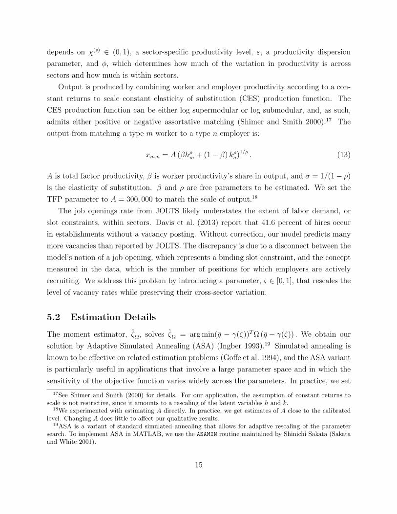
depends on χ(s) ∈ (0, 1), a sector-specific productivity level, ε, a productivity dispersion

parameter, and φ, which determines how much of the variation in productivity is across

sectors and how much is within sectors.

Output is produced by combining worker and employer productivity according to a con-

stant returns to scale constant elasticity of substitution (CES) production function. The

CES production function can be either log supermodular or log submodular, and, as such,

admits either positive or negative assortative matching (Shimer and Smith 2000).17 The

output from matching a type m worker to a type n employer is:

xm,n = A (βhρm + (1− β) kρn)1/ρ . (13)

A is total factor productivity, β is worker productivity’s share in output, and σ = 1/(1− ρ)

is the elasticity of substitution. β and ρ are free parameters to be estimated. We set the

TFP parameter to A = 300, 000 to match the scale of output.18

The job openings rate from JOLTS likely understates the extent of labor demand, or

slot constraints, within sectors. Davis et al. (2013) report that 41.6 percent of hires occur

in establishments without a vacancy posting. Without correction, our model predicts many

more vacancies than reported by JOLTS. The discrepancy is due to a disconnect between the

model’s notion of a job opening, which represents a binding slot constraint, and the concept

measured in the data, which is the number of positions for which employers are actively

recruiting. We address this problem by introducing a parameter, ς ∈ [0, 1], that rescales the

level of vacancy rates while preserving their cross-sector variation.

5.2 Estimation Details

The moment estimator, ζΩ, solves ζΩ = arg min(g − γ(ζ))TΩ (g − γ(ζ)) . We obtain our

solution by Adaptive Simulated Annealing (ASA) (Ingber 1993).19 Simulated annealing is

known to be effective on related estimation problems (Goffe et al. 1994), and the ASA variant

is particularly useful in applications that involve a large parameter space and in which the

sensitivity of the objective function varies widely across the parameters. In practice, we set

17See Shimer and Smith (2000) for details. For our application, the assumption of constant returns toscale is not restrictive, since it amounts to a rescaling of the latent variables h and k.

18We experimented with estimating A directly. In practice, we get estimates of A close to the calibratedlevel. Changing A does little to affect our qualitative results.

19ASA is a variant of standard simulated annealing that allows for adaptive rescaling of the parametersearch. To implement ASA in MATLAB, we use the ASAMIN routine maintained by Shinichi Sakata (Sakataand White 2001).

15

Ω = I, the identity matrix.

At each iteration in the algorithm, ASA proposes a vector of structural parameters, ζ.

At ζ, we solve the planner’s problem in the coordination-friction economy in equation (4)

numerically. 20 Equilibrium queue lengths in the decentralized economy are identical to those

the planner chooses, and we obtain the equilibrium wage offers by application of equation

(5). With the matching set and wage offers in hand, we calculate the theoretical moments

as in Section 3.2. 21

5.3 Identification

5.3.1 Identification of Equilibrium Wages and Matching Sets

The data generating process identifies the joint distribution of observed wages and error

components from the linear decomposition of log wages into person and employer-specific

components. From equation (11), the identified quantities are the wage components associ-

ated with each worker and employer heterogeneity class,(Dθ∗, F ψ

∗). The data also identify

their joint distribution with observed (log) wages across matches(Λ∗ lnw∗,Λ∗Dθ

∗,Λ∗Fψ

∗). (14)

Our identification argument relies on discretizing the worker and employer types across

matches. It follows that the expected equilibrium matching set, Λ∗, is identified by solving

for (Λ∗ − I) in

Λ∗Dθ∗−Dθ

∗= (Λ∗ − I)Dθ

∗,

which is feasible since (Λ∗ − I) is diagonal. As long as Λ∗ is full rank, it is then possible to

recover the vector of equilibrium log wage offers lnw∗, from the observed wage distribution.

5.3.2 Identification of Equilibrium Queues and Match Output

Even though we observe which workers earn the most and which firms pay the most, we

cannot rank the classes by ability or productivity without additional model information.

Shimer’s model implies that expected income is identical across jobs for workers of a given

ability type. Furthermore, expected income is equal to the expected marginal product.

20The planner’s problem is convex, so a global minimum is guaranteed to exist.21Once the simulated annealing procedure converges to an estimate, ζA, we estimate its covariance matrix

as: (FTΩF )−1FTΩSΩF (FTΩF )−1 where F = F (ζ) = ∂f(ζ)∂ζ and S is the covariance matrix of g.

16

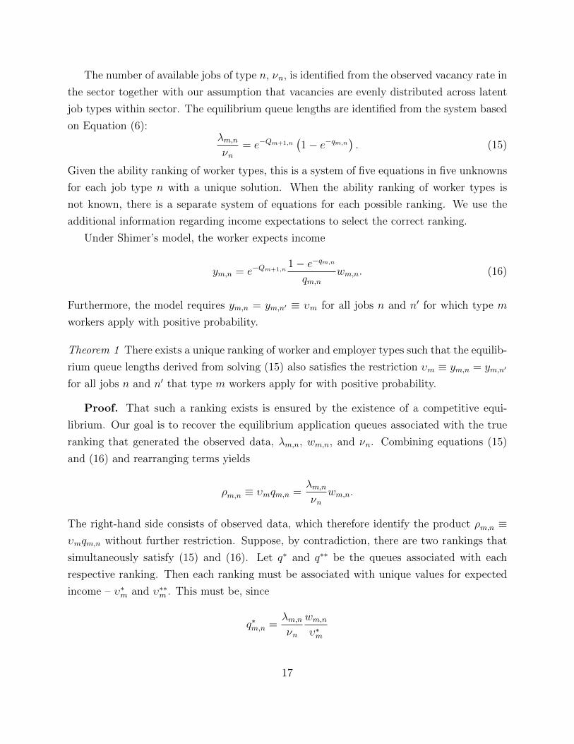
The number of available jobs of type n, νn, is identified from the observed vacancy rate in

the sector together with our assumption that vacancies are evenly distributed across latent

job types within sector. The equilibrium queue lengths are identified from the system based

on Equation (6):λm,nνn

= e−Qm+1,n(1− e−qm,n

). (15)

Given the ability ranking of worker types, this is a system of five equations in five unknowns

for each job type n with a unique solution. When the ability ranking of worker types is

not known, there is a separate system of equations for each possible ranking. We use the

additional information regarding income expectations to select the correct ranking.

Under Shimer’s model, the worker expects income

ym,n = e−Qm+1,n1− e−qm,n

qm,nwm,n. (16)

Furthermore, the model requires ym,n = ym,n′ ≡ υm for all jobs n and n′ for which type m

workers apply with positive probability.

Theorem 1 There exists a unique ranking of worker and employer types such that the equilib-

rium queue lengths derived from solving (15) also satisfies the restriction υm ≡ ym,n = ym,n′

for all jobs n and n′ that type m workers apply for with positive probability.

Proof. That such a ranking exists is ensured by the existence of a competitive equi-

librium. Our goal is to recover the equilibrium application queues associated with the true

ranking that generated the observed data, λm,n, wm,n, and νn. Combining equations (15)

and (16) and rearranging terms yields

ρm,n ≡ υmqm,n =λm,nνn

wm,n.

The right-hand side consists of observed data, which therefore identify the product ρm,n ≡υmqm,n without further restriction. Suppose, by contradiction, there are two rankings that

simultaneously satisfy (15) and (16). Let q∗ and q∗∗ be the queues associated with each

respective ranking. Then each ranking must be associated with unique values for expected

income – υ∗m and υ∗∗m . This must be, since

q∗m,n =λm,nνn

wm,nυ∗m

17

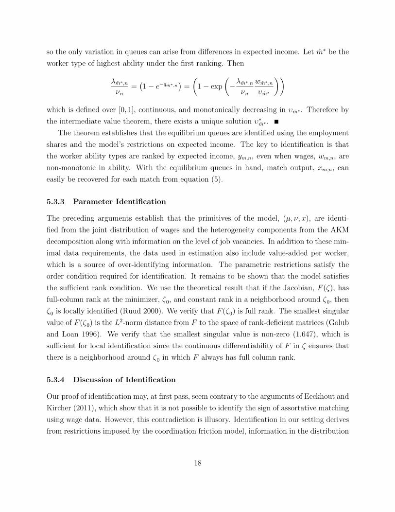
so the only variation in queues can arise from differences in expected income. Let m∗ be the

worker type of highest ability under the first ranking. Then

λm∗,nνn

=(1− e−qm∗,n

)=

(1− exp

(−λm

∗,n

νn

wm∗,nυm∗

))which is defined over [0, 1], continuous, and monotonically decreasing in υm∗ . Therefore by

the intermediate value theorem, there exists a unique solution υ∗m∗ .

The theorem establishes that the equilibrium queues are identified using the employment

shares and the model’s restrictions on expected income. The key to identification is that

the worker ability types are ranked by expected income, ym,n, even when wages, wm,n, are

non-monotonic in ability. With the equilibrium queues in hand, match output, xm,n, can

easily be recovered for each match from equation (5).

5.3.3 Parameter Identification

The preceding arguments establish that the primitives of the model, (µ, ν, x), are identi-

fied from the joint distribution of wages and the heterogeneity components from the AKM

decomposition along with information on the level of job vacancies. In addition to these min-

imal data requirements, the data used in estimation also include value-added per worker,

which is a source of over-identifying information. The parametric restrictions satisfy the

order condition required for identification. It remains to be shown that the model satisfies

the sufficient rank condition. We use the theoretical result that if the Jacobian, F (ζ), has

full-column rank at the minimizer, ζ0, and constant rank in a neighborhood around ζ0, then

ζ0 is locally identified (Ruud 2000). We verify that F (ζ0) is full rank. The smallest singular

value of F (ζ0) is the L2-norm distance from F to the space of rank-deficient matrices (Golub

and Loan 1996). We verify that the smallest singular value is non-zero (1.647), which is

sufficient for local identification since the continuous differentiability of F in ζ ensures that

there is a neighborhood around ζ0 in which F always has full column rank.

5.3.4 Discussion of Identification

Our proof of identification may, at first pass, seem contrary to the arguments of Eeckhout and

Kircher (2011), which show that it is not possible to identify the sign of assortative matching

using wage data. However, this contradiction is illusory. Identification in our setting derives

from restrictions imposed by the coordination friction model, information in the distribution

18

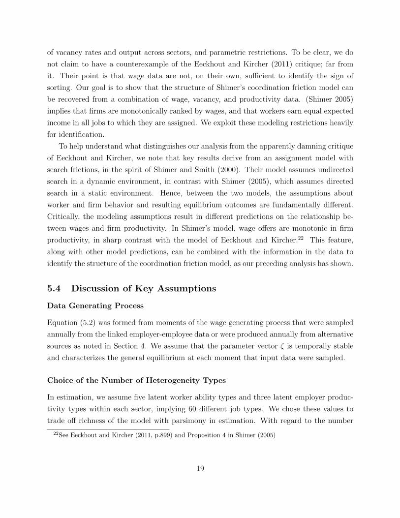
of vacancy rates and output across sectors, and parametric restrictions. To be clear, we do

not claim to have a counterexample of the Eeckhout and Kircher (2011) critique; far from

it. Their point is that wage data are not, on their own, sufficient to identify the sign of

sorting. Our goal is to show that the structure of Shimer’s coordination friction model can

be recovered from a combination of wage, vacancy, and productivity data. (Shimer 2005)

implies that firms are monotonically ranked by wages, and that workers earn equal expected

income in all jobs to which they are assigned. We exploit these modeling restrictions heavily

for identification.

To help understand what distinguishes our analysis from the apparently damning critique

of Eeckhout and Kircher, we note that key results derive from an assignment model with

search frictions, in the spirit of Shimer and Smith (2000). Their model assumes undirected

search in a dynamic environment, in contrast with Shimer (2005), which assumes directed

search in a static environment. Hence, between the two models, the assumptions about

worker and firm behavior and resulting equilibrium outcomes are fundamentally different.

Critically, the modeling assumptions result in different predictions on the relationship be-

tween wages and firm productivity. In Shimer’s model, wage offers are monotonic in firm

productivity, in sharp contrast with the model of Eeckhout and Kircher.22 This feature,

along with other model predictions, can be combined with the information in the data to

identify the structure of the coordination friction model, as our preceding analysis has shown.

5.4 Discussion of Key Assumptions

Data Generating Process

Equation (5.2) was formed from moments of the wage generating process that were sampled

annually from the linked employer-employee data or were produced annually from alternative

sources as noted in Section 4. We assume that the parameter vector ζ is temporally stable

and characterizes the general equilibrium at each moment that input data were sampled.

Choice of the Number of Heterogeneity Types

In estimation, we assume five latent worker ability types and three latent employer produc-

tivity types within each sector, implying 60 different job types. We chose these values to

trade off richness of the model with parsimony in estimation. With regard to the number

22See Eeckhout and Kircher (2011, p.899) and Proposition 4 in Shimer (2005)

19

of worker types, it is necessary to allow for more than two in order for an inversion of the

relationship between unobserved ability and wages to be estimable in the data. Our choice

of five worker types allows such an inversion to unfold at different points in the ability distri-

bution. Adding more latent employer and worker types does not improve the model enough

to overcome any reasonable penalty for the additional free parameters.

6 Results

Our estimates indicate strong positive assortative matching in the assignment of workers

to employers across sectors. The AKM worker and employer effects conceal assortative

matching because of non-monotonicity in the estimated worker wage effects with respect to

worker ability. In combination with the selection of realized matches, this non-monotonicity

hides the true correlation between unobserved worker ability and employer productivity.23

6.1 Model Primitives

We first report the estimated model primitives: the distribution of workers across latent

ability types, the distribution of job openings across sectors and latent productivity types,

and the production function that characterizes match output.

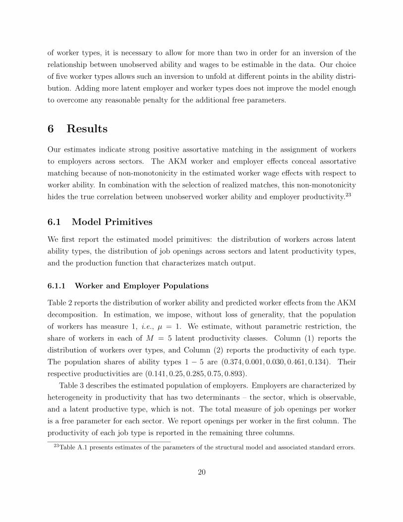
6.1.1 Worker and Employer Populations

Table 2 reports the distribution of worker ability and predicted worker effects from the AKM

decomposition. In estimation, we impose, without loss of generality, that the population

of workers has measure 1, i.e., µ = 1. We estimate, without parametric restriction, the

share of workers in each of M = 5 latent productivity classes. Column (1) reports the

distribution of workers over types, and Column (2) reports the productivity of each type.

The population shares of ability types 1 − 5 are (0.374, 0.001, 0.030, 0.461, 0.134). Their

respective productivities are (0.141, 0.25, 0.285, 0.75, 0.893).

Table 3 describes the estimated population of employers. Employers are characterized by

heterogeneity in productivity that has two determinants – the sector, which is observable,

and a latent productive type, which is not. The total measure of job openings per worker

is a free parameter for each sector. We report openings per worker in the first column. The

productivity of each job type is reported in the remaining three columns.

23Table A.1 presents estimates of the parameters of the structural model and associated standard errors.

20

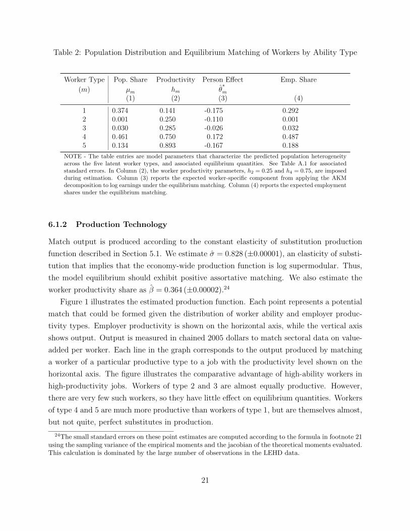
Table 2: Population Distribution and Equilibrium Matching of Workers by Ability Type

Worker Type Pop. Share Productivity Person Effect Emp. Share

(m) µm hm θ∗m

(1) (2) (3) (4)

1 0.374 0.141 -0.175 0.2922 0.001 0.250 -0.110 0.0013 0.030 0.285 -0.026 0.0324 0.461 0.750 0.172 0.4875 0.134 0.893 -0.167 0.188

NOTE - The table entries are model parameters that characterize the predicted population heterogeneityacross the five latent worker types, and associated equilibrium quantities. See Table A.1 for associatedstandard errors. In Column (2), the worker productivity parameters, h2 = 0.25 and h4 = 0.75, are imposedduring estimation. Column (3) reports the expected worker-specific component from applying the AKMdecomposition to log earnings under the equilibrium matching. Column (4) reports the expected employmentshares under the equilibrium matching.

6.1.2 Production Technology

Match output is produced according to the constant elasticity of substitution production

function described in Section 5.1. We estimate σ = 0.828 (±0.00001), an elasticity of substi-

tution that implies that the economy-wide production function is log supermodular. Thus,

the model equilibrium should exhibit positive assortative matching. We also estimate the

worker productivity share as β = 0.364 (±0.00002).24

Figure 1 illustrates the estimated production function. Each point represents a potential

match that could be formed given the distribution of worker ability and employer produc-

tivity types. Employer productivity is shown on the horizontal axis, while the vertical axis

shows output. Output is measured in chained 2005 dollars to match sectoral data on value-

added per worker. Each line in the graph corresponds to the output produced by matching

a worker of a particular productive type to a job with the productivity level shown on the

horizontal axis. The figure illustrates the comparative advantage of high-ability workers in

high-productivity jobs. Workers of type 2 and 3 are almost equally productive. However,

there are very few such workers, so they have little effect on equilibrium quantities. Workers

of type 4 and 5 are much more productive than workers of type 1, but are themselves almost,

but not quite, perfect substitutes in production.

24The small standard errors on these point estimates are computed according to the formula in footnote 21using the sampling variance of the empirical moments and the jacobian of the theoretical moments evaluated.This calculation is dominated by the large number of observations in the LEHD data.

21

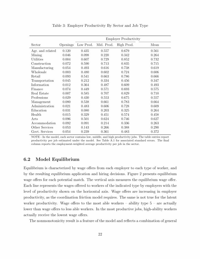
Table 3: Employer Productivity By Sector and Job Type

Employer Productivity

Sector Openings Low Prod. Mid. Prod. High Prod. Mean

Agr. and related 0.120 0.435 0.557 0.679 0.561Mining 0.046 0.098 0.220 0.342 0.264Utilities 0.004 0.607 0.729 0.852 0.732Construction 0.072 0.590 0.713 0.835 0.715Manufacturing 0.054 0.493 0.616 0.738 0.619Wholesale 0.003 0.480 0.602 0.724 0.606Retail 0.093 0.541 0.663 0.786 0.666Transportation 0.045 0.212 0.334 0.456 0.347Information 0.012 0.364 0.487 0.609 0.493Finance 0.074 0.449 0.571 0.693 0.575Real Estate 0.007 0.585 0.707 0.829 0.710Professions 0.029 0.430 0.553 0.675 0.557Management 0.080 0.538 0.661 0.783 0.664Administration 0.021 0.483 0.606 0.728 0.609Education 0.031 0.080 0.203 0.325 0.264Health 0.015 0.329 0.451 0.574 0.458Arts 0.096 0.501 0.624 0.746 0.627Accommodation 0.092 0.091 0.214 0.336 0.263Other Services 0.053 0.143 0.266 0.388 0.290Govt. Services 0.054 0.239 0.361 0.483 0.372

NOTE - In the model, each sector contains low, middle, and high productivity jobs. The table entries reportproductivity per job estimated under the model. See Table A.1 for associated standard errors. The finalcolumn reports the employment-weighted average productivity per job in the sector.

6.2 Model Equilibrium

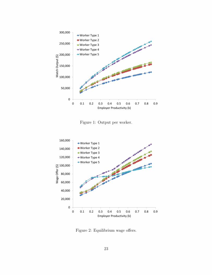
Equilibrium is characterized by wage offers from each employer to each type of worker, and

by the resulting equilibrium application and hiring decisions. Figure 2 presents equilibrium

wage offers for each potential match. The vertical axis measures the equilibrium wage offer.

Each line represents the wages offered to workers of the indicated type by employers with the

level of productivity shown on the horizontal axis. Wage offers are increasing in employer

productivity, as the coordination friction model requires. The same is not true for the latent

worker productivity. Wage offers to the most able workers – ability type 5 – are actually

lower than wage offers to less able workers. In the most productive jobs, high-ability workers

actually receive the lowest wage offers.

The nonmonotonicity result is a feature of the model and reflects a combination of general

22

0

50,000

100,000

150,000

200,000

250,000

300,000

0 0.1 0.2 0.3 0.4 0.5 0.6 0.7 0.8 0.9

Match Outpu

t ($)

Employer Productivity (k)

Worker Type 1Worker Type 2Worker Type 3Worker Type 4Worker Type 5

Figure 1: Output per worker.

0

20,000

40,000

60,000

80,000

100,000

120,000

140,000

160,000

0 0.1 0.2 0.3 0.4 0.5 0.6 0.7 0.8 0.9

Wage Offe

r ($)

Employer Productivity (k)

Worker Type 1Worker Type 2Worker Type 3Worker Type 4Worker Type 5

Figure 2: Equilibrium wage offers.

23

0.0

0.1

0.2

0.3

0.4

0.5

0.6

0.7

0.8

0.9

1.0

0 0.1 0.2 0.3 0.4 0.5 0.6 0.7 0.8 0.9

Share of Filled

Jobs

Employer Productivity (k)

Worker Type 1Worker Type 2Worker Type 3Worker Type 4Worker Type 5

Figure 3: Equilibrium matching of workers to jobs.

equilibrium factors. Unemployment risk between type 4 and type 5 workers is discontinuously

greater than the productivity difference between those types. Employers always hire a type

5 worker before a type 4 worker if both apply. The higher wage offer to type 4 reflects

a compensating differential for unemployment risk resulting from the possibility of type 5

applications. The wage offers also reflect the marginal value to the employer of attracting

another application from each type of worker. We can interpret type 4 workers’ high wage

offer as a measure of their ability to hold the employer up when the employer actually needs

their labor because there are no type 5 applicants. From the employer’s perspective, the

value of the option to hire a type 4 worker, which requires that a type 4 worker apply, is very

high in the case that no type 5 worker applies. The hold-up power of type 5 workers is very

limited for two reasons: there are relatively many other type 5 workers, and type 4 workers

are close substitutes. Thus, the marginal value to the employer of a type 5 application is

low relative to the marginal value of a type 4 application.

The equilibrium matching is characterized in Figures 3 and 4. Figure 3 shows the share

of employment in each job type for each worker type. The vertical axis measures the share

of filled jobs. Each line records the share of jobs that are filled by workers of the indicated

type. For each employer productivity level on the horizontal axis, the sum of the share of

24

0.0

0.1

0.2

0.3

0.4

0.5

0.6

0.7

0.8

0 0.1 0.2 0.3 0.4 0.5 0.6 0.7 0.8 0.9

Expe

cted

Worker P

rodu

ctivity

(h)

Employer Productivity (k)

Figure 4: Equilibrium expected worker productivity.

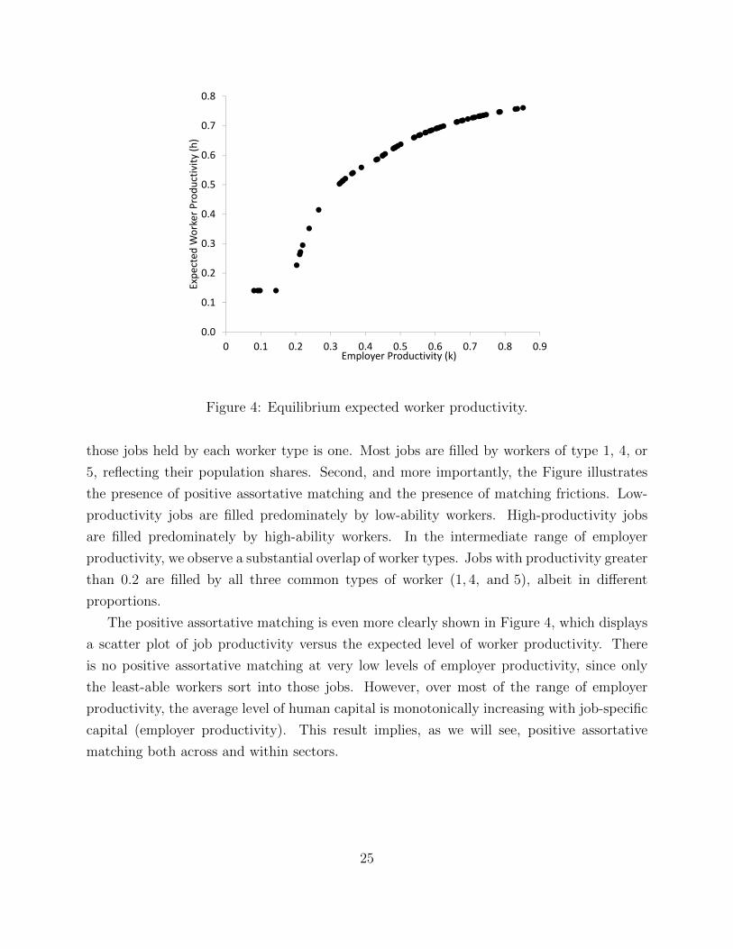
those jobs held by each worker type is one. Most jobs are filled by workers of type 1, 4, or

5, reflecting their population shares. Second, and more importantly, the Figure illustrates

the presence of positive assortative matching and the presence of matching frictions. Low-

productivity jobs are filled predominately by low-ability workers. High-productivity jobs

are filled predominately by high-ability workers. In the intermediate range of employer

productivity, we observe a substantial overlap of worker types. Jobs with productivity greater

than 0.2 are filled by all three common types of worker (1, 4, and 5), albeit in different

proportions.

The positive assortative matching is even more clearly shown in Figure 4, which displays

a scatter plot of job productivity versus the expected level of worker productivity. There

is no positive assortative matching at very low levels of employer productivity, since only

the least-able workers sort into those jobs. However, over most of the range of employer

productivity, the average level of human capital is monotonically increasing with job-specific

capital (employer productivity). This result implies, as we will see, positive assortative

matching both across and within sectors.

25

‐0.6

‐0.5

‐0.4

‐0.3

‐0.2

‐0.1

0.0

0.1

0.2

0.3

0.4

0.5

0.6

‐0.6 ‐0.5 ‐0.4 ‐0.3 ‐0.2 ‐0.1 0.0 0.1 0.2 0.3 0.4 0.5 0.6

E(ψ)

E(θ)

PredictedActual

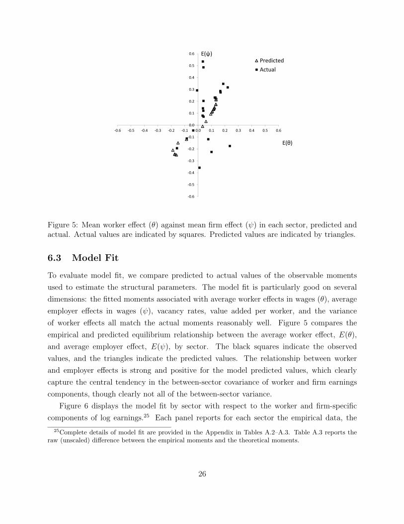
Figure 5: Mean worker effect (θ) against mean firm effect (ψ) in each sector, predicted andactual. Actual values are indicated by squares. Predicted values are indicated by triangles.

6.3 Model Fit

To evaluate model fit, we compare predicted to actual values of the observable moments

used to estimate the structural parameters. The model fit is particularly good on several

dimensions: the fitted moments associated with average worker effects in wages (θ), average

employer effects in wages (ψ), vacancy rates, value added per worker, and the variance

of worker effects all match the actual moments reasonably well. Figure 5 compares the

empirical and predicted equilibrium relationship between the average worker effect, E(θ),

and average employer effect, E(ψ), by sector. The black squares indicate the observed

values, and the triangles indicate the predicted values. The relationship between worker

and employer effects is strong and positive for the model predicted values, which clearly

capture the central tendency in the between-sector covariance of worker and firm earnings

components, though clearly not all of the between-sector variance.

Figure 6 displays the model fit by sector with respect to the worker and firm-specific

components of log earnings.25 Each panel reports for each sector the empirical data, the

25Complete details of model fit are provided in the Appendix in Tables A.2–A.3. Table A.3 reports theraw (unscaled) difference between the empirical moments and the theoretical moments.

26

-0.4

-0.2

0

0.2

0.4

0.6

0.8

Acc

omm

odat

ion

Agr

. and

rela

ted

Arts

Adm

inis

tratio

nR

etai

lO

ther

Ser

vice

sEd

ucat

ion

Tran

spor

tatio

nR

eal E

stat

eIn

form

atio

nG

ovt.

Serv

ices

Man

ufac

turin

gM

anag

emen

tC

onst

ruct

ion

Hea

lthPr

ofes

sion

sW

hole

sale

Fina

nce

Util

ities

Min

ing

E(θ) (Thr.)E(θ) (Emp.)E(h)

(a) Mean Worker Effect

-0.6

-0.4

-0.2

0

0.2

0.4

0.6

0.8

Acc

omm

odat

ion

Agr

. and

rela

ted

Arts

Adm

inis

tratio

nR

etai

lO

ther

Ser

vice

sEd

ucat

ion

Tran

spor

tatio

nR

eal E

stat

eIn

form

atio

nG

ovt.

Serv

ices

Man

ufac

turin

gM

anag

emen

tC

onst

ruct

ion

Hea

lthPr

ofes

sion

sW

hole

sale

Fina

nce

Util

ities

Min

ing

E(Ψ) (Thr.)

E(Ψ) (Emp.)

E(k)

(b) Mean Firm Effect

0

0.1

0.2

0.3

0.4

0.5

0.6

Acc

omm

odat

ion

Agr

. and

rela

ted

Arts

Adm

inis

tratio

nR

etai

lO

ther

Ser

vice

sEd

ucat

ion

Tran

spor

tatio

nR

eal E

stat

eIn

form

atio

nG

ovt.

Serv

ices

Man

ufac

turin

gM

anag

emen

tC

onst

ruct

ion

Hea

lthPr

ofes

sion

sW

hole

sale

Fina

nce

Util

ities

Min

ing

Var(θ) (Thr.)

Var(θ) (Emp.)

Var(h)

(c) Var. Worker Effect

0

0.05

0.1

0.15

0.2

0.25

0.3

Acc

omm

odat

ion

Agr

. and

rela

ted

Arts

Adm

inis

tratio

nR

etai

lO

ther

Ser

vice

sEd

ucat

ion

Tran

spor

tatio

nR

eal E

stat

eIn

form

atio

nG

ovt.

Serv

ices

Man

ufac

turin

gM

anag

emen

tC

onst

ruct

ion

Hea

lthPr

ofes

sion

sW

hole

sale

Fina

nce

Util

ities

Min

ing

Var(Ψ) (Thr.)

Var(Ψ) (Emp.)Var(k)

(d) Var. Firm Effect

Figure 6: Model Fit. Sectors sorted by predicted mean worker effect.

predicted values, and the associated latent productivity component. The sectors are sorted

by the predicted average worker effect in that sector. For instance, Figure 6a reports for

each sector the empirical average worker effect, the expected average worker effect under the

model, and the expected average worker productivity.

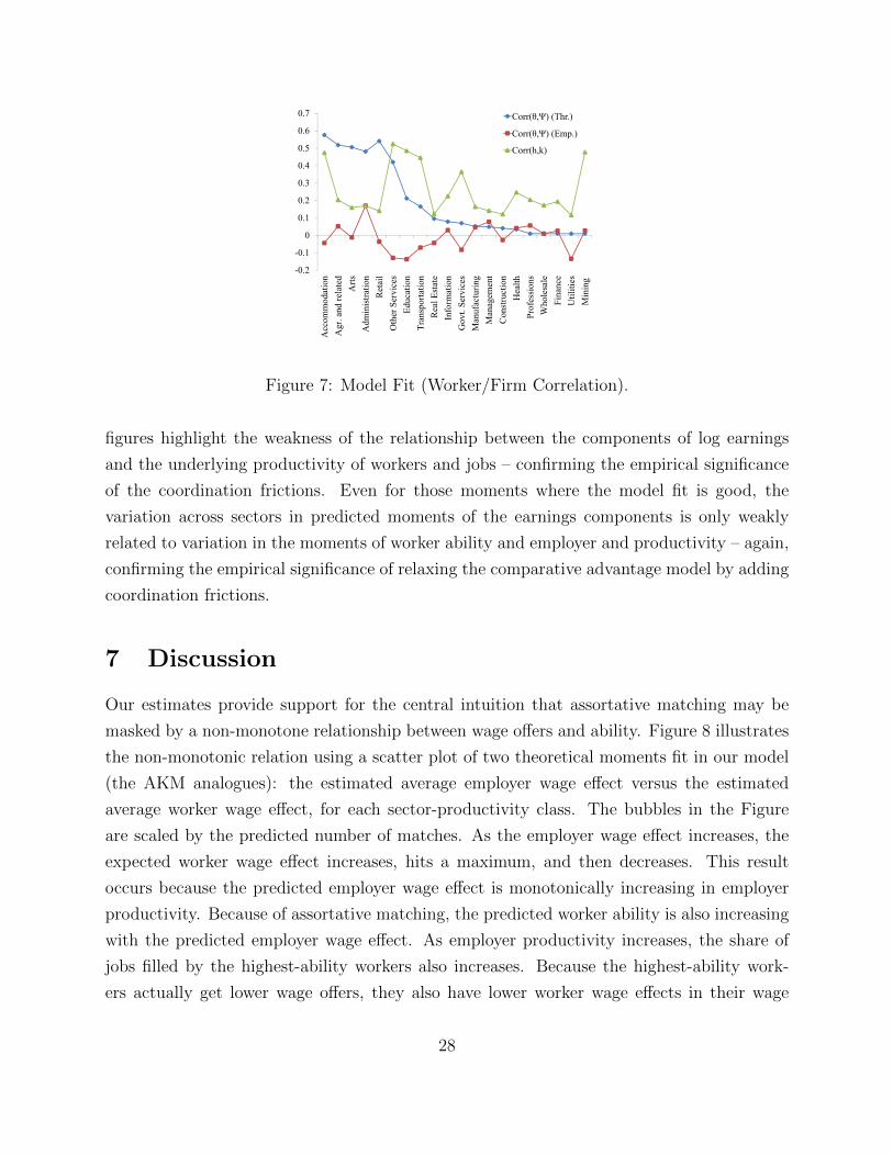
Three features of Figures 6 and 7 stand out. First, the model does an acceptable job

matching the mean worker effects, mean employer effects, and the variance of worker effects.

Second, the model fails to predict the within-sector variance of the firm effects, predicts

counterfactually large within-sector correlations, and is unable to generate negative within-

sector correlations. These results are consistent with the finding of Hornstein et al. (2011)

that wage dispersion is difficult to support in the absence of on-the-job search. Third, the

27

-0.2

-0.1

0

0.1

0.2

0.3

0.4

0.5

0.6

0.7

Acc

omm

odat

ion

Agr

. and

rela

ted

Arts

Adm

inis

tratio

nR

etai

lO

ther

Ser

vice

sEd

ucat

ion

Tran

spor

tatio

nR

eal E

stat

eIn

form

atio

nG

ovt.

Serv

ices

Man

ufac

turin

gM

anag

emen

tC

onst

ruct

ion

Hea

lthPr

ofes

sion

sW

hole

sale

Fina

nce

Util

ities

Min

ing

Corr(θ,Ψ) (Thr.)

Corr(θ,Ψ) (Emp.)

Corr(h,k)

Figure 7: Model Fit (Worker/Firm Correlation).

figures highlight the weakness of the relationship between the components of log earnings

and the underlying productivity of workers and jobs – confirming the empirical significance

of the coordination frictions. Even for those moments where the model fit is good, the

variation across sectors in predicted moments of the earnings components is only weakly

related to variation in the moments of worker ability and employer and productivity – again,

confirming the empirical significance of relaxing the comparative advantage model by adding

coordination frictions.

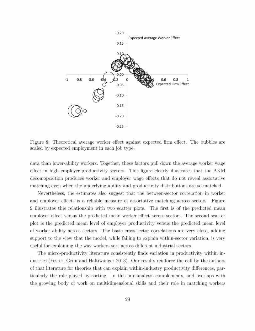
7 Discussion

Our estimates provide support for the central intuition that assortative matching may be

masked by a non-monotone relationship between wage offers and ability. Figure 8 illustrates

the non-monotonic relation using a scatter plot of two theoretical moments fit in our model

(the AKM analogues): the estimated average employer wage effect versus the estimated

average worker wage effect, for each sector-productivity class. The bubbles in the Figure

are scaled by the predicted number of matches. As the employer wage effect increases, the

expected worker wage effect increases, hits a maximum, and then decreases. This result

occurs because the predicted employer wage effect is monotonically increasing in employer

productivity. Because of assortative matching, the predicted worker ability is also increasing

with the predicted employer wage effect. As employer productivity increases, the share of

jobs filled by the highest-ability workers also increases. Because the highest-ability work-

ers actually get lower wage offers, they also have lower worker wage effects in their wage

28

‐0.25

‐0.20

‐0.15

‐0.10

‐0.05

0.00

0.05

0.10

0.15

0.20

‐1 ‐0.8 ‐0.6 ‐0.4 ‐0.2 0 0.2 0.4 0.6 0.8 1Expected Firm Effect

Expected Average Worker Effect

Figure 8: Theoretical average worker effect against expected firm effect. The bubbles arescaled by expected employment in each job type.

data than lower-ability workers. Together, these factors pull down the average worker wage

effect in high employer-productivity sectors. This figure clearly illustrates that the AKM

decomoposition produces worker and employer wage effects that do not reveal assortative

matching even when the underlying ability and productivity distributions are so matched.

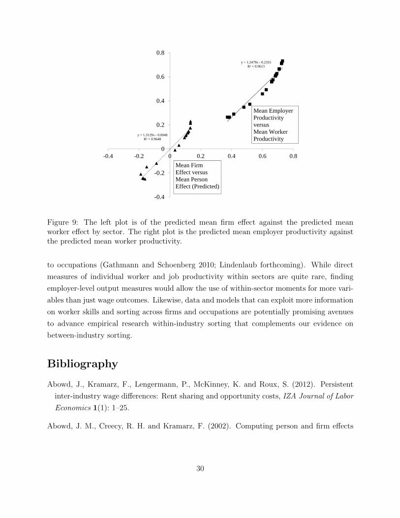
Nevertheless, the estimates also suggest that the between-sector correlation in worker

and employer effects is a reliable measure of assortative matching across sectors. Figure

9 illustrates this relationship with two scatter plots. The first is of the predicted mean

employer effect versus the predicted mean worker effect across sectors. The second scatter

plot is the predicted mean level of employer productivity versus the predicted mean level

of worker ability across sectors. The basic cross-sector correlations are very close, adding

support to the view that the model, while failing to explain within-sector variation, is very

useful for explaining the way workers sort across different industrial sectors.

The micro-productivity literature consistently finds variation in productivity within in-

dustries (Foster, Grim and Haltiwanger 2013). Our results reinforce the call by the authors

of that literature for theories that can explain within-industry productivity differences, par-

ticularly the role played by sorting. In this our analysis complements, and overlaps with

the growing body of work on multidimensional skills and their role in matching workers

29

y = 1.3129x - 0.0048R² = 0.9648

y = 1.2479x - 0.2355R² = 0.9613

-0.4

-0.2

0

0.2

0.4

0.6

0.8

-0.4 -0.2 0 0.2 0.4 0.6 0.8

Mean Employer Productivity versus Mean Worker Productivity

Mean FirmEffect versus Mean Person Effect (Predicted)

Figure 9: The left plot is of the predicted mean firm effect against the predicted meanworker effect by sector. The right plot is the predicted mean employer productivity againstthe predicted mean worker productivity.

to occupations (Gathmann and Schoenberg 2010; Lindenlaub forthcoming). While direct

measures of individual worker and job productivity within sectors are quite rare, finding

employer-level output measures would allow the use of within-sector moments for more vari-

ables than just wage outcomes. Likewise, data and models that can exploit more information

on worker skills and sorting across firms and occupations are potentially promising avenues

to advance empirical research within-industry sorting that complements our evidence on

between-industry sorting.

Bibliography

Abowd, J., Kramarz, F., Lengermann, P., McKinney, K. and Roux, S. (2012). Persistent

inter-industry wage differences: Rent sharing and opportunity costs, IZA Journal of Labor

Economics 1(1): 1–25.

Abowd, J. M., Creecy, R. H. and Kramarz, F. (2002). Computing person and firm effects

30

using linked longitudinal employer-employee data, Technical Report TP-2002-06, LEHD,

U.S. Census Bureau.

Abowd, J. M., Gittings, K., McKinney, K. L., Stephens, B. E., Vilhuber, L. and Woodcock,

S. (2012). Dynamically consistent noise infusion as confidentiality protection, Proceedings

of the Federal Committee on Statistical Metholology, Federal Committee on Statistical

Metholology.

Abowd, J. M. and Kramarz, F. (1999). The analysis of labor markets using matched

employer-employee data, in O. Ashenfelter and D. Card (eds), Handbook of Labor Eco-

nomics, Vol. 3 of Handbook of Labor Economics, Elsevier, chapter 40, pp. 2629–2710.

Abowd, J. M., Kramarz, F. and Margolis, D. N. (1999). High wage workers and high wage

firms, Econometrica 67(2): 251–333.

Abowd, J. M., Lengermann, P. and McKinney, K. L. (2003). The measurement of human

capital in the U.S. economy, Technical Report TP-2002-09, LEHD, U.S. Census Bureau.

Abowd, J. M. and Schmutte, I. M. (2015). Endogenous mobility, Cornell University School

of Industrial and Labor Relations .

Bartolucci, C. and Devicienti, F. (2012). Better workers move to better firms: A simple test

to identify sorting, Carlo Alberto Notebooks 259, Collegio Carlo Alberto.

Becker, G. S. (1973). A theory of marriage: Part I, Journal of Political Economy 81(4): 813–

46.

Card, D., Cardoso, A. R. and Kline, P. (2016). Bargaining, sorting, and the gender wage

gap: Quantifying the impact of firms on the relative pay of women, The Quarterly Journal

of Economics 131(2): 633.

Card, D., Heining, J. and Kline, P. (2013). Workplace Heterogeneity and the Rise of West

German Wage Inequality, The Quarterly Journal of Economics 128(3): 967–1015.

Davis, S. J., Faberman, R. J. and Haltiwanger, J. C. (2013). The Establishment-Level

Behavior of Vacancies and Hiring, The Quarterly Journal of Economics 128(2): 581–622.

Eeckhout, J. and Kircher, P. (2011). Identifying sorting–in theory, Review of Economic

Studies 78(3): 872–906.

31

Foster, L., Grim, C. and Haltiwanger, J. (2013). Reallocation in the Great Recession: Cleans-

ing or not?, Labor Markets in the Aftermath of the Great Recession, NBER Chapters,

National Bureau of Economic Research, Inc, pp. 293–331.

Gathmann, C. and Schoenberg, U. (2010). How general is human capital? A task-based

approach, Journal of Labor Economics 28(1): 1–49.

Goffe, W. L., Ferrier, G. D. and Rogers, J. (1994). Global optimization of statistical functions

with simulated annealing, Journal of Econometrics 60: 65–99.

Golub, G. and Loan, C. (1996). Matrix computations, Johns Hopkins studies in the mathe-

matical sciences, Johns Hopkins University Press.

Hagedorn, M., Law, T. H. and Manovskii, I. (2017). Identifying equilibrium models of labor

market sorting, Econometrica 85(1): 29–65.

Hornstein, A., Krusell, P. and Violante, G. L. (2011). Frictional wage dispersion in search

models: A quantitative assessment, American Economic Review 101(7): 2873–98.

Ingber, L. (1993). Adaptive simulated annealing (ASA) global optimization C-code, Tech-

nical report, Caltech Alumni Association.

Iranzo, S., Schivardi, F. and Tosetti, E. (2008). Skill dispersion and firm productivity: An

analysis with matched employer-employee data, Journal of Labor Economics 26: 247–285.

Kennes, J. and le Maire, D. (2013). Job heterogeneity and coordination frictions, Economics

Working Papers 2013-09, School of Economics and Management, University of Aarhus.

Lindenlaub (forthcoming). Sorting multidimensional types: Theory and application, Review

of Economic Studies .

Lise, J., Meghir, C. and Robin, J.-M. (2016). Matching, sorting and wages, Review of

Economic Dynamics 19: 63 – 87. Special Issue in Honor of Dale Mortensen.

Lopes de Melo, R. (forthcoming). Firm wage differentials and labor market sorting: Recon-

ciling theory and evidence, Journal of Political Economy .

Mortensen, D. T. (2003). Wage Dispersion: Why Are Similar Workers Paid Differently,

Zeuthen lecture book series, MIT Press.

32

Ruud, P. A. (2000). An Introduction to Classical Econometric Theory, Oxford University

Press.

Sakata, S. and White, H. (2001). S-estimation of nonlinear regression models with dependent

and heterogeneous observations, Journal of Econometrics 103: 5–72.

Shimer, R. (2005). The assignment of workers to jobs in an economy with coordination

frictions, Journal of Political Economy 113: 996.

Shimer, R. and Smith, L. (2000). Assortative Matching and Search, Econometrica

68(2): 343–370.

Slichter, S. H. (1950). Notes on the structure of wages, Review of Economics and Statistics

32(1): 80–91.

Thaler, R. H. (1989). Interindustry wage differentials, Journal of Economic Perspectives

3(2): 181–193.

Woodcock, S. (2008). Wage differentials in the presence of unobserved worker, firm, and

match heterogeneity, Labour Economics 15: 772–794.

33

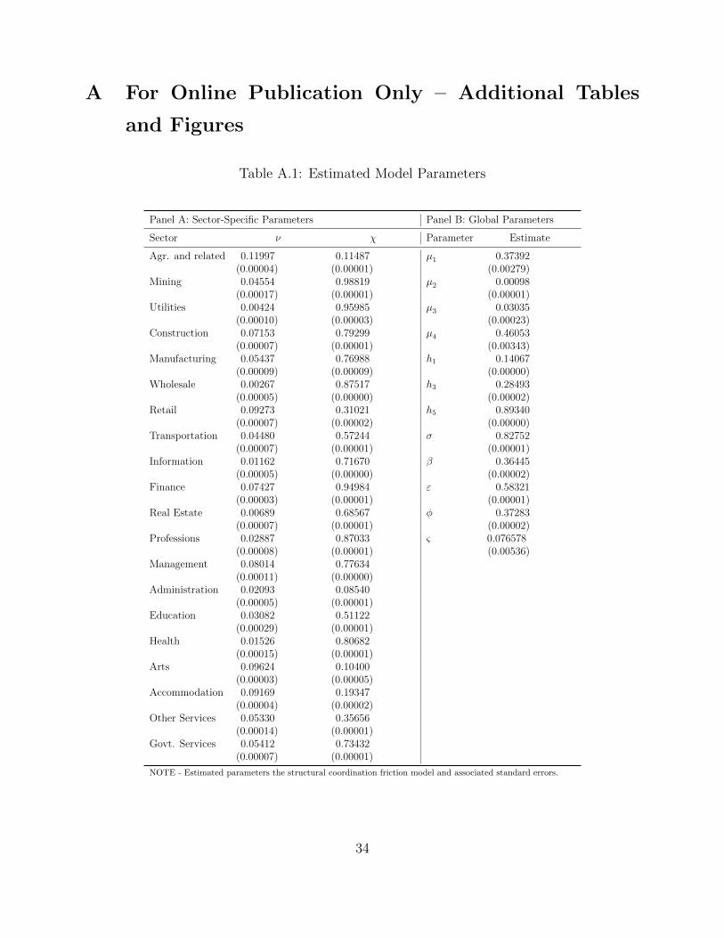
A For Online Publication Only – Additional Tables

and Figures

Table A.1: Estimated Model Parameters

Panel A: Sector-Specific Parameters Panel B: Global Parameters

Sector ν χ Parameter Estimate

Agr. and related 0.11997 0.11487 µ1 0.37392(0.00004) (0.00001) (0.00279)

Mining 0.04554 0.98819 µ2 0.00098(0.00017) (0.00001) (0.00001)

Utilities 0.00424 0.95985 µ3 0.03035(0.00010) (0.00003) (0.00023)

Construction 0.07153 0.79299 µ4 0.46053(0.00007) (0.00001) (0.00343)

Manufacturing 0.05437 0.76988 h1 0.14067(0.00009) (0.00009) (0.00000)

Wholesale 0.00267 0.87517 h3 0.28493(0.00005) (0.00000) (0.00002)

Retail 0.09273 0.31021 h5 0.89340(0.00007) (0.00002) (0.00000)

Transportation 0.04480 0.57244 σ 0.82752(0.00007) (0.00001) (0.00001)

Information 0.01162 0.71670 β 0.36445(0.00005) (0.00000) (0.00002)

Finance 0.07427 0.94984 ε 0.58321(0.00003) (0.00001) (0.00001)

Real Estate 0.00689 0.68567 φ 0.37283(0.00007) (0.00001) (0.00002)

Professions 0.02887 0.87033 ς 0.076578(0.00008) (0.00001) (0.00536)

Management 0.08014 0.77634(0.00011) (0.00000)

Administration 0.02093 0.08540(0.00005) (0.00001)

Education 0.03082 0.51122(0.00029) (0.00001)

Health 0.01526 0.80682(0.00015) (0.00001)

Arts 0.09624 0.10400(0.00003) (0.00005)

Accommodation 0.09169 0.19347(0.00004) (0.00002)

Other Services 0.05330 0.35656(0.00014) (0.00001)

Govt. Services 0.05412 0.73432(0.00007) (0.00001)

NOTE - Estimated parameters the structural coordination friction model and associated standard errors.

34

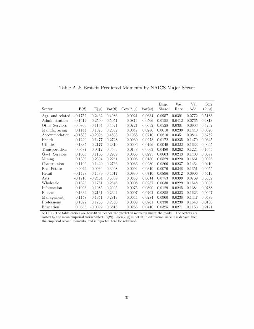
Table A.2: Best-fit Predicted Moments by NAICS Major Sector

Emp. Vac. Val. CorrSector E(θ) E(ψ) Var(θ) Cov(θ, ψ) Var(ψ) Share Rate Add. (θ, ψ)

Agr. and related -0.1752 -0.2432 0.4986 0.0921 0.0634 0.0957 0.0391 0.0772 0.5183Administration -0.1612 -0.2500 0.5051 0.0814 0.0566 0.0158 0.0412 0.0765 0.4813Other Services -0.0866 -0.1194 0.4521 0.0721 0.0652 0.0528 0.0301 0.0963 0.4202Manufacturing 0.1144 0.1323 0.2832 0.0047 0.0286 0.0610 0.0239 0.1440 0.0520Accommodation -0.1883 -0.2095 0.4833 0.1068 0.0710 0.0810 0.0351 0.0814 0.5762Health 0.1220 0.1477 0.2728 0.0030 0.0278 0.0172 0.0235 0.1479 0.0345Utilities 0.1335 0.2177 0.2319 0.0006 0.0196 0.0049 0.0222 0.1633 0.0095Transportation 0.0587 0.0312 0.3533 0.0188 0.0363 0.0480 0.0262 0.1224 0.1655Govt. Services 0.1065 0.1166 0.2939 0.0065 0.0295 0.0603 0.0243 0.1403 0.0697Mining 0.1339 0.2304 0.2251 0.0006 0.0180 0.0529 0.0220 0.1661 0.0096Construction 0.1192 0.1420 0.2766 0.0036 0.0280 0.0806 0.0237 0.1464 0.0410Real Estate 0.0944 0.0936 0.3098 0.0094 0.0310 0.0076 0.0248 0.1351 0.0955Retail -0.1498 -0.1489 0.4617 0.0980 0.0710 0.0896 0.0312 0.0906 0.5413Arts -0.1710 -0.2464 0.5009 0.0888 0.0614 0.0753 0.0399 0.0769 0.5062Wholesale 0.1323 0.1761 0.2546 0.0008 0.0257 0.0030 0.0229 0.1548 0.0098Information 0.1023 0.1085 0.2995 0.0075 0.0300 0.0129 0.0245 0.1384 0.0788Finance 0.1334 0.2131 0.2344 0.0007 0.0202 0.0858 0.0223 0.1623 0.0097Management 0.1158 0.1351 0.2813 0.0044 0.0284 0.0900 0.0238 0.1447 0.0489Professions 0.1322 0.1736 0.2560 0.0008 0.0261 0.0330 0.0230 0.1543 0.0100Education 0.0335 -0.0092 0.3815 0.0265 0.0410 0.0325 0.0271 0.1153 0.2121

NOTE - The table entries are best-fit values for the predicted moments under the model. The sectors aresorted by the mean empirical worker-effect, E(θ)). Corr(θ, ψ) is not fit in estimation since it is derived fromthe empirical second moments, and is reported here for reference.

35

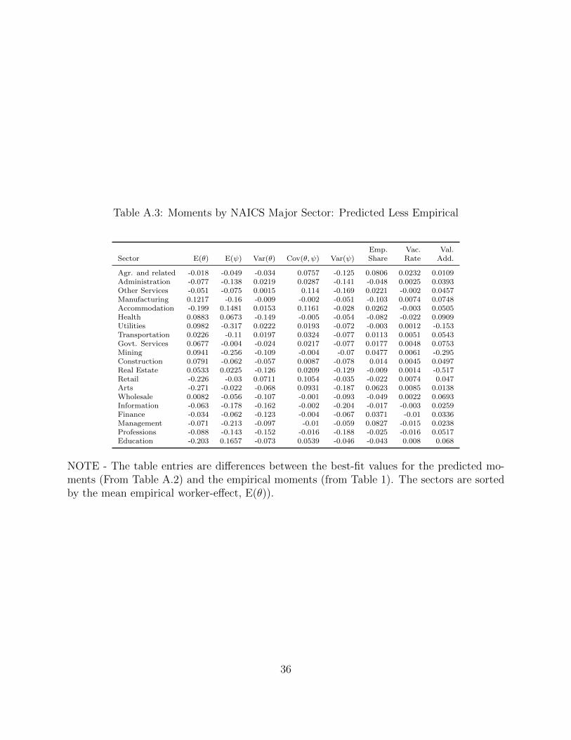
Table A.3: Moments by NAICS Major Sector: Predicted Less Empirical

Emp. Vac. Val.Sector E(θ) E(ψ) Var(θ) Cov(θ, ψ) Var(ψ) Share Rate Add.

Agr. and related -0.018 -0.049 -0.034 0.0757 -0.125 0.0806 0.0232 0.0109Administration -0.077 -0.138 0.0219 0.0287 -0.141 -0.048 0.0025 0.0393Other Services -0.051 -0.075 0.0015 0.114 -0.169 0.0221 -0.002 0.0457Manufacturing 0.1217 -0.16 -0.009 -0.002 -0.051 -0.103 0.0074 0.0748Accommodation -0.199 0.1481 0.0153 0.1161 -0.028 0.0262 -0.003 0.0505Health 0.0883 0.0673 -0.149 -0.005 -0.054 -0.082 -0.022 0.0909Utilities 0.0982 -0.317 0.0222 0.0193 -0.072 -0.003 0.0012 -0.153Transportation 0.0226 -0.11 0.0197 0.0324 -0.077 0.0113 0.0051 0.0543Govt. Services 0.0677 -0.004 -0.024 0.0217 -0.077 0.0177 0.0048 0.0753Mining 0.0941 -0.256 -0.109 -0.004 -0.07 0.0477 0.0061 -0.295Construction 0.0791 -0.062 -0.057 0.0087 -0.078 0.014 0.0045 0.0497Real Estate 0.0533 0.0225 -0.126 0.0209 -0.129 -0.009 0.0014 -0.517Retail -0.226 -0.03 0.0711 0.1054 -0.035 -0.022 0.0074 0.047Arts -0.271 -0.022 -0.068 0.0931 -0.187 0.0623 0.0085 0.0138Wholesale 0.0082 -0.056 -0.107 -0.001 -0.093 -0.049 0.0022 0.0693Information -0.063 -0.178 -0.162 -0.002 -0.204 -0.017 -0.003 0.0259Finance -0.034 -0.062 -0.123 -0.004 -0.067 0.0371 -0.01 0.0336Management -0.071 -0.213 -0.097 -0.01 -0.059 0.0827 -0.015 0.0238Professions -0.088 -0.143 -0.152 -0.016 -0.188 -0.025 -0.016 0.0517Education -0.203 0.1657 -0.073 0.0539 -0.046 -0.043 0.008 0.068

NOTE - The table entries are differences between the best-fit values for the predicted mo-ments (From Table A.2) and the empirical moments (from Table 1). The sectors are sortedby the mean empirical worker-effect, E(θ)).

36

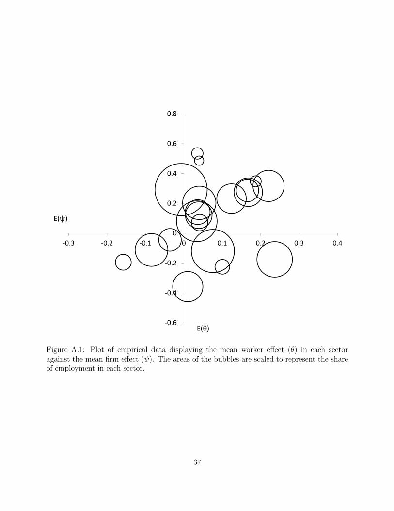
‐0.6

‐0.4

‐0.2

0

0.2

0.4

0.6

0.8

‐0.3 ‐0.2 ‐0.1 0 0.1 0.2 0.3 0.4

E(ψ)

E(θ)

Figure A.1: Plot of empirical data displaying the mean worker effect (θ) in each sectoragainst the mean firm effect (ψ). The areas of the bubbles are scaled to represent the shareof employment in each sector.

37

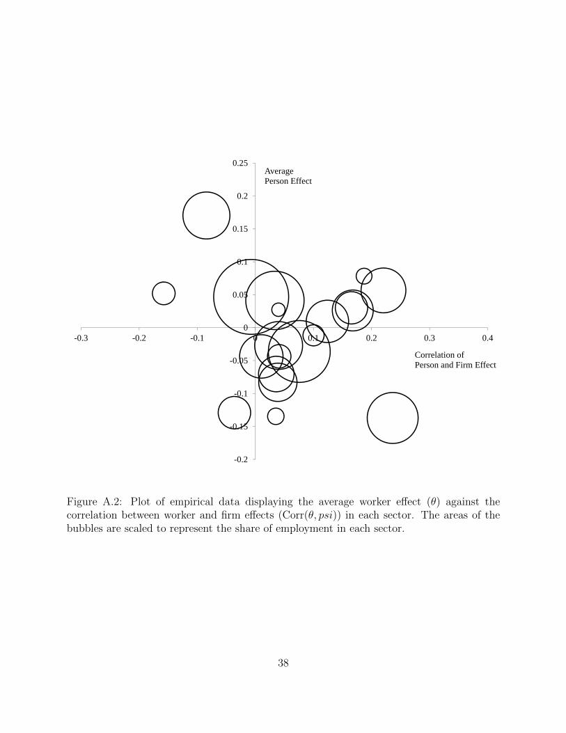
-0.2

-0.15

-0.1

-0.05

0

0.05

0.1

0.15

0.2

0.25

-0.3 -0.2 -0.1 0 0.1 0.2 0.3 0.4

AveragePerson Effect

Correlation ofPerson and Firm Effect

Figure A.2: Plot of empirical data displaying the average worker effect (θ) against thecorrelation between worker and firm effects (Corr(θ, psi)) in each sector. The areas of thebubbles are scaled to represent the share of employment in each sector.

38

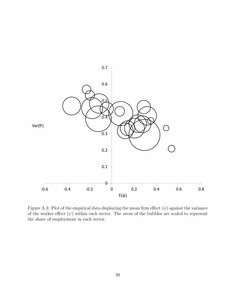
0

0.1

0.2

0.3

0.4

0.5

0.6

0.7

‐0.6 ‐0.4 ‐0.2 0 0.2 0.4 0.6 0.8

Var(θ

E(ψ)

Figure A.3: Plot of the empirical data displaying the mean firm effect (ψ) against the varianceof the worker effect (ψ) within each sector. The areas of the bubbles are scaled to representthe share of employment in each sector.

39

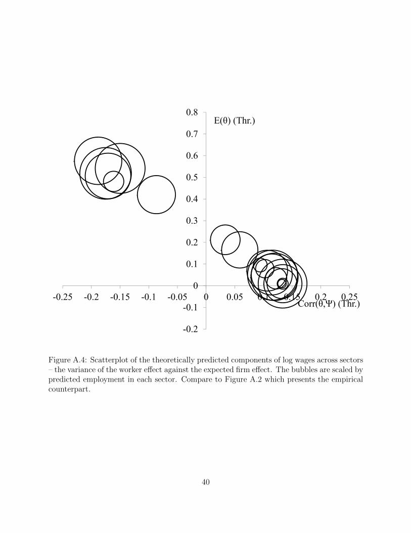
-0.2

-0.1

0

0.1

0.2

0.3

0.4

0.5

0.6

0.7

0.8

-0.25 -0.2 -0.15 -0.1 -0.05 0 0.05 0.1 0.15 0.2 0.25

E(θ) (Thr.)

Corr(θ,Ψ) (Thr.)

Figure A.4: Scatterplot of the theoretically predicted components of log wages across sectors– the variance of the worker effect against the expected firm effect. The bubbles are scaled bypredicted employment in each sector. Compare to Figure A.2 which presents the empiricalcounterpart.

40

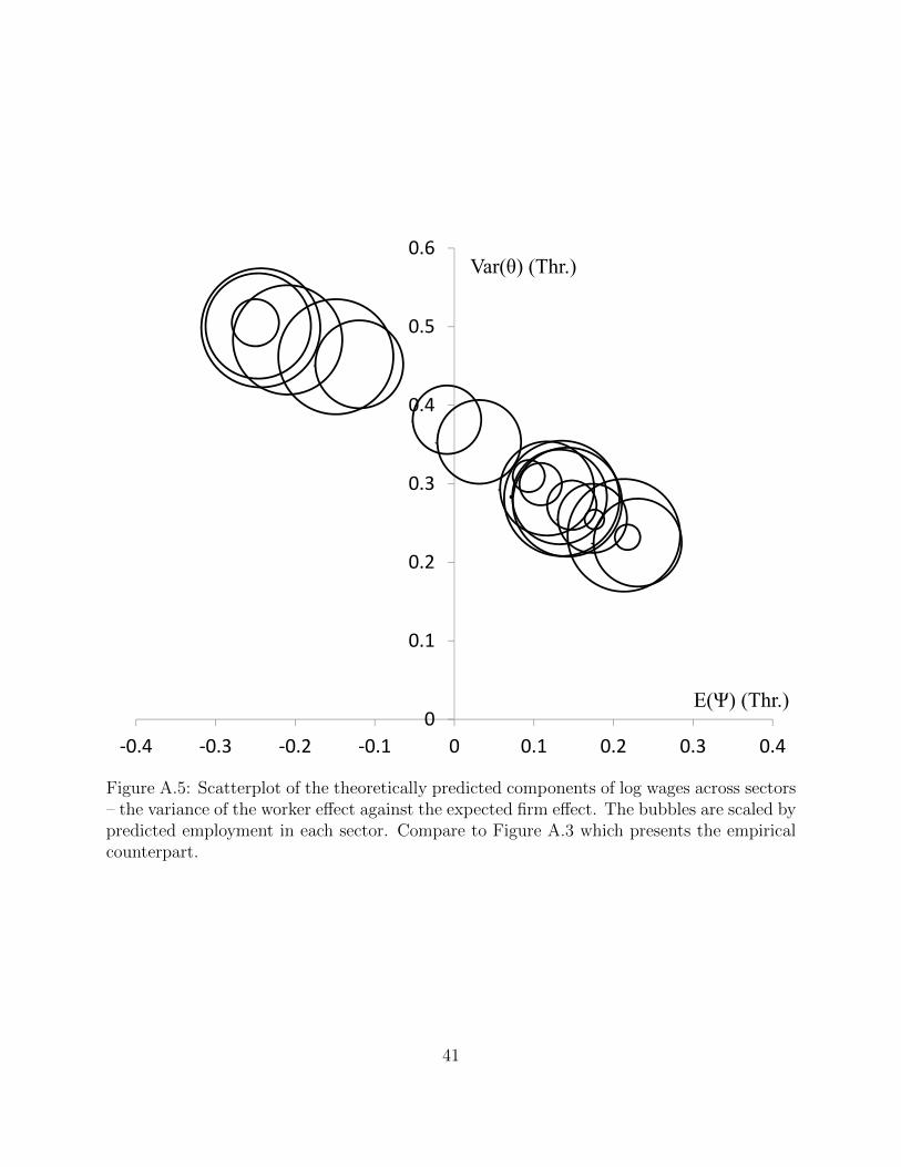
0

0.1

0.2

0.3

0.4

0.5

0.6

‐0.4 ‐0.3 ‐0.2 ‐0.1 0 0.1 0.2 0.3 0.4

Var(θ) (Thr.)

E(Ψ) (Thr.)

Figure A.5: Scatterplot of the theoretically predicted components of log wages across sectors– the variance of the worker effect against the expected firm effect. The bubbles are scaled bypredicted employment in each sector. Compare to Figure A.3 which presents the empiricalcounterpart.

41

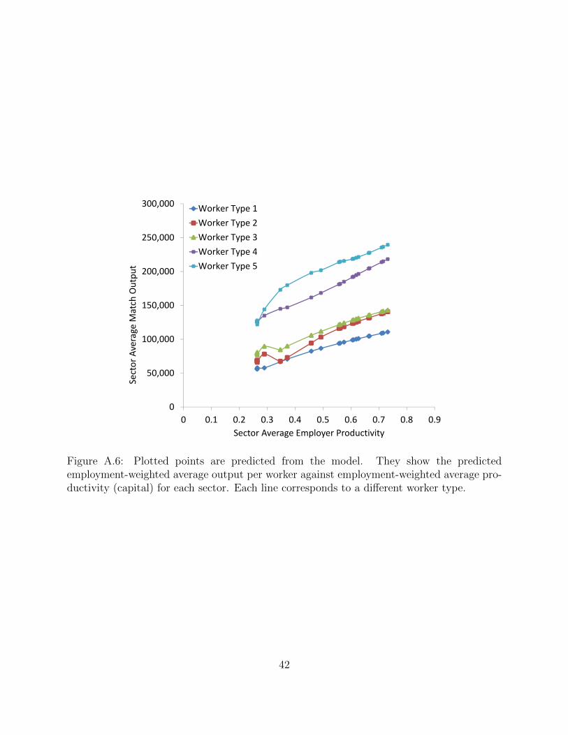
0

50,000

100,000

150,000

200,000

250,000

300,000

0 0.1 0.2 0.3 0.4 0.5 0.6 0.7 0.8 0.9

Sector Average M

atch Outpu

t

Sector Average Employer Productivity

Worker Type 1Worker Type 2Worker Type 3Worker Type 4Worker Type 5

Figure A.6: Plotted points are predicted from the model. They show the predictedemployment-weighted average output per worker against employment-weighted average pro-ductivity (capital) for each sector. Each line corresponds to a different worker type.

42

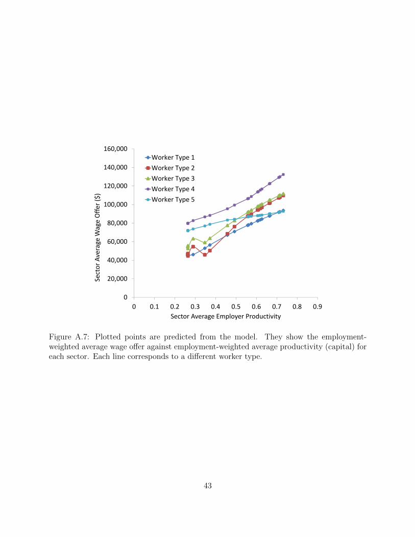
0

20,000

40,000

60,000

80,000

100,000

120,000

140,000

160,000

0 0.1 0.2 0.3 0.4 0.5 0.6 0.7 0.8 0.9

Sector Average W

age Offe

r ($)

Sector Average Employer Productivity

Worker Type 1Worker Type 2Worker Type 3Worker Type 4Worker Type 5

Figure A.7: Plotted points are predicted from the model. They show the employment-weighted average wage offer against employment-weighted average productivity (capital) foreach sector. Each line corresponds to a different worker type.

43

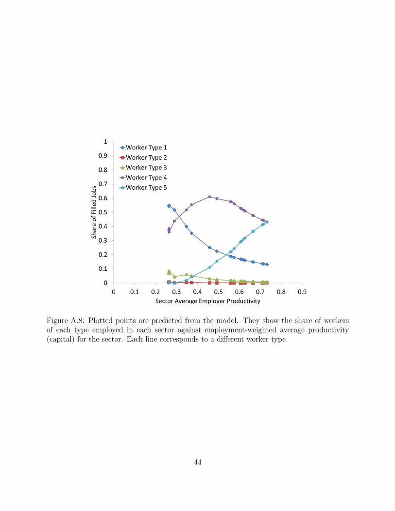
0

0.1

0.2

0.3

0.4

0.5

0.6

0.7

0.8

0.9

1

0 0.1 0.2 0.3 0.4 0.5 0.6 0.7 0.8 0.9

Share of Filled

Jobs

Sector Average Employer Productivity

Worker Type 1Worker Type 2Worker Type 3Worker Type 4Worker Type 5

Figure A.8: Plotted points are predicted from the model. They show the share of workersof each type employed in each sector against employment-weighted average productivity(capital) for the sector. Each line corresponds to a different worker type.

44

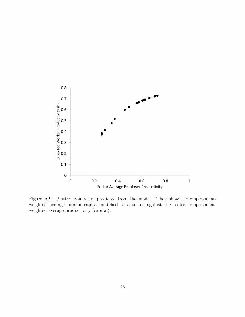
0

0.1

0.2

0.3

0.4

0.5

0.6

0.7

0.8

0 0.2 0.4 0.6 0.8 1

Expe

cted

Worker P

rodu

ctivity

(h)

Sector Average Employer Productivity

Figure A.9: Plotted points are predicted from the model. They show the employment-weighted average human capital matched to a sector against the sectors employment-weighted average productivity (capital).

45

B For Online Publication Only – Data Appendix

We use data from the Longitudinal Employer-Household Dynamics Program (LEHD), uni-

verse data for twenty-eight large American states with information from 1990-2004. Our

analysis sample is restricted to individuals aged 18-70, employed full-time at their dominant

employer. The following sections describe the underlying microdata sources and how we

construct the analysis variables and impose sample restrictions.

B.1 Unemployment Insurance

The individual data were derived from the universe of unemployment insurance (UI) quar-

terly wage records from twenty-eight states.26 The BLS Handbook of Methods (1997) de-

scribes UI coverage as “broad and basically comparable from state to state,” and claims over

96 percent of total wage and salary civilian nonfarm jobs were covered in 1994. The Federal

Unemployment Tax Act (FUTA), first enacted in 1938, lays the ground rules for the kinds

of employment which must be covered in state unemployment insurance laws. While tech-

nically mandating coverage of all employers with one or more employees in a calendar year,

FUTA allows for numerous exceptions to covered employment. These include workers at

small agricultural co-operatives, employees of the federal government, and certain employees

of state governments, most notably elected officials, members of the judiciary, and emergency

workers. According to the Handbook, UI wage records measure “gross wages and salaries,

bonuses, stock options, tips, and other gratuities, and the value of meals and lodging, where

supplied.” They do not include OASDI, health insurance, workers compensation, unemploy-

ment insurance, and private pension and welfare funds. Individuals are uniquely identified

and followed for all quarters in which their employers had reporting requirements in the UI

system. Thus, cross-state mobility can be observed for individuals moving between any of

states for which we have data. Although coverage dates vary, all states provide between

seven and thirteen years of data. In our analysis, by combining them into a single “pooled”

file, we have information on approximately 190 million workers, 10 million employers, and

660 million annual earnings records.

26We cannot disclose which states are included in the analysis as a condition imposed by the Census Bureauon the public use data. We can, however, release the moment matrices used in the structural estimation,upon request, as they have been designated as public-use data.

46

B.2 Creation of Variables

Using Census Bureau and other LEHD data bases, sex, race, and date of birth are com-

bined with the individual earnings data using an exact match to administrative Upon each

individual’s first appearance in the data, labor force experience as potential labor force ex-

perience (age - education - 6) is calculated. In subsequent periods, experience is measured

as the sum of observed experience and initial (potential) experience. The UI wage records

connect individuals to every employer from which they received wages in any quarter of a

given calendar year. Therefore, individual employment histories are constructed using the

same personal identifier used in the individual data. Employers are identified by their state

unemployment insurance account number (SEIN). While large employers undoubtedly op-

erate in multiple states, their SEINs are unfortunately state specific, meaning they cannot

be connected. In addition, while we match workers to their employers, it is not possible

to connect those employed in firms with multiple establishments to specific places of work.

This problem is not overly pervasive, as over 70% of employment occurs in firms with only

a single establishment.

B.3 Earnings

For every year an individual appears in a state, a “dominant” employer — the employer for

whom the sum of quarterly earnings is the highest—is identified in order to better approx-

imate the individual’s full-time, full-year annual wage rate using the following steps. First,

define full quarter employment in quarter t as having an employment history with positive

earnings for quarters t − 1, t, and t + 1. Continuous employment during quarter t means

having an employment history with positive earnings for either t − 1 and t or t and t + 1.

Employment spells that are neither full quarter nor continuous are designated discontinuous.

If the individual was full quarter employed for at least one quarter at the dominant employer,

the annualized wage is computed as 4 times average full quarter earnings at that employer

(total full quarter earnings divided by the number of full quarters worked). This accounts for

84% of the person-year-state observations in our eventual analysis sample. Otherwise, if the

individual was continuously employed for at least one quarter at the dominant employer, the

annualized wage is average earnings in all continuous quarters of employment at the domi-

nant employer multiplied by 8 (i.e., 4 quarters divided by an expected employment duration

during the continuous quarters of 0.5). This accounts for 11% of all observations. For the

remaining 5%, annualized wages are average earnings in each quarter multiplied by 12 (i.e.,

47

4 quarters divided by an expected employment duration during discontinuous quarters of

0.33).

B.4 Annual Hours of Work and Full-time Status

We restrict our sample to individuals who worked full-time for their dominant employer.

Full-time status is taken to mean that the individual worked at least 35 hours per week. The

average number of hours per week for a worker is given by dividing the number of hours

worked over the year with the dominant employer by the number of weeks worked. The

number of weeks worked is approximated based on the observed number of full, continuous,

and discontinuous quarters with one’s dominant employer. Specifically, we compute weeks

worked as 13 times the number of full quarters + 6.5 times the number of continuous quarters

+ 4.33 times the number of discontinuous quarters. Annual hours of work are observed for a

subset of individuals in the sample via a database link to other LEHD and Census sources.

For those missing annual hours of work, a value is statistically assigned using a Bayesian

multiple imputation procedure.

B.5 Human Capital Estimates

To the dominant job frame, we attach the variance components of earnings estimated from

the Abowd et al. (1999) human capital decomposition. The estimation of those variance

components in the LEHD data is the subject of another paper, Abowd et al. (2002), to

which we refer the interested reader.

C For Online Publication Only – An Economy with

Heterogeneous Workers and Firms

In this Appendix we derive worker and firm effects in an economy with only two types of

workers and a continuum of firms differing by size and production technology. Notation in

this appendix differs slightly from the notation in the main paper in order to accommodate

the more general specification.

48

C.1 The Economy

Let the economy consist of two types of workers. This is not as limiting as it sounds, for it

may only represent heterogeneity inside a particular class of workers since we consider the

effects net of observables. The economy is divided in a finite number k of industries. The

workers are hired by a continuum of firms, indexed by the share x of type 1 workers each

firm hires, the size t of the firm, and the industry k. The share x is unobserved by the

econometrician. In industry k, there is a mass (density) µk(x, t) of firms of type (k, x, t). We

omit from what follows the k index except when it is necessary.

The economy as a whole is represented by the space Ω = Ω1, . . . ,Ωk with Ωk = [0, 1]×R+, the space defining each industry. There is a quantity (or number) J =

∫Ωdµ of firms,

Jk =∫

Ωkdµk in each industry. Firm (x, t) hires xt of type 1 workers, and (1− x)t of type 2.

We write∫

Ωxt dµ(x, t) = M and

∫Ω

(1 − x)t dµ(x, t) = N so that there are M + N workers

in the economy. Type 1 workers earn w(x, t, k) in firm (x, t) in industry k while type 2 earn

u(x, t, k); the wage only depends on the industry, the share of type 1 workers, and the size

of the firm.

C.2 The Economy as Estimated by Person and Firm Effects

As in Abowd et al. (1999) (hereafter, AKM99), decompose the individual wage, lnwi,j(i,t),t,

after conditioning for observables, in each period as the sum of an individual effect, θi, a

firm effect, ψj(i,t), and a residual, εi,j(i),t

lnwi,j(i,t),t = θi + ψj(i,t) + εi,j(i),t

We consider here only the limiting (and purely theoretical) case where the number of time

periods goes to infinity and the workers visit ergodically all firms and all industries. This

frees us from the identification problem discussed in detail in the above paper. Moreover,

the effects estimated in AKM99 would converge in probability to the theoretical values we

show below.

In this case, even though the type of the worker is not directly known by the econome-

trician, observing the workers jump from job to job provides enough information to be able

to reduce the above ordinary least squares (OLS) problem to the following minimization

problem. Find W , U (worker effects) and ψ(k, x, t) (firm effect in industry k for a firm of

49

size t hiring a proportion x of type 1 workers) that solve

minW,U,ψ

∫Ω

[xt (w(x, t)−W − ψ(x, t))2 + (1− x)t (u(x, t)− U − ψ(x, t))2] dµ(x, t). (17)

This problem is exactly equivalent to minimizing the sum of squared residuals in ordinary

least squares. The solutions to this problem are unique up to a constant. We show that:

Theorem 2 Under integrability assumptions on w and u, the solutions to the OLS program

(17) are of the type

W =

∫x(1− x)tw(x, t)∫

x(1− x)t+ Λ, (18)

U =

∫x(1− x)tu(x, t)∫

x(1− x)t+ Λ, (19)

ψ(x, t) = x(w(x, t)−W ) + (1− x)(u(x, t)− U)− Λ (20)

where the integrals are all taken on Ω with respect to the measure µ, and Λ is an arbitrary

constant (we will set Λ = 0 in the rest of the paper).

Proof. Set U = 0 for the time being, as the solutions are only identified up to a constant.

Let us write J(W,ψ) =∫

Ωρ(W,ψ)(x, t) dµ(x, t). J is defined on R×L2(Ω, µ), and may take

the value +∞. It is clear that ρ is convex in its two arguments (as sum of two squares);

hence J is also convex, and can be show to be strictly convex if w(x, t) − u(x, t) is not a

constant. Hence it has a unique minimum under this assumption, characterized by the first

order constraints ∫Ω

xt(w(x, t)−W − ψ(x, t)) dµ(x, t) = 0 (21)∫Ω

xt(w(x, t)−W − ψ(x, t)) + (1− x)t(u(x, t)− ψ(x, t)) = 0 (22)

Hence W =∫xt(w − ψ) dµ/

∫xt dB and ψ = x(w −W ) + (1 − x)u. Replacing ψ by this

last value in equation 21 and simplifying with the fact that∫x2t = M −

∫x(1 − x)t and∫

x2tw =∫xtw −

∫x(1− x)w proves the theorem.

Remark 3 (Some special cases) If all firms hire the same number of both types of workers,

the distribution µk for all k is δ1/2,2, a Dirac distribution of firms of equal size and same

number of type 1 workers. This leads to W =∑

k wk/k, U =∑

k uk/k, ψk = 12(wk − w +

50

uk − u), where wk is the wage in industry k.

The case where the distribution µ has all mass in t at t = 2 and w(x, t) = u(x, t) + δ leads

to W = U + δ and ψ(x, t) = u(x)− U .

We define the firm-employee effects covariances cov(θ, ψ) as∫(xtW + (1− x)tU)ψ(x, t) dµ∫

t dµ−∫

(xtW + (1− x)tU) dµ∫t dµ

∫ψ(x, t) dµ∫t dµ

(23)

For total covariance the integrals are taken over Ω, for within-sector covariance over Ωk for

all k, and the between-sector covariance is the discrete covariance between the means (i.e.

integrals) on the Ωk. Total covariance is as usual the sum of between-sector and within-sector

covariances.

D For Online Publication Only – Computing the The-

oretical Vacancy Rate

To derive the theoretical analogue to the empirical vacancy rates, recall that the empirical

moment measured in JOLTS is

g(s)7 = R(s) = E

(V acj

Empj + V acj|sj = s

),

where the expectation is taken over all firms in sector s. This expression is interpreted as

the probability that a job opening in sector s is left vacant. Under the assignment model,

this expectation is

g(s)7 = Ej|sj=s

(e−Q1j

), (24)

which is the theoretical probability that an open position does not attract any applications

in equilibrium. Since this probability is the same for all employers of the same type, n, we

can rewrite (24) as

Ej|sj=s

(e−Q1,(n,j)

)=

∑Nn=1 ν

(s)n e−Q

(s)1,n∑N

n=1 ν(s)n

.

51

We can express the numerator as the difference between openings and filled openings:

Ej|sj=s

(e−Q1,(n,j)

)=

∑Nn=1 ν

(s)n −

(1− e−Q

(s)1,n

)ν

(s)n∑N

n=1 ν(s)n

. (25)

Because(

1− e−Q(s)1,n

)=∑M

m=1 e−Q(s)

m+1,n(1− e−qm,n), equation (25) simplifies to

γ(s)7 (µ, ν, x) = E(g

(s)7 ) =

∑Nn=1 ν

(s)n −

∑Mm=1

∑Nn=1 λ

(s)m,n∑N

n=1 ν(s)n

. (26)

The structural vacancy rate is equal to the difference between total openings and employment

in sector s as a share of total openings.

E For Online Publication Only – Estimating Equations

Let H(s) be an MN × 1 vector that selects jobs indexed by n ∈ 1, . . . , N that are in sector

s, and let uMN be the MN × 1 unit vector. In these calculations, expectations are taken

with respect to the equilibrium distribution of realized employment matches. The expected

value of θ∗

across matches in sector k, given the model primitives, is

E(g

(s)1

)≡ γ

(s)1 (θ

∗, ψ∗, λ∗) =

∑Mm=1

∑n:s(n)=s λ

∗m,nθ

∗m∑M

m=1

∑n:s(n)=s λ

∗m,n

. (27)

Equation (27) is the match-weighted sum of θ∗

on matches in sector s normalized by the

total measure of such matches. This is more compactly expressed using matrix notation as

γ(s)1

(θ∗, ψ∗, λ∗, x∗

)=H(s)TΛ∗Dθ

∗

H(s)TΛ∗uMN

. (28)

Analogously, the expected value of ψ∗

is

E(g

(s)2

)≡ γ

(s)2

(θ∗, ψ∗, λ∗, x∗

)=H(s)TΛ∗Fψ

∗

H(s)TΛuMN

. (29)

52

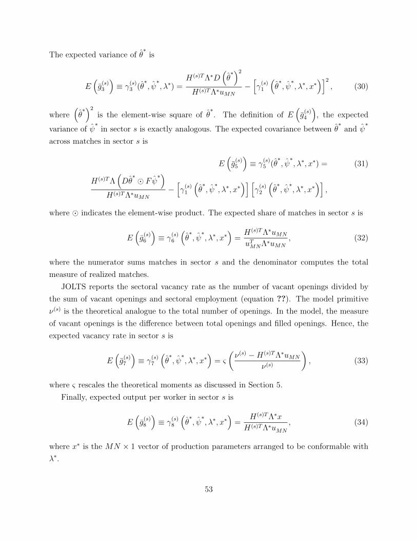
The expected variance of θ∗

is

E(g

(s)3

)≡ γ

(s)3 (θ

∗, ψ∗, λ∗) =

H(s)TΛ∗D(θ∗)2

H(s)TΛ∗uMN

−[γ

(s)1

(θ∗, ψ∗, λ∗, x∗

)]2

, (30)

where(θ∗)2

is the element-wise square of θ∗. The definition of E

(g

(s)4

), the expected

variance of ψ∗

in sector s is exactly analogous. The expected covariance between θ∗

and ψ∗

across matches in sector s is

E(g

(s)5

)≡ γ

(s)5 (θ

∗, ψ∗, λ∗, x∗) = (31)

H(s)TΛ(Dθ∗ Fψ

∗)H(s)TΛ∗uMN

−[γ

(s)1

(θ∗, ψ∗, λ∗, x∗

)] [γ

(s)2

(θ∗, ψ∗, λ∗, x∗

)],

where indicates the element-wise product. The expected share of matches in sector s is

E(g

(s)6

)≡ γ

(s)6

(θ∗, ψ∗, λ∗, x∗

)=H(s)TΛ∗uMN

uTMNΛ∗uMN

, (32)

where the numerator sums matches in sector s and the denominator computes the total

measure of realized matches.

JOLTS reports the sectoral vacancy rate as the number of vacant openings divided by

the sum of vacant openings and sectoral employment (equation ??). The model primitive

ν(s) is the theoretical analogue to the total number of openings. In the model, the measure

of vacant openings is the difference between total openings and filled openings. Hence, the

expected vacancy rate in sector s is

E(g

(s)7

)≡ γ

(s)7

(θ∗, ψ∗, λ∗, x∗

)= ς

(ν(s) −H(s)TΛ∗uMN

ν(s)

), (33)

where ς rescales the theoretical moments as discussed in Section 5.

Finally, expected output per worker in sector s is

E(g

(s)8

)≡ γ

(s)8

(θ∗, ψ∗, λ∗, x∗

)=

H(s)TΛ∗x

H(s)TΛ∗uMN

, (34)

where x∗ is the MN × 1 vector of production parameters arranged to be conformable with

λ∗.

53