Embed Size (px)
Citation preview

1
Source-rock kinetics: the technology, and multiple applications
in hydrocarbon exploration1.
Douglas W. Waples
Sirius Exploration Geochemistry, Inc., 9299 William Cody Drive, Evergreen, CO 80439
e-mail: [email protected]
Acknowledgements
I thank Vincent Nowaczewski for researching closed-system pyrolysis techniques for me. For
personal reasons Vince declined to be recognized formally as a co-author of this paper, but his
contributions, including critiques of the manuscript, were very significant. Any remaining errors
are my responsibility. I also thank Joe Curiale for encouraging me to publish this work in the
Bulletin, Michelle Kominz for creating the sea-level curve, and StratoChem Services for
providing analytical results.
Abstract
The chemical reactions involved directly or indirectly in generation of hydrocarbons from
kerogen are believed to consist mainly of chain reactions that are too complex to be modeled
exactly. However, modeling the overall process of generation as a series of parallel first-order
reactions seems to work well for calculating hydrocarbon generation in basin modeling. The
success of such modeling depends on choosing appropriate kinetic parameters (A factor and
1 Peters et al. (2015) and Waples (submitted) cited an earlier version of this manuscript as “Waples and
Nowaczewski (2013)”. However, due to circumstances beyond my control, that manuscript was never actually published. This paper represents an updated version of that unpublished manuscript. I will be happy to provide a Word® version of the 2013 manuscript to those who want to see the version that was actually referenced.

2
activation-energy (Ea) distribution). The standard pyrolysis methods for determining these
kinetic parameters utilize laboratory data generated at temperatures near 480oC, whereas most
generation in nature occurs at temperatures more than 300oC lower. Appropriate kinetic
parameters will function well at both laboratory and natural temperatures; inappropriate ones
may fit laboratory data well but do not provide reasonable results when applied at basin
temperatures.
Although the multirun pyrolysis method has traditionally been used to derive kinetic parameters,
that approach has often been criticized for sometimes yielding in appropriate kinetic parameters.
I prefer the one-run method, in which the A factor is specified by the user. The one-run method
is faster and less expensive, and is not prone to the potential errors associated with the multirun
method.
Use of the one-run method permits acquisition of larger kinetics data bases, which in turn permit
two new applications of source-rock kinetics, in addition to the traditional application in basin
modeling. The first of these new applications is to organofacies analysis, where the Ea
distributions of different kerogen types and organofacies are distinct. The second new
application is to use the mean activation energies of samples from the same organofacies as
indicators of maturity. Mean Ea for each kerogen type will have different but locally calibratable
correlations with Ro and with Transformation Ratio. Ro equivalents derived from Mean Ea data
can be used to calibrate maturity models, while TR can be used as a direct indicator of the
progress of hydrocarbon generation. Examples of these applications are provided.

3
1. Foundation and definitions
a. Chemical models for kerogen decomposition
The formation of hydrocarbon molecules from a large kerogen molecule must somehow involve
net cleavage of chemical bonds, leading to liberation of small oil and gas molecules, and
alteration of the residual kerogen structure. Cleavage of chemical bonds can in principle occur
via two general types of pathways: simple unimolecular decomposition, in which the bond in
question is stretched enough to eventually break; and multi-center reactions, in which two or
more moieties interact, allowing old bonds to break at the same time that new bonds are formed.
Most workers believe that thermal decomposition of macromolecules, including both polymers
with regular structures and heterogeneous structures like kerogen, occurs via chain reactions.
This statement is fully consistent with the preceding paragraph, since chain reactions consist of
multiple steps that can include both unimolecular and multi-center reactions, as well as
bimolecular (collision) reactions that occur in the chain-propagation and -termination steps.
Excellent descriptions of the vast variety of reactions and reaction sequences that can occur in
chain processes can be found in many discussions of chain reactions.
It is of course possible that hydrocarbon-generation reactions include both simple first-order
decompositions and chain reactions. For example, reactions that occur readily at high laboratory
temperatures may not be as dominant at lower temperatures in geological environments. During
pyrolysis of n-hexane (a chain-reaction sequence where decomposition and hydrogen-transfer
reactions constitute the main portion of the chain), Dominé (1991) noted that hydrogen-transfer
4
reactions were rate limiting at lower temperatures, while decomposition reactions became rate
limiting at higher temperatures.
b. Reaction order and kinetic parameters
Simple decompositions are unimolecular processes that follow first-order kinetics – that is, the
rate of decomposition depends linearly on the concentration [S] of the reacting species S:
Rate = k[S] (1)
where k is the reaction-rate constant for disappearance of S. Multi-center reactions normally
follow second-order kinetics, as in (2), where the two reacting species S1 and S2 can be the
same, but more generally will be different.
Rate = k[S1][S2] (2)
The value of the rate constant k is calculated using the Arrhenius equation (3), which includes
the Arrhenius constant A (also called the A factor or pre-exponential factor), the activation
energy (Ea), and the gas constant R:
k = Aexp(-Ea/RT) (3)
Equation (3) shows that the value of the rate constant k increases as absolute temperature (T)
increases. Because a chain reaction consists of multiple reactions that each have their own value

5
for k, A, and Ea, the overall rate constant k for destruction of a reactant or formation of a product
is normally a mathematically rather unwieldy combination of the A’s and Ea’s for the individual
reactions. Even for decomposition of small, simple molecules like acetaldehyde (CH3CHO), the
rate equations are complex (Benson, 1976, p. 230-231):
Rate = k1*(ki/kt)1/2
*[CH3CHO]3/2
(4)
In equation (4), ki and kt are the rate constants for the chain-initiation and termination reactions,
respectively, and k1 is that for the propagation step. The mechanisms and algebra quickly
become even more complex if we include side reactions (Benson, 1976, pp. 232-233).
The A factor for the overall process of decomposition of acetaldehyde is the product of the A
factors for three different reactions (1, i, and t), and thus will often be significantly different from
the A factor for any of the individual reactions. For example, for acetaldehyde, Benson estimates
that Ai = 1016
s-1
, At = 1010.5
s-1
, and A1 = 108 s
-1. The overall A factor calculated from equation
(4) is 1010.8
s-1
, a value different from the A factor for any of the individual reaction. For systems
that are more complex, including kerogen, any link between the overall A and theory is
essentially non-existent.
Adding to the problem is our standard assumption that the kinetics of kerogen decomposition
follow a first-order rate law, as in equation (1). Acetaldehyde decomposition (equation (4)), in
contrast, follows an overall 3/2 rate law, not unusual for chain reactions. As a result, the A I use
when assuming first-order kinetics will be different than that calculated using equation (4).

6
The same analysis can be carried out to explain why the overall activation energies for chain
reactions are normally lower than those for the individual bond-breaking reactions. It is thus
clear that our kinetic parameters for kerogen decomposition must be determined empirically
rather than from theory.
c. Empirical data relevant to kerogen kinetics
There are several types of laboratory data that can help us choose appropriate A and Ea values
for hydrocarbon formation from kerogen. One such data set represents the A factors for
generation of hydrocarbons from kerogen published by many workers since the late 1980’s. I
have compiled all the data I could find into the histogram shown in Figure 1. All A factors were
determined by the original authors using the standard geochemical technique (discussed below)
of allowing A and Ea to be varied to achieve the best mathematical fit to the laboratory data. The
mean and median values for A in this large and relatively unbiased data set are both about
1.6*1014
s-1
.
Tmax data for kerogens that are at a maturity level just prior to the onset of hydrocarbon
generation can also be used to limit the range of A and Ea that we can expect from kerogens
under natural conditions. The reported range of Tmax values for kerogens at this maturity level
ranges from about 436oC to 446
oC, a span of 10 degrees. A relatively simple algebraic
calculation shows that if all kerogens are assumed to have the same activation energy at peak
generation, this entire variation in observed Tmax can be accounted for by only a change of a
factor of 1.5 in the A factor. On the other hand, if we allow Ea at peak generation to vary over a

7
range of 3 kcal/mole (which in our experience is probably more than enough), then we can
account for the entire range of Tmax values by varying A by about a factor of seven. I therefore
conclude that the natural range of A factors for kerogen decomposition will probably vary by
less than a factor of five.
Alan Burnham (personal communication, 2014) is of the strong opinion that A factors for
kerogens do in fact vary, and vary considerably. I agree that it is implausible that all kerogens
have precisely the same A factor, given the well-documented variations in kerogen structure and
composition. Burnham (personal communication, 2014) also believes that good laboratories can
reproduce A factors for a single sample within a factor of 4, or possibly slightly better.
Combining these various conclusions and opinions, I believe that the great majority of A factors
for hydrocarbon generation from different kerogens can range from about 3*1013
s-1
to 8*1014
s-
1, with a dominance near 2*10
14 s
-1.
d. Parallel reaction model
The process of hydrocarbon generation, whether by simple decomposition or via chain reactions,
must comprise many different simultaneous reactions. These reactions can involve breaking
different types of bonds, as well as breaking the same types of bonds within a variety of chemical
environments within the kerogen structure. When we speak of the rate of hydrocarbon
generation, we are therefore speaking of the sum of the rates of numerous individual reactions,
each of which generates a certain type of hydrocarbon molecule from a specific part of a kerogen
molecule. Equation (1) applied to hydrocarbon generation from kerogen thus becomes

8
Rate = k1[S1] + k2[S2] + … + kn[Sn] (5)
where the k1 is the rate constant for the first generation reaction and [Sn] is the concentration of
the nth and final reactive species. Since we cannot know all the details for all possible reactions,
models are normally simplified by grouping the reactions into a manageable number of
categories – almost always fewer than 20 and often fewer than 10.
e. Activation-energy distribution
Each of the terms in equation (5) represents a distinct group of chemical reactions rather than a
single reaction. Substituting equation (3) into equation (5), we have, at any temperature T,
Rate = A1 exp(-Ea1/RT)[S1] + A2 exp(-Ea2/RT)[S2] + … + An exp(-Ean/RT)[Sn] (6)
where the relative abundances of the reacting species within the kerogen structure vary from
kerogen to kerogen, and change during the process of generation. The individual reactions
bundled into each group may differ in chemistry, but their activation energies are always similar.
From group to group, however, activation energies vary systematically. We thus speak of an
“activation-energy distribution”, where each member (group of reactions) in the distribution is
defined by its average activation energy, and the relative proportion of each group [Si] is also
specified. The great majority of applications today use a standard spacing of 1 kcal/mole
between groups (Fig. 2). Some researchers, however, especially but not limited to the French
Petroleum Institute, have used wider spacing. (e.g., Issler and Snowdon, 1990; Min et al., 2011).

9
Sundararaman et al. (1992), however, showed that 2-kcal spacing could be inadequate, and
advocated 1-kcal spacing. I agree.
By convention, we normally simplify the analysis by assuming that A1 = A2 = … = An (e.g.,
Ungerer and Pelet, 1987). This assumption is supported by Benson (1976, pp. 90-104), who
showed that for typical unimolecular decomposition reactions, A decreases very slightly as
temperature increases over the narrow (<100oC) range of temperatures involved in hydrocarbon
generation. However, Benson’s data also indicate that A increases very slightly as Ea increases.
During natural heating, these two effects largely cancel, lending support to our assumption of
constant A for all activation energies in an Ea distribution (see also Waples, 1996).
Pseudokinetic models and the earliest true-kinetic models, in contrast, generally assumed that A
increased as Ea increased (e.g., Tissot, 1969; Deroo et al., 1969; Ungerer, 1984). More recently,
Min et al. (2011) have also allowed A to vary, although their A values do not change regularly
with Ea.
f. Summary
Activation-energy distributions with a 1-kcal/mole spacing provide a simple, convenient, and
useful model for hydrocarbon generation from kerogen. Wider spacing of Ea values does not
provide the precision required by modern applications of kinetics. Narrower spacing may be
useful in describing Type I kerogens with very narrow Ea distributions (section 2.b.v.)
Combining the various types of relevant data, I conclude that a single A factor of 2*1014
s-1
can
be defended on empirical grounds and used effectively in calculating hydrocarbon generation

10
from all kerogens under natural conditions. This value is slightly higher than the A factor of
1*1014
s-1
previously suggested by Waples et al. (2002, 2010), which also lies within our range
of uncertainty about the true value of A for each kerogen. At the current level of our
understanding, I do not believe that using different A factors for different kerogens, or different
A factors for different activation energies in the Ea distribution, improves accuracy or
convenience in applications of source-rock kinetics. Kinetics with A factors below about 3*1013
s-1
or above about 8*1014
s-1
(e.g., Fig. 2) should either be converted to kinetics with an
acceptable A factor, or else not used.
2. Historical perspective
a. Kinetics prior to 1987
i. Kinetics from pyrolysis of coals and oil shales
The earliest kinetic descriptions of hydrocarbon generation came from studies of the pyrolysis of
coals and oil shales (see Waples, 1984, for a detailed review). Those studies were interested in
commercial retorting, however, and gave no thought to using kinetics to model hydrocarbon
generation under geologic conditions. Therefore, their empirical data apply only to high-
temperature processes, and are of no direct interest for petroleum exploration. In fact, as Deroo et
al. (1969) and Waples (1984) pointed out, these mathematical descriptions were widely
recognized even at that time as “pseudokinetics” rather than true kinetics.
The early pseudokinetics all used a single activation energy, rather than a distribution. Jüntgen
and Klein (1975) and Tissot and Espitalié (1975) were the first to note that hydrocarbon
generation, a process that consists of many parallel reactions, could be described either by a

11
distribution of activation energies, or by a single pseudoactivation energy and pseudo-A factor ,
but that both of the latter were very different from any of the activation energies or A factors in
the true distribution.
ii. Earliest activation-energy distributions
The earliest published activation-energy distributions were those of Tissot and his colleagues
(Tissot, 1969; Deroo et al., 1969). By modern standards they were simply pseudokinetics, using
activation energies and A factors that no one would care to defend today. In retrospect, however,
they represented a revolutionary step forward, although it would take nearly two decades for
those early efforts to evolve into something closely resembling modern source-rock kinetics.
iii. TTI method
The TTI method, developed by Lopatin (1971) and popularized by Waples (1980), is a quasi-
kinetic method of calculating hydrocarbon generation. In the pre-computer era it allowed
development of interest in modeling hydrocarbon generation, but its technical limitations became
apparent to many workers during the late 1970’s and 1980’s (e.g., Quigley and Mackenzie,
1988), and by the early 1990’s it had been almost entirely replaced by the kinetic models
discussed later in this chapter (Waples, 1996). Although the TTI method is mainly of historic
interest today, in its day it represented an extremely important advance in geochemistry, and
provided a platform and driving force for the development of modern basin modeling.
b. Kinetics since 1986

12
From approximately 1986 onward (e.g., Ungerer et al., 1986; Tissot et al., 1987), all source-rock
kinetics that have been published and widely used closely resemble the kinetics in use today.
These kinetics are generally considered to be true kinetics rather than pseudokinetics. The
reactions involved in petroleum formation, and the kinetics that describe those processes, can be
presented in several different formats, as described below.
i. Number of hydrocarbon products
1. One product (total hydrocarbons)
Most available kinetic parameters represent generation of “hydrocarbons” without distinguishing
oil generation from gas generation. The reason for this simplification is purely practical: it is
much faster and much less expensive to derive kinetics for total hydrocarbons than to generate
different kinetics for different products. If, as is usually the case, we want to model oil
generation and gas generation, the total hydrocarbons are simply broken down into the desired
products in pre-specified proportions, and the kinetic parameters are taken to be the same for
generation of all products. Consequently, in such schemes oil and gas are generated
simultaneously, and the gas-oil ratio does not vary during the entire hydrocarbon-generation
process.
2. Two products (oil, gas)
Separate kinetics have occasionally been reported for oil generation and gas generation (e.g.,
Espitalié et al., 1988; Braun et al., 1992; Pepper and Corvi, 1995b). These data support the idea
that oil generation largely precedes gas generation (Fig. 3). However, cost has prevented routine
measurement of separate kinetics for oil and gas.

13
To fill this gap, Waples and Mahadir Ramly (2001) showed that published data depicting the
general relationship between the kinetics of gas generation and kinetics of oil generation can be
used to estimate how total-hydrocarbon kinetics can be divided mathematically into separate
kinetics for the two products. Although this method is inexact, it is inexpensive and does provide
results that are consistent with published information, such as that shown in Figure 3.
3. Multiple products
It is also possible to measure kinetics on a larger number of products (e.g., Espitalié et al., 1988;
Braun et al., 1992; Dieckmann et al., 1998, 2000). Most commonly, oil is divided into normal oil
and light oil (or heavy oil, medium oil, and light oil), while gas is divided into methane and wet
gas. Some workers believe that the greater detail afforded by these subdivisions aids in economic
evaluation of exploration opportunities (e.g., di Primio and Horsfield, 2006; Higley and Lewan,
2013). The largest disadvantage of these complex kinetic schemes is that the data necessary to
use them can only be obtained by slow and very expensive analyses. Applications in exploration
have therefore been sparse.
i. Reaction schemes
Most kinetic formulations today assume that hydrocarbons are generated directly from kerogen
in a single step:
Kerogen → Hydrocarbons (7)

14
However, some workers prefer a reaction scheme in which kerogen is transformed into bitumen,
and the bitumen is then converted into hydrocarbons:
Kerogen → Bitumen → Hydrocarbons (8)
Bitumen is thus viewed as an intermediate product that is not expelled, and is therefore distinct
from our desired oil and gas products. Some of the earliest pseudokinetics (e.g., Deroo et al.,
1969; Pelet, 1970) describe multi-step generation.
Although the formulations in equations (7) and (8) look different, they generally do not differ
kinetically. When a chemical process consists of two or more sequential steps, it is virtually
inevitable that one of the steps will be much slower than the other. This slow “rate-determining”
step controls the rate and kinetics of the overall reaction: a change in the rate of the faster step(s)
does not affect the overall rate or the kinetics. We can therefore model both reaction schemes
using the same kinetic equations, and the kinetic distinction between schemes (7) and (8) fades
away.
More-complex schemes, often called reaction networks, have also been created that include a
variety of interconversions and feedbacks (e.g., Braun and Burnham, 1992, 1993). For example,
normal oil can decompose to smaller molecules, such as light oil, wet gas, and/or dry gas. In
addition, the decomposition of the initial kerogen is sometimes assumed to produce not only
hydrocarbons, but also an altered kerogen that is still capable of generating additional
hydrocarbons, which are normally assumed to be smaller molecules than the products from the

15
original kerogen. Such reaction schemes can quickly become exceedingly complex. Some of
these complex schemes have fallen into disuse, while others survive today, albeit with limited
applications.
ii. Activation-energy distribution
1. Discrete
The great majority of source-rock kinetics are reported as discrete activation-energy distributions
with a spacing of 1 kcal between reaction groups (e.g., Fig. 2).
2. Gaussian
Pepper and Corvi (1995a, b) used instead continuous Gaussian Ea distributions to describe the
kinetics they assigned to their organofacies. The Gaussian distributions are defined by two
numbers: the mean activation-energy in the distribution, and the standard deviation of the
distribution. (As the standard deviation increases, the distribution becomes broader.)
Gaussian activation-energy distributions are always symmetrical, a constraint that is at odds with
the mild asymmetry found in many discrete distributions (e.g., Fig. 2). Since discrete
distributions can be better fitted to most laboratory data, the use of Gaussian distributions seems
to have no advantage today.
iii. Single activation energy
Although some discrete Ea distributions are very narrow (Fig. 4), they are nevertheless
distributions. However, some methods of determining source-rock kinetics do not yield an Ea

16
distribution, but rather a single activation energy for the entire hydrocarbon-generation process.
This result contradicts both the results obtained from other methods that yield Ea distributions,
and the concept that kerogen decomposition occurs via many different pathways.
iv. Non-first-order kinetics
It has been noted that hydrocarbon generation from some kerogens cannot be fit well using first-
order kinetics (e.g., Burnham et al., 1996). Those authors suggested that this failure represented a
specific challenge to the parallel-reaction scheme for kerogens with a very narrow Ea
distribution, and a more general challenge to our assumption that kerogen kinetics are first order.
However, in unpublished studies I have found that a much better fit for narrow Ea distributions
can be achieved by making two simple adjustments in the derivation of kinetic parameters:
reduce the Ea spacing to less than 1 kcal/mole, and adjust the values of the individual activation
energies to non-integral values (e.g., the Ea distribution consists of a series of Ea groups such as
52.35, 52.85, 53.35, etc.). I therefore believe that first-order kinetics can be adapted to be
adequate for modeling hydrocarbon generation from all source rocks for exploration purposes.
3. Determination of kinetics
The three different methods of obtaining source-rock kinetics in the laboratory are discussed and
described in the following sections.
a. Rock-Eval®-type pyrolysis (anhydrous, open system)
By far the most-common method of measuring source-rock kinetics has been open-system,
anhydrous pyrolysis using a Rock-Eval®, a Source Rock Analyzer
®, or some similar instrument.

17
The pyrolysis temperature is increased at a steady rate during pyrolysis, beginning at about
300oC and ending at about 550
oC. Heating rates ranging from about 0.3
oC to 60
oC per minute
have been used by various workers. Typical experimental conditions and procedures are
described by Braun et al. (1991).
The pyrolysis data (time, temperature, hydrocarbon yield) are then subjected to mathematical
analysis using one of the commercially available software programs designed to extract kinetic
parameters (A and Ea distribution) from the pyrolysis data. The most common approach taken by
the software has been to allow A and the Ea distribution both to vary freely, with the values
selected by the software to achieve the best mathematical fit between measured pyrolysis yield
and the pyrolysis yield predicted by the particular combination of A and Ea being tested. A
historically less-popular option has been to fix a value for the A factor and allow the software to
adjust only the Ea distribution to achieve the fit.
Two alternative approaches have been used in acquiring kinetics from open-system pyrolysis
experiments. The traditional approach has been to carry out multiple pyrolysis runs (typically
three, but ranging from two to five) on each sample, at various heating rates. The objective is to
measure pyrolysis yield as a function of time and temperature over as wide a range of thermal
histories as possible. The reasoning behind this approach is that as equation (3) shows, the rate
constant k (and hence the rate of hydrocarbon generation) depends linearly on A but
exponentially on Ea. Therefore, by requiring a simultaneous fit at multiple heating rates, we can
separate the effects of A and Ea, and thus determine the best kinetic parameters for each kerogen.

18
Attractive as this approach is, it was strongly criticized long ago by several workers (Nielsen and
Dahl, 1991; Lakshmanan et al., 1991), who pointed out convincingly that the range of achievable
laboratory heating rates is far too narrow to allow software to reliably separate the effects of A
and Ea. This criticism has been repeated by others in the intervening years (Stainforth, 2009;
Waples, submitted; Nordeng, 2015). I will not repeat those arguments here in detail, but a brief
summary is appropriate. The final A-Ea combination chosen by the software may indeed provide
the absolute best simultaneous mathematical fit to multiple pyrolysis runs, but the quality of that
fit is not significantly better than a very large number of other fits that invoke widely variable
combinations of A and Ea (Waples, submitted). This phenomenon is commonly called the
“compensation effect”, since a change or error in A can be compensated by a change or error in
Ea. The standard multirun data-reduction method is thus able to identify a huge family of
acceptable solutions, but cannot reliably pick the correct one. Burnham (1994) disagreed with the
early complaints, but his claim of high reproducibility in his laboratory data fails to fully address
the problems noted by the challengers, which have to do mainly with the analysis of the
pyrolysis data, rather than the data themselves. Peters et al. (2015) continue to disagree with
those criticisms, and at the moment there is an impasse between those who believe in the
accuracy of the multirun method, and those of us who believe it is relatively easy to obtain
kinetic parameters that are reproducible and fit the pyrolysis data well, but will nevertheless fail
when applied under natural conditions (e.g., Stainforth, 2009; Waples, submitted).
The alternative method – to manually assign a value for A – was first suggested by Burnham
(1994) and Waples (1996), and was first applied systematically by Waples et al. (2002) and later
by Waples et al. (2010). The latter two studies used A = 1*1014
s-1
. More recently, Waples

19
(submitted) has preferred A = 2*1014
s-1
for reasons discussed in that paper and earlier in this
one. An additional justification for fixing A is that one can avoid really bad A-Ea combinations
that are occasionally produced when A is allowed to vary freely. Erroneous A-Ea combinations
can cause serious problems in exploration applications, as discussed later. Finally, if one uses the
same A value for all samples, it is easy to compare Ea distributions from different kerogens. In
contrast, if A values for two kerogens are different, it is not quick and easy to compare the Ea
distributions, or to know which kerogen will generate earlier.
By fixing the value of A, we can determine the Ea distribution using only a single pyrolysis run
made at a relatively fast heating rate -- typically 25oC to 30
oC per minute (Waples et al., 2002,
2010). My unpublished tests have shown that one-run kinetics are identical to those obtained
from multiple runs, provided that the A factor is fixed to the same value. One-run kinetics
drastically lower the cost of each kinetic analysis, making it possible to acquire much larger data
bases of source-rock kinetics. The larger data bases in turn make possible the applications of
source-rock kinetics to organofacies analysis and as a thermal indicator, as discussed later in this
paper.
Finally, my colleagues and I have found that performing a quick and inexpensive clean-up
extraction prior to kinetic analysis will in some cases greatly improve the quality of the kinetics
data (Waples, submitted). Extraction removes not only contamination from migrated oil or mud
additives, but also bitumen, some of which comes out in the S2 peak and thus affects the
kinetics. Even where contamination is not a major problem, extraction increases the confidence
level in the results and simplifies interpretation.

20
Peters et al. (2015) have criticized the one-run kinetics method, and have attempted to prove that
the multirun method yields superior results. I have rebutted their criticisms in Waples
(submitted). The reader may draw his or her own conclusions about the relative merits of the two
approaches.
b. Closed-system pyrolysis
i. Hydrous pyrolysis
Hydrous pyrolysis (HP) is a closed-system laboratory technique that utilizes water and crushed
organic-rich rock or kerogen isolate to simulate generation of hydrocarbons and expulsion of oil
(Lewan et al., 1979; Lewan, 1985). In these experiments, water provides both a source of
pressure and an exogenous source of hydrogen (e.g., Hoering, 1984; Lewan, 1997). In addition,
water permits development of an immiscible oil phase (Lewan and Ruble, 2002). Typical
experiments are carried out isothermally for about 72 hours at temperatures between 300oC and
360oC (Lewan, 1985; Lewan and Ruble, 2002).
HP experiments generate lower amounts of alkenes, polars, and aromatic compounds, and
greater amounts of paraffinic products than open-system anhydrous pyrolysis (e.g., Lewan et al.,
1979). The greater compositional similarity between natural hydrocarbons and the products of
HP (compared to open-system pyrolysis) is often interpreted as indicating that the chemical
reactions taking place in HP systems are more similar to those taking place in nature, and thus
that the kinetic parameters from HP studies should be more similar to those in natural systems.
Complicating these interpretations, however, is the fact that experimental conditions can affect
the type and amount of products generated (Lewan, 1993).

21
Calculation of Ea and A from HP experiments is quite different than from open-system
pyrolysis. The hydrocarbon-generation sequence in an HP system is normally assumed to occur
via two sequential reactions. The first of these reactions generates bitumen from kerogen in a
relatively fast step, which is followed by the slow rate-limiting step: generation of oil and gas
from the intermediate bitumen. Kinetic parameters calculated from HP data are typically
referenced to the expelled oil phase, and thus do not capture the full range of molecules
generated. A single activation energy (not a distribution, as in open-system pyrolysis) and a
single value for A are then determined using a classic Arrhenius plot, which shows the log of the
observed rate constant k plotted versus the inverse of the absolute temperature (Lewan, 1985).
Calculation of kinetic parameters by this method assumes that the reactions being described are
first order. Because plots of k vs. time obtained from HP experiments are consistent with a first-
order reaction model, proponents believe that data from HP studies support the assumption that
the rate-limiting step does in fact follow first-order kinetics (e.g., Lewan and Ruble, 2002).
Other workers, however, disagree with the derivation of kinetic parameters from HP
experiments. In a discussion concerning Lewan’s (1997) work, Burnham (1998) criticized
Lewan’s method of determining Ea and A. Lewan (1998) responded to Burnham’s criticisms,
objecting in turn to some of the assumptions of Burnham and other workers in deriving kinetic
parameters from open-system studies. Although the intensity of the debate has subsided, the
differences of opinion between the two camps have not been formally resolved.
Kinetic parameters derived from HP data have been used in describing and predicting the extent
of oil generation in many natural systems. Examples include Ruble et al. (2001), Lewan (2002),
Lewan and Ruble (2002), and Higley and Lewan (2013).

22
ii. MSSV pyrolysis
Another closed system technique that has been applied to understand petroleum generation is
micro-scale sealed vessel (MSSV) pyrolysis. This method, devised by Horsfield et al. (1989),
utilizes 40 μL anhydrous capillary tubes packed with glass beads and 20 to 50 mg of kerogen.
The tubes are heated either isothermally or nonisothermally, and pyrolysate compositions are
analyzed by gas chromatography (GC).
The MSSV technique generates compositional kinetic models where kinetic parameters are
calculated using mass-balance approaches and parallel-reaction models (e.g., Schenk and
Horsfield, 1993). The extraction of kinetic parameters from the raw pyrolysis data occurs in two
steps: the profiles of cumulative hydrocarbon yields (boiling ranges) vs. temperature obtained
from raw data are smoothed with spline functions, and those spline functions are then
differentiated to obtain the rate of hydrocarbon formation as a function of temperature (e.g.,
Schenk and Horsfield, 1993). Using the curves relating rates of hydrocarbon formation to
temperature, kinetic parameters can be optimized by standard optimization routines, after
assuming a fixed number of parallel reactions and fixed spacing of activation energies.
Because calculating compositional kinetics directly from MSSV experiments can be time- and
labor-intensive, shorter work flows for predicting hydrocarbon composition are sometimes
applied (e.g., di Primio and Horsfield, 2006). The transformation ratio (TR) curve for a given
kerogen is determined by open-system anhydrous pyrolysis following the method developed by
Pelet (1985). Non-isothermal MSSV experiments are then conducted using multiple capillary
tubes containing kerogen aliquots. To evaluate changes in product composition, tubes are
cracked and analyzed by GC at multiple points along the TR curve.

23
The rate of heating employed in pyrolysis experiments has a significant effect upon the
proportion of different fractions (i.e., saturate/aromatic or saturate/unresolved compound ratios)
in the MSSV product yields. This variation causes difficulty in producing accurate and consistent
compositional-kinetic models. It has been shown that this problem can be overcome by running a
series of pyrolysis experiments on the same sample at different heating rates, and attempting to
extrapolate compound proportions back to reasonable geologic heating rates (Dieckmann et al.,
2000).
iii. Gold-tube reactor pyrolysis
Gold-tube reactor pyrolysis experiments are superficially similar to MSSV experiments. Slightly
more material (50 to 500 mg) is used than in MSSV. Kerogen isolates (e.g., Behar et al., 1992;
Behar et al., 1997) and liquid hydrocarbons (e.g., Behar and Vandenbroucke, 1996) have both
been pyrolyzed using this method.
Two main methods are used to derive kinetic parameters in these experiments. In some cases
classic Arrhenius plots are used (Behar and Vandenbroucke, 1996; Behar et al., 1997), while
mathematical optimization is employed in others (Behar et al., 1992). Arrhenius plots are used to
investigate individual hydrocarbon species (e.g., Behar and Vandenbroucke, 1996) or
hydrocarbon mixtures containing “molecular tracers”, which are added chemical compounds
whose kinetic behavior is well known (e.g., Behar et al., 1997). Mathematical optimization is
employed in experiments on complex hydrocarbon mixtures, where the kinetic model is based on
a detailed multi-reaction scheme in which each reaction is explicitly described.

24
Gold-tube pyrolysis experiments are used only infrequently to determine source-rock kinetics,
mainly because of the expense involved in the experimental setup and the time and expertise
required to produce consistent and reliable results.
c. Summary and recommendations
The main criticism today of open-system pyrolysis is that the oil-generation window is too broad
for most kerogens, and tends to miss the early-generative capabilities of Type II-S kerogens that
are observed in closed-system pyrolysis (e.g., Higley and Lewan, 2013). However, as Burnham
(1998) has pointed out, many or all of these differences may result from the different methods of
data analysis required by the different pyrolysis systems. At this stage of our knowledge,
therefore, these differences cannot be used as proof that one method is superior to others.
Kinetics derived from Rock-Eval®-type pyrolysis in a single run using a fixed A factor near
2*1014
s-1
yield very reasonable results in modeling hydrocarbon generation or as a thermal
indicator (see next section). Given its low cost, speed, and practicality, the one-run method
seems to have significant advantages over multiple-run Rock-Eval®-type kinetics that allow A
factors to vary freely (Waples, submitted).
4. Applications of source-rock kinetics
Source-rock kinetics can now be applied in three different ways in petroleum exploration. Each
of these applications is discussed in the following sections. For most purposes, the kinetics for a
sample can be easily defined by the mean activation energy (Mean Ea) and the shape of the Ea
distribution.

25
a. Basin modeling
The earliest, and for many years the only, application of source-rock kinetics was in basin
modeling, where kinetics were used to calculate hydrocarbon generation for a particular
proposed thermal history. This application continues today, and will undoubtedly become even
more important in the future, as basin modeling becomes more common in all phases of
exploration. In addition, more-accurate kinetics resulting from A factors that have been
constrained to be reasonable will increase the accuracy and confidence in basin modeling, and
thus will promote even more modeling. Finally, since unconventional and hybrid plays assume
little or no migration, a precise knowledge of levels of hydrocarbon generation at the prospect
locations is much more important than in conventional exploration, where long-distance
migration is often anticipated. Continuing interest in unconventional and hybrid exploration will
thus utilize basin modeling (especially 1D maturity modeling) more frequently than in the past.
Specific applications of source-rock kinetics in modeling include creating plots of oil and gas
generation or Transformation Ratio through time for specific horizons of interest; and maps of
Transformation Ratio or cumulative volumes of hydrocarbons generated for a specific horizon.
Applications to both conventional and unconventional exploration are valuable, but the
applications are somewhat distinct, because the questions asked in the two exploration realms are
different.
b. Organofacies analysis
The first application of source-rock kinetics in identifying subtle differences in kerogen types
was perhaps by Burnham et al. (1992). The first application to distinguishing distinct

26
organofacies may have been that of Waples et al. (2002), who found that the kerogens in the
Inner Ramp and Outer Ramp lithofacies of the Tithonian carbonate source rock of the southern
Gulf of Mexico had very-different activation-energy distributions (Fig. 6). Other geochemical
techniques had previously failed to find any consistent difference between the organic matter in
the two lithofacies.
Kinetics were also able to distinguish Ordovician strata rich in Gloeocapsamorpha prisca from
those lean in G. prisca (Fig. 6). In both these examples the distinction between organofacies is
potentially important for exploration, since the different organofacies, with different kinetics,
will generate hydrocarbons at different times and temperatures.
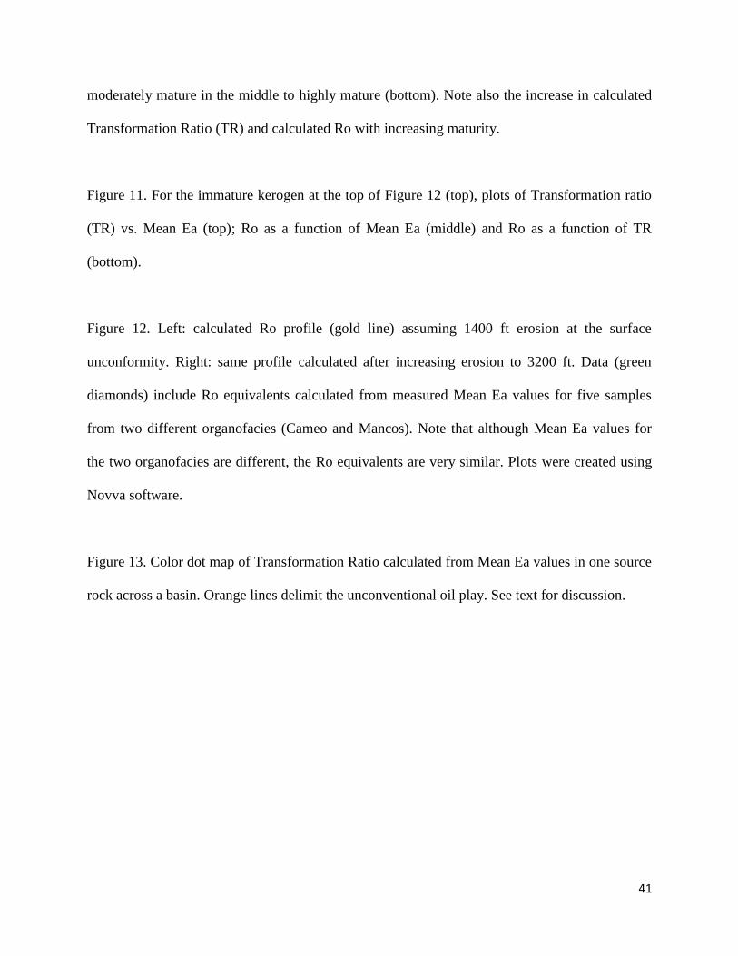
Source-rock kinetics have also been used to aid in sequence-stratigraphic interpretation. Both the
Mean Ea values and the shapes of the Ea distributions within the “F” Member of the
Cenomanian-Santonian Abu Roash Formation of the Western Desert of Egypt can be used to
distinguish different organofacies (Fig. 7). These differences also correlate well with other basic
source-rock parameters (e.g., TOC, Rock-Eval®
S2, Hydrogen Index). The combination of these
various types of data shows that the “F” Member (duration about 2 million years) represents a
single sequence, and delineates the different system tracts within that sequence (Fig. 8).
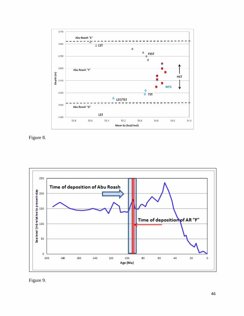
In fact, deposition of the entire Abu Roash Formation and the “F” Member in particular can be
put into the context of global sea-level variation. Figure 9 shows that the Abu Roash was
deposited during a significant event of rising and then falling sea level, and that the “F” Member,
which is the most organic-rich unit in the Abu Roash, was deposited during the highest sea-level
27
stand. That moment provided the deepest water (HST) during all of Abu Roash time, and thus
also gave the best opportunity for development of anoxia and favorable conditions for
preservation of organic matter.
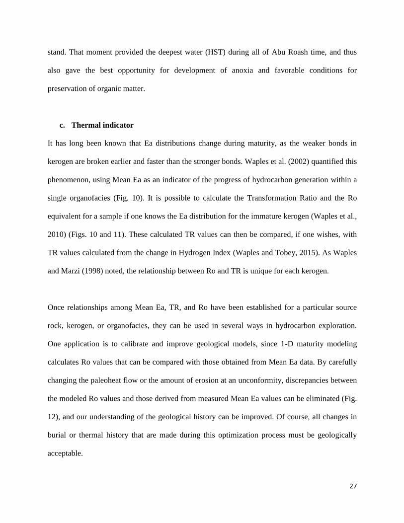
c. Thermal indicator
It has long been known that Ea distributions change during maturity, as the weaker bonds in
kerogen are broken earlier and faster than the stronger bonds. Waples et al. (2002) quantified this
phenomenon, using Mean Ea as an indicator of the progress of hydrocarbon generation within a
single organofacies (Fig. 10). It is possible to calculate the Transformation Ratio and the Ro
equivalent for a sample if one knows the Ea distribution for the immature kerogen (Waples et al.,
2010) (Figs. 10 and 11). These calculated TR values can then be compared, if one wishes, with
TR values calculated from the change in Hydrogen Index (Waples and Tobey, 2015). As Waples
and Marzi (1998) noted, the relationship between Ro and TR is unique for each kerogen.
Once relationships among Mean Ea, TR, and Ro have been established for a particular source
rock, kerogen, or organofacies, they can be used in several ways in hydrocarbon exploration.
One application is to calibrate and improve geological models, since 1-D maturity modeling
calculates Ro values that can be compared with those obtained from Mean Ea data. By carefully
changing the paleoheat flow or the amount of erosion at an unconformity, discrepancies between
the modeled Ro values and those derived from measured Mean Ea values can be eliminated (Fig.
12), and our understanding of the geological history can be improved. Of course, all changes in
burial or thermal history that are made during this optimization process must be geologically
acceptable.

28
Mapping of maturity parameters derived from source-rock kinetics can also be of great value in
exploration. Figure 13 shows a color dot map of Transformation Ratio within one source rock in
numerous wells across a study area. TR was calculated from measured Mean Ea values, which
themselves were obtained at low cost from archived Rock-Eval®
data from a public data
repository, following the approach of Waples et al. (2010). Dot maps are ideal for presenting the
geochemical data in a format that is both scientifically sound and visually impacting.
In this example, it is clear that the TR increases toward the southeast. The orange lines delimit
the user-defined play for unconventional oil, which was established empirically from production
experience, which had previously defined the maximum acceptable GOR (upper TR limit) and
oil viscosity (lower TR limit). Other similar maps such as Ro equivalent or degree of expulsion
could also be used for other purposes in the exploration process, including calibrating regional
thermal history and providing maturity input for migration modeling.
5. Recommendations
Kinetics that describe either total hydrocarbon generation, or generation of oil and gas as two
distinct products, are suitable for the great majority of exploration applications. The quickest and
least-expensive method for determining total-hydrocarbon kinetics is to perform a single open-
system pyrolysis run at a heating rate of about 25oC per minute, to fix the A factor to a
reasonable value (between about 3*1013
s-1
and 8*1014
s-1
) during the derivation of the kinetic
parameters, and to use a spacing of 1 kcal/mole or less in the activation-energy distribution. I do

29
not believe that determination of kinetic parameters using multiple pyrolysis runs is necessary or
desirable.
Separate kinetics for oil generation and gas generation can be estimated, if one wishes. Although
imperfect, this method for dividing total-hydrocarbon kinetics into oil and gas kinetics is
inexpensive and appears to be reliable.
Currently, kinetic parameters for more than two hydrocarbon products must be determined using
completely different technologies. These include open-system-pyrolysis devices coupled to gas
chromatographs, and closed system devices that are either coupled to or independent of gas
chromatographs. Although these compositional-kinetic approaches can be more expensive and
time consuming, they can also yield critical information regarding the relative timing of
generation and the composition of hydrocarbon products. Separate kinetics for multiple
hydrocarbon products are mainly applied where an extremely detailed picture of hydrocarbon
composition is required. Different workers have quite different opinions about the costs and
benefits associated with obtaining this amount of detail.
Utilization of the one-run method for determining kinetics lowers the cost per sample, and thus
permits the acquisition of much larger data bases of source-rock kinetics. These larger data bases
not only provide internal quality control, but also permit the application of source-rock kinetics
in two important new ways: as an indicator of organofacies, and as an indicator of both thermal
history and the progress of hydrocarbon generation. Source-rock kinetics can and should be

30
routinely applied in all three modes in evaluating conventional, unconventional, and hybrid
plays.
In modeling studies decisions about using a single set of kinetics for all products; using different
kinetics for oil and gas; or using one of the various compositional schemes seem to depend very
much on the individual user and on the objectives of each study. A move away from a single set
of kinetics for all products is probably overdue and is now becoming feasible for routine
modeling work.
6. References cited
Behar, F. and M. Vandenbroucke, 1996, Experimental determination of the rate constants of the
n-C25 thermal cracking at 120, 400, and 800 bar: implications for high-pressure/high-
temperature prospects, Energy & Fuels, v. 10, p. 932-940.
Behar, F., S. Kressmann, J.L. Rudkiewicz, and M. Vandenbroucke, 1992, Experimental
simulation in a confined system and kinetic modelling of kerogen and oil cracking, Organic
Geochemistry, v. 19, p. 173–189.
Behar, F., M. Vandenbroucke, Y. Tang, F. Marquis, and J. Espitalié, 1997, Thermal cracking of
kerogen in open and closed systems: Determination of kinetic parameters and stoichiometric
coefficients for oil and gas generation, Organic Geochemistry, v. 26, p. 321– 339.
Benson, S.W., 1976, Thermochemical Kinetics, 2nd edition, New York: John Wiley, 320 p.
Braun R.L. and A.K. Burnham, 1992, PMOD: a flexible model of oil and gas generation,
cracking and expulsion, Lawrence Livermore National Laboratory Report UCRL-JC-105371,
23 p.

31
Braun, R.L. and A.K. Burnham, 1993, Chemical reaction model for oil and gas generation from
Type I and Type II kerogen, Lawrence Livermore National Laboratory Report UCRL-ID-
114143, 26 p.
Braun, R.L., A.K. Burnham, J.G. Reynolds, and J.E. Clarkson, 1991, Pyrolysis kinetics for
lacustrine and marine source rocks by programmed micropyrolysis, Energy & Fuels, v. 5, p.
192-204.
Braun, R.L., A.K. Burnham, and J.G. Reynolds, 1992, Oil and gas evolution kinetics for oil shale
and petroleum source rocks determined from pyrolysis-TQMS data at two heating rates,
Energy & Fuels, v. 6, p. 468-474.
Burnham, A.K., 1994, Comments on "The effects of the mineral matrix on the determination of
kinetic parameters using modified Rock-Eval pyrolysis" by H. Dembicki Jr., and the
resulting comment by R. Pelet, Organic Geochemistry, v. 21, p. 985-986.
Burnham, A.K., 1998, Comment on "Experiments on the role of water in petroleum formation"
by M.D. Lewan, Geochimica et Cosmochimica Acta, v. 62, p. 2207-2210.
Burnham, A.K., R.L. Braun, T.T. Coburn, E.I. Sandvik, D.J. Curry, B.J. Schmidt, and R.A.
Noble, 1996, An appropriate kinetic model for well-preserved algal kerogens, Energy &
Fuels, v. 10, p. 49-59.
Burnham, A. K., A.M. Samoun, and J.G. Reynolds, 1992, Characterization of petroleum source
rocks by pyrolysis-mass spectrometry gas evolution profiles, Lawrence Livermore National
Laboratory Report UCRL-ID-111012, 34 p.
Burrus, J., K. Osadetz, S. Wolf, B. Doligez, K. Visser, and D. Dearborn, 1996, A two-
dimensional regional basin model of Williston Basin hydrocarbon systems, AAPG Bulletin,
v. 80, p. 265-291.

32
Deroo, G., B. Durand, J. Espitalié, R. Pelet, and B. Tissot, 1969, Possibilité d’application des
modèles mathématiques de formation du pétrole à la prospection dans les bassins
sédimentaires, in P.A. Schenck and I. Havenaar (eds.), Advances in Organic Geochemistry
1968, Oxford: Pergamon Press, p. 345-354 (in French).
Dieckmann, V., H.J. Schenk, B. Horsfield, and D.H. Welte, 1998, Kinetics of petroleum
generation and cracking by programmed-temperature closed-system pyrolysis of Toarcian
Shales, Fuel, v. 77, p. 23-31.
Dieckmann, V., B. Horsfield, and H.J. Schenk, 2000, Heating rate dependency of petroleum-
forming reactions: implications for compositional kinetic predictions, Organic Geochemistry,
v. 31, p. 1333-1348.
Di Primio, R. and B. Horsfield, 2006, From petroleum-type organofacies to hydrocarbon phase
prediction, AAPG Bulletin, v. 90, p. 1031-1058.
Dominé, F., 1991, High-pressure pyrolysis of n-hexane, 2,4-dimethylpentane and 1-
phenylbutane. Is pressure an important geochemical parameter? Organic Geochemistry, v.
17, p. 619-634.
Espitalié, J., P. Ungerer, H. Irwin, and F. Marquis, 1988, Primary cracking of kerogens.
Experimenting and modeling C1, C
2-C
5, C
6-C
14 and C
15+ classes of hydrocarbons formed,
Organic Geochemistry, v. 13, p. 893-899.
Higley, D.K. and M.D. Lewan, 2013, Comparison of oil generation kinetics derived from
hydrous pyrolysis and rock-eval in four-dimensional models of the Western Canada
sedimentary basin and its northern Alberta oil sands, in F.J. Hein, D. Leckie, S. Larter, and J.
R. Suter (eds.), Heavy-oil and oil-sand petroleum systems in Alberta and beyond, AAPG
Studies in Geology v. 64, p. 145 – 161.

33
Hoering, T.C., 1984, Thermal reactions of kerogen with added water, heavy water and pure
organic substances, Organic Geochemistry, v. 5, p. 267-278.
Horsfield, B., U. Disko, and F. Leistner, 1989, The micro-scale simulation of maturation: outline
of a new technique and its potential applications, Geologische Rundschau, v. 78, p. 361-373.
Issler, D.R. and L.R. Snowdon, 1990, Hydrocarbon generation kinetics and thermal modelling,
Beaufort-Mackenzie Basin, Bulletin of Canadian Petroleum Geology, v. 38, p. 1-16.
Jüntgen, H. and J. Klein, 1975, Entstehung von Erdgas aus kohligen Sedimenten (Formation of
gas from coaly sediments), Erdöl und Erdgas – Petrochemie vereinigt mit Brennstoff-
Chemie, v. 28, p. 65-73 (in German).
Lakshmanan, C.C., M.L. Bennett, and N. White, 1991, Implications of multiplicity in kinetic
parameters to petroleum exploration: distributed activation energy models, Energy & Fuels,
v. 5, p. 110-117.
Lewan, M.D., 1985, Evaluation of petroleum generation by hydrous pyrolysis experimentation,
Philosophical Transactions of the Royal Society of London. Series A, Mathematical and
Physical Sciences, v. 315, p. 123-134.
Lewan, M.D., 1993, Laboratory simulation of petroleum formation-hydrous pyrolysis, in M.
Engel and S. Macko (eds.), Organic Geochemistry—Principles and Applications, New York:
Plenum Press, p. 419-442.
Lewan, M.D., 1997, Experiments on the role of water in petroleum formation, Geochimica et
Cosmochimica Acta, v. 61, p. 3691-3723.
Lewan, M.D., 1998, Reply to the comment by AK Burnham on "Experiments on the role of
water in petroleum formation", Geochimica et Cosmochimica Acta, v. 62, p. 2211-2216.

34
Lewan, M.D., 2002, New insights on timing of oil and gas generation in the central Gulf Coast
Interior Zone based on hydrous-pyrolysis kinetic parameters, Gulf Coast Association of
Geological Societies Transactions, v. 52, p. 602-620.
Lewan, M.D. and T.E. Ruble, 2002, Comparison of petroleum generation kinetics by isothermal
hydrous and nonisotermal open-system pyrolysis, Organic Geochemistry, v. 33, p. 1457-
1475.
Lewan, M.D., J.C. Winters, and J.H. McDonald, 1979, Generation of oil-like pyrolyzates from
organic-rich shales, Science, v. 203, p. 897-899.
Lopatin, N.V., 1971, Temperatura i geologischeskoe vremya kak faktori uglefikatsii
(Temperature and geologic time as factors in coalification), Izvestiya Akademii Nauk SSSR,
Seriya Geologicheskaya, v. 3, p. 95-106 (in Russian).
Min, W., S.-F. Lu, and H.-T. Xue, 2011, Kinetic simulation of hydrocarbon generation from
lacustrine type I kerogen from the Songliao Basin: Model comparison and geological
application, Marine and Petroleum Geology, v. 28, p. 1714-1726.
Nielsen, S.B. and B. Dahl, 1991, Confidence limits on kinetic models of primary cracking and
implications for the modelling of hydrocarbon generation, Marine and Petroleum Geology, v.
8, p. 489-493.
Nordeng, S.H., 2015, Compensating for the compensation effect using simulated and
experimental kinetics From the Bakken and Red River formations, Williston Basin, North
Dakota, Search and Discovery ***
Pelet, R., 1970, Simulation et modèles mathématiques en geologies, Revue de l’Institut Français
du Pétrole, v. 25, p. 149-164 (in French).
35
Pelet, R., 1985, Sedimentation et evolution geologique de la matiere organique, in B. Labesse,
(ed.), La geologie au service des hommes: Entretiens: Bulletin de la Societe Geologique de
France, Huitieme Serie, v. 1, p. 1075–1086 (in French).
Pepper, A.S. and P.J. Corvi, 1995a, Simple kinetic models of petroleum formation. Part I: oil and
gas generation from kerogen, Marine and Petroleum Geology, v. 12, p. 291-319.
Pepper, A.S. and P.J. Corvi, 1995b, Simple kinetic models of petroleum formation. Part III:
Modelling an open system, Marine and Petroleum Geology, v. 12, p. 417-452.
Peters, K.E., A.K. Burnham, and C.C. Walters, 2015, Petroleum generation kinetics: Single
versus multiple heating-ramp open-system pyrolysis, AAPG Bulletin, v. 99, no. 4, p. 591-
616.
Quigley, T.M. and A.S. Mackenzie, 1988, The temperatures of oil and gas formation in the sub-
surface, Nature, v. 333, p. 549-552.
Ruble, T.E., M.D. Lewan, and R.P. Philp, 2001, New insights on the Green River Petroleum
System in the Uinta Basin from hydrous pyrolysis experiments, AAPG Bulletin, v. 85, p.
1333-1371.
Schenk, H.J. and B. Horsfield, 1993, Kinetics of petroleum generation by programmed-
temperature closed-versus open-system pyrolysis, Geochimica et Cosmochimica Acta, v. 57,
p. 623-630.
Stainforth, J.G., 2009, Practical kinetic modeling of petroleum generation and expulsion, Marine
and Petroleum Geology, v. 26, p. 552-572.
Sundararaman, P., P.H. Merz, and R.G. Mann, 1992, Determination of kerogen activation energy
distribution, Energy & Fuels, v. 6, p. 793-803.
36
Tegelaar, E.W. and R.A. Noble, 1994, Kinetics of hydrocarbon generation as a function of the
molecular structure of kerogen as revealed by pyrolysis-gas chromatography, Organic
Geochemistry, v. 22, p. 543-574.
Tissot, B., 1969, Premières données sur les mécanismes et la cinetique de la formation du pétrole
dans les sédiments. Simulation d’un schéma réactionnel sur ordinateur (First data on the
mechanisms and kinetics of the formation of petroleum in sediments. Simulation of a
reaction scheme on a computer), Revue de l’Institut Français du Pétrole, v. 24, p. 470-501 (in
French).
Tissot, B.P. and J. Espitalié, 1975, L’évolution thermique de la matière organique des sédiments:
applications d’une simulation mathématique (Thermal evolution of sedimentary organic
matter: applications of a mathematical simulation), Revue de l’Institut Français du Pétrole, v.
30, p. 743-777 (in French).
Tissot, B.P., R. Pelet, and Ph. Ungerer, 1987, Thermal history of sedimentary basins, maturation
indices, and kinetics of oil and gas generation, AAPG Bulletin, v. 71, p. 1445-1466.
Ungerer, P., 1984, Models of petroleum formation: how to take into account geology and
chemical kinetics, in B. Durand (ed.), Thermal Phenomena in Sedimentary Basins, Paris:
Editions Technip, p. 235-246.
Ungerer, P. and R. Pelet, 1987, Extrapolation of the kinetics of oil and gas formation from
laboratory to sedimentary basins, Nature, v. 327, p. 52-54.
Ungerer, P., J. Espitalié, F. Marquis, and B. Durand, 1986, Use of kinetic models of organic
matter evolution for the reconstruction of paleotemperatures, in J. Burrus (ed.), Thermal
Modeling in Sedimentary Basins, Paris: Éditions Technip, p. 531-545.

37
Waples, D.W., 1980, Time and temperature in petroleum formation: application of Lopatin's
method to petroleum exploration, AAPG Bulletin, v. 64, p. 916-926.
Waples, D.W., 1984, Thermal models for oil generation, in J.W. Brooks and D.H. Welte (eds.),
Advances in Petroleum Geochemistry, Volume 1, London: Academic Press, p. 7-67.
Waples, D.W., 1996, Comment on "A multicomponent oil-cracking kinetics models for
modeling preservation and composition of reservoired oils" by Lung-Chuan Kuo and G. Eric
Michael, Organic Geochemistry, v. 24, p. 393-395.
Waples, D.W., in press, “Petroleum generation kinetics: Single versus multiple heating-ramp
open-system pyrolysis” by K.E. Peters, A.K. Burnham, and C.C. Walters, AAPG Bulletin, v.
99, no. 4, p. 591-616: Discussion, AAPG Bulletin.
Waples, D.W. and Mahadir Ramly, 2001, A simple way to model non-synchronous generation of
oil and gas from kerogen, Natural Resources Research, v. 10, p. 59-72.
Waples, D.W. and R.W. Marzi, 1998, The universality of the relationship between vitrinite
reflectance and transformation ratio, Organic Geochemistry, v. 28, p. 383-388.
Waples, D. and M. Tobey, 2015, Like space and time, Transformation Ratio is curved, Search
and Discovery ***.
Waples, D.W., A. Vera, and J. Pacheco, 2002, A new method for kinetic analysis of source
rocks: development and application as a thermal and organic facies indicator in the Tithonian
of the Gulf of Campeche, Mexico, Abstracts, 8th Latin American Congress on Organic
Geochemistry, Cartagena, p. 296-298.
Waples, D.W., S. Safwat, R. Nagdy, R. Coskey, and J.E. Leonard, J. E., 2010, A new method for
obtaining personalized kinetics from archived Rock-Eval data, applied to the Bakken

38
Formation, Williston Basin, AAPG International Conference and Exhibition Abstracts
Volume.

39
Figure captions
Figure 1. Logs of A factors shown in histogram form for hydrocarbon-generation kinetics
published for 248 source rocks. All these A factors were determined by allowing both A and Ea
to vary freely during derivation of kinetic parameters from raw pyrolysis data.
Figure 2. Activation-energy distribution for the Mae Sot kerogen from onshore Thailand, with a
spacing of 1 kcal/mole between groups. A = 4.5*1012
s-1
. Data from Tegelaar and Noble, 1994).
Figure 3. Generation of oil and gas from the Type IIb (marine clastic) kerogen published by
Espitalié et al. (1988) using separate oil and gas kinetics at a constant heating rate of 3oC per
million years.
Figure 4. Narrow Ea distribution derived from a homogeneous Type I kerogen (Ordovician-age
Yeoman Formation, Williston Basin, Canada). From Burrus et al. (1996).
Figure 5. Different activation-energy distributions found for kerogens in the Inner Ramp
lithofacies (left) compared to the Outer Ramp lithofacies (right) in the Tithonian of the southern
Gulf of Mexico. A = 1*1014
s-1
for both kerogens. After Waples et al. (2002).
Figure 6. Different activation-energy distributions found for two samples from the same
Ordovician source rock. Left: G. prisca-rich facies with high TOC, with dominant Ea = 55

40
kcal/mole. Right: G. prisca-lean facies with low TOC, with dominant Ea = 54 kcal/mole. A =
1*1014
s-1
for both kerogens.
Figure 7. Ea distributions for three different organofacies identified within the Abu Roash “F”
Member in the northern Western Desert of Egypt. Colors are the same as those used in Figure 8,
where these organofacies are interpreted in a sequence-stratigraphic framework. Values are
Mean Ea in kcal/mol. A = 2*1014
s-1
for all samples. Data courtesy of StratoChem Services.
Figure 8. Sequence stratigraphy of the Abu Roash “F” Member in the northern Western Desert of
Egypt, as interpreted using a variety of source-rock data, including kinetics. All data are from a
single well, and thus maturity levels of all samples are essentially identical – immature. Colors
represent the interpreted system tracts (ST), while symbols represent different shapes of Ea
distributions. L = lowstand; T = transgressive; H = highstand; FS = falling stage; MFS =
maximum flooding surface. Note that Mean Ea values alone would permit correct interpretation
of the sequence stratigraphy. Data courtesy of StratoChem Services.
Figure 9. Relationship between deposition of the Abu Roash Formation, the “F” Member, and
global sea level (blue curve). Sea-level curve courtesy of Michelle Kominz. See text for
discussion.
Figure 10. Activation-energy distributions for three samples from the same organofacies,
showing the change in shape of the Ea distribution as maturity increases from immature (top) to
41
moderately mature in the middle to highly mature (bottom). Note also the increase in calculated
Transformation Ratio (TR) and calculated Ro with increasing maturity.
Figure 11. For the immature kerogen at the top of Figure 12 (top), plots of Transformation ratio
(TR) vs. Mean Ea (top); Ro as a function of Mean Ea (middle) and Ro as a function of TR
(bottom).
Figure 12. Left: calculated Ro profile (gold line) assuming 1400 ft erosion at the surface
unconformity. Right: same profile calculated after increasing erosion to 3200 ft. Data (green
diamonds) include Ro equivalents calculated from measured Mean Ea values for five samples
from two different organofacies (Cameo and Mancos). Note that although Mean Ea values for
the two organofacies are different, the Ro equivalents are very similar. Plots were created using
Novva software.
Figure 13. Color dot map of Transformation Ratio calculated from Mean Ea values in one source
rock across a basin. Orange lines delimit the unconventional oil play. See text for discussion.

42
Figures
Figure 1.
Figure 2.
0
5
10
15
20
25
30
35
40
44 45 46 47 48 49 50 51 52 53 54 55 56
Pe
rce
nt
Activation Energy (kcal/mol)

43
Figure 3.
Figure 4.
0
0.1
0.2
0.3
0.4
0.5
0.6
0.7
0.8
0.9
1
010203040
Frac
tio
n o
f ori
gin
al H
C p
ote
nti
al r
eal
ized
Age (Ma)
Oil
Gas
0
10
20
30
40
50
60
70
80
90
100
50 51 52 53 54 55 56 57 58 59 60
Pe
rce
nt
Ea (kcal/mol)

44
Figure 5.
Figure 6.
Inner Ramp
HI = 635
0
5
10
15
20
25
45 46 47 48 49 50 51 52 53 54 55 56 57 58 59 60 61
Activation Energy (kcal)
Outer Ramp
HI = 691
0
5
10
15
20
25
30
35
40
45
45 46 47 48 49 50 51 52 53 54 55 56 57 58 59 60 61
Activation Energy (kcal)
0
10
20
30
40
50
60
70
80
90
100
39 41 43 45 47 49 51 53 55 57 59 61 63
Rela
tive q
uan
tity
Activation energy (kcal/mole)
0
5
10
15
20
25
30
35
40
45
50
39 41 43 45 47 49 51 53 55 57 59 61 63
Rela
tive q
uan
tity
Activation energy (kcal/mole)

45
Figure 7.
0
2
4
6
8
10
12
14
16
18
20
39 41 43 45 47 49 51 53 55 57 59 61 63
RA
TE
OF
RE
AC
TIO
N
ACTIVATION ENERGY (kcal/mole)A = 2.00E+14/Sec
0
5
10
15
20
25
39 41 43 45 47 49 51 53 55 57 59 61 63
RA
TE
OF
RE
AC
TIO
N
ACTIVATION ENERGY (kcal/mole)A = 2.00E+14/Sec
54.94
54.80
0
5
10
15
20
25
30
39 41 43 45 47 49 51 53 55 57 59 61 63
RA
TE
OF
RE
AC
TIO
N
ACTIVATION ENERGY (kcal/mole)A = 2.00E+14/Sec
55.60
46
Figure 8.
Figure 9.

47
Figure 10.
0
10
20
30
40
50
60
52 53 54 55 56 57 58 59 60 61 62P
erc
en
t
Activation Energy (kcal/mol)
Immature
Mean Ea = 53.80TR = 0
Ro < 0.69
0
10
20
30
40
50
60
52 53 54 55 56 57 58 59 60 61 62
Pe
rce
nt
Activation Energy (kcal/mol)
Early maturity
Mean Ea = 54.12TR = 0.28Ro = 0.85
0
10
20
30
40
50
60
52 53 54 55 56 57 58 59 60 61 62
Pe
rce
nt
Activation Energy (kcal/mol)
High maturity
Mean Ea = 55.54TR = 0.81Ro = 1.11

48
Figure 11.
0
0.2
0.4
0.6
0.8
1
53 54 55 56 57 58 59 60
Cal
cula
ted
TR
Calculated Mean Ea (kcal/mole)
0.2
0.4
0.6
0.8
1.0
1.2
1.4
1.6
1.8
2.0
53 54 55 56 57 58 59 60
Cal
cula
ted
Ro
Calculated Mean Ea (kcal/mole)
0.2
0.4
0.6
0.8
1.0
1.2
1.4
1.6
1.8
2.0
0.0 0.2 0.4 0.6 0.8 1.0
Cal
cula
ted
Ro
Calculated Transformation Ratio

49
Figure 12.
Figure 13.