Sources of carbonaceous aerosols over the United States ...Sources of carbonaceous aerosols over the United States and implications for natural visibility Rokjin J. Park and Daniel

Sources of carbonaceous aerosols over the United States

and implications for natural visibility

Rokjin J. Park and Daniel J. JacobDivision of Engineering and Applied Sciences, Department of Earth and Planetary Sciences, Harvard University, Cambridge,Massachusetts, USA

Mian ChinSchool of Earth and Atmospheric Sciences, Georgia Institute of Technology, Atlanta, Georgia, USA

Randall V. Martin1

Division of Engineering and Applied Sciences, Department of Earth and Planetary Sciences, Harvard University, Cambridge,Massachusetts, USA

Received 18 November 2002; revised 29 January 2003; accepted 12 March 2003; published 20 June 2003.

[1] We use a global three-dimensional model (GEOS-CHEM) to better quantify thesources of elemental carbon (EC) and organic carbon (OC) aerosols in the United Statesthrough simulation of year-round observations for 1998 at a network of 45 sites(Interagency Monitoring of Protected Visual Environments (IMPROVE)). Simulation withour best a priori understanding of sources, including global satellite data to constrain fireemissions, captures most of the variance in the observations (R2 = 0.84 for EC, 0.67for OC) with a low bias of 15% for EC and 26% for OC. Multiple linear regression to fitthe IMPROVE data yields best estimates of 1998 U.S. sources of 0.60 Tg year�1 EC and0.52 Tg year�1 OC from fossil fuel; 0.07 Tg year�1 EC and 0.89 Tg year�1 OCfrom biofuel; 0.08 Tg year�1 EC and 0.60 Tg year�1 OC from wildfires; and1.10 Tg year�1 OC from vegetation. We find that fires in Mexico and Canadacontributed 40–70% of annual mean natural EC in the United States for 1998 and 20–30%of annual mean natural OC. Transpacific transport from Asian pollution sources amountedto less than 10% of the natural EC and less than 2% of the natural OC; in contrast toozone, we find that intercontinental transport of anthropogenic carbonaceous aerosols doesnot enhance significantly the natural background. IMPROVE observations and modelsimulations for the summer of 1995 show that Canadian fire emissions can produce largeevents of elevated EC and OC in the southeastern United States. Our best estimates ofmean natural concentrations of EC and OC in the United States, using a model simulationwith climatological monthly mean fire emissions, are 2–3 times higher than the defaultvalues recommended by the U.S. Environmental Protection Agency for visibilitycalculations, except for OC in the eastern United States (16% lower). INDEX TERMS: 0305

Atmospheric Composition and Structure: Aerosols and particles (0345, 4801); 0345 Atmospheric Composition

and Structure: Pollution—urban and regional (0305); 4801 Oceanography: Biological and Chemical:

Aerosols (0305); KEYWORDS: carbonaceous aerosols, natural visibility, natural aerosol concentrations,

trans-Pacific transport of aerosol, transboundary transport of aerosol, biomass burning aerosol

Citation: Park, R. J., D. J. Jacob, M. Chin, and R. V. Martin, Sources of carbonaceous aerosols over the United States and

implications for natural visibility, J. Geophys. Res., 108(D12), 4355, doi:10.1029/2002JD003190, 2003.

1. Introduction

[2] Carbonaceous aerosol is one of the least understoodcomponents of fine particulate matter (PM). It is usuallydivided in two fractions, elemental carbon (EC) and organiccarbon (OC). OC is the second most abundant component

of the aerosol in the United States after sulfate, and thedominant component of the natural continental aerosol[Malm et al., 2000]. EC is the dominant component of thelight-absorbing aerosol. Carbonaceous aerosol is presentlythe subject of intense scrutiny because of its impact onhuman health, visibility, and climate.[3] We present here an assessment of the sources of EC

and OC in the United States by using a global 3-D model(GEOS-CHEM) simulation of observations from the Inter-agency Monitoring of Protected Visual Environments (IM-PROVE) network. Our focus is on quantifying the

JOURNAL OF GEOPHYSICAL RESEARCH, VOL. 108, NO. D12, 4355, doi:10.1029/2002JD003190, 2003

1Now at Harvard-Smithsonian Center for Astrophysics, Cambridge,Massachusetts, USA.

Copyright 2003 by the American Geophysical Union.0148-0227/03/2002JD003190$09.00

AAC 5 - 1

anthropogenic and natural sources of these aerosols, the roleof transboundary transport, and the implications for visibil-ity. The U.S. Environmental Protection Agency regionalhaze rule [Environmental Protection Agency (EPA), 2001]mandates a schedule of increasing emission controls toachieve ‘‘natural visibility conditions’’ in national parksand other wilderness areas by 2064. The ambiguity indefining ‘‘natural visibility conditions’’ requires better in-formation on natural PM concentrations and the perturbingeffects from fires and from sources outside the UnitedStates.[4] Elemental carbon is emitted to the atmosphere by

combustion. Major sources in the United States include coalburning and diesel engines. Organic carbon is emitteddirectly to the atmosphere (primary OC) and formed in situby condensation of low-volatility products of the photo-oxidation of hydrocarbons (secondary OC). Primary sourcesof OC in the United States are wood fuel, coal burning, andwild fires [Seinfeld and Pandis, 1998; Cabada et al., 2002].Secondary OC includes an anthropogenic component fromoxidation of aromatic hydrocarbons, and a biogenic com-ponent from oxidation of terpenes [Griffin et al., 1999].[5] Our approach is to conduct a 3-D model simulation of

EC and OC concentrations in the United States for 1998,with best a priori sources, compare results with observationsfrom the IMPROVE network, and use the constraints fromthe comparison to optimize our treatment of sources bymultiple linear regression. Our treatment of fire emissionsaccounts for year-to-year variability through satellite obser-vations; 1998 was a particularly active fire year, thusoffering good constraints on emissions from that source.We also present a case study for the summer of 1995 todemonstrate the large-scale enhancements of EC and OCconcentrations in the United States that can arise fromCanadian fires. We go on to quantify mean natural ECand OC concentrations in the United States for differentseasons and regions, using climatological fire emissions andsources from vegetation, and to assess the enhancement ofEC and OC background concentrations resulting fromtranspacific transport of Asian pollution.

2. Model Description

2.1. General

[6] We use the GEOS-CHEM global 3-D model oftropospheric chemistry [Bey et al., 2001] to simulate ECand OC aerosols for 1998 (1 year) and 1995 (summer).The model (version 4.23; see http://www-as.harvard.edu/chemistry/trop/geos/index.html) uses assimilated meteoro-logical data from the NASA Goddard Earth ObservingSystem (GEOS) including winds, convective mass fluxes,mixed layer depths, temperature, precipitation, and surfaceproperties. Meteorological data for 1995 and 1998 areavailable with 6-hour temporal resolution (3-hour forsurface variables and mixing depths), 2� latitude by 2.5�longitude horizontal resolution, and 20 (GEOS1 for 1995)or 48 (GEOS3 for 1998) sigma vertical layers. We retainthis spatial resolution in the GEOS-CHEM simulation. Thelowest model levels are centered at approximately 50, 250,600, 1100, and 1750 m above the local surface in GEOS1and 10, 50, 100, 200, 400, 600, 900, 1200, and 1700 m inGEOS3.

[7] The simulation of carbonaceous aerosols in GEOS-CHEM follows that of the Georgia Tech/Goddard GlobalOzone Chemistry Aerosol Radiation and Transport(GOCART) model [Chin et al., 2002], with a number ofmodifications described below. The model resolves EC andOC, with a hydrophobic and a hydrophilic fraction for each(i.e., four aerosol types). Combustion sources emit hydro-phobic aerosols that then become hydrophilic with ane-folding time of 1.2 days following Cooke et al. [1999]and Chin et al. [2002]. We assume that 80% of EC and 50%of OC emitted from all primary sources are hydrophobic[Cooke et al., 1999; Chin et al., 2002; Chung and Seinfeld,2002]. All secondary OC is assumed to be hydrophilic. Thefour aerosol types in the model are further resolved intocontributions from fossil fuel, biofuel, and biomass burning,plus an OC component of biogenic origin, resulting in atotal of 13 tracers transported by the model.[8] Simulation of aerosol wet and dry deposition follows

the schemes used by Liu et al. [2001] in previous GEOS-CHEM simulations of 210Pb and 7Be aerosol tracers. Wetdeposition includes contributions from scavenging in con-vective updrafts, rainout from convective anvils, and rainoutand washout from large-scale precipitation. Wet depositionis applied only to the hydrophilic component of the aerosol.Dry deposition of aerosols uses a resistance-in-series model[Walcek et al., 1986] dependent on local surface type andmeteorological conditions; it is small compared to wetdeposition. Liu et al. [2001] found no systematic biases intheir simulations of 210Pb and 7Be with GEOS-CHEM.

2.2. A Priori Sources of EC and OC

[9] We use global anthropogenic emissions of EC (6.4 Tgyear�1) and OC (10.5 Tg year�1) from the gridded Cooke etal. [1999] inventory for 1984. This inventory includescontributions from domestic, vehicular, and industrial com-bustion of various fuel types. In the GOCART simulation ofChin et al. [2002], the Cooke et al. [1999] inventory wasused with no seasonal variation. However, the source fromheating fuel should vary with season [Cabada et al., 2002].Cooke et al. [1999] do not resolve the contributions to ECand OC emissions from heating fuel. We assume thesecontributions to represent 8% (EC) and 35% (OC) of totalanthropogenic emissions, based on data for the Pittsburgharea from Cabada et al. [2002] and apply local seasonalvariations of emissions using the heating degree daysapproach [Energy Information Administration (EIA), 1997;Cabada et al., 2002]. In this manner we find that anthro-pogenic EC emission in the United States in winter is 15%higher than in summer. For OC the anthropogenic winteremission is twice that in summer.[10] The Cooke et al. [1999] inventory does not include

biofuels, which provide however an important source ofheating in rural households and are also used in agro-industrial factories. We use a global biofuel use inventorywith 1� � 1� spatial resolution from Yevich and Logan[2003] with emission factors of 1.0 g EC and 5 g OC per drymass burned [Streets et al., 2001; Dickerson et al., 2002].For the United States and Canada, we supersede thatinventory with data on wood fuel consumption for residen-tial and industrial sectors available for individual states andprovinces [EIA, 2001] and which we distribute on a ruralpopulation map. Emission factors for this North American

AAC 5 - 2 PARK ET AL.: CARBONACEOUS AEROSOLS IN THE UNITED STATES

wood fuel source are 0.2 g EC and 3.0 g OC per kg drywood burned [Cabada et al., 2002]. Seasonal variation inbiofuel emissions is included for the United States only andis estimated according to the heating degree-days approach.[11] Biomass burning emissions of EC and OC are

calculated using the global biomass burning inventory ofDuncan et al. [2003]. This inventory uses a fire climatologycompiled on a 1� � 1� grid by Lobert et al. [1999], andapplies monthly and interannual variability to that climatol-ogy from satellite observations. Emission factors are 2g ECand 14 g OC per kg dry mass burned [Chin et al., 2002],higher than for biofuels because combustion is less efficient.For boreal forest fires, which are of particular interest here,emission factors reported in the literature range from 0.38 to2.55 g EC per kg dry mass burned [Lavoue et al., 2000, andreferences therein], consistent with the value assumed here.The OC/EC emission ratio of 7 is within the range of 6.9 to8.2 used by Liousse et al. [1996]. Figure 1 shows theresulting annual OC emissions from biomass burning inNorth and Central America for 1997–2000 as well as theclimatological mean. An ENSO-related drought resulted incatastrophic wildfires in the tropical forests of southernMexico and Central America in 1998 [Peppler et al.,2000]. Canadian fire emissions were also unusually largein 1998. Fire emissions in the United States were 38%higher than the climatological mean.[12] Figure 2 shows the spatial and seasonal distribution

of biomass burning OC emission from our model in 1998.Fires in Mexico and Central America were most intense inMay [Peppler et al., 2000, Cheng and Lin, 2001]. Canadianfires peaked in July–September. In the United States, mostfires occurred in the northwest (Idaho, Montana) in summer;additional fires occurred in spring in Florida, owing to theENSO-induced drought.[13] Secondary formation of OC from oxidation of large

hydrocarbons is an important source but uncertainties arelarge [Griffin et al., 1999; Kanakidou et al., 2000; Chungand Seinfeld, 2002]. Chung and Seinfeld [2002] find that

biogenic terpenes are the main source of secondary OCaerosols. We assume a 10% carbon yield of OC fromterpenes [Chin et al., 2002], and apply this yield to a globalterpene emission inventory dependent on vegetation type,monthly adjusted leaf area index, and temperature [Guentheret al., 1995].[14] Table 1 shows a summary of a priori EC and OC

emissions used in the GEOS-CHEM simulation for 1998.The most important global source for both is biomassburning. In the United States, EC is mostly emitted fromthe combustion of fossil fuel and OC originates mostly fromvegetation (but with large seasonal variation, as discussedbelow).

3. Model Evaluation

[15] A global evaluation of the EC and OC aerosolsimulation was done by Chin et al. [2002] as part of a moregeneral evaluation of aerosol optical depth using ground andsatellite observations. Our simulation of aerosol sources andmeteorological processes is similar to that of Chin et al.[2002] and our global distributions of EC and OC concen-trations are comparable. We focus here our model evaluationon the United States, using observations at the IMPROVEsampling sites. The IMPROVE monitoring program wasinitiated in 1987 in national parks and other protectedenvironments to identify the contribution of different aerosolcomponents to visibility degradation [Malm et al., 1994].

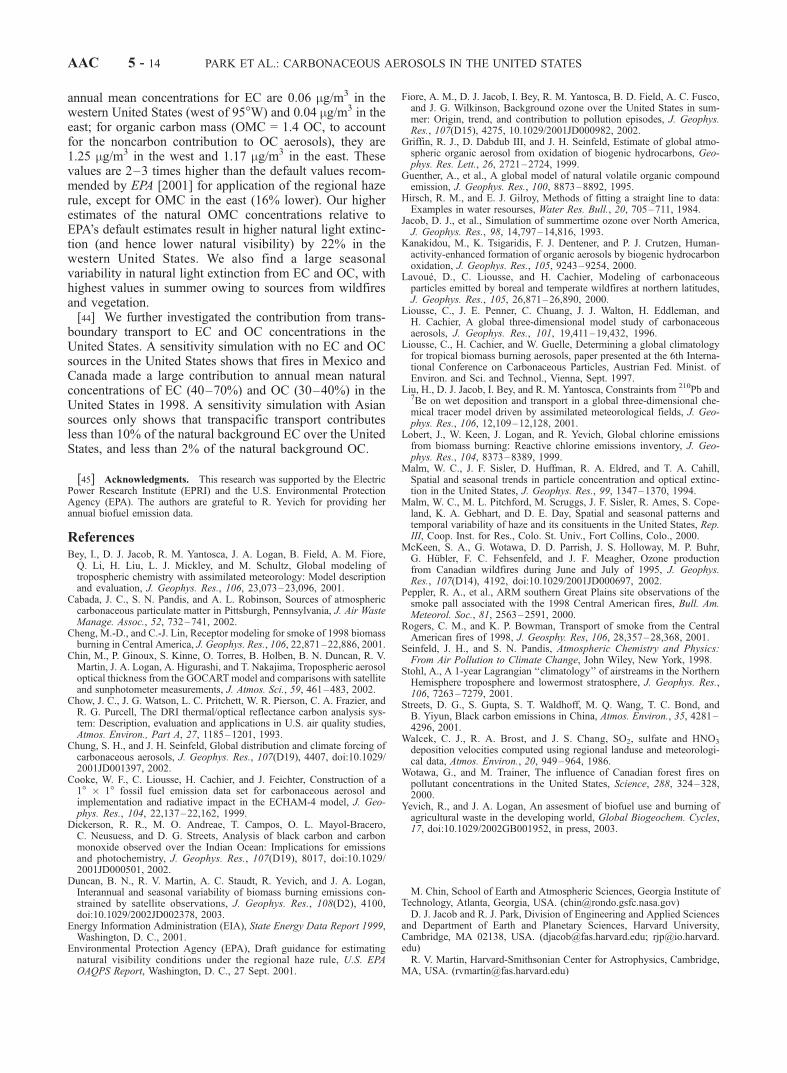
Figure 1. Yearly biomass burning OC emission in 1997–2000 for North and Central America, and climatologicalmean value (see section 2.2).

Figure 2. Annual biomass burning OC emission overNorth and Central America in 1998 (top) and seasonalvariations for different regions (bottom). See color versionof this figure at back of this issue.

PARK ET AL.: CARBONACEOUS AEROSOLS IN THE UNITED STATES AAC 5 - 3

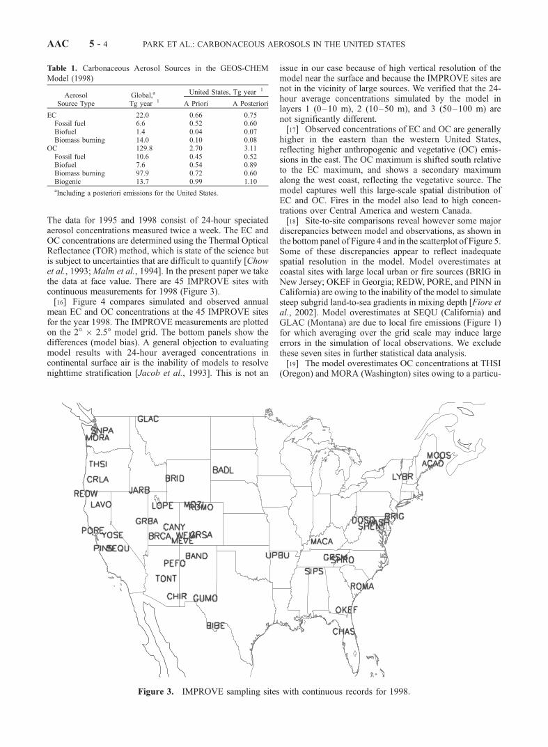
The data for 1995 and 1998 consist of 24-hour speciatedaerosol concentrations measured twice a week. The EC andOC concentrations are determined using the Thermal OpticalReflectance (TOR) method, which is state of the science butis subject to uncertainties that are difficult to quantify [Chowet al., 1993;Malm et al., 1994]. In the present paper we takethe data at face value. There are 45 IMPROVE sites withcontinuous measurements for 1998 (Figure 3).[16] Figure 4 compares simulated and observed annual

mean EC and OC concentrations at the 45 IMPROVE sitesfor the year 1998. The IMPROVE measurements are plottedon the 2� � 2.5� model grid. The bottom panels show thedifferences (model bias). A general objection to evaluatingmodel results with 24-hour averaged concentrations incontinental surface air is the inability of models to resolvenighttime stratification [Jacob et al., 1993]. This is not an

issue in our case because of high vertical resolution of themodel near the surface and because the IMPROVE sites arenot in the vicinity of large sources. We verified that the 24-hour average concentrations simulated by the model inlayers 1 (0–10 m), 2 (10–50 m), and 3 (50–100 m) arenot significantly different.[17] Observed concentrations of EC and OC are generally

higher in the eastern than the western United States,reflecting higher anthropogenic and vegetative (OC) emis-sions in the east. The OC maximum is shifted south relativeto the EC maximum, and shows a secondary maximumalong the west coast, reflecting the vegetative source. Themodel captures well this large-scale spatial distribution ofEC and OC. Fires in the model also lead to high concen-trations over Central America and western Canada.[18] Site-to-site comparisons reveal however some major

discrepancies between model and observations, as shown inthe bottom panel of Figure 4 and in the scatterplot of Figure 5.Some of these discrepancies appear to reflect inadequatespatial resolution in the model. Model overestimates atcoastal sites with large local urban or fire sources (BRIG inNew Jersey; OKEF in Georgia; REDW, PORE, and PINN inCalifornia) are owing to the inability of the model to simulatesteep subgrid land-to-sea gradients in mixing depth [Fiore etal., 2002]. Model overestimates at SEQU (California) andGLAC (Montana) are due to local fire emissions (Figure 1)for which averaging over the grid scale may induce largeerrors in the simulation of local observations. We excludethese seven sites in further statistical data analysis.[19] The model overestimates OC concentrations at THSI

(Oregon) and MORA (Washington) sites owing to a particu-

Table 1. Carbonaceous Aerosol Sources in the GEOS-CHEM

Model (1998)

AerosolSource Type

Global,a

Tg year�1

United States, Tg year�1

A Priori A Posteriori

EC 22.0 0.66 0.75Fossil fuel 6.6 0.52 0.60Biofuel 1.4 0.04 0.07Biomass burning 14.0 0.10 0.08

OC 129.8 2.70 3.11Fossil fuel 10.6 0.45 0.52Biofuel 7.6 0.54 0.89Biomass burning 97.9 0.72 0.60Biogenic 13.7 0.99 1.10aIncluding a posteriori emissions for the United States.

Figure 3. IMPROVE sampling sites with continuous records for 1998.


larly large vegetative source in the model in summer that isapparently not seen in the observations. The discrepancy islocal in nature (it is not found at nearby sites). As discussedfurther below, our specification of the vegetative OC sourceappears inadequate to describe OC concentrations at thesetwo sites, and therefore we exclude them from furtherstatistical analysis.[20] Figure 5 shows that the model generally reproduces

the annual mean EC and OC concentrations to within afactor of two and captures the spatial pattern well (R2 = 0.84

for EC and R2 = 0.67 for OC). However, the slope of thereduced major axis line [Hirsch and Gilroy, 1984] is 0.85 ±0.06 for EC and 0.74 ± 0.08 for OC, reflecting a low bias inthe model. We will correct for this model bias by adjustingthe sources, as discussed below.[21] Figures 6 and 7 compare seasonal variations of

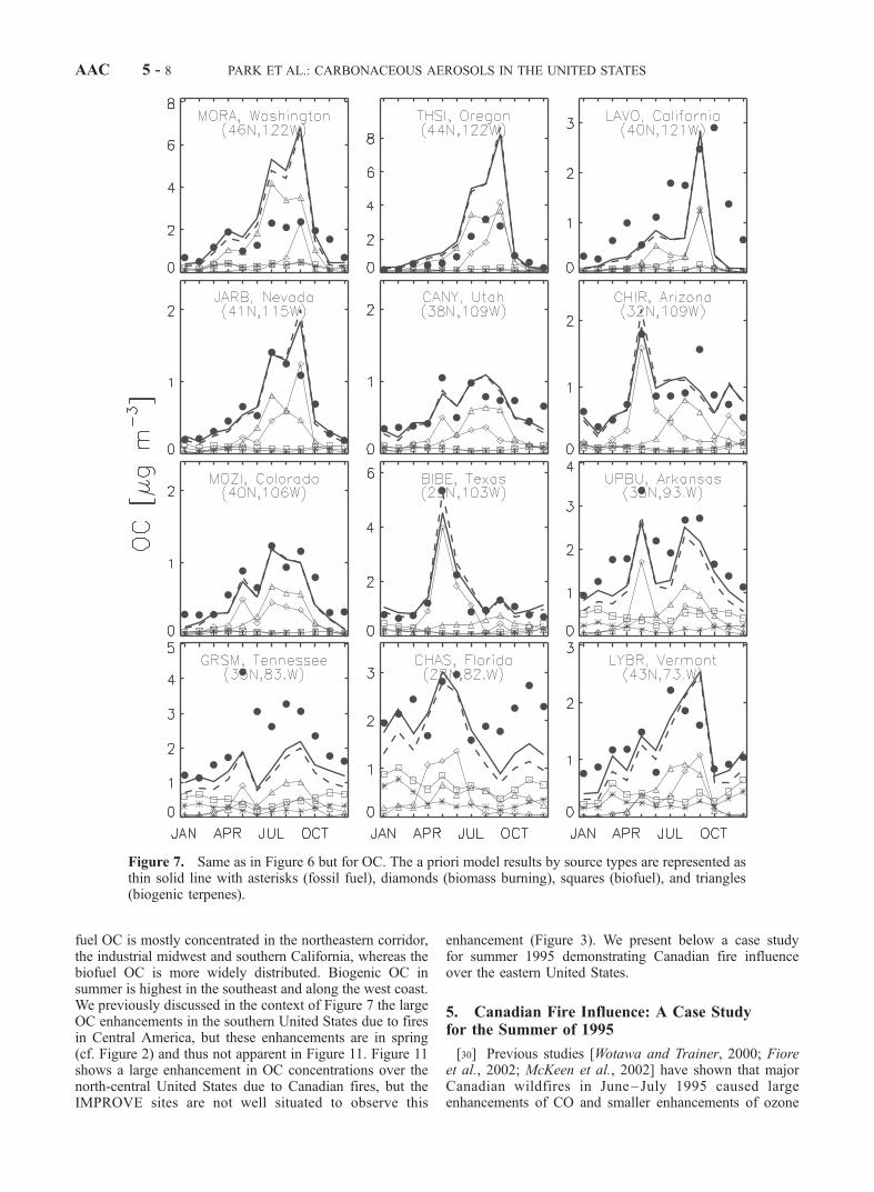
simulated and observed EC and OC concentrations atselected IMPROVE sites. Contributions from individualsources to the model concentrations are shown. Seasonalvariations for EC differ considerably from site to site, and

Figure 4. Annual mean concentrations of EC (left) and OC (right) in surface air over the United Statesin 1998. The top panels show results from the GEOS-CHEM model using a priori sources. The middlepanels shows the IMPROVE observations plotted on the model 2� � 2.5� grid. The bottom panel showsthe difference between the two. See color version of this figure at back of this issue.


the model has significant success in capturing these differ-ences. Fossil fuel is the dominant source for EC at mostsites, but seasonal maxima in May–September over thewestern United States are due to forest fires. The OCconcentrations are generally highest in summer and lowestin winter, both in the model and in the observations; thisseasonal variation is mostly due to the biogenic source.Peaks in OC in May–September in the western UnitedStates are seen both in the model and in the observationsand are due to wildfires, as for EC. Wintertime OC is higherin the eastern than the western United States, and includescontributions of comparable importance from biofuels andfossil fuels.[22] Rogers and Bowman [2001] used satellite measure-

ments and air parcel trajectory calculations to illustrate thetransport of the 1998 fire plumes from Central America tothe central and southern United States. Our model success-

fully captures the corresponding peaks of EC and OCobserved in May at the IMPROVE sites (e.g., BIBE inTexas, CHIR in Arizona, CANY in Utah, MOZI in Colo-rado, UPBU in Arkansas, GRSM in Tennessee). Theenhancement in concentrations is much stronger for OCthan for EC, both in the model and in the observations,reflecting high OC/EC fire emission ratios and the relativelylarge fossil fuel source of EC in the United States.[23] The model has also some success in reproducing the

influences from fire emissions within the United States. Forexample, the high OC in April–June at CHAS in Florida iswell captured in the model. Fires in the western UnitedStates result in peak EC and OC concentrations in Septem-ber at several sites (MORA, Washington; THSI, Oregon;LAVO, California; JARB, Nevada).[24] Figure 8 compares simulated and observed monthly

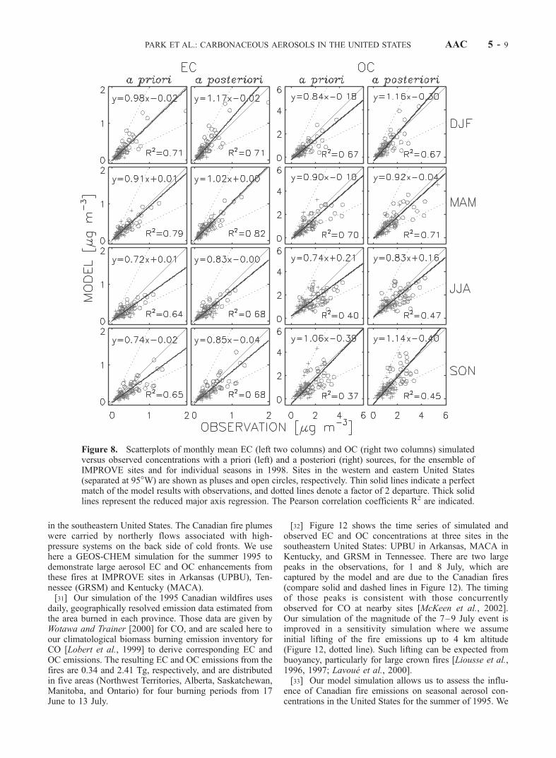
mean concentrations for the ensemble of IMPROVE sitesand for separate seasons. The model simulation with a priorisources has success in reproducing the variability ofobserved EC and OC for winter and spring, as measuredby the high R2 (0.67–0.79) correlation between model andobservations. The slope of the regression line (0.84–0.98) isclose to one for both EC and OC. The R2 is lower insummer and fall, particularly for OC (0.37–0.40) and theslope of the regression line is off from one (0.72–0.74 forEC and 0.74–1.06 for OC). The slope of the OC regressionline in fall is close to one only because high model biasfrom wildfire sources at western sites offsets the low modelbias at eastern sites.

4. Top-Down Emission Estimates

[25] The statistical model biases apparent in Figure8 could reflect errors in the a priori sources. We examinewhat adjustments in the sources would be needed for leastsquares minimization of the bias between simulated andobserved monthly mean EC and OC concentrations. Weidentify for this purpose four source components: fossil fuel,biofuel, biomass burning, and vegetation (the latter for OConly). We use a multiple linear regression to fit the annualmean U.S. source for each component to the monthly meanIMPROVE observations. In order to give equal weight toEC and OC concentrations in the least squares minimiza-tion, we normalize them by their respective annual meanconcentrations for the ensemble of IMPROVE sites (0.29 mgm�3 for EC, 1.23 mg m�3 for OC).[26] We find in this manner that fossil fuel and biofuel

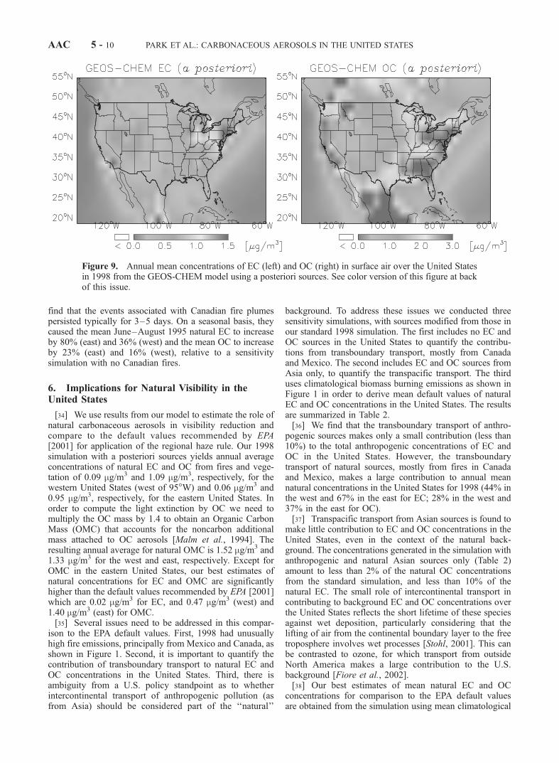
emissions should be increased by 15% and 65% respectivelyfrom a priori levels, while biomass burning emissionsshould be decreased by 17% and the biogenic source forOC should be increased by 11%. We consider these adjust-ments to be well within the uncertainties on the a prioriestimates. The a posteriori values of our adjusted sourcesare given in Table 1. The increase in the biofuel source islargely determined by the model underestimate of observedOC for the cold season.[27] Figure 9 presents annual mean surface air concen-

trations of EC and OC in the model using a posteriorisources. Relative to the simulation with a priori sources(Figure 4), there are 15–20% increases in EC and OCconcentrations in the eastern United States. Changes in thewestern United States are smaller because the decrease in

Figure 5. Scatterplot of simulated (GEOS-CHEM) versusobserved (IMPROVE) annual mean EC and OC concentra-tions for the data shown in Figure 4. The pluses and thecircles indicate data in the western and eastern United States(separated at 95�W), respectively. The asterisks with letterlabels indicate sites discarded in the statistical analysis (seesection 3): REDW(A), PORE(B), PINN(C), SEQU(D),GLAC(E), OKEF(F), and BRIG(G). The squares indicateOC data at MORA(H) and THSI(I) sites which werediscarded in statistical analysis for OC. The thin solid anddotted lines represent the y = x relation and a factor of 2deviation. The thick solid line represents the reduced majoraxis linear regression [Hirsch and Gilroy, 1984], excludingsites A-I. The Pearson correlation coefficients R2 andregression equations are indicated.


the biomass burning source offsets the increase in thebiogenic OC source.[28] The effect of source adjustment on the ability of the

model to fit observed EC and OC concentrations is shownby the scatterplots in Figure 8. Compared to the simulationwith a priori sources, the R2 correlation coefficients areslightly higher and the slopes of the regression lines arecloser to unity. Figures 6 and 7 show the effect of the aposteriori sources on the simulation at individual sites. Theadjustments are generally too small to correct site-specific

discrepancies, which would require modifying the geo-graphic distributions of the sources.[29] Figures 10 and 11 show the contributions of indi-

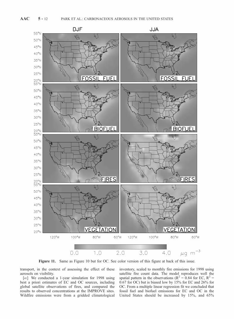
vidual a posteriori sources to EC and OC for winter andsummer. Fossil fuel is the most important source of ECeverywhere in the United States, except in some areas in thewest in summer where wildfires make a more importantcontribution. For OC, the anthropogenic sources (fossil andbiofuel) dominate in winter, while the natural sources (firesand vegetation) are more important in summer. The fossil

Figure 6. Seasonal variation of monthly mean EC concentrations in 1998 at selected IMPROVE sites.Site locations are shown in Figure 1. Values are monthly means. Closed circles indicate the observations.Dashed and solid lines represent the model simulations with a priori and a posteriori sources, respectively.The a priori model components by source types are indicated as thin solid lines with symbols: asterisks(fossil fuel combustion), diamonds (biomass burning), and squares (biofuel use).


fuel OC is mostly concentrated in the northeastern corridor,the industrial midwest and southern California, whereas thebiofuel OC is more widely distributed. Biogenic OC insummer is highest in the southeast and along the west coast.We previously discussed in the context of Figure 7 the largeOC enhancements in the southern United States due to firesin Central America, but these enhancements are in spring(cf. Figure 2) and thus not apparent in Figure 11. Figure 11shows a large enhancement in OC concentrations over thenorth-central United States due to Canadian fires, but theIMPROVE sites are not well situated to observe this

enhancement (Figure 3). We present below a case studyfor summer 1995 demonstrating Canadian fire influenceover the eastern United States.

5. Canadian Fire Influence: A Case Studyfor the Summer of 1995

[30] Previous studies [Wotawa and Trainer, 2000; Fioreet al., 2002; McKeen et al., 2002] have shown that majorCanadian wildfires in June– July 1995 caused largeenhancements of CO and smaller enhancements of ozone

Figure 7. Same as in Figure 6 but for OC. The a priori model results by source types are represented asthin solid line with asterisks (fossil fuel), diamonds (biomass burning), squares (biofuel), and triangles(biogenic terpenes).


in the southeastern United States. The Canadian fire plumeswere carried by northerly flows associated with high-pressure systems on the back side of cold fronts. We usehere a GEOS-CHEM simulation for the summer 1995 todemonstrate large aerosol EC and OC enhancements fromthese fires at IMPROVE sites in Arkansas (UPBU), Ten-nessee (GRSM) and Kentucky (MACA).[31] Our simulation of the 1995 Canadian wildfires uses

daily, geographically resolved emission data estimated fromthe area burned in each province. Those data are given byWotawa and Trainer [2000] for CO, and are scaled here toour climatological biomass burning emission inventory forCO [Lobert et al., 1999] to derive corresponding EC andOC emissions. The resulting EC and OC emissions from thefires are 0.34 and 2.41 Tg, respectively, and are distributedin five areas (Northwest Territories, Alberta, Saskatchewan,Manitoba, and Ontario) for four burning periods from 17June to 13 July.

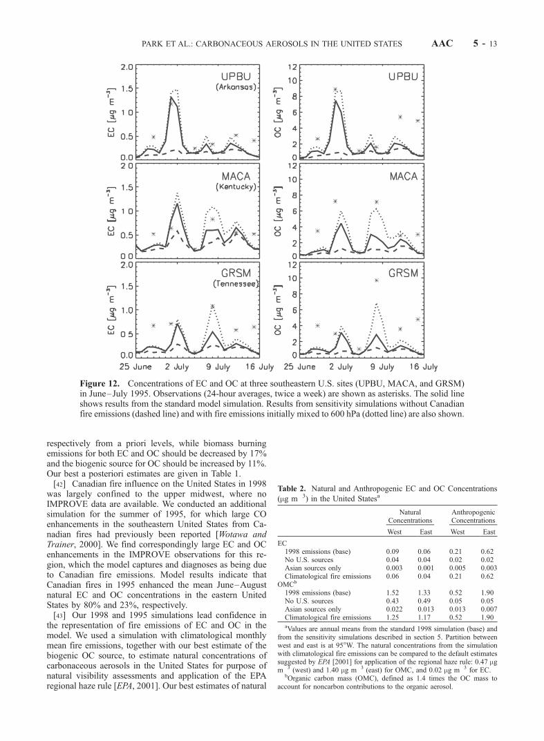
[32] Figure 12 shows the time series of simulated andobserved EC and OC concentrations at three sites in thesoutheastern United States: UPBU in Arkansas, MACA inKentucky, and GRSM in Tennessee. There are two largepeaks in the observations, for 1 and 8 July, which arecaptured by the model and are due to the Canadian fires(compare solid and dashed lines in Figure 12). The timingof those peaks is consistent with those concurrentlyobserved for CO at nearby sites [McKeen et al., 2002].Our simulation of the magnitude of the 7–9 July event isimproved in a sensitivity simulation where we assumeinitial lifting of the fire emissions up to 4 km altitude(Figure 12, dotted line). Such lifting can be expected frombuoyancy, particularly for large crown fires [Liousse et al.,1996, 1997; Lavoue et al., 2000].[33] Our model simulation allows us to assess the influ-

ence of Canadian fire emissions on seasonal aerosol con-centrations in the United States for the summer of 1995. We

Figure 8. Scatterplots of monthly mean EC (left two columns) and OC (right two columns) simulatedversus observed concentrations with a priori (left) and a posteriori (right) sources, for the ensemble ofIMPROVE sites and for individual seasons in 1998. Sites in the western and eastern United States(separated at 95�W) are shown as pluses and open circles, respectively. Thin solid lines indicate a perfectmatch of the model results with observations, and dotted lines denote a factor of 2 departure. Thick solidlines represent the reduced major axis regression. The Pearson correlation coefficients R2 are indicated.


find that the events associated with Canadian fire plumespersisted typically for 3–5 days. On a seasonal basis, theycaused the mean June–August 1995 natural EC to increaseby 80% (east) and 36% (west) and the mean OC to increaseby 23% (east) and 16% (west), relative to a sensitivitysimulation with no Canadian fires.

6. Implications for Natural Visibility in theUnited States

[34] We use results from our model to estimate the role ofnatural carbonaceous aerosols in visibility reduction andcompare to the default values recommended by EPA[2001] for application of the regional haze rule. Our 1998simulation with a posteriori sources yields annual averageconcentrations of natural EC and OC from fires and vege-tation of 0.09 mg/m3 and 1.09 mg/m3, respectively, for thewestern United States (west of 95�W) and 0.06 mg/m3 and0.95 mg/m3, respectively, for the eastern United States. Inorder to compute the light extinction by OC we need tomultiply the OC mass by 1.4 to obtain an Organic CarbonMass (OMC) that accounts for the noncarbon additionalmass attached to OC aerosols [Malm et al., 1994]. Theresulting annual average for natural OMC is 1.52 mg/m3 and1.33 mg/m3 for the west and east, respectively. Except forOMC in the eastern United States, our best estimates ofnatural concentrations for EC and OMC are significantlyhigher than the default values recommended by EPA [2001]which are 0.02 mg/m3 for EC, and 0.47 mg/m3 (west) and1.40 mg/m3 (east) for OMC.[35] Several issues need to be addressed in this compar-

ison to the EPA default values. First, 1998 had unusuallyhigh fire emissions, principally from Mexico and Canada, asshown in Figure 1. Second, it is important to quantify thecontribution of transboundary transport to natural EC andOC concentrations in the United States. Third, there isambiguity from a U.S. policy standpoint as to whetherintercontinental transport of anthropogenic pollution (asfrom Asia) should be considered part of the ‘‘natural’’

background. To address these issues we conducted threesensitivity simulations, with sources modified from those inour standard 1998 simulation. The first includes no EC andOC sources in the United States to quantify the contribu-tions from transboundary transport, mostly from Canadaand Mexico. The second includes EC and OC sources fromAsia only, to quantify the transpacific transport. The thirduses climatological biomass burning emissions as shown inFigure 1 in order to derive mean default values of naturalEC and OC concentrations in the United States. The resultsare summarized in Table 2.[36] We find that the transboundary transport of anthro-

pogenic sources makes only a small contribution (less than10%) to the total anthropogenic concentrations of EC andOC in the United States. However, the transboundarytransport of natural sources, mostly from fires in Canadaand Mexico, makes a large contribution to annual meannatural concentrations in the United States for 1998 (44% inthe west and 67% in the east for EC; 28% in the west and37% in the east for OC).[37] Transpacific transport from Asian sources is found to

make little contribution to EC and OC concentrations in theUnited States, even in the context of the natural back-ground. The concentrations generated in the simulation withanthropogenic and natural Asian sources only (Table 2)amount to less than 2% of the natural OC concentrationsfrom the standard simulation, and less than 10% of thenatural EC. The small role of intercontinental transport incontributing to background EC and OC concentrations overthe United States reflects the short lifetime of these speciesagainst wet deposition, particularly considering that thelifting of air from the continental boundary layer to the freetroposphere involves wet processes [Stohl, 2001]. This canbe contrasted to ozone, for which transport from outsideNorth America makes a large contribution to the U.S.background [Fiore et al., 2002].[38] Our best estimates of mean natural EC and OC

concentrations for comparison to the EPA default valuesare obtained from the simulation using mean climatological

Figure 9. Annual mean concentrations of EC (left) and OC (right) in surface air over the United Statesin 1998 from the GEOS-CHEM model using a posteriori sources. See color version of this figure at backof this issue.


fire emissions. We find annual average concentrations ofnatural EC and OMC of 0.06 mg/m3 and 1.25 mg/m3,respectively, for the western United States and 0.04 mg/m3

and 1.17 mg/m3, respectively, for the eastern United States(Table 2). These are higher by a factor of 2–3 than the EPAdefault values except for OMC in the eastern United Stateswhich is lower by 16%.[39] The implications of our results for natural visibility

estimates are substantial, particularly in the western UnitedStates. Our higher natural OMC component relative toEPA’s default estimates results in lower natural visibility.For example, EPA [2001] uses its default natural PMconcentrations to derive mean light extinctions of 15.60 �10�6 m�1 and 15.78 � 10�6 m�1 at Bandelier NationalMonument (BAND, New Mexico) and at YellowstoneNational Park (YELL, Wyoming). Applying the EPA

[2001] visibility formula with our best estimates of naturalEC and OMC (from the simulation with climatologicalmean fires), and using EPA default values for the otherPM components, we find natural light extinctions of 19.13� 10�6 m�1 and 19.31 � 10�6 m�1 at BAND and YELL,respectively, about 22% higher than EPA values.

7. Conclusions

[40] We used the GEOS-CHEM global 3-D model tosimulate observed concentrations of elemental carbon(EC) and organic carbon (OC) from a network of 45 sitesin relatively remote regions of the United States (IMPROVEnetwork). Our focus was to better quantify the anthropo-genic and natural sources of EC and OC in the UnitedStates, and the role of transboundary and intercontinental

Figure 10. Contribution from different sources types to EC concentrations (mg m�3) in surface air forDJF and JJA. Values are model results for 1998 using a posteriori sources (Table 1). See color version ofthis figure at back of this issue.


transport, in the context of assessing the effect of theseaerosols on visibility.[41] We conducted a 1-year simulation for 1998 using

best a priori estimates of EC and OC sources, includingglobal satellite observations of fires, and compared theresults to observed concentrations at the IMPROVE sites.Wildfire emissions were from a gridded climatological

inventory, scaled to monthly fire emissions for 1998 usingsatellite fire count data. The model reproduces well thespatial pattern in the observations (R2 = 0.84 for EC, R2 =0.67 for OC) but is biased low by 15% for EC and 26% forOC. From a multiple linear regression fit we concluded thatfossil fuel and biofuel emissions for EC and OC in theUnited States should be increased by 15%, and 65%

Figure 11. Same as Figure 10 but for OC. See color version of this figure at back of this issue.


respectively from a priori levels, while biomass burningemissions for both EC and OC should be decreased by 17%and the biogenic source for OC should be increased by 11%.Our best a posteriori estimates are given in Table 1.[42] Canadian fire influence on the United States in 1998

was largely confined to the upper midwest, where noIMPROVE data are available. We conducted an additionalsimulation for the summer of 1995, for which large COenhancements in the southeastern United States from Ca-nadian fires had previously been reported [Wotawa andTrainer, 2000]. We find correspondingly large EC and OCenhancements in the IMPROVE observations for this re-gion, which the model captures and diagnoses as being dueto Canadian fire emissions. Model results indicate thatCanadian fires in 1995 enhanced the mean June–Augustnatural EC and OC concentrations in the eastern UnitedStates by 80% and 23%, respectively.[43] Our 1998 and 1995 simulations lead confidence in

the representation of fire emissions of EC and OC in themodel. We used a simulation with climatological monthlymean fire emissions, together with our best estimate of thebiogenic OC source, to estimate natural concentrations ofcarbonaceous aerosols in the United States for purpose ofnatural visibility assessments and application of the EPAregional haze rule [EPA, 2001]. Our best estimates of natural

Table 2. Natural and Anthropogenic EC and OC Concentrations

(mg m�3) in the United Statesa

NaturalConcentrations

AnthropogenicConcentrations

West East West East

EC1998 emissions (base) 0.09 0.06 0.21 0.62No U.S. sources 0.04 0.04 0.02 0.02Asian sources only 0.003 0.001 0.005 0.003Climatological fire emissions 0.06 0.04 0.21 0.62

OMCb

1998 emissions (base) 1.52 1.33 0.52 1.90No U.S. sources 0.43 0.49 0.05 0.05Asian sources only 0.022 0.013 0.013 0.007Climatological fire emissions 1.25 1.17 0.52 1.90aValues are annual means from the standard 1998 simulation (base) and

from the sensitivity simulations described in section 5. Partition betweenwest and east is at 95�W. The natural concentrations from the simulationwith climatological fire emissions can be compared to the default estimatessuggested by EPA [2001] for application of the regional haze rule: 0.47 mgm�3 (west) and 1.40 mg m�3 (east) for OMC, and 0.02 mg m�3 for EC.

bOrganic carbon mass (OMC), defined as 1.4 times the OC mass toaccount for noncarbon contributions to the organic aerosol.

Figure 12. Concentrations of EC and OC at three southeastern U.S. sites (UPBU, MACA, and GRSM)in June–July 1995. Observations (24-hour averages, twice a week) are shown as asterisks. The solid lineshows results from the standard model simulation. Results from sensitivity simulations without Canadianfire emissions (dashed line) and with fire emissions initially mixed to 600 hPa (dotted line) are also shown.


annual mean concentrations for EC are 0.06 mg/m3 in thewestern United States (west of 95�W) and 0.04 mg/m3 in theeast; for organic carbon mass (OMC = 1.4 OC, to accountfor the noncarbon contribution to OC aerosols), they are1.25 mg/m3 in the west and 1.17 mg/m3 in the east. Thesevalues are 2–3 times higher than the default values recom-mended by EPA [2001] for application of the regional hazerule, except for OMC in the east (16% lower). Our higherestimates of the natural OMC concentrations relative toEPA’s default estimates result in higher natural light extinc-tion (and hence lower natural visibility) by 22% in thewestern United States. We also find a large seasonalvariability in natural light extinction from EC and OC, withhighest values in summer owing to sources from wildfiresand vegetation.[44] We further investigated the contribution from trans-

boundary transport to EC and OC concentrations in theUnited States. A sensitivity simulation with no EC and OCsources in the United States shows that fires in Mexico andCanada made a large contribution to annual mean naturalconcentrations of EC (40–70%) and OC (30–40%) in theUnited States in 1998. A sensitivity simulation with Asiansources only shows that transpacific transport contributesless than 10% of the natural background EC over the UnitedStates, and less than 2% of the natural background OC.

[45] Acknowledgments. This research was supported by the ElectricPower Research Institute (EPRI) and the U.S. Environmental ProtectionAgency (EPA). The authors are grateful to R. Yevich for providing herannual biofuel emission data.

ReferencesBey, I., D. J. Jacob, R. M. Yantosca, J. A. Logan, B. Field, A. M. Fiore,Q. Li, H. Liu, L. J. Mickley, and M. Schultz, Global modeling oftropospheric chemistry with assimilated meteorology: Model descriptionand evaluation, J. Geophys. Res., 106, 23,073–23,096, 2001.

Cabada, J. C., S. N. Pandis, and A. L. Robinson, Sources of atmosphericcarbonaceous particulate matter in Pittsburgh, Pennsylvania, J. Air WasteManage. Assoc., 52, 732–741, 2002.

Cheng, M.-D., and C.-J. Lin, Receptor modeling for smoke of 1998 biomassburning in Central America, J. Geophys. Res., 106, 22,871–22,886, 2001.

Chin, M., P. Ginoux, S. Kinne, O. Torres, B. Holben, B. N. Duncan, R. V.Martin, J. A. Logan, A. Higurashi, and T. Nakajima, Tropospheric aerosoloptical thickness from the GOCARTmodel and comparisons with satelliteand sunphotometer measurements, J. Atmos. Sci., 59, 461–483, 2002.

Chow, J. C., J. G. Watson, L. C. Pritchett, W. R. Pierson, C. A. Frazier, andR. G. Purcell, The DRI thermal/optical reflectance carbon analysis sys-tem: Description, evaluation and applications in U.S. air quality studies,Atmos. Environ., Part A, 27, 1185–1201, 1993.

Chung, S. H., and J. H. Seinfeld, Global distribution and climate forcing ofcarbonaceous aerosols, J. Geophys. Res., 107(D19), 4407, doi:10.1029/2001JD001397, 2002.

Cooke, W. F., C. Liousse, H. Cachier, and J. Feichter, Construction of a1� � 1� fossil fuel emission data set for carbonaceous aerosol andimplementation and radiative impact in the ECHAM-4 model, J. Geo-phys. Res., 104, 22,137–22,162, 1999.

Dickerson, R. R., M. O. Andreae, T. Campos, O. L. Mayol-Bracero,C. Neusuess, and D. G. Streets, Analysis of black carbon and carbonmonoxide observed over the Indian Ocean: Implications for emissionsand photochemistry, J. Geophys. Res., 107(D19), 8017, doi:10.1029/2001JD000501, 2002.

Duncan, B. N., R. V. Martin, A. C. Staudt, R. Yevich, and J. A. Logan,Interannual and seasonal variability of biomass burning emissions con-strained by satellite observations, J. Geophys. Res., 108(D2), 4100,doi:10.1029/2002JD002378, 2003.

Energy Information Administration (EIA), State Energy Data Report 1999,Washington, D. C., 2001.

Environmental Protection Agency (EPA), Draft guidance for estimatingnatural visibility conditions under the regional haze rule, U.S. EPAOAQPS Report, Washington, D. C., 27 Sept. 2001.

Fiore, A. M., D. J. Jacob, I. Bey, R. M. Yantosca, B. D. Field, A. C. Fusco,and J. G. Wilkinson, Background ozone over the United States in sum-mer: Origin, trend, and contribution to pollution episodes, J. Geophys.Res., 107(D15), 4275, 10.1029/2001JD000982, 2002.

Griffin, R. J., D. Dabdub III, and J. H. Seinfeld, Estimate of global atmo-spheric organic aerosol from oxidation of biogenic hydrocarbons, Geo-phys. Res. Lett., 26, 2721–2724, 1999.

Guenther, A., et al., A global model of natural volatile organic compoundemission, J. Geophys. Res., 100, 8873–8892, 1995.

Hirsch, R. M., and E. J. Gilroy, Methods of fitting a straight line to data:Examples in water resourses, Water Res. Bull., 20, 705–711, 1984.

Jacob, D. J., et al., Simulation of summertime ozone over North America,J. Geophys. Res., 98, 14,797–14,816, 1993.

Kanakidou, M., K. Tsigaridis, F. J. Dentener, and P. J. Crutzen, Human-activity-enhanced formation of organic aerosols by biogenic hydrocarbonoxidation, J. Geophys. Res., 105, 9243–9254, 2000.

Lavoue, D., C. Liousse, and H. Cachier, Modeling of carbonaceousparticles emitted by boreal and temperate wildfires at northern latitudes,J. Geophys. Res., 105, 26,871–26,890, 2000.

Liousse, C., J. E. Penner, C. Chuang, J. J. Walton, H. Eddleman, andH. Cachier, A global three-dimensional model study of carbonaceousaerosols, J. Geophys. Res., 101, 19,411–19,432, 1996.

Liousse, C., H. Cachier, and W. Guelle, Determining a global climatologyfor tropical biomass burning aerosols, paper presented at the 6th Interna-tional Conference on Carbonaceous Particles, Austrian Fed. Minist. ofEnviron. and Sci. and Technol., Vienna, Sept. 1997.

Liu, H., D. J. Jacob, I. Bey, and R. M. Yantosca, Constraints from 210Pb and7Be on wet deposition and transport in a global three-dimensional che-mical tracer model driven by assimilated meteorological fields, J. Geo-phys. Res., 106, 12,109–12,128, 2001.

Lobert, J., W. Keen, J. Logan, and R. Yevich, Global chlorine emissionsfrom biomass burning: Reactive chlorine emissions inventory, J. Geo-phys. Res., 104, 8373–8389, 1999.

Malm, W. C., J. F. Sisler, D. Huffman, R. A. Eldred, and T. A. Cahill,Spatial and seasonal trends in particle concentration and optical extinc-tion in the United States, J. Geophys. Res., 99, 1347–1370, 1994.

Malm, W. C., M. L. Pitchford, M. Scruggs, J. F. Sisler, R. Ames, S. Cope-land, K. A. Gebhart, and D. E. Day, Spatial and seasonal patterns andtemporal variability of haze and its consituents in the United States, Rep.III, Coop. Inst. for Res., Colo. St. Univ., Fort Collins, Colo., 2000.

McKeen, S. A., G. Wotawa, D. D. Parrish, J. S. Holloway, M. P. Buhr,G. Hubler, F. C. Fehsenfeld, and J. F. Meagher, Ozone productionfrom Canadian wildfires during June and July of 1995, J. Geophys.Res., 107(D14), 4192, doi:10.1029/2001JD000697, 2002.

Peppler, R. A., et al., ARM southern Great Plains site observations of thesmoke pall associated with the 1998 Central American fires, Bull. Am.Meteorol. Soc., 81, 2563–2591, 2000.

Rogers, C. M., and K. P. Bowman, Transport of smoke from the CentralAmerican fires of 1998, J. Geosphy. Res, 106, 28,357–28,368, 2001.

Seinfeld, J. H., and S. N. Pandis, Atmospheric Chemistry and Physics:From Air Pollution to Climate Change, John Wiley, New York, 1998.

Stohl, A., A 1-year Lagrangian ‘‘climatology’’ of airstreams in the NorthernHemisphere troposphere and lowermost stratosphere, J. Geophys. Res.,106, 7263–7279, 2001.

Streets, D. G., S. Gupta, S. T. Waldhoff, M. Q. Wang, T. C. Bond, andB. Yiyun, Black carbon emissions in China, Atmos. Environ., 35, 4281–4296, 2001.

Walcek, C. J., R. A. Brost, and J. S. Chang, SO2, sulfate and HNO3

deposition velocities computed using regional landuse and meteorologi-cal data, Atmos. Environ., 20, 949–964, 1986.

Wotawa, G., and M. Trainer, The influence of Canadian forest fires onpollutant concentrations in the United States, Science, 288, 324–328,2000.

Yevich, R., and J. A. Logan, An assesment of biofuel use and burning ofagricultural waste in the developing world, Global Biogeochem. Cycles,17, doi:10.1029/2002GB001952, in press, 2003.

��M. Chin, School of Earth and Atmospheric Sciences, Georgia Institute of

Technology, Atlanta, Georgia, USA. ([email protected])D. J. Jacob and R. J. Park, Division of Engineering and Applied Sciences

and Department of Earth and Planetary Sciences, Harvard University,Cambridge, MA 02138, USA. ([email protected]; [email protected])R. V. Martin, Harvard-Smithsonian Center for Astrophysics, Cambridge,

MA, USA. ([email protected])


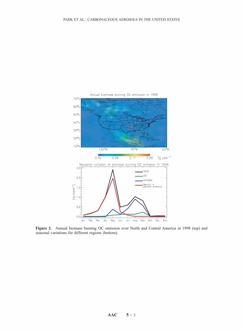
Figure 2. Annual biomass burning OC emission over North and Central America in 1998 (top) andseasonal variations for different regions (bottom).

PARK ET AL.: CARBONACEOUS AEROSOLS IN THE UNITED STATES

AAC 5 - 3

Figure 4. Annual mean concentrations of EC (left) and OC (right) in surface air over the United Statesin 1998. The top panels show results from the GEOS-CHEM model using a priori sources. The middlepanels shows the IMPROVE observations plotted on the model 2� � 2.5� grid. The bottom panel showsthe difference between the two.


AAC 5 - 5

Figure 9. Annual mean concentrations of EC (left) and OC (right) in surface air over the United Statesin 1998 from the GEOS-CHEM model using a posteriori sources.


AAC 5 - 10

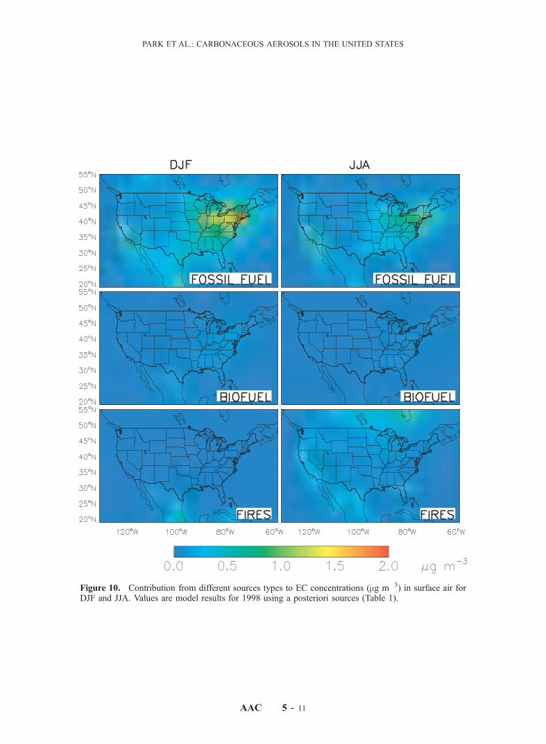
Figure 10. Contribution from different sources types to EC concentrations (mg m�3) in surface air forDJF and JJA. Values are model results for 1998 using a posteriori sources (Table 1).


AAC 5 - 11

Figure 11. Same as Figure 10 but for OC.


AAC 5 - 12

Documents

Sources of carbonaceous aerosols over the United States ...Sources of carbonaceous aerosols over the United States and implications for natural visibility Rokjin J. Park and Daniel