Southern Sierra Nevada wildfire risk assessment: methods …a123.g.akamai.net/7/123/11558/abc123/forestservic... · 2016-05-26 · Southern Sierra Nevada Wildfire Risk Assessment:

Southern Sierra Nevada Wildfire Risk Assessment:

Methods and Results

Prepared by:

Joe Scott - Fire Modeling Specialist, Pyrologix LLC

Julie Gilbertson-Day, Spatial Analyst, Pyrologix LLC

Phil Bowden, Regional Fuels Manager, USDA Forest Service, R5

April Brough, GIS Programmer/Analyst, USDA Forest Service, R5

Don Helmbrecht - Fuels Specialist/Geospatial Analyst, TEAMS Enterprise Unit

Prepared for:

Phil Bowden, Regional Fuels Manager, USDA Forest Service, R5

April 30, 2015

In accordance with Federal civil rights law and U.S. Department of Agriculture (USDA) civil rights regulations and policies, the USDA, its Agencies, offices, and employees, and institutions participating in or administering USDA programs are prohibited from discriminating based on race, color, national origin, religion, sex, gender identity (including gender expression), sexual orientation, disability, age, marital status, family/parental status, income derived from a public assistance program, political beliefs, or reprisal or retaliation for prior civil rights activity, in any program or activity conducted or funded by USDA (not all bases apply to all programs). Remedies and complaint filing deadlines vary by program or incident.

Persons with disabilities who require alternative means of communication for program information (e.g., Braille, large print, audiotape, American Sign Language, etc.) should contact the responsible Agency or USDA’s TARGET Center at (202) 720-2600 (voice and TTY) or contact USDA through the Federal Relay Service at (800) 877-8339. Additionally, program information may be made available in languages other than English.

To file a program discrimination complaint, complete the USDA Program Discrimination Complaint Form, AD-3027, found online at http://www.ascr.usda.gov/complaint_filing_cust.html and at any USDA office or write a letter addressed to USDA and provide in the letter all of the information requested in the form. To request a copy of the complaint form, call (866) 632-9992. Submit your completed form or letter to USDA by: (1) mail: U.S. Department of Agriculture, Office of the Assistant Secretary for Civil Rights, 1400 Independence Avenue, SW, Washington, D.C. 20250-9410; (2) fax: (202) 690-7442; or (3) email: [email protected].

USDA is an equal opportunity provider, employer and lender.

Southern Sierra Nevada Wildfire Risk Assessment: Methods and Results

i

Table of Contents 1. Overview of the Southern Sierra Risk Assessment ..................................................................... 1

1.1 Purpose of the Assessment .................................................................................................... 1 1.2 Analysis area ......................................................................................................................... 1 1.3 Fire Occurrence Areas........................................................................................................... 2

2. Analysis Methods ........................................................................................................................ 4 2.1 Fuelscape ............................................................................................................................... 4 2.2 Historical Wildfire Occurrence ............................................................................................. 5 2.3 Historical Weather ................................................................................................................ 6

2.3.1 FRISK Files .................................................................................................................... 7 2.3.2 FDist Files ...................................................................................................................... 7

2.4 Wildfire Hazard ..................................................................................................................... 7 2.5 HVRA Characterization ........................................................................................................ 9

2.5.1 Human Habitation (WUI) ............................................................................................. 10 2.5.2 Inholdings ..................................................................................................................... 11 2.5.3 Major Infrastructure ...................................................................................................... 11 2.5.4 Recreation and Administrative Infrastructure .............................................................. 11 2.5.5 Visual Resources .......................................................................................................... 12 2.5.6 Critical Terrestrial Habitat ............................................................................................ 12 2.5.7 Timber Resources ......................................................................................................... 12 2.5.8 Watershed Resources .................................................................................................... 12 2.5.9 Vegetation Condition (VCC) ........................................................................................ 13

2.6 Effects Analysis .................................................................................................................. 13 2.7 Risk Source ......................................................................................................................... 14

3. Analysis Results ........................................................................................................................ 14 3.1 Fuelscape ............................................................................................................................. 14

3.1.1 Virtual landscape .......................................................................................................... 14 3.1.2 Vegetation Changes ...................................................................................................... 15 3.1.3 Systematic Method ....................................................................................................... 15 3.1.4 LCP Calibration Workshop .......................................................................................... 15

3.2 Historical Wildfire Occurrence ........................................................................................... 17 3.3 Historical Weather .............................................................................................................. 18 3.4 Wildfire Hazard ................................................................................................................... 19 3.5 HVRA Characterization ...................................................................................................... 25

3.5.1 Human Habitation ........................................................................................................ 25 3.5.2 Inholdings ..................................................................................................................... 27 3.5.3 Major Infrastructure ...................................................................................................... 28 3.5.4 Recreation-Administration Infrastructure ..................................................................... 29 3.5.5 Visual Resources .......................................................................................................... 30 3.5.6.1 Terrestrial Habitat – Northern Spotted Owl .............................................................. 31 3.5.6.2 Terrestrial Habitat – Northern Goshawk ................................................................... 32 3.5.6.3 Terrestrial Habitat – Fisher ........................................................................................ 33 3.5.6.4 Terrestrial Habitat – Sage-grouse .............................................................................. 34 3.5.7 Timber .......................................................................................................................... 35 3.5.8 Watersheds ................................................................................................................... 37 3.5.9 Vegetation Structure ..................................................................................................... 39

3.6 Effects Analysis .................................................................................................................. 40 3.7 Risk-Source ......................................................................................................................... 44

4. References ................................................................................................................................. 47


ii

List of Tables

Table 1. Summary of total area and fire-modeling area in each of the eight fire occurrence areas (FOAs) used in the Southern Sierra Risk Assessment............................................................. 3

Table 2. List of RAWS station used for each fire occurrence area ................................................. 7 Table 3. HVRA identified for the Southern Sierra Wildfire Risk Assessment and associated data

sources. .................................................................................................................................... 9 Table 4. Summary of annual number of fires per million acres, mean size of large fires, and large

fire annual area burned per million acres by FOA. ............................................................... 17 Table 5. Logistic regression coefficients and mean number of large fires per large-fire day. ...... 18 Table 6. Large-fire results summarized by FOA. .......................................................................... 20 Table 7. Response functions for the Human Habitation HVRA. .................................................. 25 Table 8. Response functions for the Inholdings HVRA. ............................................................... 27 Table 9. Response functions for the Major Infrastructure HVRA................................................. 28 Table 10. Response functions for the Inholdings HVRA. ............................................................. 29 Table 11. Response functions for the Visual Resources HVRA. .................................................. 30 Table 12. Response functions for the Terrestrial Habitat – Northern Spotted Owl HVRA .......... 31 Table 13. Response functions for the Terrestrial Habitat – Northern Goshawk HVRA. .............. 32 Table 14. Response functions for the Terrestrial Habitat - Fisher HVRA. ................................... 33 Table 15. Response functions for the Terrestrial Habitat – Sage-grouse HVRA. ......................... 34 Table 16. Response functions for the Timber HVRA. .................................................................. 35 Table 17. Response functions for the Watersheds HVRA. ........................................................... 37 Table 18. Example S-Class transition matrix for the California Montane Jeffrey & Ponderosa Pine

Woodland BpS model............................................................................................................ 39 Table 19. Response function values for fire-caused transitions from one status to another within

an appropriately sized analysis unit for each BpS. ................................................................ 39 Table 20. Listing of 15 BpS classes assessed and their relative importance per unit area. ........... 40


iii

List of Figures

Figure 1. Map of the Southern Sierra Risk Assessment analysis areas. .......................................... 2 Figure 2. Eight fire occurrence areas used in the Southern Sierra Risk Assessment for

summarizing historical fire occurrence. .................................................................................. 3 Figure 3. Map of RAWS stations used in the Southern Sierra Risk Assessment. ........................... 6 Figure 4. Ignition density grids used in the large-fire (left) and lightning only (right) FSim

simulations ............................................................................................................................... 8 Figure 5. ERC(G) by Julian day for each of the four RAWS stations used in fire modeling. ....... 19 Figure 6. Burn probability results for the southern Sierra wildfire risk assessment landscape. .... 21 Figure 7. Conditional flame length probabilities for each of the six flame length classes for the

southern Sierra wildfire risk assessment landscape. .............................................................. 22 Figure 8. Conditional flame length results for the southern Sierra wildfire risk assessment

landscape. .............................................................................................................................. 23 Figure 9. Mean fireline intensity results for the southern Sierra wildfire risk assessment

landscape. .............................................................................................................................. 24 Figure 10. Geospatial distribution of Human Habitation in the southern Sierra wildfire risk

assessment. ............................................................................................................................ 26 Figure 11. Geospatial distribution of Inholdings in the southern Sierra wildfire risk assessment. 27 Figure 12. Geospatial distribution of Major Infrastructure in the southern Sierra wildfire risk

assessment. ............................................................................................................................ 28 Figure 13. Geospatial distribution of Recreation-Administration Infrastructure in the southern

Sierra wildfire risk assessment. ............................................................................................. 29 Figure 14. Geospatial distribution of Visual Resources in the southern Sierra wildfire risk

assessment. ............................................................................................................................ 30 Figure 15. Geospatial distribution of Northern Spotted Owl Habitat in the southern Sierra wildfire

risk assessment. ..................................................................................................................... 31 Figure 16. Geospatial distribution of Northern Goshawk Habitat in the southern Sierra wildfire

risk assessment. ..................................................................................................................... 32 Figure 17. Geospatial distribution of Fisher Habitat in the southern Sierra wildfire risk

assessment. ............................................................................................................................ 33 Figure 18. Geospatial distribution of Sage-grouse Habitat in the southern Sierra wildfire risk

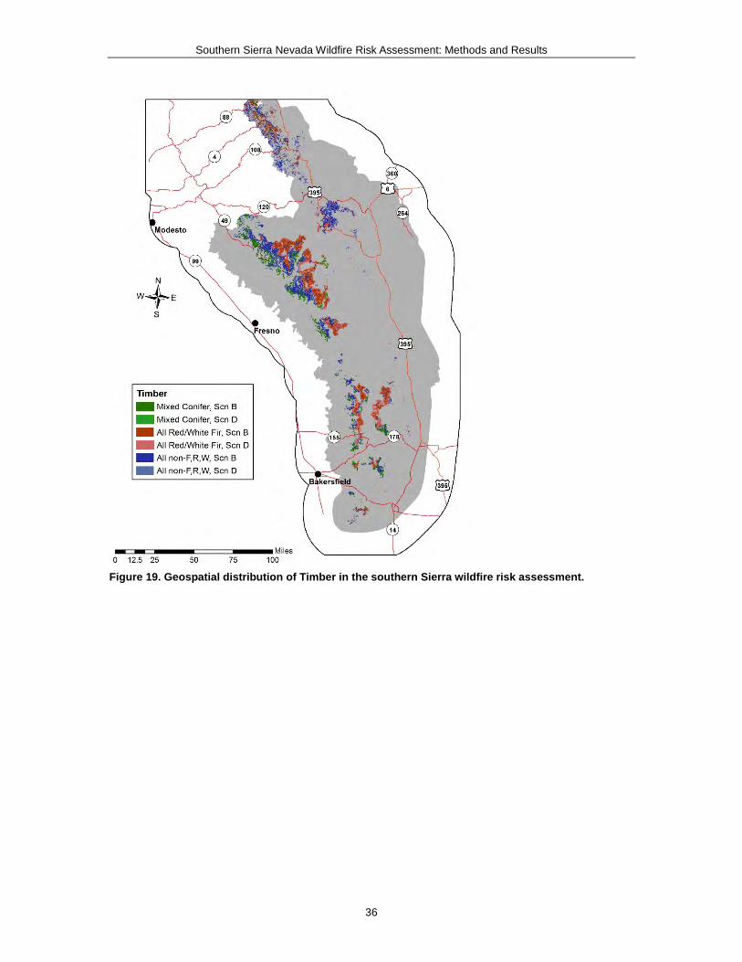
assessment. ............................................................................................................................ 34 Figure 19. Geospatial distribution of Timber in the southern Sierra wildfire risk assessment. ..... 36 Figure 20. Geospatial distribution of Watersheds in the southern Sierra wildfire risk assessment.

............................................................................................................................................... 38 Figure 21. Geospatial distribution of Expected Net Value Change (NVC) for all HVRA in the

southern Sierra wildfire risk assessment. .............................................................................. 42 Figure 22. Geospatial distribution of Conditional Net Value Change (NVC) for all HVRA based

on lightning-only ignitions in the southern Sierra wildfire risk assessment. ......................... 43 Figure 23. Large-fires as a source of NVC. ................................................................................... 45 Figure 24. Lightning fires as a source of NVC.............................................................................. 46


1

1. Overview of the Southern Sierra Risk Assessment 1.1 Purpose of the Assessment The goal of this risk assessment was to provide wildfire risk information and data to the Pacific Southwest Region. This risk information and data is being used by Pacific Southwest Region to aid the Inyo, Sierra, and Sequoia National Forests in their Forest Plan revision efforts.

The main use of the risk assessment is to inform the designations strategic wildfire management areas listed below:

1. Community Wildfire Protection: Identifies the areas with the highest risk to communities and community assets. This could help prioritize fuel treatments by communities.

2. General Wildfire Protection: Identifies the areas with high risk to natural resources and where wildfires often start and threaten communities and as well assets. This could help prioritize fuel treatments and fire management activities.

3. Wildfire Restoration: Identifies the areas with low to moderate risk to mostly natural resources. This could help prioritize ecological restoration projects to create more opportunities under a wider range of conditions to use wildfires to help achieve Forest Plan desired conditions.

4. Wildfire Maintenance: Identifies the areas with very low risk and where wildfires will very likely maintain or help achieve Forest Plan desired conditions. Decision makers should encourage the management of wildfires to meet resource objective whenever possible in this zone.

The risk assessment’s spatial data is useful in analyzing where resource objectives and protection objectives can be met. These strategic areas should support decision makers by providing areas where Wildfire Risk/Potential Benefits have been assessed upfront. Forest Plan guidance organized into these areas also should aid in making wildfire management decisions that meet the full range of Plan objectives.

This risk assessment is anticipated to also be used for fuel treatment planning and prioritization, as well as fire prevention.

1.2 Analysis area The Southern Sierra Risk Assessment analysis area originally encompassed four National Forests: the Inyo, the Sequoia, the Sierra, and the Stanislaus. The fire modeling extent mapped in figure 1 reflects a large buffer around these forests so that valid results could be produced not only within each forest, but also in the land area adjacent to the forests. The Stanislaus National Forest was ultimately dropped from the analysis and the environmental impact statement boundary for Forest Plan revisions was defined which included the Inyo, Sequoia, and Sierra National Forests. All highly valued resources and assets are mapped to the environmental impact statement extent.


2

Figure 1. Map of the Southern Sierra Risk Assessment analysis areas.

1.3 Fire Occurrence Areas The fire modeling area for the Southern Sierra Risk Assessment area is a 24 million acre fire modeling extent characterized by vegetation conditions ranging from valley-bottom grasslands in the Central Valley to alpine timber at the highest elevations, and to arid sagebrush shrubland on the lee side of the Sierra crest. Because this landscape is so large and variable, historical fire occurrence and fire weather summaries for the entire area are inadequate to characterize the variability within and among some of the distinct vegetation communities found along elevation gradients within this landscape. Therefore, we summarized historical fire occurrence for eight different fire occurrence areas within the Southern Sierra Risk Assessment greater landscape. The boundaries for these areas are based on elevation-based ecozones, aggregated where appropriate for fire modeling purposes. The resulting fire occurrence areas are mapped in figure 2 and their land-area extent summarized in table 1.


3

Figure 2. Eight fire occurrence areas used in the Southern Sierra Risk Assessment for summarizing historical fire occurrence.

Table 1. Summary of total area and fire-modeling area in each of the eight fire occurrence areas (FOAs) used in the Southern Sierra Risk Assessment.

Fire Occurrence Areas Total Acres Fire Modeling Acres 1 5,332,359 4,339,750 2 4,043,318 3,103,230 3 2,018,183 2,010,160 4 10,928,467 4,739,260 5 1,442,894 1,034,120 6 2,952,045 2,944,910

7 8,031,384 4,108,740 8 6,438,958 1,746,440


4

2. Analysis Methods 2.1 Fuelscape Spatial fire models need a virtual landscape on which to simulate burning. This virtual landscape is called a fuelscape and is a set of gridded (raster) data layers. The fuelscape consists of data layers representing elevation, slope, aspect, surface fuel model, canopy cover, canopy height, crown base height, and crown bulk density.

For the Southern Sierra Risk Assessment, each grid cell (pixel) represents a square that is 90 meters on a side, representing approximately 2 acres. The Southern Sierra Risk Assessment fuelscape consists of 11,030,199 grid cells representing about 22,060,400 acres, and focused on the three early adopter forests in the Pacific Southwest Region: the Sierra, Sequoia, and Inyo National Forests. This fuelscape size also includes a 10 kilometer buffer around the assessment area so that FSim can simulate fires that ignite outside the assessment but burn into it. These fires need to be modeled because they contribute to the overall wildfire risk inside the assessment area. The fuelscape also covers the Stanislaus National Forest in addition to the early adopter forests.

Prior to conducting a fuelscape calibration workshop, preliminary fire behavior testing using FlamMap5 was completed using a non-calibrated LANDFIRE 2008 (LF_1.1.0) fuelscape. Also much was learned during the Mokelumne Cost Avoidance Analysis (MACA) to identify fuelscape calibration needs on the west side of the central Sierra Nevada.

A calibration workshop involving the region and the early adopter forests was conducted in June 2013 to determine 1) calibration needs and 2) methods to meet those needs and create a fuelscape that best represented current conditions in the Southern Sierra Risk Assessment area.

The following needs were identified and addressed by the region:

• Barren areas in the higher elevation were under represented. Prerelease 2012 data was obtained from LANDFIRE that addressed this known issue in the LANDFIRE 2008 data layers, and incorporated into the calibrated data layers.

• The same general calibrations performed for the west side of the central Sierra Nevada during the Mokelumne Cost Avoidance Analysis were also performed to resolve these calibration needs:

Chaparral shrublands were underrepresented in the area dominated by the LANDFIRE vegetation type of California Blue Oak-Foothill Pine (#2114).

Herbaceous - grassland were under represented in many areas below 4,000 feet elevation.

Agricultural areas below 4,000 feet elevation also seemed under represented.

LANDFIRE vegetation type Red Fir Forest and Woodland (#2032) seemed over represented in areas above 4,000 feet that appeared to be mountain shrublands.

• The Southern Sierra Risk Assessment fuelscape had several zone boundaries that have abrupt changes in fuel characteristics across these boundaries; some of the different fuel characteristics resulted in dramatic differences in modeled fire behavior and needed smoothing to produce a better fuelscape. Existing vegetation type and cover were adjusted by the U.S. Forest Service Fuels Planner using GIS to better calibrate the zone boundary transitions.


5

• The fuelscape needed to have fuel characteristics that best reflect vegetation thru the end 2012, rather than 2008. Updates to the vegetation data layers were made in GIS to ensure recent fires and treatments were included in the calibration process.

• Additionally to the calibration above, the modeled fuel characteristics of many of the vegetation treatments did not reflect the current condition when multiple treatment entries existed. Forests reviewed treatments and provided information describing a more accurate final condition.

• Finally, humid class fuel models were found to not model fuel well and were replaced with similar dry class fuel models.

The LANDFIRE total fuel change for ArcGIS 10 was used to make the final calibrated fuelscape. The LANDFIRE total fuel change uses rule sets for all LANDFIRE vegetation Type (EVT), Cover (EVC), and Height (EVH) and Fuels Disturbance Code (FDIST) combinations to determine Fuel Model assignment. Fuel canopy attributes are calculated by standard Forest Vegetation Simulator/ Fire Fuels Extension4 (FVS/FFE) forest growth simulation model runs by FDIST, EVT, EVH, and EVC combinations. The LFTFC tool performs all calculations at the pixel level, not the stand level.

2.2 Historical Wildfire Occurrence We used the Short (2014) Fire Occurrence Database (FOD) as the foundation for summarizing fire occurrence within each of the eight FOAs described in the previous section. For each FOA, records were selected from the FOD based on the start location of each wildfire. This process produced eight tabular FODs. We retained all attributes of the original FOD, but the main attributes of interest, in addition to the start location, are the start date, final fire size, and cause class (human vs. natural).

These tabular datasets were summarized to estimate two main contemporary, historical large-fire1 occurrence measures for each FOA:

• mean annual number of large fires

• mean annual large-fire area burned

We tabulated these measures across the full extent of the FOA, including portions beyond the fire modeling landscape extent, and normalized the annual occurrence rates to a per-million-acres basis to permit comparison of wildfire occurrence across FOAs.

For each FOA we also generated a pair of “Pyramid charts” that display the contemporary historical wildfire occurrence as a function of final fire size and Julian Day of fire start. One chart in the pair is for lightning-caused wildfires; the other is for human-caused wildfires.

We used the complete FOD to construct a pair of ignition density grids using the kernel density tool in ArcGIS (2 km cell size, 30 km search radius). One grid of the pair was developed for lightning fires of any size; the other was developed for large fires of any cause.

1 A large fire was defined as one reaching at least 247 acres (100 ha) in final size.


6

2.3 Historical Weather After reviewing data available from scores of RAWS stations across the landscape, we ultimately identified four RAWS stations to use for historical fire weather data across the landscape: Blackrock, Oak Creek, Mt. Elizabeth, and Trimmer

These stations are located in relatively representative locations (figure 3) and have a relatively complete and long-duration record of historical weather. Each RAWS was used for one or more fire occurrence areas (table 2).

Figure 3. Map of RAWS stations used in the Southern Sierra Risk Assessment.


7

Table 2. List of RAWS station used for each fire occurrence area Fire Occurrence Areas RAWS Station Used

1 Trimmer 2 Mount Elizabeth 3 Oak Creek 4 Oak Creek 5 Blackrock 6 Blackrock 7 Trimmer 8 Oak Creek

The historical data for each RAWS were used to generate results for use in FSim, including FRISK files and FDist files.

2.3.1 FRISK Files FRISK files were generated for each RAWS using FireFamilyPlus (FFPlus). These files summarize the ERC, dead fuel moisture content, and wind speed and direction data for a RAWS. The FRISK file is used in the FSim simulation system.

2.3.2 FDist Files FDist files (for fire-day distribution) are used by FSim to generate stochastic fire ignitions as a function of ERC. FDist files were generated using an R script that summarizes historical ERC and wildfire occurrence data, performs logistic regression, and then formats the results into the required FDist format.

2.4 Wildfire Hazard For this analysis we used the FSim large-fire simulator to quantify wildfire hazard across the landscape at a pixel size of 180 m (8 acres per pixel). FSim is a comprehensive fire occurrence, growth, behavior, and suppression simulation system that uses locally relevant fuel, weather, topography, and historical fire occurrence information to make a spatially resolved estimate of the contemporary likelihood and intensity of wildfire across the landscape (Finney et al. 2011). Due to the highly varied nature of weather and fire occurrence across the large landscape, we ran FSim for each of the eight fire occurrence areas independently, and then compiled the 8 runs into a single coherent result. For each fire occurrence area, we parameterized and calibrated FSim based on the location of historical fire ignitions within the fire occurrence area, which is consistent with how the historical record is compiled. We then used FSim to start fires only within each fire occurrence area, but allowed those fires to spread outside of the fire occurrence area. This, too, is consistent with how the historical record is compiled.

FSim requires information regarding historical weather. We used the four RAWS identified in the previous section for the necessary weather inputs. Weather data for these RAWS were used to produce monthly distributions of wind speed and direction, season-long trends of mean and standard deviation of Energy Release Component (ERC) for NFDRS fuel model G, and values for 1-, 10-, and 100-h timelag dead fuel moisture content associated with the 80th, 90th and 97th percentile conditions. These inputs are captured in FSim’s FRISK file.


8

FSIM also requires information regarding the contemporary historical occurrence of fire in the analysis area, specifically large fires—those that escape initial attack and require extended suppression response. For each FOA we used the summaries of historical occurrence described above to parameterize and then calibrate FSim.

Historical fire occurrence was not uniform across the fire modeling area—large fires were more likely to occur in some portions of the landscape than others. To account for that spatial non-uniformity, FSim uses a geospatial layer representing the relative ignition density across the landscape. FSim randomly locates wildfires according to this density grid during simulation. As described above, we made two ignition density grids (IDGs) using the Kernel Density tool on ArcGIS for a 2-km cell size and 30-km search radius. One IDG was generated for large fires of any cause class and another for lightning fires of any size (figure 4). Note that these two types of wildland fire occur in very different parts of the landscape.

Figure 4. Ignition density grids used in the large-fire (left) and lightning only (right) FSim simulations

FSim simulations for each fire occurrence area were calibrated to historical measures of large fire occurrence including: mean historical large-fire size, mean annual burn probability, mean annual number of large fires per million acres, and mean annual area burned per million acres. From these measures, two calculations are particularly useful for comparing against and adjusting FSim results: 1) calculations of mean large fire size indicate whether simulated fires need to be larger or smaller on average, and 2) number of large fires per million acres indicates whether FSim has simulated enough fires to match the annual frequency of large fires demonstrated by the historical record.


9

After calibrating FSim for each fire occurrence area independently, the final FSim runs included 10,000 years of simulated fire behavior results including annual burn probability, flame-length probabilities at each of the six flame-length categories, and fire perimeter polygons. We combined the results into a single landscape-wide result where the area-wide burn probability is simply the sum of all eight fire occurrence areas, and flame-length probabilities are weighted by their respective fire occurrence area burn probability and summed across all fire occurrence areas as described in Thompson and others (2013). We then resampled the compiled 180 m results to a 90 m pixel size to match the resolution of the HVRA spatial layers. Using a 90 m fuel model grid, we identified any burnable pixels with zero burn probabilities resulting from the resample to a finer pixel size. To populate these pixels with an appropriate value, we used a moving-window smoothing to calculate the mean burn probability for all burnable pixels on the 90 m landscape, and then used these results to back-fill any remaining burnable pixels with a non-zero burn probability. This same approach was used for both annual burn probability and the six flame length probability grids.

In addition to the large-fire based FSim simulation, we generated fire behavior results for natural ignitions at least 0.1 acres large, based upon lightning-caused ignitions from the historical record. This run differed from the large-fire simulations in that it was run for the entire Southern Sierra Risk Assessment fire modeling extent at a 270 meter pixel size, and fires were allowed to grow uninhibited by FSim’s suppression module for 5,000 iterations. Because naturally ignited fires have not historically been allowed to grow unsuppressed, we could not calibrate our results to historical targets. Instead, we parameterized the simulation with the most relevant information from the large-fire simulations. This included required weather data from the Blackrock RAWS for fuel moisture and ERC(G).

To maintain consistency with the large-fire simulations, pixel-based results were resampled to 90 meters using the same approach as defined above, using a moving-window to calculate appropriate burn probabilities for populating burnable pixels missing a burn probability value.

2.5 HVRA Characterization Prior to use in the risk assessment the location of each HVRA must be depicted spatially to express two key HVRA components: (1) its characteristic wildfire susceptibility and (2) its perceived value. Table 3 lists the HVRA identified for the southern Sierra wildfire risk assessment. The table illustrates the type of spatial datasets we used to depict how the HVRA’s susceptibility and value vary by location. In the following section, a narrative characterization is provided for each HVRA and sub-HVRA.

Table 3. HVRA identified for the Southern Sierra Wildfire Risk Assessment and associated data sources.

HVRA Data Sources

Human habitation (WUI)

Urban core (SNEP Wild Urban Intermix)

Landscan population database

RDPA – Residentially Developed Populated Areas

Digitized forest egress routes

Inholdings

Private land ownership (BLM)


10

Productive timber lands

State Forests

Major infrastructure

Electric power transmission lines

Non-hydroelectric power plants

Communication towers Communication towers/sites

Communication sites (extracted from Rec/Admin datasets)

Hydroelectric power plants

Recreation and administrative infrastructure

FS structures

FS campgrounds NPS building

BLM buildings

Ski areas

Visual resources

Scenic byways

Critical terrestrial habitat

Spotted owl habitat

Goshawk habitat

Fisher habitat

Sage grouse habitat

Habitat maturity (CWHR size/density)

Vegetation lifeform (LANDFIRE vegetation height)

Timber resources

Vegetation (CWHR size/type)

Mechanical Constraints

Watershed resources

Erosion potential

Vegetation lifeform (LANDFIRE vegetation height)

Watershed importance (Forests To Faucets – F2F)

Vegetation condition

VCC – Vegetation Condition Class

2.5.1 Human Habitation (WUI) Human habitation is typically divided into three density groups to reflect the differences in value and susceptibility: high-density, moderate-density, and low-density. These groupings were used as the three sub-HVRAs for this analysis. Given the use of multiple input datasets, the densities for each sub-HVRA are provided below for clarification.

• High-density human habitation

Intermix: Urban Core less than 1 house per 5 acres


11

Intermix: Urban Core greater than or equal to 1 house per 5 acres

Landscan: High density class from Federal Register Guidelines

RDPA: greater than 7.0 people per 7.29 ha (burnable / no burnable)

Egress routes (INF only)

• Moderate-density human habitation

Landscan: Moderate density class from Federal Register Guidelines

RDPA: 0.8-7.0 people per 7.29 ha (burnable / no burnable)

• Low-density human habitation Landscan: Low density class from Federal Register Guidelines

RDPA: 0.01-0.8 people per 7.29 ha (burnable / no burnable)

2.5.2 Inholdings This HVRA focused on the value of non-NFS timber inholdings. Two sub-HVRAs were included to illustrate differences in value and susceptibility: state forests and private timber lands. While the state forest dataset was readily available, private timber owner location data for the state was unfortunately not yet available. In lieu of the anticipated private timber data, identified productive timber lands were overlaid with ownership to model probable private timber locations.

2.5.3 Major Infrastructure Four types of major infrastructure were separated into four sub-HVRAs to reflect varying values and susceptibilities for this HVRA:

• Electric power transmission lines

• Non-hydroelectric power plants

• Communication sites

• Hydroelectric power plants

Communication sites were restricted to the exterior of the human habitation HVRA. Any input data that did not have an area was converted to 180m pixels to better emulate the valued and susceptible area.

2.5.4 Recreation and Administrative Infrastructure This HVRA was divided into two sub-HVRAs based on value. High-developed infrastructure included any sites such as campgrounds, buildings, ski areas, etc. that had a higher value than the low-developed infrastructure, which consisted mainly of toileted sites.

All recreation and administrative infrastructure was restricted to the exterior of the human habitation HVRA. Communication sites were not included in this HVRA, as they were already accounted for in the major infrastructure HVRA.

Any input data that did not have an area were converted to 180m pixels to better emulate the valued and susceptible area.


12

2.5.5 Visual Resources Due to limited available data, scenic byways were the best approximation of valued visual resources in the analysis area. To increase the exposure of the HVRA to wildfire, the centerlines of the scenic byways were buffered ¼ mile. This allows the area around the byway to be included in the analysis to reflect visual value. No data was readily available to reflect variability in susceptibility.

2.5.6 Critical Terrestrial Habitat Four habitat types were identified as valuable for this analysis: owl habitat, goshawk habitat, Fisher habitat, and sage grouse habitat.

The first three habitats (owl, goshawk, fisher) varied in susceptibility according to the maturity of timber. Immature habitat had a timber size of 11-24 inch DBH and >=40% density. Mature habitat had a timber size of >24 inch DBH and >=40% density.

The sage grouse habitat varied in susceptibility (and value) according to the landform, which was derived from existing vegetation height. The susceptibility and value of shrub landforms (representing sagebrush) were differentiated from that of tree landforms (representing pinyon/juniper).

The various combinations of habitat type and maturity/landform generated 8 sub-HVRAs.

2.5.7 Timber Resources Different tree species and sizes of trees respond differently to various wildfire intensities which represents the susceptibility of the timber resource to wildfire. Tree species and size along with terrain steepness and distance from road determined the value of the timber resource.

Three groups of tree species and sizes were identified to reflect different timber values: mixed conifer (1-6 inch DBH), fir (all sizes), and non-fir (greater than 6 inch DBH).

Two sets of operational constraints were used to portray the terrain steepness and distance from road (as well as biological and legal restrictions on timber).

• Scenario B: slope less than 35% and within 1000’ from a road, or slope less than 35% and within 2000’ from a road if timber was greater than 11 inches DBH and greater than 40% density.

• Scenario D: slope less than 50 and within 1000’ from a road, or slope less than 35% and within 2000’ from a road.

The combination of tree type/size and operational constraints resulted in 6 sub-HVRAs.

2.5.8 Watershed Resources The value for this HVRA comes from Forest to Faucets. The variability in susceptibility for watershed resources was spatially assessed using vegetation life form (tree, shrub, grass) and the erosion potential. Erosion potential was modeled using a combination of slope and erosive soils, and could be low, medium, or high. The combination of these datasets generated 27 sub-HVRAs, with varying values and susceptibilities.


13

2.5.9 Vegetation Condition (VCC) Vegetation structure is a key characteristic to which other ecosystem characteristics respond (e.g., natural disturbance regimes, wildlife habitat and connectivity, plant and animal species diversity, and hydrologic regimes) (Helmbrecht 2015). The value and susceptibility of vegetation structure were assessed in this HVRA using biophysical settings, succession class, and relative abundance. Further details can be found in the vegetation condition assessment (VCA) report provided by the TEAMS Enterprise Unit (Helmbrecht 2015). A total of 15 sub-HVRAs, corresponding to the biophysical settings involved, were used in this HVRA.

2.6 Effects Analysis An effects analysis quantifies wildfire risk as the expected value of net response (Finney 2005, Scott and others 2013) also known as expected net value change (eNVC). This approach has previously been applied to a nationwide assessment (Calkin and others 2010) and several forest-level assessments of wildfire risk (Scott and others 2013, Scott and Helmbrecht 2010, Helmbrecht and others 2012). The effects analysis relies on local resource specialists to produce a tabular response function for each HVRA occurring in the analysis area. A response function is a tabulation of the relative change in value of an HVRA if it were to burn in each of six flame-length classes. A positive value in a response function indicates a benefit, or increase in value; a negative value indicates a loss, or decrease in value. Response function values ranged from -100 (greatest possible loss of resource value) to +100 (greatest increase in value).

In order to integrate HVRAs with differing units of measure (for example, habitat vs. homes), relative importance (RI) values were assigned to each HVRA by members of the forest leadership teams for the three Southern Sierra National Forests. Relative importance values were developed by first ranking the HVRAs then assigning an RI value to each. The most important HVRA was assigned RI = 100. Each remaining HVRA was then assigned an RI value indicating its importance relative to that most-important HVRA. Relative Importance rankings for the three forests were combined into a single set of rankings by the fuel planning staff, and then adjusted as needed to ensure consistency within the analysis.

The RI values apply to the overall HVRA on the assessment landscape as a whole. The calculations need to take into account the relative extent of each HVRA to avoid overemphasizing HVRAs that cover many acres. This was accomplished by normalizing the calculations by the relative extent (RE) of each HVRA in the assessment area. Here, relative extent refers to the number of 90-m pixels mapped to each HVRA. In using this method, the relative importance of each HVRA is spread out over the HVRA's extent. An HVRA with few pixels can have a high importance per pixel; and an HVRA with a great many pixels has a low importance per pixel. A weighting factor (WF) representing the relative importance per unit area was calculated for each HVRA.

The RF and WF values were combined with estimates of the flame-length probability (FLP) in each of the six flame-length classes to estimate conditional NVC (cNVC) as the sum-product of flame-length probability (FLP) and response function value (RF) over all the six flame-length classes, with a weighting factor adjustments for the relative importance per unit area of each HVRA, as follows:

𝑐𝑐𝑐𝑐𝑐𝑐𝑐𝑐𝑗𝑗 = �𝐹𝐹𝐹𝐹𝐹𝐹𝑖𝑖 ∗ 𝑅𝑅𝐹𝐹𝑖𝑖𝑗𝑗 ∗ 𝑊𝑊𝐹𝐹𝑗𝑗

𝑛𝑛

𝑖𝑖


14

where i refers to flame length class (n = 6), j refers to each HVRA, WF is the weighting factor based on the relative importance and relative extent (number of pixels) of each HVRA. The cNVC calculation shown above places each pixel of each resource on a common scale (relative importance), allowing them to be summed across all resources to produce the total cNVC at a given pixel.

𝑐𝑐𝑐𝑐𝑐𝑐𝑐𝑐 = �𝑐𝑐𝑐𝑐𝑐𝑐𝑐𝑐𝑗𝑗

𝑚𝑚

𝑗𝑗

where cNVC is calculated for each pixel in the analysis area. Finally, eNVC for each pixel is calculated as the product of cNVC and annual BP:

𝑒𝑒𝑐𝑐𝑐𝑐𝑐𝑐 = 𝑐𝑐𝑐𝑐𝑐𝑐𝑐𝑐 ∗ 𝐵𝐵𝐹𝐹

2.7 Risk Source Identifying the source of risk to HVRAs requires fire perimeter polygons simulated by FSim, as well as the cNVC grid produced from the effects analysis above. Pixel values for cNVC are totaled for all pixels contained by a given fire perimeter. The total NVC for the fire (NVCfire) is calculated as the sum of each pixel (k) that fell within a simulated fire perimeter, as shown in the equation below.

𝑐𝑐𝑐𝑐𝑐𝑐𝑓𝑓𝑖𝑖𝑓𝑓𝑓𝑓 = �𝑐𝑐𝑐𝑐𝑐𝑐𝑐𝑐𝑘𝑘𝑘𝑘

We calculated NVCfire for every fire perimeter on the landscape using the zonal statistics function of the RMRS Raster Utility Tool (USFS 2014) which allows for efficient summation of all pixels contained by a given perimeter (or summary zone), regardless of the other fire perimeters it overlaps. NVCfire is then assigned back to that fire’s ignition location, for every ignition on the landscape to create a point feature layer with NVCfire at each point. The points are then plotted using a smoothing approach to identify the broader trends emerging from 10,000 years of simulated fire data. This exercise was completed for both large fire and lightning-caused simulated fires, and mapped in Figures 24 and 25.

3. Analysis Results The basic wildfire potential results—burn probability, conditional flame length, and mean fireline intensity—are presented for the entire fire modeling area in the sub-section 8.4. Geospatial data regarding additional wildfire potential results are included in the data package. Those datasets include burn probability by flame-length class, Torching Index and Crowning Index.

3.1 Fuelscape

3.1.1 Virtual landscape Spatial fire models need a virtual landscape on which to simulate burning. This virtual landscape is called a fuelscape (LCP) which is a set of gridded (raster) data layers. The LCPs consist of data layers representing elevation, slope, aspect, surface fuel model, canopy cover, canopy height, crown base height, and crown bulk density. On the southern Sierra Nevada LCPs, each grid cell (pixel) represents a square that is 30 meters on a side.


15

3.1.2 Vegetation Changes Vegetation is subject to constant change – and fuels are therefore also dynamic, necessitating a systematic method for reflecting changes spatially so that fire behavior can be accurately accessed.

3.1.3 Systematic Method The LFTFC (LANDFIRE Total Fuel Change) was used as the main method to update and calibrate LCP attributes. The LFTFC tool allows local experts to quickly produce maps that spatially display any proposed fuel characteristics changes. It works through a Microsoft Access database to produce spatial results in ArcMap based on standard LANDFIRE rule sets or ones devised by the user. These rule sets take into account the existing vegetation type (EVT), existing vegetation cover (EVC), existing vegetation height (EVH), and biophysical setting (BpS) from the LANDFIRE grid data. There are also options within LFTFC to add discrete variables in grid format through use of the wildcard option and for subdividing specific areas for different fuel characteristic assignments through the BpS grid. User-defined rule sets made up of EVT, EVC, EVH, and BpS layers, as well as any wildcard selections, are used to change or refine fuels.

3.1.4 LCP Calibration Workshop On June 25 – 27, 2013 wildland fire, fuels and GIS specialists from the Regional Office, the Inyo, the Sierra, the Sequoia and the Stanislaus National Forests met at the Sierra National Forest Supervisor’s Office for a fuelscape calibration workshop. The two goals of this workshop were: 1. Determine calibration needs to correct any problems with the way LANDFIRE version 1.1.0 (circa 2008) fuelscape characterizes fuels and the subsequent modeled fire behavior. 2. Find methods to the calibrate fuelscape to best represent current conditions in the SSRA area.

Following this workshop and previous work on the Mokelumne Watershed Avoided Cost Analysis these Fuelscape calibration needs were identified:

• The LANDFIRE zone lines need to be smoothed out; the SSRA LCP had several zone boundaries that have abrupt changes in fuel characteristics across at these boundaries. Some of the different fuel characteristics result in dramatic differences in modeled fire behavior.

• The LCP needs to have fuel characteristics that best reflect vegetation thru the end 2012.

• The modeled fuel characteristics of many of the vegetation treatments did not reflect the current condition after the multiple treatment entries.

• Barren areas in the higher elevation were under represented.

• Chaparral shrublands were also under represented in the area dominated by the LANDFIRE vegetation type of California Blue Oak-Foothill Pine (#2114).

• Herbaceous - grassland were under represented in many areas below 4,000 feet elevation.

• Agricultural areas below 4,000 feet elevation also seemed under represented. Carrying

• LANDFIRE vegetation type Red Fir Forest and Woodland (#2032) seemed over represented in areas above 4,000 feet that appeared to be mountain shrublands.

• Replace humid class fuel models with similar dry class fuel models.

During FlamMap5 LCP tests and field trips to the project area for Mokelumne Watershed Avoided Cost Analysis using the “out of the box” LANDFIRE versions 1.1.0 LCP the following calibration needs were identified


16

For the base LANDFIRE vegetation data:

1. Barren areas in the higher elevation were under represented.

2. Chaparral shrublands were also under represented in the area dominated by the LANDFIRE vegetation type of California Blue Oak-Foothill Pine (#2114).

3. Herbaceous - grassland were under represented in many areas below 4,000 feet elevation.

4. Agricultural areas below 4,000 feet elevation also seemed under represented.

5. LANDFIRE vegetation type Red Fir Forest and Woodland (#2032) seemed over represented in areas above 4,000 feet that appeared to be mountain shrublands.

An expert opinion crosswalk between CALVEG2 and LANDFIRE Existing Vegetation Type (EVT) was developed by USFS Fuels Planner - Phil Bowden and USFS Fire Ecologist - Neil Sugihara to make the above listed adjustments to the LANDFIRE Vegetation data files.

GIS was used to make the crosswalk adjustments to LANDFIRE vegetation Type (EVT), Cover (EVC), and Height (EVH) raster files.

These raster files were then used in the 0.12 version of the LFTFC (LANDFIRE Total Fuel Change) Tool for ArcGIS 10 to make the required calibrated LCP.

These final calibration raster files were completed for both LANDFIRE versions 1.1.0 and 1.0.5.

Because version 1.1.0 has some imbedded vegetation changes (2001 -2008), the calibrated LANDFIRE version 1.0.5 (circa 2001) was used to bring both baseline and treatment scenario LCPs forward to the baseline year of 2008 using the LFTFC tool. This method avoided modeling a disturbance on vegetation data that already had been changed. The baseline scenario used the

2001- 2008 LANDFIRE Fuel Disturbance grid (FDIST) with the addition of a custom FDIST code applied only to Working Forest treatments.

The project-specific calibrated LANDFIRE version 1.1.0 (circa 2008) was used by other modeling specialists that needed 2008 baseline vegetation information as part of our project, but was not used for fire modeling.

Spatial fire models need a virtual landscape on which to simulate burning. This virtual landscape—called a fuelscape (LCP) which is a set of gridded (raster) data layers. For the SSRA each grid cell (pixel) represents a square that is 90 meters on a side, representing approximately 2 acres. The SSRA LCPs consist of 11,030,199 grid cells representing about 22,060,400 acres. This LCP size includes a 10 kilometer buffer around the assessment area so that FSim can simulate fires that ignite outside the assessment but burn into it. These fires need to be modeled because they contribute to the overall wildfire risk inside the assessment area. The LCP also covers the Stanislaus National Forest besides the early adopter forests. The final LCP has disturbances imbedded in it thru 2012 plus the addition of the Aspen and Carsten fires that occurred on the Sierra National Forest in the late spring/early summer of 2013.

Before the calibration workshop preliminary fire behavior testing using FlamMap5 was completed using a non-calibrated LANDFIRE 2008 (LF_1.1.0) LCP. Also much was learned during the Mokelumne Cost Avoidance Analysis (MACA) to identify LCP calibration needs on the west side of the central Sierra Nevada.


17

The results of our test runs were presented to the MACA Technical Committee and their feedback and a subsequent field trip to the project area helped identify the following calibration needs for the base LANDFIRE vegetation data:

1. Barren areas in the higher elevation were under represented.

2. Chaparral shrublands were also under represented in the area dominated by the LANDFIRE vegetation type of California Blue Oak-Foothill Pine (#2114).

3. Herbaceous - grassland were under represented in many areas below 4,000 feet elevation.

4. Agricultural areas below 4,000 feet elevation also seemed under represented.

5. LANDFIRE vegetation type Red Fir Forest and Woodland (#2032) seemed over represented in areas above 4,000 feet that appeared to be mountain shrublands.

The LANDFIRE Total Fuel Change (LFTFC) 0.12 version for ArcGIS 10 was used to make the needed calibrated LCP. LFTFC uses rule sets for all LANDFIRE vegetation Type (EVT), Cover (EVC), and Height (EVH) and Fuels Disturbance Code (FDIST) combinations to determine Fuel Model assignment. Fuel canopy attributes are calculated by standard Forest Vegetation Simulator/ Fire Fuels Extension4 (FVS/FFE) forest growth simulation model runs by FDIST, EVT, EVH, and EVC combinations. The LFTFC tool performs all calculations at the pixel level, not the stand level.

3.2 Historical Wildfire Occurrence Historical wildfire occurrence varied widely by FOA. Table 4 summarizes the annual number of large fires per million acres, along with mean large-fire size, and annual area burned by large fires per million acres. A general trend of high numbers of large fires and annual area burned for FOAs in the lower elevations is apparent (e.g. FOAs 7, 1, and 2). However, FOAs covering higher elevations and those on the eastern side of the Sierras tend to have fewer fires and typically burn less area annually. FOA 3 is an exception to this trend, with an average fire size of 6,021 acres and 9,212 acres burned annually. Overall, FOA 1 ranks highest in terms of number of fires and annual area burned. FOA 7 ranked second for number of large fires, but on average those fires burned fewer acres (10,264 acres). FOA 4 had the lowest number of large fires (0.92) and burned the least number of acres annually (1,975). Table 3 clearly illustrates the need for distinct FOAs for fire modeling in diverse geographic areas with highly variable fire histories.

Table 4. Summary of annual number of fires per million acres, mean size of large fires, and large fire annual area burned per million acres by FOA.

FOA Annual number of large fires (per million

acres)

Mean large-fire size

Annual area burned (per

million acres) 1 5.89 2,495 14,696 2 3.09 3,417 10,559 3 1.53 6,021 9,212 4 0.92 2,147 1,975 5 2.31 1,902 4,394 6 1.42 2,282 3,240 7 4.48 2,291 10,264 8 0.98 4,307 4,221


18

3.3 Historical Weather Our historical weather analysis yields two files used by FSim for simulating historical weather and determining the weather characteristics that produced large fires historically, the FDist and the FRISK files. The FDist file provides FSim with logistic regression coefficients that predict the likelihood of a large fire occurrence based on the historical relationship between large fires and ERC and tabulates the distribution of large fires by large-fire day. A large-fire day is a day when at least one large fire occurred historically. The information contained in the FDist file is summarized by FOA in Table 5. As demonstrated in Table 5, on average the majority of large fires occur on a single day, however, in some FOAs there is a greater chance of having multiple large-fire starts on a single day. FOAs 1, 2, and 8 have the highest likelihood of more than one fire occurring, with average number of large fires per large-fire day of 1.32, 1.15, and 1.13, respectively.

The logistic regression coefficients together describe large-fire day likelihood P(LFD) at a given ERC(G) as follows:

𝐹𝐹(𝐹𝐹𝐹𝐹𝐿𝐿) =1

1 + 𝑒𝑒−𝐵𝐵𝑎𝑎∗−𝐵𝐵𝑏𝑏∗𝐸𝐸𝐸𝐸𝐸𝐸(𝐺𝐺)

where Ba is coefficient a and Bb is coefficient b listed in table 5. In general, coefficient a describes the likelihood of a large fire at the lowest ERCs, and coefficient b determines the relative difference in likelihood of a large fire at lower versus higher ERC values.

Table 5. Logistic regression coefficients and mean number of large fires per large-fire day. FOA Logistic regression

coefficient a Logistic regression

coefficient b Mean number of large fires per

large-fire day 1 -6.406 0.047 1.32

2 -6.526 0.040 1.15

3 -13.091 0.082 1.04

4 -7.342 0.034 1.01

5 -7.478 0.032 1.08

6 -6.769 0.025 1.06

7 -4.545 0.026 1.09

8 -10.359 0.060 1.13

The FRISK file captures and summarizes weather information from the RAWS station. Specifically, ERC values and descriptive statistics for each day of the year are compiled for all years of available record. Using the mean ERC(G) value corresponding to each Julian day of the year, we compare ERC(G) between the four RAWS stations used in the FSim fire modeling (Figure 5). The two stations west of the Sierra crest – Trimmer and Mount Elizabeth – show very similar mean ERC(G) values throughout most of the year. The stations to the east have less seasonal variability, and Oak Creek is on average warmer and dryer than the Blackrock RAWS.

The weather module in FSim uses these daily ERC(G) values together with percentile ERC(G) to simulate thousands of historical weather years. Additionally, wind data described as the joint probability of wind speed and direction are summarized by month in the FRISK file and sampled


19

at random by FSim and combined with ERC(G) data to create thousands of simulated weather scenarios.

Figure 5. ERC(G) by Julian day for each of the four RAWS stations used in fire modeling.

3.4 Wildfire Hazard FSim produced wildfire hazard results for each FOA including burn probability, conditional flame length probability, and mean fireline intensity grids. Additionally, conditional flame length, calculated as a weighted sum of flame length probability and flame-length class midpoint, was calculated for each FOA. The eight FOAs were combined using the calculations described above to produce integrated maps of wildfire hazard for the entire fire modeling area.

Burn probability in the risk assessment area ranges from less than 0.001 (1 in 1,000 odds) to 0.05 (1 in 33.3 odds) at the highest (figure 6). The highest burn probabilities are typically found on the western side of the Sierra crest, predominately in the zone where vegetation transitions from grass and shrub to timber. These results mimic historical patterns of large fires observed in the area. Mean annual burn probability is 0.007 (1 in 142 odds).

Integrated conditional flame-length probabilities are mapped for the assessment area in figure 7 below. These maps indicate the likelihood of flame-lengths at each intensity level and their associated spatial distribution. Grid values range from 0 to 1 in each panel and are mapped with grey for lower probabilities to red for values closer to 1. These values are used in cNVC and eNVC calculations, multiplied by response function values assigned to HVRAs for each FIL.

Conditional flame lengths reflect the weighted average of the conditional probability of fire intensity times the midpoint of the FIL class. This calculation produces one value per pixel that can be easily mapped to display the spatial variability and likelihood of different flame-length values. Values mapped in figure 8 range from under 1 ft. to greater than 12 ft., with a mean of 4.3 ft. Flame lengths are lowest in the valley bottoms and lower elevations where vegetation is typically shorter (i.e. grass and grass/shrub) and along the Sierra crest in the alpine zone where


20

vegetation is shorter and fires tend to burn under very moderate conditions (Figure 8). Flame lengths are greatest in the shrub and timber fuels west of the Sierra crest and in the northeastern shrub fuel models.

Mean fireline intensity for the assessment area is mapped in figure 9. Overall, patterns of fireline intensity mirror those of conditional flame lengths capturing the effects of spread direction and variability in wind speed and direction as well as fuel moisture. Figure 9 displays more of the spatial variability in the areas of higher intensity with upper values ranging from 3,000 to 8,000 kW/m, but seen in conditional flame lengths only as the category greater than 12 ft. Though the potential for much higher fireline intensities exist on this landscape, the mean is 549 kW/m, reflecting the abundance of mid-range intensities seen primarily in the lower elevations, but also interspersed throughout the higher intensity zones as well.

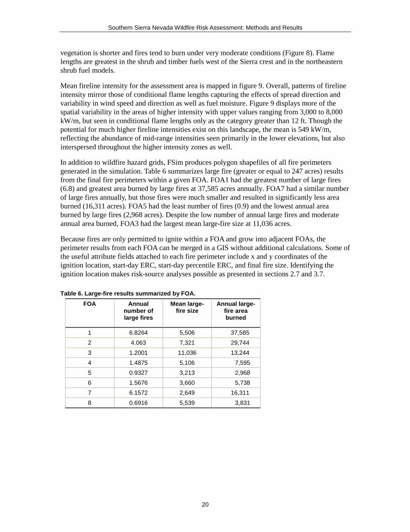
In addition to wildfire hazard grids, FSim produces polygon shapefiles of all fire perimeters generated in the simulation. Table 6 summarizes large fire (greater or equal to 247 acres) results from the final fire perimeters within a given FOA. FOA1 had the greatest number of large fires (6.8) and greatest area burned by large fires at 37,585 acres annually. FOA7 had a similar number of large fires annually, but those fires were much smaller and resulted in significantly less area burned (16,311 acres). FOA5 had the least number of fires (0.9) and the lowest annual area burned by large fires (2,968 acres). Despite the low number of annual large fires and moderate annual area burned, FOA3 had the largest mean large-fire size at 11,036 acres.

Because fires are only permitted to ignite within a FOA and grow into adjacent FOAs, the perimeter results from each FOA can be merged in a GIS without additional calculations. Some of the useful attribute fields attached to each fire perimeter include x and y coordinates of the ignition location, start-day ERC, start-day percentile ERC, and final fire size. Identifying the ignition location makes risk-source analyses possible as presented in sections 2.7 and 3.7.

Table 6. Large-fire results summarized by FOA. FOA Annual

number of large fires

Mean large-fire size

Annual large-fire area burned

1 6.8264 5,506 37,585

2 4.063 7,321 29,744 3 1.2001 11,036 13,244 4 1.4875 5,106 7,595 5 0.9327 3,213 2,968 6 1.5676 3,660 5,738 7 6.1572 2,649 16,311

8 0.6916 5,539 3,831


21

Figure 6. Burn probability results for the southern Sierra wildfire risk assessment landscape.


22

Figure 7. Conditional flame length probabilities for each of the six flame length classes for the southern Sierra wildfire risk assessment landscape.


23

Figure 8. Conditional flame length results for the southern Sierra wildfire risk assessment landscape.


24

Figure 9. Mean fireline intensity results for the southern Sierra wildfire risk assessment landscape.


25

3.5 HVRA Characterization Each HVRA was characterized by one or more data layers of sub-HVRA and, where necessary, further categorized by an appropriate covariate. Covariates include data such as erosion potential categories or age class of habitat (mature versus immature), and population density classes. The main HVRAs in the southern Sierra Wildfire Risk Assessment are mapped below and accompanied by a table with the set of response functions assigned, the within-HVRA relative importance score, and total acres for each sub-HVRA. These components are used along with fire behavior results from FSim in the cNVC and eNVC calculations introduced in section 2.6.

In addition to the HVRAs listed below, the SSRA also assessed the expected effects of wildfire on vegetation structure following the methods described in Scott and others (2014). The TEAMS Enterprise Unit conducted the vegetation condition assessment (VCA) upon which the effects analysis was conducted. Please see the report describing that analysis (Helmbrecht 2015).

3.5.1 Human Habitation We mapped human habitation according to three density classes: low, moderate, and high density. Figure 10 illustrates the distribution of human habitation within the mapped EIS extent. By and large populated pixels follow the major highways in the area, and the higher density classes are predominately located to the west of the Sierra and Sequoia NFs. Response functions shown in table 7 indicate response to fire is overall negative for each density class in all FILs, however, fires in FILs 1-3 are less damaging to high density habitation than in the other two density classes. Relative importance per unit area is greatest for high density human habitation, followed by moderate and low density with weights in proportion to their density classes (table 7).

Table 7. Response functions for the Human Habitation HVRA. Sub-HVRA FIL1 FIL2 FIL3 FIL4 FIL5 FIL6 RI1 Acres

Low density -10 -20 -40 -60 -90 -100 0.05 615,859

Moderate density -10 -20 -40 -60 -90 -100 0.25 475,342

High density -5 -15 -35 -60 -90 -100 1 162,316 1 Within-HVRA relative importance per unit area.


26

Figure 10. Geospatial distribution of Human Habitation in the southern Sierra wildfire risk assessment.


27

3.5.2 Inholdings Inholdings within the NFs representing state and working forests are mapped in figure 11. Private working forests are abundant in the project area, while just one small state forest is mapped. Working forests response to fire is negative for all FILs, while low intensity fire is highly beneficial for state forests, becoming increasingly negative in FILs 3-6 (table 8), and relative importance for state forests is slightly less per unit area at 0.8 than for working forests.

Table 8. Response functions for the Inholdings HVRA. Sub-HVRA FIL1 FIL2 FIL3 FIL4 FIL5 FIL6 RI1 Acres

working forests (private) -10 -40 -60 -80 -80 -80 1 84,255 state forests* 50 70 -10 -50 -70 -100 0.8 5,296

Within-HVRA relative importance per unit area.

Figure 11. Geospatial distribution of Inholdings in the southern Sierra wildfire risk assessment.


28

3.5.3 Major Infrastructure Major infrastructure HVRA consisting of transmission lines, power plants, communication sites, and hydro plants are widely mapped across the EIS extent (figure 12). Transmission lines and communication sites are the most abundant, with fewer pixels of power plants and hydro plants. Response to fire is either neutral in low FILs or slightly negative in the highest FILs. Relative importance shown in table 9 is equivalent for all but transmission lines, which due to their abundant mapped extent, is reduced relative to the other major infrastructure sub-HVRA.

Table 9. Response functions for the Major Infrastructure HVRA Sub-HVRA FIL1 FIL2 FIL3 FIL4 FIL5 FIL6 RI1 Acres

Transmission lines 0 0 0 -10 -20 -40 0.2 207,064

Power Plants 0 0 0 0 -10 -20 1 1,879 Communication Sites 0 0 0 0 -10 -20 1 20,770

Hydro Plant 0 0 0 0 -10 -20 1 376 1 Within-HVRA relative importance per unit area

Figure 12. Geospatial distribution of Major Infrastructure in the southern Sierra wildfire risk assessment.


29

3.5.4 Recreation-Administration Infrastructure Recreation and administration infrastructure is located throughout the study area (figure 13). High-developed infrastructure is prevalent in this landscape and responds negatively to fire in all FILs, increasingly so with increasing intensities (table 10). Low-developed is less common and has a neutral response to fires in FILs 1, and 2 and mildly negative response to fires in FILs 3-6. Low-developed sites have slightly less importance per unit area than high-developed as shown in table 10.

Table 10. Response functions for the Inholdings HVRA. Sub-HVRA FIL1 FIL2 FIL3 FIL4 FIL5 FIL6 RI1 Acres

High Developed -10 -20 -40 -60 -90 -100 1 13,030 Low Developed 0 0 -5 -10 -20 -40 0.67 1,613

1 Within-HVRA relative importance per unit area.

Figure 13. Geospatial distribution of Recreation-Administration Infrastructure in the southern Sierra wildfire risk assessment.


30

3.5.5 Visual Resources Visual resources in the project area consist of scenic byways. These significant roadways are mapped in figure 14, and as shown in table 11, have a highly beneficial response to fires in FIL1 with an increasingly negative response to fires in FILs 2-6. Because it is the only sub-HVRA in the visual resources category, it holds all of the relative importance assigned to the HVRA.

Table 11. Response functions for the Visual Resources HVRA. Sub-HVRA FIL1 FIL2 FIL3 FIL4 FIL5 FIL6 RI1 Acres

Scenic byways 70 -10 -50 -100 -100 -100 1 216,364


Figure 14. Geospatial distribution of Visual Resources in the southern Sierra wildfire risk assessment.


31

3.5.6.1 Terrestrial Habitat – Northern Spotted Owl Northern spotted owl (Strix occidentalis caurina) habitat is abundant primarily in the Sierra and Sequoia NFs. Mature habitat consisting of more mature trees, is less abundant than immature habitat (figure 15), therefore, it has a higher per unit area importance than immature habitat (table 12). Both mature an immature spotted owl habitat respond favorably to fires in FILs 1-3, but negatively to FILs greater than four. Immature habitat shows a greater benefit to fire than mature in FIL1 and FIL2, but also greater loss in FIL5 and FIL6 (table 12).

Table 12. Response functions for the Terrestrial Habitat – Northern Spotted Owl HVRA Sub-HVRA FIL1 FIL2 FIL3 FIL4 FIL5 FIL6 RI1 Acres

Owl, mature 60 80 90 -10 -30 -60 1 287,302

Owl, immature 70 90 90 -10 -50 -80 0.67 581,738 1 Within-HVRA relative importance per unit area.

Figure 15. Geospatial distribution of Northern Spotted Owl Habitat in the southern Sierra wildfire risk assessment.


32

3.5.6.2 Terrestrial Habitat – Northern Goshawk Northern goshawk (Accipiter gentilis atricapillus) habitat is abundant in the Sierra and Sequoia NFs and to a lesser extent in the Inyo NF. Mature habitat is less abundant than immature habitat (figure 16), therefore, it has a higher per unit area importance than immature habitat (table 13). Both mature an immature goshawk habitat types respond favorably to fires in FILs 1-3, but negatively to FILs greater than four. Immature habitat shows a greater benefit to fire than mature in FIL1 and FIL2, but also greater loss in FIL5 and FIL6 (table 13).

Table 13. Response functions for the Terrestrial Habitat – Northern Goshawk HVRA. Sub-HVRA FIL1 FIL2 FIL3 FIL4 FIL5 FIL6 RI1 Acres

Goshawk, mature 60 80 90 -10 -30 -60 1 328,825

Goshawk, immature 70 90 90 -10 -50 -80 0.67 749,478 1 Within-HVRA relative importance per unit area

Figure 16. Geospatial distribution of Northern Goshawk Habitat in the southern Sierra wildfire risk assessment.


33

3.5.6.3 Terrestrial Habitat – Fisher Habitat for the fisher (Martes pennanti) in the project area is mapped in figure 17. Immature habitat is more abundant and therefore has a lower per unit area importance than mature habitat. As with both spotted owl and goshawk habitat, both mature an immature fisher habitat types respond favorably to fires in FILs 1-3, but negatively to FILs greater than four. Immature habitat shows a greater benefit to fire than mature in FIL1 and FIL2, but also greater loss in FIL5 and FIL6 (table 14)

Table 14. Response functions for the Terrestrial Habitat - Fisher HVRA. Sub-HVRA FIL1 FIL2 FIL3 FIL4 FIL5 FIL6 RI1 Acres

Fisher, mature 60 80 90 -10 -30 -60 1 179,273

Fisher, immature 70 90 90 -10 -50 -80 0.67 319,513


Figure 17. Geospatial distribution of Fisher Habitat in the southern Sierra wildfire risk assessment.


34

3.5.6.4 Terrestrial Habitat – Sage-grouse Greater sage-grouse (Centrocercus urophasianus) habitat in the project area is categorized into two vegetation types: brush and timber. Both occur in the northeastern-most portion of the EIS extent (figure 18). Brush habitat responds favorably to lower intensity fires and negatively to FILs 3-6. Conversely, timber habitat received a negative response to low intensity fires, and fires in FILs 3-6 are desired (table 15).

Table 15. Response functions for the Terrestrial Habitat – Sage-grouse HVRA. Sub-HVRA FIL1 FIL2 FIL3 FIL4 FIL5 FIL6 RI1 Acres

Sage-grouse, brush 80 40 -40 -80 -90 -100 1 784,818

Sage-grouse, timber -40 -40 10 40 70 90 0.5 503,498 1 Within-HVRA relative importance per unit area

Figure 18. Geospatial distribution of Sage-grouse Habitat in the southern Sierra wildfire risk assessment.


35

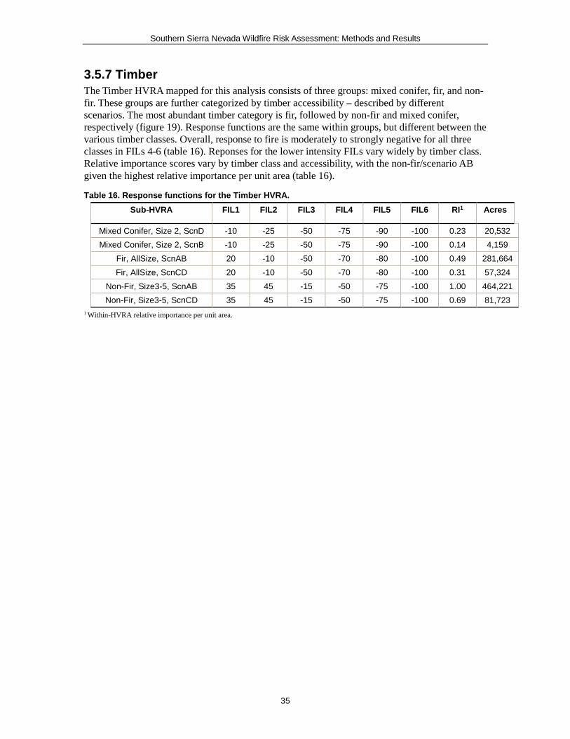
3.5.7 Timber The Timber HVRA mapped for this analysis consists of three groups: mixed conifer, fir, and non-fir. These groups are further categorized by timber accessibility – described by different scenarios. The most abundant timber category is fir, followed by non-fir and mixed conifer, respectively (figure 19). Response functions are the same within groups, but different between the various timber classes. Overall, response to fire is moderately to strongly negative for all three classes in FILs 4-6 (table 16). Reponses for the lower intensity FILs vary widely by timber class. Relative importance scores vary by timber class and accessibility, with the non-fir/scenario AB given the highest relative importance per unit area (table 16).

Table 16. Response functions for the Timber HVRA. Sub-HVRA FIL1 FIL2 FIL3 FIL4 FIL5 FIL6 RI1 Acres

Mixed Conifer, Size 2, ScnD -10 -25 -50 -75 -90 -100 0.23 20,532 Mixed Conifer, Size 2, ScnB -10 -25 -50 -75 -90 -100 0.14 4,159

Fir, AllSize, ScnAB 20 -10 -50 -70 -80 -100 0.49 281,664 Fir, AllSize, ScnCD 20 -10 -50 -70 -80 -100 0.31 57,324

Non-Fir, Size3-5, ScnAB 35 45 -15 -50 -75 -100 1.00 464,221 Non-Fir, Size3-5, ScnCD 35 45 -15 -50 -75 -100 0.69 81,723



36

Figure 19. Geospatial distribution of Timber in the southern Sierra wildfire risk assessment.


37

3.5.8 Watersheds Watersheds mapped in the project area consist of three vegetation types: herbaceous, shrub, and tree. Each type is categorized by erosion potential ranging from low to high potential. Treed watersheds are most common in the study area, followed by shrub and herbaceous, respectively (figure 20). Response to fire varies by vegetation type and erosion potential, however, in all three types, fire is neutral or beneficial in FIL1 and FIL2, while fires in FILs 3-6 are negative (table 17).

Relative importance was calculated in proportion to the surface drinking water importance scores attributed by the Forests to Faucets dataset (USDA Forest Service 2013).

Table 17. Response functions for the Watersheds HVRA. Sub-HVRA FIL1 FIL2 FIL3 FIL4 FIL5 FIL6 RI1 Acres

Herbaceous, high EP 0 0 -20 -40 -60 -80 - 70,409

Shrub, mod EP 20 0 -20 -40 -60 -80 - 478,124

Shrub, high EP 20 0 -30 -50 -80 -100 - 113,754

Tree, low EP 20 10 -20 -40 -60 -60 - 1,550,038

Tree, mod EP 20 10 -30 -50 -80 -80 - 1,313,823

Tree, high EP 20 0 -40 -60 -100 -100 - 482,147 1 Importance score in proportion to surface drinking water importance from Forests to Faucets.


38

Figure 20. Geospatial distribution of Watersheds in the southern Sierra wildfire risk assessment.


39

3.5.9 Vegetation Structure We assessed vegetation structure for the southern Sierra wildfire risk assessment using a custom approach, unique from all other HVRA. We mapped 15 biophysical setting (BpS) models (see Table 3) selected from the LANDFIRE BpS dataset (Rollins 2009) along with their respective S-Classes present on the landscape. The Vegetation Condition Assessment (VCA) methodology designed by Scott and others (2014) uses the six FIL classes produced by FSim to outline S-Class transition rules for fires burning at a given intensity. Table 18 highlights an example transition matrix for the California Montane Jeffrey & Ponderosa Pine Woodland BpS.

Each BpS/S-Class combination has a status within its respective landscape stratum, relative to historical reference conditions. After fire, and based on the transition experienced according to the FILs that occurred in that landscape, a given BpS/S-Class is likely to move from one status to another. In order to determine the net response from these transitions, we identified the value associated with a transition from one status to another (Table 19). Therefore, the total response for a given pixel depends both on the distribution of intensities across FILs 1-6 and the value placed on fire-caused transitions of S-Classes and their status on the landscape.

The within-HVRA relative importance weights assigned to each BpS are listed in Table 20. Five BpS classes received the full importance per unit area: Inter-Mountain Basins Subalpine Limber-Bristlecone Pine Woodland, California Montane Jeffrey & Ponderosa Pine Woodland, Great Basin Xeric Mixed Sagebrush Shrubland, California Lower Montane Blue Oak-Foothill Pine Woodland and Savanna, and Inter-Mountain Basins Montane Sagebrush Steppe. All other received less importance, at 0.75 per unit area.

For additional details regarding the VCA analysis and methodology, please refer to the VCA report (Helmbrecht 2015).

Table 18. Example S-Class transition matrix for the California Montane Jeffrey & Ponderosa Pine Woodland BpS model.

From FIL1 FIL2 FIL3 FIL4 FIL5 FIL6

A A A A A A A

B B B C C C A

C C C C C C A

D D D D D D A

E E E E D D A

Table 19. Response function values for fire-caused transitions from one status to another within an appropriately sized analysis unit for each BpS.

To Status

deficit similar surplus Ue

From Status

deficit 10 -50 -100 n/a

similar 75 10 -25 n/a

surplus 100 50 0 n/a

Ue n/a n/a n/a -10


40

Table 20. Listing of 15 BpS classes assessed and their relative importance per unit area. Biophysical Setting Relative importance

per unit area

Great Basin Pinyon-Juniper Woodland 0.75

Inter-Mountain Basins Subalpine Limber-Bristlecone Pine Woodland 1

Mediterranean California Dry-Mesic Mixed Conifer Forest and Woodland 0.75

Mediterranean California Mesic Mixed Conifer Forest and Woodland 0.75

California Montane Jeffrey & Ponderosa Pine Woodland 1

Mediterranean California Red Fir Forest - Cascades 0.75

Mediterranean California Red Fir Forest - Southern Sierra 0.75

Mediterranean California Subalpine Woodland 0.75

Sierra Nevada Subalpine Lodgepole Pine Forest and Woodland - Wet 0.75

Great Basin Xeric Mixed Sagebrush Shrubland 1

Inter-Mountain Basins Big Sagebrush Shrubland 0.75

Northern and Central California Dry-Mesic Chaparral 0.75

California Lower Montane Blue Oak-Foothill Pine Woodland and Savanna 1

Inter-Mountain Basins Montane Sagebrush Steppe 1

Central and Southern California Mixed Evergreen Woodland 0.75

3.6 Effects Analysis The cumulative result of the calculations presented in section 2.6 are the spatial grids of cNVC and eNVC presenting both the conditional and expected change in value from fire to all HVRA included in the analysis. Results are therefore limited to those pixel that have at least one HVRA and a non-zero burn probability. Both cNVC and eNVC reflect an HVRA’s response to fire and their relative importance within the context of the assessment, but eNVC captures both fire outcome and likelihood. Figure 21 shows cNVC results across the assessment area, with beneficial effects shown in blue and negative effects in cream, orange, and red. Much of the timber fuel in the middle of the assessment area and the shrub fuel along the northeastern portion experience positive fire outcomes – should a fire occur – while the majority of the western portion of the assessment area resulted in negative outcomes. Positive fire effects are largely attributable to beneficial responses for certain BpS models where fire had the desired effect of creating a distribution of SClass categories more representative of historical targets. Conversely, negative values seen along the western portion of the assessment area represent negative outcomes to watersheds, human habitation and infrastructure, slightly reduced by some positive outcomes due to vegetation. At first glance, it appears there are more beneficial effects on the landscape than there are negative. However, the overall mean cNVC value for the landscape is slightly negative at -0.57. Pixel values of negative outcomes range from less than zero to -1,368 while positive outcomes have a max value of 145. Though there are relatively few areas of orange and red pixels, their values could be up to nine times the value of a beneficial outcome, in the opposite direction.

Similar landscape trends exist in eNVC mapped in figure 21, with some subtle differences. Adjusting cNVC by fire likelihood (i.e. burn probability) narrows the range of values for both negative and positive outcomes. Many of the same areas, along with some new pixels, are still orange or red indicating potential for higher loss. However, the overall mean eNVC value of 0.12 reflects the degree to which loss is dampened by fire likelihood.


41

Finally, using FSim results from the lightning-only simulation, we mapped lightning-fire cNVC in figure 22. The results are nearly identical to large-fire cNVC, apart from a slight increase in pixels with beneficial outcomes in the northeastern portion of the assessment area due to the density of simulated lightning ignitions in that area (as indicated by the lighting simulation IDG shown in figure 4). Mean cNVC-lightning values reflect this change at 0.12 as compared to a negative mean for large-fire cNVC. Additionally, maximum cNVC values are nominally higher and loss is slightly greater than cNVC for large fires. These differences can be explained by the lack of suppression in the FSim simulation leading to larger fires with more pixels likely burning in the higher FIL categories.


42

Figure 21. Geospatial distribution of Expected Net Value Change (NVC) for all HVRA in the southern Sierra wildfire risk assessment.


43

Figure 22. Geospatial distribution of Conditional Net Value Change (NVC) for all HVRA based on lightning-only ignitions in the southern Sierra wildfire risk assessment.


44

3.7 Risk-Source Risk-source maps combine both pixel-based risk assessment results and fire perimeter polygons to identify each fire’s potential for positive or negative outcomes, and tie that information back to the fire’s ignition to identify spatial patterns on the landscape. Figure 23 is a plot of smoothed, NVCfire for large-fire ignitions and large-fire cNVC. This figure differs from figure 21 in that here we can generally identify where on the landscape fire ignitions tend to result in negative versus positive outcomes. Specifically, aggregated over 10,000 simulations, the average result of fires that start west of the Sierra crest is slightly negative to highly negative. The same is true of fires that start in the northern-most portion of the assessment area, extending down into west side of the range. Conversely, fires that start in the middle of the assessment area, where cNVC tends to be positive, result in positive outcomes, on average. This is also the case for fires igniting along the northeastern and eastern area-boundaries.

Overall risk-source patterns are similar for lightning-NVCfire (figure 24) as those described above for large-fire ignitions. The area of potential positive outcomes expanded considerably in the northeastern portion of the area, due to the tendency of lightning fires to start in areas of positive cNVC values (see the lighting simulation IDG shown in figure 4) and cNVC-lightning results in figure 22. Both positive and negative outcomes are highly magnified, likely due to fires growing unsuppressed and becoming very large, and therefore capable of a much stronger (negative or positive) average outcome in a given ignition-area. In terms of identifying where on the landscape lightning ignitions can grow unsuppressed with limited damage or positive outcomes, the middle and eastern/northeastern portions have the most potential. However, this map should only be used as a means to identify where on the landscape to begin a more refined analysis.

Whereas the eNVC and cNVC raster results inform decisions about fuel management, land-use planning, and asset hardening, the risk-source information discussed in this section is useful for planning the response to an unplanned ignition, whether of natural or human cause.


45

Figure 23. Large-fires as a source of NVC.


46

Figure 24. Lightning fires as a source of NVC.


47

4. References Calkin, D.E., Ager, A.A., Gilbertson-Day, J., Scott, J.H., Finney, M.A., Schrader-Patton, C.,

Quigley, T.M., Strittholt, J.R., Kaiden, J.D., 2010. Wildfire risk and hazard: procedures for the first approximation. Gen. Tech. Report RMRS-GTR-235. USDA Forest Service, Rocky Mountain Research Station, Fort Collins, CO.

Finney, M.A. 2005. The challenge of quantitative risk assessment for wildland fire. For. Ecol. Manage. 211, 97-108.

Helmbrecht, Don; Joe H. Scott; David Keefe. 2012. Little Belts Landscape Assessment: Vegetation Departure and Wildfire Threat Report. 46 p.

Rollins, M. G. 2009. LANDFIRE: a nationally consistent vegetation, wildland fire, and fuel assessment. International Journal of Wildland Fire. 18(3): 235-249.

Scott, Joe H.; R. E. Burgan. 2005. Standard fire behavior fuel models: A comprehensive set for use with Rothermel’s surface fire spread model. RMRS-GTR-153. Fort Collins, CO: U.S. Department of Agriculture, Forest Service, Rocky Mountain Research Station. 72 p.

Scott, Joe H. and Helmbrecht, Don. 2010. Wildfire threat to key resources on the Beaverhead-Deerlodge National Forest. Unpublished report to U.S. Department of Agriculture, Beaverhead-Deerlodge National Forest. [December 24, 2010]. 44 p.

Scott, J. H.; Helmbrecht, D. J.; Thompson, M. P. 2014. Assessing the expected effects of wildfire on vegetation condition on the Bridger-Teton National Forest, Wyoming, USA. Res. Note: RMRS-RN-71. Fort Collins, CO: U.S. Department of Agriculture, Forest Service, Rocky Mountain Research Station. 36 p.

Scott, Joe H. and Elizabeth D. Reinhardt. 2001. Assessing crown fire potential by linking models of surface and crown fire behavior. Res. Pap. RMRS-RP-29. Fort Collins, CO: U.S. Department of Agriculture, Forest Service, Rocky Mountain Research Station. 59 p.

USDA Forest Service. Forests to Faucets. Available online: http://www.fs.fed.us/ecosystemservices/FS_Efforts/forests2faucets.shtml (accessed on January 30, 2013)

USFS. 2014. RMRS Raster Utility. Available online at http://www.fs.fed.us/rm/raster-utility; last accessed April 15, 2015.

Helmbrecht, D.J. 2015. Vegetation Condition Assessment (VCA) Report for Southern Sierra Wildfire Risk Assessment.

Documents

Southern Sierra Nevada wildfire risk assessment: methods …a123.g.akamai.net/7/123/11558/abc123/forestservic... · 2016-05-26 · Southern Sierra Nevada Wildfire Risk Assessment: