Sascha HusaThe Sound of Space-timeSao Paulo, December 2018

Numerical Relativity

Sascha HusaThe Sound of Space-timeSao Paulo, December 2018

Numerical Relativity

Sascha HusaThe Sound of Space-timeSao Paulo, December 2018

Numerical Relativity

including alternative gravity

•Mathematical problems and exact solutions have dominated GR until recently.Deep insights gained: positive mass theorem, nonlinear stability of Minkowski spacetime . . .

•Astrophysics, cosmology, general understanding of the solution space of the EE require approximate solutions – analytical and numerical!

•Numerical solutions allow to study the equations (in principle) without simplifying physical assumptions, and allow mathematical control over the convergence of the approximation, and to estimate the errors!

Motivation: Numerical Relativity

What we will talk about, and what not.• Only talk about classical gravity, no computational quantum gravity!

• Solve Einstein Equations as PDEs, alternatively discretize geometry directly (e.g. Regge calculus, discrete differential forms, . . . ).

• 10 lectures + some practical problems:

1. Initial value problems for GR2. ODEs3. Hyperbolic Systems4. Numerics: Finite Differences5. Initial Data (for Black Holes)6. Gravitational wave signals7. Evolving Black holes, punctures and gauge conditions8. Computational Infrastructure9. Setting up a black hole simulation10.Working with results

Practical Problems• Choose 1 of 2 Tracks:

• ODEs: post-Newton black holes to leading order.

• Wave equation in 1+1 dimensions. Write code to solve a system of ODEs first (use method of lines for PDE).

• Choose a programming language you are familiar with. I can help best with Fortran, C, Python, Mathematica.

• Some worked out codes can be provided, but try yourself first.

Goals of these lectures

Be able to understand where NR results come from, how they are produced.

Understand the basic problems one faces in solving the Einstein equations, and the basic ideas of how some of these problems have been solved.

Create awareness for the long path from theory to quantitative results, as needed for observers (similar in particle physics!).

Be ready to get details from the literature.

Start to play with some code.

�5

But first, an announcement:

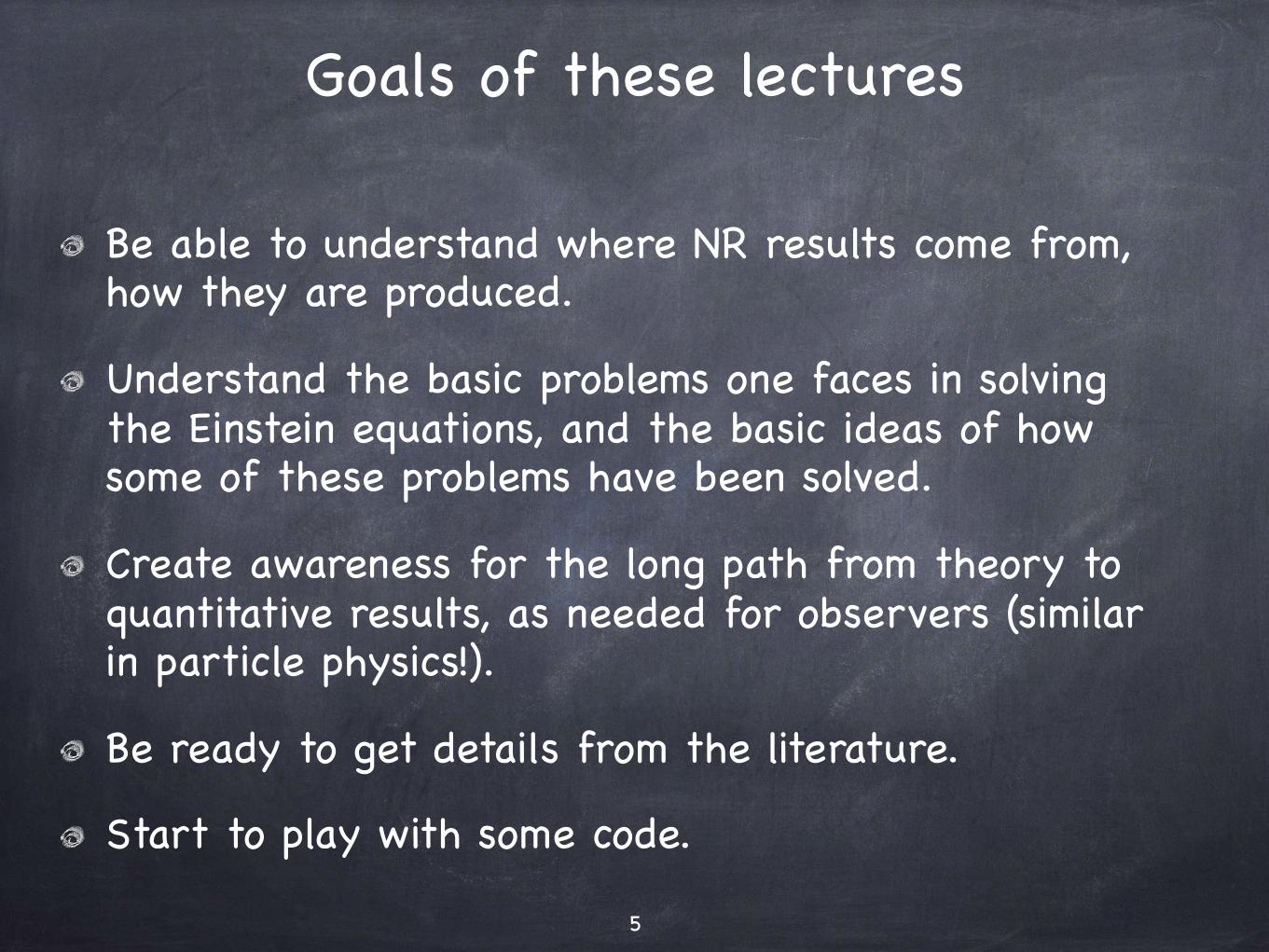
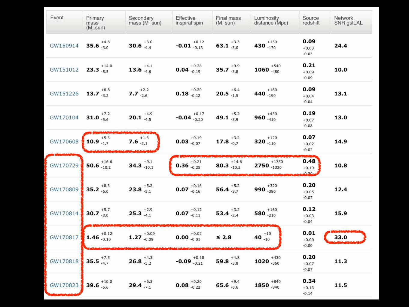
But first, an announcement:• Press release this morning, 11:00 local time:• LIGO + Virgo have released their compact binary coalescences catalogue

for the O1 + O2 observation runs.• Previously: 5 BBH GW events, 1 BBH LVT, 1 BNS

But first, an announcement:• Press release this morning, 11:00 local time:• LIGO + Virgo have released their compact binary coalescences catalogue

for the O1 + O2 observation runs.• Previously: 5 BBH GW events, 1 BBH LVT, 1 BNS

• Now we go to 11: 10 BBH mergers (LVT-> GW, 4 new), 1 BNS.• Open data + tutorials @ https://www.gw-openscience.org/catalog

But first, an announcement:• Press release this morning, 11:00 local time:• LIGO + Virgo have released their compact binary coalescences catalogue

for the O1 + O2 observation runs.• Previously: 5 BBH GW events, 1 BBH LVT, 1 BNS

• Now we go to 11: 10 BBH mergers (LVT-> GW, 4 new), 1 BNS.• Open data + tutorials @ https://www.gw-openscience.org/catalog

LIGO-Virgo | Frank Elavsky | Northwestern

1. Initial value problems for GR

• Classical physics is formulated in terms of PDEs for tensor fields.

• To understand a physical theory (GR, Maxwell, QCD, ...) requires to understand the space of solutions of the PDEs that describe it.

• What predictions to these solutions make for observations?

• Need a systematic = algorithmic way to find approximate solutions of PDEs: perturbation approaches, numerical analysis.

• EEs are intrinsically 4-dimensional How/where should we specify boundary conditions = select the physical solution?

• Time evolution problems: given initial data, does a unique time evolution exist? Does it depend continuously on the initial data? Predictability! Important source of physical intuition!

Q: Does the theory have an initial value formulation? Yes! Many!

Motivation: Initial Value Problem

Initial value problems

Choose coordinates for spacetime => ~ 10 coupled nonlinear wave eqs., complex source terms.

The known fundamental theories of nature(GR, elektro-weak theory, QCD (Yang-Mills)) are gauge theories, the presence of gauge freedom leads to constraints - restrictions on the space of possible initial data for a time evolution problems, which typically take the form of elliptic boundary value problems.Preserving constraints numerically well understood for E&M, not GR.

-— starting 1950’s -—>

• Can classify by the type of “problem” that can naturally be associated with a PDE: initial/initial boundary // boundary value problems.

• Standard types:

• hyperbolic, generalize wave equation: information propagates with finite speed

• parabolic: generalize heat equation, well posed only forward in time, information propagates instantaneously

• Schrödinger equation: information propagates instantaneously

• elliptic, e.g. Laplace equation:

Types of PDEs (linear for now)

�u(�x) = 0

u(�x, t),t = i�u(�x, t)

u(�x, t),t = �u(�x, t)

u(�x, t),tt = �u(�x, t)

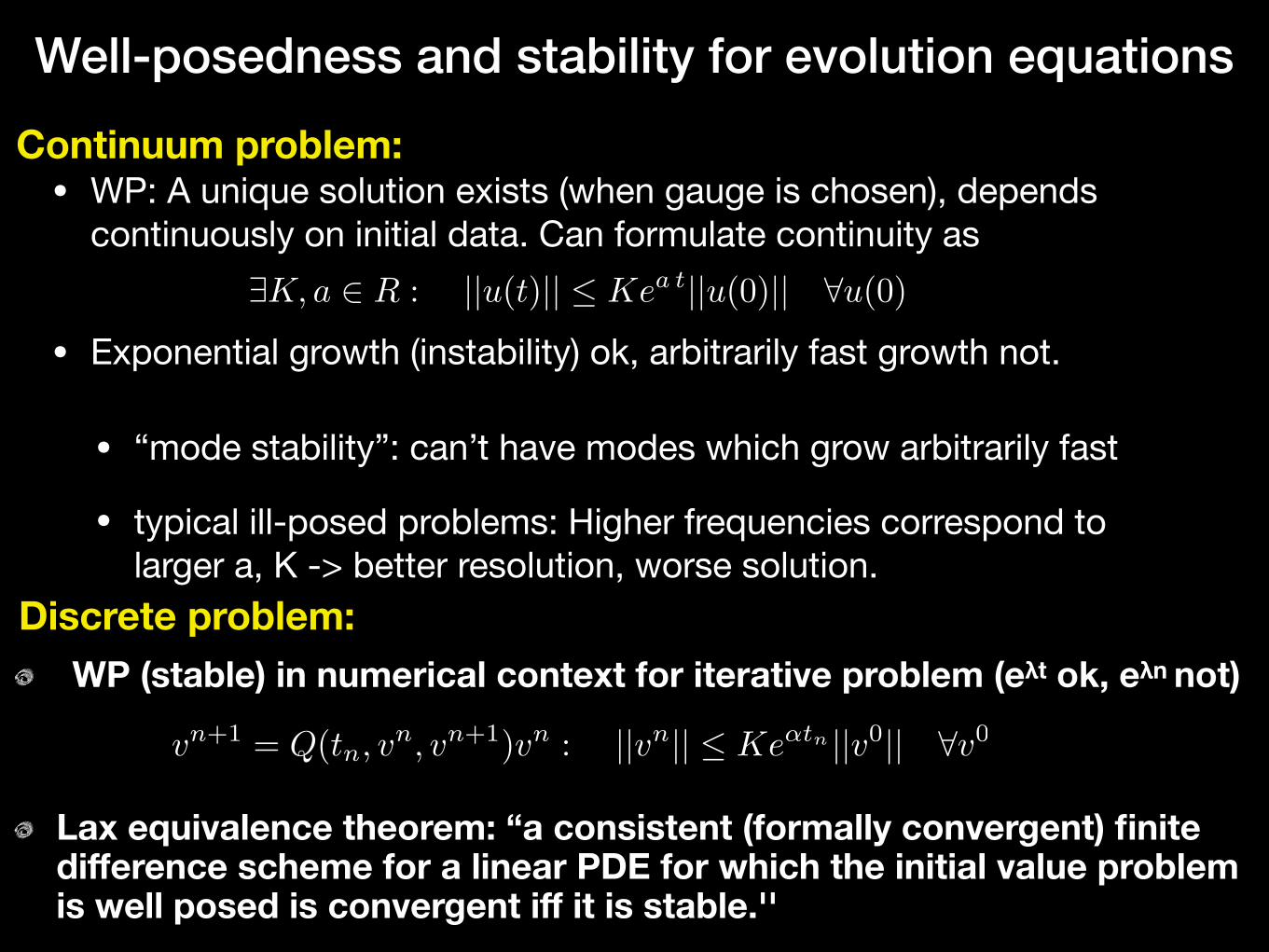
Well-posedness and stability for evolution equations

• WP: A unique solution exists (when gauge is chosen), depends continuously on initial data. Can formulate continuity as

• Exponential growth (instability) ok, arbitrarily fast growth not.

• “mode stability”: can’t have modes which grow arbitrarily fast

• typical ill-posed problems: Higher frequencies correspond to larger a, K -> better resolution, worse solution.

WP (stable) in numerical context for iterative problem (eλt ok, eλn not)

Lax equivalence theorem: “a consistent (formally convergent) finite difference scheme for a linear PDE for which the initial value problem is well posed is convergent iff it is stable.''

vn+1 = Q(tn, vn, vn+1)vn : ||vn|| � Ke�tn ||v0|| ⇥v0

⌅K, a ⇥ R : ||u(t)|| � Kea t||u(0)|| ⇤u(0)

Continuum problem:

Discrete problem:

Key to understand numerics: Conditioning• Consider model problem F(x,y) = 0

• How sensitive is the dependence y(x)?

• condition number K: worst possible effect on y when x is perturbed.

• consider perturbed eq. F(x + δx, y + δy) = 0,

• define

• K small: well conditioned, K large: ill conditioned,

• K=∞: ill-posed, unstable; K finite: well-posed

• NR: find well-posed PDE problem and for a given problem a gauge that makes K small!

K = sup�x

||�y||/||y||||�x||/||x||

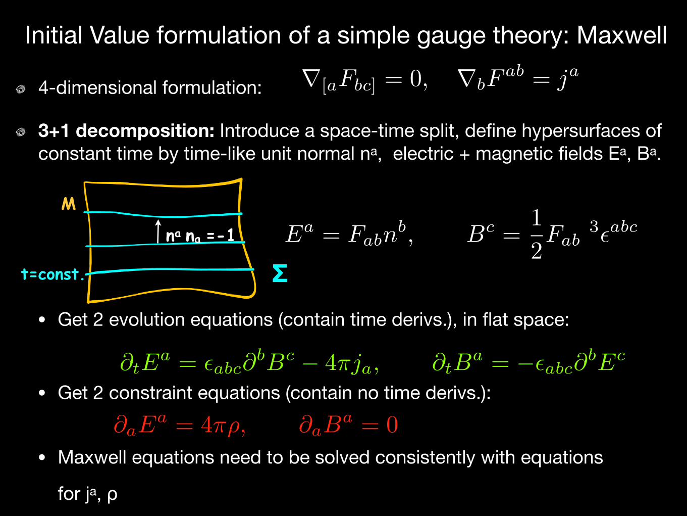
4-dimensional formulation:

3+1 decomposition: Introduce a space-time split, define hypersurfaces of constant time by time-like unit normal na, electric + magnetic fields Ea, Ba.

Initial Value formulation of a simple gauge theory: Maxwell

• Get 2 evolution equations (contain time derivs.), in flat space:

• Get 2 constraint equations (contain no time derivs.):

• Maxwell equations need to be solved consistently with equations

for ja, ρ

Ea = Fabnb, Bc =

1

2Fab

3�abc

⇤tEa = �abc⇤

bBc � 4⇥ja, ⇤tBa = ��abc⇤

bEc

⇤aEa = 4�⇥, ⇤aB

a = 0

na na =-1

M

t=const.

r[aFbc] = 0, rbFab = ja

Σ

Maxwell II

• Exercise: show that constraints propagate (always satisfied by virtue of the evolution equations, if satisfied at t=0)

• Initial value problem makes sense: constraints are preserved, for given initial data a unique time evolution exists, which depends continuously on initial data -> well-posed initial value problem

• Information propagates at the speed of light. We will soon understand connection between propagation speeds and the property of an IVP to be well-posed!

Maxwell III

• Using vector potential A additional gauge issues appear!Lorentz gauge -> Wave equation:

• Numerical ED is difficult (preserve constraints!), but well understood: analytical formulation, numerical algorithms, comparison with experiment!

• curved background:

• In collapsing case (K < 0) ) instability of constraints!

• Well-posedness is necessary but not sufficient to accurately approximate the continuum problem with finite precision!

• Solution for Maxwell: use . GR ?

LnDiEi = �KDiE

i, LnDiBi = �KDiB

i

pgEa,

pgBa

Fab = raAb �rbAa ) ra (raAb �rbAa) = jb

raAa = 0 ) raraAb = jb

Fast track 3+1 decomposition for GRSimplest way to get PDEs from the Einstein Equations:

Chose coordinates {xi , t} (i = 1, 2, 3),then “read off” metric in the form:

hab is a positive definite matrix (Riemannian metric on the 3-spaces of constant time), and 𝞪 ≧ 0.4 functions 𝞪, βi are freely specifiable, steer coordinate system through spacetime as time evolution proceeds – physical result is independent of this choice (diffeomorphism invariance).

PDEs resulting from ansatz are of 2nd order for h, split into 2 parts: 4 constraints (no second time derivatives) & 6 evolution equations.

Σ

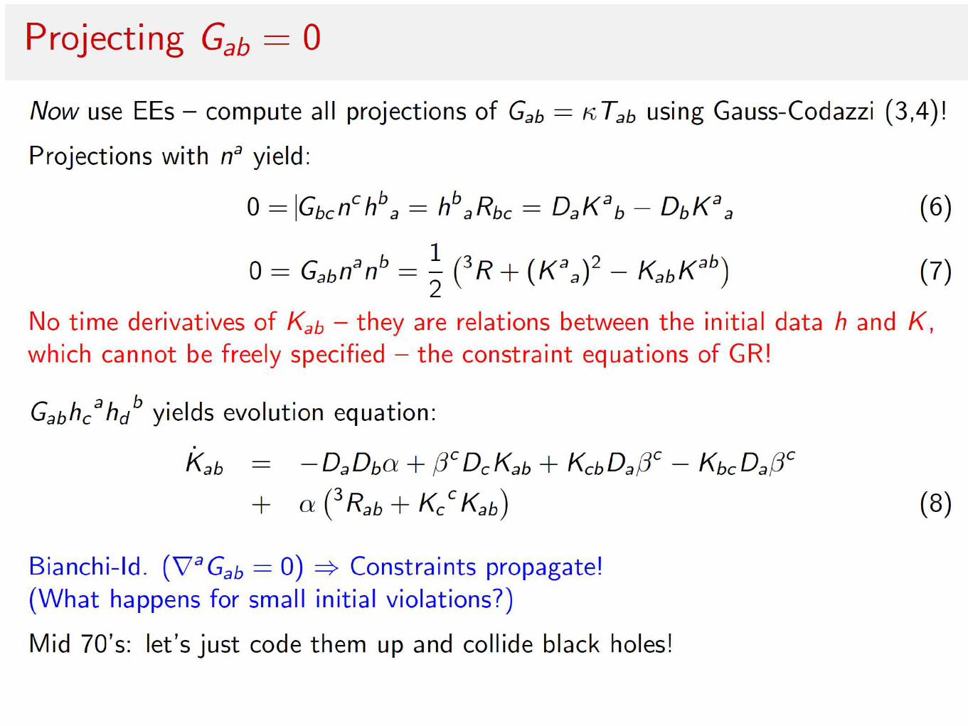
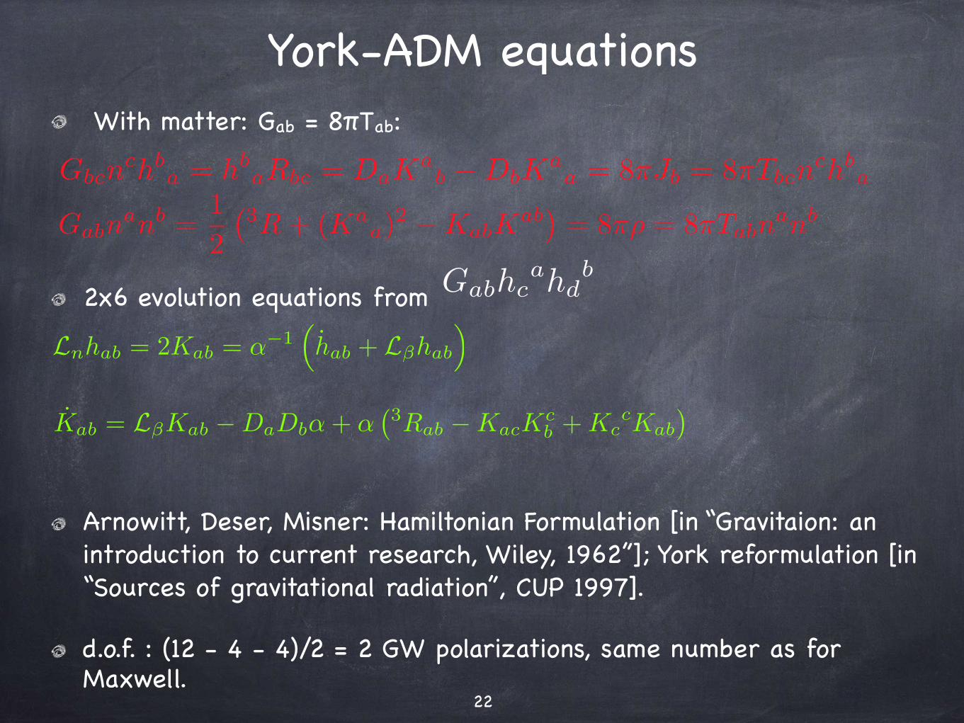
York-ADM equations With matter: Gab = 8πTab:

2x6 evolution equations from

Arnowitt, Deser, Misner: Hamiltonian Formulation [in “Gravitaion: an introduction to current research, Wiley, 1962”]; York reformulation [in “Sources of gravitational radiation”, CUP 1997].

d.o.f. : (12 - 4 - 4)/2 = 2 GW polarizations, same number as for Maxwell.

�22

Gabnanb =

1

2

�3R+ (Ka

a)2 �KabK

ab�= 8�⇥ = 8�Tabn

anb

Gbcnchb

a = hbaRbc = DaK

ab �DbK

aa = 8�Jb = 8�Tbcn

chba

Gabhcahd

b

Lnhab = 2Kab = ��1⇣hab + L�hab

⌘

Kab = L�Kab �DaDb�+ ��3Rab �KacK

cb +Kc

cKab

�

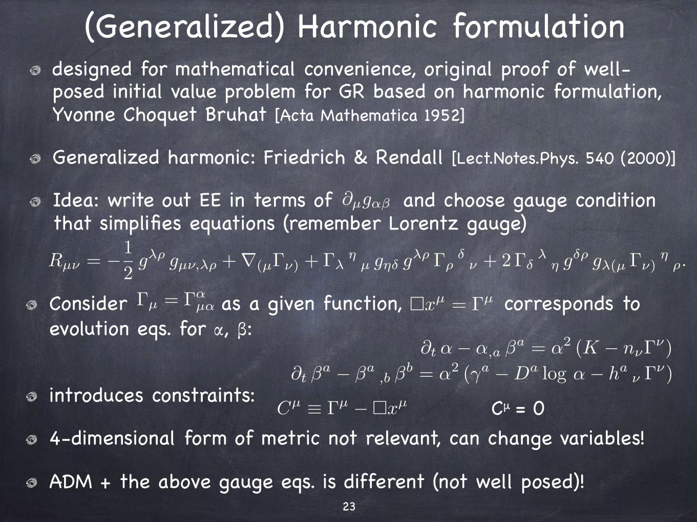
(Generalized) Harmonic formulationdesigned for mathematical convenience, original proof of well-posed initial value problem for GR based on harmonic formulation, Yvonne Choquet Bruhat [Acta Mathematica 1952]

Generalized harmonic: Friedrich & Rendall [Lect.Notes.Phys. 540 (2000)]

Idea: write out EE in terms of and choose gauge condition that simplifies equations (remember Lorentz gauge)

�23

Rµ⌅ = �1

2g⇤⇧ gµ⌅,⇤⇧ +r(µ�⌅) + �⇤

⇥µ g⇥� g

⇤⇧ �⇧�⌅ + 2��

⇤⇥ g

�⇧ g⇤(µ �⌅)⇥⇧.

⇤t �� �,a ⇥a = �2 (K � n��

�)

⌅t ⇥a � ⇥a

,b ⇥b = �2 (⇤a �Da log �� ha

� ��)

Cµ ⌘ �µ �⇤xµ

Consider as a given function, corresponds to evolution eqs. for α, β:

introduces constraints:

4-dimensional form of metric not relevant, can change variables!

ADM + the above gauge eqs. is different (not well posed)!

�µg�⇥

⇤xµ = �µ�µ = ��µ�

Cμ = 0

York-ADM emphasizes geometric intuition and gauge choice.

Harmonic emphasizes simplicity from a PDE point of view.

Until 1998 (BSSN!) mainstream NR was based on

Straightforward discretizations

formulations taylored to spherical symmetry: just worked

York-ADM equations: codes work in spherical symmetry, not in D>1

Progress in developing gauge conditions, horizon finders, ...! But unstable codes can’t tell what ideas work or do not.

In order to understand the strengths and weaknesses of each approach, and forge something that works, need to understand more about PDEs, numerical analysis, gauge conditions, BHs, ...

ADM vs Harmonic & some history

�24

f0 =

f(x+�x)� f(x��x)

2�x+O(�x

2)

• Let S be a 3-D “hypersurface of constant time” [an achronal (non-timelike) embedded submanifold of a manifold M (points of S can not communicate causally].

• Future domain of dependence D+(S) [analogous for D-(S)]:

• If nothing can travel faster than light, any signal sent to p ∈ D+(S) must have registered on S. Thus, given initial conditions on S, we should be able to predict what happens at p.

Domain of dependence

D+(S) =

⇢p 2 M

�� every past inextendible causal curve;through p intersects S.

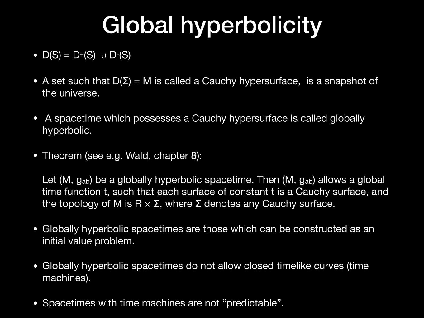
• D(S) = D+(S) ∪ D-(S)

• A set such that D(Σ) = M is called a Cauchy hypersurface, is a snapshot of the universe.

• A spacetime which possesses a Cauchy hypersurface is called globally hyperbolic.

• Theorem (see e.g. Wald, chapter 8): Let (M, gab) be a globally hyperbolic spacetime. Then (M, gab) allows a global time function t, such that each surface of constant t is a Cauchy surface, and the topology of M is R × Σ, where Σ denotes any Cauchy surface.

• Globally hyperbolic spacetimes are those which can be constructed as an initial value problem.

• Globally hyperbolic spacetimes do not allow closed timelike curves (time machines).

• Spacetimes with time machines are not “predictable”.

Global hyperbolicity

Beyond the Cauchy Problem

• Explain alternatives to Cauchy problem on blackboard:

• characteristic initial value problem

• Hyperboloidal initial value problem

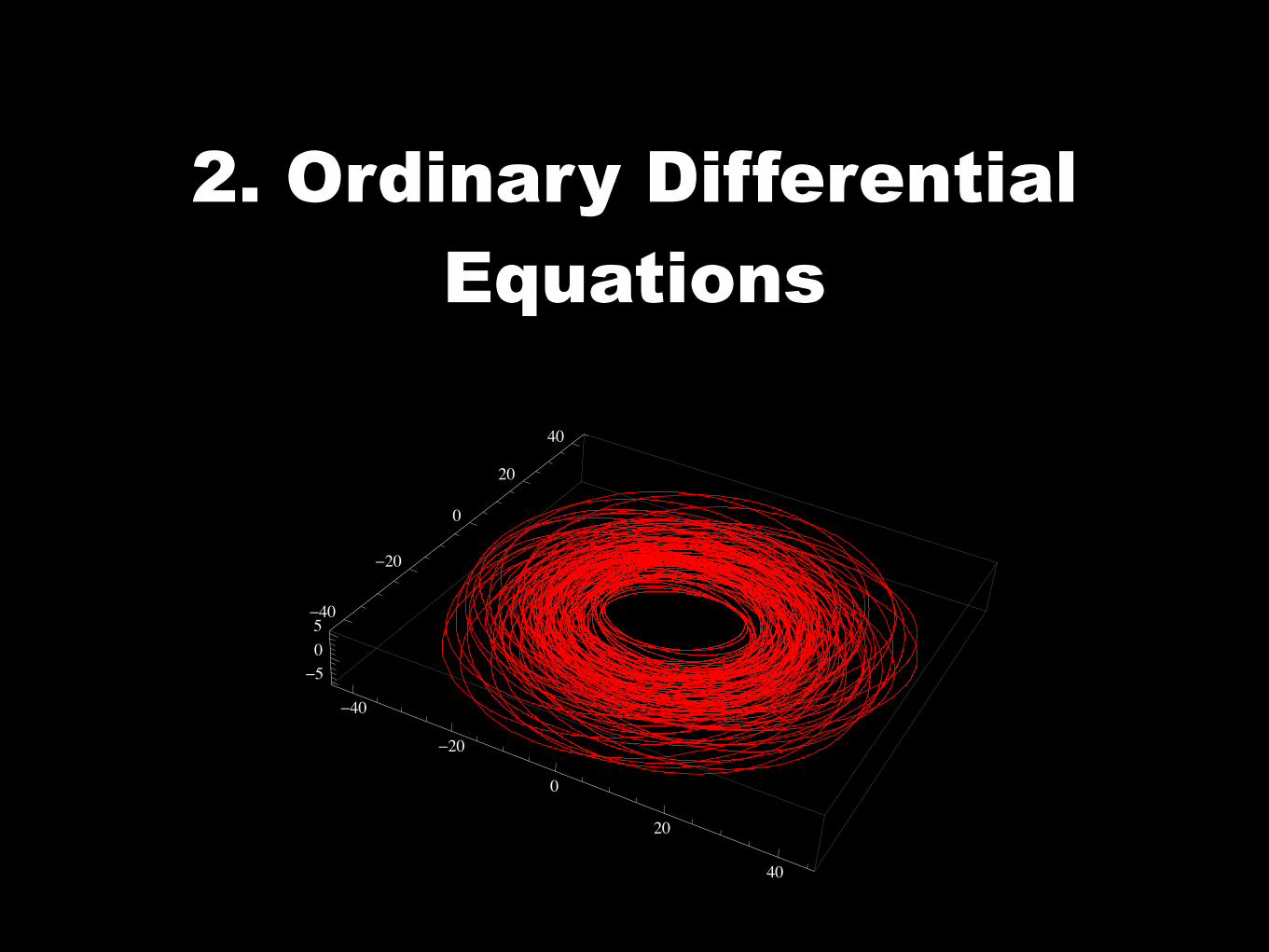
2. Ordinary Differential Equations

-40

-20

0

20

40

-40

-20

0

20

40

-505

ODEs in a nutshell• Don’t try to understand PDEs without understanding systems of ODEs.

• Can write ODE systems in first order differential form as a “normal form”: yi’(t) = Fi(t,yj)

• For higher differential order systems, introduce new variables, e.g. y’’(t) = F: v:=y’ -> {y’ = v, v’= F}

• Standard result of ODE theory:The ODE initial value problem is “well-posed”: Given initial datayi(t=t0), a unique solution yi(t) exists at least for some finite time t > t0.

• A global solution, i.e. for t->∞ may or may not exist.

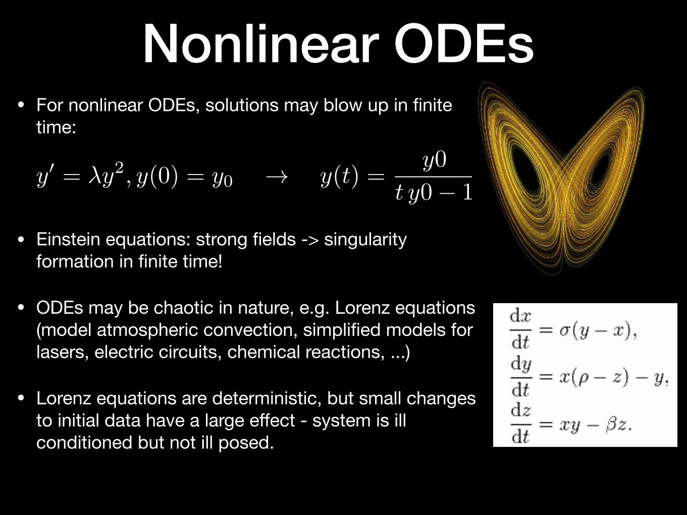
Nonlinear ODEs• For nonlinear ODEs, solutions may blow up in finite

time:

• Einstein equations: strong fields -> singularity formation in finite time!

• ODEs may be chaotic in nature, e.g. Lorenz equations (model atmospheric convection, simplified models for lasers, electric circuits, chemical reactions, ...)

• Lorenz equations are deterministic, but small changes to initial data have a large effect - system is ill conditioned but not ill posed.

y0 = �y2, y(0) = y0 ! y(t) =y0

t y0� 1

Linear systems of ODEs• Consider constant coefficient linear ODE systems: for nonlinear

equations, we can consider perturbations (can be stable or unstable), coefficients can be considered constant for a short time.

• constant coefficient linear ODE systems can be solved explicitly:

• Compute matrix exponential by transforming A to Jordan form:

• We can understand the behaviour of the solutions in terms of the eigenvalues and eigenvectors of the matrix A.

PAP�1 = D +N, Nn = 0 ) eiAkt = eiDkteiNkt = eiDktl=n�1X

l=0

N l kltl

l!

y0i = Aijyj ! yi(t) = eAi

jtyj(0)

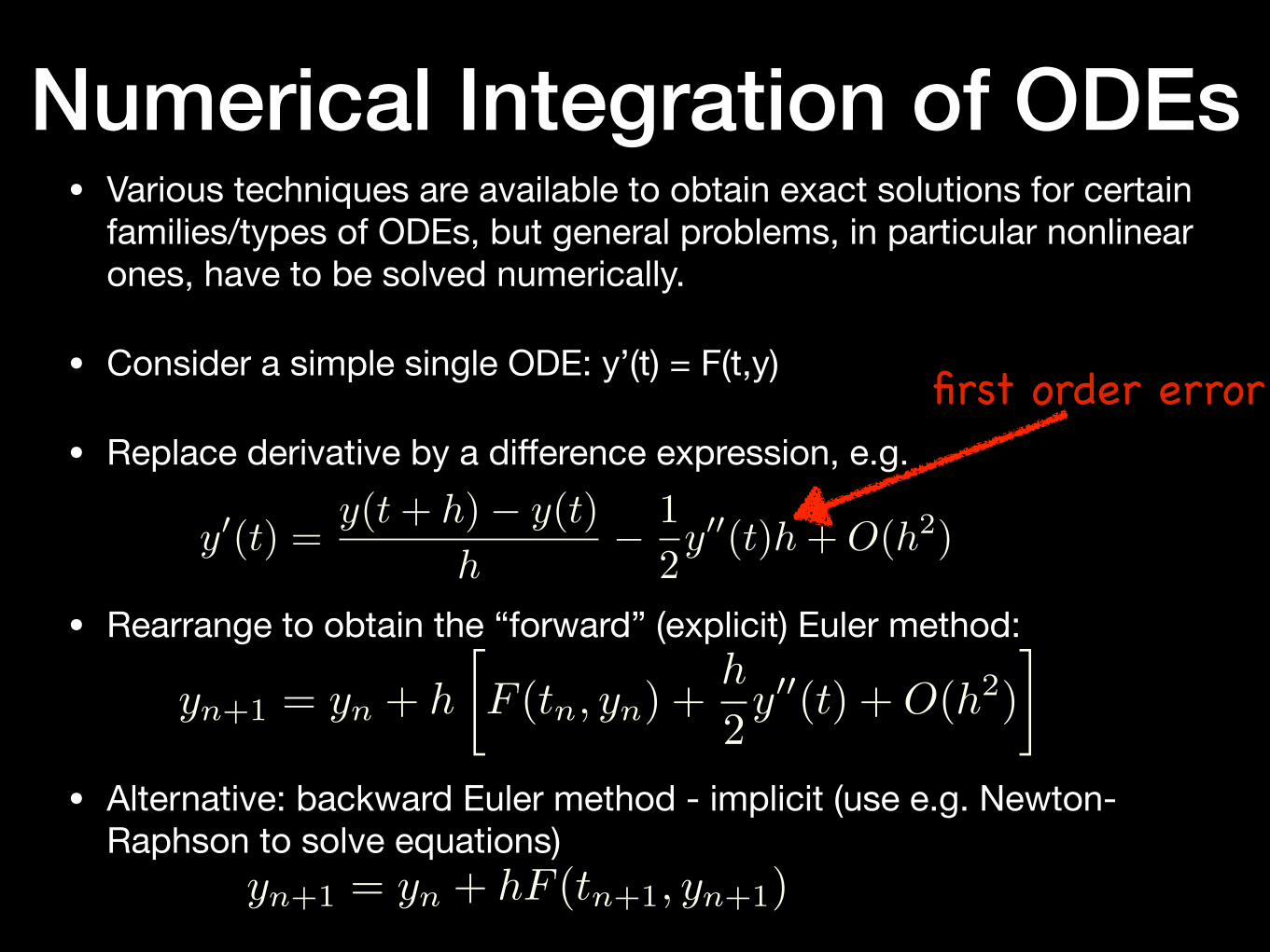
Numerical Integration of ODEs• Various techniques are available to obtain exact solutions for certain

families/types of ODEs, but general problems, in particular nonlinear ones, have to be solved numerically.

• Consider a simple single ODE: y’(t) = F(t,y)

• Replace derivative by a difference expression, e.g.

• Rearrange to obtain the “forward” (explicit) Euler method:

• Alternative: backward Euler method - implicit (use e.g. Newton-Raphson to solve equations)

y0(t) =

y(t+ h)� y(t)

h� 1

2y00(t)h+O(h2)

yn+1 = yn + hF (tn+1, yn+1)

first order error

yn+1 = yn + h

F (tn, yn) +

h

2y00(t) +O(h2)

�

Local truncation order• Error term in the Euler method is first order - we must be able to

do better! Use higher order approximations (Taylor)!

• But does Euler actually work? Does the numerical approximation converge? We are only interested in the continuum solution!

• Local truncation order: difference between exact and numerical solution in 1 step:

• The method is consistent if

• Method is convergent of order p if

• Euler methods are consistent and of order 1.

yn+1 = R(tn; yn+1, yn, {yn�k};h)

limh!0

�hn+1

h= 0

�hn+1 = O(hp+1)

�hn+1 = R(tn; yn+1, y(tn), y({tn�k});h)� y(tn+1)

Global truncation order

• Local error is relatively easy to control, but we need to know the global error - the error accumulated in all the steps one needs to reach a fixed time t.

• In the limit h-> 0 we need infinitely many steps, we can suspect that a “bad method” will not let us carry out this limit.

• In an unstable scheme, making a tiny error in each step will diverge in the limit.

Roundoff error• Truncation error of a finite difference scheme is not the only source of

error on a digital computer!

• We are using numbers with a finite precision, usually we are using double precision numbers as implemented in the machine hardware:

• Undefined values: INF or NAN (not a number) - exception handling tends to slow down computations.

• Don’t use single precision unless you really know what you are doing.

• Sometimes quadruple precision comes in handy, expect an order of magnitude slowdown.

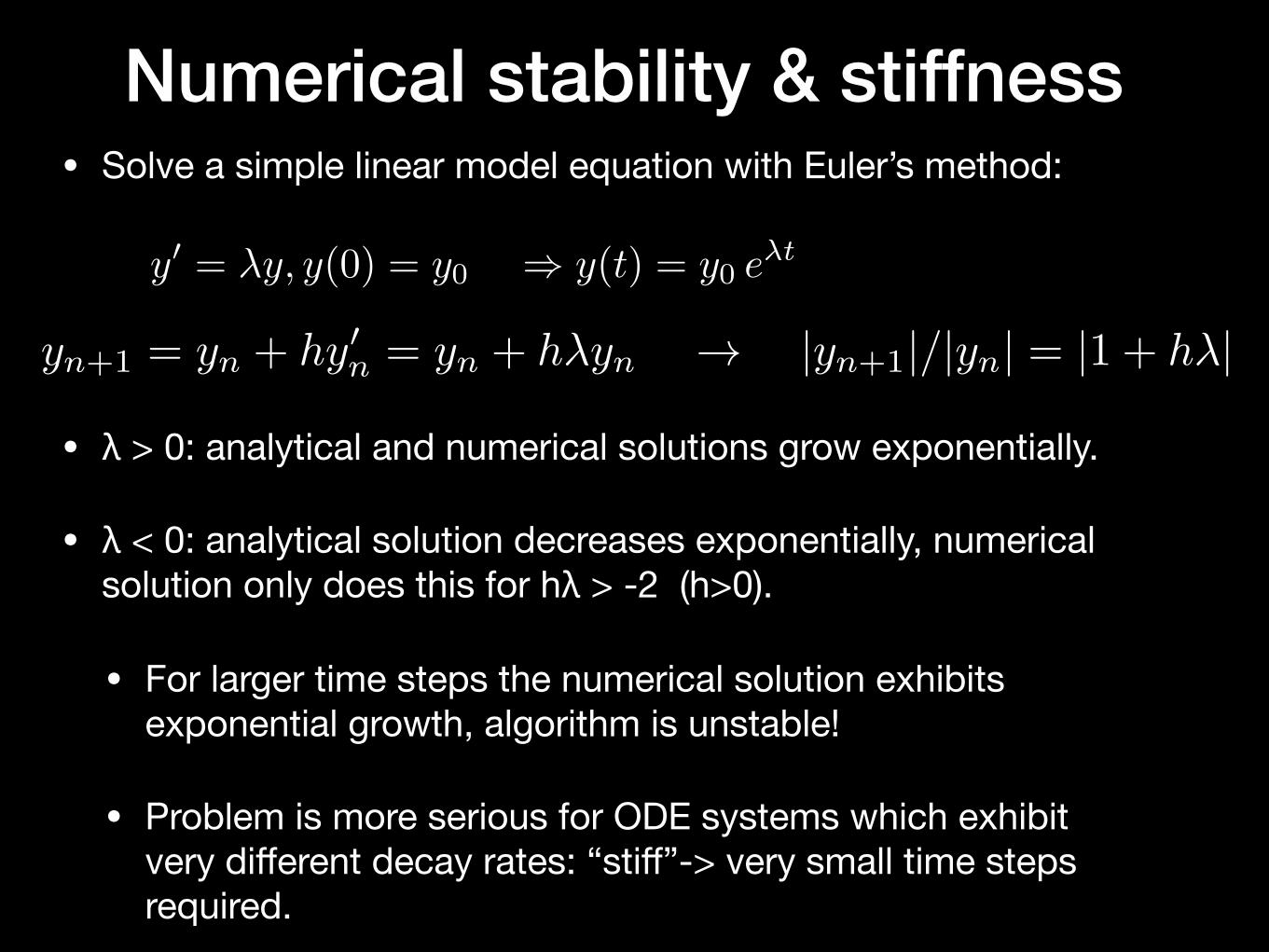
Numerical stability & stiffness• Solve a simple linear model equation with Euler’s method:

• λ > 0: analytical and numerical solutions grow exponentially.

• λ < 0: analytical solution decreases exponentially, numerical solution only does this for hλ > -2 (h>0).

• For larger time steps the numerical solution exhibits exponential growth, algorithm is unstable!

• Problem is more serious for ODE systems which exhibit very different decay rates: “stiff”-> very small time steps required.

yn+1 = yn + hy0n = yn + h�yn � |yn+1|/|yn| = |1 + h�|

y0 = �y, y(0) = y0 ) y(t) = y0 e�t

Higher order integration schemes• Basic idea is simple: approximate y’ more accurately, e.g. through a

higher order polynomial, compute coefficients with Taylor expansion.

• Standard class of methods: explicit Runge Kutta schemes, s stages:

• Method is consistent if:

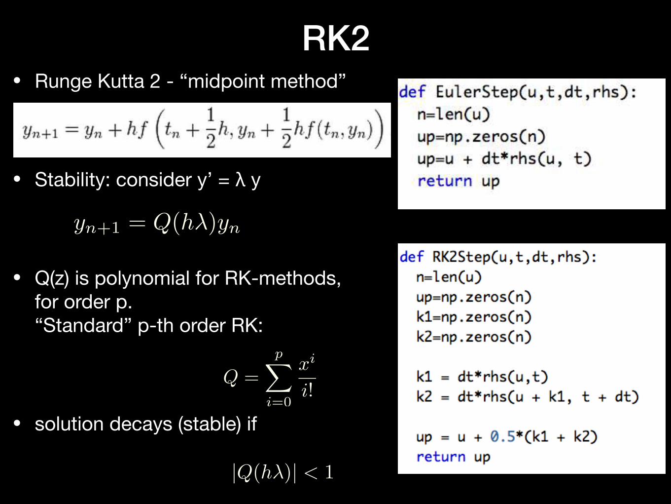
RK2• Runge Kutta 2 - “midpoint method”

• Stability: consider y’ = λ y

• Q(z) is polynomial for RK-methods, for order p.“Standard” p-th order RK:

• solution decays (stable) if

yn+1 = Q(h�)yn

|Q(h�)| < 1

Q =pX

i=0

xi

i!

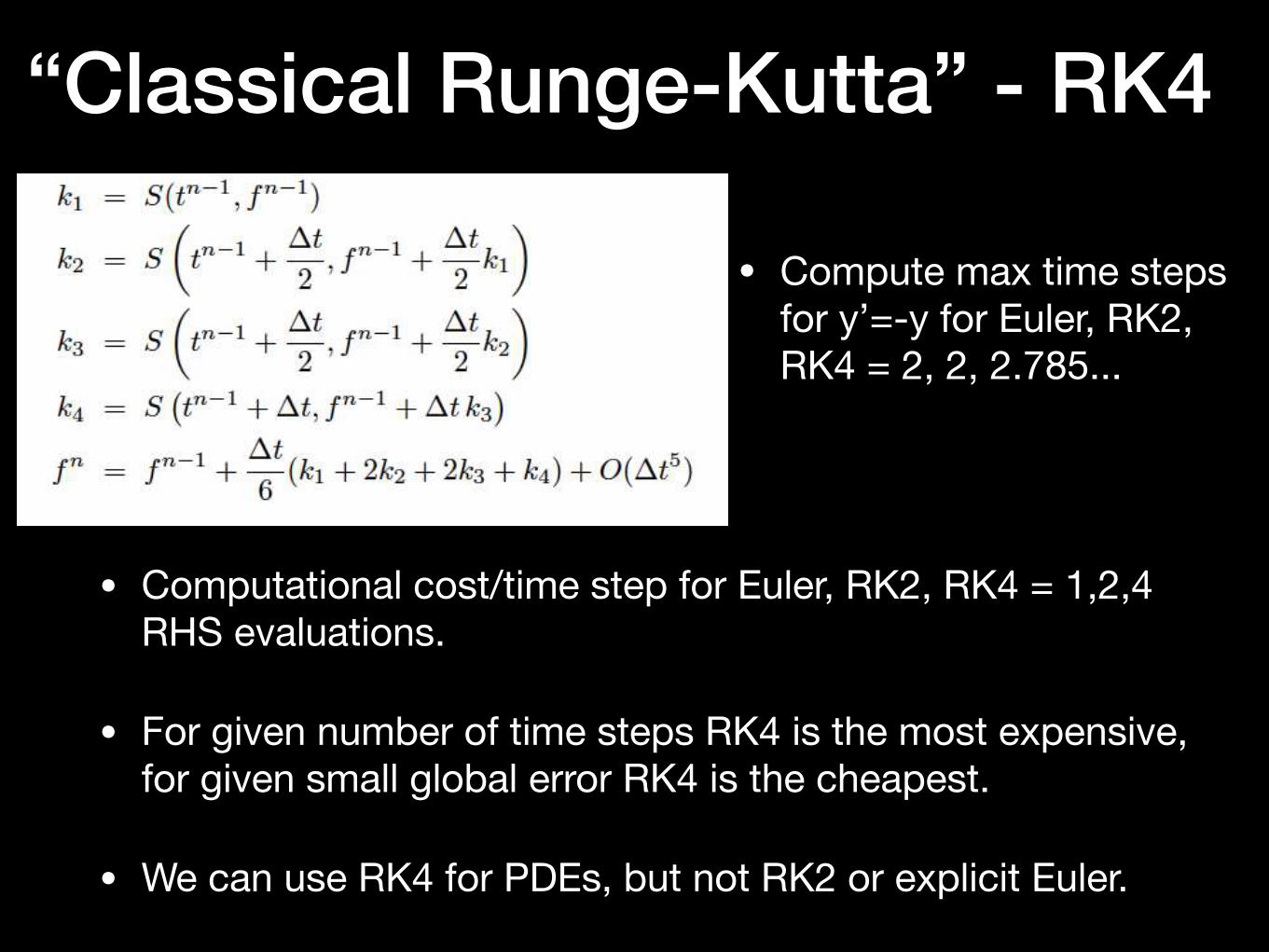
“Classical Runge-Kutta” - RK4

• Computational cost/time step for Euler, RK2, RK4 = 1,2,4 RHS evaluations.

• For given number of time steps RK4 is the most expensive, for given small global error RK4 is the cheapest.

• We can use RK4 for PDEs, but not RK2 or explicit Euler.

• Compute max time steps for y’=-y for Euler, RK2, RK4 = 2, 2, 2.785...

Other integration schemes• Higher order Runge Kutta methods can be constructed,

tuned toward efficieny, large time steps, ...

• Runge-Kutta methods are one-step methods. Multistep: reuse information from previous steps (e.g. Adams-Bashforth).

• Efficient solution of many problems requires a variable step size.

• Hamiltonian systems (classical mechanics): can exploit properties of such systems and construct integrators to e.g. preserve energy. Geometric integrators (e.g. symplectic integrators) correspond to canonical transformations.

Convergence

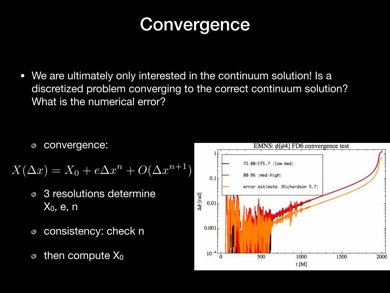
• We are ultimately only interested in the continuum solution! Is a discretized problem converging to the correct continuum solution? What is the numerical error?

X(�x) = X0 + e�xn +O(�x

n+1)

convergence:

3 resolutions determine X0, e, n

consistency: check n

then compute X0

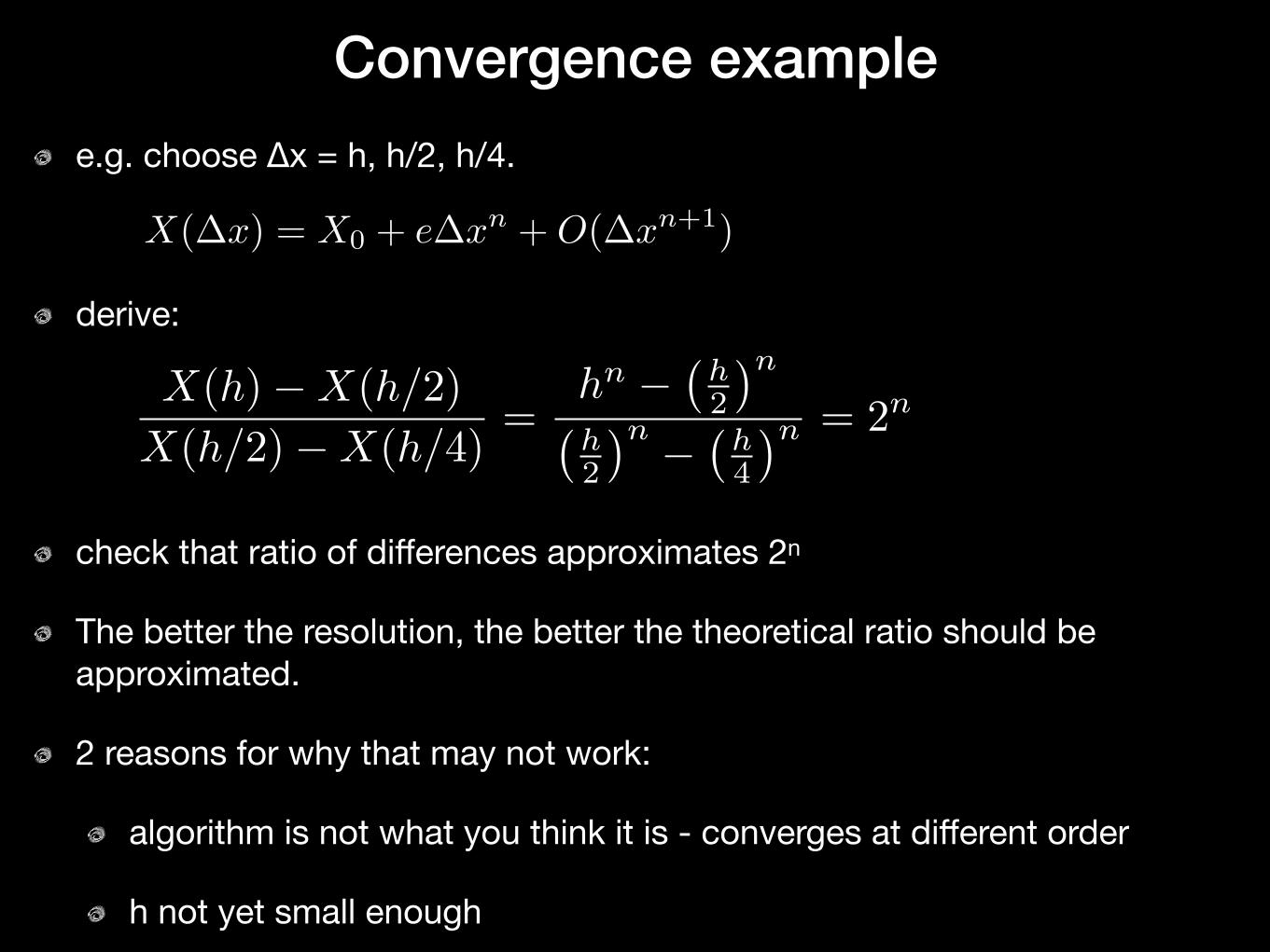
Convergence example

X(�x) = X0 + e�xn +O(�x

n+1)

e.g. choose Δx = h, h/2, h/4.

derive:

check that ratio of differences approximates 2n

The better the resolution, the better the theoretical ratio should be approximated.

2 reasons for why that may not work:

algorithm is not what you think it is - converges at different order

h not yet small enough

X(h)�X(h/2)

X(h/2)�X(h/4)=

hn ��h2

�n�h2

�n ��h4

�n = 2n