Spatial patterns and coexistence mechanisms in systems

with unidirectional flow

Frithjof Lutscher1

Department of Mathematical and Statistical Sciences, University of Alberta

Department of Biological Sciences, University of Calgary

flutscher@uottawa.ca

Edward McCauley

Department of Biological Sciences, University of Calgary

Calgary AB, T2N 1N4, CANADA

mccauley@ucalgary.ca

Mark A. Lewis

Department of Mathematical and Statistical Sciences and

Department of Biological Sciences, University of Alberta

Edmonton AB, T6G 2G1, CANADA

mlewis@math.ualberta.ca

1 Corresponding Author. Current Address: Department of Mathematics and Statis-

tics, University of Ottawa, Ottawa ON, K1N 6N5, Canada. Fax: ++1-613-562-5776

1

Abstract

River ecosystems are the prime example of environments where unidirectional flow influences

the dispersal of individuals. Spatial patterns of community composition and species replace-

ment emerge from complex interplays of hydrological, geochemical, biological, and ecological

factors. Local processes a!ecting algal dynamics are well understood, but a mechanistic basis

for large scale emerging patterns is lacking. To understand how these patterns could emerge

in rivers, we analyze a reaction-advection-di!usion model for two competitors in heteroge-

neous environments. The model supports waves that invade upstream up to a well-defined

”upstream invasion limit”. We discuss how these waves are produced and present their

key properties. We suggest that patterns of species replacement and coexistence along spa-

tial axes reflect stalled waves, produced from di!usion, advection, and species interactions.

Emergent spatial scales are plausible given parameter estimates for periphyton. Our results

apply to other systems with unidirectional flow such as prevailing winds or climate-change

scenarios.

Keywords: spatial competition; periphyton communities; invasion waves; coexistence; en-

vironmental heterogeneity; reaction-advection-di!usion equations

2

1 Introduction

One defining feature of river ecosystems is the presence of a strongly unidirectional flow. This

flow induces a heavy bias in the dispersal of individuals such as algae, invertebrates, and

stream insects. The question how a population can persist in rivers despite the flow-induced

washout has been termed the “drift paradox” (Muller, 1982), and has been addressed in recent

modeling papers (Lutscher et al., 2005; Pachepsky et al., 2005; Speirs and Gurney, 2001). In

this paper, we address the question where in a river a species can persist, given natural spatial

variation in resource levels. We also study how unidirectional flow influences the outcome of

competition, and in particular how it may mediate coexistence of two competitors.

We formulate our model for algal communities in rivers, however, our results apply to

many other scenarios of flow-through systems. Coastlines with long-shore currents present a

similar environment (Gaylord and Gaines, 2000), as do plug-flow reactors, which have been

used as models for the gut (Ballyk and Smith, 1999). Plants with windborn seeds in valleys

with prevailing wind directions face a similar “wash-out” problem. Finally, the pole-ward

movement of temperature isoclines due to global warming induces unidirectional “flow” by a

change of reference frame (Potapov and Lewis, 2004).

Algal communities in river ecosystems are highly dynamic. Species composition changes

significantly over time at a particular spatial location in response to temporal variation

in local nutrient concentrations and herbivore levels (Alvarez and Peckarsky, 2005; Hille-

brand, 2002; Henry and Fisher, 2003; Lamberti et al., 1989; Pringle, 1990), and physical

disturbances (McCormick and Stevenson, 1991; Peterson and Stevenson, 1992; Robinson and

Minshall, 1986). Larger scale spatial patterns in community composition and species replace-

ment emerge from these local interactions and some general features of these patterns have

been catalogued (Hill et al., 2000; Lavoie et al., 2003; Snyder et al., 2002; Wright and Li,

2002). While there has been extensive work done to understand processes at local spatial

3

scales (e.g. Hillebrand (2002) and citations above), there has been little work testing ideas as

to how larger-scale spatial patterns are produced. For example, larger-scale empirical pat-

terns based on the “River Continuum” (RCC) (Vannote et al., 1980) or “Serial Discontinuity

Concepts” (SDC) (Ward and Stanford, 1983) have been compiled. The RCC is often used

to predict the community composition of biotic groups as one moves down from headwater

streams to larger rivers. It assumes that benthic community composition reflects the relative

contribution of carbon loading from terrestrial versus in stream sources. The SDC modifies

the RCC by explicitly considering the direct (e.g. flow modification) and indirect (nutrient

cycling) hydrological e!ects of dams on modifying the relationship between external and in-

ternal loading, as well as the environmental influences on community composition. However,

the mechanistic basis for these patterns are poorly understood. Important linkages among

hydrology, biogeochemistry, ecological interactions, and population processes have been es-

tablished (Biggs et al., 1998; Dent et al., 2002; Fisher et al., 1998; Woodward and Hildrew,

2002), but general explanations for both the temporal and spatial dynamics of algal species

need to be elucidated and tested in river systems.

Recent experimental work investigating mechanisms producing basin-scale patterns in

algal community dynamics (Peterson, 1996; Cardinale et al., 2005) highlights the role of

dispersal mechanisms interacting with local processes, either following disturbance or along

nutrient gradients. To understand how these mechanisms give rise to spatial patterns and

temporal dynamics, we need a framework that incorporates ecological interactions and disper-

sal, along with advective flow down river. Table 1 summarizes the models used to understand

periphyton (benthic algae) dynamics in streams and rivers and their biological and physical

assumptions. These models typically include ecological interactions and the e!ect of advec-

tive flow but not dispersal. The situation is di!erent for terrestrial systems where extensive

work on spatial coexistence mechanisms has been undertaken (Amarasekare et al., 2004)

4

involving di!usion, but advective flow was not considered for obvious reasons.

In this paper, we use a strategic approach to understand how spatial competitive out-

comes among algal species are influenced by environmental heterogeneity in the presence of

advection and di!usion. Our goal is to understand how competing species invade and co-

exist in space under di!erent environmental scenarios. The mathematical formalism we use

abstracts much of the biology of the competitors into a phenomenological description of the

e!ects of changes in species density on growth rates of competitors.

In the next section, we present our model that consists of two reaction-advection-di!usion

equations coupled by Lotka-Volterra interaction terms. The analysis proceeds in three steps.

At first, we consider only a single species in a heterogeneous environment. We introduce the

notion of an upstream invasion limit. This point in space can be computed explicitly from

the model parameters. Numerical simulations reveal that an upstream-invading wave gets

stalled at this point. Secondly, we investigate numerically how two competitors can coexist

in a homogeneous environment. It turns out that boundary e!ects at the upstream boundary

may lead to coexistence. Finally, we extend the definition of upstream invasion limits to the

two-competitor case and show that coexistence can occur if the better competitor has its

invasion limit downstream from that of the weaker competitor. In the discussion, we use

published data to show that the spatial scales over which we expect coexistence to occur are

reasonably large.

2 Model Description

We start by focusing on the e!ect of competition on the abundance and distribution of

species in rivers. While competitive dynamics are well studied in ecology, the interaction

of competitive dynamics between species and the physical flow in a river, via di!usion and

advection in the river is complex. As we will show in this paper, this can produce a rich and

5

biologically interesting set of competitive outcomes that relate directly to river ecosystems.

While recognizing that competitive interactions in rivers are typically mediated via re-

source limitations (Son and Fujino, 2003), our approach is to take the simplest possible model

for competition that remains biologically interesting, that of Lotka-Volterra competition. To

this we add di!usive (random) and advective (directed) flow, as well spatial variation in

intrinsic growth rates (reflecting changing conditions for growth in the river system).

We consider two competing species in a river and denote N1,2(t, x) as their respective

densities at time t ! 0 and downstream location x. The equations read

!N1

!t= D1

!2N1

!x2" V1

!N1

!x+ N1(R1(x)"A11N1 "A12N2),

!N2

!t= D2

!2N2

!x2" V2

!N2

!x+ N2(R2(x)"A21N1 "A22N2),

(1)

where Ri(x) are the respective growth rates, Aij the inter- and intraspecific competition co-

e"cients, Di are the di!usion coe"cients and Vi the flow speeds. We assume that V1, V2 > 0

so that the flow is from left to right. Whereas flow speed might remain constant down-

stream or increase slightly in natural systems (Leopold, 1962), it is unclear whether the same

holds when large amounts of water are extracted from rivers for agricultural use or human

consumption. For simplicity, we consider a spatially constant speed here.

We would like to point out that the interaction terms in the model formulation are

somewhat di!erent from the standard notation. Usually, the growth rates Rj are factored

out of the brackets and the interaction coe"cients have dimension (density)!1, whereas in

our case the Aij have dimension (density * time)!1. Mathematically, the two formulations

are, of course, equivalent, but the one presented here and elsewhere (Potapov and Lewis,

2004; Shigesada et al., 1986) has certain advantages for our purposes. For example, the

formulation is consistent with Rj < 0. More importantly, for a logistic equation in a spatially

varying environment, one has the choice of varying the intrinsic growth rate, or the carrying

capacity or both. Since we aim for a simple model, we link the two and thereby reduce the

6

number of parameters, because the carrying capacities are now given by Kj = Rj/Ajj . For

convenience, we can rewrite the reaction term in (1) of species 1, say, as

R1N1

!1" N1 + "N2

K1

", (2)

where " = A12/A11, which relates our choice of parameters to the more commonly used

form of the equations. In particular, the parameters Aij , i #= j are simply multiples of the

commonly used competition coe"cients (Britton , 2003).

The case where growth rates R1,2 are constant was studied mathematically by Potapov

and Lewis (2004), in particular when the river is very long (mathematically speaking, an

unbounded domain). There, the coupled growth and dispersal can lead to population spread

in space. The invasion speed at which the population spreads is a key quantity that will play

a role later in this paper. It is easiest to first consider the case for (1) with a single species

and no advective flow (N2 = 0 and V1 = 0). This is simply logistic growth with random

dispersal, or the so-called Fisher equation, which has invasion speed 2$

D1R1 (Fisher, 1937).

If V1 #= 0 the invasion speed in the direction of the flow is given by 2$

D1R1 + V1, whereas

the speed in the opposite direction is given by 2$

D1R1"V1. In particular, the invasion does

not move against the flow when V1 > 2$

D1R1 (Pachepsky et al., 2005).

In two-species competition models, one can study the case where a superior competitor

(say species 1) outcompetes the other competitor, and spreads spatially into the (infinite)

region previously occupied by species 2. For Lotka-Volterra competition as above, with

V1,2 = 0, the speed at which the weaker competitor retreats is identical to the speed at which

the stronger one advances. This replacement process occurs at speed

2#

D1(R1 "R2A12/A22) (3)

provided the following two conditions are satisfied (Lewis et al., 2002)

D2

D1% 2,

A12A21A11A22

" 1

1" A12R2A22R1

% R1

R2

!2" D2

D1

". (4)

7

These conditions are su"cient but not necessary as numerical simulations show. However,

the spreading speed can be much larger if the conditions are violated (Lewis et al., 2002). In

all simulations presented below, conditions (4) are satisfied, and hence the spreading speed

of the better competitor into the domain occupied by the weaker competitor is given by (3).

A more accurate depiction of a river is a body of water of finite length L. We can

consider equations (1) on a bounded domain [0, L] where, of course, population spread cannot

continually happen at constant speed. We consider x = 0 to be the top of the river where

individuals neither leave nor enter (zero flux). In contrast to previous modeling approaches

(Speirs and Gurney, 2001; Pachepsky et al., 2005) we consider a river where the downstream

boundary at x = L is “far away,” i.e., has no influence on upstream processes. These two

assumptions are encapsulated in the so-called Danckwerts boundary conditions (Ballyk et al.,

1998)

Di!Ni

!x" ViNi = 0, x = 0,

!Ni

!x= 0, x = L, i = 1, 2. (5)

The first of these boundary conditions describes zero flux at the top of the river, and the

second describes zero variation in population density with space at the downstream boundary.

For a derivation and discussion of these boundary conditions from a random-walk perspective,

see Lutscher et al. (in press). From here on, we make the following simplifying assumptions:

1. Di!usion and flow speeds are the same for both species, D1 = D2 = D,V1 = V2 = V.

2. Growth rates are linear and non-decreasing, and R2/R1 = # =const., i.e.,

R1(x) = RU + (RL "RU )x, RU % RL, R2(x) = #R1(x), (6)

where the indices U,L stand for the upper and lower end of the river section.

The main focus in sections 3 and 4 below is on numerical results, their biological interpre-

tation and significance. Here we briefly give some background on analytical results and the

numerical methods used. In the case of a single equation (e.g., N2 = 0) and positive initial

8

data, all solutions converge to a unique stable equilibrium. Depending on parameter values,

this equilibrium is either zero (if zero is locally stable) or positive (if zero is unstable). This

result follows from the shape of the reaction term (logistic growth) and the fact that the

equation satisfies a maximum principle. As a consequence, the outcome of numerical sim-

ulations is independent of the chosen initial conditions. The 2-species system is a so-called

“monotone system” (Smith, 1995). When parameters are chosen such that either species

can invade the other at equilibrium, the theory of monotone systems predicts that there

is a coexistence equilibrium, but it may not be unique (Smith, 1995). Therefore, the final

outcome of simulations might depend on initial values, however, we studied the full system

(1) numerically for a wide range of initial data, and found again that the final outcome is

independent of initial values. (The outcome does, of course, depend on parameter values.)

For monotone initial values, solutions formed invading or retreating waves. Since neither the

qualitative behavior nor the final outcome of the simulations depends on the initial location

of the species, we chose to illustrate the results using initial conditions that allowed most

clearly to observe the di!erent processes and time scales involved. For numerical simula-

tions, we chose an unconditionally stable implicit finite-di!erence scheme. Derivatives were

approximated by finite di!erences, backward in time, central in space for the di!usion term,

and upwind for the advection term (Strickwerda, 1989).

For numerical simulations we introduced the nondimensional quantities

t" = t maxx

R1(x) = tRL, x" =x

L, di =

Di

L2RL, vi =

Vi

LRL, ni =

AiiNi

RL. (7)

Then the nondimensionalized system is then given by

!n1

!t= d1

!2n1

!x2" v1

!n1

!x+ n1(r1 " n1 " a12n2),

!n2

!t= d2

!2n2

!x2" v2

!n2

!x+ n2(r2 " a21n1 " n2),

(8)

where now

ri(x) =Ri(x)RL

, aij =Aij

Ajj. (9)

9

We used some analytical and some numerical methods to compare the e!ects of the down-

stream boundary conditions (5) chosen here to the “hostile” boundary conditions Ni(t, L) = 0

used elsewhere (Speirs and Gurney, 2001; Pachepsky et al., 2005). The qualitative di!erences

occur only at the downstream end for long enough domains, where the solutions are forced

to zero with hostile conditions. If the domain is long enough to support the populations,

then the upstream end is not a!ected by the downstream boundary conditions. The critical

domain size for hostile conditions is larger than for the Danckwerts conditions.

3 Results

Single species

If only one species is present, and growth is constant in space, i.e., R(x) = R, equations (1)

reduce to a single equation that was analyzed by Speirs and Gurney (2001) and Pachepsky

et al. (2005), see also Murray (1983) for a more general mathematical treatment in higher

space dimension. Their main results in the present context are that, if the stream is arbitrarily

long, the species can invade in the upstream direction if and only if the invasion condition

V < 2$

DR is satisfied. Upstream invasion occurs in the form of a traveling wave, moving

against the flow at constant speed. When the river becomes shorter, the total amount of

habitat available to the species is reduced. Speirs and Gurney (2001) showed that there is

a critical domain size, a length of river that is so short that the species cannot survive any

further reduction of habitat.

We investigate the case when the growth rate varies spatially. We shall not be concerned

whether the species can persist at all but rather where it will be present. We consider a

river long enough to exceed the critical domain size where the growth rate varies spatially in

such a way that the invasion condition holds at the bottom of the stream but is violated at

10

the top. Then the monotonic increase in growth rate with increasing distance downstream

implies that there is a unique point x# in the domain where

V = 2#

DR(x#). (10)

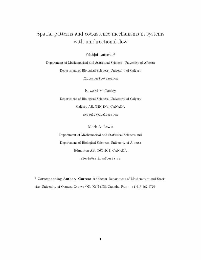
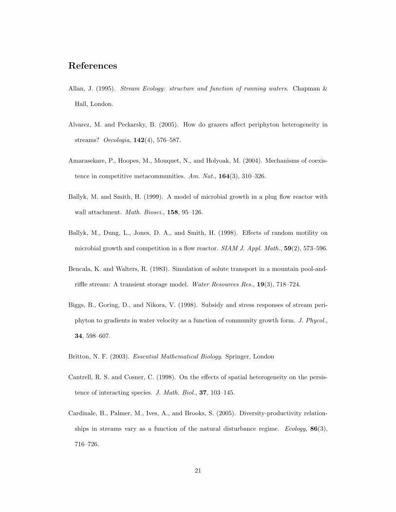
The resulting behavior is summarized in the following points and illustrated in Figure 1.

1. The species persists with near-zero density at the top and almost carrying capacity at

the bottom.

2. The location of the transition is predicted by the invasion limit x#.

3. If the species is initially located at the downstream end, then it spreads upstream in a

wavefront that stalls at the invasion limit.

The steepness of the transition between the two states depends on the parameters. The

steepness increases as D decreases provided the product DR(x#) is held constant so that

the invasion limit is fixed. We explored several shapes of non-linear spatially varying growth

rates R(x), all monotone increasing so that the upstream invasion limit x# is well-defined.

In all cases, we observed the same qualitative behavior as in the case for linearly increasing

growth rates described above.

Competing species

The non-spatial competition model allows for three di!erent outcomes (coexistence, competi-

tive exclusion, founder control), depending on parameters. We concentrate on the case where

species 1 outcompetes species 2 in the non-spatial model, but species 2 has the higher growth

rate at low densities, i.e., R2/R1 = # > 1, A12# < A22, A21 > #A11. These conditions depend

only on the ratio # of the growth rates and are therefore independent of spatial location.

In the homogeneous spatial model with constant growth rates, the outcome of spatial

movement and competition depends on the magnitude of the flow speed. For small flow speed,

11

species 1 invades all the way to the upstream boundary, x = 0, at a density close to carrying

capacity. Species 2 goes extinct as predicted by the non-spatial model. At intermediate

speeds, coexistence is possible in a boundary layer near the upstream boundary, because the

density of species 1 and hence its e!ect on species 2 is small near the upstream boundary.

The coexistence region grows with increasing flow speed. For higher speeds, the competitive

outcome is reversed as species 2 persists in the whole domain whereas species 1 gets washed

downstream, even though the flow speed would allow persistence in the absence of species 2.

If the speed is so large that the invasion condition for species 2 is violated, then both species

go extinct.

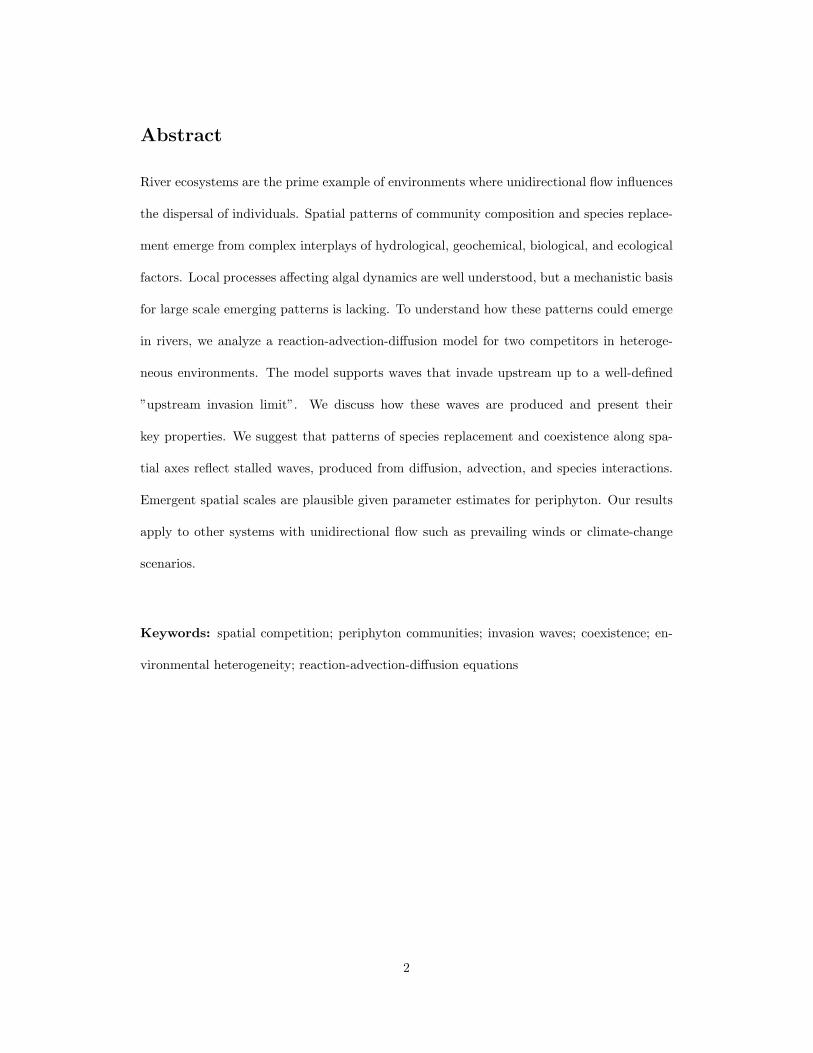
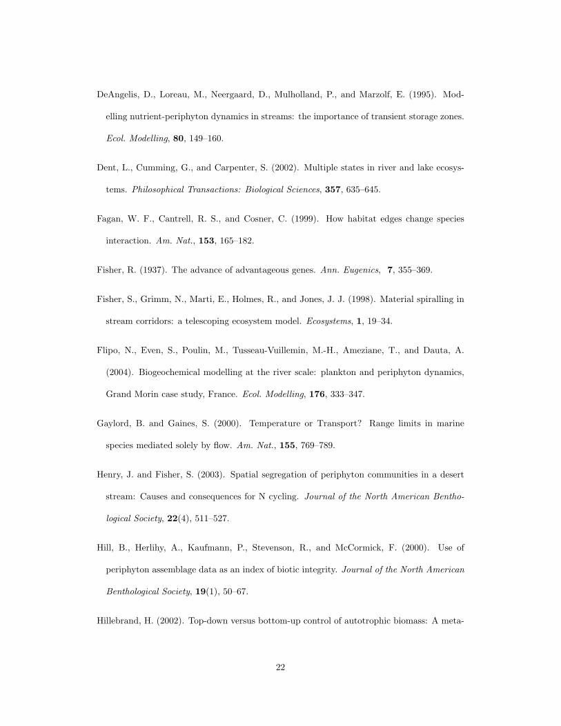
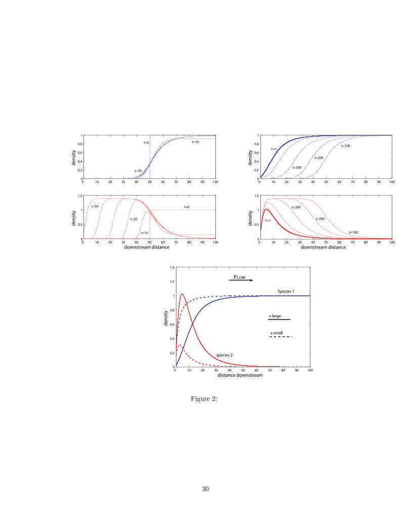
Figure 2 depicts how in the case of intermediate flow speeds both species invade upstream.

Species 2 spreads faster initially but is being outcompeted downstream by species 1. The

upstream spread of species 1 is slower, but the population reaches the upper end of the stream

eventually and allows only a small region of coexistence with the inferior competitor near

the boundary. Potapov and Lewis (2004) investigated the steady states of a similar system

in much more detail.

When growth rates vary spatially, each species has its invasion limit in the absence of the

competitor, denoted by x#1,2 and given implicitly by (10). Due to the higher growth rate for

species 2, the invasion limit of species 2 is upstream of that of species 1, i.e., x#2 < x#1. There is

a second invasion limit for each species, obtained by fixing the density of the competitor at its

single-species carrying capacity to find a reduced growth rate Ri"AijNj , with Nj = Rj/Ajj .

This second invasion limit is denoted by x##i and defined implicitly by

V = 2$

D[Ri(x##i )"AijNj(x##i )], (11)

This definition reduces to (10) in the absence of the other species (AijNj = 0). Because

competition has the e!ect of reducing net growth rates, the single-species invasion limit is

upstream of the invasion limit with the competitor at carrying capacity, i.e. x#i < x##i .

12

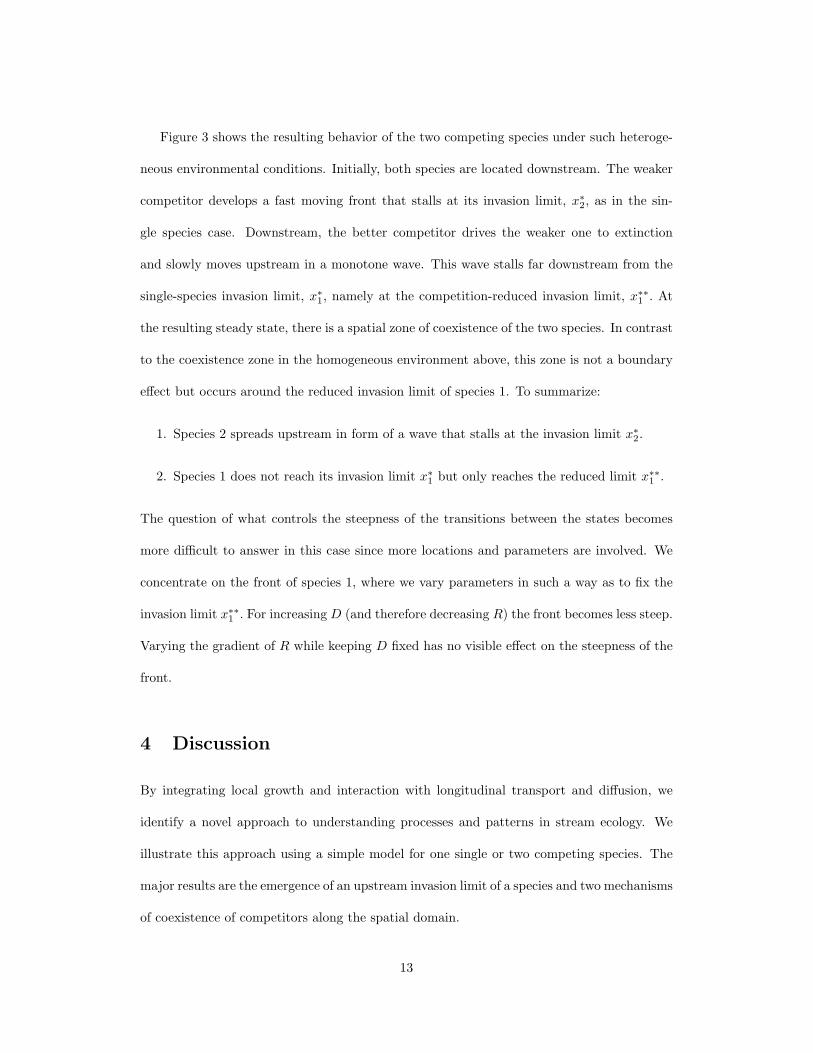
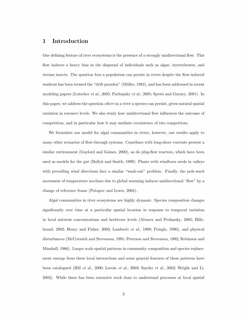
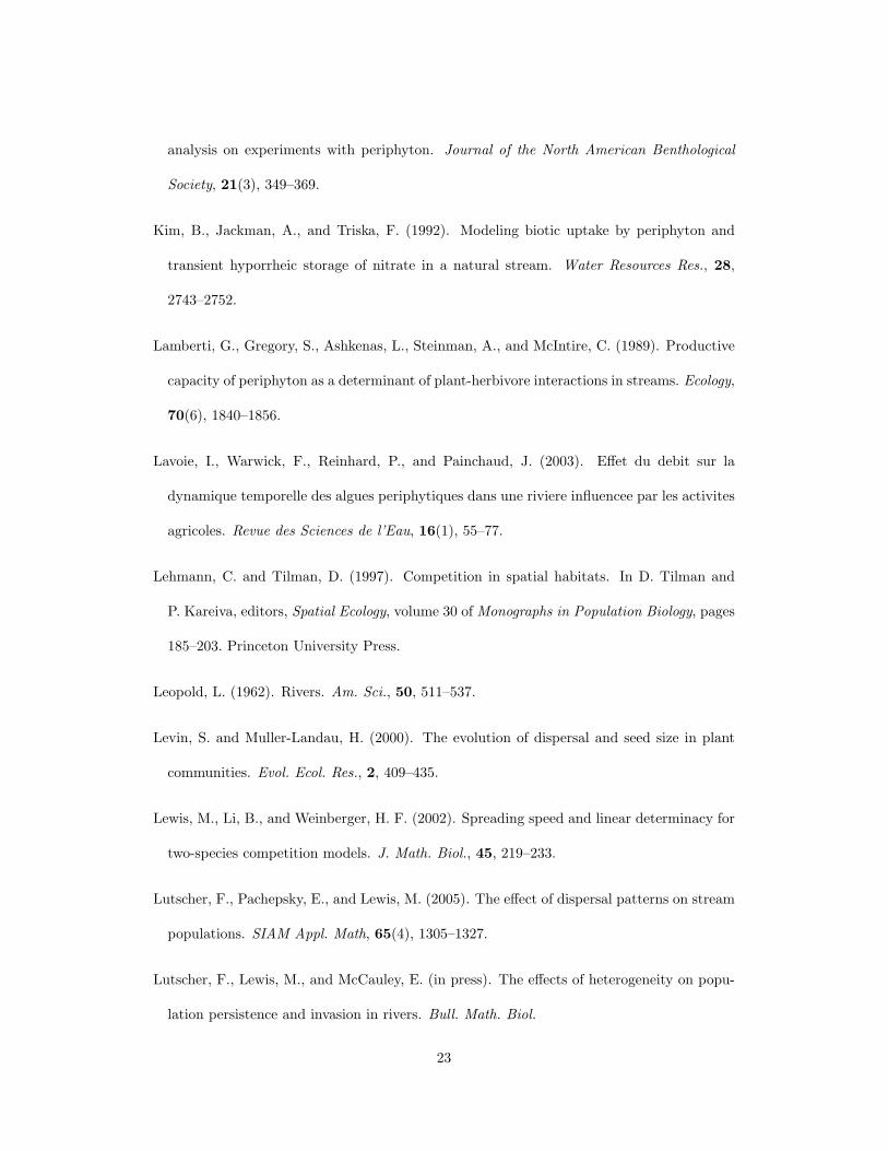
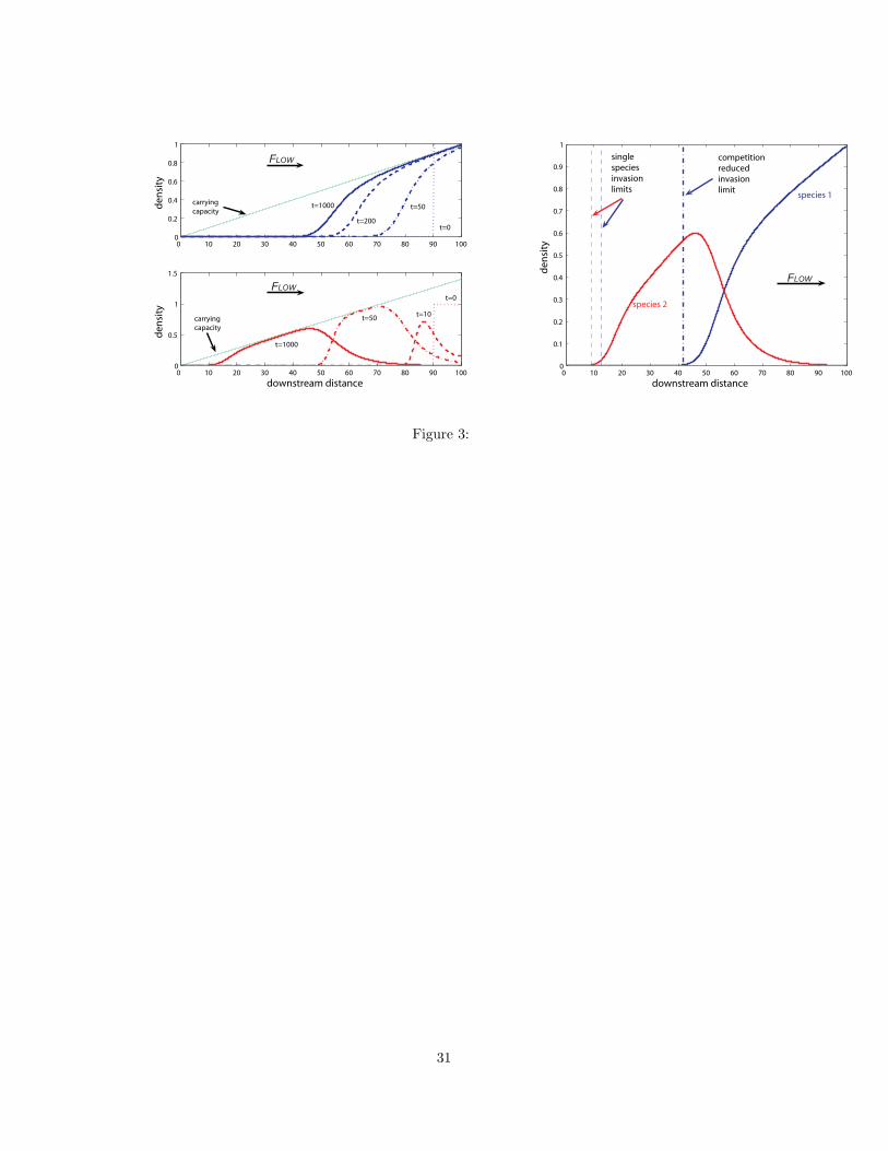
Figure 3 shows the resulting behavior of the two competing species under such heteroge-

neous environmental conditions. Initially, both species are located downstream. The weaker

competitor develops a fast moving front that stalls at its invasion limit, x#2, as in the sin-

gle species case. Downstream, the better competitor drives the weaker one to extinction

and slowly moves upstream in a monotone wave. This wave stalls far downstream from the

single-species invasion limit, x#1, namely at the competition-reduced invasion limit, x##1 . At

the resulting steady state, there is a spatial zone of coexistence of the two species. In contrast

to the coexistence zone in the homogeneous environment above, this zone is not a boundary

e!ect but occurs around the reduced invasion limit of species 1. To summarize:

1. Species 2 spreads upstream in form of a wave that stalls at the invasion limit x#2.

2. Species 1 does not reach its invasion limit x#1 but only reaches the reduced limit x##1 .

The question of what controls the steepness of the transitions between the states becomes

more di"cult to answer in this case since more locations and parameters are involved. We

concentrate on the front of species 1, where we vary parameters in such a way as to fix the

invasion limit x##1 . For increasing D (and therefore decreasing R) the front becomes less steep.

Varying the gradient of R while keeping D fixed has no visible e!ect on the steepness of the

front.

4 Discussion

By integrating local growth and interaction with longitudinal transport and di!usion, we

identify a novel approach to understanding processes and patterns in stream ecology. We

illustrate this approach using a simple model for one single or two competing species. The

major results are the emergence of an upstream invasion limit of a species and two mechanisms

of coexistence of competitors along the spatial domain.

13

Invasion Limits and Stalled Waves

The model not only predicts under which conditions on di!usion, flow and growth rates a

species can persist in a certain stream reach as was done before (Speirs and Gurney, 2001;

Pachepsky et al., 2005), but it also predicts the location of the upstream limit where a species

can persist in a heterogeneous environment. This limit is defined formally as the spatial

location where the upstream invasion speed in a corresponding homogeneous environment

is zero. Numerical simulations reveal that at this limit there is a sharp transition from

almost zero to high density that emerges from a stalled wave. Analytical investigations on

the steepness of the transition and the rate at which zero and the positive steady state

are approached spatially are currently underway. Since the model is based on the di!usion

equation, the steady state is everywhere positive unless it is identically zero. For ecological

purposes, however, the density above the invasion limit is e!ectively zero.

Our model explicitly considers how colonization and local processes combine to produce

spatial dynamics. There are few studies that consider “open systems” (Nisbet et al., 1997)

and even fewer that explicitly consider the importance of a colonizer pool (Stevenson and

Peterson, 1991). While the idea of an upstream invasion might sound strange at first, given

that species such as algae and invertebrates are subject to water currents, we want to point

out that advection-di!usion equations appear to capture the process of particle transport in

flow environments reasonably well (Bencala and Walters, 1983).

Coexistence Mechanisms

The analysis of the spatial Lotka-Volterra competition model in homogeneous and hetero-

geneous environments reveals two inherently spatial mechanisms for coexistence in the case

where the competition coe"cients indicate competitive exclusion in the corresponding non-

spatial system. As in the previous section, we always refer to species 1 as the better com-

14

petitor whereas species 2 has the higher growth rate.

The first mechanism occurs in the homogeneous environment and is identified as a bound-

ary e!ect. The flow at the upstream boundary pushes both competitors downstream and

decreases their density near the boundary. The small density of species 1 has only a small

e!ect on species 2. This boundary layer is small for small flow velocities so that species 1

still excludes species 2. For intermediate velocities, however, species 2 can coexist at the

upstream boundary, and for higher velocities the competitive outcome is even reversed so

that species 2 alone persists. Conversely, this suggests that decreasing flow rates, e.g. due

to water extraction, may lead to changes in species composition through upstream invasion

of superior competitors. This e!ect may be compounded by concomitant changes in nutri-

ent concentration with decreased flow rate. Potapov and Lewis (2004) present an in-depth

analysis of similar phenomena in the context of population spread under climate shift.

This boundary e!ect described above depends on the presence of flow and is therefore

di!erent from previously established results where di!usion induced boundary loss facilitates

coexistence (Fagan et al., 1999).

The second mechanism for coexistence occurs in heterogeneous environments where the

growth rate increases downstream. This is a common feature in many river systems where

nutrient load and/or temperature, which limit primary production upstream, increase down-

stream. This heterogeneity creates an upstream invasion limit where the invasion wave of a

single species is stalled. Since species 2 has its invasion limit upstream of that of species 1,

it is able to establish there. Because the weaker competitor (species 2) becomes established

further upstream, it has the advantage of a pool of potential colonizers upstream of the dom-

inant competitor (species 1). Downstream of this colonizer pool of species 2, flow removes

individuals of both species but delivers only colonizers of species 2. The combined result of

these processes is that the competitive superiority of species 1 is lost in some region down-

15

stream. Species 1 is not able to persist at its single-species invasion limit but only further

downstream at the invasion limit predicted with the competitor at carrying capacity.

This second mechanisms depends on the gradient of the growth rate and is clearly not a

boundary e!ect. It creates spatial areas dominated by only one species and some transition

zone in between. Depending on the flow velocity and the steepness of the gradient in growth

rate, this coexistence zone can vary in size. Ballyk et al. (1998) modeled resource-mediated

competition in a plug-flow reactor and found parameter regimes of spatially-mediated coex-

istence. Whereas the resource in their model is supplied at the top end of the reactor and

decreases downstream, we consider the case where the growth rate increases downstream.

Cantrell and Cosner (1998) showed how spatially varying growth and interaction rates in a

di!usive Lotka-Volterra system can create spatial segregation of competitors and thereby fa-

cilitate coexistence. Again, the mechanism here is induced by the advective flow and therefore

fundamentally di!erent from the pure di!usive system.

Spatial Scales

Above, we described several possible mechanisms that lead to spatial patterns in population

distribution. Our initial investigation was general with respect to the parameter values.

Now we explore the spatial scales at which we expect to observe these patterns for realistic

parameter values.

Typical growth rates of periphyton (benthic algae) range 0.1–2d!1 (DeAngelis et al.,

1995; Son and Fujino, 2003). Di!usion rates of 0.1–0.5m2s!1, and average flow speeds of

0.01–0.03ms!1 were obtained from fitting advection-di!usion equations to data from conser-

vative tracer injection experiments (Bencala and Walters, 1983; Kim et al., 1992). Speirs

and Gurney (2001) already concluded for their model that populations cannot persist in a

well-mixed water column when individuals are assumed to experience the average flow speed.

However, most planktonic or invertebrate species in rivers are not purely pelagic but have

16

benthic stages (Allan, 1995). In that case, the e!ective flow speed experienced by the pop-

ulation is reduced considerably. First, the flow speed is much reduced near the benthos.

According to formula (13) by Speirs and Gurney (2001), the flow speed in the lowest 4% of

the river depth is only 10% of the average flow speed. Secondly, relative abundance estimates

of benthic and flow populations indicate that for some species individuals spend only as little

as 0.01% of the time in the flow (Speirs and Gurney, 2001). When individuals are exposed

to the flow only for a fraction of the time, then the e!ective flow speed that these individuals

experience is reduced by the same factor, i.e., by approximately 10!4. Pachepsky et al. (2005)

have modeled this transition between benthic and pelagic stages explicitly.

The invasion condition requires that the e!ective flow speed be bounded by

Ve! % 2$

DR & 6.8 · 10!4 " 6.8 · 10!3 m s!1 = 0.058" 0.58 km d!1.

This requires an e!ective flow speed that is 10–100 fold lower than the average flow speed of

0.01–0.03ms!1. This reduction clearly falls in the range discussed above.

At first, we turn to the width of the transition zone at the upstream invasion limit for

a single species as illustrated in Figure 1. Setting D = 0.1 m2 s!1 to its lowest value, we

set the growth rate to vary R = 0.1 " 0.3 d!1 over a spatial scale of 100 km. An average

e!ective flow speed of V = 10!3 ms!1 puts the invasion limit at x# = 58 km (10). The

steady state distribution increases from zero to R over a region of 4 km near the invasion

limit. Doubling D and reducing R to half its value leaves the invasion limit unchanged but

widens the transition zone to a 6 km region.

Next, we look at the case of boundary coexistence. We fix D = 0.1 m2 s!1 as above and

set R = 0.2 d!1. The interaction coe"cients are as in section 3. For flow speeds smaller than

2 · 10!4 ms!1, species 1 outcompetes species 2. At flow speeds above 7 · 10!4 ms!1 species

2 takes over and species 1 goes extinct. In between, both species are present in a range of

5–10 km below the upstream boundary.

17

Finally, we examine the size of the coexistence region in a heterogeneous habitat. We fix

a flow speed of V = 10!3 ms!1. Interaction coe"cients are as in section 3. We set up the

di!usion rate and the variation in growth rates over a stream reach of 100 km in such a way

that the weaker competitor can invade all the way to the top of the stream and the reduced

invasion limit for the superior competitor lies in the 0–100 km region of space. For D = 0.1

m2 s!1 and a range of R = 0.3" 0.9 d!1 the coexistence zone extends approximately 10 km.

Increasing di!usion to D = 0.3 m2 s!1 while reducing growth to R = 0.2" 0.4 d!1 expands

the coexistence region to nearly 20 km. For even higher di!usion of D = 0.5 m2 s!1 and

lower growth R = 0.1 " 0.2 d!1, together with increased # = 1.45 the coexistence region

spans almost 50 km.

These examples demonstrate that the mechanisms presented above, and illustrated in

Figures 1–3, can produce patterns on relevant scales of several hundred meters to tens of

kilometers. We want to note that the di!usion rates used above only reflect the physical

conditions in the flow. We conjecture that biological processes such as grazing and movement

by grazers can produce a larger e!ective di!usion rate, which in turn has the potential to

increase the coexistence regions to the order of hundreds of kilometers. Future work will also

focus on the e!ect of the competition coe"cients on these patterns.

Extensions

We chose the Lotka-Volterra equations as the simplest representation of competitive interac-

tions. In reality, these interactions are often mediated though resources, which follow their

own dynamics. We recognize the importance of this complexity and plan to incorporate more

mechanistic descriptions of competitive processes (e.g. light and nutrient-based algal growth)

in future work. Similarly, it will be necessary to compare the results obtained here to mod-

els that incorporate more explicit environmental properties of rivers (e.g. hydraulic features

(pool-ri#e structures), storage zones, spatially-explicit nutrient perturbations (point-source

18

versus non-point source inputs)).

Whereas we focused the model and discussion on riverine systems, they may apply to

terrestrial systems as well. For example, Potapov and Lewis (2004) use a similar model

to study the impact of moving temperature isoclines on competitors. More generally, the

coexistence of two or more competitors on a few limiting resources has been and still is a

very active field in spatial ecology (Lehmann and Tilman, 1997). The most widely accepted

explanation for this paradox is an assumed trade-o! between competition and colonization,

where frequently colonization ability is related to dispersal ability (Lehmann and Tilman,

1997), for example via seed size (Levin and Muller-Landau, 2000).

In contrast to this, both competitors in our system have exactly the same dispersal ability,

indicating that colonization should be thought of as the combination of two processes, namely

dispersal ability and growth rate at low density. We conjecture that by allowing the di!usion

rates and/or flow speeds to vary between the species, the e!ects observed above can change in

spatial extend, and new e!ects may appear as in Potapov and Lewis (2004). Di!usion as well

as e!ective flow speed are partly determined by the dynamics of the water (e.g. turbulence,

flow) and partly by behavioral factors (e.g. active dispersal, adherence to benthos). Benthic

stages have been incorporated into single-species models for river ecosystems (Lutscher et al.,

2005; Pachepsky et al., 2005), and it is part of our ongoing research e!orts to explore the

e!ects of these stages on competitive systems.

We have concentrated on the spatial mechanisms by which coexistence or competitive

reversal can be achieved from a case where the non-spatial model predicts competitive exclu-

sion. We conjecture that the results qualitatively still hold when we replace Lotka-Volterra

competition with resource-mediated competition. These models typically predict competitive

exclusion as the only outcome in a non-spatial setting (Smith and Waltman, 1995). The non-

spatial Lotka-Volterra model also predicts coexistence and founder control in certain regions

19

of parameter space. Future work will assess the e!ect of di!usion and flow on these outcomes.

Neuhauser and Pacala (1999) have shown in a stochastic interacting-particle system that both

these regions in parameter space may decrease in size in favor of competitive exclusion when

symmetric dispersal is considered. We speculate that in systems with advection, new e!ects

will appear. It may be possible that the “founder control”-scenario becomes and “upstream

control”-scenario, in which the species that invades further upstream dominates the other.

5 Acknowledgements

The authors thank C. Cosner and H.L. Smith for inspiring discussions. FL gratefully acknowl-

edges support as a PIMS postdoctoral fellow. EM acknowledges support from NSERC and

the Canada Research Chair Program. This research was also supported by grants from the

NSERC Clean Water Network and the Alberta Ingenuity Centre for Water Research. MAL

gratefully acknowledges support from NSERC Discovery and CRO grants and a Canada Re-

search Chair.

20

References

Allan, J. (1995). Stream Ecology: structure and function of running waters. Chapman &

Hall, London.

Alvarez, M. and Peckarsky, B. (2005). How do grazers a!ect periphyton heterogeneity in

streams? Oecologia, 142(4), 576–587.

Amarasekare, P., Hoopes, M., Mouquet, N., and Holyoak, M. (2004). Mechanisms of coexis-

tence in competitive metacommunities. Am. Nat., 164(3), 310–326.

Ballyk, M. and Smith, H. (1999). A model of microbial growth in a plug flow reactor with

wall attachment. Math. Biosci., 158, 95–126.

Ballyk, M., Dung, L., Jones, D. A., and Smith, H. (1998). E!ects of random motility on

microbial growth and competition in a flow reactor. SIAM J. Appl. Math., 59(2), 573–596.

Bencala, K. and Walters, R. (1983). Simulation of solute transport in a mountain pool-and-

ri#e stream: A transient storage model. Water Resources Res., 19(3), 718–724.

Biggs, B., Goring, D., and Nikora, V. (1998). Subsidy and stress responses of stream peri-

phyton to gradients in water velocity as a function of community growth form. J. Phycol.,

34, 598–607.

Britton, N. F. (2003). Essential Mathematical Biology. Springer, London

Cantrell, R. S. and Cosner, C. (1998). On the e!ects of spatial heterogeneity on the persis-

tence of interacting species. J. Math. Biol., 37, 103–145.

Cardinale, B., Palmer, M., Ives, A., and Brooks, S. (2005). Diversity-productivity relation-

ships in streams vary as a function of the natural disturbance regime. Ecology, 86(3),

716–726.

21

DeAngelis, D., Loreau, M., Neergaard, D., Mulholland, P., and Marzolf, E. (1995). Mod-

elling nutrient-periphyton dynamics in streams: the importance of transient storage zones.

Ecol. Modelling, 80, 149–160.

Dent, L., Cumming, G., and Carpenter, S. (2002). Multiple states in river and lake ecosys-

tems. Philosophical Transactions: Biological Sciences, 357, 635–645.

Fagan, W. F., Cantrell, R. S., and Cosner, C. (1999). How habitat edges change species

interaction. Am. Nat., 153, 165–182.

Fisher, R. (1937). The advance of advantageous genes. Ann. Eugenics, 7, 355–369.

Fisher, S., Grimm, N., Marti, E., Holmes, R., and Jones, J. J. (1998). Material spiralling in

stream corridors: a telescoping ecosystem model. Ecosystems, 1, 19–34.

Flipo, N., Even, S., Poulin, M., Tusseau-Vuillemin, M.-H., Ameziane, T., and Dauta, A.

(2004). Biogeochemical modelling at the river scale: plankton and periphyton dynamics,

Grand Morin case study, France. Ecol. Modelling, 176, 333–347.

Gaylord, B. and Gaines, S. (2000). Temperature or Transport? Range limits in marine

species mediated solely by flow. Am. Nat., 155, 769–789.

Henry, J. and Fisher, S. (2003). Spatial segregation of periphyton communities in a desert

stream: Causes and consequences for N cycling. Journal of the North American Bentho-

logical Society, 22(4), 511–527.

Hill, B., Herlihy, A., Kaufmann, P., Stevenson, R., and McCormick, F. (2000). Use of

periphyton assemblage data as an index of biotic integrity. Journal of the North American

Benthological Society, 19(1), 50–67.

Hillebrand, H. (2002). Top-down versus bottom-up control of autotrophic biomass: A meta-

22

analysis on experiments with periphyton. Journal of the North American Benthological

Society, 21(3), 349–369.

Kim, B., Jackman, A., and Triska, F. (1992). Modeling biotic uptake by periphyton and

transient hyporrheic storage of nitrate in a natural stream. Water Resources Res., 28,

2743–2752.

Lamberti, G., Gregory, S., Ashkenas, L., Steinman, A., and McIntire, C. (1989). Productive

capacity of periphyton as a determinant of plant-herbivore interactions in streams. Ecology,

70(6), 1840–1856.

Lavoie, I., Warwick, F., Reinhard, P., and Painchaud, J. (2003). E!et du debit sur la

dynamique temporelle des algues periphytiques dans une riviere influencee par les activites

agricoles. Revue des Sciences de l’Eau, 16(1), 55–77.

Lehmann, C. and Tilman, D. (1997). Competition in spatial habitats. In D. Tilman and

P. Kareiva, editors, Spatial Ecology, volume 30 of Monographs in Population Biology, pages

185–203. Princeton University Press.

Leopold, L. (1962). Rivers. Am. Sci., 50, 511–537.

Levin, S. and Muller-Landau, H. (2000). The evolution of dispersal and seed size in plant

communities. Evol. Ecol. Res., 2, 409–435.

Lewis, M., Li, B., and Weinberger, H. F. (2002). Spreading speed and linear determinacy for

two-species competition models. J. Math. Biol., 45, 219–233.

Lutscher, F., Pachepsky, E., and Lewis, M. (2005). The e!ect of dispersal patterns on stream

populations. SIAM Appl. Math, 65(4), 1305–1327.

Lutscher, F., Lewis, M., and McCauley, E. (in press). The e!ects of heterogeneity on popu-

lation persistence and invasion in rivers. Bull. Math. Biol.

23

McCormick, P. V. and Stevenson, R. (1991). Mechanisms of benthic algal succession in lotic

environments. Ecology, 72(5), 1835–1848.

McIntire, C., Gregory, S., Steinman, A., and Lamberti, G. (1996). Modeling benthic algal

communities: An example from stream ecology. In R. Stevenson, M. Bothwell, and R. Lowe,

editors, Algal Ecology: Freshwater benthic ecosystems. Academic Press.

Mulholland, P. and DeAngelis, D. (2000). Surface-subsurface exchange and nutrient spiraling.

In J. Jones Jr. and P. Mulholland, editors, Streams and Ground Waters, pages 149–166.

Academic Press, New York.

Muller, K. (1982). The colonization cycle of freshwater insects. Oecologica, 53, 202–207.

Murray, J.D. and Sperb, R.P. (1983) Minimum domains for spatial patterns in a class of

reation di!usion equations. J. Math. Biol., 18, 169–184.

Neuhauser, C. and Pacala, S. (1999). An explicitly spatial version of the Lotka-Volterra

model with interspecific competition. Ann. Appl. Prob., 9(4), 1226–1259.

Nisbet, R., Diehl, S., Wilson, W., Cooper, S., Donalson, D., and Kratz, K. (1997). Primary-

productivity gradients and short-term population dynamics in open systems. Ecol. Mono-

graphs, 67(4), 535–553.

Pachepsky, E., Lutscher, F., Nisbet, R., and Lewis, M. A. (2005). Persistence, spread and

the drift paradox. Theor. Pop. Biol., 67, 61–73.

Peterson, C. and Stevenson, R. (1992). Resistance and resilience of lotic algal communities

- Importance of disturbance timing and current. Ecology, 73(4), 1445–1461.

Peterson, C. G. (1996). Mechanisms of lotic microalgal colonization following space-clearing

disturbances at di!erent spatial scales. Oikos, 77, 417–435.

24

Potapov, A. and Lewis, M. (2004). Climate and competition: The e!ect of moving range

boundaries on habitat invasibility. Bull. Math. Biol., 66(5), 975–1008.

Pringle, C. (1990). Nutrient spatial heterogeneity: E!ects on community structure, physiog-

nomy, and diversity of stream algae. Ecology, 71, 905–920.

Robinson, C. and Minshall, G. (1986). E!ects of disturbance frequency on stream benthic

community structure in relation to canopy cover and season. Journal of the North American

Benthological Society, 5(3), 237–248.

Shigesada, N. and Kawasaki, K. and Teramoto, E. (1986) Traveling Periodic Waves in

Heterogeneous Environments. Theor. Popul. Biol., 30, 143–160.

Smith, H. (1995). Monotone Dynamical Systems. America Mathematical Society.

Smith, H. and Waltman, P. (1995). The Theory of the Chemostat: Dynamics of Microbial

Competition. Cambridge University Press, New York.

Snyder, E., Robinson, C., Minshall, G., and Rushforth, S. (2002). Regional patterns in

periphyton accural and diatom assemblage structure in a heterogeneous nutrient landscape.

Canadian Journal of Fisheries and Aquatic Sciences, 59, 564–577.

Son, D. and Fujino, T. (2003). Modeling approach to periphyton and nutrient interaction in

a stream. J. Enviro. Eng., 129(9), 834–843.

Speirs, D. and Gurney, W. (2001). Population persistence in rivers and estuaries. Ecology,

82(5), 1219–1237.

Stevenson, R. and Peterson, C. (1991). Emigration and immigration can be important de-

terminants of benthic diatom assemblages. Freshwater Biology, 26, 279–294.

Strickwerda, J. (1989) Finite di!erence schemes and partial di!erential equations. Chapman

& Hall, New York

25

Vannote, R., Minshall, G., Cummins, K., Sedell, J., and Cushing, C. (1980). The river

continuum concept. Can. J. Fish. Aquat. Sci., 37, 130–137.

Ward, J. and Stanford, J. (1983). The serial discontinuity concept of lotic ecosystems. In

T. Fontaine and S. Bartell, editors, Dynamics of lotic ecosystems, pages 29–42, Ann Arbor,

Michigan. Ann Arbor Science Publications.

Woodward, G. and Hildrew, A. (2002). Food web structure in riverine landscapes. Freshwater

Biology, 47, 777–798.

Wright, K. and Li, J. (2002). From continua to patches: Examining stream community

structure over large environmental gradients. Canadian Journal of Fisheries and Aquatic

Sciences, 59(8), 1404–1417.

26

Figures and Table

Legend for Figure 1

Invasion process and steady state for a single species in a resource gradient. The flow is from

left to right. The initial density (t = 0) is located downstream. The profile of the invasion

front is plotted every 100 time units. As the front approaches the invasion limit x# = 21

(10), it slows down until it comes to a halt. Upstream the density is almost zero, downstream

the density is almost the carrying capacity. The transition between the two states is very

steep, much steeper than the gradient in the carrying capacity. The unscaled parameters are

L = 100, D = 1, RU = 1, RL = 2, V = 2.2. In the plot, the densities are scaled to unity.

Legend for Figure 2

Time evolution and steady states for two competing species in a homogeneous environment.

Initially, both competitors occupy the downstream half of the domain at equal density, but

the final outcome is independent of the initial values as long as both species are present.

The upper left panels show how within the first 50 time units, species 2 forms an upstream

moving front whereas species 1 outcompetes species 2 downstream. The panel on the right

shows how subsequently species 1 invades upstream, but much slower than species 2 initially.

The third panel on the bottom shows steady state distributions for the two species for two

di!erent values of flow speeds where coexistence is possible. For larger flow speed, species

2 occupies more space (solid line). The parameters are L = 100, D = 1, RU = RL = 1, # =

1.4, A11 = A22 = 1, A12 = 0.5, A21 = 1.5. The larger flow speed if V = 1.2 (also upper

panels), the smaller one is V = 0.8.

27

Legend for Figure 3

Invasion of two competitors as in Figure 2 but in an environment with resource gradient sim-

ilar to Figure 1. The two panels on the left show how the two species spread upstream

from their initial downstream location. As in Figure 2, the weaker competitor spreads

much faster initially, and the better competitor takes a long time to invade and partially

replace its opponent. These two di!erent time scales are reflected in the times chosen to

plot the densities. The steady state in the right panel shows that even though the single-

species invasion limits are close together, only the weaker competitor can become established

upstream. The better competitor reaches its reduced invasion limit. The parameters are

L = 100, D = 1, RU = 0, RL = 2, # = 1.4, V = 1, and competition parameters as above.

Legend for Table 1

Modeling approaches for periphyton. In each category we only list the most recent reference

for the model type or author group. All models contain population dynamics of periphyton

and are parameterized from experiments. Flow is included as an additional loss term. Only

the model by Stevenson and Peterson (1991) considers emigration and immigration explicitly,

none of the others contains spatial movement of periphyton. The models by McIntire et al.

(1996) and Stevenson and Peterson (1991) are non-spatial, Mulholland and DeAngelis (2000)

and Son and Fujino (2003) consider both, nonspatial and spatial models, the approach by

Flipo et al. (2004) is explicitly spatial and, as the only one in the list, includes hydrodynamics.

28

Figure 1:

29

0 10 20 30 40 50 60 70 80 90 1000

0.2

0.4

0.6

0.8

1

de

nsi

ty

0 10 20 30 40 50 60 70 80 90 1000

0.5

1

1.5

downstream distance

de

nsi

ty

t=0

t=0

t=10

t=20

t=50

t=10

t=50

0 10 20 30 40 50 60 70 80 90 1000

0.2

0.4

0.6

0.8

1

de

nsi

ty

0 10 20 30 40 50 60 70 80 90 1000

0.5

1

1.5

downstream distanced

en

sity

t=100

t=100

t=200

t=300

t=!

t=200

t=300

t=!

0 10 20 30 40 50 60 70 80 90 1000

0.2

0.4

0.6

0.8

1

1.2

1.4

distance downstream

de

nsi

ty

FLOW

v small

v large

Species 1

species 2

Figure 2:

30

0 10 20 30 40 50 60 70 80 90 1000

0.2

0.4

0.6

0.8

1

de

nsi

ty

0 10 20 30 40 50 60 70 80 90 1000

0.5

1

1.5

downstream distance

de

nsi

ty

t=0

t=50

t=200t=0

t=50

t=1000

t=10

t=1000

carryingcapacity

carryingcapacity

0 10 20 30 40 50 60 70 80 90 1000

0.1

0.2

0.3

0.4

0.5

0.6

0.7

0.8

0.9

1

downstream distance

de

nsi

ty

singlespeciesinvasionlimits

competitionreducedinvasionlimit

species 1

species 2

FLOW

FLOWFLOW

Figure 3:

31