Space Curves and the “TNB-Frame” These notes discuss the set of unit vectors associated with a space curve r ( t ) , the planes defined by those vectors, and the curvature at a point on the curve, as illustrated by a specific example. The curve used here is described in Problem 43 of Section 13.3 in Stewart (6th edition, p. 837). We are to investigate the curve described by the vector function

€

r r ( t ) = < t 2, 23 t 3 , t > at the point P

€

(1 , 23 , 1) . We can see immediately that the

value of the parameter at this point must be t = 1 . For many of the calculations we will be making later, it is useful to have the derivative of the vector function for the curve, which is found by differentiating the individual coordinate functions with respect to the parameter t :

€

r r ( t ) = < f ( t ) , g( t ) , h( t ) >

€

→r r ' ( t ) = < d

dt f ( t ) , ddt g( t ) , d

dt h( t ) >

€

= < ddt ( t

2 ) , ddt (

23 t

3 ) , ddt ( t ) > = < 2t , 2t 2 , 1> .

At the point P , then, the derivative vector is

€

r r ' (1) = < 2 ⋅1 , 2 ⋅12 , 1> = < 2 , 2 , 1> ,

which has a length of

€

r r ' (1) = 22 + 22 + 12 = 3 . It is common practice to describe

the way in which the direction of the space curve is changing as t advances by using a unit vector defined by the derivative vector divided by its length; this is called the (unit) tangent vector T ( t ) . So, at point P ,

€

r T ( t ) * =

r r ' ( t )r r ' ( t )

⇒r

T (1) =r r ' (1)r r ' (1)

=< 2 , 2 , 1>

3or < 2

3 ,23 ,

13 > .

* To make it clear that this is a unit vector, many people write it as

€

ˆ T ( t ) . (If we had need of the general function for the tangent vector for this curve, we would calculate

€

r r ' ( t ) = (2t )2 + (2t 2 )2 + 12 = 4t 2 + 4t 4 + 1

€

= (2t 2 + 1)2 = 2t 2 + 1 and

€

r T ( t ) =

< 2t , 2t 2 , 1>

2t 2 + 1or < 2t

2t 2 + 1, 2t 22t 2 + 1

, 12t 2 + 1

> . )

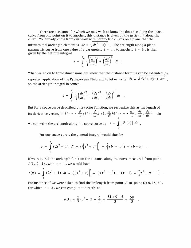
There are occasions for which we may wish to know the distance along the space curve from one point on it to another; this distance is given by the arclength along the curve. We already know from our work with parametric curves on a plane that the

infinitesimal arclength element is

€

ds = dx 2 + dy 2 . The arclength along a plane

parametric curve from one value of a parameter, t = a , to another, t = b , is then given by the definite integral

€

s = dxdt⎛ ⎝ ⎜ ⎞

⎠ ⎟ 2

+dydt

⎛ ⎝ ⎜

⎞ ⎠ ⎟ 2

a

b

∫ dt .

When we go on to three dimensions, we know that the distance formula can be extended (by

repeated application of the Pythagorean Theorem) to let us write

€

ds = dx 2 + dy 2 + dz 2 ,

so the arclength integral becomes

€

s = dxdt⎛ ⎝ ⎜ ⎞

⎠ ⎟ 2

+dydt

⎛ ⎝ ⎜

⎞ ⎠ ⎟ 2

+ dzdt⎛ ⎝ ⎜ ⎞

⎠ ⎟ 2

a

b

∫ dt .

But for a space curve described by a vector function, we recognize this as the length of

its derivative vector,

€

r r ' ( t ) = < ddt f ( t ) , d

dt g( t ) , ddt h( t ) > = < dx

dt ,dydt ,

dzdt > . So

we can write the arclength along the space curve as

€

s =r r ' ( t )

a

b

∫ dt .

For our space curve, the general integral would thus be

€

s = (2t 2 + 1)a

b

∫ dt = ( 23 t3 + t )

a

b= 2

3 (b3 − a3) + (b − a ) .

If we required the arclength function for distance along the curve measured from point

P

€

(1 , 23 , 1) , with t = 1 , we would have

€

s(τ ) = (2t 2 + 1)1

τ

∫ dt = ( 23 t3 + t )

1

τ= 2

3 (τ3 − 13) + (τ − 1) = 2

3τ3 + τ − 5

3 .

For instance, if we were asked to find the arclength from point P to point Q ( 9, 18, 3 ) ,

for which t = 3 , we can compute it directly as

€

s(3) = 23 ⋅ 3

3 + 3 − 53 =

54 + 9 − 53 = 58

3 .

One way in which the concept of arclength of a curve is helpful is in describing properties of the curve which are independent of the coordinate system that is used; such properties of the curve itself are called “intrinsic”. An intrinsic property which is often of interest is the rate at which the unit tangent vector T ( t ) changes as, say, a particle progresses along the curve at a constant speed. A situation where people encounter arclength is in the marked distances on a highway: the mile-markers and signs indicating distances to destinations refer to distances which must be traveled along the road. (Generally then, the distance shown to travel from one city to another is longer than the straight-line distance between those cities.) The curve which the highway follows can be said to be marked off using an “arclength parameterization”. So where a motorist’s speedometer shows that their car is moving at a constant speed, we could say that they are covering the arclength s

between two locations at a constant rate

€

dsdt .

We can continue this analogy and consider what happens when the motorist encounters a turn in the road (anything from a gentle change in direction to taking a looping exit ramp). The unit tangent vector T ( t ) points in the direction that the car is moving at a given instant. As long as the road is straight, this vector does not change. When the path makes a curve, the vector T ( t ) changes direction, slowly for a gentle turn, much more rapidly for an exit loop. We can define a quantity which relates the change in the direction of T ( t ) to the change in distance being traveled along the

road; it is called “curvature” and is calculated as

€

κ =d

r T

ds .

As it stands, this ratio is not very convenient to compute, since we would need to work out an arclength parameterization for our curve, express the tangent vector as T ( s ) , and then find the necessary derivative. But upon referring back to what we’ve learned about using the Chain Rule for finding derivatives of parameteric curves (Chapter 10 in Stewart) , we know that if variables x and y are both functions of a

parameter t , we can calculate a derivative as

€

dydx

=dy dtdx dt

. So we could make the

curvature calculation as

€

κ =d

r T dt

ds dt ; this would still require us to work out that

arclength parameterization for the curve, though. As it happens, there is one other simplification we can make: since the arclength function for the curve is defined by the

integral

€

s(τ ) =r r ' ( t )

a

τ

∫ dt , the Fundamental Theorem of (Integral) Calculus tells

us that (at least for differentiable functions) the derivative of the integral function (here,

the arclength function) is just the function being integrated. Thus,

€

dsdt =

r r ' ( t ) ,

which means that we can now write

€

κ ( t ) =d

r T dt

d r r dtor

r T ' ( t )r r ' ( t )

.

An alternate expression which is sometimes easier to apply in calculations, depending on the complexity of the vector function for the curve, r ( t ) , can be derived from properties of the vectors r ( t ) and T ( t ) as

€

κ ( t ) =r r ' ( t ) × r r ' ' ( t )

r r ' ( t ) 3.

(A proof is provided in Stewart, p. 833.)

To return to our space curve,

€

r r ( t ) = < t 2, 23 t 3 , t > , it is about the same

amount of effort to calculate the curvature using either formula. For the first, we must work out the derivative

€

r T ' ( t ) =

ddt

< 2t2t 2 + 1

, 2t 22t 2 + 1

, 12t 2 + 1

> = < ddt

2t2t 2 + 1⎛

⎝ ⎜

⎞

⎠ ⎟ ,

ddt

2t 22t 2 + 1⎛

⎝ ⎜

⎞

⎠ ⎟ , d

dt1

2t 2 + 1⎛

⎝ ⎜

⎞

⎠ ⎟ >

€

= <2 − 4t 2

2t 2 + 1⎛ ⎝ ⎜ ⎞

⎠ ⎟ 2 ,

4t2t 2 + 1( )2

, − 4 t

2t 2 + 1( )2>   ,

for which we would then determine its length. For the other formula, the second

derivative

€

r r ' ' ( t ) = ddt < 2t , 2t 2 , 1> = < 2 , 4t , 0 > is easy enough to compute, but

then we must calculate a cross product vector and find its length. By either means, we arrive at the result

€

κ ( t ) =16t 4 + 16t 2 + 4(2t 2 + 1)3

=2 4 t 4 + 4 t 2 + 1

(2t 2 + 1)3=2 (2t 2 + 1)2

(2t 2 + 1)3=

2(2t 2 + 1)2

.

At point P

€

(1 , 23 , 1) , the curvature is then

€

κ (1) =2

(2 ⋅12 + 1)2= 232

= 29 .

We can further characterize the behavior of a space curve as it bends. When a

unit vector

€

ˆ v changes its direction, its derivative

€

ˆ v ' is perpendicular to

€

ˆ v . So we define a unit vector which describes the change in the unit tangent vector T ( t ) , called

the (unit) normal vector

€

r N ( t ) =

r T ' ( t )r

T ' ( t )[also written as ˆ N ( t ) ] . For our space

curve, we can now quickly determine that

€

r N ( t ) =

<2 − 4 t2

2t2+ 1⎛ ⎝ ⎜ ⎞

⎠ ⎟ 2, 4 t

2t2+ 1( )2,

− 4 t

2t2+ 1( )2>

2

2t2+ 1( )= <

1− 2t 22t 2 + 1

, 2t2t 2 + 1

, − 2t2t 2 + 1

> and

€

r N (1) = <

1− 2 ⋅122 ⋅12 + 1

, 2 ⋅12 ⋅12 + 1

, − 2 ⋅12 ⋅12 + 1

> = < − 13 ,23 , −

23 > .

We are now able to bring together what we have developed so far to describe some additional properties of the space curve. The tangent vector T ( t ) and the normal vector N ( t ) define a plane at each point along the curve called the “osculating plane”. At any point, the plane there contains a circle referred to as the “osculating circle” which touches the curve at that point and has a curvature which matches that of the space curve there. If we take the parametric description for a circle with radius R , centered at the origin, which is x ( t ) = R cos ωt , y ( t ) = R sin ωt , we can use the definitions we’ve

discussed above to show that the curvature of this circle is a constant

€

κ = 1R . For a

space curve, the curvature can vary from point to point, so we usually define the radius

of the osculating circle at each point with the function

€

ρ( t ) = 1κ ( t ) (“the tighter the

turn, the smaller the radius and the larger the curvature”). The normal vector at a point on the curve points in the direction of the center of the osculating circle (we could say that “ N ( t ) points at the center of the turn”). For our particular space curve, the radius of the osculating circle is therefore

€

ρ( t ) = 1κ ( t ) = 1

2( 2t2 + 1 )2

⎡

⎣

⎢ ⎢

⎤

⎦

⎥ ⎥

=(2t 2 + 1)2

2 . At the point P

€

(1 , 23 , 1) , this is

€

ρ(1) = 1κ (1) = 1

29⎛

⎝ ⎜

⎞

⎠ ⎟

=92 . The center of the osculating circle lies on a line which has a

direction given by

€

ˆ N (1) = < − 13 , 2

3 , − 23 > and passes through the point P . This line

then has the parametric equations

€

x = 1 − 13 t , y = 2

3 + 23 t , z = 1 − 2

3 t . Since N ( t ) is a unit vector, the center of the circle is found at the location on this line specified by t = ρ ( 1 ) , placing its coordinates at

€

x = 1 − 13 ⋅92 = − 12 , y = 2

3 + 23 ⋅92 = 11

3 , z = 1 − 23 ⋅92 = − 2 .

We may recall from Chapter 12 in Stewart that if we know two vectors which define a plane, we can find an equation for the plane in space if we know a vector perpendicular to the plane. (Unfortunately, in the context of these notes, this is known as the normal vector to the plane, which is denoted by n . We will be careful to distinguish this from the normal vector N ( t ) at a point of the space curve.) Since the two vectors lie in the plane, the normal vector to the plane is also perpendicular to both of these vectors. A vector perpendicular to two vectors can be found by calculating their cross product vector. We found that if the plane contains a point ( x

0, y

0, z

0 ) and

has the normal vector n = < a , b , c > , the equation for the plane is given by a · ( x – x

0 ) + b · ( y – y

0 ) + c · ( z – z

0 ) = 0 .

The osculating plane contains the vectors T ( t ) and N ( t ) , so a normal vector to this plane is found from T ( t ) × N ( t ) . This vector is called the “binormal vector” B ( t ) . Using the mnemonic (memory aid) for computing a vector product, we find for our space vector

€

r B ( t ) = < 2t

2t 2 + 1, 2t 22t 2 + 1

, 12t 2 + 1

> × <1− 2t 22t 2 + 1

, 2t2t 2 + 1

, − 2t2t 2 + 1

>

€

"="i j k2t 2t 2 1

1− 2t 2 2t −2t

12t 2 + 1

⎛

⎝ ⎜

⎞

⎠ ⎟

12t 2 + 1

⎛

⎝ ⎜

⎞

⎠ ⎟

the equal sign is in quotes the common denominators of as a reminder that the the components of each vector determinant is not the can be factored out of the determinant definition, but only a convenience

€

=< − 4t 3 − 2t , 4t 2 + 1 − 2t 2 , 4t 2 − 2t 2 + 4t 4 >

(2t 2 + 1)2

€

=< − 4t 3 − 2t , 2t 2 + 1 , 4t 4 + 2t 2 >

(2t 2 + 1)2=

< − 2t (2t 2 + 1) , 2t 2 + 1 , 2t 2 (2t 2 + 1) >

(2t 2 + 1)2

€

=< − 2t , 1 , 2t 2 >

2t 2 + 1or < −

2t2t 2 + 1

, 12t 2 + 1

, 2t 22t 2 + 1

> .  

 Because the tangent and normal vectors are both unit vectors and perpendicular to one another, the binormal vector is automatically also a unit vector (sometimes written as

€

ˆ B ( t ) ), since the length of this cross product vector is given by

€

r B ( t ) =

r T ( t ) ×

r N ( t ) =

r T ( t )

r N ( t ) sin 90o = 1 ⋅1 ⋅1 = 1 .

At the point P , the binormal vector is thus

€

r B (1) = < −

2 ⋅12 ⋅12 + 1

, 12 ⋅12 + 1

, 2 ⋅122 ⋅12 + 1

> = < − 23 ,13 ,

23 > .

Once we know the tangent and normal vectors at the point, we could also just directly compute B ( 1 ) = T ( 1 ) × N ( 1 ) from the results we’ve already found. We now have the information necessary to describe the osculating plane. It

contains the point P

€

(1 , 23 , 1) by its definition, and a normal vector to this plane is

n = B ( 1 ) . Hence, the equation for the osculating plane at P is

€

− 23 ( x − 1) + 13 ( y −

23 ) + 2

3 ( z − 1) = 0 ⇒ − 23 x + 13 y + 2

3 z = 29

or

€

− 6x + 3y + 6z = 2 , if we multiply through by 9 to avoid writing fractions. We should expect to find that the center of the osculating circle also lies in this plane. And

indeed, upon putting the coordinates of the center,

€

(− 12 ,113 , − 2) , into the equation

for the plane, we see that

€

− 6 ⋅ (− 12 ) + 3 ⋅ 113 + 6 ⋅ (− 2) = 3+ 11+ (−12) = 2 . (The

equation for the osculating circle itself is more difficult to write, since it is tilted with respect to the coordinate axes in three-dimensional space. We do not discuss how to approach this problem in this course.) There is one other plane which is discussed in connection with the space curve, known as the (that word again!) “normal plane”. This plane contains the vectors N ( t ) and B ( t ) , so a normal vector to the normal plane is given by n = N ( t ) × B ( t ) . However, since T ( t ) × N ( t ) = B ( t ) , the relationship between these three mutually perpendicular vectors implies that N ( t ) × B ( t ) = T ( t ) . As a result, a normal vector to the normal plane is provided by n = T ( t ) , which means we need make no further calculations. We can at once write the equation for this plane at point P as

€

23 ( x − 1) + 2

3 ( y −23 ) + 1

3 ( z − 1) = 0 ⇒ 23 x + 2

3 y + 13 z = 13

9

or

€

6x + 6y + 3z = 13 . The three unit vectors T ( t ) , N ( t ) , and B ( t ) form a “right-handed” mutually orthogonal (perpendicular) set, referred to as an “orthonormal set” (so called because unit vectors are said to be “normalized” – yet another use of the word.*) This triad of vectors proves to be useful in describing the behavior and properties of a space curve; it is known as a “Frenet(−Serret) frame” for the two 19th Century French mathematicians who first described and applied these vectors in the geometry of curves. *Yes, mathematicians do rather overuse “normal”…

-- G. Ruffa 9 – 11 June 2010