Embed Size (px)
Citation preview
Space-Efficient Scheduling of Nested Parallelism
GIRIJA J. NARLIKAR and GUY E. BLELLOCH
Carnegie Mellon University
Many of today’s high-level parallel languages support dynamic, fine-grained parallelism. Theselanguages allow the user to expose all the parallelism in the program, which is typically of a muchhigher degree than the number of processors. Hence an efficient scheduling algorithm is requiredto assign computations to processors at runtime. Besides having low overheads and good loadbalancing, it is important for the scheduling algorithm to minimize the space usage of the parallelprogram. This article presents an on-line scheduling algorithm that is provably space efficientand time efficient for nested-parallel languages. For a computation with depth D and serial spacerequirement S1, the algorithm generates a schedule that requires at most S1 +O(K ·D · p) space(including scheduler space) on p processors. Here, K is a user-adjustable runtime parameterspecifying the net amount of memory that a thread may allocate before it is preempted by thescheduler. Adjusting the value of K provides a trade-off between the running time and the mem-ory requirement of a parallel computation. To allow the scheduler to scale with the number of
processors, we also parallelize the scheduler and analyze the space and time bounds of the compu-tation to include scheduling costs. In addition to showing that the scheduling algorithm is spaceand time efficient in theory, we demonstrate that it is effective in practice. We have implementeda runtime system that uses our algorithm to schedule lightweight parallel threads. The resultsof executing parallel programs on this system show that our scheduling algorithm significantlyreduces memory usage compared to previous techniques, without compromising performance.
Categories and Subject Descriptors: D.1.3 [Programming Techniques]: Concurrent Program-ming—Parallel programming; D.3.4 [Programming Languages]: Processors—Run-time envi-ronments; F.2.0 [Nonnumerical Algorithms and Problems]: Analysis Of Algorithms andProblem Complexity
General Terms: Algorithms, Languages, Performance
Additional Key Words and Phrases: Dynamic scheduling, multithreading, nested parallelism,parallel language implementation, space efficiency
1. INTRODUCTION
Many of today’s high-level parallel programming languages provide constructs toexpress dynamic, fine-grained parallelism. Such languages include data-parallellanguages such as Nesl [Blelloch et al. 1994] and HPF [HPF Forum 1993], as wellas control-parallel languages such as ID [Arvind et al. 1989], Cilk [Blumofe et al.
Authors’ address: CMU Computer Science Department, 5000 Forbes Avenue, Pittsburgh, PA15213; email: {narlikar, blelloch}@cs.cmu.edu.This research is sponsored by the Wright Laboratory, Aeronautical Systems Center, Air ForceMateriel Command, USAF, and the Advanced Research Projects Agency (ARPA) under grantDABT63-96-C-0071.
Permission to make digital/hard copy of all or part of this material without fee for personalor classroom use provided that the copies are not made or distributed for profit or commercialadvantage, the ACM copyright/server notice, the title of the publication, and its date appear, andnotice is given that copying is by permission of the ACM, Inc. To copy otherwise, to republish,to post on servers, or to redistribute to lists requires prior specific permission and/or a fee.c© 1999 ACM 0164-0925/99/0100-0138 $05.00
ACM Transactions on Programming Languages and Systems, Vol. 21, No. 1, January 1999, Pages 138–173.
Space-Efficient Scheduling of Nested Parallelism · 139
1995], CC++ [Chandy and Kesselman 1992], Sisal [Feo et al. 1990], Multilisp [Hal-stead 1985], Proteus [Mills et al. 1990], and C or C++ with lightweight threadlibraries [Powell et al. 1991; Bershad et al. 1988; Mueller 1993]. These languagesallow the user to expose all the parallelism in the program, which is typically of amuch higher degree than the number of processors. The language implementationis responsible for scheduling this parallelism onto the processors. If the schedulingis done at runtime, then the performance of the high-level code relies heavily on thescheduling algorithm, which should have low scheduling overheads and good loadbalancing.
Several systems providing dynamic parallelism have been implemented with effi-cient runtime schedulers [Blumofe and Leiserson 1994; Chandra et al. 1994; Chaseet al. 1989; Freeh et al. 1994; Goldstein et al. 1995; Hseih et al. 1993; Hummeland Schonberg 1991; Nikhil 1994; Rinard et al. 1993; Rogers et al. 1995], result-ing in good parallel performance. However, in addition to good time performance,the memory requirements of the parallel computation must be taken into considera-tion. In an attempt to expose a sufficient degree of parallelism to keep all processorsbusy, schedulers often create many more parallel threads than necessary, leadingto excessive memory usage [Culler and Arvind 1988; Halstead 1985; Rugguero andSargeant 1987]. Further, the order in which the threads are scheduled can greatlyaffect the total size of the live data at any instance during the parallel execution,and unless the threads are scheduled carefully, the parallel execution of a programmay require much more memory than its serial execution. Because the price of thememory is a significant portion of the price of a parallel computer, and parallelcomputers are typically used to run big problem sizes, reducing memory usage isoften as important as reducing running time. Many researchers have addressedthis problem in the past. Early attempts to reduce the memory usage of parallelcomputations were based on heuristics that limit the parallelism [Burton and Sleep1981; Culler and Arvind 1988; Halstead 1985; Rugguero and Sargeant 1987] and arenot guaranteed to be space efficient in general. These were followed by schedulingtechniques that provide proven space bounds for parallel programs [Blumofe andLeiserson 1993; 1994; Burton 1988; Burton and Simpson 1994]. If S1 is the spacerequired by the serial execution, these techniques generate schedules for a multi-threaded computation on p processors that require no more than p ·S1 space. Theseideas are used in the implementation of the Cilk programming language [Blumofeet al. 1995].
A recent scheduling algorithm improved these space bounds from a multiplicativefactor on the number of processors to an additive factor [Blelloch et al. 1995]. Thealgorithm generates a schedule that uses only S1 + O(D · p) space, where D isthe depth of the parallel computation (i.e., the length of the longest sequence ofdependencies or the critical path in the computation). This bound is asymptoticallylower than the previous bound of p · S1 when D = o(S1), which is true for parallelcomputations that have a sufficient degree of parallelism. For example, a simplealgorithm to multiply two n× n matrices has depth D = Θ(logn) and serial spaceS1 = Θ(n2), giving space bounds of O(n2 + p logn) instead of O(n2p) on previoussystems.1 The low space bound of S1 + O(D · p) is achieved by ensuring that
1More recent work provides a stronger upper bound than p · S1 for space requirements of regular
ACM Transactions on Programming Languages and Systems, Vol. 21, No. 1, January 1999.
140 · G. J. Narlikar and G. E. Blelloch
the parallel execution follows an order that is as close as possible to the serialexecution. However, the algorithm has scheduling overheads that are too high forit to be practical. Since it is synchronous, threads need to be rescheduled afterevery instruction to guarantee the space bounds. Moreover, it ignores the issue oflocality—a thread may be moved from processor to processor at every timestep.
In this article we present and analyze an asynchronous scheduling algorithmcalled AsyncDF. This algorithm is a variant of the synchronous scheduling algo-rithm proposed in previous work [Blelloch et al. 1995] and overcomes the above-mentioned problems. We also provide experimental results that demonstrate thatthe AsyncDF algorithm does achieve good performance both in terms of memoryand time. The main goal in the design of the algorithm was to allow threads toexecute nonpreemptively and asynchronously, allowing for better locality and lowerscheduling overhead. This is achieved by allocating a pool of a constant K units ofmemory to each thread when it starts up, and allowing a thread to execute non-preemptively on the same processor until it runs out of memory from that pool(and reaches an instruction that requires more memory), or until it suspends. Inpractice, instead of preallocating a pool of K units of memory for each thread, wecan assign it a counter that keeps track of its net memory allocation. We call thisruntime, user-defined constant K the memory threshold for the scheduler. When anexecuting thread suspends or is preempted on a memory allocation, the processoraccesses a new thread in a nonblocking manner from a work queue; the threads inthe work queue are prioritized according to their depth-first, sequential executionorder. The algorithm also delays threads performing large block allocations byeffectively lowering their priority. Although the nonpreemptive and asynchronousnature of the AsyncDF algorithm results in an execution order that differs fromthe order generated by the previous algorithm [Blelloch et al. 1995], we show thatit maintains an asymptotic space bound of S1 + O(K · D · p). Since K is typi-cally fixed to be a small, constant amount of memory, the space bound reduces toS1 +O(D · p), as before. This bound includes the space required by the schedulingdata structures.
The scheduler in the AsyncDF algorithm is serialized, and it may become abottleneck for a large number of processors. Therefore, to allow the scheduler toscale with the number of processors, this article also presents a parallelized versionof the scheduler. We analyze both the space and time requirements of a parallelcomputation including the overheads of this parallelized scheduler. Using the par-allelized scheduler, we show that a computation with W work (i.e., total numberof operations), D depth, and a serial space requirement of S1 can be executed onp processors using S1 +O(K ·D · p · log p) space. The additional log p factor arisesbecause the parallelized scheduler creates more ready threads to keep the processorsbusy while the scheduler executes; this creation of additional parallelism is requiredto make the execution time efficient. When the total space allocated in the com-putation is O(W ) (e.g., when every allocated element is touched at least once), weshow that the total time required for the parallel execution is O(W/p +D · log p).
We have built a runtime system that uses the AsyncDF algorithm to scheduleparallel threads on the SGI Power Challenge. To test its effectiveness in reduc-
divide-and-conquer algorithms in Cilk [Blumofe et al. 1996].
ACM Transactions on Programming Languages and Systems, Vol. 21, No. 1, January 1999.

Space-Efficient Scheduling of Nested Parallelism · 141
Mem
ory
(MB
)
30
40
50
60
0
5
10
15
20
100 1000 10000 100000 1e+06
Tim
e (s
ec)
Memory Threshold K (Bytes)
TimeMem
Fig. 1. The variation of running time and memory usage with the memory threshold K (inbytes) for multiplying two 1024× 1024 matrices using blocked recursive matrix multiplication on8 processors. K=500–2000 bytes results in both good performance and low memory usage.
ing memory usage, we have executed a number of parallel programs on it, andcompared their space and time requirements with previous scheduling techniques.The experimental results show, that, compared to previous techniques, our systemsignificantly reduces the maximum amount of live data at any time during the ex-ecution of the programs. In addition, good single-processor performance and highparallel speedups indicate that the scheduling overheads in our system are low, thatis, memory requirements can be effectively reduced without compromising perfor-mance.
A bigger value of the memory threshold K leads to a lower running time inpractice because it allows threads to run longer without preemption and reducesscheduling costs. However, a large K also results in a larger space bound. Thememory threshold parameter K therefore provides a trade-off between the runningtime and the memory requirement of a parallel computation. For example, Figure 1experimentally demonstrates this trade-off for a parallel benchmark running on ourruntime system. Section 7 describes the runtime system and the benchmark indetail. For all the benchmarks used in our experiments, a value of K = 1000 bytesyields good performance in both space and time.
The AsyncDF scheduling algorithm assumes a shared-memory programmingmodel and applies to languages providing nested parallelism. These include nesteddata-parallel languages, and control-parallel languages with a fork-join style of par-allelism. Threads in our model are allowed to allocate memory from the sharedheap or on their private stacks.
1.1 An Example
The following pseudocode illustrates the main ideas behind our scheduling algo-rithm, and how they result in lower memory usage compared to previous schedulingtechniques.
ACM Transactions on Programming Languages and Systems, Vol. 21, No. 1, January 1999.

142 · G. J. Narlikar and G. E. Blelloch
In parallel for i = 1 to nTemporary B[n]In parallel for j = 1 to n
F(B,i,j)Free B
This code has two levels of parallelism: the i-loop at the outer level and the j-loop at the inner level. In general, the number of iterations in each loop may notbe known at compile time. Space for an array B is allocated at the start of eachi-iteration, and is freed at the end of the iteration. Assuming that F(B,i,j) doesnot allocate any space, the serial execution requires O(n) space, since the space forarray B is reused for each i-iteration.
Now consider the parallel implementation of this function on p processors, wherep < n. Previous scheduling systems [Blumofe and Leiserson 1993; Burton 1988;Burton and Simpson 1994; Chow and W. L. Harrison 1990; Goldstein et al. 1995;Hummel and Schonberg 1991; Halstead 1985; Rugguero and Sargeant 1987], whichinclude both heuristic-based and provably space-efficient techniques, would schedulethe outer level of parallelism first. This results in all the p processors executingone i-iteration each, and hence the total space allocated is O(p ·n). Our AsyncDFscheduling algorithm also starts by scheduling the outer parallelism, but stalls bigallocations of space. Moreover, it prioritizes operations by their serial executionorder. As a result, the processors suspend the execution of their respective i-iterations before they allocate O(n) space each, and execute j-iterations belongingto the first i-iteration instead. Thus, if each i-iteration has sufficient parallelismto keep the processors busy, our technique schedules iterations of a single i-loopat a time. In general, our scheduler allows this parallel computation to run in justO(n+D · p) space,2 where D is the depth of the function F.
As a related example, consider n users of a parallel machine, each running parallelcode. Each user program allocates a large block of space as it starts and deallocatesthe block when it finishes. In this case the outer parallelism is across the users, whilethe inner parallelism is within each user’s program. A scheduler that schedules theouter parallelism would schedule p user programs to run simultaneously, requiringa total memory equal to the sum over the memory requirements of p programs. Onthe other hand, the AsyncDF scheduling algorithm would schedule one program ata time, as long as there is sufficient parallelism within each program to keep theprocessors busy. In this case, the total memory required is just the maximum overthe memory requirement of each user’s program.
A potential problem with the AsyncDF algorithm is, that, because it often pref-erentially schedules inner parallelism (which is finer grained), it can cause largescheduling overheads and poor locality compared to algorithms that schedule outerparallelism. We overcome this problem by grouping the fine-grained iterations ofinnermost loops into chunks. Our experimental results demonstrate that this ap-proach is sufficient to yield good performance in time and space (see Section 7). Inthe experimental results reported in this article we have blocked the iterations intochunks by hand, but in Section 8 we discuss some ongoing work on automatically
2The additional O(D · p) memory is required due to the O(D · p) instructions that may execute“out of order” with respect to the serial execution order for this code.
ACM Transactions on Programming Languages and Systems, Vol. 21, No. 1, January 1999.

Space-Efficient Scheduling of Nested Parallelism · 143
ready
executing
suspended
scheduled
reactivatedsuspends
terminates
(deleted)
Threads in the system
created
preempted
Fig. 2. The state transition diagram for threads. Thread in the system are either executing, ready,or suspended.
chunking the iterations. In general there is a trade-off between memory use andscheduling efficiency.
1.2 Outline of the Article
We begin by defining the multithreaded programming model that our scheduling al-gorithm implements in Section 2. Section 3 describes how any parallel computationin this model can be represented as a directed acyclic graph—this representation isused in the proofs throughout the article. Section 4 presents our online schedulingalgorithm; the space and time bounds for schedules generated by it are proved inSection 5. In Section 6 we describe a parallelized scheduler and analyze the spaceand time requirements to include scheduling overheads. The implementation of ourruntime system and the results of executing parallel programs on it are describedin Section 7. Finally, we summarize and describe future work in Section 8.
2. MODEL OF PARALLELISM
Our scheduling algorithm is applicable to languages that support nested parallelism,which include data-parallel languages (with nested parallel loops and nested parallelfunction calls), control-parallel languages (with fork-join constructs), and any mixof the two. The algorithm assumes a shared-memory programming model, in whichparallel programs can be described in terms of threads. Threads may be eitherexecuting, ready to execute, or suspended. A thread is said to be scheduled whena processor begins executing its instructions, that is, when the thread moves fromthe ready state to the executing state. When the executing thread subsequentlysuspends or preempts itself, it gives up the processor and leaves the executing state.A thread may suspend on a synchronization with one or more of its child threads.When a thread preempts itself due to a memory allocation (as explained below)it remains in the ready state. A thread that suspends must be reactivated (madeready) before it can be scheduled again. An executing thread that terminates isremoved from the system. Figure 2 shows the state transition diagram for threads.
Each thread can be viewed as a sequence of actions; an action is a unit of compu-tation that must be executed serially, and takes exactly one timestep (clock cycle)to be executed on a processor. A single action may allocate or deallocate space.
ACM Transactions on Programming Languages and Systems, Vol. 21, No. 1, January 1999.

144 · G. J. Narlikar and G. E. Blelloch
Since instructions do not necessarily complete in a single timestep, one machineinstruction may translate to a series of multiple actions. The work of a parallelcomputation is the total number of actions executed in it, that is, the number oftimesteps required to execute it serially (ignoring scheduling overheads). The depthof a parallel computation is the length of the critical path, or the time requiredto execute the computation on an infinite number of processors (again, ignoringscheduling overheads). The space requirement of an execution is the maximum ofthe total memory allocated across all processors at any time during the execution,that is, the high-water mark of total memory allocation.
The computation starts with one initial thread. On encountering a parallel loop(or fork), a thread forks one child thread for each iteration and suspends itself.3
Each child thread may, in turn, fork more threads. We assume that the child threadsdo not communicate with each other. The last child thread to terminate reactivatesthe suspended parent thread. We call the last action of a thread its synchronizationpoint. A thread may fork any number of child threads, and this number need notbe known at compile time. We assume the program is deterministic and does notinclude speculative computation.
To maintain our space bounds, we impose an additional restriction on the threads.Every time a ready thread is scheduled, it may perform a memory allocation froma global pool of memory only in its first action. The memory allocated becomes itsprivate pool of memory, and may be subsequently used for a variety of purposes,such as, for dynamically allocated heap data or activation records on its stack.When the thread runs out of its private pool and reaches an action that needs toallocate more memory, the thread must preempt itself by giving up its processorand moving from the executing state back to the ready state. The next time thethread is scheduled, the first of its actions to execute may once again allocate apool of memory from the global pool, and so on. The reason threads are preemptedjust before they allocate more space is to allow ready threads which have a higherpriority (an earlier order in the serial execution) to get scheduled instead. Thethread-scheduling policy is transparent to the programmer.
3. REPRESENTING THE COMPUTATION AS A DAG
To formally define and analyze the space and time requirements of a parallel com-putation, we view the computation as a precedence graph, that is, a directed acyclicgraph or DAG. Each node in the DAG corresponds to an action. The edges of theDAG express the dependencies between the actions. We will refer to the amountof memory allocated from the global pool by the action corresponding to a node vas m(v). If the action performs a deallocation, m(v) is negative; we assume thata single action does not perform both an allocation and a deallocation. The DAGunfolds dynamically and can be viewed as a trace of the execution.
For the nested parallelism model described in Section 2, the dynamically un-folding DAG has a series-parallel structure. A series-parallel DAG [Blelloch et al.1995] can be defined inductively: the DAG G0 consisting of a single node (whichis both its source and sink) and no edges is a series-parallel DAG. If G1 and G2
3As discussed later, the implementation actually forks the threads lazily so that the space for athread is allocated only when it is started.
ACM Transactions on Programming Languages and Systems, Vol. 21, No. 1, January 1999.

Space-Efficient Scheduling of Nested Parallelism · 145
Fig. 3. A portion of a program DAG and the threads that perform its computation. Each nodecorresponds to a single action; the edges express dependencies between actions. The threads areshown as outlines around the nodes. Dashed lines mark points in a thread where it gets suspendedor preempted and is subsequently scheduled again. Only the initial node of each newly scheduledthread may allocate memory, that is, may allocate space from the global pool to be used as thelocal pool. Such nodes are shown in bold. Any node may deallocate memory.
are series-parallel DAGs, then the graph obtained by adding to G1 ∪ G2 a di-rected edge from the sink node of G1 to the source node of G2 is a series-parallelDAG. If G1, . . . , Gn, for n ≥ 1, are series-parallel DAGs, then the DAG obtained byadding to G1 ∪ . . . ∪ Gn a new source node u, with edges from u to the source nodesof G1, . . . , Gn, and a new sink node v, with edges from the sink nodes of G1, . . . , Gnto v is also a series-parallel DAG.
The total number of nodes in the DAG corresponds to the total work of thecomputation, and the longest path in the DAG corresponds to the depth. A threadthat performs w actions (units of computation) is represented as a sequence ofw nodes in the DAG. When a thread forks child threads, edges from its currentnode to the initial nodes of the child threads are revealed. Similar dependencyedges are revealed at the synchronization point. Because we do not restrict thenumber of threads that can be forked, a node may have an arbitrary in-degreeand out-degree. For example, Figure 3 shows a small portion of a DAG. Only thefirst node of a newly scheduled thread may allocate space; a thread must preemptitself on reaching a subsequent node that performs an allocation. The points wherethreads are suspended or preempted, and subsequently scheduled again, are markedas dashed lines.
Definitions. In a DAG G = (V,E), for every edge (u, v) ∈ E, we call u a parentof v, and v a child of u. For our space and time analysis we assume that theclocks (timesteps) of the processors are synchronized. Therefore, although we aremodeling asynchronous parallel computations, the schedules are represented as setsof nodes executed in discrete timesteps. With this assumption, any execution ofthe computation on p processors that takes T timesteps can be represented by ap-schedule sp = V1, V2, . . . , VT , where Vi is the set of nodes executed at timestep i.Since each processor can execute at most one node in each timestep, each set Vi
ACM Transactions on Programming Languages and Systems, Vol. 21, No. 1, January 1999.
146 · G. J. Narlikar and G. E. Blelloch
1
2
3
4
5
6
7
8
9
10
11
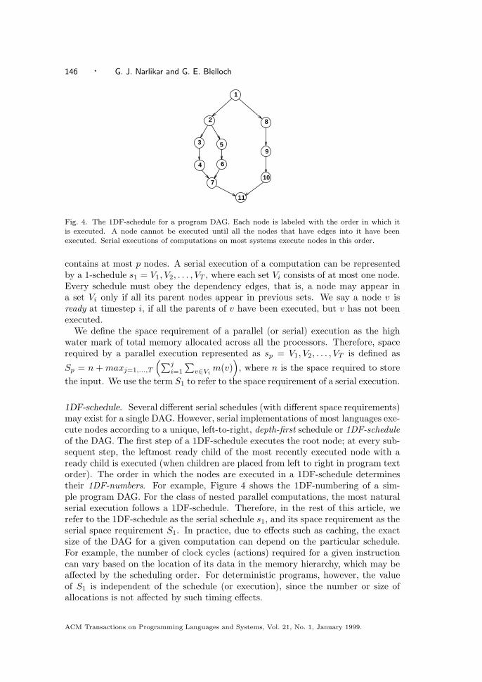
Fig. 4. The 1DF-schedule for a program DAG. Each node is labeled with the order in which itis executed. A node cannot be executed until all the nodes that have edges into it have beenexecuted. Serial executions of computations on most systems execute nodes in this order.
contains at most p nodes. A serial execution of a computation can be representedby a 1-schedule s1 = V1, V2, . . . , VT , where each set Vi consists of at most one node.Every schedule must obey the dependency edges, that is, a node may appear ina set Vi only if all its parent nodes appear in previous sets. We say a node v isready at timestep i, if all the parents of v have been executed, but v has not beenexecuted.
We define the space requirement of a parallel (or serial) execution as the highwater mark of total memory allocated across all the processors. Therefore, spacerequired by a parallel execution represented as sp = V1, V2, . . . , VT is defined as
Sp = n + maxj=1,...,T
(∑ji=1
∑v∈Vim(v)
), where n is the space required to store
the input. We use the term S1 to refer to the space requirement of a serial execution.
1DF-schedule. Several different serial schedules (with different space requirements)may exist for a single DAG. However, serial implementations of most languages exe-cute nodes according to a unique, left-to-right, depth-first schedule or 1DF-scheduleof the DAG. The first step of a 1DF-schedule executes the root node; at every sub-sequent step, the leftmost ready child of the most recently executed node with aready child is executed (when children are placed from left to right in program textorder). The order in which the nodes are executed in a 1DF-schedule determinestheir 1DF-numbers. For example, Figure 4 shows the 1DF-numbering of a sim-ple program DAG. For the class of nested parallel computations, the most naturalserial execution follows a 1DF-schedule. Therefore, in the rest of this article, werefer to the 1DF-schedule as the serial schedule s1, and its space requirement as theserial space requirement S1. In practice, due to effects such as caching, the exactsize of the DAG for a given computation can depend on the particular schedule.For example, the number of clock cycles (actions) required for a given instructioncan vary based on the location of its data in the memory hierarchy, which may beaffected by the scheduling order. For deterministic programs, however, the valueof S1 is independent of the schedule (or execution), since the number or size ofallocations is not affected by such timing effects.
ACM Transactions on Programming Languages and Systems, Vol. 21, No. 1, January 1999.
Space-Efficient Scheduling of Nested Parallelism · 147
Processors
Qout
Q in
R
decreasing threadpriorities
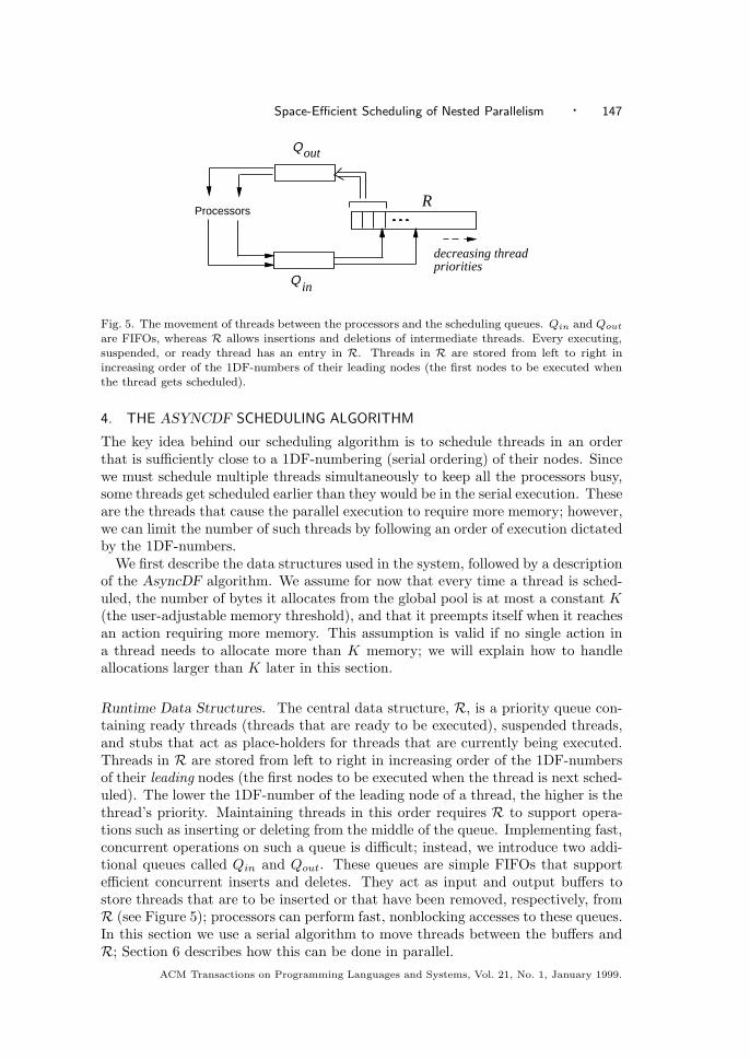
Fig. 5. The movement of threads between the processors and the scheduling queues. Qin and Qoutare FIFOs, whereas R allows insertions and deletions of intermediate threads. Every executing,suspended, or ready thread has an entry in R. Threads in R are stored from left to right inincreasing order of the 1DF-numbers of their leading nodes (the first nodes to be executed whenthe thread gets scheduled).
4. THE ASYNCDF SCHEDULING ALGORITHM
The key idea behind our scheduling algorithm is to schedule threads in an orderthat is sufficiently close to a 1DF-numbering (serial ordering) of their nodes. Sincewe must schedule multiple threads simultaneously to keep all the processors busy,some threads get scheduled earlier than they would be in the serial execution. Theseare the threads that cause the parallel execution to require more memory; however,we can limit the number of such threads by following an order of execution dictatedby the 1DF-numbers.
We first describe the data structures used in the system, followed by a descriptionof the AsyncDF algorithm. We assume for now that every time a thread is sched-uled, the number of bytes it allocates from the global pool is at most a constant K(the user-adjustable memory threshold), and that it preempts itself when it reachesan action requiring more memory. This assumption is valid if no single action ina thread needs to allocate more than K memory; we will explain how to handleallocations larger than K later in this section.
Runtime Data Structures. The central data structure, R, is a priority queue con-taining ready threads (threads that are ready to be executed), suspended threads,and stubs that act as place-holders for threads that are currently being executed.Threads in R are stored from left to right in increasing order of the 1DF-numbersof their leading nodes (the first nodes to be executed when the thread is next sched-uled). The lower the 1DF-number of the leading node of a thread, the higher is thethread’s priority. Maintaining threads in this order requires R to support opera-tions such as inserting or deleting from the middle of the queue. Implementing fast,concurrent operations on such a queue is difficult; instead, we introduce two addi-tional queues called Qin and Qout. These queues are simple FIFOs that supportefficient concurrent inserts and deletes. They act as input and output buffers tostore threads that are to be inserted or that have been removed, respectively, fromR (see Figure 5); processors can perform fast, nonblocking accesses to these queues.In this section we use a serial algorithm to move threads between the buffers andR; Section 6 describes how this can be done in parallel.
ACM Transactions on Programming Languages and Systems, Vol. 21, No. 1, January 1999.

148 · G. J. Narlikar and G. E. Blelloch
begin workerwhile (there exist threads in the system)τ := remove-thread(Qout);if (τ is a scheduling thread) then scheduler()else
execute the actions associated with τ ;if (τ terminates) or (τ suspends) or (τ preempts itself)then insert-thread(τ , Qin);
end worker
begin scheduleracquire scheduler-lock;
insert a scheduling thread into Qout;T := remove-all-threads(Qin);for each thread τ in T
insert τ into R in its original position;if τ has terminated
if τ is the last among its siblings to synchronize,reactivate τ ’s parent;
delete τ from R;select the leftmost p ready threads from R:
if there are less than p ready threads, select them all;fork child threads in place if needed;
insert these selected threads into Qout;release scheduler-lock;
end scheduler
Fig. 6. The AsyncDF scheduling algorithm. When the scheduler forks (creates) child threads, itinserts them into R in the immediate left of their parent thread. This maintains the invariantthat the threads in R are always in the order of increasing 1DF-numbers of their leading nodes.Therefore, at every scheduling step, the p ready threads whose leading nodes have the smallest1DF-numbers are moved to Qout. Child threads are forked only when they are to be added toQout, that is, when they are among the leftmost p ready threads in R.
Algorithm Description. The pseudocode for the AsyncDF scheduling algorithm isgiven in Figure 6. The processors normally act as workers, when they take threadsfrom Qout, execute them until they preempt themselves, suspend or terminate,and then return them to Qin. Every time a ready thread is picked from Qout andscheduled on a worker processor, it may allocate space from a global pool in its firstaction. The thread must preempt itself before any subsequent action that requiresmore space. A thread that performs a fork must suspend itself; it is reactivatedwhen the last of its forked child threads terminates. A child thread terminates uponreaching the synchronization point.
In addition to acting as workers, the processors take turns in acting as the sched-uler. For this purpose, we introduce special scheduling threads into the system.Whenever the thread taken from Qout by a processor turns out to be a schedulingthread, it assumes the role of the scheduling processor and executes the schedulerprocedure. We call each execution of the scheduler procedure a scheduling step.Only one processor can be executing a scheduling step at a time due to the sched-uler lock. The algorithm begins with a scheduling thread and the first (root) threadof the program on Qout.
A processor that executes a scheduling step starts by putting a new schedulingACM Transactions on Programming Languages and Systems, Vol. 21, No. 1, January 1999.

Space-Efficient Scheduling of Nested Parallelism · 149
thread on Qout. Next, it moves all the threads from Qin to R. Each thread has apointer to a stub that marks its original position relative to the other threads inR; itis inserted back in that position. All threads that were preempted due to a memoryallocation are returned to R in the ready state. The scheduler then compacts R byremoving threads that have terminated. These are child threads that have reachedtheir synchronization point and the root thread at the end of the entire computation.If a thread is the last among its siblings to reach its synchronization point, itssuspended parent thread is reactivated. If a thread performs a fork, its child threadsare inserted to its immediate left, and the forking thread suspends. The childthreads are placed inR in order of the 1DF-numbers of their leading nodes. Finally,the scheduler moves the leftmost p ready threads from R to Qout, leaving behindstubs to mark their positions in R. If R contains less than p ready threads, thescheduler moves them all to Qout. The scheduling thread then completes, and theprocessor resumes the task of a worker.
This scheduling algorithm ensures that the total number of threads in Qin andQout is at most 3p (see Lemma 5.1.4). Further, to limit the number of threads in R,we lazily create the child threads of a forking thread: a child thread is not explicitlycreated until it is to be moved to Qout, that is, when it is among the leftmost pthreads represented in R. Until then, the parent thread implicitly represents thechild thread. A single parent may represent several child threads. This optimizationensures that a thread does not have an entry in R until it has been scheduled atleast once before, or is in (or about to be inserted into) Qout. If a thread τ is readyto fork child threads, all its child threads will be forked (created) and scheduledbefore any other threads in R to the right of τ can be scheduled.
Handling Large Allocations of Space. We had assumed earlier in this section thatevery time a thread is scheduled, it allocates at most K bytes for its use from aglobal pool of memory, where K is the constant memory threshold. This does notallow any single action within a thread to allocate more than K bytes. We now showhow such allocations are handled, similar to the technique suggested in previouswork [Blelloch et al. 1995]. The key idea is to delay the big allocations, so thatif threads with lower 1DF-numbers become ready, they will be executed instead.Consider a thread with a node that allocates m units of space in the original DAG,and m > K. We transform the DAG by inserting a fork of m/K parallel threadsbefore the memory allocation (see Figure 7). These new child threads performa unit of work (a no-op), but do not allocate any space; they simply consist ofdummy nodes. However, we treat the dummy nodes as if they allocate space, andthe original thread is suspended at the fork. It is reactivated when all the dummythreads have been executed, and may now proceed with the allocation of m space.This transformation of the DAG increases its depth by at most a constant factor. IfSa is the total space allocated in the program (not counting the deallocations), thenumber of nodes in the transformed DAG is at most W+Sa/K. The transformationtakes place at runtime, and the on-line AsyncDF algorithm generates a schedule forthis transformed DAG. This ensures that the space requirement of the generatedschedule does not exceed our space bounds, as proved in Section 5.
We state the following lemma regarding the order of the nodes in R maintainedby the AsyncDF algorithm.
ACM Transactions on Programming Languages and Systems, Vol. 21, No. 1, January 1999.

150 · G. J. Narlikar and G. E. Blelloch
(a) (b)
. . .
threads
0
0 m K
0
m0 0
m
Fig. 7. A transformation of the DAG to handle a large allocation of space at a node withoutviolating the space bound. Each node is labeled with the amount of memory its action allocates.When a thread needs to allocate m space (m > K), we insert m/K parallel child threads beforethe allocation. K is the constant memory threshold. Each child thread consists of a dummy nodethat does not allocate any space. After these child threads complete execution, the original threadperforms the allocation and continues with its execution.
Lemma 4.1. The AsyncDF scheduling algorithm always maintains the threadsin R in an increasing order of the 1DF-numbers of their leading nodes.
Proof. This lemma can be proved by induction. When the execution begins,R contains just the root thread, and therefore it is ordered by the 1DF-numbers.Assume that at the start of some scheduling step, the threads in R are in increasingorder of the 1DF-numbers of their leading nodes. For a thread that forks, insertingits child threads before it in the order of their 1DF-numbers maintains the orderingby 1DF-numbers. A thread that preempts itself due to a memory allocation is re-turned to its original position in the ready state. Its new leading node has the same1DF-number as its previous leading node, relative to leading nodes of other threads.Deleting threads from R does not affect their ordering. Therefore the ordering ofthreads in R by 1DF-numbers is preserved after every operation performed by thescheduler.
Lemma 4.1 implies that when the scheduler moves the leftmost p threads from Rto Qout, their leading nodes are the nodes with the lowest 1DF-numbers. We willuse this fact to prove the space bounds of the schedule generated by our schedulingalgorithm.
5. THEORETICAL RESULTS
In this section, we prove that a parallel computation with depth D and work W ,which requires S1 space to execute on one processor, is executed by the AsyncDFscheduling algorithm on p processors using S1 +O(D · p) space (including schedulerspace). In Section 6 we describe the implementation of a parallelized scheduler andanalyze both the space and time bounds including scheduler overheads.
Recall that we defined a single action as the work done by a thread in onetimestep (clock cycle). Since the granularity of a clock-cycle is somewhat arbitrary,especially considering highly pipelined processors with multiple functional units,this would seem to make the exact value of the depth D somewhat arbitrary. Forasymptotic bounds this is not problematic, since the granularity will only makeACM Transactions on Programming Languages and Systems, Vol. 21, No. 1, January 1999.

Space-Efficient Scheduling of Nested Parallelism · 151
constant factor differences. In Appendix A, however, we modify the space boundto be independent of the granularity of actions, making it possible to bound thespace requirement within tighter constant factors.
Timing Assumptions. As explained in Section 3, the timesteps are synchronizedacross all the processors. At the start of each timestep, we assume that a workerprocessor is either busy executing a thread or is accessing the queues Qout or Qin.An idle processor always busy waits for threads to appear in Qout. We assumea constant-time, atomic fetch-and-add operation in our system. This allows allworker processors to access Qin and Qout in constant time [Narlikar 1999]. Thus,at any timestep, if Qout has n threads, and pi processors are idle, then min(n, pi)of the pi idle processors are guaranteed to succeed in picking a thread from Qoutwithin a constant number of timesteps. We do not need to limit the duration ofeach scheduling step to prove the space bound; we simply assume that it takes atleast one timestep to execute.
5.1 Space Bound
To prove the space bound, we partition the nodes of the computation DAG intoheavy and light nodes. Every time a ready thread is scheduled, we call the noderepresenting its first action (i.e., the thread’s leading node) a heavy node, and allother nodes light nodes. Thus, heavy nodes may allocate space, while light nodesallocate no space (but may deallocate space). The space requirement is analyzedby bounding the number of heavy nodes that execute out of order with respectto the 1DF-schedule. When a thread is moved from R to Qout by a schedulingprocessor, we will say its leading heavy node has been inserted into Qout. A heavynode may get executed several timesteps after it becomes ready and after it is putinto Qout. However, a light node is executed in the timestep it becomes ready,because a processor executes consecutive light nodes nonpreemptively.
Let sp = V1, . . . , VT be the parallel schedule of the DAG generated by theAsyncDF algorithm. Here Vi is the set of nodes that are executed at timestepi. Let s1 be the 1DF-schedule for the same DAG. A prefix of sp is the set
⋃ ji=1 Vi,
that is, the set of all nodes executed during the first j timesteps of sp, for any1 ≤ j ≤ T . Consider an arbitrary prefix, σp, of sp. Let σ1 be the largest prefix ofs1 containing only nodes in σp, that is, σ1 does not contain any nodes that are notpart of σp. Then σ1 is the corresponding serial prefix of σp. We call the nodes inσp − σ1 the premature nodes, because they have been executed out of order withrespect to s1. All other nodes in σp (i.e., all nodes in the set σ1) are called nonpre-mature. For example, Figure 8 shows a simple DAG with a parallel prefix σp forsome arbitrary p-schedule, and its corresponding serial prefix σ1.
The parallel execution has higher memory requirements because of the spaceallocated by the actions associated with the premature nodes. Hence we need tobound the space overhead of the premature nodes in σp. To get this bound, weneed to consider only the heavy premature nodes, since the light nodes do notallocate any space. We will assume for now that the actions corresponding to allheavy nodes allocate at most K space each, where K is the user-specified memorythreshold of the scheduler. Later we will relax this assumption to cover biggerallocations. We first prove the following bound on the number of heavy nodes that
ACM Transactions on Programming Languages and Systems, Vol. 21, No. 1, January 1999.
152 · G. J. Narlikar and G. E. Blelloch
a
b
c e
f
g
h
i
j
k
l
m
n
d
a
b
c e
f
g
h
i
j
k
l
m
n
d
1
p
O
O
(a) (b)
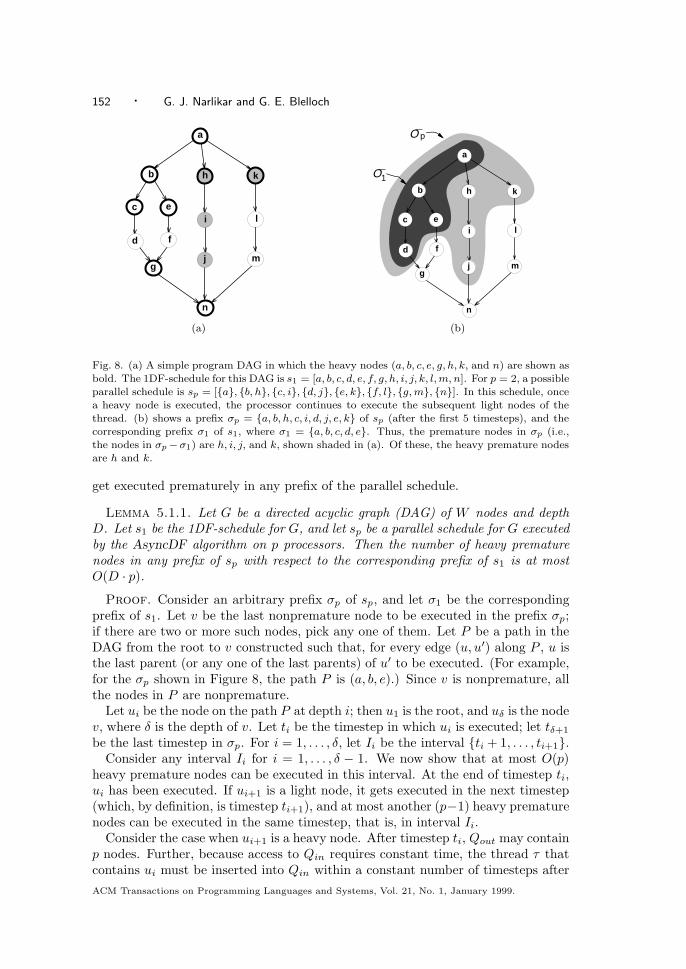
Fig. 8. (a) A simple program DAG in which the heavy nodes (a, b, c, e, g, h, k, and n) are shown asbold. The 1DF-schedule for this DAG is s1 = [a, b, c, d, e, f, g, h, i, j, k, l,m, n]. For p = 2, a possibleparallel schedule is sp = [{a}, {b, h}, {c, i}, {d, j}, {e, k}, {f, l}, {g,m}, {n}]. In this schedule, oncea heavy node is executed, the processor continues to execute the subsequent light nodes of thethread. (b) shows a prefix σp = {a, b, h, c, i, d, j, e, k} of sp (after the first 5 timesteps), and thecorresponding prefix σ1 of s1, where σ1 = {a, b, c, d, e}. Thus, the premature nodes in σp (i.e.,the nodes in σp−σ1) are h, i, j, and k, shown shaded in (a). Of these, the heavy premature nodesare h and k.
get executed prematurely in any prefix of the parallel schedule.
Lemma 5.1.1. Let G be a directed acyclic graph (DAG) of W nodes and depthD. Let s1 be the 1DF-schedule for G, and let sp be a parallel schedule for G executedby the AsyncDF algorithm on p processors. Then the number of heavy prematurenodes in any prefix of sp with respect to the corresponding prefix of s1 is at mostO(D · p).
Proof. Consider an arbitrary prefix σp of sp, and let σ1 be the correspondingprefix of s1. Let v be the last nonpremature node to be executed in the prefix σp;if there are two or more such nodes, pick any one of them. Let P be a path in theDAG from the root to v constructed such that, for every edge (u, u′) along P , u isthe last parent (or any one of the last parents) of u′ to be executed. (For example,for the σp shown in Figure 8, the path P is (a, b, e).) Since v is nonpremature, allthe nodes in P are nonpremature.
Let ui be the node on the path P at depth i; then u1 is the root, and uδ is the nodev, where δ is the depth of v. Let ti be the timestep in which ui is executed; let tδ+1
be the last timestep in σp. For i = 1, . . . , δ, let Ii be the interval {ti + 1, . . . , ti+1}.Consider any interval Ii for i = 1, . . . , δ − 1. We now show that at most O(p)
heavy premature nodes can be executed in this interval. At the end of timestep ti,ui has been executed. If ui+1 is a light node, it gets executed in the next timestep(which, by definition, is timestep ti+1), and at most another (p−1) heavy prematurenodes can be executed in the same timestep, that is, in interval Ii.
Consider the case when ui+1 is a heavy node. After timestep ti, Qout may containp nodes. Further, because access to Qin requires constant time, the thread τ thatcontains ui must be inserted into Qin within a constant number of timesteps afterACM Transactions on Programming Languages and Systems, Vol. 21, No. 1, January 1999.

Space-Efficient Scheduling of Nested Parallelism · 153
ti. During these timesteps, a constant number of scheduling steps may be executed,adding another O(p) threads into Qout. Thus, because Qout is a FIFO, a total ofO(p) heavy nodes may be picked from Qout and executed before ui+1; all of theseheavy nodes may be premature. However, once the thread τ is inserted into Qin, thenext scheduling step must find it in Qin; since ui is the last parent of ui+1 to execute,this scheduling step makes ui+1 available for scheduling. Thus, this scheduling stepor any subsequent scheduling step must put ui+1 on Qout before it puts any morepremature nodes, because ui+1 has a lower 1DF-number. When ui+1 is picked fromQout and executed by a worker processor, another p − 1 heavy premature nodesmay get executed by the remaining worker processors in the same timestep, which,by definition, is timestep ti+1. Thus, a total of O(p) heavy premature nodes maybe executed in interval Ii. Similarly, since v = uδ is the last nonpremature nodein σp, at most O(p) heavy premature nodes get executed in the last interval Iδ.Because δ ≤ D, σp contains a total of O(D · p) heavy premature nodes.
We have shown that any prefix of sp has at most O(D ·p) heavy premature nodes.Since we have assumed that the action associated with each heavy node allocatesat most K space, we can prove the following lemma.
Lemma 5.1.2. Let G be a program DAG with depth D, in which every heavy nodeallocates at most K space. If the serial execution of the DAG requires S1 space,then the AsyncDF scheduling algorithm results in an execution on p processors thatrequires at most S1 +O(K ·D · p)space.
Proof. Consider any parallel prefix σp of the parallel schedule generated byalgorithm AsyncDF; let σ1 be the corresponding serial prefix. The net memoryallocation of the nodes in σ1 is at most S1, because σ1 is a prefix of the serialschedule. Further, according to Lemma 5.1.1, the set σp − σ1 has O(D · p) heavynodes, each of which may allocate at most K space. Therefore, the net spaceallocated by all the nodes in σp is at most S1 +O(K ·D ·p). Since this bound holdsfor any arbitrary prefix of the parallel execution, the entire parallel execution alsouses at most S1 +O(K ·D · p) space.
Handling Allocations Bigger than the Memory Threshold K. We described how totransform the program DAG to handle allocations bigger than K bytes in Section 4.Consider any heavy premature node v that allocates m > K space. The m/Kdummy nodes inserted before it would have been executed before it. Being dummynodes, they do not actually allocate any space, but are entitled to allocate a totalof m space (K units each) according to our scheduling technique. Hence v canallocate these m units without exceeding the space bound in Lemma 5.1.2. Withthis transformation, a parallel computation withW work andD depth that allocatesa total of Sa units of memory results in a DAG with at most W +Sa/K nodes andO(D) depth. Therefore, using Lemma 5.1.2, we can state the following lemma.
Lemma 5.1.3. A computation of depth D and work W , which requires S1 spaceto execute on one processor, is executed on p processors by the AsyncDF algorithmusing S1 +O(K ·D · p) space.
Finally, we bound the space required by the scheduler to store the three queues.
ACM Transactions on Programming Languages and Systems, Vol. 21, No. 1, January 1999.

154 · G. J. Narlikar and G. E. Blelloch
Lemma 5.1.4. The space required by the scheduler is O(D · p).
Proof. When a processor starts executing a scheduling step, it first empties Qin.At this time, there can be at most p− 1 threads running on the other processors,and Qout can have another p threads in it. The scheduler adds at most another pthreads (plus one scheduling thread) to Qout, and no more threads are added toQoutuntil the next scheduling step. Since all the threads executing on the processorscan end up in Qin, Qin and Qout can have a total of at most 3p threads at anytime. Finally, we bound the number of threads in R. We will call a thread that hasbeen created but not yet deleted from the system a live thread; R has one entryfor each live thread. At any stage during the execution, the number of live threadsis at most the number of premature nodes executed, plus the maximum numberof threads in Qout (which is 2p+ 1), plus the maximum number of live threads inthe 1DF-schedule. Any step of the 1DF-schedule can have at most D live threads,because it executes threads in a depth-first manner. Since the number of prematurenodes is at most O(D · p), R has at most O(D · p+D+ 2p+ 1) = O(D · p) threads.Because each thread requires a small, constant c units of memory to store its state,4
the total space required by the three scheduling queues is O(c ·D · p) = O(D · p).
Using Lemmas 5.1.3 and 5.1.4, we can now state the following bound on the totalspace requirement of the parallel computation.
Theorem 5.1.5. A computation of depth D and work W , which requires S1
space to execute on one processor, is executed on p processors by the AsyncDFalgorithm using S1 +O(K ·D · p) space (including scheduler space).
In practice, K is set to a small, constant amount of memory throughout the exe-cution of the program (see Section 7), reducing the space bound to S1 +O(D · p).
5.2 Time Bound
Finally, we bound the time required to execute the parallel schedule generated bythe scheduling algorithm for a special case; Section 6 analyzes the time bound inthe general case. In this special case, we assume that the worker processors neverhave to wait for the scheduler to add ready threads to Qout. Thus, when there arer ready threads in the system, and n processors are idle, Qout has at least min(r, n)ready threads. Then min(r, n) of the idle processors are guaranteed to pick readythreads from Qout within a constant number of timesteps. We can show that thetime required for such an execution is within a constant factor of the time requiredto execute a greedy schedule. A greedy schedule is one in which at every timestep, ifn nodes are ready, min(n, p) of them get executed. Previous results have shown thatgreedy schedules for DAGs with W nodes and D depth require at most W/p + Dtimesteps to execute [Blumofe and Leiserson 1993]. Our transformed DAG hasW + Sa/K nodes and O(D) depth. Therefore, we can show that our schedulerrequires O(W/p + Sa/pK + D) timesteps to execute on p processors. When the
4Recall that a thread allocates stack and heap data from the global pool of memory that is assignedto it every time it is scheduled; the data are hence accounted for in the space bound proved inLemma 5.1.3 Therefore, the thread’s state here refers simply to its register contents.
ACM Transactions on Programming Languages and Systems, Vol. 21, No. 1, January 1999.
Space-Efficient Scheduling of Nested Parallelism · 155
allocated space Sa is O(W ), the number of timesteps required is O(W/p+D). Fora more in-depth analysis of the running time that includes the cost of a parallelizedscheduler in the general case, see Section 6.
6. A PARALLELIZED SCHEDULER
The time bound in Section 5 was proved for the special case when the schedulerprocedure never becomes a bottleneck in making ready threads available to theworker processors. However, recall that the scheduler in the AsyncDF algorithmis a serial scheduler, that is, only one processor can be executing the schedulerprocedure at a given time. Further, the time required for this procedure to executemay increase with the number of processors, causing idle worker processors towait longer for ready threads to appear Qout. Thus, the scheduler may indeedbecome a bottleneck on a large number of processors. Therefore, the schedulermust be parallelized to scale with the number of processors. In this section, wedescribe a parallel implementation of the scheduler and analyze its space and timecosts. We prove that a computation with W work and D depth can be executed inO(W/p+Sa/p+D · log p) time and S1 +O(D ·p · log p) space on p processors; thesebounds include the overheads of the parallelized scheduler. The additional log pterm in the time bound arises due to the parallel prefix operations executed by thescheduler. The log p term in the space bound is due to the additional number ofready threads created to keep worker processors busy while the scheduler executes.
We give only a theoretical description of a parallelized scheduler in this article;the experimental results presented in Section 7 have been obtained using the serialscheduler from Figure 6. As our results on up to 16 processors demonstrate, theserial scheduler provides good performance on this moderate number of processors.
6.1 Parallel Implementation of a Lazy Scheduler
Instead of using scheduler threads to periodically (and serially) execute the sched-uler procedure as shown in Figure 6, we devote a constant fraction αp of the pro-cessors (0 < α < 1) to it. The remaining (1 − α)p processors always execute asworkers. To amortize the cost of the scheduler, we place a larger number of threads(up to p log p instead of p) into Qout. As in Section 5, we assume that a thread canbe inserted or removed from Qin or Qout by any processor in constant time. Thedata structure R is implemented as an array of threads, stored in decreasing orderof priorities from left to right.
As described in Section 4, threads are forked lazily; when a thread reaches afork, it is simply marked as a seed thread. At a later time, when its child threadsare to be scheduled, they are placed to the immediate left of the seed in order oftheir 1DF-numbers. Similarly, we perform all deletions lazily: every thread thatterminates is simply marked inR as a dead thread, to be deleted in some subsequenttimestep.
The synchronization (join) between child threads of a forking thread is imple-mented using a fetch-and-decrement operation on a synchronization counter asso-ciated with the fork. Each child that reaches the synchronization point decrementsthe counter by one and checks its value. If the counter has nonzero value, it simplymark itself as dead. The last child thread to reach the synchronization point (theone that decrements the counter to zero) marks itself as ready in R, and subse-
ACM Transactions on Programming Languages and Systems, Vol. 21, No. 1, January 1999.

156 · G. J. Narlikar and G. E. Blelloch
quently continues as the parent. Thus, when all the child threads have been created,the seed that originally represented the parent thread can be deleted.
We will refer to all the threads that have an entry in R but are not dead aslive threads. For every ready (or seed) thread τ that has an entry in R, we usea nonnegative integer c(τ) to describe its state: c(τ) equals the number of readythreads τ represents. Then for every seed τ , c(τ) is the number of child threadsstill to be created from it. For every other ready thread in R, c(τ) = 1, because itrepresents itself.
The scheduler procedure from Figure 6 can now be replaced by a while loop thatruns until the entire computation has been executed. Each iteration of this loop,which we call a scheduling iteration, is executed in parallel by only the αp schedulerprocessors. Therefore, it need not be protected by a scheduler lock as in Figure 6.Let r be the total number of ready threads represented in R after threads from Qinare moved to R at the beginning of the iteration. Let qo = min(r, p log p− |Qout|)be the number of threads the scheduling iteration will move to Qout. The schedulingiteration of a lazy scheduler is defined as follows.
(1) Collect all the threads from Qin and move them to R, that is, update theirstates in R.
(2) Delete all the dead threads up to the leftmost (qo + 1) ready or seed threads.
(3) Perform a prefix-sums computation on the c(τ) values of the leftmost qo readyor seed threads to find the set C of the leftmost qo ready threads representedby these threads. For every thread in C that is represented implicitly by a seed,create an entry for the thread in R, marking it as a ready thread. Mark theseeds for which all child threads have been created as dead.
(4) Move the threads in the set C from R to Qout, leaving stubs in R to mark theirpositions.
Consider a thread τ that is the last child thread to reach the synchronization pointin a fork, but was not the rightmost thread among its siblings. Some of τ ’s siblings,which have terminated, may be represented as dead threads to its right. Since τnow represents the parent thread after the synchronization point, it has a higher1DF-number than these dead siblings to its immediate right. Thus, due to lazydeletions, dead threads may be out of order in R. However, the scheduler deletesall dead threads up to the first (qo + 1) ready or seed threads, that is, all deadthreads to the immediate right of any ready thread (or seed representing a readythread) before it is scheduled. Therefore, no descendents of a thread may be createduntil all dead threads out of order with respect to the thread are deleted. Thus, athread may be out of order with only the dead threads to its immediate right.
We say a thread is active when it is either in Qout or Qin, or when it is being exe-cuted on a processor. Once a scheduling iteration empties Qin, at most p log p+(1−α)p threads are active. The iteration creates at most another p log p active threadsbefore it ends, and no more threads are made active until the next scheduling step.Therefore at most 2p log p + (1 − α)p threads can be active at any timestep, andeach has one entry in R. We now prove the following bound on the time requiredto execute a scheduling iteration.
ACM Transactions on Programming Languages and Systems, Vol. 21, No. 1, January 1999.

Space-Efficient Scheduling of Nested Parallelism · 157
Lemma 6.1.1. For any 0 < α < 1, a scheduling iteration that deletes n deadthreads runs in O( n
αp + log pα ) time on αp processors.
Proof. Let qo ≤ p log p be the number of threads the scheduling iterationmust move to Qout. At the beginning of the scheduling iteration, Qin containsat most 2p log p + (1 − α)p threads. Since each of these threads has a pointer toits stub in R, αp processors can move the threads to R in O( log p
α ) time. Let τbe the (qo + 1)th ready or seed thread in R (starting from the left end). Thescheduler needs to delete all dead threads to the left of τ . In the worst case, allthe stubs are also to the left of τ in R. However, the number of stubs in R is atmost 2p log p + (1 − α)p. Because there are n dead threads to the left of τ , theycan be deleted from n+ 2p log p+ (1−α)p threads in O( n
αp + log pα ) timesteps on αp
processors. After the deletions, the leftmost qo ≤ p log p ready threads are amongthe first 3p log p + (1 − α)p threads in R; therefore the prefix-sums computationwill require O( log p
α ) time. Finally, qo new child threads can be created and addedin order to the left end of R in O( log p
α ) time. Note that all deletions and additionsare at the left end of R, which are simple operations in an array.5 Thus, the entirescheduling iteration runs in O( n
αp + log pα ) time.
6.2 Space and Time Bounds Using the Parallelized Scheduler
We now state the space and time bounds of a parallel computation, includingscheduling overheads. The bounds assume that a constant fraction α of the pprocessors (for any 0 < α < 1) are dedicated to the task of scheduling. Thedetailed proofs are given in Appendix B.
Theorem 6.2.1. Let S1 be the space required by a 1DF-schedule for a compu-tation with work W and depth D, and let Sa be the total space allocated in thecomputation. The parallelized scheduler with a memory threshold of K units, gen-erates a schedule on p processors that requires S1 + O(K · D · p · log p) space andO(W/p+ Sa/pK +D · log p) time to execute.
These time and space bounds include scheduling overheads. The time bound isderived by counting the total number of timesteps during which the worker proces-sors may be either idle or busy executing actions. The space bound is proved usingan approach similar to that used in Section 5. When the total space allocatedSa = O(W ), the time bound reduces to O(W/p + D · log p). As with the serialscheduler, when the memory threshold K is set to a constant, the asymptotic spacebound reduces to S1 + O(D · p · log p).
7. EXPERIMENTAL RESULTS
We have built a runtime system that uses the AsyncDF algorithm to scheduleparallel threads, and have run several experiments to analyze both the time and thememory required by parallel computations. In this section we briefly describe theimplementation of the system and the benchmarks used to evaluate its performance,followed by the experimental results.
5The additions and deletions must skip over the stubs to the left of τ , which can add at mosta log p
αdelay.
ACM Transactions on Programming Languages and Systems, Vol. 21, No. 1, January 1999.

158 · G. J. Narlikar and G. E. Blelloch
7.1 Implementation
The runtime system has been implemented on a 16-processor SGI Power Challenge,which has a shared-memory architecture with processors and memory connected viaa fast shared-bus interconnect. We implemented the serial version of the schedulerpresented in Figure 6, because the number of processors on this architecture isnot very large. The set of ready threads R is implemented as a simple, singly-linked list. Qin and Qout, which are accessed by the scheduler and the workers,are required to support concurrent enqueue and dequeue operations. They areimplemented using variants of previous lock-free algorithms based on atomic fetch-and-Φ primitives [Mellor-Crummey 1987].
The parallel programs executed using this system have been explicitly hand-coded in the continuation-passing style, similar to the code generated by the Cilkpreprocessor6 [Blumofe et al. 1995]. Each continuation points to a C functionrepresenting the next computation of a thread, and a structure containing all itsarguments. These continuations are created dynamically and moved between thequeues. A worker processor takes a continuation off Qout, and simply applies thefunction pointed to by the continuation, to its arguments. The high-level programis broken into such functions at points where it executes a parallel fork, a recursivecall, or a memory allocation.
For nested parallel loops, we group iterations of the innermost loop into equallysized chunks, provided it does not contain calls to any recursive functions.7 Schedul-ing a chunk at a time improves performance by reducing scheduling overheads andproviding good locality, especially for fine-grained iterations.
Instead of preallocating a pool of memory for a thread every time it is scheduled,we use a memory counter to keep track of a thread’s net memory allocation. Thememory counter is initialized to the value of the memory threshold K when thethread is scheduled. The counter is appropriately decremented (incremented) whenthe thread allocates (deallocates) space. When the thread reaches a memory allo-cation that requires more memory than the current value of the counter, the threadis preempted, and the counter is reset to K units. Instead of explicitly creatingdummy threads to delay an allocation of m bytes (m > K) in a thread, the threadis inserted into R with a delay counter initialized to the value m/K. The delaycounter is appropriately decremented by the scheduling thread; each decrement by1 represents the creation and scheduling of one dummy thread. The original threadis ready to execute once the value of the delay counter is reduced to zero. Unlessstated otherwise, all the experiments described in this section were performed usingK = 1000 bytes.
7.2 Benchmark Programs
We implemented five parallel programs on our runtime system. We briefly describethe implementation of these programs, along with the problem sizes we used in ourexperiments.
6We expect a preprocessor-generated version on our system to have similar efficiency as thestraightforward hand-coded version.7It should be possible to automate such coarsening with compiler support.
ACM Transactions on Programming Languages and Systems, Vol. 21, No. 1, January 1999.

Space-Efficient Scheduling of Nested Parallelism · 159
(1) Blocked recursive matrix multiply (Rec MM). This program multiplies twodense n × n matrices using a simple recursive divide-and-conquer method, andperforms O(n3) work. The recursion stops when the blocks are down to the size of64× 64, after which the standard row-column matrix multiply is executed serially.This algorithm significantly outperforms the row-column matrix multiply for largematrices (e.g., by a factor of over 4 for 1024 × 1024 matrices) because its use ofblocks results in better cache locality. At each step, the eight recursive calls aremade in parallel. Each recursive call needs to allocate temporary storage, whichis deallocated before returning from the call. The results reported are for themultiplication of two 1024× 1024 matrices of double-precision floats.
(2) Strassen’s matrix multiply (Str MM). The DAG for this algorithm is verysimilar to that of the blocked recursive matrix multiply, but performs only O(n2.807)work and makes seven recursive calls at each step [Strassen 1969]. Once again, asimple serial matrix multiply is used at the leaves of the recursion tree. The sizesof matrices multiplied were the same as for the previous program.
(3) Fast multipole method (FMM). This is an n-body algorithm that calculatesthe forces between n bodies using O(n) work [Greengard 1987]. We have imple-mented the most time-consuming phases of the algorithm, which are a bottom-uptraversal of the octree followed by a top-down traversal. In the top-down traversal,for each level of the octree, the forces on the cells in that level due to their neigh-boring cells are calculated in parallel. For each cell, the forces over all its neighborsare also calculated in parallel, for which temporary storage needs to be allocated.This storage is freed when the forces over the neighbors have been added to getthe resulting force on that cell. With two levels of parallelism, the structure of thiscode looks very similar to the pseudocode described in Section 1. We executed theFMM on a uniform octree with 4 levels (83 leaves), using 5 multipole terms forforce calculation.
(4) Sparse matrix-vector multiplication (Sparse MV). This multiplies an m× nsparse matrix with an n × 1 dense vector. The dot product of each row of thematrix with the vector is calculated to get the corresponding element of the resultingvector. There are two levels of parallelism: over each row of the matrix and over theelements of each row multiplied with the corresponding elements of the vector tocalculate the dot product. For our experiments, we usedm = 20 and n = 1, 500, 000,and 30% of the elements were nonzeroes. (Using a large value of n provides sufficientparallelism within a row, but using large values of m leads to a very large size ofthe input matrix, making the amount of dynamic memory allocated in the programnegligible in comparison.)
(5) ID3. The ID3 algorithm [Quinlan 1986] builds a decision tree from a setof training examples in a top-down manner, using a recursive divide-and-conquerstrategy. At the root node, the attribute that best classifies the training data ispicked, and recursive calls are made to build subtrees, with each subtree using onlythe training examples with a particular value of that attribute. Each recursive callis made in parallel, and the computation of picking the best attribute at a node,which involves counting the number of examples in each class for different valuesfor each attribute, is also parallelized. Temporary space is allocated to store thesubset of training examples used to build each subtree and is freed once the subtree
ACM Transactions on Programming Languages and Systems, Vol. 21, No. 1, January 1999.
160 · G. J. Narlikar and G. E. Blelloch
0
2
4
6
8
10
12
14
1 4 8 12 16
Spe
edup
# Processors
Speedup curves
FMMFMM (Cilk)
Rec MMRec MM (Cilk)
Str MMStr MM (Cilk)
ID3ID3 (Cilk)
Sparse MVSparse MV (Cilk)
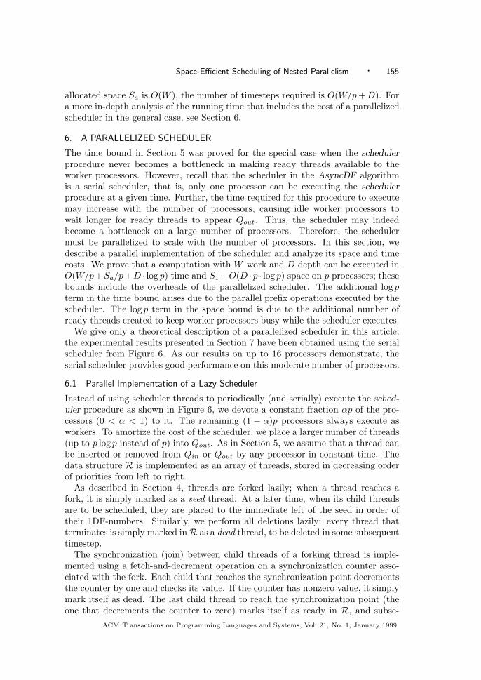
Fig. 9. The speedups achieved on up to 16 R10000 processors of a Power Challenge machine,using a value of K=1000 bytes. The speedup on p processors is the time taken for the serial Cversion of the program divided by the time for our runtime system to run it on p processors. Foreach application, the solid line represents the speedup using our system, while the dashed linerepresents the speedup using the Cilk system. All programs were compiled using gcc -O2 -mips2.
is built. We built a tree from 4 million test examples, each with 4 multivaluedattributes.
7.3 Time Performance
Figure 9 shows the speedups for the above programs for up to 16 processors. Thespeedup for each program is with respect to its efficient serial C version, whichdoes not use our runtime system. Since the serial C program runs faster thanour runtime system on a single processor, the speedup shown for one processoris less than 1. However, for all the programs, it is close to 1, implying that theoverheads in our system are low. The timings on our system include the delayintroduced before large allocations, in the form of m/K dummy nodes (K = 1000bytes) for an allocation of m bytes. Figure 9 also shows the speedups for the sameprograms running on an existing space-efficient system, Cilk [Blumofe et al. 1995],version 5.0. To make a fair comparison, we have chunked innermost iterations ofthe Cilk programs in the same manner as we did for our programs. The timingsshow that the performance on our system is comparable with that on Cilk. Thememory-intensive programs such as sparse matrix-vector multiply do not scale wellon either system beyond 12 processors; their performance is probably affected bybus contention as the number of processors increases.
Figure 10 shows the breakdown of the running time for one of the programs,blocked recursive matrix multiplication. The results show that the percentage ofACM Transactions on Programming Languages and Systems, Vol. 21, No. 1, January 1999.
Space-Efficient Scheduling of Nested Parallelism · 161
1 3 5 7 9 11 13 15
Number of processors (p)
0
10
20
30
40p
x ti
me
(sec
) Idle time
Queue access
Scheduling
Work overhead
Serial work
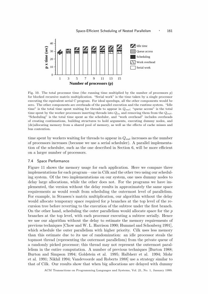
Fig. 10. The total processor time (the running time multiplied by the number of processors p)for blocked recursive matrix multiplication. “Serial work” is the time taken by a single processorexecuting the equivalent serial C program. For ideal speedups, all the other components would bezero. The other components are overheads of the parallel execution and the runtime system. “Idletime” is the total time spent waiting for threads to appear in Qout; “queue access” is the totaltime spent by the worker processors inserting threads into Qin and removing them from the Qout.“Scheduling” is the total time spent as the scheduler, and “work overhead” includes overheadsof creating continuations, building structures to hold arguments, executing dummy nodes, and(de)allocating memory from a shared pool of memory, as well as the effects of cache misses andbus contention.
time spent by workers waiting for threads to appear in Qout increases as the numberof processors increases (because we use a serial scheduler). A parallel implementa-tion of the scheduler, such as the one described in Section 6, will be more efficienton a larger number of processors.
7.4 Space Performance
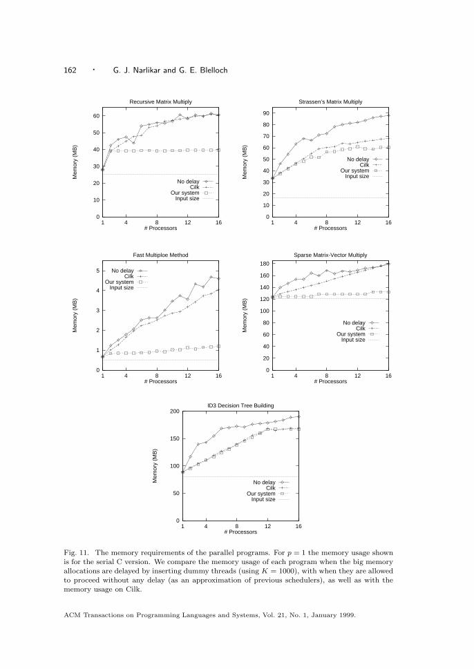
Figure 11 shows the memory usage for each application. Here we compare threeimplementations for each program—one in Cilk and the other two using our schedul-ing system. Of the two implementations on our system, one uses dummy nodes todelay large allocations, while the other does not. For the programs we have im-plemented, the version without the delay results in approximately the same spacerequirements as would result from scheduling the outermost level of parallelism.For example, in Strassen’s matrix multiplication, our algorithm without the delaywould allocate temporary space required for p branches at the top level of the re-cursion tree before reverting to the execution of the subtree under the first branch.On the other hand, scheduling the outer parallelism would allocate space for the pbranches at the top level, with each processor executing a subtree serially. Hencewe use our algorithm without the delay to estimate the memory requirements ofprevious techniques [Chow and W. L. Harrison 1990; Hummel and Schonberg 1991],which schedule the outer parallelism with higher priority. Cilk uses less memorythan this estimate due to its use of randomization: an idle processor steals thetopmost thread (representing the outermost parallelism) from the private queue ofa randomly picked processor; this thread may not represent the outermost paral-lelism in the entire computation. A number of previous techniques [Burton 1988;Burton and Simpson 1994; Goldstein et al. 1995; Halbherr et al. 1994; Mohret al. 1991; Nikhil 1994; Vandevoorde and Roberts 1988] use a strategy similar tothat of Cilk. Our results show that when big allocations are delayed with dummy
ACM Transactions on Programming Languages and Systems, Vol. 21, No. 1, January 1999.
162 · G. J. Narlikar and G. E. Blelloch
0
10
20
30
40
50
60
1 4 8 12 16
Mem
ory
(MB
)
# Processors
Recursive Matrix Multiply
No delayCilk
Our systemInput size
0
10
20
30
40
50
60
70
80
90
1 4 8 12 16
Mem
ory
(MB
)
# Processors
Strassen’s Matrix Multiply
No delayCilk
Our systemInput size
0
1
2
3
4
5
1 4 8 12 16
Mem
ory
(MB
)
# Processors
Fast Multiploe Method
No delayCilk
Our systemInput size
0
20
40
60
80
100
120
140
160
180
1 4 8 12 16
Mem
ory
(MB
)
# Processors
Sparse Matrix-Vector Multiply
No delayCilk
Our systemInput size
0
50
100
150
200
1 4 8 12 16
Mem
ory
(MB
)
# Processors
ID3 Decision Tree Building
No delayCilk
Our systemInput size
Fig. 11. The memory requirements of the parallel programs. For p = 1 the memory usage shownis for the serial C version. We compare the memory usage of each program when the big memoryallocations are delayed by inserting dummy threads (using K = 1000), with when they are allowedto proceed without any delay (as an approximation of previous schedulers), as well as with thememory usage on Cilk.
ACM Transactions on Programming Languages and Systems, Vol. 21, No. 1, January 1999.
Space-Efficient Scheduling of Nested Parallelism · 163
nodes, our algorithm results in a significantly lower memory usage, particularly asthe number of processors increases. A notable exception is the ID3 benchmark, forwhich our scheduler results in a similar space requirement as that of Cilk. Thisis because the value of K (1000 bytes) is too large to sufficiently delay the largeallocations of space until higher-priority threads become ready. Note that we havenot compared our scheduler to naive scheduling techniques, such as breadth-firstschedules resulting from the use of FIFO queues, which have much higher memoryrequirements.
Space-Time Trade-off. The number of dummy nodes introduced before a largeallocation and the frequency of thread preemptions depend on the value of thememory threshold K. Adjusting the value of K provides a trade-off between thememory usage and running time of a parallel computation. For example, Figure 1shows how the running time and memory usage for blocked recursive matrix mul-tiplication are affected by K. For very small K, many dummy nodes are inserted,and threads are preempted often; this results in a high running time. However, theexecution order (and therefore the space requirement) of the parallel schedule isclose to that of the serial schedule, leading to a low memory requirement. For verylarge K, very few dummy nodes are inserted, and threads are allowed to executelonger without being preempted; this leads to a high memory requirement and lowrunning time. For all the programs we implemented, the trade-off curves lookedsimilar; however, they may vary for other parallel programs. A default value ofK = 1000 bytes resulted in a good balance between space and time performancefor all our programs, although in practice it might be useful to allow users to tunethe parameter for their needs.
8. SUMMARY AND DISCUSSION
We have presented an asynchronous scheduling algorithm, AsyncDF, for languagesthat support nested parallelism, and have shown that it is space efficient and timeefficient in both theory and practice. The space bound presented in this article issignificantly lower than space bounds on existing space-efficient systems for pro-grams with a sufficient amount of parallelism (D � S1). Most parallel programs,including all programs in NC [Cook 1985], fall in this category. This article ana-lyzes the AsyncDF algorithm with both a serial and a parallel scheduler. We havebuilt a low-overhead runtime system that schedules parallel threads using the al-gorithm. The results demonstrate that our approach is more effective in reducingspace usage than previous scheduling techniques, and at the same time yields goodparallel performance. A more detailed specification of the theoretical frameworkon which the scheduling algorithm is based can be found elsewhere [Narlikar andBlelloch 1996].
We have added our scheduling technique to a native, lightweight implementationof POSIX standard threads [IEEE 1985] or Pthreads on Solaris [Powell et al. 1991].The results indicate that the new scheduler, unlike the existing FIFO scheduler, al-lows irregular and dynamic parallel programs written with a very large number ofPthreads to execute efficiently [Narlikar and Blelloch 1998]. We are currently work-ing on methods to further improve the scheduling algorithm, particularly to providebetter support for fine-grained threads. At present, fine-grained iterations of inner-
ACM Transactions on Programming Languages and Systems, Vol. 21, No. 1, January 1999.

164 · G. J. Narlikar and G. E. Blelloch
most loops are statically grouped into fixed-size chunks. A dynamic, decreasing-sizechunking scheme [Hummel et al. 1992; Kuck 1987; Tzen and Ni 1993] can be usedinstead. We are working on an algorithm to automatically coarsen the computa-tions at runtime by allowing the execution order to differ to a limited extent fromthe 1DF-numbers, and by using ordered, per-processor queues. Preliminary resultsindicate that this algorithm also results in reduced scheduling contention, becausethe processors access separate queues for a majority of the time.
APPENDIX
A. TIGHTER BOUND ON THE SPACE REQUIREMENT
In Section 5 we showed that algorithm AsyncDF executes a parallel computationwith depth D and serial space requirement S1 on p processors using S1 +O(p ·D)space. In particular, when actions that allocate space are represented by heavynodes, and each heavy node allocates at most K space (the value of the memorythreshold), we showed that any prefix of the parallel computation has O(p · D)heavy premature nodes. Here D is the maximum number of actions along any pathin the program DAG. Therefore, the value of D and the number of premature nodes(and hence the space bound) depends on the definition of an action; recall that anaction is a “unit” of work that may allocate or deallocate space, and requires atimestep to be executed. An action may be as small as a fraction of a machineinstruction, or as large as several machine instructions, depending on the definitionof a timestep. In this section, we give a more precise space bound by specifyingthe bound in terms of a ratio of the depth D, and the number of actions betweenconsecutive heavy nodes. Being a ratio of two values specified in terms of actions,it is no longer dependent on the granularity of an action.
Recall that heavy nodes may allocate K space and use it for subsequent actions,until the thread runs out of space and needs to perform another allocation. Thus,threads typically have heavy nodes followed by a large number of light nodes, andthe number of allocations (heavy nodes) along any path may be much smaller thanthe depth of the computation. We define the granularity g of the computation to bethe minimum number of actions (nodes) between two consecutive heavy nodes onany path in the program DAG, that is, the minimum number of actions executednonpreemptively by a thread every time it is scheduled. Note that the granularityof a computation depends on the value of the memory threshold K. In this section,we prove that the number of heavy premature nodes is O(p · D/g), and thereforethe parallel space requirement is S1 +O(p ·D/g).
Lemma A.1. Let G be a DAG with W nodes, depth D, and granularity g, inwhich every node allocates at most K space. Let s1 be the 1DF-schedule for G, andsp the parallel schedule for G executed by the AsyncDF algorithm on p processors.Then the number of heavy premature nodes in any prefix of sp with respect to thecorresponding prefix of s1 is O(p ·D/g).
Proof. The proof is similar to the proof for Lemma 5.1.1. Consider an arbitraryprefix σp of sp, and let σ1 be the corresponding prefix of s1. As with Lemma 5.1.1,we pick a path P from the root to the last nonpremature node v to be executedin σp, such that for every edge (u, u′) along the path, u is the last parent of u′ toACM Transactions on Programming Languages and Systems, Vol. 21, No. 1, January 1999.

Space-Efficient Scheduling of Nested Parallelism · 165
be executed. Let ui be the ith heavy node along P ; let δ be the number of heavynodes on P . Let ti be the timestep in which ui gets executed; let tδ+1 be the lasttimestep in σp. For i = 1, . . . , δ, let Ii be the interval {ti + 1, . . . , ti+1}.
Consider any Interval Ii, for i = 1, . . . , δ − 1. Let li be the number of nodesbetween ui and ui+1. Since all these nodes are light nodes, they get executedat timesteps ti + 1, . . . , ti + li. During these timesteps, the other p − 1 workerprocessors may execute heavy nodes; however, for each heavy node, they mustexecute at least (g − 1) light nodes. Therefore, each of these worker processorsmay execute at most dli/ge heavy premature nodes during the first li timesteps ofinterval Ii. At the end of timestep ti + li, there may be at most p nodes in Qout.Before the thread τ containing ui is inserted into Qin, at most another O(p) heavypremature nodes may be added to Qout. Further, (p − 1) heavy premature nodesmay execute along with ui+1. Hence O(p) < c · p heavy premature nodes (for someconstant c) may be executed before or with ui+1 after timestep ti + li. Thus, atotal of ((p− 1) · dli/ge+ c · p) heavy premature nodes get executed in the intervalIi. Similarly, we can bound the number of heavy premature nodes executed in thelast interval Iδ to ((p− 1) · dlδ/ge+ c · p).
Because there are δ ≤ D/g such intervals, and since∑δi=1 li ≤ D, the total
number of heavy premature nodes executed over all the δ intervals is at most
δ∑i=1
((p− 1) ·
⌈lig
⌉+ c · p
)≤
δ∑i=1
(p · (li/g + 1) + c · p)
≤ (c+ 1)p ·D/g + p/g ·δ∑i=1
li
= O(p ·D/g).
Similarly, we can prove that the scheduling queues require O(p · D/g) space;therefore, the computation requires a total of S1 +O(p ·D/g) space to execute onp processors.
Now consider a computation in which individual nodes allocate greater than Kspace. Let g1 be the original granularity of the DAG (by simply treating the nodesthat perform large allocations as heavy nodes). Now the granularity of this DAGmay change when we add dummy nodes before large allocations. Let g2 be thenumber of actions associated with the creation and execution of each of the dummythreads that we add to the DAG. Then the granularity of the transformed DAG isg = min(g1, g2). The space bound using the parallelized scheduler can be similarlymodified to S1 +O(D · p · log p/g).
Besides making the space bound independent of the definition of an action, thismodified bound is significantly lower than the original bound for programs with highgranularity g, that is, programs that perform a large number of actions betweenallocations, forks, or synchronizations.
ACM Transactions on Programming Languages and Systems, Vol. 21, No. 1, January 1999.
166 · G. J. Narlikar and G. E. Blelloch
B. PROOFS FOR THE SPACE AND TIME BOUNDS USING THE PARALLELIZEDSCHEDULER
In this section, we prove the space and time bounds for a parallel computationexecuted using the parallelized scheduler, as stated in Section 6 (Theorem 6.2.1).These bounds include the space and time overheads of the scheduler. We first definea class of DAGs that are more general than the DAGs used to represent parallelcomputations so far. This class of DAGs will be used to represent the computationthat is executed by using the parallelized scheduler.
Latency-Weighted DAGs. We extend the definition of a program DAG by allowingnonnegative weights on the edges; we call this new DAG a latency-weighted DAG.Let G = (V,E) be a latency-weighted DAG representing a parallel computation.Each edge (u, v) ∈ E has a nonnegative weight l(u, v) which represents the latencybetween the actions of the nodes u and v. The latency-weighted length of a pathin G is the sum of the total number of nodes in the path plus the sum of thelatencies on the edges along the path. We define latency-weighted depth Dl of Gto be the maximum over the latency-weighted lengths of all paths in G. Since alllatencies are nonnegative, Dl ≥ D. The program DAG described in Section 3 is aspecial case of a latency-weighted DAG, in which the latencies on all the edges arezero. We will use nonzero latencies to model the delays caused by the parallelizedscheduler.
Let te(v) be the timestep in which a node v ∈ V gets executed. Then v becomesready at a timestep i ≤ te(v) such that i = max(u,v)∈E(te(u) + l(u, v) + 1). Thus,a p-schedule V1, V2, . . . , VT for a latency-weighted DAG must obey the latencies onthe edges, that is, ∀(u, v) ∈ E, u ∈ Vj , and v ∈ Vi ⇒ i > j + l(u, v). We can nowbound the time required to execute a greedy schedule for latency-weighted DAGs;our proof uses an approach similar to that used by Blumofe and Leiserson [1993]for DAGs without latencies.
Lemma B.1. Given a latency-weighted computation graph G with W nodes andlatency-weighted depth Dl, any greedy p-schedule of G will require at most W/p+Dl
timesteps.
Proof. We transform G into a DAG G′ without latencies by replacing eachedge (u, v) with a chain of l(u, v) dummy nodes. The dummy nodes do not representreal work, but require a timestep to be executed. Any dummy node that becomesready at the end of timestep t−1 is automatically executed in timestep t. Therefore,replacing each edge (u, v) with l(u, v) dummy nodes imposes the required conditionthat v becomes ready l(u, v) timesteps after u is executed. The depth of G′ is Dl.
Consider any greedy p-schedule sp = (V1, . . . , VT ) of G. sp can be converted toa schedule s′p = (V ′1 , . . . , V
′T ) of G′ by adding (executing) dummy nodes as soon as
they become ready. Thus, for i = 1, . . . , T , V ′i may contain at most p real nodes,and an arbitrary number of dummy nodes, because dummy nodes do not requireprocessors to be executed. A real node in s′p becomes ready at the same timestepas it does in sp, since dummy nodes now represent the latencies on the edges.Therefore, s′p is also a “greedy” p-schedule for G′, that is, at a timestep when nreal nodes are ready, min(n, p) of them get executed, and all dummy nodes readyin that timestep get executed.ACM Transactions on Programming Languages and Systems, Vol. 21, No. 1, January 1999.
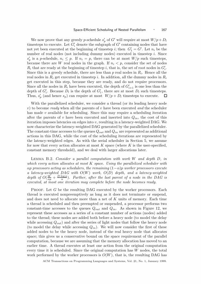
Space-Efficient Scheduling of Nested Parallelism · 167
We now prove that any greedy p-schedule s′p of G′ will require at most W/p+Dl
timesteps to execute. Let G′i denote the subgraph of G′ containing nodes that havenot yet been executed at the beginning of timestep i; then G′1 = G′. Let ni be thenumber of real nodes (not including dummy nodes) executed in timestep i. Sinces′p is a p-schedule, ni ≤ p. If ni = p, there can be at most W/p such timesteps,because there are W real nodes in the graph. If ni < p, consider the set of nodesRi that are ready at the beginning of timestep i, that is, the set of root nodes in G′i.Since this is a greedy schedule, there are less than p real nodes in Ri. Hence all thereal nodes in Ri get executed in timestep i. In addition, all the dummy nodes in Riget executed in this step, because they are ready, and do not require processors.Since all the nodes in Ri have been executed, the depth of G′i+1 is one less than thedepth of G′i. Because Dl is the depth of G′1, there are at most Dl such timesteps.Thus, s′p (and hence sp) can require at most W/p+Dl timesteps to execute.
With the parallelized scheduler, we consider a thread (or its leading heavy nodev) to become ready when all the parents of v have been executed and the schedulerhas made v available for scheduling. Since this may require a scheduling iterationafter the parents of v have been executed and inserted into Qin, the cost of thisiteration imposes latencies on edges into v, resulting in a latency-weighted DAG. Wenow characterize the latency-weighted DAG generated by the parallelized scheduler.The constant-time accesses to the queues Qout andQin are represented as additionalactions in this DAG, while the cost of the scheduling iterations are represented bythe latency-weighted edges. As with the serial scheduler in Section 5, we assumefor now that every action allocates at most K space (where K is the user-specified,constant memory threshold), and we deal with larger allocations later.
Lemma B.2. Consider a parallel computation with work W and depth D, inwhich every action allocates at most K space. Using the parallelized scheduler withαp processors acting as schedulers, the remaining (1−α)p worker processors executea latency-weighted DAG with O(W ) work, O(D) depth, and a latency-weighteddepth of O(Wαp + D·log p
α ). Further, after the last parent of a node in the DAG isexecuted, at most one iteration may complete before the node becomes ready.
Proof. Let G be the resulting DAG executed by the worker processors. Eachthread is executed nonpreemptively as long as it does not terminate or suspend,and does not need to allocate more than a net of K units of memory. Each timea thread is scheduled and then preempted or suspended, a processor performs twoconstant-time accesses to the queues Qout and Qin. As shown in Figure 12, werepresent these accesses as a series of a constant number of actions (nodes) addedto the thread; these nodes are added both before a heavy node (to model the delaywhile accessing Qout) and after the series of light nodes that follow the heavy node(to model the delay while accessing Qin). We will now consider the first of theseadded nodes to be the heavy node, instead of the real heavy node that allocatesspace; this gives us a conservative bound on the space requirement of the parallelcomputation, because we are assuming that the memory allocation has moved to anearlier time. A thread executes at least one action from the original computationevery time it is scheduled. Since the original computation has W nodes, the totalwork performed by the worker processors is O(W ), that is, the resulting DAG has
ACM Transactions on Programming Languages and Systems, Vol. 21, No. 1, January 1999.
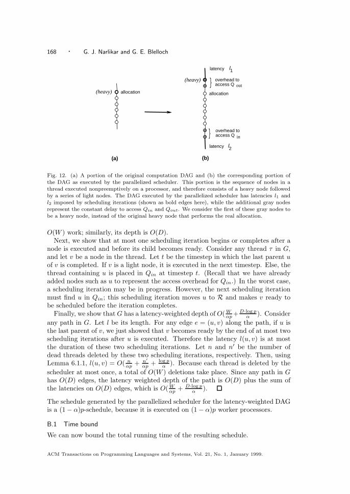
168 · G. J. Narlikar and G. E. Blelloch
allocation allocation
}latency 1
2
l
llatency
}
(heavy)
(heavy) overhead toaccess Q out
overhead toaccess Q in
(a) (b)
Fig. 12. (a) A portion of the original computation DAG and (b) the corresponding portion ofthe DAG as executed by the parallelized scheduler. This portion is the sequence of nodes in athread executed nonpreemptively on a processor, and therefore consists of a heavy node followedby a series of light nodes. The DAG executed by the parallelized scheduler has latencies l1 andl2 imposed by scheduling iterations (shown as bold edges here), while the additional gray nodesrepresent the constant delay to access Qin and Qout. We consider the first of these gray nodes tobe a heavy node, instead of the original heavy node that performs the real allocation.
O(W ) work; similarly, its depth is O(D).Next, we show that at most one scheduling iteration begins or completes after a
node is executed and before its child becomes ready. Consider any thread τ in G,and let v be a node in the thread. Let t be the timestep in which the last parent uof v is completed. If v is a light node, it is executed in the next timestep. Else, thethread containing u is placed in Qin at timestep t. (Recall that we have alreadyadded nodes such as u to represent the access overhead for Qin.) In the worst case,a scheduling iteration may be in progress. However, the next scheduling iterationmust find u in Qin; this scheduling iteration moves u to R and makes v ready tobe scheduled before the iteration completes.
Finally, we show that G has a latency-weighted depth of O(Wαp+D·log pα ). Consider
any path in G. Let l be its length. For any edge e = (u, v) along the path, if u isthe last parent of v, we just showed that v becomes ready by the end of at most twoscheduling iterations after u is executed. Therefore the latency l(u, v) is at mostthe duration of these two scheduling iterations. Let n and n′ be the number ofdead threads deleted by these two scheduling iterations, respectively. Then, usingLemma 6.1.1, l(u, v) = O( n
αp + n′
αp + log pα ). Because each thread is deleted by the
scheduler at most once, a total of O(W ) deletions take place. Since any path in Ghas O(D) edges, the latency weighted depth of the path is O(D) plus the sum ofthe latencies on O(D) edges, which is O(Wαp + D·log p
α ).
The schedule generated by the parallelized scheduler for the latency-weighted DAGis a (1− α)p-schedule, because it is executed on (1− α)p worker processors.
B.1 Time bound
We can now bound the total running time of the resulting schedule.
ACM Transactions on Programming Languages and Systems, Vol. 21, No. 1, January 1999.

Space-Efficient Scheduling of Nested Parallelism · 169
Lemma B.3. Consider a parallel computation with depth D and work W . Forany 0 < α < 1, when αp of the processors are dedicated to execute as schedulers,while the remaining act as worker processors, the parallel computation is executedin O( W
α(1−α)p + D·log pα ) time.
Proof. Let G be the DAG executed by the parallelized scheduler for this com-putation. We will show that the generated schedule sp of G is a greedy schedule,with O(W/p) additional timesteps in which the worker processors may be idle. Con-sider any scheduling iteration. Let ti be the timestep at which the ith schedulingiteration ends. After threads are inserted into Qout by the ith scheduling iteration,there are two possibilities:
(1) |Qout| < p log p. This implies that all the ready threads are in Qout, andno threads become ready until the end of the next scheduling iteration. Therefore,at every timestep j such that ti < j ≤ ti+1, if mj processors become idle and rjthreads are ready, min(mj , rj) threads are scheduled on the processors. (Recall thatwe have already added nodes to the DAG G to model the overheads of accessingQin and Qout.)
(2) |Qout| = p log p. Since (1− α)p worker processors will require at least log p(1−α)
timesteps to execute p log p actions, none of the worker processors will be idle forthe first log p
(1−α) steps after ti. However, if the (i+ 1)th scheduling iteration, which iscurrently executing, has to delete ni+1 dead threads, it may execute for O(ni+1
αp +log pα ) timesteps (using Lemma 6.1.1). Thus, in the worst case, the processors will
be busy for log p(1−α) steps and then remain idle for another O(ni+1
αp + log pα ) steps,
until the next scheduling iteration ends. We call such timesteps idling timesteps.Of the O(ni+1
αp + log pα ) idling steps, Θ( log p
α ) steps are within a factor of c(1−α)α of
the preceding log p(1−α) steps when all worker processors were busy (for some constant
c); therefore, they can add up to O(Wp ·(1−α)α ) = O(Wαp ). In addition, because
each thread is deleted only once, at most W threads can be deleted. Therefore, ifthe (i + 1)th scheduling iteration results in an additional O(ni+1
αp ) idle steps, theyadd up to O(Wαp ) idle steps over all the scheduling iterations. Therefore, a totalof O(Wαp ) idling steps can result due to the scheduler.
All timesteps besides the idling steps caused by the scheduler obey the conditionsrequired to make it a greedy (1−α)p-schedule, and therefore add up to O( W
(1−α)p +Wαp + D log p
α ) (using Lemmas B.1 and B.2). Along with the additional O(Wαp ) idlingsteps, the schedule requires a total of O( W
α(1−α)p + D·log pα ) timesteps.
Because α is a constant, that is, a constant fraction of the processors are dedicatedto the task of scheduling, the running time reduces to O(W/p+ D log p); here p isthe total number of processors, including both the schedulers and the workers.
B.2 Space bound
We now show that the total space requirement of the parallel schedule exceeds theserial schedule by O(D · p · log p). We first bound the number of premature nodesthat may exist in any prefix of the parallel schedule, and then bound the spacerequired to store threads in the three scheduling queues.
ACM Transactions on Programming Languages and Systems, Vol. 21, No. 1, January 1999.
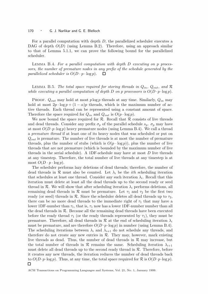
170 · G. J. Narlikar and G. E. Blelloch
For a parallel computation with depth D, the parallelized scheduler executes aDAG of depth O(D) (using Lemma B.2). Therefore, using an approach similarto that of Lemma 5.1.1, we can prove the following bound for the parallelizedscheduler.
Lemma B.4. For a parallel computation with depth D executing on p proces-sors, the number of premature nodes in any prefix of the schedule generated by theparallelized scheduler is O(D · p · log p).
Lemma B.5. The total space required for storing threads in Qin, Qout, and Rwhile executing a parallel computation of depth D on p processors is O(D ·p · log p).
Proof. Qout may hold at most p log p threads at any time. Similarly, Qin mayhold at most 2p · log p+ (1− α)p threads, which is the maximum number of ac-tive threads. Each thread can be represented using a constant amount of space.Therefore the space required for Qin and Qout is O(p · log p).
We now bound the space required for R. Recall that R consists of live threadsand dead threads. Consider any prefix σp of the parallel schedule sp. σp may haveat most O(D ·p · log p) heavy premature nodes (using Lemma B.4). We call a threada premature thread if at least one of its heavy nodes that was scheduled or put onQout is premature. The number of live threads is at most the number of prematurethreads, plus the number of stubs (which is O(p · log p)), plus the number of livethreads that are not premature (which is bounded by the maximum number of livethreads in the serial schedule). A 1DF-schedule may have at most D live threadsat any timestep. Therefore, the total number of live threads at any timestep is atmost O(D · p · log p).
The scheduler performs lazy deletions of dead threads; therefore, the number ofdead threads in R must also be counted. Let λi be the ith scheduling iterationthat schedules at least one thread. Consider any such iteration λi. Recall that thisiteration must delete at least all the dead threads up to the second ready or seedthread in R. We will show that after scheduling iteration λi performs deletions, allremaining dead threads in R must be premature. Let τ1 and τ2 be the first twoready (or seed) threads in R. Since the scheduler deletes all dead threads up to τ2,there can be no more dead threads to the immediate right of τ1 that may have alower 1DF-number than τ1, that is, τ1 now has a lower 1DF-number number than allthe dead threads in R. Because all the remaining dead threads have been executedbefore the ready thread τ1 (or the ready threads represented by τ1), they must bepremature. Therefore, all dead threads in R at the end of scheduling iteration λimust be premature, and are therefore O(D ·p · log p) in number (using Lemma B.4).The scheduling iterations between λi and λi+1 do not schedule any threads, andtherefore do not create any new entries in R. They may, however, mark existinglive threads as dead. Thus, the number of dead threads in R may increase, butthe total number of threads in R remains the same. Scheduling iteration λi+1
must delete all dead threads up to the second ready thread in R. Therefore, beforeit creates any new threads, the iteration reduces the number of dead threads backto O(D ·p · log p). Thus, at any time, the total space required for R is O(D ·p · log p).
ACM Transactions on Programming Languages and Systems, Vol. 21, No. 1, January 1999.
Space-Efficient Scheduling of Nested Parallelism · 171
Since every premature node may allocate at most K space, we can now state thefollowing space bound using Lemmas B.4 and B.5.
Lemma B.6. A parallel computation with work W and depth D, in which everynode allocates at most K space, and which requires S1 space to execute on oneprocessor, can be executed on p processors in S1 +O(K ·D ·p · logp) space (includingscheduler space) using the parallelized scheduler.
As in Section 5, allocations larger than K units are handled by delaying theallocation with parallel dummy threads. If Sa is the total space allocated, thenumber of dummy nodes added is at most Sa/K, and the depth is increased by aconstant factor. Therefore, using the parallelized scheduler, the final time bound ofO(W/p+Sa/pK +D · log p) and the space bound of S1 +O(K ·D · p · log p) follow,as stated in Theorem 6.2.1. These bounds include the scheduler overheads.
ACKNOWLEDGMENTS
Access to the SGI Power Challenge was provided by the the National Center forSupercomputing Applications (NCSA), whose staff was extremely helpful whendealing with all our requests
REFERENCES
Arvind, Nikhil, R. S., and Pingali, K. 1989. I-structures: Data structures for parallel computing.ACM Trans. on Programm. Lang. Syst. 11, 4 (Oct.), 598–632.
Bershad, B. N., Lazowska, E., and Levy, H. 1988. PRESTO : A system for object-orientedparallel programming. Soft. Pract. and Exper. 18, 8 (Aug.), 713–732.
Blelloch, G. E., Chatterjee, S., Hardwick, J. C., Sipelstein, J., and Zagha, M. 1994.Implementation of a portable nested data-parallel language. Journal of Parallel and DistributedComputing 21, 1 (April), 4–14.
Blelloch, G. E., Gibbons, P. B., and Matias, Y. 1995. Provably efficient scheduling for lan-guages with fine-grained parallelism. In Proc. Symposium on Parallel Algorithms and Archi-tectures, Santa Barbara, pp. 420–430.
Blumofe, R. D., Frigo, M., Joerg, C. F., Leiserson, C. E., and Randall, K. H. 1996. AnAnalysis of Dag-Consistent Distributed Shared-Memory Algorithms. In Proc. Symp. on ParallelAlgorithms and Architectures, pp. 297–308.
Blumofe, R. D., Joerg, C. F., Kuszmaul, B. C., Leiserson, C. E., Randall, K. H., and Zhou,
Y. 1995. Cilk: An efficient multithreaded runtime system. In Proc. Symposium on Principlesand Practice of Parallel Programming, pp. 207–216.
Blumofe, R. D. and Leiserson, C. E. 1993. Space-efficient scheduling of multithreaded compu-tations. In Proc. 25th ACM Symp. on Theory of Computing, pp. 362–371.
Blumofe, R. D. and Leiserson, C. E. 1994. Scheduling multithreaded computations by workstealing. In Proc. 35th IEEE Symp. on Foundations of Computer Science, pp. 356–368.
Burton, F. W. 1988. Storage management in virtual tree machines. IEEE Trans. on Comput-ers 37, 3, 321–328.
Burton, F. W. and Simpson, D. J. 1994. Space efficient execution of deterministic parallel
programs. Manuscript.
Burton, F. W. and Sleep, M. R. 1981. Executing functional programs on a virtual tree ofprocessors. In Conference on Functional Programming Languages and Computer Architecture.
Chandra, R., Gupta, A., and Hennessy, J. 1994. COOL: An object-based language for parallelprogramming. IEEE Computer 27, 8 (Aug.), 13–26.
Chandy, K. M. and Kesselman, C. 1992. Compositional c++: compositional parallel program-ming. In Proc. 5th. Intl. Wkshp. on Languages and Compilers for Parallel Computing, NewHaven, CT, pp. 124–144.
ACM Transactions on Programming Languages and Systems, Vol. 21, No. 1, January 1999.
172 · G. J. Narlikar and G. E. Blelloch
Chase, J. S., Amador, F. G., and Lazowska, E. D. 1989. The amber system: Parallel program-ming on a network of multiprocessors. In Proc. Symposium on Operating Systems Principles.
Chow, J. H. and W. L. Harrison 1990. Switch-stacks: A scheme for microtasking nested parallelloops. In Proc. Supercomputing, New York, NY.
Cook, S. A. 1985. A taxonomy of problems with fast parallel algorithms. Information andControl 64, 2–22.
Culler, D. E. and Arvind 1988. Resource requirements of dataflow programs. In Proc. Intl.Symposium on Computer Architecture.
Feo, J. T., Cann, D. C., and Oldehoeft, R. R. 1990. A report on the Sisal language project.Journal of Parallel and Distributed Computing 10, 4 (Dec.), 349–366.
Freeh, V. W., Lowenthal, D. K., and Andrews, G. R. 1994. Distributed filaments: efficientfine-grain parallelism on a cluster of workstations. In 1st Symposium on Operating SystemsDesign and Implementation, Monterey, CA, pp. 201–212.
Goldstein, S. C., Culler, D. E., and Schauser, K. E. 1995. Enabling primitives for compilingparallel languages. In 3rd Workshop on Languages, Compilers, and Run-Time Systems forScalable Computers, Rochester, NY.
Greengard, L. 1987. The rapid evaluation of potential fields in particle systems. The MIT Press.
Halbherr, M., Zhou, Y., and Joerg, C. F. 1994. Parallel programming based on continuation-passing thread. In Proc. 2nd International Workshop on Massive Parallelism: Hardware, Soft-ware and Applications, Capri, Italy.
Halstead, R. H. 1985. Multilisp: A language for concurrent symbolic computation. ACM Trans.on Programming Languages and Systems 7, 4, 501–538.
HPF Forum 1993. High Performance Fortran language specification, Version 1.0.
Hseih, W. E., Wang, P., and Weihl, W. E. 1993. Computation migration: enhancing localityfor distributed memory parallel systems. In Proc. Symposium on Principles and Practice ofParallel Programming, San Francisco, California.
Hummel, S. F. and Schonberg, E. 1991. Low-overhead scheduling of nested parallelsim. IBMJournal of Research and Development 35, 5-6, 743–65.
Hummel, S. F., Schonberg, E., and Flynn, L. E. 1992. Factoring: a method for schedulingparallel loops. Commun. ACM 35, 8 (Aug.), 90–101.
IEEE 1985. Threads extension for portable operating systems (draft 6).
Kuck, C. D. P. D. 1987. Guided self-scheduling: a practical scheduling scheme for parallelsupercomputers. IEEE Trans. on Computers C-36, 12 (Dec.), 1425–39.
Mellor-Crummey, J. M. 1987. Concurrent queues: Practical Fetch-and-Φ algorithms. TechnicalReport 229 (Nov.), University of Rochester.
Mills, P. H., Nyland, L. S., Prins, J. F., Reif, J. H., and Wagner, R. A. 1990. Prototypingparallel and distributed programs in Proteus. Technical Report UNC-CH TR90-041, ComputerScience Department, University of North Carolina.
Mohr, E., Kranz, D., and Halstead, R. 1991. Lazy task creation: A technique for increasingthe granularity of parallel programs. IEEE Trans. on Parallel and Distributed Systems 2, 3(July), 264–280.
Mueller, F. 1993. A library implementation of POSIX threads under unix. In Proc. Winter1993 USENIX Technical Conference and Exhibition, San Diego, CA, USA, pp. 29–41.
Narlikar, G. J. 1999. Space-efficient multithreading. School of Computer Science, CarnegieMellon University. Ph.D. thesis, to appear.
Narlikar, G. J. and Blelloch, G. E. 1996. A framework for space and time efficient schedulingof parallelism. Technical Report CMU-CS-96-197, Computer Science Department, CarnegieMellon University.
Narlikar, G. J. and Blelloch, G. E. 1998. Pthreads for dynamic and irregular parallelism. InProc. SC98: High Performance Networking and Computing, Orlando, FL. IEEE.
Nikhil, R. S. 1994. Cid: A parallel, shared-memory c for distributed memory machines. In Proc.7th. Ann. Wkshp. on Languages and Compilers for Parallel Computing, pp. 376–390.
ACM Transactions on Programming Languages and Systems, Vol. 21, No. 1, January 1999.

Space-Efficient Scheduling of Nested Parallelism · 173
Powell, M. L., Kleiman, S. R., Barton, S., Shah, D., Stein, D., and Weeks, M. 1991. SunOSmulti-thread architecture. In USENIX Association (Ed.), Proc. Winter 1991 USENIX Con-ference: Dallas, TX, USA, pp. 65–80.
Quinlan, J. R. 1986. Induction of decision trees. Machine learning 1, 1, 81–106.
Rinard, M. C., Scales, D. J., and Lam, M. S. 1993. Jade: A high-level, machine-independentlanguage for parallel programming. IEEE Computer 26, 6 (June), 28–38.
Rogers, A., Carlisle, M., Reppy, J., and Hendren, L. 1995. Supporting dynamic data struc-tures on distributed memory machines. ACM Trans. on Programm. Lang. Syst. 17, 2 (March),233–263.
Rugguero, C. A. and Sargeant, J. 1987. Control of parallelism in the manchester dataflowmachine. In Functional Programming Languages and Computer Architecture, Volume 174 ofLecture Notes in Computer Science, pp. 1–15. Springer-Verlag.
Strassen, V. 1969. Gaussian elimination is not optimal. Numerische Mathematik 13, 354–356.
Tzen, T. H. and Ni, L. M. 1993. Trapezoid self-scheduling: a practical scheduling scheme forparallel compilers. IEEE Trans. on Parallel and Distributed Systems 4, 1 (Jan.), 87–98.
Vandevoorde, M. T. and Roberts, E. S. 1988. WorkCrews: an abstraction for controllingparallelism. International Journal of Parallel Programming 17, 4 (Aug.), 347–366.
Received May 1998; accepted November 1998
ACM Transactions on Programming Languages and Systems, Vol. 21, No. 1, January 1999.