Embed Size (px)
Citation preview

2
Space-Time Coding PerformanceAnalysis and Code Design
2.1 Introduction
In Chapter 1, we showed that the information capacity of wireless communication systemscan be increased considerably by employing multiple transmit and receive antennas. For asystem with a large number of transmit and receive antennas and an independent flat fadingchannel known at the receivers, the capacity grows linearly with the minimum number ofantennas.
An effective and practical way to approaching the capacity of multiple-input multiple-output (MIMO) wireless channels is to employ space-time (ST) coding [6]. Space-timecoding is a coding technique designed for use with multiple transmit antennas. Coding isperformed in both spatial and temporal domains to introduce correlation between signalstransmitted from various antennas at various time periods. The spatial-temporal correla-tion is used to exploit the MIMO channel fading and minimize transmission errors at thereceiver. Space-time coding can achieve transmit diversity and power gain over spatiallyuncoded systems without sacrificing the bandwidth. There are various approaches in cod-ing structures, including space-time block codes (STBC), space-time trellis codes (STTC),space-time turbo trellis codes and layered space-time (LST) codes. A central issue in allthese schemes is the exploitation of multipath effects in order to achieve high spectralefficiencies and performance gains. In this chapter, we start with a brief review of fadingchannel models and diversity techniques. Then, we proceed with the analysis of the per-formance of space-time codes on fading channels. The analytical pairwise error probabilityupper bounds over Rician and Rayleigh channels with independent fading are derived. Theyare followed by the presentation of the code design criteria on slow and fast Rayleigh fadingchannels.
Space-Time Coding Branka Vucetic and Jinhong Yuanc© 2003 John Wiley & Sons, Ltd ISBN: 0-470-84757-3

50 Space-Time Coding Performance Analysis and Code Design
2.2 Fading Channel Models
2.2.1 Multipath Propagation
In a cellular mobile radio environment, the surrounding objects, such as houses, buildingor trees, act as reflectors of radio waves. These obstacles produce reflected waves withattenuated amplitudes and phases. If a modulated signal is transmitted, multiple reflectedwaves of the transmitted signal will arrive at the receiving antenna from different directionswith different propagation delays. These reflected waves are called multipath waves [47].Due to the different arrival angles and times, the multipath waves at the receiver site havedifferent phases. When they are collected by the receiver antenna at any point in space, theymay combine either in a constructive or a destructive way, depending on the random phases.The sum of these multipath components forms a spatially varying standing wave field. Themobile unit moving through the multipath field will receive a signal which can vary widelyin amplitude and phase. When the mobile unit is stationary, the amplitude variations inthe received signal are due to the movement of surrounding objects in the radio channel.The amplitude fluctuation of the received signal is called signal fading. It is caused by thetime-variant multipath characteristics of the channel.
2.2.2 Doppler Shift
Due to the relative motion between the transmitter and the receiver, each multipath waveis subject to a shift in frequency. The frequency shift of the received signal caused by therelative motion is called the Doppler shift. It is proportional to the speed of the mobile unit.Consider a situation when only a single tone of frequency fc is transmitted and a receivedsignal consists of only one wave coming at an incident angle θ with respect to the directionof the vehicle motion. The Doppler shift of the received signal, denoted by fd , is given by
fd = vfc
ccos θ (2.1)
where v is the vehicle speed and c is the speed of light. The Doppler shift in a multipathpropagation environment spreads the bandwidth of the multipath waves within the range offc ± fdmax , where fdmax is the maximum Doppler shift, given by
fdmax = vfc
c(2.2)
The maximum Doppler shift is also referred as the maximum fade rate. As a result, a singletone transmitted gives rise to a received signal with a spectrum of nonzero width. Thisphenomenon is called frequency dispersion of the channel.
2.2.3 Statistical Models for Fading Channels
Because of the multiplicity of factors involved in propagation in a cellular mobile environ-ment, it is convenient to apply statistical techniques to describe signal variations.
In a narrowband system, the transmitted signals usually occupy a bandwidth smallerthan the channel’s coherence bandwidth, which is defined as the frequency range overwhich the channel fading process is correlated. That is, all spectral components of thetransmitted signal are subject to the same fading attenuation. This type of fading is referred

Fading Channel Models 51
to as frequency nonselective or frequency flat. On the other hand, if the transmitted signalbandwidth is greater than the channel coherence bandwidth, the spectral components ofthe transmitted signal with a frequency separation larger than the coherence bandwidth arefaded independently. The received signal spectrum becomes distorted, since the relationshipsbetween various spectral components are not the same as in the transmitted signal. Thisphenomenon is known as frequency selective fading. In wideband systems, the transmittedsignals usually undergo frequency selective fading.
In this section we introduce Rayleigh and Rician fading models to describe signal varia-tions in a narrowband multipath environment. The frequency selective fading models for awideband system are addressed in Chapter 8.
Rayleigh Fading
We consider the transmission of a single tone with a constant amplitude. In a typical landmobile radio channel, we may assume that the direct wave is obstructed and the mobile unitreceives only reflected waves. When the number of reflected waves is large, according tothe central limit theorem, two quadrature components of the received signal are uncorrelatedGaussian random processes with a zero mean and variance σ 2
s . As a result, the envelopeof the received signal at any time instant undergoes a Rayleigh probability distribution andits phase obeys a uniform distribution between −π and π . The probability density function(pdf) of the Rayleigh distribution is given by
p(a) ={
a
σ 2s
· e−a2/2σ 2s a ≥ 0
0 a < 0(2.3)
The mean value, denoted by ma , and the variance, denoted by σ 2a , of the Rayleigh distributed
random variable are given by
ma = √π2 · σs = 1.2533σs
σ 2a = (2 − π
2
)σ 2
s = 0.4292σ 2s
(2.4)
If the probability density function in (2.3) is normalized so that the average signal power(E[a2]) is unity, then the normalized Rayleigh distribution becomes
p(a) ={
2ae−a2a ≥ 0
0 a < 0(2.5)
The mean value and the variance are
ma = 0.8862σ 2
a = 0.2146(2.6)
The pdf for a normalized Rayleigh distribution is shown in Fig. 2.1.In fading channels with a maximum Doppler shift of fdmax , the received signal experiences
a form of frequency spreading and is band-limited between fc ± fdmax . Assuming an omni-directional antenna with waves arriving in the horizontal plane, a large number of reflectedwaves and a uniform received power over incident angles, the power spectral density of thefaded amplitude, denoted by |P (f )|, is given by
|P (f )| =
1
2π
√f 2
dmax−f 2
if |f | ≤ |fdmax |0 otherwise
(2.7)

52 Space-Time Coding Performance Analysis and Code Design
0 0.5 1 1.5 2 2.5 30
0.1
0.2
0.3
0.4
0.5
0.6
0.7
0.8
0.9
a
p(a)
Figure 2.1 The pdf of Rayleigh distribution
where f is the frequency and fdmax is the maximum fade rate. The value of fdmaxTs is themaximum fade rate normalized by the symbol rate. It serves as a measure of the channelmemory. For correlated fading channels this parameter is in the range 0 < fdmaxTs < 1,indicating a finite channel memory. The autocorrelation function of the fading process isgiven by
R(τ) = J0(2πfdmaxτ
)(2.8)
where J0(·) is the zero-order Bessel function of the first kind.
Rician Fading
In some propagation scenarios, such as satellite or microcellular mobile radio channels,there are essentially no obstacles on the line-of-sight path. The received signal consists ofa direct wave and a number of reflected waves. The direct wave is a stationary nonfadingsignal with a constant amplitude. The reflected waves are independent random signals. Theirsum is called the scattered component of the received signal.
When the number of reflected waves is large, the quadrature components of the scatteredsignal can be characterized as a Gaussian random process with a zero mean and varianceσ 2
s . The envelope of the scattered component has a Rayleigh probability distribution.The sum of a constant amplitude direct signal and a Rayleigh distributed scattered signal
results in a signal with a Rician envelope distribution. The pdf of the Rician distribution isgiven by
p(a) = a
σ 2se− (a2+D2)
2σ2s I0
(aD
σ 2s
)a ≥ 0
0 a < 0(2.9)

Fading Channel Models 53
where D2 is the direct signal power and I0(·) is the modified Bessel function of the firstkind and zero-order.
Assuming that the total average signal power is normalized to unity, the pdf in (2.9)becomes
p(a) ={
2a(1 + K)e−K−(1+K)a2I0(2a
√K(K + 1)
)a ≥ 0
0 a < 0
where K is the Rician factor, denoting the power ratio of the direct and the scattered signalcomponents. The Rician factor is given by
K = D2
2σ 2s
(2.10)
The mean and the variance of the Rician distributed random variable are given by
ma = 12
√π
1+Ke− K
2
[(1+K)I0
(K2
)+KI1
(K2
)]
σ 2a = 1 − m2
a
(2.11)
where I1(·) is the first order modified Bessel function of the first kind. Small values of K
indicate a severely faded channel. For K = 0, there is no direct signal component and theRician pdf becomes a Rayleigh pdf. On the other hand, large values of K indicate a slightlyfaded channel. For K approaching infinity, there is no fading at all resulting in an AWGNchannel. The Rician distributions with various K are shown in Fig. 2.2.
These two models can be applied to describe the received signal amplitude variationswhen the signal bandwidth is much smaller than the coherence bandwidth.
0 0.5 1 1.5 2 2.5 30
0.2
0.4
0.6
0.8
1
1.2
1.4
1.6
1.8
2
a
p(a)
K=0K=2K=5K=10
Figure 2.2 The pdf of Rician distributions with various K

54 Space-Time Coding Performance Analysis and Code Design
2.3 Diversity
2.3.1 Diversity TechniquesIn wireless mobile communications, diversity techniques are widely used to reduce theeffects of multipath fading and improve the reliability of transmission without increas-ing the transmitted power or sacrificing the bandwidth [49] [48]. The diversity techniquerequires multiple replicas of the transmitted signals at the receiver, all carrying the sameinformation but with small correlation in fading statistics. The basic idea of diversity is that,if two or more independent samples of a signal are taken, these samples will fade in anuncorrelated manner, e.g., some samples are severely faded while others are less attenuated.This means that the probability of all the samples being simultaneously below a given levelis much lower than the probability of any individual sample being below that level. Thus,a proper combination of the various samples results in greatly reduced severity of fading,and correspondingly, improved reliability of transmission.
In most wireless communication systems a number of diversity methods are used in orderto get the required performance. According to the domain where diversity is introduced,diversity techniques are classified into time, frequency and space diversity.
Time Diversity
Time diversity can be achieved by transmitting identical messages in different time slots,which results in uncorrelated fading signals at the receiver. The required time separation isat least the coherence time of the channel, or the reciprocal of the fading rate 1/fd = c/vfc.The coherence time is a statistical measure of the period of time over which the channelfading process is correlated. Error control coding is regularly used in digital communicationsystems to provide a coding gain relative to uncoded systems. In mobile communications,error control coding is combined with interleaving to achieve time diversity. In this case,the replicas of the transmitted signals are usually provided to the receiver in the form ofredundancy in the time domain introduced by error control coding [15]. The time separationbetween the replicas of the transmitted signals is provided by time interleaving to obtainindependent fades at the input of the decoder. Since time interleaving results in decodingdelays, this technique is usually effective for fast fading environments where the coher-ence time of the channel is small. For slow fading channels, a large interleaver can leadto a significant delay which is untolerable for delay sensitive applications such as voicetransmission. This constraint rules out time diversity for some mobile radio systems. Forexample, when a mobile radio station is stationary, time diversity cannot help to reducefades. One of the drawbacks of the scheme is that due to the redundancy introduced in thetime domain, there is a loss in bandwidth efficiency.
Frequency Diversity
In frequency diversity, a number of different frequencies are used to transmit the same mes-sage. The frequencies need to be separated enough to ensure independent fading associatedwith each frequency. The frequency separation of the order of several times the chan-nel coherence bandwidth will guarantee that the fading statistics for different frequenciesare essentially uncorrelated. The coherence bandwidth is different for different propagationenvironments. In mobile communications, the replicas of the transmitted signals are usuallyprovided to the receiver in the form of redundancy in the frequency domain introduced by

Diversity 55
spread spectrum such as direct sequence spread spectrum (DSSS), multicarrier modulationand frequency hopping. Spread spectrum techniques are effective when the coherence band-width of the channel is small. However, when the coherence bandwidth of the channel islarger than the spreading bandwidth, the multipath delay spread will be small relative to thesymbol period. In this case, spread spectrum is ineffective to provide frequency diversity.Like time diversity, frequency diversity induces a loss in bandwidth efficiency due to aredundancy introduced in the frequency domain.
Space Diversity
Space diversity has been a popular technique in wireless microwave communications. Spacediversity is also called antenna diversity. It is typically implemented using multiple antennasor antenna arrays arranged together in space for transmission and/or reception. The mul-tiple antennas are separated physically by a proper distance so that the individual signalsare uncorrelated. The separation requirements vary with antenna height, propagation envi-ronment and frequency. Typically a separation of a few wavelengths is enough to obtainuncorrelated signals. In space diversity, the replicas of the transmitted signals are usuallyprovided to the receiver in the form of redundancy in the space domain. Unlike time andfrequency diversity, space diversity does not induce any loss in bandwidth efficiency. Thisproperty is very attractive for future high data rate wireless communications.
Polarization diversity and angle diversity are two examples of space diversity. In polar-ization diversity, horizontal and vertical polarization signals are transmitted by two differentpolarized antennas and received by two different polarized antennas. Different polarizationsensure that the two signals are uncorrelated without having to place the two antennas farapart [15]. Angle diversity is usually applied for transmissions with carrier frequency largerthan 10 GHz. In this case, as the transmitted signals are highly scattered in space, thereceived signals from different directions are independent to each other. Thus, two or moredirectional antennas can be pointed in different directions at the receiver site to provideuncorrelated replicas of the transmitted signals [52].
Depending on whether multiple antennas are used for transmission or reception, we canclassify space diversity into two categories: receive diversity and transmit diversity [40].In receive diversity, multiple antennas are used at the receiver site to pick up independentcopies of the transmit signals. The replicas of the transmitted signals are properly combinedto increase the overall received SNR and mitigate multipath fading. In transmit diversity,multiple antennas are deployed at the transmitter site. Messages are processed at the trans-mitter and then spread across multiple antennas. The details of transmit diversity is discussedin Section 2.3.3.
In practical communication systems, in order to meet the system performance require-ments, two or more conventional diversity schemes are usually combined to provide multi-dimensional diversity [48]. For example, in GSM cellular systems multiple receive anten-nas at base stations are used in conjunction with interleaving and error control coding tosimultaneously exploit both space and time diversity.
2.3.2 Diversity Combining Methods
In the previous section, diversity techniques were classified according to the domain wherethe diversity is introduced. The key feature of all diversity techniques is a low probability

56 Space-Time Coding Performance Analysis and Code Design
of simultaneous deep fades in various diversity subchannels. In general, the performance ofcommunication systems with diversity techniques depends on how multiple signal replicasare combined at the receiver to increase the overall received SNR. Therefore, diversityschemes can also be classified according to the type of combining methods employed atthe receiver. According to the implementation complexity and the level of channel stateinformation required by the combining method at the receiver, there are four main typesof combining techniques, including selection combining, switched combining, equal-gaincombining (EGC) and maximal ratio combining (MRC) [48] [49].
Selection Combining
Selection combining is a simple diversity combining method. Consider a receive diversitysystem with nR receive antennas. The block diagram of the selection combining scheme isshown in Fig. 2.3. In such a system, the signal with the largest instantaneous signal-to-noiseratio (SNR) at every symbol interval is selected as the output, so that the output SNR isequal to that of the best incoming signal. In practice, the signal with the highest sum of thesignal and noise power (S + N) is usually used, since it is difficult to measure the SNR.
Switched Combining
In a switched combining diversity system as shown in Fig. 2.4, the receiver scans all thediversity branches and selects a particular branch with the SNR above a certain prede-termined threshold. This signal is selected as the output, until its SNR drops below thethreshold. When this happens, the receiver starts scanning again and switches to anotherbranch. This scheme is also called scanning diversity.
Compared to selection diversity, switched diversity is inferior since it does not continuallypick up the best instantaneous signal. However, it is simpler to implement as it does notrequire simultaneous and continuous monitoring of all the diversity branches [50].
For both the selection and switched diversity schemes, the output signal is equal to onlyone of all the diversity branches. In addition, they do not require any knowledge of channelstate information. Therefore, these two schemes can be used in conjunction with coherentas well as noncoherent modulations [48].
r1 r2 rnR
� � �
�
RFFront End
RFFront End
RFFront End
Logic Selector
output
���� ���� ����
Rx 1 Rx 2
· · ·
Rx nR
Figure 2.3 Selection combining method
Diversity 57
r1 r2 rnR
� � �
�
RFFront End
RFFront End
RFFront End
Scan and Switch Unit
output
���� ���� ����
Rx 1 Rx 2
· · ·
Rx nR
Figure 2.4 Switched combining method
r1 r2 rnR
� � �
�
�
RFFront End
RFFront End
RFFront End
� � �× × ×� � �α1 α2 αnR
+
Output
Detector
���� ���� ����
Rx 1 Rx 2
· · ·
Rx nR
Figure 2.5 Maximum ratio combining method
Maximal Ratio Combining
Maximum ratio combining is a linear combining method. In a general linear combiningprocess, various signal inputs are individually weighted and added together to get an outputsignal. The weighting factors can be chosen in several ways.
Figure 2.5 shows a block diagram of a maximum ratio combining diversity. The outputsignal is a linear combination of a weighted replica of all of the received signals. It is
58 Space-Time Coding Performance Analysis and Code Design
given by
r =nR∑i=1
αi · ri (2.12)
where ri is the received signal at receive antenna i, and αi is the weighting factor for receiveantenna i. In maximum ratio combining, the weighting factor of each receive antenna ischosen to be in proportion to its own signal voltage to noise power ratio. Let Ai and φi bethe amplitude and phase of the received signal ri , respectively. Assuming that each receiveantenna has the same average noise power, the weighting factor αi can be represented as
αi = Aie−jφi (2.13)
This method is called optimum combining since it can maximize the output SNR. It isshown that the maximum output SNR is equal to the sum of the instantaneous SNRs of theindividual signals [49].
In this scheme, each individual signal must be co-phased, weighted with its correspond-ing amplitude and then summed. This scheme requires the knowledge of channel fadingamplitude and signal phases. So, it can be used in conjunction with coherent detection, butit is not practical for noncoherent detection [48].
Equal Gain Combining
Equal gain combining is a suboptimal but simple linear combining method. It does notrequire estimation of the fading amplitude for each individual branch. Instead, the receiversets the amplitudes of the weighting factors to be unity.
αi = e−jφi (2.14)
In this way all the received signals are co-phased and then added together with equal gain.The performance of equal-gain combining is only marginally inferior to maximum ratiocombining. The implementation complexity for equal-gain combining is significantly lessthan the maximum ratio combining.
Example 2.1
In order to illustrate the effects of multipath fading on system error performance, we consideran uncoded BPSK system with and without multipath fading.
The bit error probability of BPSK signals on AWGN channels with coherent detection isgiven by [47]
Pb(e) = Q
(√2Eb
N0
)(2.15)
where Eb
N0is the ratio of the bit energy to the noise power spectral density.
In a fading channel, we assume that a fading coefficient is constant within each signallinginterval so that coherent detection can be achieved. For a given fading attenuation a, theconditional bit error probability of coherent BPSK signals is given by
Pb(e|a) = Q(√
2γb
)(2.16)
Diversity 59
where γb = a2 Eb
N0is the received SNR per bit. To obtain the average error probability when
a is random, we need to average (2.16) over the probability density function of γb. Let usdefine the average SNR per bit as
γ b = E(a2)Eb
N0(2.17)
where E(·) denotes the expectation operation. For a Rayleigh fading channel, the averagebit error probability of BPSK signals is given by [47]
Pb(e) = 1
2
(1 −
√γ b
1 + γ b
)(2.18)
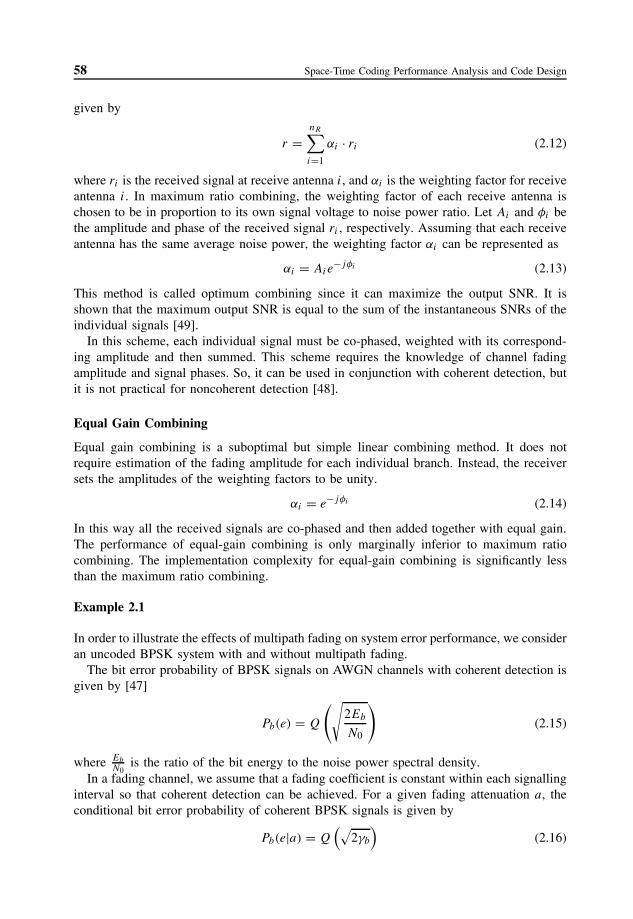
In order to compare the performance of the coherent BPSK signalling on channels with andwithout fading, we plot the bit error probabilities (2.15) and (2.18) in Fig. 2.6. From thefigure, we can observe that the error rate decreases exponentially with the increasing SNRfor a nonfading channel. However, for a Rayleigh fading channel, the error rate decreasesinversely with the SNR. In order to achieve the same bit error rate of 10−4, the requiredtransmission power for a fading channel must increase by more than 25 dB relative to thatfor a nonfading channel due to the impairment of the multipath fading.
To show the effectiveness of the diversity techniques in combating the multipath fading,we consider an uncoded BPSK system with receive diversity on fading channels in thefollowing example.
Let us assume that the receiver employs nR receive antennas. The transmitted BPSKsignals are received over nR independent and identically distributed (i.i.d.) Rayleigh fadingchannels corrupted by AWGN. The nR received signals are combined by using an MRC
0 5 10 15 20 25 30 35 40 4510
−5
10−4
10−3
10−2
10−1
100
Eb/No (dB)
BER
AWGNFading
Figure 2.6 BER performance comparison of coherent BPSK on AWGN and Rayleigh fadingchannels
60 Space-Time Coding Performance Analysis and Code Design
method. Let γ k = E[γk] be the average value of SNR per bit on the k-th channel. Forindependent and identically distributed channels, γ = γ k . The average SNR per bit afterthe MRC is nRγ . The average bit error probability of the coherent BPSK with nR receiveantennas and MRC diversity on Rayleigh i.i.d. fading channels is given by [47]
Pb(e) =[
1
2
(1 −
√γ
1 + γ
)]nR nR−1∑k=0
(nR − 1 + k
k
)[1
2
(1 +
√γ
1 + γ
)]k
(2.19)
When the average SNR on each diversity channel is high, the above average bit errorprobability can be approximated as
Pb(e) ≈(
1
4γ
)nR(
2nR − 1nR
)(2.20)
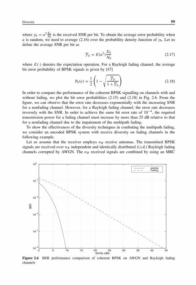
The bit error rate curves for various numbers of receive antennas nR are depicted in Fig. 2.7.The receive antenna diversity dramatically improves the error performance compared to thecase without diversity (nR = 1). In particular, we observe that the error probability decreasesinversely with the nR-th power of the SNR. For the same error rate of 10−4, the MRC receivediversity technique reduces the transmission power by about 17 dB, 6 dB, 3 dB, 2 dB and1.6 dB, when the number of receive antennas is increased from one to six successively.
2.3.3 Transmit Diversity
In present cellular mobile communications systems multiple receive antennas are used forthe base stations with the aim to both suppress co-channel interference and minimize the
0 5 10 15 20 25 30 35 40 4510
−5
10−4
10−3
10−2
10−1
100
Eb/No (dB)
BER
Figure 2.7 BER performance of coherent BPSK on Rayleigh fading channels with MRC receivediversity; the top curve corresponds to the performance without diversity; the other lower curvescorrespond to systems with 2, 3, 4, 5 and 6 receive antennas, respectively, starting from the top

Diversity 61
fading effects. For example, in GSM and IS-136, multiple antennas are used at the basestation to create uplink (from mobiles to base stations) receive diversity, compensatingfor the relatively low transmission power from the mobile. This improves the quality andrange in the uplink. But for the downlink (from base stations to mobiles), it is difficultto utilize receive diversity at the mobile. Firstly, it is hard to place more than two anten-nas in a small-sized portable mobile. Secondly, multiple receive antennas imply multiplesets of RF down convertors and, as a result, more processing power, which is limited formobile units. For the downlink, it is more practical to consider transmit diversity. It is easyto install multiple transmit antennas in the base station and provide the extra power formultiple transmissions. Transmit diversity decreases the required processing power of thereceivers, resulting in a simpler system structure, lower power consumption and lower cost.Furthermore, transmit diversity can be combined with receive diversity to further improvethe system performance.
In contrast to receiver diversity which is widely applied in cellular mobile systems,transmit diversity has received little attention as the behavior of transmit antenna diversityis dramatically different from that of receive antenna diversity and it is more difficult toexploit transmit diversity [15]. The difficulties mainly include that: (1) since the transmittedsignals from multiple antennas are mixed spatially before they arrive at the receiver, someadditional signal processing is required at both the transmitter and the receiver in orderto separate the received signals and exploit diversity; and (2) unlike the receiver that canusually estimate fading channels, the transmitter does not have instantaneous informationabout the channel unless the information is fed back from the receiver to the transmitter [40].
Transmit diversity can increase the channel capacity considerably as has been shown inChapter 1. A number of transmit diversity schemes have been proposed in the literature.These schemes can be divided into two categories: schemes with and without feedback.The difference between the two types of schemes is that the former relies on the channelinformation at the transmitter, which is obtained via feedback channels, while the latter doesnot require any channel information at the transmitter [6] [15] [40].
For transmit diversity systems with feedback, modulated signals are transmitted frommultiple transmit antennas with different weighting factors. The weighting factors for thetransmit antennas are chosen adaptively so that the received signal power or channel capacityis maximized. Switched diversity proposed in [16] is an example of such transmit diversityschemes. In practical cellular mobile systems, mobility and environment change cause fastchannel variations, making channel estimation and tracking difficult. The imperfect channelestimation and mismatch between the previous channel state and current channel conditionwill decrease the received signal SNR and affect the system performance.
For transmit diversity schemes without feedback, messages to be transmitted are usuallyprocessed at the transmitter and then sent from multiple transmit antennas. Signal processingat the transmitter is designed appropriately to enable the receiver exploiting the embeddeddiversity from the received signals. At the receiver, messages are recovered by using asignal detection technique. A typical example is a delay diversity scheme [17] [18] [19].In this scheme, copies of the same symbol are transmitted through multiple antennas indifferent times as shown in Fig. 2.8. At the receiver side, the delays of the second upto thenT -th transmit antennas introduce a multipath-like distortion for the signal transmitted fromthe first antenna. The multipath distortion can be resolved or exploited at the receiver byusing a maximum likelihood sequence estimator (MLSE) or a minimum mean square error(MMSE) equalizer to obtain a diversity gain. In some sense, the delay diversity is an optimal

62 Space-Time Coding Performance Analysis and Code Design
� �
�
�
delay(nT − 1)Ts
...
delayTs
ModulatorEncoder
����
����
����
Tx 2
Tx 1
Tx nT
Figure 2.8 Delay transmit diversity scheme
transmit diversity scheme since it can achieve the maximum possible transmit diversity orderdetermined by the number of transmit antennas without bandwidth expansion [20] [21].
Consider an nT -transmit diversity system with a single receive antenna and no feedback.The average bit error probability of this scheme with BPSK modulation on Rayleigh i.i.d.fading channels is given by
Pb(e) =[
1
2
(1 −
√γ
1 + γ
)]nT nT −1∑k=0
(nT − 1 + k
k
)[1
2
(1 +
√γ
1 + γ
)]k
(2.21)
where
γ = Eb
nT N0(2.22)
and Eb
N0is the average bit energy to noise power spectral density ratio at the receive antenna.
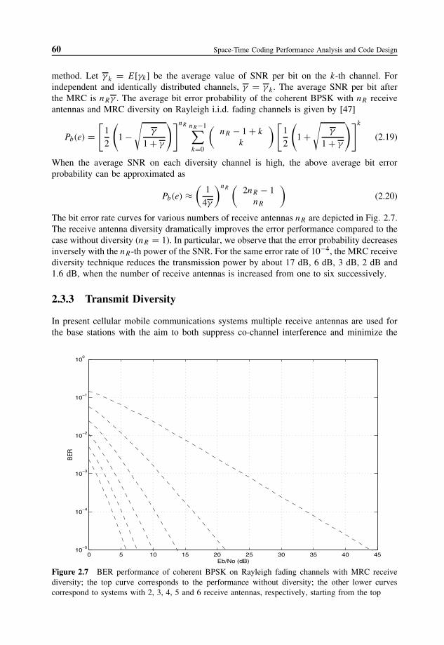
In Fig. 2.9, we plot the bit error rate performance of the scheme against Eb
N0for various
numbers of the transmit diversity nT . From this figure, we can observe that at the BER of10−4 the error performance is improved by about 14.5 dB, 4 dB and 2 dB, when the transmitdiversity order is increased from one to two, two to three and three to four, respectively.However, the performance curves suggest that a further increase in the transmit diversity canonly improve the performance by less than 1 dB. For a large number of diversity branches,the fading channel converges towards an AWGN channel, as the error performance curvefor a large nT almost approaches the one for the AWGN channel. It is important to mentionthat this feature plays an important role in deriving the space-time code design criteria,which are discussed later in this chapter.
In order to improve the error performance of the multiple antennas transmission, it is pos-sible to combine error control coding with the transmit diversity design. Various schemeshave been proposed to use error control coding in conjunction with multiple transmit anten-nas [22] [23]. Error control coding in combination with transmit diversity schemes canachieve a coding gain in addition to the diversity benefit, but suffers a loss in bandwidthdue to code redundancy.
A better alternative is a joint design of error control coding, modulation and transmitdiversity with no bandwidth expansion. This can be done by viewing coding, modulationand multiple transmission as one signal processing module. Coding techniques designed
Diversity 63
0 5 10 15 20 25 30 35 40 4510
−5
10−4
10−3
10−2
10−1
100
Eb/No (dB)
BER
Figure 2.9 BER performance of BPSK on Rayleigh fading channels with transmit diversity; the topcurve corresponds to the performance without diversity, and the bottom curve indicates the perfor-mance on AWGN channels; the curves in between correspond to systems with 2, 3, 4, 5, 6, 7, 8, 9,10, 15, 20 and 40 transmit antennas, respectively, starting from the top
for multiple antenna transmission are called space-time coding [6]. In particular, coding isperformed by adding properly designed redundancy in both spatial and temporal domains,which introduces correlation into the transmitted signals. Due to joint design, space-timecodes can achieve transmit diversity as well as a coding gain without sacrificing bandwidth.Space-time codes can be further combined with multiple receive antennas to minimize theeffects of multipath fading and to achieve the capacity of MIMO systems.
S/PInformation
source
Space-time
encoder
xnTt
x1t
x2t
ct xt
�
�
�
�
�
�
rnRt
r2t
r1t
Receiver �
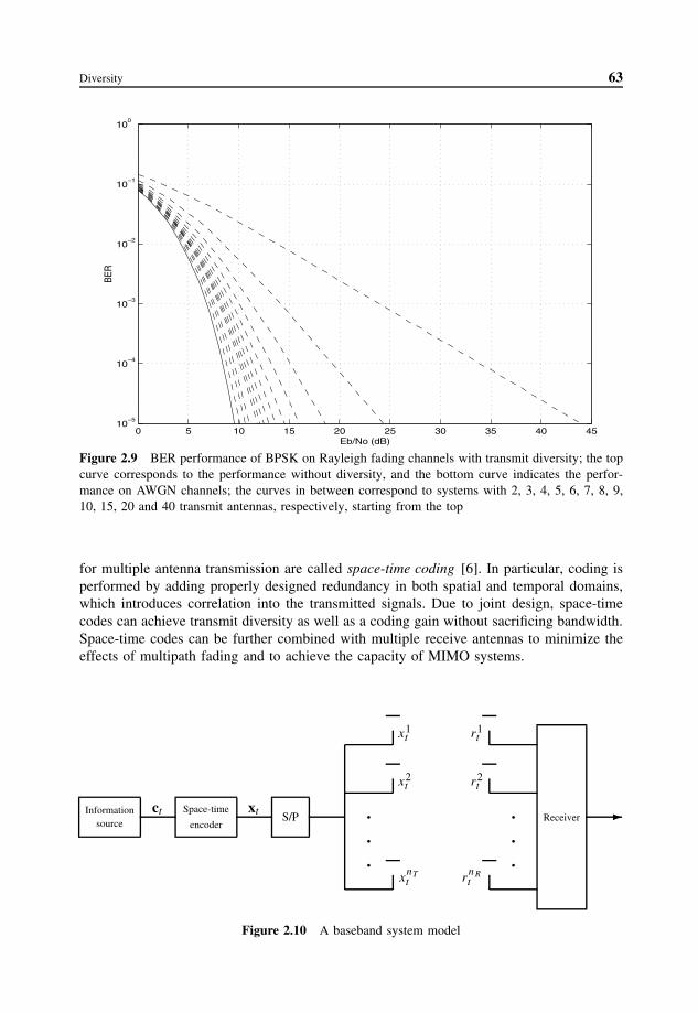
Figure 2.10 A baseband system model

64 Space-Time Coding Performance Analysis and Code Design
2.4 Space-Time Coded Systems
We consider a baseband space-time coded communication system with nT transmit antennasand nR receive antennas, as shown in Fig. 2.10. The transmitted data are encoded by aspace-time encoder. At each time instant t , a block of m binary information symbols,denoted by
ct = (c1t , c2
t , . . . , cmt ) (2.23)
is fed into the space-time encoder. The space-time encoder maps the block of m binaryinput data into nT modulation symbols from a signal set of M = 2m points. The codeddata are applied to a serial-to-parallel (S/P) converter producing a sequence of nT parallelsymbols, arranged into an nT × 1 column vector
xt = (x1t , x2
t , . . . , xnTt )T , (2.24)
where T means the transpose of a matrix. The nT parallel outputs are simultaneouslytransmitted by nT different antennas, whereby symbol xi
t , 1 ≤ i ≤ nT , is transmitted byantenna i and all transmitted symbols have the same duration of Tsec. The vector of codedmodulation symbols from different antennas, as shown in (2.24), is called a space-timesymbol. The spectral efficiency of the system is
η = rb
B= m bits/sec/Hz (2.25)
where rb is the data rate and B is the channel bandwidth. The spectral efficiency in (2.25)is equal to the spectral efficiency of a reference uncoded system with one transmit antenna.
The multiple antennas at both the transmitter and the receiver create a MIMO channel.For wireless mobile communications, each link from a transmit antenna to a receive
antenna can be modeled by flat fading, if we assume that the channel is memoryless. TheMIMO channel with nT transmit and nR receive antennas can be represented by an (nR×nT )channel matrix H. At time t , the channel matrix is given by
Ht =
ht1,1 ht
1,2 · · · ht1,nT
ht2,1 ht
2,2 · · · ht2,nT
......
. . ....
htnR,1 ht
nR,2 · · · htnR,nT
(2.26)
where the ji-th element, denoted by htj,i , is the fading attenuation coefficient for the path
from transmit antenna i to receive antenna j .In the analysis, we assume that the fading coefficients ht
j,i are independent complex
Gaussian random variables with mean µj,i
h and variance 1/2 per dimension, implying thatthe amplitude of the path coefficients are modeled as Rician fading. In terms of the coefficientvariation speed, we consider fast and slow fading channels. For slow fading, it is assumedthat the fading coefficients are constant during a frame and vary from one frame to another,which means that the symbol period is small compared to the channel coherence time. Theslow fading is also referred to as quasi-static fading [6]. In a fast fading channel, the fadingcoefficients are constant within each symbol period and vary from one symbol to another.

Performance Analysis of Space-Time Codes 65
At the receiver, the signal at each of the nR receive antennas is a noisy superpositionof the nT transmitted signals degraded by channel fading. At time t , the received signal atantenna j , j = 1, 2, . . . , nR , denoted by r
jt , is given by
rjt =
nT∑i=1
htj,ix
it + n
jt (2.27)
where njt is the noise component of receive antenna j at time t , which is an independent
sample of the zero-mean complex Gaussian random variable with the one sided powerspectral density of N0.
Let us represent the received signals from nR receive antennas at time t by an nR × 1column vector.
rt = (r1t , r2
t , . . . , rnRt )T (2.28)
The noise at the receiver can be described by an nR × 1 column vector, denoted by nt
nt = (n1t , n2
t , . . . , nnRt )T (2.29)
where each component refers to a sample of the noise at a receive antenna. Thus, thereceived signal vector can be represented as
rt = Htxt + nt (2.30)
We assume that the decoder at the receiver uses a maximum likelihood algorithm to estimatethe transmitted information sequence and that the receiver has ideal channel state information(CSI) on the MIMO channel. On the other hand, the transmitter has no information aboutthe channel. At the receiver, the decision metric is computed based on the squared Euclideandistance between the hypothesized received sequence and the actual received sequence as
∑t
nR∑j=1
∣∣∣∣∣rjt −
nT∑i=1
htj,ix
it
∣∣∣∣∣2
(2.31)
The decoder selects a codeword with the minimum decision metric as the decoded sequence.
2.5 Performance Analysis of Space-Time Codes
In the performance analysis we assume that the transmitted data frame length is L symbolsfor each antenna. We define an nT × L space-time codeword matrix, obtained by arrangingthe transmitted sequence in an array, as
X = [x1, x2, . . . , xL] =
x11 x1
2 · · · x1L
x21 x2
2 · · · x2L
......
. . ....
xnT
1 xnT
2 · · · xnT
L
(2.32)
where the i-th row xi = [xi1, xi
2, . . . , xiL] is the data sequence transmitted from the i-th
transmit antenna, and the t-th column xt = [x1t , x2
t , . . . , xnTt ]T is the space-time symbol at
time t .

66 Space-Time Coding Performance Analysis and Code Design
The pairwise error probability P (X, X̂) is the probability that the decoder selects as itsestimate an erroneous sequence X̂ = (X̂1, X̂2, . . . , X̂L) when the transmitted sequence wasin fact X = (x1, x2, . . . , xL). In maximum likelihood decoding, this occurs if
L∑t=1
nR∑j=1
∣∣∣∣∣rjt −
nT∑i=1
htj,ix
it
∣∣∣∣∣2
≥L∑
t=1
nR∑j=1
∣∣∣∣∣rjt −
nT∑i=1
htj,i x̂
it
∣∣∣∣∣2
(2.33)
The above inequality is equivalent to
L∑t=1
nR∑j=1
2Re
{(n
jt )
∗nT∑i=1
htj,i (x̂
it − xi
t )
}≥
L∑t=1
nR∑j=1
∣∣∣∣∣nT∑i=1
htj,i (x̂
it − xi
t )
∣∣∣∣∣2
(2.34)
where Re{·} means the real part of a complex number.Assuming that ideal CSI is available at the receiver, for a given realization of the fading
variable matrix sequence H = (H1, H2, . . . , HL), the term on the right hand side of (2.34)is a constant equal to d2
h(X, X̂) and the term on the left hand side of (2.34) is a zero-mean Gaussian random variable. d2
h(X, X̂) is a modified Euclidean distance between thetwo space-time codeword matrices X and X̂, given by
d2h(X, X̂) = ‖H · (X̂ − X)‖2
=L∑
t=1
nR∑j=1
∣∣∣∣∣nT∑i=1
htj,i (x̂
it − xi
t )
∣∣∣∣∣2
(2.35)
The pairwise error probability conditioned on H is given by
P (X, X̂|H) = Q
(√Es
2N0d2h(X, X̂)
)(2.36)
where Es is the energy per symbol at each transmit antenna and Q(x) is the complementaryerror function defined by
Q(x) = 1√2π
∫ ∞
x
e−t2/2dt (2.37)
By using the inequality
Q(x) ≤ 1
2e−x2/2, x ≥ 0 (2.38)
the conditional pairwise error probability (2.36) can be upper bounded by
P (X, X̂|H) ≤ 1
2exp
(−d2
h(X, X̂)Es
4N0
)(2.39)
2.5.1 Error Probability on Slow Fading Channels
On slow fading channels, the fading coefficients within each frame are constant. So we canignore the superscript of the fading coefficients
h1j,i = h2
j,i = · · · = hLj,i = hj,i ; i = 1, 2, . . . , nT , j = 1, 2, . . . , nR (2.40)

Performance Analysis of Space-Time Codes 67
Let us define a codeword difference matrix B(X, X̂) as
B(X, X̂) = X − X̂
=
x11 − x̂1
1 x12 − x̂1
2 · · · x1L − x̂1
L
x21 − x̂2
1 x22 − x̂2
2 · · · x2L − x̂2
L
......
. . ....
xnT
1 − x̂nT
1 xnT
2 − x̂nT
2 · · · xnT
L − x̂nT
L
(2.41)
We can construct an nT × nT codeword distance matrix A(X, X̂), defined as
A(X, X̂) = B(X, X̂) · BH(X, X̂) (2.42)
where H denotes the Hermitian (transpose conjugate) of a matrix. It is clear that A(X, X̂)
is nonnegative definite Hermitian, as A(X, X̂) = AH (X, X̂) and the eigenvalues of A(X, X̂)
are nonnegative real numbers [53]. Therefore, there exist a unitary matrix V and a realdiagonal matrix such that
VA(X, X̂)VH = (2.43)
The rows of V, {v1, v2, . . . , vnT}, are the eigenvectors of A(X, X̂), forming a complete
orthonormal basis of an N -dimensional vector space. The diagonal elements of are theeigenvalues λi ≥ 0, i = 1, 2, . . . , nT , of A(X, X̂). The diagonal matrix can be repre-sented as
=
λ1 0 · · · 00 λ2 · · · 0...
.... . .
...
0 0 · · · λnT
(2.44)
For simplicity, we assume that λ1 ≥ λ2 ≥ · · · ≥ λnT≥ 0.
Next, let
hj = (hj,1, hj,2, . . . , hj,nT) (2.45)
Equation (2.35) can be rewritten as
d2h(X, X̂) =
nR∑j=1
hj A(X, X̂)hjH
=nR∑j=1
nT∑i=1
λi |βj,i |2 (2.46)
where
βj,i = hj · vi (2.47)

68 Space-Time Coding Performance Analysis and Code Design
and · denotes the inner product of complex vectors. Substituting (2.46) into (2.39), we get
P (X, X̂|H) ≤ 1
2exp
−
nR∑j=1
nT∑i=1
λi |βj,i |2 Es
4N0
(2.48)
Inequality (2.48) is an upper bound on the conditional pairwise error probability expressedas a function of |βj,i |, which is contingent upon hj,i . Next, we determine the distributionof |βj,i | assuming the knowledge of hj,i .
Note that hj,i are complex Gaussian random variables with mean µj,ih and variance 1/2
per dimension and {v1, v2, . . . , vnT} is an orthonormal basis of an N -dimensional vector
space. It is obvious that βj,i in (2.47) are independent complex Gaussian random variableswith variance 1/2 per dimension and mean µ
j,iβ , where
µj,iβ = E[hj ] · E[vi]
= [µj,1h , µ
j,2h , . . . , µ
j,nT
h ] · vi (2.49)
where E[ · ] denotes the expectation. Let Kj,i = |µj,iβ |2, then |βj,i | has a Rician distribution
with the probability density function (pdf) [6]
p(|βj,i |) = 2|βj,i | exp(−|βj,i |2 − Kj,i)I0(2|βj,i |√
Kj,i) (2.50)
I0(·) is the zero-order modified Bessel function of the first kind.In order to get an upper bound on the unconditional pairwise error probability, we need
to average (2.48) with respect to the Rician random variables |βj,i |. Let r denote the rankof the matrix A(X, X̂). In this analysis, we distinguish two cases, depending on the valueof rnR .
The Pairwise Error Probability Upper Bound for Large Values of rnR
Since |βj,i | has a Rician distribution, |βj,i |2 has a noncentral chi-square distribution with 2degrees of freedom and noncentrality parameter S = |µj,i
β |2 = Kj,i . The mean value and
the variance of the noncentral chi-square-distributed random variables |βj,i |2 are given by
µ|βj,i |2 = 1 + Kj,i (2.51)
and
σ 2|βj,i |2 = 1 + 2Kj,i , (2.52)
respectively.At the right hand side of inequality (2.48), there are rnR independent chi-square-distri-
buted random variables. For a large value of rnR (rnR ≥ 4), which corresponds to alarge number of independent subchannels, according to the central limit theorem [54], theexpression
nR∑j=1
nT∑i=1
λi |βj,i |2 (2.53)

Performance Analysis of Space-Time Codes 69
approaches a Gaussian random variable D with the mean
µD =nR∑j=1
nT∑i=1
λi(1 + Kj,i) (2.54)
and the variance
σ 2D =
nR∑j=1
nT∑i=1
λ2i (1 + 2Kj,i) (2.55)
The pairwise error probability can then be upper-bounded by
P (X, X̂) ≤∫ +∞
D=0
1
2exp
(− Es
4N0D
)p(D)dD (2.56)
where p(D) is the pdf of the Gaussian random variable D. Using the equation
∫ +∞
D=0exp(−γD)p(D)dD = exp
(1
2γ 2σ 2
D − γµD
)Q
(γ σ 2
D − µD
σD
), γ > 0 (2.57)
the upper bound in (2.56) can be further expressed as
P (X, X̂) ≤ 1
2exp
(1
2
(Es
4N0
)2
σ 2D − Es
4N0µD
)Q
(Es
4N0σD − µD
σD
)(2.58)
Let us now consider the special case of Rayleigh fading. In this case, µj,ia = 0 and thus
Kj,i = 0. The mean and the variance of the Gaussian random variable D become
µD = nR
r∑i=1
λi (2.59)
and
σ 2D = nR
r∑i=1
λ2i , (2.60)
respectively. Substituting (2.59) and (2.60) into (2.58), we obtain the pairwise error proba-bility upper bound on Rayleigh fading channels as
P (X, X̂) ≤ 1
2exp
(1
2
(Es
4N0
)2
nR
r∑i=1
λ2i − Es
4N0nR
r∑i=1
λi
)
·Q
Es
4N0
√√√√nR
r∑i=1
λ2i −
√nR
∑ri=1 λi√∑r
i=1 λ2i
(2.61)

70 Space-Time Coding Performance Analysis and Code Design
The Pairwise Error Probability Upper Bound for Small Values of rnR
When the number of independent subchannels rnR is small, e.g. rnR < 4, the Gaussianassumption is no longer valid and the pairwise error probability can be expressed as
P (X, X̂) ≤∫
· · ·∫ ∞
|βj,i |=0P (X, X̂|H)p(|β1,1|)p(|β1,2|) · · ·p(|βnR,nT
|)
· d|β1,1|d|β1,2| · · · d|βnR,nT| (2.62)
where |βj,i | are independent Rician-distributed random variables with pdf in (2.50). Thisexpression can be integrated analytically term by term. By substituting (2.50) into (2.62),the pairwise error probability is upper bounded by [6]
P (X, X̂) ≤nR∏j=1
(nT∏i=1
1
1 + Es
4N0λi
exp
(−
Kj,i Es
4N0λi
1 + Es
4N0λi
))(2.63)
In the case of Rayleigh fading, the upper bound of the pairwise error probability becomes [6]
P (X, X̂) ≤(
nT∏i=1
1
1 + Es
4N0λi
)nR
(2.64)
At high SNR’s, the above upper bound can be simplified as [6]
P (X, X̂) ≤(
r∏i=1
λi
)−nR (Es
4N0
)−rnR
(2.65)
where r denotes the rank of matrix A(X, X̂), and λ1, λ2, . . . , λr are the nonzero eigenvaluesof matrix A(X, X̂).
Using a union bound technique, we can compute an upper bound of the code frame errorprobability, which sums the contributions of the pairwise error probabilities over all errorevents. Note that the pairwise error probability in (2.65) decreases exponentially with theincreasing SNR. The frame error probability at high SNR’s is dominated by the pairwiseerror probability with the minimum product rnR . The exponent of the SNR term, rnR , iscalled the diversity gain and
Gc = (λ1λ2 . . . λr)1/r
d2u
(2.66)
is called the coding gain, where d2u is the squared Euclidean distance of the reference
uncoded system. Note that both diversity and coding gains are obtained as the minimumrnR and (λ1λ2 . . . λr)
1/r over all pairs of distinct codewords. The diversity gain is anapproximate measure of the power gain of the system with space diversity over the systemwithout diversity at the same error probability. The coding gain measures the power gainof the coded system over an uncoded system with the same diversity gain, at the sameerror probability. The diversity gain determines the slope of an error rate curve plotted asa function of SNR, while the coding gain determines the horizontal shift of the uncodedsystem error rate curve to the space-time coded error rate curve obtained for the samediversity order.
Performance Analysis of Space-Time Codes 71
In general, to minimize the error probability, it is desirable to make both diversity andcoding gain as large as possible. Since the diversity gain is an exponent in the error proba-bility upper bound (2.65), it is clear that achieving a large diversity gain is more importantthan achieving a high coding gain for systems with a small value of rnR .
Example 2.2: A Time-Switched Space-Time Code
Let us consider a time-switched space-time code (TS STC)
X =[
xt 00 xt
](2.67)
where 0 means erasure. In this scheme, only one antenna is active in each time slot andthe modulated symbol xt is transmitted from antenna one and two at time 2t and 2t + 1,respectively. Since each modulated symbol is transmitted in two time slots, the code rate is1/2. Let
X̂ =[
x̂t 00 x̂t
](2.68)
be another codeword where xt = x̂t . The codeword difference matrix between the code-words is
B(X, X̂) =[
xt − x̂t 00 xt − x̂t
](2.69)
Since xt = x̂t , the rank of matrix B(X, X̂) is r = 2. Note that matrices A(X, X̂) and B(X, X̂)
have the same rank, as A(X, X̂) = B(X, X̂) · BH(X, X̂). This scheme achieves a diversitygain of two, if the number of receive antennas is one.
For a single receive antenna, the received signals at times 2t and 2t + 1, denoted by r1t
and r2t , respectively, are given by
r1t = h1
t xt + n1t
r2t = h2
t xt + n2t (2.70)
where h1t and h2
t are the channel fading coefficients between transmit antenna one and twoand the receive antenna, respectively, and n1
t and n2t are the noise samples at times 2t and
2t + 1, respectively. Let us assume that the fading coefficients are perfectly known at thereceiver. The maximum likelihood decoder chooses a signal x
′t from the modulation signal
set to minimize the squared Euclidean distance metric
d2(r1t , h1
t x′t ) + d2(r2
t , h2t x
′t ) (2.71)
Based on the MRC method, the receiver constructs a decision statistics signal, denoted byx̃t , as
x̃t = (h1t )
∗r1t + (h2
t )∗r2
t
=(|h1
t |2 + |h2t |2)
xt + (h1t )
∗n1t + (h2
t )∗n2
t (2.72)

72 Space-Time Coding Performance Analysis and Code Design
The maximum likelihood decoding rule can be rewritten as
x′t = arg min
(|h1
t |2 + |h2t |2 − 1
)+ d2(x̃t , x
′t ) (2.73)
The time-switched space-time code with a single receive antenna can achieve the samediversity gain of two as a two-branch MRC receive diversity scheme. However, the time-switched space-time code is of half rate and there is a 3 dB performance penalty relative tothe MRC receive diversity scheme.
Example 2.3: Repetition Code
We consider a space-time code by transmitting the same modulated symbols from twoantennas. The space-time codeword matrix is given by
X =[
xt
xt
](2.74)
The code rate is one. For any two distinct codewords with xt = x̂t , the codeword differencematrix is given by
B(X, X̂) =[
xt − x̂t
xt − x̂t
](2.75)
Obviously, the rank of the matrix is only one. Therefore, the repetition code has the sameperformance as a no diversity scheme (nT = nR = 1).
2.5.2 Error Probability on Fast Fading Channels
The analysis for slow fading channels in the previous section can be directly applied to fastfading channels.
At each time t , we define a space-time symbol difference vector F(xt , x̂t ) as
F(xt , x̂t ) = [x1t − x̂1
t , x2t − x̂2
t , . . . , xnTt − x̂
nTt ]T (2.76)
Let us consider an nT × nT matrix C(xt , x̂t ), defined as
C(xt , x̂t ) = F(xt , x̂t ) · FH (xt , x̂t ) (2.77)
It is clear that the matrix C(xt , x̂t ) is Hermitian. Therefore, there exist a unitary matrix Vt
and a real diagonal matrix Dt , such that
Vt · C(xt , x̂t ) · VHt = Dt (2.78)
The diagonal elements of Dt are the eigenvalues, Dit , i = 1, 2, . . . , nT , and the rows of Vt ,
{v1t , v2
t , . . . , vnTt }, are the eigenvectors of C(xt , x̂t ), forming a complete orthonormal basis
of an N -dimensional vector space.In the case that xt = x̂t , C(xt , x̂t ) is an all-zero matrix and all the eigenvalues Di
t ,i = 1, 2, . . . , nT , are zero. On the other hand, if xt = x̂t , the matrix C(xt , x̂t ) has onlyone nonzero eigenvalue and the other nT − 1 eigenvalues are zero. Let D1
t be the nonzero

Performance Analysis of Space-Time Codes 73
eigenvalue element which is equal to the squared Euclidean distance between the twospace-time symbols xt and x̂t .
D1t = |xt − x̂t |2 =
nT∑i=1
|xit − x̂i
t |2 (2.79)
The eigenvector of C(xt , x̂t ) corresponding to the nonzero eigenvalue D1t is denoted by v1
t .Let us define hj
t as
hjt = (ht
j,1, htj,2, . . . , ht
j,nT) (2.80)
Equation (2.35) can be rewritten as
d2h(X, X̂) =
L∑t=1
nR∑j=1
nT∑i=1
|βtj,i |2 · Di
t (2.81)
where
βtj,i = hj
t · vit (2.82)
Since at each time t there is at most only one nonzero eigenvalue, D1t , the expression (2.81)
can be represented by
d2h(X, X̂) =
∑t∈ρ(x,x̂)
nR∑j=1
|βtj,1|2 · D1
t
=∑
t∈ρ(x,x̂)
nR∑j=1
|βtj,1|2 · |xt − X̂t |2 (2.83)
where ρ(x, x̂) denotes the set of time instances t = 1, 2, . . . , L, such that |xt − x̂t | = 0.Substituting (2.83) into (2.39), we get
P (X, X̂|H) ≤ 1
2exp
−
∑t∈ρ(x, ˆ̂x)
nR∑j=1
|βtj,1|2|xt − x̂t |2 Es
4N0
(2.84)
Comparing (2.82) with (2.47), it is obvious that βtj,1 are also independent complex Gaussian
random variables with variance 1/2 per dimension and |βtj,1| follows a Rician distribution
with the pdf
p(|βtj,1|) = 2|βt
j,1| exp(−|βt
j,1|2 − Kj,1t
)I0
(2|βt
j,1|√
Kj,1t
)(2.85)
where
Kj,1t =
∣∣∣[µj,1ht
, µj,2ht
, . . . , µj,nT
ht] · v1
t
∣∣∣2 (2.86)
The conditional pairwise error probability upper bound (2.84) can be averaged over inde-pendent Rician-distributed variables |βt
j,1|. If we define δH as the number of space-time
symbols in which the two codewords X and X̂ differ, then at the right hand side of inequal-ity (2.84), there are δH nR independent random variables. As before, we will distinguishtwo cases in the analysis, depending on the value of δH nR . The term δH is also called thespace-time symbol-wise Hamming distance between the two codewords.

74 Space-Time Coding Performance Analysis and Code Design
The Pairwise Error Probability Upper Bound for Large δH nR
Provided that the value of δH nR for a given code is large, e.g., δH nR ≥ 4, according to thecentral limit theorem, the expression d2
h(X, X̂) in (2.83) can be approximated by a Gaussianrandom variable with the mean
µd =∑
t∈ρ(x,x̂)
nR∑j=1
|xt − x̂t |2(1 + Kj,1t ) (2.87)
and the variance
σ 2d =
∑t∈ρ(x,x̂)
nR∑j=1
|xt − x̂t |4(1 + 2Kj,1t ) (2.88)
By averaging (2.84) over the Gaussian random variable and using Eq. (2.57), the pairwiseerror probability can be upper-bounded by
P (X, X̂) ≤ 1
2exp
(1
2
(Es
4N0
)2
σ 2d − Es
4N0µd
)Q
(Es
4N0σd − µd
σd
)(2.89)
For Rayleigh fading channels, the pairwise error probability upper bound can be approxi-mated by
P (X, X̂) ≤ 1
2exp
(1
2
(Es
4N0
)2
nRD4 − Es
4N0nRd2
E
)Q
(Es
4N0
√nRD4 −
√nRd2
E√D4
)
(2.90)
where d2E is the accumulated squared Euclidean distance between the two space-time symbol
sequences, given by
d2E =
∑t∈ρ(x,x̂)
|xt − x̂t |2 (2.91)
and D4 is defined as
D4 =∑
t∈ρ(x,x̂)
|xt − x̂t |4 (2.92)
The Pairwise Error Probability Upper Bound for Small δH nR
When the value of δH nR is small, e.g., δH nR < 4, the central limit theorem argument isnot valid and the average pairwise error probability can be expressed as
P (X, X̂) ≤∫
· · ·∫ ∞
|βtj,1|=0
P (X, X̂|H)p(|β11,1|)p(|β1
2,1|) . . . p(|βLnR,1|)
· d|β11,1|d|β1
2,1| · · · d|βLnR,1| (2.93)

Space-Time Code Design Criteria 75
where |βtj,1|, t = 1, 2, . . . , L, and j = 1, 2, . . . , nR , are independent Rician-distributed
random variables with the pdf given by (2.85). By integrating (2.93) term by term, thepairwise error probability becomes [6]
P (X, X̂) ≤∏
t∈ρ(x,x̂)
nR∏j=1
1
1 + Es
4N0|xt − x̂t |2
exp
−
Kj,1t
Es
4N0|xt − x̂t |2
1 + Es
4N0|xt − x̂t |2
(2.94)
For a special case where |βtj,1| are Rayleigh distributed, the upper bound of the pairwise
error probability at high SNR’s becomes [6]
P (X, X̂) ≤∏
t∈ρ(x,x̂)
(1
1 + |xt − x̂t |2 Es
4N0
)nR
≤(d2p
)−nR(
Es
4N0
)−δH nR
(2.95)
where d2p is the product of the squared Euclidean distances between the two space-time
symbol sequences, given by
d2p =
∏t∈ρ(x,x̂)
|xt − x̂t |2 (2.96)
By using a union bound technique, we can compute an upper bound of the code frameerror probability, which sums the contributions of the pairwise error probabilities over allerror events. As the pairwise error probability in (2.95) decreases exponentially with theincreasing SNR, the frame error probability at high SNR’s is dominated by the pairwiseerror probability with the minimum product δH nR . The exponent of the SNR term, δH nR ,is called the diversity gain for fast Rayleigh fading channels and
Gc = (d2p)1/δH
d2u
(2.97)
is called the coding gain for fast Rayleigh fading channels, where d2u is the squared Euclidean
distance of the reference uncoded system. Note that both diversity and coding gains areobtained as the minimum δH nR and (d2
p)1/δH over all pairs of distinct codewords.
2.6 Space-Time Code Design Criteria
2.6.1 Code Design Criteria for Slow Rayleigh Fading Channels
As the error performance upper bounds (2.61) and (2.65) indicate, the design criteria forslow Rayleigh fading channels depend on the value of rnR . The maximum possible value ofrnR is nT nR . For small values of nT nR , corresponding to a small number of independentsubchannels, the error probability at high SNR’s is dominated by the minimum rank r
of matrix A(X, X̂) over all possible codeword pairs. The product of the minimum rankand the number of receive antennas, rnR , is called the minimum diversity. In addition,in order to minimize the error probability, the minimum product of nonzero eigenvalues,

76 Space-Time Coding Performance Analysis and Code Design
∏ri=1 λi , of matrix A(X, X̂) along the pairs of codewords with the minimum rank should
be maximized. Therefore, if the value of nT nR is small, the space-time code design criteriafor slow Rayleigh fading channels can be summarized as [6]:
Design Criteria Set I
[I-a] Maximize the minimum rank r of matrix A(X, X̂) over all pairs of distinct codewords
[I-b] Maximize the minimum product,∏r
i=1 λi , of matrix A(X, X̂) along the pairs ofdistinct codewords with the minimum rank
Note that∏r
i=1 λi is the absolute value of the sum of determinants of all the principalr × r cofactors of matrix A(X, X̂) [6]. This criteria set is referred to as rank & determinantcriteria. It is also called Tarokh/Seshadri/Calderbank (TSC) criteria. The minimum rankof matrix A(X, X̂) over all pairs of distinct codewords is called the minimum rank of thespace-time code.
To maximize the minimum rank r means to find a space-time code with the full rank ofmatrix A(X, X̂), e.g., r = nT . However, the full rank is not always achievable due to therestriction of the code structure. We discuss in detail how to design optimum space-timecodes in Chapters 3 and 4.
For large values of nT nR , corresponding to a large number of independent subchannels,the pairwise error probability is upper-bounded by (2.61). In order to get an insight into thecode design for systems of practical interest, we assume that the space-time code operatesat a reasonably high SNR, which can be represented as1
Es
4N0≥∑r
i=1 λi∑ri=1 λ2
i
(2.98)
By using the inequality
Q(x) ≤ 1
2e−x2/2, x ≥ 0 (2.99)
the bound in (2.61) can be further approximated as
P (X, X̂) ≤ 1
4exp
(−nR
Es
4N0
r∑i=1
λi
)(2.100)
The bound in (2.100) shows that the error probability is dominated by the codewords with theminimum sum of the eigenvalues of A(X, X̂). In order to minimize the error probability,the minimum sum of all eigenvalues of matrix A(X, X̂) among all the pairs of distinctcodewords should be maximized. For a square matrix the sum of all the eigenvalues isequal to the sum of all the elements on the matrix main diagonal, which is called the traceof the matrix [53]. It can be expressed as
tr(A(X, X̂)) =r∑
i=1
λi =nT∑i=1
Ai,i (2.101)
1The value of∑r
i=1 λi∑ri=1 λ2
i
is usually small. For example, its value for the 4-state QPSK space-time code in [6],
[25] and [30] is 0.5, 0.19 and 0.11, respectively.
Space-Time Code Design Criteria 77
where Ai,i are the elements on the main diagonal of matrix A(X, X̂). Since
Ai,j =L∑
t=1
(xit − x̂i
t )(xjt − x̂
jt )∗ (2.102)
substituting (2.102) into (2.101), we get
tr(A(X, X̂)) =nT∑i=1
L∑t=1
|xit − x̂i
t |2 (2.103)
Equation (2.103) indicates that the trace of matrix A(X, X̂) is equivalent to the squaredEuclidean distance between the codewords X and X̂. Therefore, maximizing the minimumsum of all eigenvalues of matrix A(X, X̂) among the pairs of distinct codewords, or theminimum trace of matrix A(X, X̂), is equivalent to maximizing the minimum Euclideandistance between all pairs of distinct codewords. This design criterion is called the tracecriterion.
It should be pointed out that formula (2.100) is valid for a large number of independentsubchannels under the condition that the minimum value of rnR is high. In this case, thespace-time code design criteria for slow fading channels can be summarized as
Design Criteria Set II
[II-a] Make sure that the minimum rank r of matrix A(X, X̂) over all pairs of distinctcodewords is such that rnR ≥ 4
[II-b] Maximize the minimum trace∑r
i=1 λi of matrix A(X, X̂) among all pairs of distinctcodewords
It is important to note that the proposed design criteria are consistent with those for trelliscodes over fading channels with a large number of diversity branches [38] [37]. A largenumber of diversity branches reduces the effect of fading and consequently, the channelapproaches an AWGN model. Therefore, the trellis code design criteria derived for AWGNchannels [36], which is maximizing the minimum code Euclidean distance, apply to fadingchannels with a large number of diversity. In a similar way, in space-time code design,when the number of independent subchannels rnR is large, the channel converges to anAWGN channel. Thus, the code design is the same as that for AWGN channels.
From the above discussion, we can conclude that either the rank & determinant criteriaor the trace criterion should be applied for design of space-time codes, depending on thediversity order rnR . When rnR < 4, the rank & determinant criteria should be applied andwhen rnR ≥ 4, the trace criterion should be applied.
The boundary value of rnR between the two design criteria sets was chosen to be 4.This boundary is determined by the required number of random variables rnR in (2.53) tosatisfy the central limit theorem. In general, for random variables with smooth pdf’s, thecentral limit theorem can be applied if the number of random variables in the sum is largerthan 4 [54]. In the application of the central limit theorem in (2.53), the choice of 4 as theboundary has been further justified by the code design and performance simulation, as itwas found that as long as rnR ≥ 4, the best codes based on the trace criterion outperformthe best codes based on the rank and determinant criteria [31] [34].

78 Space-Time Coding Performance Analysis and Code Design
2.6.2 Code Design Criteria for Fast Rayleigh Fading Channels
As the error performance upper bounds (2.90) and (2.95) indicate, the code design criteriafor fast Rayleigh fading channels depend on the value of δH nR . For small values of δH nR ,the error probability at high SNR’s is dominated by the minimum space-time symbol-wiseHamming distance δH over all distinct codeword pairs. In addition, in order to minimizethe error probability, the minimum product distance, d2
p, along the path of the pairs ofcodewords with the minimum symbol-wise Hamming distance δH , should be maximized.Therefore, if the value of δH nR is small, the space-time code design criteria for fast fadingchannels can be summarized as [6]:
Design Criteria Set III
[III-a] Maximize the minimum space-time symbol-wise Hamming distance δH between allpairs of distinct codewords
[III-b] Maximize the minimum product distance, d2p, along the path with the minimum
symbol-wise Hamming distance δH
For large values of δH nR the pairwise error probability is upper-bounded by (2.90). Asbefore, we assume the space-time code works at a reasonably high SNR, which corre-sponds to
Es
4N0≥ d2
E
D4(2.104)
where d2E and D4 are given by (2.91) and (2.92), respectively. By using the inequality
(2.99), the bound (2.90) can be further approximated by
P (X, X̂) ≤ exp
(−nR
Es
4N0
L∑t=1
nT∑i=1
|xit − x̂i
t |2)
= exp
(−nR
Es
4N0d2E
)(2.105)
From (2.105), it is clear that the frame error probability at high SNR’s is dominated by thepairwise error probability with the minimum squared Euclidean distance d2
E . To minimizethe error probability on fading channels, the codes should satisfy
Design Criteria Set IV
[IV-a] Make sure that the product of the minimum space-time symbol-wise Hamming dis-tance and the number of receive antennas, δH nR , is large enough (larger than orequal to 4)
[IV-b] Maximize the minimum Euclidean distance among all pairs of distinct codewords.
It is interesting to note that this design criterion is the same as the trace criterion for space-time code on slow fading channels if the value of rnR is large. It is also consistent withthe design criterion for trellis coded modulation on fading channels if the symbol-wiseHamming distance is large [38].

Space-Time Code Design Criteria 79
Based on the previous discussion, we can conclude that code design on fading channelsis very much dependent on the possible diversity order of the space-time coded system. Forcodes on slow fading channels, the total diversity is the product of the receive diversity, nR ,and the transmit diversity provided by the code scheme, r . On the other hand, for codes onfast fading channels, the total diversity is the product of the receive diversity, nR , and thetime diversity achieved by the code scheme, δH . If the total diversity is small, in the codedesign for slow fading channels one should attempt to maximize the diversity and the codinggain by choosing a code with the largest minimum rank and the determinant; while for fastfading channels one should attempt to choose a code with the largest minimum symbol-wiseHamming distance and the product distance. In this case, the diversity gain dominates thecode performance and it has much more influence on error probability than the coding gain.However, when the total diversity is getting larger, increasing the diversity order cannotachieve a substantial performance improvement. In contrast, the coding gain becomes moreimportant. Since a high order of diversity drives the fading channel towards an AWGNchannel as shown in Fig. 2.9, the error probability is dominated by the minimum Euclideandistance. Thus, the code design criterion for AWGN channels, which is maximizing theminimum Euclidean distance, is valid for both slow and fast fading channels provided thatthe diversity is large.
Example 2.4
To illustrate the design criteria and evaluate the importance of the rank, determinant andtrace in determining the code performance for systems with various numbers of the transmitand receive antennas on slow Rayleigh fading channels, we consider the following example.
Let us consider three QPSK space-time trellis codes with 4 states and 2 transmit antennas.The three codes are denoted by A, B and C, respectively. The code trellis structures areshown in Fig. 2.11. These codes have the same bandwidth efficiency of 2 bits/s/Hz. Theminimum rank, determinant and trace of the codes are also listed in Fig. 2.11. It is shownthat codes A and B have a full rank and the same determinant of 4, while code C is notof full rank and therefore, its determinant is 0. On the other hand, the minimum trace forcodes B and C is 10 while code A has a smaller minimum trace of 4.
�
�
�
�
�
�
�
�
������
��������
�����������
������
������
��������
��������
������
�������
����������
��������
������
00 01 02 03
10 11 12 13
20 21 22 23
30 31 32 33
rank:2 det:4 trace:4
code A
�
�
�
�
�
�
�
�
������
��������
�����������
������
������
��������
��������
������
�������
����������
��������
������
00 23 02 21
20 03 22 01
12 31 10 33
32 11 30 13
rank:2 det:4 trace:10
code B
�
�
�
�
�
�
�
�
������
��������
�����������
������
������
��������
��������
������
�������
����������
��������
������
00 23 02 21
02 21 00 23
22 01 20 03
20 03 22 01
rank:1 det:0 trace:10
code C
Figure 2.11 Trellis structures for 4-state space-time coded QPSK with 2 antennas

80 Space-Time Coding Performance Analysis and Code Design
0 5 10 15 20 25 30 3510
3
102
101
100
SNR (dB)
Fram
e Er
ror P
roba
bilit
y
Code ACode BCode Cn
R=1
nR=4
Figure 2.12 FER performance of the 4-state space-time trellis coded QPSK with 2 transmit antennas,Solid: 1 receive antenna, Dash: 4 receive antennas
The performance of the codes with various numbers of the receive antennas on slowRayleigh fading channels is evaluated by simulation. The frame length was 130 symbols.The frame error rate (FER) performance versus the SNR per receive antenna, e.g., SNR =nT Es/N0, is shown in Fig. 2.12.
From Fig. 2.12, it can be observed that codes A and B outperform code C if one receiveantenna is employed. This is explained as follows. When the number of independent sub-channels nT nR is small, the minimum rank of the code dominates the code performance.Since both code A and code B are of full rank (r = 2) and code C is not (r = 1), codes Aand B achieve a better performance relative to code C. It can also be seen that the perfor-mance curves for codes A and B have an asymptotic slope of −2 while the slope for codeC is −1, consistent with the diversity order of 2 for codes A and B, and 1 for code C. Ata FER of 10−2, codes A and B outperform code C by about 5 dB due to a larger diversityorder. It clearly indicates that the minimum rank is much more important in determiningthe code performance for systems with a small number of independent subchannels.
However, when the number of receive antennas is 4, code C performs better than code Aas shown in Fig. 2.12, which means the code with a full rank is worse than the code witha smaller rank. This occurs as the diversity gain rnR in this case is 8 and 4 for codes Aand C, respectively. According to Design Criteria II, code C is superior to code A due toa larger minimum trace value. At a FER of 10−2, the advantage of the code C relative tocode A is about 1.3 dB.
From Fig. 2.12 we can also see that code B is about 0.8 dB better than code C at theFER of 10−2, although they have the same minimum trace. This is due to the fact thatcode B has the same minimum trace and a larger rank than code C. Therefore, code B canachieve a larger diversity, which is manifested by a steeper error rate slope for code B thanfor code C.

Space-Time Code Design Criteria 81
When the number of receive antennas increases further to 6, it is shown in [31] that theperformance of code B on slow Rayleigh fading channels is very close to its performanceon AWGN channels, which verifies the convergence of Rayleigh fading channels to AWGNchannels, provided a large diversity is available.
This example clearly verified the code design criteria for slow fading channels.
2.6.3 Code Performance at Low to Medium SNR Ranges
The code design criteria are derived based on the asymptotic code performance at very highSNR’s. However, in practical communication systems, given the number of transmit andreceive antennas to be used and the FER performance requirement, the code may work ata low or a medium SNR range. Let us denote Es
4N0by γ . We assume that γ � 1 refers
to a high SNR range, γ 1 as a low SNR range and γ ≈ 1 as a medium SNR range.For example, for two transmit and two receive antennas, to achieve the FER of 10−2 andbandwidth efficiency of 2 bits/s/Hz, the space-time coded QPSK will work around the SNRof about 10 dB. This SNR corresponds to γ ≈ 1, so the previous code design criteriaderived for very high SNR’s may not be very accurate.
In [29], modified design criteria for space-time codes under various SNR conditions arediscussed. Recall the pairwise error probability upper bound in (2.64). The bound can berewritten as
P (X, X̂) ≤(
nT∏i=1
1
1 + γ λi
)nR
(2.106)
We will consider three different cases.
CASE 1: γ 1
This case refers to a low SNR range. Since γ 1, when the denominator in the upperbound (2.106) is expanded, one can ignore the contribution of the high order terms of γ ,so that the upper bound becomes
P (X, X̂) ≤(
1 + γ
r∑i=1
λi
)−nR
(2.107)
Recall that the sum of the eigenvalues is equal to the trace. From this bound, we can seethat in the code design for a low SNR range, the minimum trace should be maximized.This means that in order to achieve a specified FER at a low SNR, nT and/or nR need tobe large. In other words, this case falls into the situation of large values of nT nR as wediscussed previously.
CASE 2: γ � 1
This case refers to a very high SNR range. Under this condition, the space-time codeperformance is upper bounded by [6]
P (X, X̂) ≤(
r∏i=1
λi
)−nR
γ −rnR (2.108)
82 Space-Time Coding Performance Analysis and Code Design
It is obvious that the rank & determinant criteria should be used in code design. For aspecified FER, if nT nR is small, the SNR is typically large (γ � 1). Therefore, this casefalls into the domain of small values of nT nR as we discussed previously.
CASE 3: γ ≈ 1
The case refers to a moderate SNR range. As we predicted by analysis and confirmedby simulation, the typical SNR for a space-time code with two transmit and two receiveantennas to achieve the FER of 10−2 and bandwidth efficiency of 2 bits/s/Hz is around10 dB. For this SNR value, γ = Es
4N0= SNR
4nT= 10
8 ≈ 1. In this range, for γ ≈ 1, thepairwise upper bound becomes
P (X, X̂) ≤(
nT∏i=1
1
1 + λi
)nR
(2.109)
We can formulate the code design criterion as maximizing the minimum determinant of thematrix I + A(X, X̂), where I is an nT × nT identical matrix. This criterion is derived for avery specific SNR. In practical systems, space-time codes may work at a range of SNR’s.Good codes designed by this criterion may not be optimal in the whole range of SNR’s.Therefore, this criterion is less practical relative to other design criteria.
2.7 Exact Evaluation of Code Performance
In the previous code performance analysis and code design, we considered only the worstcase pairwise error probability upper bound. In order to get the accurate performance eval-uation, one possible method is to compute the code distance spectrum and apply the unionbound technique to calculate the average pairwise error probability. The obtained upperbound is asymptotically tight at high SNR’s for a small number of receive antennas butloose for other scenarios [41]. A more accurate performance evaluation can be obtainedwith exact evaluation of the pairwise error probability, rather than evaluating the bounds.This can be done by using residue methods based on the characteristic function technique[42] [43] or on the moment generating function method [44] [45].
Recall that the pairwise error probability conditioned on the MIMO fading coefficients isgiven by
P (X, X̂|H) = Q
√√√√ Es
2N0
L∑t=1
‖Ht (xt − x̂t )‖2
(2.110)
Let
� = Es
2N0
L∑t=1
‖Ht (xt − x̂t )‖2 (2.111)
By using Graig’s formula for the Gaussian Q function [48]
Q(x) = 1
π
∫ π/2
0exp
(− x2
2 sin2 θ
)dθ (2.112)

Exact Evaluation of Code Performance 83
we can rewrite for the conditional pairwise error probability
P (X, X̂|H) = 1
π
∫ π/2
0exp
(− �2
2 sin2 θ
)dθ (2.113)
In order to compute the average pairwise error probability, we average (2.113) with respectto the distribution of �. The average pairwise error probability can be expressed in termsof the moment generating function (MGF) of �, denoted by M�(s), which is given by
M�(s) =∫ ∞
0es�P�(�) d� (2.114)
The average pairwise error probability can be represented as [44]
P (X, X̂) = 1
π
∫ π/2
0E
[exp
(− �2
2 sin2 θ
)]dθ
= 1
π
∫ π/2
0
∫ ∞
0exp
(− �2
2 sin2 θ
)P�(�)d� dθ
= 1
π
∫ π/2
0M�
(− 1
2 sin2 θ
)dθ (2.115)
For fast Rayleigh fading MIMO channels, the MGF can be expressed in a closed formas [44]
M�(s) =L∏
t=1
[1 − sEs
2N0
nT∑i=1
|xit − x̂i
t |2]−nR
(2.116)
where
s = − 1
2 sin2 θ. (2.117)
Substituting (2.116) into (2.115), we get for the average pairwise error probability
P (X, X̂) = 1
π
∫ π/2
0
L∏t=1
[1 + Es
4N0 sin2 θ
nT∑i=1
|xit − x̂i
t |2]−nR
dθ (2.118)
For slow Rayleigh fading channels, the MGF can be represented as [44]
M�(s) =(
det
[InT
− s(X − X̂)(X − X̂)HEs
2N0
])−nR
. (2.119)
If the rows of matrix (X − X̂) are orthogonal, this MGF can be simplified as
M�(s) =nT∏i=1
[1 − sEs
2N0
L∑t=1
|xit − x̂i
t |2]−nR
. (2.120)
In this case, the average pairwise error probability is given by
P (X, X̂) = 1
π
∫ π/2
0
nT∏i=1
[1 + Es
4N0 sin2 θ
L∑t=1
|xit − x̂i
t |2]−nR
dθ. (2.121)
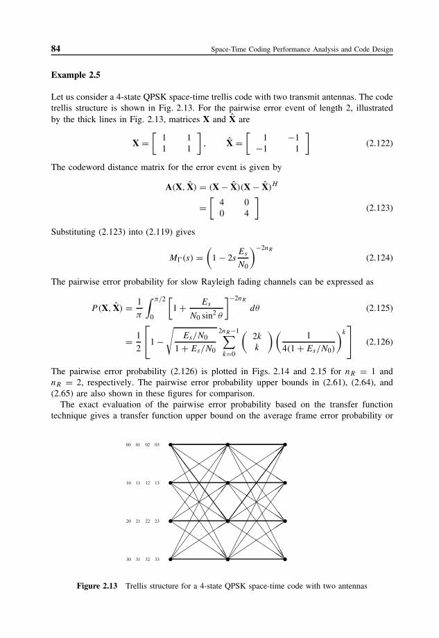
84 Space-Time Coding Performance Analysis and Code Design
Example 2.5
Let us consider a 4-state QPSK space-time trellis code with two transmit antennas. The codetrellis structure is shown in Fig. 2.13. For the pairwise error event of length 2, illustratedby the thick lines in Fig. 2.13, matrices X and X̂ are
X =[
1 11 1
], X̂ =
[1 −1
−1 1
](2.122)
The codeword distance matrix for the error event is given by
A(X, X̂) = (X − X̂)(X − X̂)H
=[
4 00 4
](2.123)
Substituting (2.123) into (2.119) gives
M�(s) =(
1 − 2sEs
N0
)−2nR
(2.124)
The pairwise error probability for slow Rayleigh fading channels can be expressed as
P (X, X̂) = 1
π
∫ π/2
0
[1 + Es
N0 sin2 θ
]−2nR
dθ (2.125)
= 1
2
1 −
√Es/N0
1 + Es/N0
2nR−1∑k=0
(2k
k
)(1
4(1 + Es/N0)
)k
(2.126)
The pairwise error probability (2.126) is plotted in Figs. 2.14 and 2.15 for nR = 1 andnR = 2, respectively. The pairwise error probability upper bounds in (2.61), (2.64), and(2.65) are also shown in these figures for comparison.
The exact evaluation of the pairwise error probability based on the transfer functiontechnique gives a transfer function upper bound on the average frame error probability or
�
�
�
�
�
�
�
��������
���������
�������������
�������
�������
���������
���������
�������
��������
������������
���������
�������
00 01 02 03
10 11 12 13
20 21 22 23
30 31 32 33 �
�
�
�
�
�
�
��������
���������
�������������
�������
�������
���������
���������
�������
��������
������������
���������
�������
Figure 2.13 Trellis structure for a 4-state QPSK space-time code with two antennas

Exact Evaluation of Code Performance 85
−5 0 5 10 15 2010
−5
10−4
10−3
10−2
10−1
100
Es/No (dB)
Pairw
ise
Erro
r Pro
babi
lity
exact (2.126)bound (2.65)bound (2.64)bound (2.61)
Figure 2.14 Pairwise error probability of the 4-state QPSK space-time trellis code with two transmitand one receive antenna
−10 −8 −6 −4 −2 0 2 4 6 8 1010
−5
10−4
10−3
10−2
10−1
100
Es/No (dB)
Pairw
ise
Erro
r Pro
babi
lity
exact (2.126)bound (2.65)bound (2.64)bound (2.61)
Figure 2.15 Pairwise error probability of the 4-state QPSK space-time trellis code with two transmitand two receive antennas

86 Space-Time Coding Performance Analysis and Code Design
4 6 8 10 12 14 16 18 20 22 2410
−5
10−4
10−3
10−2
10−1
100
SNR (dB)
Bit e
rror R
ate
Upper boundSimulation
Simulation, 2Tx 2Rx
upper bound, 2Tx 2Rx
upper bound, 2Tx 1Rx
Simulation, 2Tx 1Rx
Figure 2.16 Average bit error rate of the 4-state QPSK space-time trellis code with two transmitantennas and one and two receive antennas
bit error probability for space-time codes, which is asymptotically tight at high SNR’s andtighter than a Chernoff bound [44].
Figure 2.16 illustrates the performance comparison between the analytical and simulatedaverage bit error rate of the 4-state QPSK space-time trellis code with two transmit antennasand one and two receive antennas on slow Rayleigh fading channels. In the analyticalevaluating the average bit error rate, only the error events of lengths two and three areconsidered for simplicity.
Bibliography
[1] G. J. Foschini and M. Gans, “On the limits of wireless communication in a fadingenvironment when using multiple antennas”, Wireless Personal Communication, vol. 6,pp. 311–335, Mar. 1998.
[2] G. J. Foschini, “Layered space-time architecture for wireless communication in fadingenvironments when using multiple antennas”, Bell Labs Tech. J., 2, Autumn 1996.
[3] E. Telatar, “Capacity of multi-antenna Gaussian channels”, Technical Report, AT&T-Bell Labs, June 1995, and ETT, vol. 10, no. 6, pp. 585–595, Nov. 1999.
[4] B. Hochwald and T. L. Marzetta, “Capacity of a mobile multiple-antenna communica-tion link in a Rayleigh flat fading environment”, IEEE Trans. Inform. Theory, vol. 45,no. 1, pp. 139–157, Jan. 1999.
[5] G. G. Raleigh and J.M. Cioffi, “Spatio-temporal coding for wireless communication”,IEEE Trans. Communi., vol. 46, no. 3, pp. 357–366, Mar. 1998.

Bibliography 87
[6] V. Tarokh, N. Seshadri and A. R. Calderbank, “Space-time codes for high data ratewireless communication: performance criterion and code construction”, IEEE Trans.Inform. Theory, vol. 44, no. 2, pp. 744–765, Mar. 1998.
[7] J.-C. Guey, M. R. Bell, M. P. Fitz and W. Y. Kuo, “Signal design for transmitterdiversity wireless communication systems over Rayleigh fading channels”, in Proc.IEEE Vehicular Technology Conference, pp. 136–140, Atlanta, US, 1996, and IEEETrans. Commun., vol. 47, no. 4, pp. 527–537, Apr. 1998.
[8] A. Naguib, V. Tarokh, N. Seshadri and A. Calderbank, “A space-time coding modemfor high-data-rate wireless communications”, IEEE J. Select. Areas Commun., vol. 16,no. 10, pp. 1459–1478, Oct. 1998.
[9] S. M. Alamouti, “A simple transmit diversity technique for wireless communications”,IEEE J. Select. Areas Commun., vol. 16, no. 10, pp. 1451–1458, Oct. 1998.
[10] V. Tarokh, H. Jafarkhani and A. R. Calderbank, “Space-time block codes from ortho-gonal designs”, IEEE Trans. Inform. Theory, vol. 45, no. 5, pp. 1456–1467, July1999.
[11] V. Tarokh, H. Jafarkhani and A. R. Calderbank, “Space-time block coding for wirelesscommunications: performance results”, IEEE J. Select. Areas Commun., vol. 17, no. 3,pp. 451–460, Mar. 1999.
[12] J. Grimm, M. P. Fitz and J. V. Krogmeier, “Further results in space-time coding forRayleigh fading”, in Proc. 36th Allerton Conference on Communications, Control andComputing, Sep. 1998.
[13] V. Tarokh, A. Naguib, N. Seshadri and A. R. Calderbank, “Combined array processingand space-time coding”, IEEE Trans. Inform. Theory, vol. 45, no. 4, pp. 1121–1128,May 1999.
[14] V. Tarokh, A. Naguib, N. Seshadri and A. R. Calderbank, “Space-time codes for highdata rate wireless communication: performance criteria in the presence of channelestimation errors, mobility, and multiple paths”, IEEE Trans. Commun., vol. 47, no. 2,pp. 199–207, Feb. 1999.
[15] A. F. Naguib and R. Calderbank, “Space-time coding and signal processing for highdata rate wireless communications”, IEEE Signal Processing Magazine, vol. 17, no. 3,pp. 76–92, Mar. 2000.
[16] J. H. Winters, “Switched diversity with feedback for DPSK mobile radio systems”,IEEE Trans. Vehicular Technology, vol. 32, pp. 134–150, 1983.
[17] A. Wittneben, “Base station modulation diversity for digital SIMULCAST”, in Proc.IEEE Vehicular Technology Conf., vol. 1, pp. 848–853, May 1991.
[18] A. Winttneben, “A new bandwidth efficient transmit antenna modulation diversityscheme for linear digital modulation”, in Proc. 1993 IEEE International Conf. Com-munications (ICC93), pp. 1630–1634, May 1993.
[19] N. Seshadri and J. H. Winters, “Two signaling schemes for improving the error per-formance of FDD transmission systems using transmitter antenna diversity”, in Proc.1993 IEEE Vehicular Technology Conf., pp. 508–511, May 1993.
[20] J. H. Winters, “The diversity gain of transmit diversity in wireless systems withRayleigh fading”, in Proc. 1994 IEEE International Conf. Communications (ICC94),vol. 2, pp. 1121–1125, New Orleans, LA, May 1994.
[21] J. H. Winters, “The diversity gain of transmit diversity in wireless systems withRayleigh fading”, IEEE Trans. Vehicular Technology, vol. 47, pp. 119–123, 1998.

88 Space-Time Coding Performance Analysis and Code Design
[22] A. Hiroike, F. Adachi and N. Nakajima, “Combined effects of phase sweeping transmit-ter diversity and channel coding”, IEEE Trans. Vehicular Technology, vol. 42, pp. 170–176, 1992.
[23] A. Hiroike and K. Hirade, “Multitransmitter simulcast digital signal transmission byusing frequency offset strategy in land mobile radio telephone”, IEEE Trans. VehicularTechnology, vol. 27, pp. 231–238, 1978.
[24] A. R. Hammons and H. E. Gammal, “On the theory of space-time codes for PSKmodulation”, IEEE Trans. on. Inform. Theory, vol. 46, no. 2, pp. 524–542, Mar. 2000.
[25] S. Baro, G. Bauch and A. Hansmann, “Improved codes for space-time trellis codedmodulation”, IEEE Commun. Lett., vol. 4, no. 1, pp. 20–22, Jan. 2000.
[26] R. S. Blum, “New analytical tools for designing space-time convolutional codes”,Invited paper at CISS, Princeton University, Princeton, NJ, Mar. 2000, also submittedto IEEE Trans. on Inform. Theory.
[27] Q. Yan and R. S. Blum, “Optimum space-time convolutional codes”, in Proc. IEEEWCNC’00, Chicago, IL., pp. 1351–1355, Sep. 2000.
[28] D. M. Ionescu, K. K. Mukkavilli, Z. Yan and J. Lilleberg, “Improved 8- and 16-statespace-time codes for 4PSK with two transmit antennas”, IEEE Commun. Lett., vol. 5,pp. 301–303, Jul. 2001.
[29] M. Tao and R. S. Cheng, “Improved design criteria and new trellis codes for space-timecoded modulation in slow flat fading channels”, IEEE Comm. Lett., vol. 5, pp. 313–315, Jul. 2001.
[30] Z. Chen, J. Yuan and B. Vucetic, “Improved space-time trellis coded modulationscheme on slow Rayleigh fading channels”, Electron. Lett., vol. 37, no. 7, pp. 440–441,Mar. 2001.
[31] Z. Chen, J. Yuan and B. Vucetic, “An improved space-time trellis coded modulationscheme on slow Rayleigh fading channels”, in Proc. IEEE ICC’01, Helsinki, Finland,pp. 1110–1116, Jun. 2001.
[32] J. Yuan, B. Vucetic, B. Xu and Z. Chen, “Design of space-time codes and its perfor-mance in CDMA systems”, in Proc. IEEE Vehicular Technology Conf., pp. 1292–1296,May 2001.
[33] J. Yuan, Z. Chen, B. Vucetic and W. Firmanto, “Performance analysis of space-timecoding on fading channels”, in Proc. IEEE ISIT’01, Washington D.C., pp. 153, Jun.2001.
[34] J. Yuan, Z. Chen, B. Vucetic and W. Firmanto, “Performance analysis and design ofspace-time coding on fading channels”, submitted to IEEE Trans. Commun..
[35] W. Firmanto, B. Vucetic and J. Yuan, “Space-time TCM with improved performanceon fast fading channels”, IEEE Commun. Lett., vol. 5, no. 4, pp. 154–156, Apr. 2001.
[36] G. Ungerboeck, “Channel coding for multilevel/phase signals”, IEEE Trans. Inform.Theory, vol. 28, no. 1, pp. 55–67, Jan. 1982.
[37] J. Ventura-Traveset, G. Caire, E. Biglieri and G. Taricco, “Impact of diversity receptionon fading channels with coded modulation—Part I: coherent detection”, IEEE Trans.Commun., vol. 45, no. 5, pp. 563–572, May 1997.
[38] B. Vucetic and J. Nicolas, “Performance of M-PSK trellis codes over nonlinear fadingmobile satellite channels”, IEE Proceedings I, vol. 139, pp. 462–471, Aug. 1992.
[39] B. Vucetic, “Bandwidth efficient concatenated coding schemes for fading channels”,IEEE Trans. Commun., vol. 41, no. 1, pp. 50–61, Jan. 1993.

Bibliography 89
[40] Z. Liu, G. B. Giannakis, S. Zhuo and B. Muquet, “Space-time coding for broadbandwireless communications”, Wireless Communications and Mobile Computing, vol. 1,no. 1, pp. 35–53, Jan. 2001.
[41] D. K. Aktas and M. P. Fitz, “Computing the distance spectrum of space-time trelliscodes”, in Proc. Wireless Commun. and Networking Conf., Chicago, IL, pp. 51–55,Sept. 2000.
[42] M. Uysal and C. N. Georghiades, “Error performance analysis of space-time codesover Rayleigh fading channels”, Journal of Commun. and Networks, vol. 2, no. 4,pp. 351–355, Dec. 2000.
[43] J. K. Cavers and P. Ho, “Analysis of error performance of trellis coded modulationin Rayleigh fading channels”, IEEE Trans. Commun., vol. 40, no. 1, pp. 74–83, Jan.1992.
[44] M. K. Simon, “Evaluation of average bit error probability for space-time coding basedon a simpler exact evaluation of pairwise error probability”, Journal of Commun. andNetworks, vol. 3, no. 3, pp. 257–264, Sep. 2001.
[45] G. Taricco and E. Biglieri, “Exact pairwise error probability of space-time codes”,IEEE Trans. Inform. Theory, vol. 48, no. 2, pp. 510–513, Feb. 2002.
[46] S. Chennakeshu and J. B. Anderson, “Error rates for Rayleigh fading multichannelreception of MPSK signals”, IEEE Trans. Communications, vol. 43, no. 2/3/4, pp. 338–346, Feb/Mar/Apr. 1995.
[47] J. G. Proakis, Digital Communications, 4th Ed., McGraw-Hill, New York, 2001.[48] M. K. Simon and M.-S. Alouini, Digital Communication over Fading Channels: A
Unified Approach to Performance Analysis, John Wiley & Sons, 2000.[49] T. S. Rappaport, Wireless Communications: Principles and Practice, Prentice Hall,
1996.[50] G. L. Stuber, Principles of Mobile Communications, Norwell, Kluwer Academic Pub-
lishers, 1996.[51] H. V. Poor and G. W. Wornell, Wireless Communications: Signal Processing Perspec-
tives, Prentice Hall, 1998.[52] V. K. Garg and J. E. Wilkes, Wireless and Personal Communications Systems, Prentice
Hall, 1996.[53] R. A. Horn and C. R. Johnson, Matrix Analysis, New York, Cambridge Univ. Press,
1988.[54] A. Papoulis, Probability, Random Variables, and Stochastic Processes, Third Edition,
McGraw Hill.