Embed Size (px)
Citation preview

1
Spain-STIG: Spain Short Term Idicator of Growth*
Maximo Camacho Gabriel Perez Quiros
Universidad de Murcia Banco de España and CEPR
[email protected] [email protected]
Abstract
We develop a dynamic factor model to compute short term forecasts of the
Spanish GDP growth in real time. With this model, we compute a business cycle index
which operates as an indicator of the business cycle conditions in Spain. To examine its
real time forecasting accuracy, we use real-time data vintages from 2008.02 through
2009.01. We conclude that the model exhibits good forecasting performance
anticipating the recent and sudden downturn.
JEL Classification: E32, C22, E27.
Keywords: Business Cycles, Output Growth, Time Series.
* We thank the members of the Department of Coyuntura y Previsión for their suggestions and
comments. The conversations with them have been extremely helpful to identify the relevant issues
concerning forecasting growth in the Spanish Economy. We also thank Juan Peñalosa for his detail
comments on the first version of the paper. Maximo Camacho thanks the Fundación Ramón Areces for its
financial support. The paper was presented, as part of a big research project on forecasting with small
scale models in different forums. We thank specially to the participants at 2009 conference of the Center
for Growth and Business Cycle Research. The views expressed here are those of the authors and do not
represent the views of the Bank of Spain or the Eurosystem.

2
1. Introduction
Due to the economic disturbances affecting the world economy in the 2008-2009
recession, there has been an explosive interest in the early assessment of the short term
evolution of economic activity. The academic literature and the press are full of
references to the GDP growth rate releases, its revisions and its forecasts, paying special
attention to the progressive deterioration of the GDP growth rates when more news
about economic developments become available. However, even though there is a lot of
interest in early assessment of current and future values of GDP growth, the vast
majority of the forecasts released by relevant institutions do not always make explicit
the methodology followed to compute their forecasts. Therefore, it is difficult to
replicate and intuitively understand these forecasts and up to what point these forecast
reflect subjective or objective measures of economic activity.
In fact, the forecasts of many of the institutional forecasters explicitly or implicitly rely
on the judgment of experts, which might be helpful in terms of increasing the precision
of their forecasts, but implies two serious drawbacks. The first drawback is that personal
judgments based on personal experience make the forecasting process a black box
which is only clear to the mind of the forecaster. The second drawback is that forecasts
which rely on personal judgments make the forecasting process a subjective exercise
instead of an objective quantitative and measurable analysis. This way, forecasters may
read the news, and be affected by a general climate that may or may not be accurate to
describe the current economic situation. But at the same time, forecasters may even
affect the news and therefore, may contribute to create expectations which, if not
objectively quantifiable, may only be a partial description of the economic situation.
To avoid these problems, in this paper we propose a judgment-free algorithm which
automatically computes the forecasts when new information becomes available. Doing
so, our algorithm has the same advantages as the judgmental forecast, referring to the
ability to adapt to new information, but it avoids the serious inconveniences mentioned
before. The forecasting method is easy to interpret, easy to replicate, and easy to update.
Regarding the automatic forecasting methods, the most familiar are the standard time

3
series processes popularized by Box and Jenkins and their posterior refinements,
including multivariate time series process and error correction models. To predict the
GDP, these models usually rely on quarterly series which have a tendency to be
published with a delay that ranges from about 45 to 60 days. Therefore, as of today,
January 25th 2009, when forecasting the next quarter of GDP growth (second quarter of
2009) the majority of standard time series models would use data corresponding to the
third quarter of 2008. These forecasts, apart from not capturing the abrupt economic
changes occurred in the fourth quarter of 2008 and the first month of 2009, will be
subject to strong revisions in the reference series. With this outdated information, since
the traditional autoregressive models usually exhibit strong mean reverting, their
forecasts are seriously biased towards the mean, which may lead to misleading forecasts
in an environment of economic turbulences.
To diminish this problem, we propose a dynamic factor model which makes use of
economic indicators related to GDP growth, but are published much more promptly.
One potential alternative specification could be based on transfer functions which
include the set of indicators as explanatory variables. However, estimating these models
becomes problematic when the number of indicators increases. For this reason, dynamic
factor models become the most appropriate framework to compute the forecasts. These
specifications are based on the assumption that the joint dynamics of GDP growth and
the indicators can be separated into two components. For each indicator, the first
component refers to the common dynamics whereas the second component refers to its
idiosyncratic dynamics.
In the recent empirical literature, two alternative dynamic factor models are being used.
On the one hand, we have the factor models based on large sets of economic indicators
which are estimated by using approximate factor models as in Angelini et al. (2008) for
Euro-area data and Camacho and Sancho (2003) for Spanish data. On the other hand we
have the small scale factor models which rely on previous reasonable pre-screenings of
the series. These specifications, which have recently been applied by Camacho and
Perez Quiros (2010) and by Frale, Marcellino, Mazzi and Proietti (2008) to Euro-area
data, are estimated by using strict factor models.
The debate about using large versus small scale factor models, is far from being settled.

4
Boivin and Ng (2006) point out that the asymptotic advantages of large-scale factor
models require a set of assumptions clearly violated in empirical applications. This fact
may lead to the fact that more data not to be necessarily better. In addition, Alvarez,
Camacho and Perez Quiros (2010) examine the empirical pros and cons of forecasting
with large versus small factor models. The main conclusion of this line of research is
that in empirical applications small scale factor models can be better than large scale
factor models when the serial correlations of the idiosyncratic components and the
factors are large, when the correlation within different economic categories of indicators
is high, when some categories are oversampled and when addition noisy indicators to
those which are representative of each category. Finally, Bai and Ng (2008) have
demonstrated the importance of having parsimonious specifications in order to improve
the forecasting ability of factor models.
In line with the previous discussion, we propose a small scale factor model to compute
short term forecasts of the Spanish GDP growth rate in real time, in line. The model is
constructed to deal with the typical problems affecting real-time economic releases.
Firstly, the model deals with ragged edges in order to take into account that the
available information is released in a non-synchronous way. Secondly, the model
accounts for data with mixed frequencies so it can handle with monthly indicators and
quarterly GDP. Thirdly, the model is a simple algorithm that can be automatically
updated. This allows the model to deal with potential economic instabilities, because, if
the predictive power of any variable diminishes during the course of some periods, the
variable will reduce its weight and its loading factor. Finally, the model is dynamically
complete, in reference to the fact that it accounts for the dynamics of all the indicators
used in the analysis.
The empirical reliability of the model has been evaluated using both in-sample data
from 1990.01 until 2009.01 and real-time data from February 2008. This exercise
describes the main outputs obtained by the model in each of the automated forecasts.
The outputs show that the factor works reasonably well as an indicator of the recent
economic evolution in Spain. As expected, the loading factors are positive and
statistically significant which reinforces the standard view that the indicators are
procyclical. In addition, as in Banbura and Runstler (2007) or Camacho and Perez
Quiros (2010), the empirical results show that a suitable treatment of publication lags

5
may lead some indicators to provide important sources of information in predicting the
GDP beyond the information provided in the in-sample estimates of the loading factors.
The paper is organized as follows. Section 2 outlines the proposed methodology.
Section 3 evaluates the empirical reliability of the model. Section 4 contains the
conclusions.
2. Description of the model
In this section, we develop the model to compute short term forecasts of the Spanish
GDP growth in real time which are based on a set of indicators that may include mixing
frequencies and missing data.
2.1. Selection of indicators
The series used in the estimation of the model are listed in Table 1. The selection of
these variables is based on the model suggested by Stock and Watson (1991). Their idea
follows the logic of national accounting of computing GDP from three different points
of view, the supply side, the demand side, and the income side. Therefore, to obtain
accurate estimates of activity with a monthly frequency they use the Industrial
Production Index (supply side), Total Sales (demand side), Real Personal Income
(income side). In addition, they use Employment to capture the idea that productivity
does not change dramatically from one period to the other. Since we do not have a
reliable income variable for the Spanish economy, we have started our selection of
indicators by using Industrial Production Index (excluding construction) from the
Instituto �acional de Estadistica, the Spanish Statistical Institute, Total Sales of Large
Firms from Agencia Tributaria (Spanish Internal Revenue Service) and Social Security
Contributors from Spanish Ministry of Labor.
However, as pointed out in Camacho and Perez Quiros (2010) the delay in the
publication of some of these series (see Table 1), and the fact that some of them are
subject to serious revisions, makes it difficult to follow the real time economic
evolution using only these three indicators. Following their paper, we extend the Stock-

6
Watson initial set of indicators in two dimensions. In the first extension, we include soft
indicator series which have the characteristic of being early indicators of activity as well
as the fact that they are available with almost no publication delays. From the supply
side, the earliest indicators available are the Industrial Confidence Indicator, released by
the European Comission at the end of the current month and the Services Purchasing
Managers Index, (PMI Services) released by the Institute for Supply Management two
days after the end of the month. From the demand side, we chose the Retail Sales
Confidence Index also released by the European Commision at the end of the current
month which it is also the earliest available indicator of demand for the Spanish
economy. With this set of variables, we estimate an exact factor model, following the
lines of Stock and Watson (1991) taking into account the possibility of ragged ends as
in Mariano and Murasawa (2003)1. Remarkably, with this specification we get to
explain 79% of the variance of GDP growth with the evolution of the common factor.
In the second extension of the Stock-Watson set of indicators, we follow the procedure
described in Camacho and Perez Quiros (2010) which is based on including more
variables into the model whenever they increase the variance of GDP explained by the
common factor. Contrary to standard techniques, more explanatory variables do not
always increase the variance of GDP explained by the model. Particularly, when the
additional variables are correlated with the idiosyncratic part of some of the other
variables, the estimation of the factor is biased toward this subgroup, making the
variance of GDP explained by the factor decrease.
With this criterion in mind, the only variables that we have found to increase the
variance of GDP explained by the factor are, on the supply side, an indicator of the
services sector, Overnight Stays, i.e. number of nights spent by foreigners in Spanish
hotels released by the Spanish Statistical Institute and an indicator of the construction
sector, Consumption of Cement, released by OFICEMEN, Cement Producers
Association. On the demand side, we add indicators of trade, Imports and Exports,
released from customs data by the Ministry of Economy. The variance of GDP
explained by the factor with this enlarged model increases to 80%.
1 Details of the specifications will be explained later

7
Notably, this final set of indicators was very robust to other potential enlargements. We
tried to enlarge the model with more series of the Agencia Tributaria such as Wages
Paid by Large Firms, Exports of Large Firms and Imports of Large Firms. In addition,
we tried to add disaggregated versions of the variables already included in the model
such as Industrial Production. Finally, we tried to add financial indicators such as Stock
Market Returns and Interest Rates. However, in all of these cases, we failed to improve
the variance of GDP explained by the factor
One final remark regarding the indicators is that the monthly growth rates of most of the
Spanish hard indicators are extremely noisy. To avoid this problem, we have included
these series in the model in annual growth rates.2 Additionally, we have included the
soft indicators in levels, because according to the European Commission, these
indicators are designed to capture annual growth rates of the series of interest. The unit
root problems associated with the annual growth rates and the levels of the soft
indicators are solved by specifying the model with a monthly factor, but taking into
account that the indicators are in function of a current and up to eleven lags of this
factor.3
The following two subsections are the description of the econometric methodology.
Since this is similar to the one used in the Euro-Sting model of Camacho and Perez
Quiros (2010), readers familiar to the model can skip these sections.
2.2. Mixing quarterly and monthly observations
The model is based on the idea of obtaining early estimates of quarterly GDP growth by
exploiting the information in monthly indicators which are promptly available. Linking
monthly data with quarterly observations needs to express quarterly growth rate
observations as an evolution of monthly figures.
For this purpose, let us assume that the quarterly GDP can be decomposed as the sum of
three unobservable monthly values of GDP. Mariano and Murasawa (2003) show that if
2 We use seasonally and calendar adjusted data although the model is robust to estimation with raw data.
3 See Camacho and Perez Quiros (2010) for further details in data transformation.

8
the sample mean of these three data can be well approximated by the geometric mean,
the quarterly growth rates of a flow variable such as GDP can be expressed as the
average of monthly latent observations:
43213
2
3
1
3
1
3
2−−−− ++++= tttttt xxxxxy .
It is worth saying that approximating sample means with geometric means is
appropriate since the evolution of macroeconomic series is smooth enough to allow for
this approximation. In related literature, Proietti and Moauro (2006) avoid this
approximation at the cost of moving to a complicated non-linear model. Aruoba,
Diebold and Scotti (2009) also avoid the approximation but assuming that the series
evolve as deterministic trends without unit roots. 4
2.3. Bridging with factors
The practical application of the procedure described in the previous section exhibits two
econometric problems that separate our specification from the standard factor models.
The first problem is that the procedure is specified in monthly frequencies. This implies
the need to handle with missing data such as the quarterly growth rates for the first two
months of each quarter. The second problem is that the model has to deal with
unbalanced datasets since some series start late, and some series (those with longer
publication delays) end too soon.
The dynamic factor model is an appropriate framework to deal with these drawbacks.
This model can also characterize the co-movements in those macroeconomic variables
that admit factor decomposition. In particular, the extension of the single-index dynamic
factor model used in this paper is based on the premise that the dynamic of each series
can be decomposed into two components. The first component, called common
component and denoted by ft, captures the collinear dynamics affecting all the variables
and can be interpreted as a coincident indicator of the GDP growth rate. The second
4 In the recent extensions of their model, these authors abandon their filter and use growth rates. See:
http://www.philadelphiafed.org/research-and-data/real-time-center/business-conditions-index

9
component, called idiosyncratic component and denoted for each indicator j by ujt,
captures the effect of those dynamics which only affect that particular variable.
Let xt be the monthly GDP growth rate and let zt be the k-dimensional vector of
economic indicators in annual growth rates (for hard indicators) or in levels (for soft
indicators). According to the idea that soft indicators are related with annual growth
rates of the series of interest, the levels of soft indicators are assumed to depend on a 12
month moving average of the common factor5, Obviously, by construction, the annual
growth rate of the hard indicators also presents this 12 month dependence. Taking into
account the relation between quarterly and monthly growth rates stated in the previous
subsection, the joint dynamics of these series can be written as:
+
=
−
−
−
zt
yt
tt
t
t
t
nnnnnnnnnnnn
yyyyy
t
t
u
u
f
f
f
f
z
y
11
10
1111111111111
....
........
........
00000003/3/23/23/
ββββββββββββ
βββββββββββββββββ
(1)
where ( )ktttzt uuuu ,...,, 21= . The (n+1) parameters β are known as the factor loadings
and capture the correlation between the unobserved common factor and the variables.
To complete the statistical representation of the model, we have to take into account the
dynamics of the shocks:
++++=
∑=
−
−−−−
11
0
,
4321 3/13/23/23/1
i
itl
xtxtxtxtxt
zt
yt
u
uuuuu
u
u (2)
Where tlu , are the shocks to the monthly growth rates of the hard indicators and to the
first differences of the soft indicators6.
5 This deals with the potential unit root problems of the levels of soft indicators.
6 Given that the objective of the models is not to forecast all the indicators but the GDP growth, we
directly model ztu as ztu = ltu

10
In addition, we assume the following dynamic specification for the variables.
( ) xtxtx uL εφ = , (3)
( ) fttf fL εφ = (4)
( ) nluL ltltl ....1== εφ (5)
where ( )Lxφ , ( )Lfφ , and ( )Llφ are lag polynomials of order p, q and r, respectively. In
addition, we consider that all the errors in these equations are independent and
identically normal distributed with zero mean and diagonal covariance matrix.
Dealing with balanced panels, i.e, when all the variables are observed in each period,
the model can be easily stated in state space representation which can be estimated by
maximum likelihood procedures (see Hamilton 1999, and references therein) using the
Kalman Filter. When datasets are unbalanced, the Kalman filter is also the natural
statistical method to deal with missing observations. Following Mariano and Murasawa
(2003), we replace the missing observations by random draws (means, medians or
zeroes are also valid alternatives). The substitutions allow the matrices in the state-space
representation to be conformable but they have no impact on the model estimation since
the missing observations add just a constant in the likelihood function to be estimated
by the process.
The model can be written in state space form. Let us collect the quarterly growth rates
of GDP, the annual growth rates of the hard indicators, and the levels of the soft
indicators in the vector Y. The observation equation is
ttt wHsY += , (5)
where ( )Ri�wt ,0~ . Calling st the state vector, the transition equation is
ttt vFss += −1 , (6)

11
where ( )Qi�vt ,0~ .
The details about the specific form of the matrices H, R, F, and Q, and of the state
vector, st, are described in the Appendix.
One interesting result obtained from dynamic factor models are the weights or
cumulative impacts of each indicator to the forecast GDP growth and can be obtained
from the Kalman filter. Skipping details, which are stated in Camacho and Perez Quiros
(2010), the state vector st can be expressed as the weighted sum of available
observations in the past.7 Assuming a large enough t such that the Kalman filter has
approached its steady state it holds that h-period ahead forecasts of GDP growth are
approximately
∑∞
=−+ =
0
'
j
jtjht YWy . (7)
In this expression, Wj is the vector of weights and leads the forecaster to compute the
cumulative weight of series i in forecasting GDP growth as ( )∑∞
=0j
j iW , where Wj(i) is the
i-th element of Wj.
3. Empirical analysis
In this section, the model is used to compute in-sample maximum likelihood
estimates which are intuitively interpreted. In addition, the model is applied to the real-
time vintages of data sets from 2008.02 through 2009.01 to examine its accuracy in
accounting for the recent and sudden downturn.
3.1. In-sample results
The in-sample dataset available on January 25, 2009 includes data from 1990.01 to
7 See Stock and Watson (1991) for further details.

12
2008.12, and it is depicted in Figure 1.8 The key series to be forecasted is quarterly
growth rate which starts in 1992.1 and ends in 2008.3 and is plotted in the first graph.
The three soft indicators, which are based on survey data, are plotted in levels in graphs
2 to 4. The last seven graphs show the evolution of hard indicators which are plotted in
annual growth rates. As can bee seen in the graphs, some of the ten indicators used in
the model are shorter time series since they started to be published in the mid nineties.
In addition, it is also clear than, despite the particularities exhibited in their respective
dynamics, all of them seem to share a common pattern with two significant slowdowns
at the beginning and at the end of the sample.
The particular publication pattern of these series can be examined in Table 2 which
shows the last figures of the time series. Since GDP is published quarterly, the two first
months of each quarter are treated as missing data. Typically, surveys have very short
publishing lags and are frequently published within the current month while hard data
are released with a relatively longer delay of about two months. The last available
release of GDP was in September 2008 and from this date until June 2009 we add nine
months of missing data. The Kalman filter employed in the model will fill in these
missing observations by computing dynamic forecasts.9 Accordingly, the nine-month
forecasting horizon will be moved forward when GDP for the last quarter will be
published.
The model used in this paper is based on the notion that co-movements among the
macroeconomic variables have a common element, the common factor, which moves
according to the Spanish business cycle dynamics. In this context, Figure 2 shows the
estimated factor (bottom line) and the annual growth rates of the Synthetic Index of
Economic Activity (Indicador Sintético de Actividad Económica, top line) which is
elaborated by the Spanish Ministry of Economy since 1995 to account for the recent
economic evolution in Spain. From this figure, it is clear that the business cycle
fluctuations of these two time series are in close agreement which validates the view
8 To understand notation, for example 2008.1 or 08.1 refer to first quarter of year 2008 while 2008.01 or
08.01 refer to first month of year 2008.
9 Therefore, the model computes forecasts for the last quarter of 2008 and the first two quarters of 2009.

13
that our factor agrees with the dynamics of the Spanish economic activity.
As can be seen in the figure, the indicator starts the nineties on its average value (dotted
line) and suffers from the first temporary drop in 1992 and 1993. After the summer of
1993, the indicator increased substantially and reaches above-average values until mid
nineties, when a much milder slowdown characterized the winter of 1995/96. During
the next decade and until 2008, the indicator is uninterruptedly either on, or above, the
average and its flatted trend marks the period of high growth which characterizes the
Spanish economy in those years. In the middle of 2007, way before the GDP shows
negative growth, there is a marked breakpoint in the evolution of the factor. The figures
of the indicator turn negative and the pattern followed by the indicator becomes a clear
negative trend. It’s worth pointing out that, in terms of abruptness and deepness, the
trend observed in all the economic indicators except exports are in line with the trend
marked by the factor. Using the information up to January 2009, signals of recoveries
are not visible by the model predictions at least until the end of 2009.
To examine the correlation of these indicators and the factor, Table 3 shows the
maximum likelihood estimates of the factor loadings (standard errors within
parentheses). Apart from the GDP, the economic indicators with larger loading factors
are those corresponding to, Services Purchasing Managers Index, (PMI Services),
Industrial Production Index (IPI), Total Sales of Large Firms, and Social Security
Contributors. The indicator with lower correlation with the latent common factor is
Exports (and to less extent, Overnight Stays) which it is only marginally significant.10
However, the estimates are always positive and statistically significant, indicating that
these series are procyclical, i.e., positively correlated with the common factor. One final
remark is the positive correlation between Imports and the factor. Contrary to the
standard view in national accounting, Imports are interpreted within the models as an
indicator of final demand, and therefore it does have procyclical behavior.
10 Despite the values of its loading factors, Exports remains in the model for two reasons. It is followed by
experts who track the Spanish economic developments and it increases the percentage of GDP’s variance
which is explained by the factor. If the deterioration persists, it might be a candidate to be excluded from
the model.

14
Forecasts of the GDP can be examined in Figure 3 and panel A of Table 4. Figure 3
plots the monthly estimates of GDP quarterly growth rates along with their actual
values. According to the methodology employed in this paper, the Kalman filter anchors
monthly estimates to actual data whenever GDP is observed. Hence, for those months
where GDP is known, actual and estimates coincide. Table 4 shows how the model
anticipates the next three future values of GDP growth. Following the nine-month
forecasting period, the model computes GDP growth rates for quarters 2008.4, 2009.1
and 2009.2., which are usually known as backcasting (fourth quarter of 2008),
nowcasting (current quarter, first quarter of 2009) and forecasting (second quarter of
2009) exercises . These forecasts predict that the Spanish economic conditions are likely
to deteriorate for the immediate future and will continue the negative path initiated in
2008, with the GDP growing at a historically low quarterly growth rate of about -0.9 in
2009.1. Also worth mentioning is that the previsions suggest a mild signal of a starting
recovery in 2009.2 for since we expect milder losses. However, one should wait until
updated data will be added to the model to consider whether this relatively mild signal
will finally become the floor of the recession.
In addition to GDP forecasts, the model computes accurate forecasts for the whole set of
indicators since their specifications are dynamically complete inside the model. The
accuracy of these forecasts is crucial in the forecasting exercise to address the question
of how surprises in these indicators affect the expected changes in GDP predictions.
Table 4 (Panel B) shows the forecasts for the next unavailable month of each indicator.
Figure 4 shows an example of how this forecasting procedure works. On the day before
the last release of IPI data, the figure shows the expected GDP growth rates for 2009.01
which are associated to different potential releases of IPI annual growth rate. According
to the current negative economic situation, the model will forecast negative GDP
growth rates for any reasonable realization of IPI annual growth rates. In fact, IPI would
have to grow almost 30 annual percentage points to convert the IPI signal into positive
forecasts of GDP growth rates. The actual IPI figure was -16.73 and this value implied a
GDP growth forecast of -0.91.
One of the interesting output predictions of the dynamic factor model estimates, are the
weights or cumulative impact of each indicator to forecast GDP growth. The weights

15
(standardized to sum 1) of the indicators in forecasting GDP growth are shown in Table
511. According to the characteristic of the model, rows labeled as 2008.06 and 2008.09
reveal that, when GDP is published, the cumulative forecast weights of all the indicators
on GDP forecasts are zero.12 The series only have weights different from zero during
the periods in which they are available and the corresponding GDP is not. As can be
seen in the table, these weights change according to the information available in each
period of time. For example, in the row labeled 2008.12, the indicators contributing in a
higher scale to form GDP forecasts are Social Security Contributors (weight of 0.60),
and to less extent the Services Purchasing Managers Index (weight of 0.24). When all
the indicators are available (row 2008.10), Sales is the one with the largest cumulative
weight (0.45) in forecasting GDP, decreasing substantially the weight of the Social
Security Contributors (0.21). When there is none of the inf
3.2. Real-time assessment of the recent downturn
Although examining the forecasting accuracy of new proposals by using out-of-sample
exercises is an extended exercise, Stark and Croushore (2002) show that this might not
be enough to address the performance of a model. They argue that the measures of a
forecast error can be deceptively lower when using latest-available data rather than pure
real-time data. According to this reasoning, in this section we examine the real time
accuracy of the model against other standard alternatives.
For this purpose, we have constructed different datasets that give the forecasters an
overview of the data available at any given day of the last year. Our first dataset is dated
on the 20th of February of 2008 and we added new datasets to this overview every time
that new releases came available until the 25th of January 2009. Therefore, we created a
composition of 70 different datasets.
11 These cumulative weights are difficult to calculate with missing observations. In the way we have
calculated can be interpreted as the weights of each variable if the forecast of GDP assuming that the only
available information for the whole period were the series available in period t. For a detailed explanation
of these weights see Camacho and Perez Quiros (2010)
12 The published data is a sufficient statistic for the actual figure of GDP and its cumulative forecast
weight is one.

16
With these datasets we computed real time forecasts for the four quarters of 2008 which
are plotted in Figure 5.13 This figure helps us to address a question that has been the
source of many debates in the Spanish economy: When did the authorities realize that
the downturn had started? It is worth recalling that forecasting this turning point was a
rather difficult task. The financial turmoil had increased the forecast uncertainty to
forgotten levels. In addition, at the beginning of the recession period, the financial
variables and the soft indicators were giving signals of recessions that were not
associated with clear signals from real activity. Finally, it turned out to be the first
negative quarterly growth in fifteen years of sustainable growth. Despite the difficulties
associated to the turning point identification, this figure shows that signals of a business
cycle turning point started to become clear around the summer of 200814.
To examine the evolution of the daily forecasts and their uncertainty in each forecasting
period more profoundly, Figure 6 shows the daily evolution of the Spain-STING
forecasts for 2008.3 during the nine month forecasting period initiated at the beginning
of 2008 together with their one standard error bands. For comparison purposes,
forecasts from a standard autoregressive model of order 2 (top line) and the actual GDP
growth values (bottom line) are added to the figure. This figure displays several
noticeable features which illustrate the advantages of real-time forecasting with the
Spain-STING model against traditional forecasts. Both forecasts display decreasing
patterns as the impact of the global downturn increasingly affected the Spanish
economy. However, the Spain-STING forecasts are much more reliable. This model
anticipated negative growth rates for 2008.3 since June while the AR forecasts never
fell below 0.47. The final release of this figure (dotted line) was -0.2.
Figure 6 can also help us to illustrate an additional advantage of the Spain-STING
13 To make Figure 5 readable, confidence bands have been omitted. Uncertainty can be examined in
Figure 6.
14 The time of this first negative forecast is compatible with the time of decline in activity that we found
in figure 2. As we can see in Figure 5, we have had systematic positive surprises in GDP growth during
2008, i.e. positive evolution of the idiosyncratic shocks, that systematically increased the forecast of GDP
growth to levels above the forecast of the common component of activity.

17
model which has to do with the frequency of the reactions. The Spain-STING model
changes its predictions whenever any of the indicators used to construct the model is
updated whereas the AR model reacts only twice, when GDP for quarters 2008.1 and
2008.2 become available. In particular, at the beginning of the forecasting period in
February, the Spain-STING forecast of GDP about 0.55 percentage points. From this
date, the forecasts initiate a decreasing pattern until September when the forecasts
stabilized at around its final value of -0.2.
The negative trend followed by the Spain-STING forecasts is marked by several sudden
slowdowns. The first substantial decrease in GDP previsions occurred in June 27th
when the Industrial Confidence Indicator, the Retail Sales Confidence Indicator, and
Total Sales of Large Firms became available. Their respective figures were -17.1, -24.7
and -6.12. They represented unprecedented low values which led the GDP forecasts to
moderations from around 0.21 to 0.11 percent.
The sharpest decrease in GDP forecasts occurred at the beginning of July, when the
series of Social Security Contributors in June released negative annual rates for the first
time since its publication and at the same time the Services Purchasing Managers Index
reached its all time lowest value. According to the remarkable bad news reflected by
these indicators, the expected GDP experienced a sharp reversal to -0.06 percent.
Notably, from this day until the end of the forecasting period, the actual growth for that
quarter remained within the confidence bands. However, reflecting the subsequent
news, expected GDP was sharply revised and reduced from the earlier -0.13 to -0.26
percent in September.
Finally, using the information up to January 2009, the model suggests that a recession is
already under way and that there are no clear signals of recovery in the next few
months.
4. Conclusion
In this paper, we provide a simple mathematical framework within which we are
tracking the short term evolution of GDP growth rate in Spain from 1990.01 to 2009.01.

18
We think that this constitutes a noticeable contribution to the literature on forecasting
the Spanish GDP growth since it deals with all the data problems that characterize the
real time forecasting. The method is based on small scale dynamic factor models which
allow the user to evaluate the impact of several monthly relevant indicators in quarterly
growth forecasts.
One output of the dynamic factor model proposed in the paper is the factor itself. We
provide evidence that the factor can be considered as a trustworthy indicator of the
Spanish economic developments in the last two decades. In addition, the model has
proved its effectiveness in real time forecasting by using pure real-time databases
which contain the information sets that were available at the time of the forecasts. We
also concluded that the model was able to anticipate the sudden and sharp recent
downturn. For these reasons, we consider that the model can be useful to construct
accurate forecasts of the ongoing Spanish economic developments.

19
References
Alvarez, R., Camacho, M., and Perez-Quiros, G. 2010. Finite sample
performance of small versus large scale dynamic factor models. Mimeo.
Angelini, E., Camba-Mendez, G., Giannone, D., Reichlin., L., and Rünstler, G.
2008. Short-term forecasts of Euro area GDP growth. CEPR Discussion Paper 6746.
Aruoba, B., Diebold, F., and Scotti, C. 2009. Real-Time Measurement of
Business Conditions. Journal of Business and Economic Statistics 27: 417-427.
Banbura, M., and Rünstler, G. 2007. A look into the factor model black box.
Publication lags and the role of hard and soft data in forecasting GDP. ECB working
paper 751.
Bai J., and Ng, S. 2008. Forecasting economic time series using targeted
predictors. Journal of Econometrics 148: 304-317.
Boivin, J., and Ng, S. 2006. Are more data always better for factor analysis?
Journal of Econometrics 132: 169-194.
Camacho, M., and Sancho, I. 2003. Spanish diffusion indexes. Spanish
Economic Review 5: 173-203.
Camacho, M., and Perez Quiros, G. 2010. Introducing the Euro-STING: Short
Term INdicator of Euro Area Growth. Journal of Applied Econometrics, forthcoming.
Frale, C., Marcellino, M., Mazzi, G., and Proietti, T. 2008. A monthly indicator
of the Euro area GDP. CEPR discussion paper 7007.
Hamilton, J. 1994. State-space models. In R. Engle and D. McFadden, (editors),
Handbook of Econometrics, Volume 4. North-Holland.
Mariano, R., and Murasawa, Y. 2003. A new coincident index of business cycles
based on monthly and quarterly series. Journal of Applied Econometrics 18: 427-443.
Proietti, T., and Moauro, F. 2006. Dynamic Factor Analysis with Non Linear
Temporal Aggregation Constraints. Applied Statistics 55: 281-300.
Stark, T. and Croushore, D. 2002. Forecasting with a Real-Time Data Set for
Macroeconomists. Journal of Macroeconomics 24: 507-531.
Stock, J., and Watson, M. 1991. A probability model of the coincident economic
indicators. In K. Lahiri and G. Moore (editors), Leading economic indicators, new
approaches and forecasting records. Cambridge University Press, Cambridge.
20
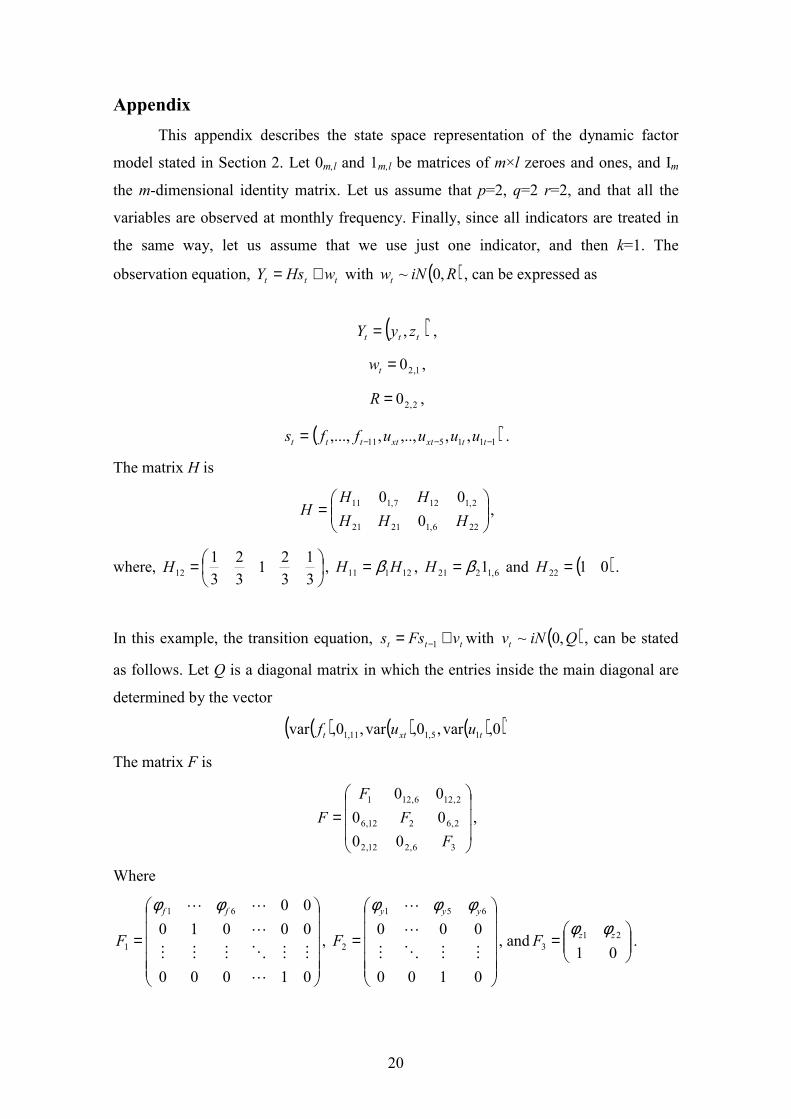
Appendix
This appendix describes the state space representation of the dynamic factor
model stated in Section 2. Let 0m,l and 1m,l be matrices of m×l zeroes and ones, and Im
the m-dimensional identity matrix. Let us assume that p=2, q=2 r=2, and that all the
variables are observed at monthly frequency. Finally, since all indicators are treated in
the same way, let us assume that we use just one indicator, and then k=1. The
observation equation, ttt wHsY += with ( )Ri�wt ,0~ , can be expressed as
( )', ttt zyY = ,
1,20=tw ,
2,20=R ,
( )'111511 ,,,..,,,..., −−−= ttxtxtttt uuuuffs .
The matrix H is
=
226,12121
2,1127,111
0
00
HHH
HHH ,
where,
=3
1
3
21
3
2
3
112H , 12111 HH β= , 6,1221 1β=H and ( )0122 =H .
In this example, the transition equation, ttt vFss += −1 with ( )Qi�vt ,0~ , can be stated
as follows. Let Q is a diagonal matrix in which the entries inside the main diagonal are
determined by the vector
( ) ( ) ( )( )'15,111,1 0,var,0,var,0,var txtt uuf
The matrix F is
=
36,212,2
2,6212,6
2,126,121
00
00
00
F
F
F
F ,
Where
=
01000
00010
0061
1
L
MMOMMM
L
LL ff
F
φφ
,
=
0100
000
651
2MMOM
L
L yyy
F
φφφ
, and
=
01
21
3
zzF
φφ.

21
Table 1. Data description
Indicators Selected for the Spain-STING Model:
Variable Acronyms Source Periodicity/
Indicator Sample
Reporting
Lags
GDP growth GDP SSI Quarterly/Hard 1992.1-2008.4 +45 days
Industrial Production
Index (excl.. energy)
IPI SSI Monthly/Hard 1993.01-2008.11 +35days
Total Sales of Large
Firms
Sales AT Monthly/Hard 1996.01-2008.11 +32 days
Social Security
Contributors
SSC ML Monthly/Hard 1996.01-2008.12 0
Retail Sales Confident
Indicator
RS EC Monthly/Soft 1990.01-2008.12 0
Services Purchasing
Managers Index
PMI Serv. ISM Monthly/Soft 1999.08-2008.12 +2 days
Industrial Confident
Indicator
ICI EC Monthly/Soft 1990.01-2008.12 0
Imports Imports ME Monthly/Hard 1992.01-2008.10 +50days
Exports
Exports ME Monthly/Hard 1992.01-2008.10 +50days
Overnight Stays (Nights
Spent by foreigners in hotels)
Stays SSI Monthly/Hard 1991.01-2008.11 +23 days
Cement Consumption Cement CPA Monthly/Hard 1992.01-2008.10 Not a fix
date
Notes. SSI refers to Spanish Statistical Institute, AT refers to Agencia Tributaria (Spanish
IRS), ML refers to Ministry of Labor, EC refers to European Commission, ISM referst to
Institute for Supply Management, ME refers to Ministry of Economy, and CPA refers to
Cement Producers Association.

22
Table 2. Data set available on the day of the forecast
GDP ICI RS PMI IPI Sales Exports Imports Stays Cement SSC
2008.06 0.15 -17.10 -24.70 36.70 -10.26 -9.67 -4.75 -4.22 -2.15 -32.73 -0.07
2008.07 na -16.40 -25.60 37.10 -5.31 -6.25 6.65 -2.81 0.88 -26.50 -0.52
2008.08 na -17.50 -35.40 39.00 -8.43 -6.58 2.75 -2.10 -1.33 -24.32 -0.85
2008.09 -0.24 -22.10 -32.90 36.10 -10.27 -8.50 8.50 -4.39 -1.84 -30.06 -1.48
2008.10 na -27.20 -29.80 32.20 -13.79 -11.32 0.33 -12.34 -4.54 -33.65 -2.41
2008.11 na -32.60 -26.20 28.20 -16.73 -13.21 na na -10.71 na -3.43
2008.12 na -37.60 -33.90 32.10 na na na na na na -4.32
2009.01 na na na na na na na na na na na
2009.02 na na na na na na na na na na na
2009.03 na na na na na na na na na na na
2009.04 na na na na na na na na na na na
2009.05 na na na na na na na na na na na
2009.06 na na na na na na na na na na na
Notes. See Table 1 for acronyms. Figures labelled as “na” refer to either missing data or
data that are not available on the day of the forecast.
Table 3. Factor loadings
GDP ICI RS PMI IPI Sales Exports Imports Stays Cement SSC0.13 0.05 0.03 0.05 0.07 0.06 0.01 0.04 0.02 0.05 0.06
(0.04) (0.01) (0.01) (0.02) (0.02) (0.02) (0.01) (0.01) (0.01) (0.02) (0.02)
Notes. See Table 1 for acronyms. Standard errors are in parentheses. Data set ends in
December 2008.

23
Table 4. Model-based forecasts
Panel A Panel B
Series 2008.4 2009.1 2009.2 Series Next Month
ICI -40.32
GDP -0.92 -0.91 -0.80 RS -33.79
(0.19) (0.22) (0.25) PMI 29.47
IPI -18.46
Sales -14.95
Exports 3.12
Imports -11.77
Stays -8.77
Cement -36.05
SSC -4.78
Notes. See Table 1 for acronyms. Standard errors are in parentheses. Data set ends on
December 2008.
Table 5. Cumulative weights
GDP ICI RS PMI IPI Sales ExportsImports Stays Cement SSC
2008.06 1.00 0.00 0.00 0.00 0.00 0.00 0.00 0.00 0.00 0.00 0.002008.07 0.00 0.04 0.02 0.08 0.05 0.45 0.01 0.05 0.01 0.09 0.212008.08 0.00 0.03 0.02 0.08 0.05 0.47 0.01 0.05 0.01 0.08 0.202008.09 1.00 0.00 0.00 0.00 0.00 0.00 0.00 0.00 0.00 0.00 0.002008.10 0.00 0.04 0.02 0.08 0.05 0.45 0.01 0.05 0.01 0.09 0.212008.11 0.00 0.04 0.02 0.09 0.05 0.56 0.00 0.00 0.01 0.00 0.232008.12 0.00 0.10 0.06 0.24 0.00 0.00 0.00 0.00 0.00 0.00 0.602009.01 0.00 0.00 0.00 0.00 0.00 0.00 0.00 0.00 0.00 0.00 0.002009.02 0.00 0.00 0.00 0.00 0.00 0.00 0.00 0.00 0.00 0.00 0.002009.03 0.00 0.00 0.00 0.00 0.00 0.00 0.00 0.00 0.00 0.00 0.002009.04 0.00 0.00 0.00 0.00 0.00 0.00 0.00 0.00 0.00 0.00 0.002009.05 0.00 0.00 0.00 0.00 0.00 0.00 0.00 0.00 0.00 0.00 0.002009.06 0.00 0.00 0.00 0.00 0.00 0.00 0.00 0.00 0.00 0.00 0.00
Notes. See Table 1 for acronyms. Data set ends on 02/11/08.

24
Figure 1. Time series used in the model
-1.5
-0.5
0.5
1.5
92.1 94.1 96.1 98.1 00.1 02.1 04.1 06.1 08.1
Sample 92.1-08.3
Sample 99.08-08.12
GDP growth rate
Production Manufacture Index
Industrial Production Total Sales of Large Firms
Sample 93.01-08.11 Sample 95.01-08.11
Sample 90.01-08.12
-50
-30
-10
10
90.01 92.08 95.03 97.10 00.05 02.12 05.07 08.02
Retail Sales Index
30
40
50
60
70
90.01 92.05 94.09 97.01 99.05 01.09 04.01 06.05 08.09
-15
0
15
90.01 92.05 94.09 97.01 99.05 01.09 04.01 06.05 08.09
-15
0
15
90.01 92.05 94.09 97.01 99.05 01.09 04.01 06.05 08.09
-50
-30
-10
10
90.01 92.08 95.03 97.10 00.05 02.12 05.07 08.02
Industrial Confident Indicator
Sample 90.01-08.12

25
Figure 1. Time series used in the model (continued)
Exports
Sample 92.01-08.10
-10
10
30
90.01 92.05 94.09 97.01 99.05 01.09 04.01 06.05 08.09
Imports
Sample 99.01-08.10
-20
0
20
40
90.01 92.08 95.03 97.10 00.05 02.12 05.07 08.02
Imports
-20
0
20
40
90.01 92.08 95.03 97.10 00.05 02.12 05.07 08.02
Sample 92.01-08.10
Imports
-20
0
20
40
90.01 92.05 94.09 97.01 99.05 01.09 04.01 06.05 08.09
Sample 91.01-08.11
Overnight Stays
-20
0
20
40
90.01 92.05 94.09 97.01 99.05 01.09 04.01 06.05 08.09
Sample 92.01-08.10
Apparent Consumption of Cement
-35
-15
5
25
90.01 92.08 95.03 97.10 00.05 02.12 05.07 08.02
Sample 96.01-08.12
Social Security Contributions
-5
0
5
90.01 92.08 95.03 97.10 00.05 02.12 05.07 08.02
Notes. GDP is in quarterly growth rates. Soft indicators are in levels. Hard indicators are
in annual growth rates.

26
Figure 2. Common factor and Indicador Sintético de Actividad
Notes. The factor (bottom line) is estimated from 91.01 to 09.06 with information in
December 2008. Top line refers to the annual growth rates of Indice Sintético de
Actividad. Dotted line refers to the averaged value.
-12
-9
-6
-3
0
3
6
90.01 92.10 95.07 98.04 01.01 03.10 06.07 09.04
Figure 3. GDP second growth rate: actual and estimates
Notes. GDP growth rates are estimated from 91.01 to 09.06 with information on
December 2008. Dots over this line refer to actual data (third month of each quarter; last
one in 2008.3). Dotted line refers to the averaged value.
-1.8
-1
-0.2
0.6
1.4
90.01 92.11 95.09 98.07 01.05 04.03 07.01

27
Figure 4. GDP forecast in 2009.1 and IPI potential releases
Notes. Potential releases of IPI in annual growth rates and their associated expected GDP
growth rate for 2009.1. Actual IPI was -16.73 which refer to an expected growth rate of -0.91.
-1.2
-0.9
-0.6
-0.3
0
-30 -10 10 30
Potential IPI realizations
Expected GDP growth rate
-0.91
-16.73
Figure 5. Real time growth rates forecasts for 2008Q1, 2008Q2, 2008Q3 and 2008Q4
20/02/2008 – 25/01/2009
-1.2
-0.8
-0.4
0
0.4
0.8
20/02/2008 31/03/2008 10/05/2008 19/06/2008 29/07/2008 07/09/2008 17/10/2008 26/11/2008 05/01/2009
2008Q1 2008Q2 2008Q3 2008Q4 zero line
GDPQ1 GDPQ2 GDPQ3 GDPQ4
Notes. The figure plots the real time forecast of growth rates of GDP and its realization. For
example, the green thick line shows the forecast for the fourth quarter of GDP from the first
day in which the model produces the forecasts (20/02/2008). The thin green horizontal line is
the realization.

AR forecasts
Spain-STING forecasts
20/02/2008 12/04/2008 03/06/2008 25/07/2008 15/09/2008 06/11/2008
-0.4
-0.05
0.3
0.65
1
GDP 2008.3
Notes. Spain-STING forecasts are calculated each day of the nine-month forecasting
periods described in the text. Shaded area refers to one standard error bands. Top and
bottom lines refer to AR (2) forecasts and actual GDP, respectively.
28
Figure 6. Real time forecast of growth rate for 2008.3