Embed Size (px)
Citation preview
Diss. ETH No. 20013
Sparse Convex Optimization
Methods for Machine Learning
A dissertation submitted to
ETH Zurich
for the degree of
Doctor of Sciences
presented by
Martin JaggiDipl. Math. ETH
born Mai 23, 1982
citizen of Lenk BE, Switzerland
accepted on the recommendation of
Prof. Dr. Emo Welzl, examiner
Dr. Bernd Gartner, co-examiner
Dr. Elad Hazan, co-examiner
Prof. Dr. Joachim Giesen, co-examiner
Prof. Dr. Joachim M. Buhmann, co-examiner
2011

Abstract
Convex optimization is at the core of many of today’s analysis tools forlarge datasets, and in particular machine learning methods. In this the-sis we will study the general setting of optimizing (minimizing) a convexfunction over a compact convex domain.
In the first part of this thesis, we study a simple iterative approximationalgorithm for that class of optimization problems, based on the classicalmethod by Frank & Wolfe. The algorithm only relies on supporting hy-perplanes to the function that we need to optimize. In each iteration,we move slightly towards a point which (approximately) minimizes thelinear function given by the supporting hyperplane at the current point,where the minimum is taken over the original optimization domain. Incontrast to gradient-descent-type methods, this algorithm does not needany projection steps in order to stay inside the optimization domain.
Our framework generalizes the sparse greedy algorithm of Frank & Wolfeand its recent primal-dual analysis by Clarkson (and the low-rank SDPapproach by Hazan) to arbitrary compact convex domains. Analogously,we give a convergence proof guaranteeing ε-small error — which in ourcontext is the duality gap — after O( 1
ε ) iterations.This method allows us to understand the sparsity of approximate so-
lutions for any `1-regularized convex optimization problem (and for opti-mization over the simplex), expressed as a function of the approximationquality. Here we obtain matching upper and lower bounds of Θ
(1ε
)for the
sparsity. The same bounds apply to low-rank semidefinite optimizationwith bounded trace, showing that rank O
(1ε
)is best possible here as well.
For some classes of geometric optimization problems, our algorithm hasa simple geometric interpretation, which is also known as the coreset con-cept. Here we will study linear classifiers such as support vector machines(SVM) and perceptrons, as well as general distance computations betweenconvex hulls (or polytopes). Here the framework will allow us to under-stand the sparsity of SVM solutions, here being the number of supportvectors, in terms of the required approximation quality.
iii
For matrix optimization problems, we show that our proposed first-order method also applies to convex optimization over bounded nuclearnorm or max-norm. This class of optimization problems has prominentapplications in several areas, such as low-rank recovery, matrix completionand recommender systems. We demonstrate the practical efficiency andscalability of our algorithm for large matrix problems, as e.g. the Netflixdataset. For general convex optimization over bounded matrix max-norm,our algorithm is the first with a convergence guarantee, to the best of ourknowledge.
In the last part of this thesis, we will consider convex optimization prob-lems which are parameterized by a single additional parameter, as for ex-ample a time or regularization parameter. In several applications, one isinterested in the entire path of the solution, as the parameter changes.
Here, a continuity argument together with our simple concept of opti-mization duality for compact domains will allow us to obtain solution paths(of some guaranteed approximation quality) for such problems. We showthat piecewise constant solutions can be obtained, and that O
(1ε
)many
such solutions are enough in order to guarantee approximation quality εalong the entire path, independent of the dimension of the problem. Ourmethod allows us to compute solution paths for e.g. SVMs, `1- or `∞-regularized problems, nuclear norm regularized problems such as matrixcompletion, and robust principal component analysis.
iv
Zusammenfassung
Konvexe Optimierung steht im Mittelpunkt von vielen der heute ver-fugbaren Analyse-Methoden fur grosse Datenmengen, insbesondere vonMethoden des maschinellen Lernens. In dieser Arbeit untersuchen wir dasallgemeine Problem der Optimierung (bzw Minimierung) einer konvexenFunktion uber einem kompakten konvexen Gebiet.
Im ersten Teil dieser Arbeit untersuchen wir einen einfachen iterativenAlgorithmus fur diese Klasse von Optimierungsproblemen, basierend aufder klassischen Methode von Frank & Wolfe. Der Algorithmus benutztstutzende Hyperebenen der zu optimierenden Funktion. In jeder Iterationbewegen wir uns etwas in die Richtung eines Punktes, welcher die lineareFunktion gegeben durch eine momentane stutzende Ebene (annahernd)minimiert, wobei das Minimum uber das ursprungliche Optimierungs-Gebiet genommen wird. Im Gegensatz zu Gradienten-Abstiegs-Methodenbenotigt dieser Algorithmus keine Projektions-Schritte, um innerhalb deszulassigen Gebiets zu bleiben.
Unser Ansatz verallgemeinert den Sparse-Greedy-Algorithmus von Frank& Wolfe und seine neuere primal-duale Analysis durch Clarkson (sowie diesemi-definite Optimierungsmethode mittels kleinem Rang von Hazan) aufbeliebige kompakte konvexe Gebiete. Unser Konvergenz-Beweis garantiertε-kleinen Fehler (Dualitats-Lucke) nach O
(1ε
)Iterationen.
Die Methode ermoglicht es uns die Dunnbesetztheit (Sparsity) von ap-proximativen Losungen fur `1-regularisierte konvexe Optimierungs-Prob-leme (und fur die Optimierung uber dem Simplex), als Funktion der Appro-ximations-Gute zu verstehen. Hier erhalten wir passende obere und untereSchranken von Θ
(1ε
)fur die Dunnbesetztheit. Die gleichen Grenzen gelten
fur semi-definite Optimierung unter beschrankter Spur, in Bezug auf denMatrix-Rang. Hier zeigen wir dass Rang O
(1ε
)ebenfalls optimal ist.
Fur einige Klassen von geometrischen Optimierungsproblemen hat unserAlgorithmus eine einfache geometrische Interpretation, die auch als dasKonzept der Coresets bekannt ist. Hier untersuchen wir lineare Klassi-fikatoren wie zum Beispiel Support Vector Machines (SVM), sowie all-gemeine Entfernungsberechnungen zwischen konvexen Hullen (oder Poly-
v
topen). Hier ermoglicht unser Framework die Dunnbesetztheit der SVM-Losungen zu verstehen, was in diesem Zusammenhang die Anzahl derSupport-Vektoren bedeutet, in Abhangigkeit der erforderlichen Approxi-mations-Gute.
Unsere Methode ist ebenfalls direkt anwendbar fur Matrix-Optimie-rungs-Probleme, insbesondere fur konvexe Optimierung unter beschrank-ter Spur-Norm oder Max-Norm. Diese Klasse von Optimierungsproblemenhat prominente Anwendungen in verschiedenen Bereichen, wie z.B. dieRekonstruktion von Matrizen von kleinem Rang, oder die Komplettierungvon Matrizen zum Beispiel bei Empfehlungs-Systemen. Wir demonstrierendie praktische Effizienz und Skalierbarkeit unseres Algorithmus fur grosseMatrix-Probleme, wie z.B. dem Netflix-Datenset. Fur allgemeine konvexeOptimierung unter beschrankter Matrix Max-Norm ist unser Algorithmusnach unserem Wissen die erste Methode mit einer Konvergenz-Garantie.
Im letzten Teil dieser Arbeit betrachten wir konvexe Optimierungspro-bleme die von einem zusatzlichen Parameter abhangen, wie z.B. einemZeit- oder Regularisierungs-Parameter. In einigen Anwendungen ist manam gesamten Pfad der Losung interessiert, in Abhangigkeit des zusatzlichenParameters.
Mittels eines Stetigkeits-Arguments, zusammen mit unserem einfachenalternativen Konzept der Dualitat fur Optimierung uber kompaktem Ge-biet, erhalten wir die vollstandigen Losungspfade (fur eine garantierteApproximations-Gute) fur solche Probleme. Wir zeigen, dass stuckweisekonstante Losungen existieren, und dass O
(1ε
)viele solcher Losungen ge-
nugen, um eine Approximations-Gute von ε entlang dem gesamten Pfadzu garantieren, unabhangig von der Dimension des Problems. UnsereMethode erlaubt das Berechnen von Losungspfaden fur z.B. SVMs, `1-oder `∞-regularisierte Probleme, Spur-Norm-regularisierte Probleme wieMatrix-Komplettierung, sowie robuste Hauptkomponentenanalyse (PCA).
vi
Acknowledgments
I would like to express my gratitude to my advisor Bernd Gartner. Withouthis continuous support, openness and patience, this thesis would never havebeen written. I am also very grateful to Emo Welzl for letting me be partof his research group, and for providing a working environment that couldnot possibly be any better.
Furthermore I would like to thank Joachim Giesen for sparking my inter-est in support vector machines, for the collaboration on path algorithms,for inviting me to Saarbrucken and Jena, and for co-refereeing this thesis.
Many thanks to Elad Hazan and Joachim Buhmann for agreeing to beco-examiners and for providing many helpful comments. For the researchcollaboration, I would like to thank Soeren Laue and Marek Sulovsky.
All members of the Gremo team made the time at ETH unforgettable:Andrea Francke, Andrea Salow, Anna Gundert, Heidi Gebauer, MichaelHoffmann, Robin Moser, Sebastian Stich, Timon Hertli, Uli Wagner, Vin-cent Kusters, Yves Brise, as well as all former members whom I had thepleasure to meet: Tobias Christ, Gabriel Nivasch, Marek Sulovsky, Do-minik Scheder, Floris Tschurr, Patrick Traxler, Andreas Razen, PhilippZumstein, Tibor Szabo, Robert Berke, Eva Schuberth, and Leo Rust.
I am indebted to Heidi, Tobias and Sebastian for proof-reading partsof this thesis, and to Robert Carnecky for the 3d visualization of con-vex minimization. For helpful and inspiring discussions and support, Iwould like to thank Andreas Krause, Arkadi Nemirovski, Christian LorenzMuller, Christoph Krautz, Clement Maria, Florian Jug, Gabriel Katz,Mark Cieliebak, Michael Burgisser, Michel Baes, Michel Verlinden, PankajAgarwal, Simon Meier and Yves Ineichen.
For gently introducing me to some real-world machine learning appli-cations, I am very grateful to Daniel Mahler, Hartmut Maennel and LarsEngebretsen from Google, and to Francois Ruf from Netbreeze.
I want to thank all friends, WG-gspanli and climbing partners, to ETHmensa for roughly a decade of calories, and to Minimum and Milandia forall the nicely arranged colorful plastic holds.
Last but not least I want to thank my family for always being there, myparents Theres and Walter, my brother Thomas; and Nadja for her loveand understanding.
vii

Contents
1. Introduction 11.1. Convex Optimization . . . . . . . . . . . . . . . . . . . . . . . . . 21.2. Sparsity and Generalizations Thereof . . . . . . . . . . . . . . . . 31.3. Regularization Methods . . . . . . . . . . . . . . . . . . . . . . . 5
1.3.1. Least Squares Regression . . . . . . . . . . . . . . . . . . 61.3.2. Two equivalent Variants of Regularization . . . . . . . . . 71.3.3. Linear Classifiers and Support Vector Machines . . . . . . 8
1.4. Geometric Problems . . . . . . . . . . . . . . . . . . . . . . . . . 91.5. Solution Path Methods . . . . . . . . . . . . . . . . . . . . . . . . 101.6. Notation and Terminology . . . . . . . . . . . . . . . . . . . . . . 11
2. Convex Optimization without Projection Steps 132.1. Introduction . . . . . . . . . . . . . . . . . . . . . . . . . . . . . . 132.2. The Poor Man’s Approach to Convex Optimization and Duality 17
2.2.1. Subgradients of a Convex Function . . . . . . . . . . . . . 172.2.2. A Duality for Convex Optimization over Compact Domain 18
2.3. A Projection-Free First-Order Method for Convex Optimization . 202.3.1. The Algorithm . . . . . . . . . . . . . . . . . . . . . . . . 202.3.2. Obtaining a Guaranteed Small Duality Gap . . . . . . . . 262.3.3. Choosing the Optimal Step-Size by Line-Search . . . . . . 282.3.4. The Curvature Measure of a Convex Function . . . . . . . 292.3.5. Optimizing over Convex Hulls . . . . . . . . . . . . . . . . 322.3.6. Randomized Variants, and Stochastic Optimization . . . . 332.3.7. Relation to Classical Convex Optimization . . . . . . . . 34
3. Applications to Sparse and Low Rank Approximation 373.1. Sparse Approximation over the Simplex . . . . . . . . . . . . . . 37
3.1.1. Upper Bound: Sparse Greedy on the Simplex . . . . . . . 393.1.2. Ω( 1
ε) Lower Bound on the Sparsity . . . . . . . . . . . . . 41
3.2. Sparse Approximation with Bounded `1-Norm . . . . . . . . . . . 433.2.1. Relation to Matching Pursuit and Basis Pursuit in Com-
pressed Sensing . . . . . . . . . . . . . . . . . . . . . . . . 473.3. Optimization with Bounded `∞-Norm . . . . . . . . . . . . . . . 483.4. Semidefinite Optimization with Bounded Trace . . . . . . . . . . 50
3.4.1. Low-Rank Semidefinite Optimization with Bounded Trace:The O( 1
ε) Algorithm by Hazan . . . . . . . . . . . . . . . 51
3.4.2. Solving Arbitrary SDPs . . . . . . . . . . . . . . . . . . . 57
ix
Contents
3.4.3. Two Improved Variants of Algorithm 6 . . . . . . . . . . 583.4.4. Ω( 1
ε) Lower Bound on the Rank . . . . . . . . . . . . . . 59
3.5. Semidefinite Optimization with `∞-Bounded Diagonal . . . . . . 613.6. Sparse Semidefinite Optimization . . . . . . . . . . . . . . . . . . 643.7. Submodular Optimization . . . . . . . . . . . . . . . . . . . . . . 67
4. Optimization with the Nuclear and Max-Norm 694.1. Introduction . . . . . . . . . . . . . . . . . . . . . . . . . . . . . . 694.2. The Nuclear Norm for Matrices . . . . . . . . . . . . . . . . . . . 74
4.2.1. Weighted Nuclear Norm . . . . . . . . . . . . . . . . . . . 764.3. The Max-Norm for Matrices . . . . . . . . . . . . . . . . . . . . . 774.4. Optimizing with Bounded Nuclear Norm and Max-Norm . . . . . 79
4.4.1. Optimization with a Nuclear Norm Regularization . . . . 804.4.2. Optimization with a Max-Norm Regularization . . . . . . 82
4.5. Applications . . . . . . . . . . . . . . . . . . . . . . . . . . . . . . 844.5.1. Robust Principal Component Analysis . . . . . . . . . . . 844.5.2. Matrix Completion and Low Norm Matrix Factorizations 854.5.3. The Structure of the Resulting Eigenvalue Problems . . . 884.5.4. Relation to Simon Funk’s SVD Method . . . . . . . . . . 89
4.6. Experimental Results . . . . . . . . . . . . . . . . . . . . . . . . . 904.7. Conclusion . . . . . . . . . . . . . . . . . . . . . . . . . . . . . . 92
5. A Geometric Optimization Method, and Coresets for Polytope Distanceand SVMs 955.1. Introduction . . . . . . . . . . . . . . . . . . . . . . . . . . . . . . 965.2. Concepts and Definitions . . . . . . . . . . . . . . . . . . . . . . 99
5.2.1. Polytope Distance . . . . . . . . . . . . . . . . . . . . . . 995.2.2. Distance Between Two Polytopes . . . . . . . . . . . . . . 1005.2.3. Relation to our General Setting of Convex Optimization
Over Bounded Domain . . . . . . . . . . . . . . . . . . . . 1015.3. Lower Bounds on the Sparsity of ε-Approximations . . . . . . . . 103
5.3.1. Distance of One Polytope from the Origin . . . . . . . . . 1035.3.2. Distance Between Two Polytopes . . . . . . . . . . . . . . 105
5.4. Upper Bounds: Algorithms to Construct Coresets . . . . . . . . . 1085.4.1. Gilbert’s Algorithm . . . . . . . . . . . . . . . . . . . . . 1085.4.2. An Improved Version of Gilbert’s Algorithm for Two Poly-
topes . . . . . . . . . . . . . . . . . . . . . . . . . . . . . . 1125.4.3. Smaller Coresets by “Away” Steps . . . . . . . . . . . . . 117
5.5. Applications to Machine Learning . . . . . . . . . . . . . . . . . 1185.5.1. Sparsity of SVM and Perceptron Solutions . . . . . . . . . 1195.5.2. Linear Time Training of SVMs and Perceptrons . . . . . . 121
6. Solution Paths for Convex Optimization Problems over Vectors 1236.1. Introduction . . . . . . . . . . . . . . . . . . . . . . . . . . . . . . 123
x
Contents
6.2. Approximation Quality Measures . . . . . . . . . . . . . . . . . . 1266.3. Optimizing Parameterized Functions . . . . . . . . . . . . . . . . 128
6.3.1. Stability of ε-Approximations . . . . . . . . . . . . . . . . 1296.3.2. Bounding the Path Complexity . . . . . . . . . . . . . . . 1306.3.3. Lower Bound . . . . . . . . . . . . . . . . . . . . . . . . . 1316.3.4. Relative Approximation . . . . . . . . . . . . . . . . . . . 1336.3.5. The Weighted Sum of Two Convex Functions . . . . . . . 133
6.4. Applications . . . . . . . . . . . . . . . . . . . . . . . . . . . . . . 1366.4.1. A Parameterized Polytope Distance Problem . . . . . . . 1366.4.2. The Regularization Path of Support Vector Machines . . 1396.4.3. Multiple Kernel Learning . . . . . . . . . . . . . . . . . . 1416.4.4. Minimum Enclosing Ball of Points under Linear Motion . 142
6.5. Experimental Results . . . . . . . . . . . . . . . . . . . . . . . . . 1436.5.1. The Regularization Path of Support Vector Machines . . 1436.5.2. Multiple Kernel Learning . . . . . . . . . . . . . . . . . . 145
6.6. Conclusion . . . . . . . . . . . . . . . . . . . . . . . . . . . . . . 147
7. Solution Paths for Semidefinite Optimization 1497.1. Introduction . . . . . . . . . . . . . . . . . . . . . . . . . . . . . . 1507.2. The Duality Gap . . . . . . . . . . . . . . . . . . . . . . . . . . . 1537.3. Optimizing Parameterized Semidefinite Problems . . . . . . . . . 154
7.3.1. Computing Approximate Solution Paths . . . . . . . . . . 1577.3.2. Plugging-in Existing Methods for Semidefinite Optimization158
7.4. Applications . . . . . . . . . . . . . . . . . . . . . . . . . . . . . . 1597.4.1. Matrix Completion . . . . . . . . . . . . . . . . . . . . . . 1597.4.2. Solution Paths for the Weighted Nuclear Norm . . . . . . 1607.4.3. Solution Paths for Robust PCA . . . . . . . . . . . . . . . 1607.4.4. Solution Paths for Sparse PCA and Maximum Variance
Unfolding . . . . . . . . . . . . . . . . . . . . . . . . . . . 1617.5. Experimental Results . . . . . . . . . . . . . . . . . . . . . . . . . 1627.6. Conclusion . . . . . . . . . . . . . . . . . . . . . . . . . . . . . . 164
A. Optimization Basics 165A.1. Constrained Optimization Problems over Vectors . . . . . . . . . 165A.2. Matrix Optimization Problems & Generalized Inequality Con-
straints . . . . . . . . . . . . . . . . . . . . . . . . . . . . . . . . 166A.3. Convex Optimization and the Wolfe Dual . . . . . . . . . . . . . 167A.4. Convex Optimization over the Simplex . . . . . . . . . . . . . . . 169A.5. Convex Optimization with `∞-Norm Regularization . . . . . . . 171A.6. Semidefinite Optimization with Bounded Trace . . . . . . . . . . 172A.7. Semidefinite Optimization with `∞-Bounded Diagonal . . . . . . 175
Bibliography 179
xi


1Introduction
With the immense growth of available digital data, algorithmic analysistechniques for large datasets have become increasingly important. The effi-ciency and scalability of many such techniques, in particular from the areaof machine learning, is often limited by the currently available methods tosolve the underlying convex optimization problems.
Machine Learning. In an informal sense, machine learning is the taskof building a model for some quantity (or function) that we would like topredict, or in other words, learn. The model is usually built from a set of“training” data for which the corresponding quantity of interest is known.Later, the obtained model is used to predict on new or unknown data,where we will then evaluate the performance of the obtained model. Sofar, this task description strikingly resembles classical regression, which isnot a coincidence.
Concrete practical examples of such machine learning questions includeclassifying handwritten characters, reconstructing radio signals from verynoisy sources, detecting a disease from MRI brain images, recommendingmovies or other products depending on personal ratings given to otheritems, ranking websites in a search engine based on their text content,modeling the terrain from the data from the sensor of an autonomous car,and predicting climate parameters or stock prices based on historical data,as well as many other applications.
1
2 Introduction
1.1. Convex Optimization
The first part of this thesis addresses the general topic of convex opti-mization over bounded domains. Such convex optimization problems haveapplications in a very large variety of different areas, such as signal pro-cessing, computational biology, control theory, combinatorial optimization,communications and networking, statistics, finance, data mining, and —last but not least — in machine learning.
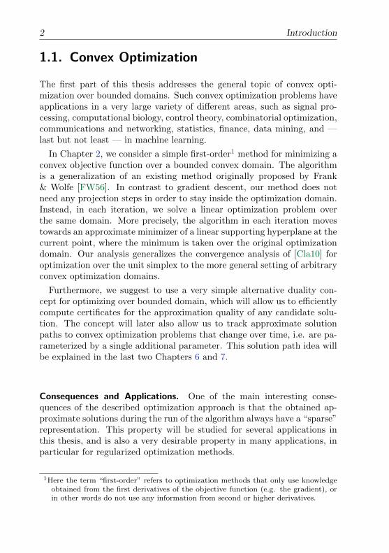
In Chapter 2, we consider a simple first-order1 method for minimizing aconvex objective function over a bounded convex domain. The algorithmis a generalization of an existing method originally proposed by Frank& Wolfe [FW56]. In contrast to gradient descent, our method does notneed any projection steps in order to stay inside the optimization domain.Instead, in each iteration, we solve a linear optimization problem overthe same domain. More precisely, the algorithm in each iteration movestowards an approximate minimizer of a linear supporting hyperplane at thecurrent point, where the minimum is taken over the original optimizationdomain. Our analysis generalizes the convergence analysis of [Cla10] foroptimization over the unit simplex to the more general setting of arbitraryconvex optimization domains.
Furthermore, we suggest to use a very simple alternative duality con-cept for optimizing over bounded domain, which will allow us to efficientlycompute certificates for the approximation quality of any candidate solu-tion. The concept will later also allow us to track approximate solutionpaths to convex optimization problems that change over time, i.e. are pa-rameterized by a single additional parameter. This solution path idea willbe explained in the last two Chapters 6 and 7.
Consequences and Applications. One of the main interesting conse-quences of the described optimization approach is that the obtained ap-proximate solutions during the run of the algorithm always have a “sparse”representation. This property will be studied for several applications inthis thesis, and is also a very desirable property in many applications, inparticular for regularized optimization methods.
1Here the term “first-order” refers to optimization methods that only use knowledgeobtained from the first derivatives of the objective function (e.g. the gradient), orin other words do not use any information from second or higher derivatives.
Sparsity and Generalizations Thereof 3
1.2. Sparsity and Generalizations Thereof
Suppose we are given a convex optimization problem, namely that we needto minimize a convex function over Rn. In many practical situations, wewould not only like to have any (approximate) solution, but we want asolution which has the additional property that it is also sparse, or inother words contains just few non-zero coordinates, say just k < n manyof these.
Unfortunately, the additional requirement of sparsity immediately turnsthe original convex problem (for which efficient algorithms are known)into a very hard combinatorial problem. Solving it would require us to tryall possible patterns of
(nk
)non-zeros in a brute-force way, requiring time
exponential in k. Also note that the set of sparse vectors (at most k manynon-zero coordinates) is not a convex set anymore.
Convex Relaxations by Using the `1-Norm. To allow for more efficientconvex optimization approaches, we need the domain to be a convex set.In the literature, a widely successful approach has been to replace therequirement of sparsity by optimizing over the `1-ball instead. The `1-ball is the set of all vectors in Rn, for which the absolute values of thecoordinates sum up to at most one (this quantity is known as the `1-norm). Also, it is not hard to see that the `1-ball is exactly the convexhull of the “sparsest possible” vectors, namely the standard basis vectors(and their negatives), i.e. the vectors with only one non-zero coordinate.
A Geometric Intuition. As one attempt to explain the usefulness of the`1-ball as a domain for obtaining sparse solutions, a simple geometric factcomes into play. It has been known for a very long time that for optimizingany linear function cTx over the `1-ball, there will always be a vertex ofthe ball where the optimum value is obtained. In other words there willalways be an optimal solution of the best possible sparsity.
This fact has been widely cited as the motivation to apply the verysame `1-relaxation trick as described above, also for the case of non-linearconvex optimization problems over Rn, when sparse solutions are desired.Intuitively, the hope is that also for these more general functions, optimiz-ing over the `1-ball would “often” return sparse solutions. More formally,one can show that the `1-norm is the convex function that best approxi-mates the sparsity.
4 Introduction
Sparsity as a Function of the Approximation Quality. In this thesis, wecan quantify this sparsity more precisely, by studying its dependency onthe desired approximation quality. We say that a point is an ε-approximatesolution to the optimization problem if its value is at least ε-close to theunknown true optimal value.
We show that if an approximation quality of ε > 0 is required, then thevery simple greedy algorithm that we described above will always providesparse solutions of only O
(1ε
)non-zero entries, if the optimization domain
is the `1-ball. The analysis will follow analogously to the result of [Cla10]for the unit simplex. Also, we provide an asymptotically matching lowerbound, that for some natural convex function, at least Ω
(1ε
)non-zero
entries are strictly necessary for any ε-approximate solution.This means we can characterize the sparsity as a function of the ap-
proximation quality. In other words, we have translated the fact thatevery linear optimization problem has a 1-sparse solution, to arbitrarynon-linear convex optimization problems, where we obtain O
(1ε
)-sparse
approximate solutions. This is particularly remarkable because we are notmaking any assumptions about the sparsity of the true optimal solution,which might be completely dense for example. Our approach is not limitedto the domain being the `1-ball or the unit simplex, but in fact works onevery bounded convex set, which is useful as follows:
Generalizing Sparsity to Description Complexity. Our generalized sparsegreedy optimization approach for arbitrary bounded convex domains willalso allow us to slightly generalize the concept of sparse solutions. For theconvex hull of arbitrary elements of some vector space, it is easy to seethat every linear function obtains its minimum at a vertex, or in otherwords one of the original “atomic” elements.
This implies that the algorithm will only ever use elements from the ini-tial “atoms” as the step direction in each iteration. In other words it willobtain an ε-approximate solution which is a convex combination (there-fore a weighted sum) of just O
(1ε
)many of the original atomic elements.
Alternatively we say that each obtained approximate solution has a lowdescription complexity, in terms of the elements defining the convex hull,which is our optimization domain. This idea is also closely related to therecent concept of structured sparsity, which refers to the same idea of mea-suring the complexity of an element in terms of e.g. how many atomicelements of some defined structure are needed to represent the element ofconsideration.
There are many interesting applications building upon such convex com-
Regularization Methods 5
binations of various objects. One prominent example is given by the sym-metric rank-1 matrices of unit trace, whose convex hull is known to be theset of all positive semidefinite matrices of bounded trace. In this example,we will recover the approach of Hazan [Haz08] for semidefinite optimiza-tion, and obtain solutions of rank O
(1ε
). This particular class of opti-
mization problems has many prominent examples e.g. in dimensionalityreduction, low-rank recovery, or recommender systems, as we will discussin more details in Chapter 4, where we will show how the algorithm can beused to solve arbitrary nuclear norm or max-norm constrained optimiza-tion problems over matrices.
Coresets. The coreset approach originally proposed in computational ge-ometry is another name for the same concept of sparse solutions for thecase of point set problems. Clarkson [Cla10] has already translated thisconcept to convex optimization over the unit simplex. Here we extend thisconcept also to convex optimization over bounded domains in arbitraryvector spaces.
1.3. Regularization Methods
In many real world applications, the available data is not perfect, butcontains small errors, additional noise, or other kinds of corruptions. Thisissue has only increased with the advancement of technology and the grow-ing amount of available data of all kinds, and proposes a significant chal-lenge for all methods to analyze and/or further process such data. Reg-ularization is widely used as a way to make existing techniques robust tonoise or corruptions in the data, and has seen many successful applications.Stephen Boyd and Emmanuel Candes, two of the leading researchers in thisarea, are referring to `1-regularized optimization methods as the “least-squares approach” of the 21st century, because of the simplicity and wideapplicability of such techniques.
One is probably tempted to think that in order to successfully attackmachine learning tasks (such as regression over noisy data), much morecomplex models would have to be used than for classical regression, say.However, the idea of regularization is in a sense exactly the opposite,namely that a model of small complexity should be used instead.
An Example. Here we will briefly introduce the regularization idea for aconcrete example, for two different methods of data analysis and machine
6 Introduction
learning. Suppose that we are given a set of m holiday pictures. We canrepresent each such digital image as a point xi ∈ Rn, being the large vectorconsisting of the numerical values (or colors) of each pixel of the image,stored one after each other. In other words x1, . . . , xm ∈ Rn are the pointsrepresenting the m pictures, and n is the number of pixels of our digitalcamera.
1.3.1. Least Squares Regression
We assume that for each holiday image xi, 1 ≤ i ≤ m, we are also given anumerical value yi describing how much we like that particular picture (sayon a scale from 1 to 5). We would like to “learn” or “fit” a linear functionto this data, so that we can later apply this function to a set of arbitraryimages (e.g. from Google image search), with the hope to automaticallyidentify the best suitable future holiday destination for our taste.
Formally, we now search for a linear function (described by a vectorω ∈ Rn) that minimizes the squared error
L(ω) :=
m∑i=1
(xTi ω − yi)2 = ‖Aω − y‖22 .
Here A ∈ Rm×n is the matrix that contains all our m datapoints xTi as itsrows, and y ∈ Rm is the vector consisting of the values yi that we wouldlike to approximate.
Now the convex optimization problem minω∈Rn L(ω) can definitely besolved efficiently. However, most solutions will very likely be totally mean-ingless, because the number of variables n is much higher than the numberof data points (m) that we have. In other words, since the system is ex-tremely under-determined, we will definitely suffer from the “curse of toomany parameters”. Changing only a single pixel in one of our holidaypictures will likely result in a totally different solution vector ω.
Here, regularization comes into play. The idea is that if there is anymeaningful solution (or model) ω to our problem at all, then that solutionshould be of small complexity. The same paradigm is known as Occam’srazor, that if there are several explanations for some phenomenon, then thesimplest one should be preferred. In our case, we will simply measure thecomplexity of each model ω by its `1-norm. Instead of solving the originalunconstrained optimization version minω∈Rn L(ω), we will now restrict toω being of small complexity, by constraining on a suitably scaled version
Regularization Methods 7
of the `1-ball, or formally
minω∈Rn‖ω‖1≤t
L(ω) . (1.1)
This formulation is called the `1-regularized version of the original (uncon-strained) least squares problem. Solutions to this problem tend to be muchmore meaningful for almost all applications where the available data is sub-ject to noise, or systems that have a very large number of free parameters.The question of what “suitable” means for the so called regularizationparameter t will be studied in Chapters 6 and 7 in more details.
Applying our simple greedy convex optimization procedure to `1-regu-larized least squares, we will obtain ε-approximate solutions ω which areadditionally sparse, i.e. have O
(1ε
)non-zero coordinates, which will be
explained in Chapter 2.
1.3.2. Two equivalent Variants of Regularization
As a small technical remark, we note that there are two equivalent vari-ants of adding regularization to a given original optimization problemminω∈Rn L(ω). Here we assume L(ω) is an arbitrary convex objective func-tion that we would like to optimize. If the model complexity of any ω ismeasured by a convex function R(ω), then the following two formulationsare equivalent. In machine learning terms, the function R(.) is usuallycalled the regularization term, while L(.) is called the loss function. Theconstrained variant of the regularized problem is given by
minω∈RnR(ω)≤t
L(ω) . (1.2)
The analogous trade-off version, for some trade-off parameter λ > 0 isgiven by
minω∈Rn
L(ω) + λR(ω) . (1.3)
The two parameters t and λ are in a direct correspondence. For choiceof λ > 0 together with some optimal solution ω(λ) to the trade-off vari-ant (1.3), setting t(λ) := R(ω(λ)) in the constrained variant (1.2) will resultin the same objective value L(ω(λ)) for the optimum of (1.2). On the otherhand, formulation (1.3) is also known as the Lagrangian version of (1.2).For any fixed t, there is always some choice of λ = λ(t) such that the op-timum of (1.3) has the same loss value L(ω(t)) as an optimal solution ω(t)
to (1.2).
8 Introduction
This direct correspondence between the solutions to the two problemvariants is the reason that both variants are used interchangeably in mostapplications of regularization methods. The following short section onlinear classifiers is an example where it is more common to work with thetrade-off variant (1.3).
1.3.3. Linear Classifiers and Support Vector Machines
As a second example, we would like to present linear classifiers. In the samesetting as for the holiday pictures x1, . . . , xm ∈ Rn as given in the abovesetting, we now consider classification instead of regression. This meansthat each of the pictures xi ∈ Rn comes together with a label yi ∈ ±1. Wethink of this label yi being +1 if the picture xi contains the face of someperson, and yi = −1 otherwise. We would like to find a linear classifierfor such images, or in other words we again search for a linear functionωTx determined by ω ∈ Rn, such that hopefully ωTxi > 0 for pictures xicontaining faces, and ωTxi < 0 otherwise. This approach is widely knownas the linear Perceptron.
Regularization and Support Vector Machines. It turns out that insteadof just solving the above constraints for some optimal ω, a much better andmore robust classifier ωTx is obtained by adding a regularization on thecomplexity of ω. Here, by a geometric interpretation that we will study inmore details in Chapter 5, the effect of the regularization will be that oneobtains a linear function that separates the datapoints not just in someway, but with the best possible margin of separation. This type of largemargin linear classifier is called the support vector machine (SVM).
The standard optimization problem for the linear SVM is given by
minω∈Rn
1
m
m∑i=1
(1− yiωTxi
)++ λ ‖ω‖22
Here the notation (.)+ returns the positive part of its argument, meaningthat (s)+ is equal to s for s ≥ 0, and zero otherwise. The interpretation of
the loss-term L(ω) := 1m
∑mi=1
(1− yiωTxi
)+is that all points which are
on their correct side of the hyperplane (given by ωTx = 0) and are at leastsome distance away from the plane, i.e. yiω
Txi > 1, will not contributeto the loss L(ω). All other points that are too close to the hyperplane —or do lie on the wrong side corresponding to the opposite label — will bepunished by the term L(ω).
Geometric Problems 9
For linear classifiers, the effect of the above regularization term ‖ω‖2 onthe resulting solution ω is well studied, and is equivalent to choosing theseparating hyperplane ω of the largest possible separation margin. It canbe shown this particular hyperplane indeed results in the best expectedprediction accuracy on unknown “test” data, where we only have to assumethat the test data is drawn from the same distribution as the “training”points (from which we have obtained the hyperplane). Results of thistype are often proven by using the concept of Rademacher complexity, seee.g. [STC04].
Also in this completely different optimization approach as comparedto our first example of `1-regularized regression, it turns out that theregularization idea (here by constraining ‖ω‖2 as compared to ‖ω‖1), is anextremely powerful tool in practice. For classification tasks, SVMs havebecome the basic tool of choice in most applications.
The idea of adding regularization to linear classifiers — and therebyalso enabling its application to “noisy” point sets that are not perfectlylinearly separable — was originally proposed by [CV95], and was awardedthe ACM Paris Kanellakis Theory and Practice Award in 2008.
Sparsity and the Number of Support Vectors. Using optimization dual-ity, it is not hard to see that every meaningful hyperplane for an SVM canbe expressed as a convex combination of the original datapoints. Applyingour simple greedy convex optimization procedure to SVMs, we will obtaincoresets (small sets of support vectors) of size O
(1ε
), see Chapter 5. We
also provide examples showing that this is best possible up to a constantfactor. This means we can understand the number of support vectors as afunction of the approximation quality ε.
1.4. Geometric Problems
In Chapter 5, we will study the geometric interpretation of the generalconvex optimization technique described above, for the case of computingdistances between convex hulls (or polytopes). This problem also appearsnaturally in collision detection for geometric objects in physical simulationsor computer games.
However, here we will focus mostly on applications to linear classifiers formachine learning applications, and in particular support vector machines(SVM) and perceptrons. As mentioned above, our method translates thecoreset concept to these problems, and allows us to understand the sparsity
10 Introduction
of SVM solutions, here being the number of support vectors.
1.5. Solution Path Methods
In the two last Chapters 6 and 7, we will study convex optimization prob-lems which are parameterized by a single additional parameter, as forexample a time or regularization parameter.
A continuity argument together with our simple proposed concept ofoptimization duality for compact domains will allow us to study solutionpaths (of some guaranteed approximation quality) for such problems. Weshow that piecewise constant solutions can be obtained, and that O
(1ε
)many such solutions are enough in order to guarantee approximation qual-ity ε along the entire path, independent of the dimension of the problem.
The entire path of solutions to a parameterized problem is interestingin many application areas, in particular for regularization methods as de-scribed above. Here the parameter of interest is the regularization param-eter t in (1.2), or λ in (1.3), and one would like to study the performanceof the solutions (such as e.g. the prediction quality on a separate set oftest data) for the continuous path of the solution, as the regularizationparameter changes. Other applications of such continuation or homotopymethods can be found e.g. in control theory.
Notation and Terminology 11
1.6. Notation and Terminology
Convexity. A subset D of some vector space is called convex, if for anychoice of two points a, b ∈ D, the line segment
[a, b] :=λa+ (1− λ)b
∣∣ 0 ≤ λ ≤ 1⊆ D
is also contained in D. A real-valued function D → R is called convex, if
f(λa+ (1− λ)b
)≤ λf(a) + (1− λ)f(b) ∀a, b ∈ D, 0 ≤ λ ≤ 1
or in other words the line segment connecting the function values at a andb must lie above the graph of the function f .
Spaces and Norms. Consider a vector space X equipped with an innerproduct 〈., .〉. As the most prominent example of such a space, the readermight always think of the standard n-dimensional Euclidean space X = Rnwith 〈x, y〉 = xT y being the standard scalar product.
For any norm ‖.‖ on X , the corresponding dual norm is defined by
‖x‖∗ := supy∈X ,‖y‖≤1
〈y, x〉 .
Vectors. For a vector x ∈ Rn, we write x ≥ 0 if and only if xi ≥ 0 ∀i holdscoordinate-wise. The sparsity, or cardinality, of x ∈ Rn, also written ascard(x), is the number of non-zero coordinates xi. The `1-norm of a vectoris defined as ‖x‖1 =
∑ni=1 |xi|. The standard Euclidean norm is given by
‖x‖2 =√∑n
i=1 x2i , and the max-norm is defined as ‖x‖∞ = maxni=1 |xi|.
Observe that ‖x‖∞ ≤ ‖x‖2 ≤ ‖x‖1.
Matrices. For real matrices in Rm×n, the standard inner product is de-fined as A • B := Tr(ATB), and the (squared) Frobenius matrix norm is
given by ‖A‖2Fro := A•A, the sum of all squared entries in the matrix. Wewill use of the fact that the inner product is symmetric, i.e. A•B = B •A,which equivalently means that Tr(ATB) = Tr(BTA).
We will sometimes write Ai: for the i-th row of a matrix A ∈ Rm×n, andA:j for the j-th column.
Sn×n is the set of symmetric n × n matrices. We write λmax(A) forthe largest eigenvalue of a matrix A ∈ Sn×n, and λmin(A) for the smallesteigenvalue respectively. A is called positive semidefinite (PSD), written asA 0, iff vTAv ≥ 0 ∀v ∈ Rn. We observe that vTAv = A • vvT .

2Convex Optimization
without Projection Steps
In this chapter, we study the general problem of minimizing a convexfunction over a compact convex domain. We will investigate a simpleiterative approximation algorithm that does not need projection steps inorder to stay inside the optimization domain.
2.1. Introduction
Motivation. For the performance of large scale approximation algorithmsfor convex optimization, the trade-off between the number of iterations onone hand, and the computational cost per iteration on the other hand, is ofcrucial importance. The lower complexity per iteration is among the mainreasons why first-order methods (i.e., methods using only information fromthe first derivative of the objective function), as for example stochasticgradient descent, are currently used much more widely and successfullyin many machine learning applications — despite the fact that they oftenneed a larger number of iterations than for example second-order methods.
Classical gradient descent optimization techniques usually require a pro-jection step in each iteration, in order to get back to the feasible region.For a variety of applications, this is a non-trivial and costly step. One
13
14 Convex Optimization without Projection Steps
prominent example is semidefinite optimization, where the projection ofan arbitrary symmetric matrix back to the PSD matrices requires the com-putation of a complete eigenvalue-decomposition.
Here we study a simple first-order approach that does not need anyprojection steps, and is applicable to any convex optimization problemover a compact convex domain. The algorithm is a generalization of anexisting method originally proposed by Frank & Wolfe [FW56], which wasrecently extended and analyzed in the seminal paper of Clarkson [Cla10]for optimization over the unit simplex.
Instead of a projection, the primitive operation of the optimizer here isto minimize a linear approximation to the function over the same (com-pact) optimization domain. Any (approximate) minimizer of this simplerlinearized problem is then chosen as the next step-direction. Because allsuch candidates are always feasible for the original problem, the algorithmwill automatically stay in our convex feasible region. The analysis willshow that the number of steps needed is roughly identical to classical gra-dient descent schemes, meaning that O
(1ε
)steps suffice in order to obtain
an approximation quality of ε > 0.The main question about the efficiency per iteration of our algorithm,
compared to a classical gradient descent step, can not be answered gen-erally in favor of one or the other. Whether a projection or a linearizedproblem is computationally cheaper will crucially depend on the shapeand the representation of the feasible region. Interestingly, if we considerconvex optimization over the Euclidean ‖.‖2-ball, the two approaches fullycoincide, i.e., we exactly recover classical gradient descent. However thereare several classes of optimization problems where the linearization ap-proach we present here is definitely very attractive, and leads to fasterand simpler algorithms. This includes for example `1-regularized prob-lems, which we discuss in Sections 3.1 and 3.2, as well as semidefiniteoptimization under bounded trace, as studied by [Haz08], see Section 3.4.
Sparsity and Low-Rank. For these mentioned specific classes of convexoptimization problems, we will in Chapter 3 additionally demonstrate thatour algorithm leads to (optimally) sparse or low-rank solutions. This prop-erty is a crucial side-effect that can usually not be achieved by classicaloptimization techniques, and corresponds to the coreset concept knownfrom computational geometry, see also Chapter 5. More precisely, weshow matching upper and lower bounds of Θ
(1ε
)for the sparsity of solu-
tions to general `1-regularized problems, and also for optimizing over thesimplex, if the required approximation quality is ε. For matrix optimiza-
Introduction 15
tion, an analogous statement will hold for the rank in case of nuclear normregularized problems.
Applications. Applications of the first mentioned class of `1-regularizedproblems do include many machine learning algorithms ranging from sup-port vector machines (SVMs) to boosting and multiple kernel learning,as well as `2-support vector regression (SVR), mean-variance analysis inportfolio selection [Mar52], the smallest enclosing ball problem [BC07],`1-regularized least squares (also known as basis pursuit de-noising incompressed sensing), the Lasso [Tib96], and `1-regularized logistic re-gression [KKB07] as well as walking of artificial dogs over rough ter-rain [KBP+10].
The second mentioned class of matrix problems, that is, optimizing oversemidefinite matrices with bounded trace, has applications in low-rankrecovery [FHB01, CR09, CT10], dimensionality reduction, matrix factor-ization and completion problems, as well as general semidefinite programs(SDPs). Further applications to nuclear norm and max-norm optimiza-tion, such as sparse/robust PCA will also be discussed in Chapter 4.
History and Related Work. The class of first-order optimization methodsin the spirit of Frank and Wolfe [FW56] has a rich history in the literature.Although the focus of the original paper was on quadratic programming, itslast section [FW56, Section 6] already introduces the general algorithm forminimizing convex functions using the above mentioned linearization idea,when the optimization domain is given by linear inequality constraints. Inthis case, each intermediate step consists of solving a linear program. Thegiven convergence guarantee bounds the primal error, and assumes thatall internal problems are solved exactly.
Later [DH78] has generalized the same method to arbitrary convex do-mains, and improved the analysis to also work when the internal sub-problems are only solved approximately, see also [Dun80]. Patrikssonin [Pat93, Pat98] then revisited the general optimization paradigm, in-vestigated several interesting classes of convex domains, and coined theterm “cost approximation” for this type of algorithms. More recently,[Zha03] considered optimization over convex hulls, and studies the crucialconcept of sparsity of the resulting approximate solutions. However, thisproposed algorithm does not use linear subproblems.
The most recent work of Clarkson [Cla10] provides a good overview ofthe existing lines of research, and investigates the sparsity solutions whenthe optimization domain is the unit simplex, and establishing the con-

16 Convex Optimization without Projection Steps
nection to coreset methods from computational geometry. Furthermore,[Cla10] was the first to introduce the stronger notion of convergence inprimal-dual error for this class of problems, and relating this notion ofduality gap to Wolfe duality.
Our Contributions. The character of this chapter mostly lies in review-ing, re-interpreting and generalizing the existing approach given by [Cla10],[Haz08] and the earlier papers by [Zha03, DH78, FW56], who do deservecredit for the analysis techniques. Our contribution here is to transferthese methods to the more general case of convex optimization over arbi-trary bounded convex subsets of a vector space, while providing strongerprimal-dual convergence guarantees. To do so, we propose a very simple al-ternative concept of optimization duality, which will allow us to generalizethe stronger primal-dual convergence analysis which [Cla10] has providedfor the the simplex case, to optimization over arbitrary convex domains.So far, no such guarantees on the duality gap were known in the litera-ture for the Frank-Wolfe-type algorithms [FW56], except when optimizingover the simplex. Furthermore, we generalize Clarkson’s analysis [Cla10]to work when only approximate linear internal optimizers are used, and toarbitrary starting points. Also, we study the sparsity of solutions in moredetail, obtaining upper and lower bounds for the sparsity of approximatesolutions for a wider class of domains.
Our proposed notion of duality gives simple certificates for the currentapproximation quality, which can be used for any optimization algorithmfor convex optimization problems over bounded domain, even in the caseof non-differentiable objective functions.
We demonstrate the broad applicability of our general technique toseveral important classes of optimization problems, such as `1- and `∞-regularized problems, as well as semidefinite optimization with uniformlybounded diagonal, and sparse semidefinite optimization.
Later in Chapter 4 we will give a simple transformation in order to applythe first-order optimization techniques we review here also to nuclear normand max-norm matrix optimization problems.

The Poor Man’s Approach to Convex Optimization and Duality 17
2.2. The Poor Man’s Approach to ConvexOptimization and Duality
The Idea of a Duality given by Supporting Hyperplanes. Suppose weare given the task of minimizing a convex function f over a bounded convexset D ⊂ Rn, and let us assume for the moment that f is continuouslydifferentiable.
Then for any point x ∈ D, it seems natural to consider the tangen-tial “supporting” hyperplane to the graph of the function f at the point(x, f(x)). Since the function f is convex, any such linear approximationmust lie below the graph of the function.
Using this linear approximation for each point x ∈ D, we define a dualfunction value ω(x) as the minimum of the linear approximation to f atpoint x, where the minimum is taken over the domain D. We note thatthe point attaining this linear minimum also seems to be good directionof improvement for our original minimization problem given by f , as seenfrom the current point x. This idea will lead to the optimization algorithmthat we will discuss below.
As the entire graph of f lies above any such linear approximation, it iseasy to see that ω(x) ≤ f(y) holds for each pair x, y ∈ D. This fact iscalled weak duality in the optimization literature.
This rather simple definition already completes the duality concept thatwe will need in this thesis. We will provide a slightly more formal andconcise definition in the next subsection, which is useful also for the caseof non-differentiable convex functions. The reason we call this concepta poor man’s duality is that we think it is considerably more direct andintuitive for the setting here, when compared to classical Lagrange dualityor Wolfe duality, see e.g. [BV04].
2.2.1. Subgradients of a Convex Function
In the following, we will work over a general vector space X equipped withan inner product 〈., .〉. As the most prominent example in our investiga-tions, the reader might always think of the case X = Rn with 〈x, y〉 = xT ybeing the standard Euclidean scalar product.
We consider general convex optimization problems given by a convex
18 Convex Optimization without Projection Steps
function f : X → R over a compact1 convex domain D ⊆ X , or formally
minimizex∈D
f(x) . (2.1)
In order to develop both our algorithm and the notion of duality forsuch convex optimization problems in the following, we need to formallydefine the supporting hyperplanes at a given point x ∈ D. These planescoincide exactly with the well-studied concept of subgradients of a convexfunction.
For each point x ∈ D, the subdifferential at x is defined as the setof normal vectors of the affine linear functions through (x, f(x)) that liebelow the function f . Formally
∂f(x) := dx ∈ X | f(y) ≥ f(x) + 〈y − x, dx〉 ∀y ∈ D . (2.2)
Any element dx ∈ ∂f(x) is called a subgradient to f at x. Note that foreach x, ∂f(x) is a closed convex set. Furthermore, if f is differentiable,then the subdifferential consists of exactly one element for each x ∈ D,namely ∂f(x) = ∇f(x), as explained e.g. in [Nem05, KZ05].
If we assume that f is convex and lower semicontinuous2 on D, then itis known that ∂f(x) is non-empty, meaning that there exists at least onesubgradient dx for every point x ∈ D. For a more detailed investigationof subgradients, we refer the reader to one of the works of e.g. [Roc97,BV04, Nem05, KZ05, BL06].
2.2.2. A Duality for Convex Optimization over CompactDomain
For a given point x ∈ D, and any choice of a subgradient dx ∈ ∂f(x), wedefine a dual function value
ω(x, dx) := miny∈D
f(x) + 〈y − x, dx〉 . (2.3)
In other words ω(x, dx) ∈ R is the minimum of the linear approximationto f defined by the subgradient dx at the supporting point x, where the
1Here we call a set D ⊆ X compact if it is closed and bounded. See [KZ05] for moredetails.
2The assumption that our objective function f is lower semicontinuous on D, is equiv-alent to the fact that its epigraph — i.e. the set (x, t) ∈ D × R | t ≥ f(x) of allpoints lying on or above the graph of the function — is closed, see also [KZ05,Theorem 7.1.2].

The Poor Man’s Approach to Convex Optimization and Duality 19
minimum is taken over the domain D. This minimum is always attained,since D is compact, and the linear function is continuous in y.
By the definition of the subgradient — as lying below the graph of thefunction f — we readily attain the property of weak-duality, which is atthe core of the optimization approach we will study below.
Lemma 2.1 (Weak duality). For all pairs x, y ∈ D, it holds that
ω(x, dx) ≤ f(y)
Proof. Immediately from the definition of the dual ω(., .):
ω(x, dx) = minz∈D f(x) + 〈z − x, dx〉≤ f(x) + 〈y − x, dx〉≤ f(y) .
Here the last inequality is by the definition (2.2) of a subgradient.
Geometrically, this fact can be understood as that any function valuef(y), which is “part of” the graph of f , always lies higher than the mini-mum over any linear approximation (given by dx) to f .
In the case that f is differentiable, there is only one possible choice for asubgradient, namely dx = ∇f(x), and so we will then denote the (unique)dual value for each x by
ω(x) := ω(x,∇f(x)) = miny∈D
f(x) + 〈y − x,∇f(x)〉 . (2.4)
The Duality Gap as a Measure of Approximation Quality. The aboveduality concept allows us to compute a very simple measure of approxi-mation quality, for any candidate solution x ∈ D to problem (2.1). Thismeasure will be easy to compute even if the true optimum value f(x∗) isunknown, which will very often be the case in practical applications. Theduality gap g(x, dx) at any point x ∈ D and any subgradient subgradientdx ∈ ∂f(x) is defined as
g(x, dx) := f(x)− ω(x, dx) = maxy∈D〈x− y, dx〉 , (2.5)
or in other words as the difference of the current function value f(x) tothe minimum value of the corresponding linearization at x, taken over thedomain D. The quantity g(x, dx) = f(x) − ω(x, dx) will be called theduality gap at x, for the chosen dx.
20 Convex Optimization without Projection Steps
By the weak duality Lemma 2.1, we obtain that for any optimal solutionx∗ to problem (2.1), it holds that
g(x, dx) ≥ f(x)− f(x∗) ≥ 0 ∀x ∈ D, ∀dx ∈ ∂f(x) . (2.6)
Here the quantity f(x) − f(x∗) is what we call the primal error at pointx, which is usually impossible to compute due to x∗ being unknown. Theabove inequality (2.6) now gives us that the duality gap — which is easy tocompute, given dx — is always an upper bound on the primal error. Thisproperty makes the duality gap an extremely useful measure for exampleas a stopping criterion in practical optimizers or heuristics.
We call a point x ∈ X an ε-approximation if g(x, dx) ≤ ε for some choiceof subgradient dx ∈ ∂f(x).
For the special case that f is differentiable, we will again use the simplernotation g(x) for the (unique) duality gap for each x, i.e.
g(x) := g(x,∇f(x)) = maxy∈D〈x− y,∇f(x)〉 .
Relation to Duality of Norms. In the special case when the optimizationdomain D is given by the unit ball of some norm on the space X , we observethe following:
Observation 2.2. For optimization over any domain D = x ∈ X | ‖x‖ ≤ 1being the unit ball of some norm ‖.‖, the duality gap for the optimizationproblem min
x∈Df(x) is given by
g(x, dx) = ‖dx‖∗ + 〈x, dx〉 ,
where ‖.‖∗ is the dual norm of ‖.‖.
Proof. Directly by the definitions of the dual norm ‖x‖∗ = sup‖y‖≤1〈y, x〉,and the duality gap g(x, dx) = maxy∈D 〈y,−dx〉+ 〈x, dx〉 as in (2.5).
2.3. A Projection-Free First-Order Method forConvex Optimization
2.3.1. The Algorithm
In the following we will generalize the sparse greedy algorithm of [FW56]and its analysis by [Cla10] to convex optimization over arbitrary compact

A Projection-Free First-Order Method for Convex Optimization 21
convex sets D ⊆ X of a vector space. More formally, we assume that thespace X is a Hilbert space, and consider problems of the form (2.1), i.e.,
minimizex∈D
f(x) .
Here we suppose that the objective function f is differentiable over thedomain D, and that for any x ∈ D, we are given the gradient ∇f(x) viaan oracle.
The existing algorithms so far did only apply to convex optimization overthe simplex (or convex hulls in some cases) [Cla10], or over the spectahe-dron of PSD matrices [Haz08], or then did not provide guarantees on theduality gap. Inspired by the work of Hazan [Haz08], we can also relax therequirement of exactly solving the linearized problem in each step, to justcomputing approximations thereof, while keeping the same convergenceresults. This allows for more efficient steps in many applications.
Also, our algorithm variant works for arbitrary starting points, withoutneeding to compute the best initial “starting vertex” of D as in [Cla10].
The Primal-Dual Idea. We are motivated by the geometric interpretationof the “poor man’s” duality gap, as explained in the previous Section 2.2.This duality gap is the maximum difference of the current value f(x), tothe linear approximation to f at the currently fixed point x, where thelinear maximum is taken over the domain D. This observation leads tothe algorithmic idea of directly using the current linear approximation(over the convex domain D) to obtain a good direction for the next step,automatically staying in the feasible region.
The general optimization method with its two precision variants is givenin Algorithm 1. For the approximate variant, the constant Cf > 0 is anupper bound on the curvature of the objective function f , which we willexplain below in more details.
The Linearized Optimization Primitive. The internal “step direction”procedure ExactLinear(c,D) used in Algorithm 1 is a method that min-imizes the linear function 〈x, c〉 over the compact convex domain D. For-mally it must return a point s ∈ D such that 〈s, c〉 = min
y∈D〈y, c〉. In terms
of the smooth convex optimization literature, the vectors y that have neg-ative scalar product with the gradient, i.e. 〈y,∇f(x)〉 < 0, are calleddescent directions, see e.g. [BV04, Chapter 9]. The main difference to clas-sical convex optimization is that we always choose descent steps staying inthe domain D, where traditional gradient descend techniques usually use
22 Convex Optimization without Projection Steps
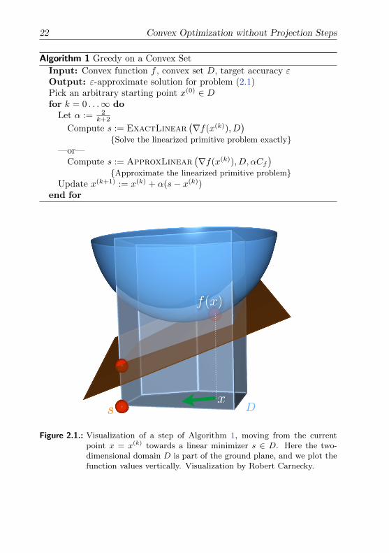
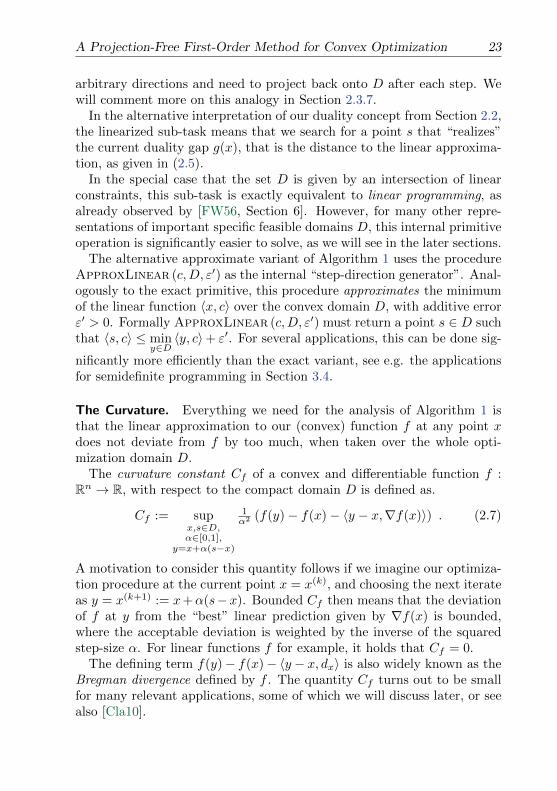
Algorithm 1 Greedy on a Convex Set
Input: Convex function f , convex set D, target accuracy εOutput: ε-approximate solution for problem (2.1)Pick an arbitrary starting point x(0) ∈ Dfor k = 0 . . .∞ do
Let α := 2k+2
Compute s := ExactLinear(∇f(x(k)), D
)Solve the linearized primitive problem exactly
—or—Compute s := ApproxLinear
(∇f(x(k)), D, αCf
)Approximate the linearized primitive problem
Update x(k+1) := x(k) + α(s− x(k))end for
xs D
f(x)
Figure 2.1.: Visualization of a step of Algorithm 1, moving from the currentpoint x = x(k) towards a linear minimizer s ∈ D. Here the two-dimensional domain D is part of the ground plane, and we plot thefunction values vertically. Visualization by Robert Carnecky.
A Projection-Free First-Order Method for Convex Optimization 23
arbitrary directions and need to project back onto D after each step. Wewill comment more on this analogy in Section 2.3.7.
In the alternative interpretation of our duality concept from Section 2.2,the linearized sub-task means that we search for a point s that “realizes”the current duality gap g(x), that is the distance to the linear approxima-tion, as given in (2.5).
In the special case that the set D is given by an intersection of linearconstraints, this sub-task is exactly equivalent to linear programming, asalready observed by [FW56, Section 6]. However, for many other repre-sentations of important specific feasible domains D, this internal primitiveoperation is significantly easier to solve, as we will see in the later sections.
The alternative approximate variant of Algorithm 1 uses the procedureApproxLinear (c,D, ε′) as the internal “step-direction generator”. Anal-ogously to the exact primitive, this procedure approximates the minimumof the linear function 〈x, c〉 over the convex domain D, with additive errorε′ > 0. Formally ApproxLinear (c,D, ε′) must return a point s ∈ D suchthat 〈s, c〉 ≤ min
y∈D〈y, c〉+ ε′. For several applications, this can be done sig-
nificantly more efficiently than the exact variant, see e.g. the applicationsfor semidefinite programming in Section 3.4.
The Curvature. Everything we need for the analysis of Algorithm 1 isthat the linear approximation to our (convex) function f at any point xdoes not deviate from f by too much, when taken over the whole opti-mization domain D.
The curvature constant Cf of a convex and differentiable function f :Rn → R, with respect to the compact domain D is defined as.
Cf := supx,s∈D,α∈[0,1],
y=x+α(s−x)
1α2 (f(y)− f(x)− 〈y − x,∇f(x)〉) . (2.7)
A motivation to consider this quantity follows if we imagine our optimiza-tion procedure at the current point x = x(k), and choosing the next iterateas y = x(k+1) := x+α(s−x). Bounded Cf then means that the deviationof f at y from the “best” linear prediction given by ∇f(x) is bounded,where the acceptable deviation is weighted by the inverse of the squaredstep-size α. For linear functions f for example, it holds that Cf = 0.
The defining term f(y)− f(x)− 〈y − x, dx〉 is also widely known as theBregman divergence defined by f . The quantity Cf turns out to be smallfor many relevant applications, some of which we will discuss later, or seealso [Cla10].
24 Convex Optimization without Projection Steps
The assumption of bounded curvature Cf is indeed very similar to aLipschitz assumption on the gradient of f , see also the discussion in Sec-tions 2.3.4 and 2.3.7. In the optimization literature, this property is some-times also called Cf -strong smoothness.
It will not always be possible to compute the constant Cf exactly. How-ever, for all algorithms in the following, and also their analysis, it is suf-ficient to just use some upper bound on Cf . We will comment in somemore details on the curvature measure in Section 2.3.4.
Convergence. The following theorem shows that after O(
1ε
)many it-
erations, Algorithm 1 obtains an ε-approximate solution. The analysisessentially follows the approach of [Cla10], inspired by the earlier workof [FW56, DH78, Pat93] and [Zha03]. Later, in Section 3.1.2, we will showthat this convergence rate is indeed best possible for this type of algorithm,when considering optimization over the unit-simplex. More precisely, wewill show that the dependence of the sparsity on the approximation qual-ity, as given by the algorithm here, is best possible up to a constant factor.Analogously, for the case of semidefinite optimization with bounded trace,we will prove in Section 3.4.4 that the obtained (low) rank of the approx-imations given by this algorithm is optimal, for the given approximationquality.
Theorem 2.3 (Primal Convergence). For each k ≥ 1, the iterate x(k) of theexact variant of Algorithm 1 satisfies
f(x(k))− f(x∗) ≤ 4Cfk + 2
,
where x∗ ∈ D is an optimal solution to problem (2.1). For the approximatevariant of Algorithm 1, it holds that
f(x(k))− f(x∗) ≤ 8Cfk + 2
.
(In other words both algorithm variants deliver a solution of primal errorat most ε after O( 1
ε ) many iterations.)
The proof of the above theorem on the convergence-rate of the primalerror crucially depends on the following Lemma 2.4 on the improvementin each iteration. We recall from Section 2.2 that the duality gap forthe general convex problem (2.1) over the domain D is given by g(x) =maxs∈D〈x− s,∇f(x)〉.
A Projection-Free First-Order Method for Convex Optimization 25
Lemma 2.4. For any step x(k+1) := x(k) +α(s− x(k)) with arbitrary step-size α ∈ [0, 1], it holds that
f(x(k+1)) ≤ f(x(k))− αg(x(k)) + α2Cf
if s is given by s := ExactLinear (∇f(x), D).If the approximate primitive s := ApproxLinear (∇f(x), D, αCf ) is
used instead, then it holds that
f(x(k+1)) ≤ f(x(k))− αg(x(k)) + 2α2Cf .
Proof. We write x := x(k), y := x(k+1) = x + α(s − x), and dx := ∇f(x)to simplify the notation, and first prove the second part of the lemma. Weuse the definition of the curvature constant Cf of our convex function f ,to obtain
f(y) = f(x+ α(s− x))≤ f(x) + α〈s− x, dx〉+ α2Cf .
Now we use that the choice of s := ApproxLinear (dx, D, ε′) is a good
“descent direction” on the linear approximation to f at x. Formally, weare given a point s that satisfies 〈s, dx〉 ≤ min
y∈D〈y, dx〉+ε′, or in other words
we have〈s− x, dx〉 ≤ miny∈D〈y, dx〉 − 〈x, dx〉+ ε′
= −g(x, dx) + ε′ ,
from the definition (2.5) of the duality gap g(x) = g(x, dx). Altogether,we obtain
f(y) ≤ f(x) + α(−g(x) + ε′) + α2Cf= f(x)− αg(x) + 2α2Cf ,
the last equality following by our choice of ε′ = αCf . This proves thelemma for the approximate case. The first claim for the exact linear prim-itive ExactLinear() follows by the same proof for ε′ = 0.
Having Lemma 2.4 at hand, the proof of our above primal convergenceTheorem 2.3 now follows along the same idea as in [Cla10, Theorem 2.3]or [Haz08, Theorem 1]. Note that a weaker variant of Lemma 2.4 wasalready proven by [FW56].
Proof of Theorem 2.3. From Lemma 2.4 we know that for every step of theexact variant of Algorithm 1, it holds that f(x(k+1)) ≤ f(x(k))−αg(x(k))+α2Cf .

26 Convex Optimization without Projection Steps
Writing h(x) := f(x) − f(x∗) for the (unknown) primal error at anypoint x, this implies that
h(x(k+1)) ≤ h(x(k))− αg(x(k)) + α2Cf≤ h(x(k))− αh(x(k)) + α2Cf= (1− α)h(x(k)) + α2Cf ,
(2.8)
where we have used weak duality h(x) ≤ g(x) as given by in (2.6). We willnow use induction over k in order to prove our claimed bound, i.e.,
h(x(k+1)) ≤ 4Cfk + 1 + 2
k = 0 . . .∞ .
The base-case k = 0 follows from (2.8) applied for the first step of thealgorithm, using α = α(0) = 2
0+2 = 1.Now considering k ≥ 1, the bound (2.8) gives us
h(x(k+1)) ≤ (1− α(k))h(x(k)) + α(k)2Cf
= (1− 2k+2 )h(x(k)) + ( 2
k+2 )2Cf
≤ (1− 2k+2 )
4Cfk+2 + ( 2
k+2 )2Cf ,
where in the last inequality we have used the induction hypothesis for x(k).Simply rearranging the terms gives
h(x(k+1)) ≤ 4Cfk+2 −
8Cf(k+2)2 +
4Cf(k+2)2
= 4Cf
(1k+2 − 1
(k+2)2
)=
4Cfk+2
k+2−1k+2
≤ 4Cfk+2
k+2k+3
=4Cfk+3 ,
which is our claimed bound for k ≥ 1.The analogous claim for Algorithm 1 using the approximate linear prim-
itive ApproxLinear() follows from the exactly same argument, by replac-ing every occurrence of Cf in the proof here by 2Cf instead (compare toLemma 2.4 also).
2.3.2. Obtaining a Guaranteed Small Duality Gap
From the above Theorem 2.3 on the convergence of Algorithm 1, we haveobtained small primal error. However, the optimum value f(x∗) is un-known in most practical applications, where we would prefer to have an
A Projection-Free First-Order Method for Convex Optimization 27
easily computable measure of the current approximation quality, for exam-ple as a stopping criterion of our optimizer in the case that Cf is unknown.The duality gap g(x) that we defined in Section 2.2 satisfies these require-ments, and always upper bounds the primal error f(x)− f(x∗).
By a nice argument of Clarkson [Cla10, Theorem 2.3], the convergenceon the simplex optimization domain can be extended to obtain the strongerproperty of guaranteed small duality gap g(x(k)) ≤ ε, after at most O( 1
ε )many iterations. This stronger convergence result was not yet known inearlier papers of [FW56, DH78, Jon92, Pat93] and [Zha03]. Here we willgeneralize the primal-dual convergence to arbitrary compact convex do-mains. The proof of our theorem below again relies on Lemma 2.4.
Theorem 2.5 (Primal-Dual Convergence). Let K :=⌈
4Cfε
⌉. We run the
exact variant of Algorithm 1 for K iterations (recall that the step-sizes aregiven by α(k) := 2
k+2 , 0 ≤ k ≤ K), and then continue for another K + 1
iterations, now with the fixed step-size α(k) := 2K+2 for K ≤ k ≤ 2K + 1.
Then the algorithm has an iterate x(k), K ≤ k ≤ 2K + 1, with dualitygap bounded by
g(x(k)) ≤ ε .The same statement holds for the approximate variant of Algorithm 1,
when setting K :=⌈
8Cfε
⌉instead.
Proof. The proof follows the idea of [Cla10, Section 7].By our previous Theorem 2.3 we already know that the primal error
satisfies h(x(K)) = f(x(K)) − f(x∗) ≤ 4CfK+2 after K iterations. In the
subsequent K+1 iterations, we will now suppose that g(x(k)) always stays
larger than4CfK+2 . We will try to derive a contradiction to this assumption.
Putting the assumption g(x(k)) >4CfK+2 into the step improvement bound
given by Lemma 2.4, we get that
f(x(k+1))− f(x(k)) ≤ −α(k)g(x(k)) + α(k)2Cf
< −α(k) 4CfK+2 + α(k)2
Cf
holds for any step size α(k) ∈ (0, 1]. Now using the fixed step-size α(k) =2
K+2 in the iterations k ≥ K of Algorithm 1, this reads as
f(x(k+1))− f(x(k)) < − 2K+2
4CfK+2 + 4
(K+2)2Cf
= − 4Cf(K+2)2
28 Convex Optimization without Projection Steps
Summing up over the additional steps, we obtain
f(x(2K+2))− f(x(K)) =2K+1∑k=K
f(x(k+1))− f(x(k))
< −(K + 2)4Cf
(K+2)2 = − 4CfK+2 ,
which together with our known primal approximation error f(x(K)) −f(x∗) ≤ 4Cf
K+2 would result in f(x(2K+2)) − f(x∗) < 0, a contradiction.
Therefore there must exist k, K ≤ k ≤ 2K + 1, with g(x(k)) ≤ 4CfK+2 ≤ ε.
The analysis for the approximate variant of Algorithm 1 follows usingthe analogous second bound from Lemma 2.4.
Following [Cla10, Theorem 2.3], one can also prove a similar primal-dual convergence theorem for the line-search algorithm variant that usesthe optimal step-size in each iteration, as we will discuss in the next Sec-tion 2.3.3. This is somewhat expected as the line-search algorithm in eachstep is at least as good as the fixed step-size variant we consider here.
2.3.3. Choosing the Optimal Step-Size by Line-Search
Alternatively, instead of the fixed step-size α = 2k+2 in Algorithm 1, one
can also find the optimal α ∈ [0, 1] by line-search. This will not improvethe theoretical convergence guarantee, but might still be considered inpractical applications if the best α is easy to compute. Experimentally, weobserved that line-search can improve the numerical stability in particularif approximate step directions are used, which we will discuss e.g. forsemidefinite matrix completion problems in Section 4.5.
Formally, given the chosen direction s, we then search for the α of bestimprovement in the objective function f , that is
α := arg minα∈[0,1]
f(x(k) + α(s− x(k))
). (2.9)
The resulting modified version of Algorithm 1 is depicted again in Algo-rithm 2, and was precisely analyzed in [Cla10] for the case of optimizingover the simplex.
In many cases, we can solve this line-search analytically in a straight-forward manner, by differentiating the above expression with respect to α:
Consider fα := f(x
(k+1)(α)
)= f
(x(k) + α
(s− x(k)
))and compute
0!=
∂
∂αfα =
⟨s− x(k),∇f
(x
(k+1)(α)
)⟩. (2.10)
A Projection-Free First-Order Method for Convex Optimization 29
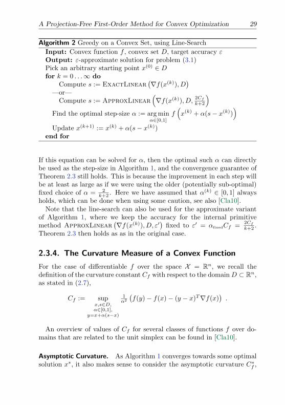
Algorithm 2 Greedy on a Convex Set, using Line-Search
Input: Convex function f , convex set D, target accuracy εOutput: ε-approximate solution for problem (3.1)Pick an arbitrary starting point x(0) ∈ Dfor k = 0 . . .∞ do
Compute s := ExactLinear(∇f(x(k)), D
)—or—
Compute s := ApproxLinear(∇f(x(k)), D,
2Cfk+2
)Find the optimal step-size α := arg min
α∈[0,1]
f(x(k) + α(s− x(k))
)Update x(k+1) := x(k) + α(s− x(k))
end for
If this equation can be solved for α, then the optimal such α can directlybe used as the step-size in Algorithm 1, and the convergence guarantee ofTheorem 2.3 still holds. This is because the improvement in each step willbe at least as large as if we were using the older (potentially sub-optimal)fixed choice of α = 2
k+2 . Here we have assumed that α(k) ∈ [0, 1] alwaysholds, which can be done when using some caution, see also [Cla10].
Note that the line-search can also be used for the approximate variantof Algorithm 1, where we keep the accuracy for the internal primitivemethod ApproxLinear
(∇f(x(k)), D, ε′
)fixed to ε′ = αfixedCf =
2Cfk+2 .
Theorem 2.3 then holds as as in the original case.
2.3.4. The Curvature Measure of a Convex Function
For the case of differentiable f over the space X = Rn, we recall thedefinition of the curvature constant Cf with respect to the domainD ⊂ Rn,as stated in (2.7),
Cf := supx,s∈D,α∈[0,1],
y=x+α(s−x)
1α2
(f(y)− f(x)− (y − x)T∇f(x)
).
An overview of values of Cf for several classes of functions f over do-mains that are related to the unit simplex can be found in [Cla10].
Asymptotic Curvature. As Algorithm 1 converges towards some optimalsolution x∗, it also makes sense to consider the asymptotic curvature C∗f ,
30 Convex Optimization without Projection Steps
defined as
C∗f := sups∈D,α∈[0,1],
y=x∗+α(s−x∗)
1α2
(f(y)− f(x∗)− (y − x∗)T∇f(x∗)
). (2.11)
Clearly C∗f ≤ Cf . As described in [Cla10, Section 4.4], we expect that asthe algorithm converges towards x∗, also the improvement bound as givenby Lemma 2.4 should be determined by C∗f + o(1) instead of Cf , resultingin a better convergence speed constant than given Theorem 2.3, at least forlarge k. The class of strongly convex functions is an example for which theconvergence of the relevant constant towards C∗f is easy to see, since forthese functions, convergence in the function value also imlies convergencein the domain, towards a unique point x∗, see e.g. [BV04, Section 9.1.2].
Relating the Curvature to the Hessian Matrix. Before we can comparethe assumption of bounded curvature Cf to a Lipschitz assumption on thegradient of f , we will need to relate Cf to the Hessian matrix (matrix ofall second derivatives) of f .
Here the idea described in [Cla10, Section 4.1] is to make use of thedegree-2 Taylor-expansion of our function f at the fixed point x, as afunction of α, which is
f(x+ α(s− x)) = f(x) + α(s− x)T∇f(x) +α2
2(s− x)T∇2f(z)(s− x) ,
where z is a point on the line-segment [x, y] ⊆ D ⊂ Rd between the twopoints x ∈ Rn and y = x+ α(s− x) ∈ Rn. To upper bound the curvaturemeasure, we can now directly plug in this expression for f(y) into theabove definition of Cf , obtaining
Cf ≤ supx,y∈D,
z∈[x,y]⊆D
1
2(y − x)T∇2f(z)(y − x) . (2.12)
From this bound, it follows that Cf is upper bounded by the largest eigen-value of the Hessian matrix of f , scaled with the domain’s Euclidean di-ameter, or formally
Lemma 2.6. For any twice differentiable convex function f over a compactconvex domain D, it holds that
Cf ≤1
2diam(D)2 · sup
z∈Dλmax
(∇2f(z)
).
A Projection-Free First-Order Method for Convex Optimization 31
Note that as f is convex, the Hessian matrix ∇2f(z) is positive semidef-inite for all z, see e.g. [KZ05, Theorem 7.3.6].
Proof. Applying the Cauchy-Schwarz inequality to (2.12) for any x, y ∈ D(as in the definition of Cf ), we get
(y − x)T∇2f(z)(y − x) ≤ ‖y − x‖2∥∥∇2f(z)(y − x)
∥∥2
≤ ‖y − x‖22∥∥∇2f(z)
∥∥spec
≤ diam(D)2 · supz∈D
λmax
(∇2f(z)
).
The middle inequality follows from the variational characterization of the
matrix spectral norm, i.e. ‖A‖spec := supx 6=0‖Ax‖2‖x‖2
. Finally, in the last
inequality we have used that by convexity of f , the Hessian matrix ∇2f(z)is PSD, so that its spectral norm is its largest eigenvalue.
Note that in the case of D being the unit simplex (see also the followingSection 3.1), we have that diam(∆n) =
√2, meaning the scaling factor
disappears, i.e. Cf ≤ supz∈∆n
λmax
(∇2f(z)
).
Bounded Curvature vs. Lipschitz-Continuous Gradient. Our core as-sumption on the given optimization problems is that that the curvatureCf of the function is bounded over the domain. Equivalently, this meansthat the function does not deviate from its linear approximation by toomuch. Here we will explain that this assumption is in fact very close to thenatural assumption that the gradient ∇f is Lipschitz-continuous, which isoften assumed in classical convex optimization literature, where it is some-times called Cf -strong smoothness, see e.g. [Nem05, KSST09] (or [d’A08]if the gradient information is only approximate).
Lemma 2.7. Let f be a convex and twice differentiable function, and as-sume that the gradient ∇f is Lipschitz-continuous over the domain D withLipschitz-constant L > 0. Then
Cf ≤1
2diam(D)2L .
Proof. Having ‖∇f(y)−∇f(x)‖2 ≤ L ‖y − x‖2 ∀x, y ∈ D by the Cauchy-
Schwarz inequality implies that (y − x)T (∇f(y) − ∇f(x)) ≤ L ‖y − x‖22,so that
f(y) ≤ f(x) + (y − x)T∇f(x) +L
2‖y − x‖22 . (2.13)
32 Convex Optimization without Projection Steps
If f is twice differentiable, it can directly be seen that the above con-dition implies that L · I ∇2f(z) holds for the Hessian of f , that isλmax
(∇2f(z)
)≤ L.
Together with our result from Lemma 2.6, the claim follows.
The above bound (2.13) which is implied by Lipschitz-continuous gra-dient means that the function is not “curved” by more than L in somesense, which is an interesting property. In fact this is exactly the oppositeinequality compared to the property of strong convexity, which is an as-sumption on the function f that we do not impose here. Strong convexityon a compact domain means that the function is always curved at least bysome constant (as our L). We just note that for strongly convex functions,“accelerated” algorithms with an even faster convergence of 1
k2 (meaningO( 1√
ε) steps) do exist [Nes04, Nes07a].
2.3.5. Optimizing over Convex Hulls
In the case that the optimization domain D is given as the convex hull ofa (finite or infinite) subset V ⊂ X , i.e.
D = conv(V ) ,
then it is particularly easy to solve the linear optimization subproblems asneeded in our Algorithm 1. Recall that conv(V ) is defined as the set ofall finite convex combinations
∑i αivi for a finite subset v1, . . . , vk ⊆ V ,
while V can also be an infinite set.
Lemma 2.8 (Linear Optimization over Convex Hulls). Let D = conv(V ) forany subset V ⊂ X , and D compact. Then any linear function y 7→ 〈y, c〉will attain its minimum and maximum over D at some “vertex” v ∈ V .
Proof. W.l.g. we will only show the case for the maximum. Let s ∈ Dbe a point attaining the linear optimum 〈s, c〉 = maxy∈D〈y, c〉. Then
by definition of D, we have that s =∑ki=1 αivi, meaning that s is the
weighted average of some finite set of “vertices” v1, . . . , vk ∈ V , with αi ≥0,∑i αi = 1. By linearity of the inner product,
〈s, c〉 =
⟨k∑i=1
αivi, c
⟩=
k∑i=1
αi〈vi, c〉 ,
and therefore we must have that 〈vi, c〉 ≥ 〈s, c〉 for at least one of theindices i, meaning that vi ∈ V is also attaining the linear maximum.
A Projection-Free First-Order Method for Convex Optimization 33
In the following we will discuss several application where this simplefact will be useful to solve the linearized subproblems ExactLinear()more efficiently, as the set V is often much easier to describe than the fullcompact domain D.
The setting of convex optimization over a convex hull in a vector spacewas already studied by [Zha03]. There, each iteration of the optimizerconsists of greedily selecting the point (or “vertex”) of V which promisesbest improvement. [Zha03] then gave a similar primal convergence guar-antee as in our Theorem 2.3 (but no primal-dual convergence result ongeneral convex hulls was known so far, to the best of our knowledge). Theabove Lemma 2.8 in a sense explains the relation to our linearized internalproblem. The main difference is that the algorithm of [Zha03] always eval-uates the original non-linear function f at all vertices V , while our slightlymore general framework only relies on the linear subproblem, and allowsfor arbitrary means to approximately solve the subproblem.
2.3.6. Randomized Variants, and Stochastic Optimization
For a variety of classes of our convex optimization problems, randomizationcan help to solve the linearized subproblem more efficiently. This idea isstrongly related to online and stochastic optimization, see e.g. [Nes11], andalso the popular stochastic gradient descent (SGD) techniques [Bot10].
We can also apply such cheaper randomized steps in our described frame-work, instead of deterministically solving the internal linear problem ineach iteration. Assumed that the user of our method is able to decomposethe linearized problem in some arbitrary way using randomization, and ifthe randomization is such that the linearized problem will be solved “ac-curately enough” with some probability p > 0 in each iteration, then ourconvergence analysis still holds also in this probabilistic setting as follows:
Formally, we assume that we are given access to a randomized pro-cedure RandomLinear (c,D, ε′), which returns a point s ∈ D such that〈s, c〉 ≤ min
y∈D〈y, c〉+ε′ with probability at least p > 0. In other words, with a
positive probability, RandomLinear() will behave like ApproxLinear().In each iteration of the line-search variant of our algorithm (see Algo-rithm 2), we will now use that randomized internal procedure instead. Theexpected improvement given by a step towards s = RandomLinear() isat least p times the amount given in Lemma 2.4. (Here we have used that inthe events of “failure” of RandomLinear(), the objective function valuewill at least not become worse, due to the use of line-search).
In other words if we perform 1p times more iterations than required
34 Convex Optimization without Projection Steps
for the deterministic Algorithm 1, then we have that the convergence byTheorem 2.3 also holds for the randomized variant described here.
Stochastic Gradient Descent (SGD). A classical example is when thelinearized problem is given by simply finding the maximum over say ncoordinates, as we will e.g. see in the following Sections 3.1 and 3.2 foroptimizing over the simplex, or over bounded `1-norm. In this case, bysampling uniformly at random, with probability 1
n we will pick the correctcoordinate, for which the step improvement is as in the deterministic Al-gorithm 1. Therefore we have obtained the same convergence guaranteeas for the deterministic algorithm, but the necessary number of steps ismultiplied by n.
For unconstrained convex optimization, the convergence of SGD andother related methods was analyzed e.g. in [Nes11] and also the earlier pa-per [Nes07b, Section 6]. Also here, a comparable slow-down was observedwhen using the cheaper randomized steps.
2.3.7. Relation to Classical Convex Optimization
Relation to Gradient Descent and Steepest Descent. The internal lin-ear optimizer in our Algorithm 1 can also be interpreted in terms of descentdirections. Recall that all vectors y that have negative scalar product withthe current gradient, i.e. 〈y,∇f(x)〉 < 0, are called descent directions, seee.g. [BV04, Chapter 9.4]. Also observe that 〈y,∇f(x)〉 is the directionalderivative of f in direction of y if y is of unit length. Our method there-fore chooses the best descent direction over the entire domain D, wherethe quality is measured as the best possible absolute improvement as sug-gested by the linearization at the current point x. In any iteration, thiswill crucially depend on the global shape of the domain D, even if theactual step-size α(k) might be very small.
This crucially contrasts classical gradient descent techniques, which onlyuse local information to determine the step-directions, facing the risk ofwalking out of the domain D and therefore requiring projection steps aftereach iteration.
Relation to Inaccurate and Missing Gradient Information. The abilityof our Algorithm 1 to deal with only approximate internal linear optimizersas in ApproxLinear() is also related to existing methods that assumethat gradient information is only available with noise, or in a stochastic orsampling setting.
A Projection-Free First-Order Method for Convex Optimization 35
For the case of optimizing smooth convex functions, [d’A08] has used asimilar measure of error, namely that the linearization given by the “noisy”version dx of the gradient ∇f(x) does not differ by more than say ε′ whenmeasured over the entire domain D, or formally∣∣∣〈y − z, dx〉 − 〈y − z,∇f(x)〉
∣∣∣ ≤ ε′ , ∀x, y, z ∈ D .
This assumption is similar, but stronger than the additive approximationquality that we require in our above setting (we only need that the lin-earized optimal values are within ε′). Also, the algorithm as well as theanalysis in [d’A08] are more complicated than the method proposed here,due to the need of projections and proximal operators.
We have discussed the case where gradient information is available onlyin a stochastic oracle (e.g. such that the gradient is obtained in expecta-tion) in the above Subsection 2.3.6. For an overview of related randomizedmethods in unconstrained convex optimization, we refer the reader to therecent work by [Nes11], which also applies when the gradient itself is notavailable and has to be estimated by oracle calls to the function alone.
If gradient information can be constructed in any way such that thelinearized problem ApproxLinear() can be solved to the desired additiveerror, then our above analysis of Algorithm 1 will still hold.
Relation to Mirror Descent, Proximal Methods and Conjugate Func-tions. Our proposed method is related to mirror descent as well as prox-imal methods in convex optimization, but our approach is usually simpler.The mirror descent technique originates from e.g. [BT03, BTN05]. Fora brief overview of proximal methods with applications to some of theclasses of sparse convex optimization problems as studied here, we referto [BJMO11, Section 3].
To investigate the connection, we write flin|x(y) := f(x) + 〈y−x, dx〉 forthe linearization given by the (sub)gradient dx = ∇f(x) at a fixed pointx ∈ D. A variant of mirror descent, see e.g. [BTN05, Haz11] is to find thenext iterate y as the point maximizing the Bregman divergence
f(y)− f(x)− 〈y − x, dx〉 = f(y)− flin|x(y) (2.14)
relative to the currently fixed old iterate x. This is the same task as maxi-mizing the gap between the function f(y) and its linear approximation at x,or equivalently we evaluate the conjugate function f∗(z) := sup
y∈D〈y, z〉−f(y)
at z = dx. The definition of the conjugate dual is also known as Fenchel
36 Convex Optimization without Projection Steps
duality, see e.g. [BL06]. In [Nem05], the conjugate function is also calledthe Legendre transformation.
However in our approach, the inner task ExactLinear(dx, D) as well asApproxLinear(dx, D, ε
′) is a simpler linear problem. Namely, we directlyminimize the linearization at the current point x, i.e. we maximize
− f(x)− 〈y − x, dx〉 = −flin|x(y) (2.15)
and then move towards an approximate maximizer y. In terms of Fenchelduality, this simpler linear problem is the evaluation of the conjugate dualof the characteristic function of our domain D, i.e.
1∗D(z) := supy∈X〈y, z〉 − 1D(y) ,
where this function is evaluated at the current subgradient z = dx. Thecharacteristic function 1D : X → R of a set D ⊆ X is defined as 1D(y) = 0for y ∈ D and 1D(y) =∞ otherwise.
Compared to our algorithm, mirror descent schemes require a “projec-tion” step in each iteration, sometimes also called the proximal or mirroroperator. This refers to minimizing the linearization plus a strongly con-vex prox-function that punishes the distance to the starting point. If thesquared Euclidean norm is used, the mirror operator corresponds to thestandard projection back onto the domain D. Our method uses no suchprox-function, and neither is the zero-function a strongly convex one, aswould be required for mirror descent to work. It is expected that the com-putational cost per iteration of our method will in most application casesbe lower compared to mirror descent schemes.
For convex optimization over the simplex, which we will study in moredetails in the following Section 3.1, [BT03] have proposed a mirror de-scent algorithm, obtaining a convergence of f(x(k))− f(x∗) ≤
√2 lnn L√
k.
This however is worse than the convergence of our methods as given byTheorem 2.3. Our convergence is independent of the dimension n, andgoes with 1
k instead of 1√k
. Also the earlier paper by [BTMN01] only ob-
tained a convergence of O(
1√k
)for the case of Lipschitz-continuous convex
functions over the simplex.The NERML optimizer by [BTN05] is a variant of mirror descent that
memorizes several past linearizations of the objective function, to improvethe available knowledge about the current function landscape. It is anopen research question if this idea could also help in our setting here, orfor stochastic gradient descent schemes [Bot10].
3Applications to Sparse and
Low Rank Approximation
3.1. Sparse Approximation over the Simplex
As a first application of the general optimization scheme from the previousChapter 2, we will now consider optimization problems defined over theunit simplex, or in other words the non-negative vectors of `1-norm equalto one. This will serve as a warm-up case before considering `1-normregularized problems in the next Section 3.2.
Our approach here will allow us to understand the best achievable spar-sity of approximate solutions, as a function of the approximation quality,as already shown by [Cla10].
In particular, we will show that our main Algorithm 1 on page 22 andits analysis do lead to Clarkson’s approach [Cla10] for optimizing over thesimplex. In this case, it was already known that sparsity O
(1ε
)can always
be achieved by applying Algorithm 1 to the simplex domain, see [Cla10].We will also show that this is indeed optimal, by providing an asymp-totically matching lower bound in Section 3.1.2. Also, our analysis holdseven if the linear subproblems are only solved approximately, and allowsarbitrary starting points, in contrast to [Cla10].
Having this efficient algorithm giving sparsity O(
1ε
)is in particularly at-
37
38 Applications to Sparse and Low Rank Approximation
tractive in view of the computational complexity of vector cardinality min-imization, which is known to be NP-hard, by a reduction to Exact-Cover,see [Nat95]. Vector cardinality minimization here refers to finding thesparsest vector that is an ε-approximation to some given convex minimiza-tion problem. Formally, finding the sparsest x that satisfies ‖Ax− b‖2 ≤ εfor given A, b and ε.
Set-Up. We suppose that a basis has been chosen in the space X , so thatwe can assume X = Rn with the standard inner product 〈x, y〉 = xT y. Herewe consider one special class of the general optimization problems (2.1),namely we optimize over non-negative vectors that sum up to one, that is
minimizex∈Rn
f(x)
s.t. ‖x‖1 = 1 ,x ≥ 0 .
(3.1)
In the following we write ∆n := x ∈ Rn |x ≥ 0, ‖x‖1 = 1 for the unitsimplex in Rn. As the objective function f is now defined over Rn, allsubgradients or gradients of f will also be represented by vectors in Rn inthe following.
Note that the alternative case of optimizing under an inequality con-straint ‖x‖1 ≤ 1 instead of ‖x‖1 = 1 can easily be reduced to the aboveform (3.1) by introducing a new “slack” variable. Formally, one uses vec-tors x = (x1, . . . , xn, xn+1) ∈ Rn+1 instead and optimizes the function
f(x) := f(x1, . . . , xn) over the simplex domain ‖x‖1 = 1, x ≥ 0.
Coresets. The coreset concept was originally introduced in computa-tional geometry by [BHPI02] and [APV02]. For point-set problems, thecoreset idea refers to identifying a very small subset (coreset) of the points,such that the solution just on the coreset is guaranteed to be a good ap-proximation to original problem, as we e.g. describe in Chapter 5. Herefor general convex optimization, the role of the coreset points is taken bythe non-zero coordinates of our sought vector x instead. The coreset sizethen corresponds to the sparsity of x.
Formally if there exists an ε-approximate solution x ∈ D ⊆ Rn to theconvex optimization problem (2.1), using only k many non-zero coordi-nates, then we say that the corresponding coordinates of x form an ε-coreset of size k for problem (2.1).
In other words, the following upper and lower bounds of O(
1ε
)on the
sparsity of approximations for problem (3.1) are indeed matching upper
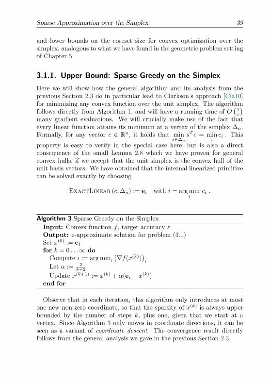
Sparse Approximation over the Simplex 39
and lower bounds on the coreset size for convex optimization over thesimplex, analogous to what we have found in the geometric problem settingof Chapter 5.
3.1.1. Upper Bound: Sparse Greedy on the Simplex
Here we will show how the general algorithm and its analysis from theprevious Section 2.3 do in particular lead to Clarkson’s approach [Cla10]for minimizing any convex function over the unit simplex. The algorithmfollows directly from Algorithm 1, and will have a running time of O
(1ε
)many gradient evaluations. We will crucially make use of the fact thatevery linear function attains its minimum at a vertex of the simplex ∆n.Formally, for any vector c ∈ Rn, it holds that min
s∈∆n
sT c = minici . This
property is easy to verify in the special case here, but is also a directconsequence of the small Lemma 2.8 which we have proven for generalconvex hulls, if we accept that the unit simplex is the convex hull of theunit basis vectors. We have obtained that the internal linearized primitivecan be solved exactly by choosing
ExactLinear (c,∆n) := ei with i = arg mini
ci .
Algorithm 3 Sparse Greedy on the Simplex
Input: Convex function f , target accuracy εOutput: ε-approximate solution for problem (3.1)Set x(0) := e1
for k = 0 . . .∞ doCompute i := arg mini
(∇f(x(k))
)i
Let α := 2k+2
Update x(k+1) := x(k) + α(ei − x(k))end for
Observe that in each iteration, this algorithm only introduces at mostone new non-zero coordinate, so that the sparsity of x(k) is always upperbounded by the number of steps k, plus one, given that we start at avertex. Since Algorithm 3 only moves in coordinate directions, it can beseen as a variant of coordinate descent. The convergence result directlyfollows from the general analysis we gave in the previous Section 2.3.
40 Applications to Sparse and Low Rank Approximation
Theorem 3.1 ([Cla10, Theorem 2.3], Convergence of Sparse Greedy on theSimplex). For each k ≥ 1, the iterate x(k) of Algorithm 3 satisfies
f(x(k))− f(x∗) ≤ 4Cfk + 2
.
where x∗ ∈ ∆n is an optimal solution to problem (3.1).
Furthermore, for any ε > 0, after at most 2⌈
4Cfε
⌉+ 1 = O
(1ε
)many
steps1, it has an iterate x(k) of sparsity O(
1ε
), satisfying g(x(k)) ≤ ε.
Proof. This is a corollary of Theorem 2.3 and Theorem 2.5.
Duality Gap. We recall from Section 2.2 that the duality gap (2.5) atany point x ∈ ∆n is easily computable from any subgradient, and in ourcase becomes
g(x, dx) = xT dx −mini
(dx)i , and
g(x) = xT∇f(x)−mini
(∇f(x))i .(3.2)
Here we have again used the observation that linear functions attain theirminimum at a vertex of the domain, i.e, min
s∈∆n
sT c = minici.
Applications. Many practically relevant optimization problems do fit intoour setting (3.1) here, allowing the application of Algorithm 3. This in-cludes linear classifiers such as support vector machines (SVMs), see alsoChapter 5, as well as kernel learning (finding the best convex combina-tion among a set of base kernels) [BLJ04]. Some other applications thatdirectly fit into our framework are `2-support vector regression (SVR),AdaBoost [Zha03], mean-variance analysis in portfolio selection [Mar52],the smallest enclosing ball problem [BC07], and estimating mixtures ofprobability densities [Cla10]. For more applications we refer to [Cla10].
Line-Search for the Best Step-Size. In most applications it will be astraight-forward task to find the optimal step-size α ∈ [0, 1] in each stepinstead, as described in Section 2.3.3.
1Note that in order for our Theorem 2.5 on the bounded duality gap to apply, thestep-size in the second half of the iterations needs to be fixed to α(k) := 2
K+2,
see Section 2.3.2. This remark also applies to the later applications of our generalAlgorithm 1 in this chapter. We already mentioned above that if line-search is usedinstead, then no such technicality is necessary, see also [Cla10].
Sparse Approximation over the Simplex 41
For the special case of polytope distance and SVM problems, the result-ing method then exactly corresponds to Gilbert’s geometric algorithm [Gil66],which we will study in Chapter 5. Here the wording of “line-search” makesgeometric sense in that we need to find the point s on a given line, suchthat s is closest to the origin.
Away Steps. By performing more work with the currently non-zero coor-dinates, one can get the sparsity even smaller. More precisely the number
of non-zeros can be improved close to2Cfε instead of 2
⌈4Cfε
⌉as given by
the above Theorem 3.1. The idea of away-steps introduced by [TY07] is tokeep the total number of non-zero coordinates (i.e. the coreset size) fixedover all iterations, by removing the smallest non-zero coordinate from xafter each adding step. We will discuss this idea for the geometric formu-lation of coresets in Chapter 5. For more background we refer to [Cla10,Algorithm 9.1].
3.1.2. Ω(1ε) Lower Bound on the Sparsity
We will now show that sparsity O(
1ε
), as obtained by the greedy algorithm
we analyzed in the previous section is indeed best possible, by providinga lower bound of Ω
(1ε
). In the language of coresets, this means we will
provide a matching lower bound on the size of coresets for convex opti-mization over the simplex. Together with the upper bound, this thereforecompletely characterizes the trade-off between sparsity and approxima-tion quality for the family of optimization problems of the form (3.1).The same matching sparsity upper and lower bounds will also hold foroptimizing over the `1-ball instead, see Section 3.2.
For the following lower bound construction we consider the differentiablefunction f(x) := ‖x‖22 = xTx. This function has gradient ∇f(x) = 2x.Its curvature constant is Cf = 2, which follows directly from the defini-tion (2.7), and the fact that here f(y)−f(x)−(y−x)T∇f(x) = yT y−xTx−(y−x)T 2x = ‖x− y‖22, so that Cf = supx,s∈∆n
‖x− s‖22 = diam(∆n)2 = 2.
The following lemmata show that the sparse greedy algorithm of [Cla10]from Section 3.1.1 is indeed optimal for the approximation quality (primalas well as dual error respectively), giving best possible sparsity, up to asmall multiplicative constant.
42 Applications to Sparse and Low Rank Approximation
Lemma 3.2. For f(x) := ‖x‖22, and 1 ≤ k ≤ n, it holds that
minx∈∆n
card(x)≤k
f(x) =1
k.
Proof. We prove the inequality minx..
f(x) ≥ 1k by induction on k.
Case k = 1 For any unit length vector x ∈ ∆n having just a singlenon-zero entry, f(x) = ‖x‖2 = ‖x‖1 = 1.
Case k > 1 For every x ∈ ∆n of sparsity card(x) ≤ k, we can pick acoordinate i with xi 6= 0, and write x = (1− α)v + αei as the sum of twoorthogonal vectors v and a unit basis vector ei, where v ∈ ∆n of sparsity≤ k − 1, vi = 0, and α = xi. So for every x ∈ ∆n of sparsity ≤ k, wetherefore get that
f(x) = ‖x‖22 = xTx= ((1− α)v + αei)
T ((1− α)v + αei)= (1− α)2vT v + α2
≥ (1− α)2 1k−1 + α2
≥ min0≤β≤1(1− β)2 1k−1 + β2
= 1k .
In the first inequality we have applied the induction hypothesis for v ∈ ∆n
of sparsity ≤ k − 1.Equality: The function value f(x) = 1
k is obtained by setting k of thecoordinates of x to 1
k each.
In other words for any vector x of sparsity card(x) = k, the primal errorf(x)− f(x∗) is always lower bounded by 1
k − 1n . For the duality gap g(x),
the lower bound is even slightly higher:
Lemma 3.3. For f(x) := ‖x‖22, and any k ∈ N, k < n, it holds that
g(x) ≥ 2
k∀x ∈ ∆n s.t. card(x) ≤ k.
Proof. g(x) = xT∇f(x) − mini(∇f(x))i = 2(xTx − mini xi). We nowuse mini xi = 0 because card(x) < n, and that by Lemma 3.2 we havexTx = f(x) ≥ 1
k .
Note: We could also consider the function f(x) := γ ‖x‖22 instead, forsome γ > 0. This f has curvature constant Cf = 2γ, and for this scaling,
our above lower bound on the duality gap will also scale linearly, givingCfk .
Sparse Approximation with Bounded `1-Norm 43
3.2. Sparse Approximation with Bounded`1-Norm
In this second application case, will apply the general greedy approachfrom Section 2.3 in order to understand the best achievable sparsity forconvex optimization under bounded `1-norm, as a function of the approxi-mation quality. Here the situation is indeed extremely similar to the aboveSection 3.1 of optimizing over the simplex, and the resulting algorithm willagain have a running time of O
(1ε
)many gradient evaluations.
It is known that the vector ‖.‖1-norm is the best convex approximationto the sparsity (cardinality) of a vector, that is card(.). More precisely,the function ‖.‖1 is the convex envelope of the sparsity, meaning that it isthe “largest” convex function that is upper bounded by the sparsity on theconvex domain of vectors x | ‖x‖∞ ≤ 1. This can be seen by observing
that card(x) ≥ ‖x‖1‖x‖∞
, see e.g. [RFP10]. We will discuss the analogous
generalization to matrices in Chapter 4, namely using the matrix nuclearnorm as the “best” convex approximation of the matrix rank.
Set-Up. Here we consider one special class of the general optimizationproblem (2.1), namely problems over vectors in Rn with bounded ‖.‖1-norm, that is
minimizex∈Rn
f(x)
s.t. ‖x‖1 ≤ 1 .(3.3)
We write ♦n := x ∈ Rn | ‖x‖1 ≤ 1 for the `1-ball in Rn. Note thatone can simply rescale the function argument to allow for more generalconstraints ‖x‖1 ≤ t for t > 0. Again we have X = Rn with the standardinner product 〈x, y〉 = xT y, so that also the subgradients or gradients off are represented as vectors in Rn.
The Linearized Problem. As already in the simplex case, the subprob-lem of optimizing a linear function over the `1-ball is particularly easy tosolve, allowing us to provide a fast implementation of the internal primitiveprocedure ExactLinear (c,♦n).
Namely, it is again easy to see that every linear function attains its mini-mum/maximum at a vertex of the ball ♦n, as we have already seen for gen-eral convex hulls in our earlier Lemma 2.8, and ♦n = conv(±ei | i ∈ [n]).Here this crucial observation can also alternatively be interpreted as theknown fact that the dual norm to the `1-norm is in fact the `∞-norm, seealso our earlier Observation 2.2.
44 Applications to Sparse and Low Rank Approximation
Observation 3.4. For any vector c ∈ Rn, it holds that
ei · sign(ci) ∈ arg maxy∈♦n
yT c
where i ∈ [n] is an index of a maximal coordinate of c measured in absolutevalue, or formally i ∈ arg maxj |cj |.
Using this observation for c = −∇f(x) in our general Algorithm 1, wetherefore directly obtain the following simple method for `1-regularizedconvex optimization, as depicted in the Algorithm 4.
Algorithm 4 Sparse Greedy on the `1-Ball
Input: Convex function f , target accuracy εOutput: ε-approximate solution for problem (3.3)Set x(0) := 0for k = 0 . . .∞ do
Compute i := arg maxi∣∣(∇f(x(k))
)i
∣∣,and let s := ei · sign
((−∇f(x(k))
)i
)Let α := 2
k+2
Update x(k+1) := x(k) + α(s− x(k))end for
Observe that in each iteration, this algorithm only introduces at mostone new non-zero coordinate, so that the sparsity of x(k) is always upperbounded by the number of steps k. This means that the method is againof coordinate-descent-type, as in the simplex case of the previous Sec-tion 3.1.1. Its convergence analysis again directly follows from the generalanalysis from Section 2.3.
Theorem 3.5 (Convergence of Sparse Greedy on the `1-Ball). For each k ≥ 1,the iterate x(k) of Algorithm 4 satisfies
f(x(k))− f(x∗) ≤ 4Cfk + 2
.
where x∗ ∈ ♦n is an optimal solution to problem (3.3).
Furthermore, for any ε > 0, after at most 2⌈
4Cfε
⌉+ 1 = O
(1ε
)many
steps, it has an iterate x(k) of sparsity O(
1ε
), satisfying g(x(k)) ≤ ε.
Proof. This is a corollary of Theorem 2.3 and Theorem 2.5.
Sparse Approximation with Bounded `1-Norm 45
The Duality Gap, and Duality of the Norms. We recall the definitionof the duality gap (2.5) given by the linearization at any point x ∈ ♦n,see Section 2.2. Thanks to our Observation 2.2, the computation of theduality gap in the case of the `1-ball here becomes extremely simple, andis given by the norm that is dual to the `1-norm, namely the `∞-norm ofthe used subgradient, i.e.,
g(x, dx) = ‖dx‖∞ + xT dx, and
g(x) = ‖∇f(x)‖∞ + xT∇f(x) .
Alternatively, the same expression can also be derived directly (withoutexplicitly using duality of norms) by applying the Observation 3.4.
A Lower Bound on the Sparsity. The lower bound of Ω(
1ε
)on the spar-
sity as proved in Section 3.1.2 for the simplex case in fact directly translatesto the `1-ball as well. Instead of choosing the objective function f as thedistance to the origin (which is part of the `1-ball), we consider the opti-
mization problem min‖x‖1≤1
f(x) := ‖x− r‖22 with respect to the fixed point
r := ( 2n , . . . ,
2n ) ∈ Rn. This problem is of the form (3.3), and corresponds
to optimizing the Euclidean distance to the point r given by mirroring theorigin at the positive facet of the `1-ball. Here by the “positive facet”, wemean the hyperplane defined by the intersection of the boundary of the`1-ball with the positive orthant, which is exactly the unit simplex. There-fore, the proof for the simplex case from Section 3.1.2 holds analogouslyfor our setting here.
We have thus obtained that sparsity O(
1ε
)as obtained by the greedy Al-
gorithm 4 is indeed best possible for `1-regularized optimization problemsof the form (3.3).
Using Barycentric Coordinates Instead. Clarkson [Cla10, Theorem 4.2]already observed that Algorithm 3 over the simplex ∆n can be used tooptimize a convex function f(y) over arbitrary convex hulls, by just usingbarycentric coordinates y = Ax, x ∈ ∆n, for A ∈ Rn×m being the ma-trix containing all m vertices of the convex domain as its columns. Herehowever we saw that for the `1-ball, the steps of the algorithm are evenslightly simpler, as well as that the duality gap can be computed instantlyfrom the `∞-norm of the gradient.
Applications. Our Algorithm 4 applies to arbitrary convex vector opti-mization problems with an ‖.‖1-norm regularization term, giving a guar-
46 Applications to Sparse and Low Rank Approximation
anteed sparsity of O(
1ε
)for all these applications.
A classical example for problems of this class is given by the impor-tant ‖.‖1-regularized least squares regression approach, which we alreadydiscussed in our introductory Section 1.3.1. Formally,
minx∈Rn
‖Ax− b‖22 + µ ‖x‖1
for a fixed matrix A ∈ Rm×n, a vector b ∈ Rm and a fixed regularizationparameter µ > 0. The same problem is also known as basis pursuit de-noising in the compressed sensing literature, which we will discuss moreprecisely in Section 3.2.1. The above formulation is in fact the Lagrangianformulation of the corresponding constrained problem for ‖x‖1 ≤ t forsome fixed parameter t corresponding to µ, see also Section 1.3.2. Thisequivalent formulation is also known as the Lasso problem [Tib96] whichis
minx∈Rn
‖Ax− b‖22s.t. ‖x‖1 ≤ t .
The above formulation is exactly a problem of our above form (3.3), namely
minx∈♦n
‖tAx− b‖22 ,
if we rescale the argument x =: tx so that ‖x‖1 ≤ 1.
Another important application for our result is logistic regression with‖.‖1-norm regularization, see e.g. [KKB07], which is also a convex opti-mization problem [Ren05]. The reduction to an `1-problem of our form (3.3)works exactly the same way as described here.
Related Work. As we mentioned above, the optimization problem (3.3)— if f is the squared error of a linear function — is very well studied as theLasso approach, see e.g. [Tib96] and the references therein. For generalobjective functions f of bounded curvature, the above interesting trade-offbetween sparsity and the approximation quality was already investigatedby [SSSZ10], and also by our earlier paper [GJ09] (see also Chapter 5) forthe analogous case of optimizing over the simplex. [SSSZ10, Theorem 2.4]shows a sparse convergence analogous to our above Theorem 3.5, for the“forward greedy selection” algorithm on problem (3.3), but only for thecase that f is differentiable.
Sparse Approximation with Bounded `1-Norm 47
3.2.1. Relation to Matching Pursuit and Basis Pursuit inCompressed Sensing
Both our sparse greedy Algorithm 3 for optimizing over the simplex andalso Algorithm 4 for general `1-problems are very similar to the techniqueof matching pursuit, which is one of the most popular techniques in sparserecovery in the vector case [Tro04].
Suppose we want to recover a sparse signal vector x ∈ Rn from anoisy measurement vector Ax = y ∈ Rm. For a given dictionary matrixA ∈ Rm×n, matching pursuit iteratively chooses the dictionary elementAi ∈ Rm that has the highest inner product with the current residual,and therefore reduces the representation error f(x) = ‖Ax− y‖22 by thelargest amount. This choice of coordinate i = arg maxj A
Tj (Ax−y) exactly
corresponds2 to the choice of i := arg minj(∇f(x(k))
)j
in Algorithm 3.
Another variant of matching pursuit, called orthogonal matching pur-suit (OMP) [Tro04, TG07], includes an extra orthogonalization step, andis closer related to the coreset algorithms that optimize over the all exist-ing set of non-zero coordinates before adding a new one, see e.g. [Cla10,Algorithm 8.2], or the analogous “fully corrective” variant of [SSSZ10]. Ify = Ax, with x sparse and the columns of A sufficiently incoherent, thenOMP recovers the sparsest representation for the given y [Tro04].
The paper [Zha11] recently proposed another algorithm that generalizesOMP, comes with a guarantee on correct sparse recovery, and also corre-sponds to “completely optimize within each coreset”. The method uses
the same choice of the new coordinate i := arg maxj
∣∣∣(∇f(x(k)))j
∣∣∣ as in
our Algorithm 4. However the analysis of [Zha11] requires the not onlybounded curvature as in our case, but also needs strong convexity of theobjective function (which then also appears as a multiplicative factor inthe number of iterations needed). Our Algorithm 4 as well as the earliermethod by [Zha03] are simpler to implement, and have a lower complexityper iteration, as we do not need to optimize over several currently non-zero coordinates, but only change one coordinate by a fixed amount ineach iteration.
Our Algorithm 4 for general `1-regularized problems also applies to solv-ing the so called basis pursuit problem [CDS98, FNW07] and [BV04, Sec-tion 6.5.4], which is minx∈Rn ‖x‖1 s.t. Ax = y. Note that this is in factjust the constrained variant of the corresponding “robust” `1-regularized
2The objective function f(x) := ‖Ax− y‖22 can be written as f(x) = (Ax− y)T (Ax−y) = xTATAx − 2yTAx − yT y, so its gradient is ∇f(x) = 2ATAx − 2AT y =2AT (Ax− y) ∈ Rn.
48 Applications to Sparse and Low Rank Approximation
least squares regression problem
minx∈Rn
‖Ax− y‖22 + µ ‖x‖1 ,
which is the equivalent trade-off variant of our problem of the form (3.3).[FNW07] propose a traditional gradient descent technique for solving theabove least squares problem, but do not give a convergence analysis.
We will discuss solution path algorithms with approximation guaranteesfor this problem (obtaining solutions for all values of the tradeoff param-eter µ) in Chapter 6.
3.3. Optimization with Bounded `∞-Norm
Applying our above general optimization framework for the special case ofthe domain being the ‖.‖∞-norm unit ball, we again obtain a very simplegreedy algorithm. The running time will again correspond to O
(1ε
)many
gradient evaluations. Formally, we consider problems of the form
minimizex∈Rn
f(x)
s.t. ‖x‖∞ ≤ 1 .(3.4)
We denote the feasible set, i.e. the ‖.‖∞-norm unit ball, by n :=x ∈ Rn | ‖x‖∞ ≤ 1. For this set, it will again be very simple to imple-ment the internal primitive operation of optimizing a linear function overthe same domain. The following crucial observation allows us to implementExactLinear (c,n) in a very simple way. This can also alternatively beinterpreted as the known fact that the dual-norm to the `∞-norm is the`1-norm, which also explains why the greedy algorithm we will obtain hereis very similar to the `1-version from the previous Section 3.2.
Observation 3.6. For any vector c ∈ Rn, it holds that
sc ∈ arg maxy∈n
yT c
where sc ∈ Rn is the sign-vector of c, defined by the sign of each individualcoordinate, i.e. (sc)i = sign(ci) ∈ −1, 1.
Using this observation for c = −dx in our general Algorithm 1, wedirectly obtain the following simple method for optimization over a box-domain n, as depicted in Algorithm 5.
The convergence analysis again directly follows from the general analysisfrom Section 2.3.
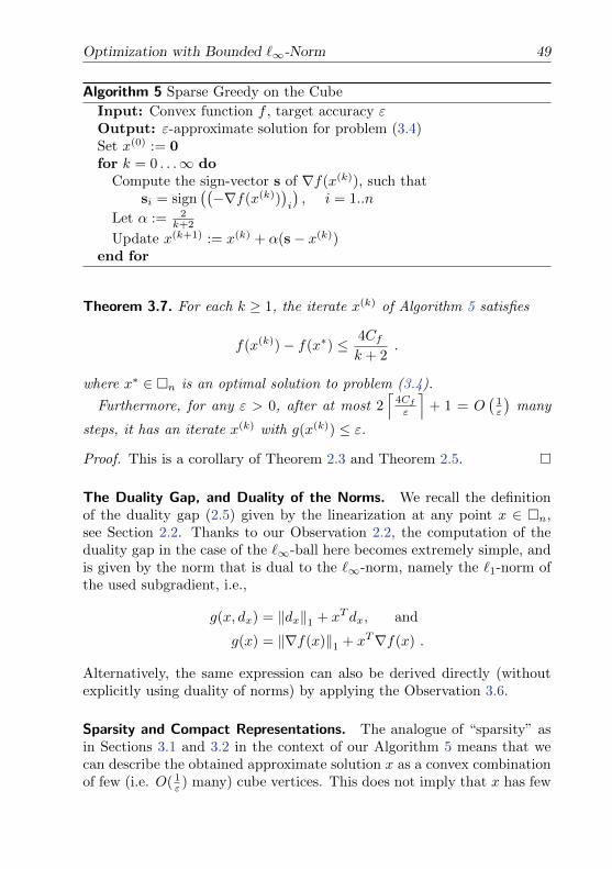
Optimization with Bounded `∞-Norm 49
Algorithm 5 Sparse Greedy on the Cube
Input: Convex function f , target accuracy εOutput: ε-approximate solution for problem (3.4)Set x(0) := 0for k = 0 . . .∞ do
Compute the sign-vector s of ∇f(x(k)), such thatsi = sign
((−∇f(x(k))
)i
), i = 1..n
Let α := 2k+2
Update x(k+1) := x(k) + α(s− x(k))end for
Theorem 3.7. For each k ≥ 1, the iterate x(k) of Algorithm 5 satisfies
f(x(k))− f(x∗) ≤ 4Cfk + 2
.
where x∗ ∈ n is an optimal solution to problem (3.4).
Furthermore, for any ε > 0, after at most 2⌈
4Cfε
⌉+ 1 = O
(1ε
)many
steps, it has an iterate x(k) with g(x(k)) ≤ ε.
Proof. This is a corollary of Theorem 2.3 and Theorem 2.5.
The Duality Gap, and Duality of the Norms. We recall the definitionof the duality gap (2.5) given by the linearization at any point x ∈ n,see Section 2.2. Thanks to our Observation 2.2, the computation of theduality gap in the case of the `∞-ball here becomes extremely simple, andis given by the norm that is dual to the `∞-norm, namely the `1-norm ofthe used subgradient, i.e.,
g(x, dx) = ‖dx‖1 + xT dx, and
g(x) = ‖∇f(x)‖1 + xT∇f(x) .
Alternatively, the same expression can also be derived directly (withoutexplicitly using duality of norms) by applying the Observation 3.6.
Sparsity and Compact Representations. The analogue of “sparsity” asin Sections 3.1 and 3.2 in the context of our Algorithm 5 means that wecan describe the obtained approximate solution x as a convex combinationof few (i.e. O( 1
ε ) many) cube vertices. This does not imply that x has few
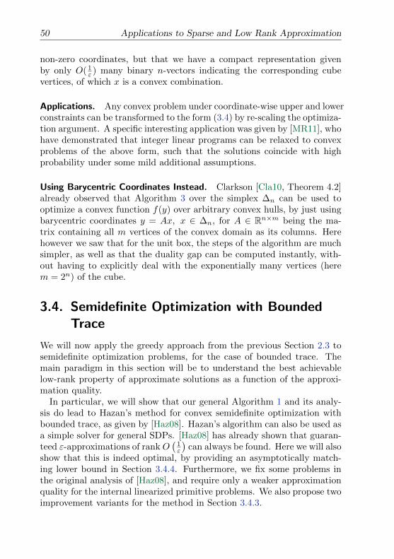
50 Applications to Sparse and Low Rank Approximation
non-zero coordinates, but that we have a compact representation givenby only O( 1
ε ) many binary n-vectors indicating the corresponding cubevertices, of which x is a convex combination.
Applications. Any convex problem under coordinate-wise upper and lowerconstraints can be transformed to the form (3.4) by re-scaling the optimiza-tion argument. A specific interesting application was given by [MR11], whohave demonstrated that integer linear programs can be relaxed to convexproblems of the above form, such that the solutions coincide with highprobability under some mild additional assumptions.
Using Barycentric Coordinates Instead. Clarkson [Cla10, Theorem 4.2]already observed that Algorithm 3 over the simplex ∆n can be used tooptimize a convex function f(y) over arbitrary convex hulls, by just usingbarycentric coordinates y = Ax, x ∈ ∆n, for A ∈ Rn×m being the ma-trix containing all m vertices of the convex domain as its columns. Herehowever we saw that for the unit box, the steps of the algorithm are muchsimpler, as well as that the duality gap can be computed instantly, with-out having to explicitly deal with the exponentially many vertices (herem = 2n) of the cube.
3.4. Semidefinite Optimization with BoundedTrace
We will now apply the greedy approach from the previous Section 2.3 tosemidefinite optimization problems, for the case of bounded trace. Themain paradigm in this section will be to understand the best achievablelow-rank property of approximate solutions as a function of the approxi-mation quality.
In particular, we will show that our general Algorithm 1 and its analy-sis do lead to Hazan’s method for convex semidefinite optimization withbounded trace, as given by [Haz08]. Hazan’s algorithm can also be used asa simple solver for general SDPs. [Haz08] has already shown that guaran-teed ε-approximations of rank O
(1ε
)can always be found. Here we will also
show that this is indeed optimal, by providing an asymptotically match-ing lower bound in Section 3.4.4. Furthermore, we fix some problems inthe original analysis of [Haz08], and require only a weaker approximationquality for the internal linearized primitive problems. We also propose twoimprovement variants for the method in Section 3.4.3.
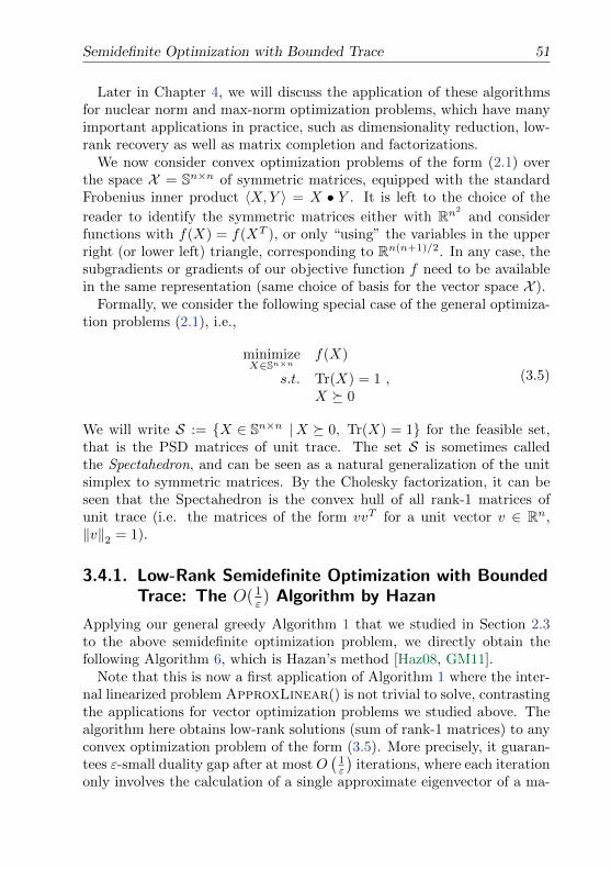
Semidefinite Optimization with Bounded Trace 51
Later in Chapter 4, we will discuss the application of these algorithmsfor nuclear norm and max-norm optimization problems, which have manyimportant applications in practice, such as dimensionality reduction, low-rank recovery as well as matrix completion and factorizations.
We now consider convex optimization problems of the form (2.1) overthe space X = Sn×n of symmetric matrices, equipped with the standardFrobenius inner product 〈X,Y 〉 = X • Y . It is left to the choice of the
reader to identify the symmetric matrices either with Rn2
and considerfunctions with f(X) = f(XT ), or only “using” the variables in the upperright (or lower left) triangle, corresponding to Rn(n+1)/2. In any case, thesubgradients or gradients of our objective function f need to be availablein the same representation (same choice of basis for the vector space X ).
Formally, we consider the following special case of the general optimiza-tion problems (2.1), i.e.,
minimizeX∈Sn×n
f(X)
s.t. Tr(X) = 1 ,X 0
(3.5)
We will write S := X ∈ Sn×n |X 0, Tr(X) = 1 for the feasible set,that is the PSD matrices of unit trace. The set S is sometimes calledthe Spectahedron, and can be seen as a natural generalization of the unitsimplex to symmetric matrices. By the Cholesky factorization, it can beseen that the Spectahedron is the convex hull of all rank-1 matrices ofunit trace (i.e. the matrices of the form vvT for a unit vector v ∈ Rn,‖v‖2 = 1).
3.4.1. Low-Rank Semidefinite Optimization with BoundedTrace: The O(1
ε) Algorithm by Hazan
Applying our general greedy Algorithm 1 that we studied in Section 2.3to the above semidefinite optimization problem, we directly obtain thefollowing Algorithm 6, which is Hazan’s method [Haz08, GM11].
Note that this is now a first application of Algorithm 1 where the inter-nal linearized problem ApproxLinear() is not trivial to solve, contrastingthe applications for vector optimization problems we studied above. Thealgorithm here obtains low-rank solutions (sum of rank-1 matrices) to anyconvex optimization problem of the form (3.5). More precisely, it guaran-tees ε-small duality gap after at most O
(1ε
)iterations, where each iteration
only involves the calculation of a single approximate eigenvector of a ma-
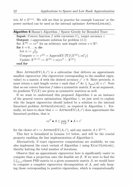
52 Applications to Sparse and Low Rank Approximation
trix M ∈ Sn×n. We will see that in practice for example Lanczos’ or thepower method can be used as the internal optimizer ApproxLinear().
Algorithm 6 Hazan’s Algorithm / Sparse Greedy for Bounded Trace
Input: Convex function f with curvature Cf , target accuracy εOutput: ε-approximate solution for problem (3.5)Set X(0) := vvT for an arbitrary unit length vector v ∈ Rn.for k = 0 . . .∞ do
Let α := 2k+2
Compute v := v(k) = ApproxEV(∇f(X(k)), αCf
)Update X(k+1) := X(k) + α(vvT −X(k))
end for
Here ApproxEV(A, ε′) is a subroutine that delivers an approximatesmallest eigenvector (the eigenvector corresponding to the smallest eigen-value) to a matrix A with the desired accuracy ε′ > 0. More precisely, itmust return a unit length vector v such that vTAv ≤ λmin(A) + ε′. Notethat as our convex function f takes a symmetric matrix X as an argument,its gradients ∇f(X) are given as symmetric matrices as well.
If we want to understand this proposed Algorithm 6 as an instanceof the general convex optimization Algorithm 1, we just need to explainwhy the largest eigenvector should indeed be a solution to the internallinearized problem ApproxLinear(), as required in Algorithm 1. For-mally, we have to show that v := ApproxEV(A, ε′) does approximate thelinearized problem, that is
vvT •A ≤ minY ∈S
Y •A+ ε′
for the choice of v := ApproxEV(A, ε′), and any matrix A ∈ Sn×n.
This fact is formalized in Lemma 3.8 below, and will be the crucialproperty enabling the fast implementation of Algorithm 6.
Alternatively, if exact eigenvector computations are available, we canalso implement the exact variant of Algorithm 1 using ExactLinear(),thereby halving the total number of iterations.
Observe that an approximate eigenvector here is significantly easier tocompute than a projection onto the feasible set S. If we were to find the‖.‖Fro-closest PSD matrix to a given symmetric matrix A, we would haveto compute a complete eigenvector decomposition of A, and only keep-ing those corresponding to positive eigenvalues, which is computationally
Semidefinite Optimization with Bounded Trace 53
expensive. By contrast, a single approximate smallest eigenvector com-putation as in ApproxEV(A, ε′) can be done in near linear time in thenumber of non-zero entries of A. We will discuss the implementation ofApproxEV(A, ε′) in more detail further below.
Sparsity becomes Low Rank. As the rank-1 matrices are indeed the“vertices” of the domain S as shown in Lemma 3.8 below, our Algorithm 6can be therefore seen as a matrix generalization of the sparse greedy ap-proximation algorithm of [Cla10] for vectors in the unit simplex, see Sec-tion 3.1, which has seen many successful applications. Here sparsity justgets replaced by low rank. By the analysis of the general algorithm inTheorem 2.3, we already know that we obtain ε-approximate solutions forany convex optimization problem (3.5) over the spectahedron S. Becauseeach iterate X(k) is represented as a sum (convex combination) of k manyrank-1 matrices vvT , it follows that X(k) is of rank at most k. Therefore,the resulting ε-approximations are of low rank, i.e. rank O
(1ε
).
For large-scale applications where 1ε n, the representation of X(k) as a
sum of rank-1 matrices is much more efficient than storing an entire matrixX(k) ∈ Sn×n. Later in Section 4.5 (or see also [JS10]) we will demonstratethat Algorithm 6 can readily be applied to practical problems for n ≥ 106
on an ordinary computer, well exceeding the possibilities of interior pointmethods.
[Haz08] already observed that the same Algorithm 6 with a well-craftedfunction f can also be used to approximately solve arbitrary SDPs withbounded trace, which we will briefly explain in Section 3.4.2.
Linearization, the Duality Gap, and Duality of the Norms. Here we willprove that the general duality gap (2.5) can be calculated very efficientlyfor the domain being the spectahedron S. From the following Lemma 3.8,we obtain that
g(X) =X • ∇f(X) + λmax(−∇f(X))
=X • ∇f(X)− λmin(∇f(X)) .(3.6)
As predicted by our Observation 2.2 on formulating the duality gap, wehave again obtained the dual norm to the norm that determines the domainD. It can be seen that over the space of symmetric matrices, the dual normof the matrix trace-norm (also known as the nuclear norm) is given by thespectral norm, i.e. the largest eigenvalue. To see this, we refer the readerto the later Section 4.2 on the properties of the nuclear norm and its dualcharacterization.
54 Applications to Sparse and Low Rank Approximation
The following Lemma 3.8 shows that any linear function attains itsminimum and maximum at a “vertex” of the Spectahedron S, as we havealready proved for the case of general convex hulls in Lemma 2.8.
Lemma 3.8. The spectahedron is the convex hull of the rank-1 matrices,
S = conv(vvT
∣∣ v ∈ Rn, ‖v‖2 = 1
) .
Furthermore, for any symmetric matrix A ∈ Sn×n, it holds that
maxX∈S
A •X = λmax(A) .
Proof. Clearly, it holds that vvT ∈ S for any unit length vector v ∈ Rn,as Tr(vvT ) = ‖v‖22. To prove the other inclusion, we consider an arbitrarymatrix X ∈ S, and let X = UTU be its Cholesky factorization. We let αibe the squared norms of the rows of U , and let ui be the row vectors ofU , scaled to unit length. From the observation 1 = Tr(X) = Tr(UTU) =Tr(UUT ) =
∑i αi it follows that any X ∈ S can be written as a convex
combination of at most n many rank-1 matrices X =∑ni=1 αiuiu
Ti with
unit vectors ui ∈ Rn, proving the first part of the claim. Furthermore, thisimplies that we can write
maxX∈S
A •X = maxui,αi
A •n∑i=1
αiuiuTi = max
ui,αi
n∑i=1
αi(A • uiuTi ),
where the maximization maxui,αi is taken over unit vectors ui ∈ Rn,‖ui‖ = 1, for 1 ≤ i ≤ n, and real coefficients αi ≥ 0, with
∑ni=1 αi = 1.
Therefore
maxX∈S
A •X = maxui,αi
n∑i=1
αi(A • uiuTi )
= maxv∈Rn,‖v‖=1
A • vvT
= maxv∈Rn,‖v‖=1
vTAv
= λmax (A) ,
where the last equality is the variational characterization of the largesteigenvalue.
Curvature. We know that the constant in the actual running time for agiven convex function f : Sd×d → R is given by the curvature constant Cfas given in (2.7), which for the domain S becomes
Cf := supX,V ∈S, α∈[0,1],Y=X+α(V−X)
1α2
(f(Y )− f(X) + (Y −X) • ∇f(X)
). (3.7)
Semidefinite Optimization with Bounded Trace 55
Convergence. We can now see the convergence analysis for Algorithm 6following directly as a corollary of our simple analysis of the general frame-work in Section 2.3. The following theorem proves that O
(1ε
)many iter-
ations are sufficient to obtain primal error ≤ ε. This result was alreadyknown in [Haz08, Theorem 1], or [GM11, Chapter 5] where some correc-tions to the original paper were made.
Theorem 3.9. For each k ≥ 1, the iterate X(k) of Algorithm 6 satisfies
f(X(k))− f(X∗) ≤ 8Cfk + 2
.
where X∗ ∈ S is an optimal solution to problem (3.5).
Furthermore, for any ε > 0, after at most 2⌈
8Cfε
⌉+ 1 = O
(1ε
)many
steps, it has an iterate X(k) of rank O(
1ε
), satisfying g(X(k)) ≤ ε.
Proof. This is a corollary of Theorem 2.3 and Theorem 2.5.
Approximating the Largest Eigenvector. Approximating the smallesteigenvector of a symmetric matrix ∇f(X) (which is the largest eigenvectorof −∇f(X)) is a well-studied problem in the literature. We will see in thefollowing that the internal procedure ApproxEV(M, ε′), can be performedin near-linear time, when measured in the number of non-zero entries ofthe gradient matrix ∇f(X). This will follow from the analysis of [KW92]for the power method or Lanczos’ algorithm, both with a random startvector. A similar statement has been used in [AHK05, Lemma 2].
Theorem 3.10. Let M ∈ Sn×n be a positive semidefinite matrix. Thenwith high probability, both
i) O(
log(n)γ
)iterations of the power method, or
ii) O(
log(n)√γ
)iterations of Lanczos’ algorithm
will produce a unit vector x such that xTMxλ1(M) ≥ 1− γ.
Proof. The statement for the power method follows from [KW92, Theorem3.1(a)], and for Lanczos’ algorithm by [KW92, Theorem 3.2(a)].
The only remaining obstacle to use this result for our internal procedureApproxEV(M, ε′) is that our gradient matrix M = −∇f(X) is usually notPSD. However, this can easily be fixed by adding a large enough constant t
56 Applications to Sparse and Low Rank Approximation
to the diagonal, i.e. M := M + tI, or in other words shifting the spectrumof M so that the eigenvalues satisfy λi(M) = λi(M)+t ≥ 0 ∀i. The choiceof t = −λmin(M) is good enough for this to hold.
Now by setting γ := ε′
L ≤ ε′
λmax(M)for some upper bound L ≥ λmax(M) =
λmax(M)−λmin(M), this implies that our internal procedure ApproxEV(M, ε′)
can be implemented by performing O(
log(n)√L√
ε′
)many Lanczos steps (that
is matrix-vector multiplications). Note that a simple choice for L is givenby the spectral norm of M , since 2 ‖M‖spec = 2 maxi λi(M) ≥ λmax(M)−λmin(M). We state the implication for our algorithm in the followingcorollary.
Theorem 3.11. For M ∈ Sn×n, and ε′ > 0, the procedure ApproxEV(M, ε′)
requires a total of O(Nf
log(n)√L√
ε′
)many arithmetic operations, with high
probability, by using Lanczos’ algorithm.
Here Nf is the number of non-zero entries in M , which in the setting ofAlgorithm 6 is the gradient matrix −∇f(X). We have also assumed thatthe spectral norm of M is bounded by L.
Since we already know the number of necessary “outer” iterations ofAlgorithm 6, by Theorem 3.9, we conclude with the following analysisof the total running time. Here we again use that the required internalaccuracy is given by ε′ = αCf ≤ εCf .
Corollary 3.12. When using Lanczos’ algorithm for the approximate eigen-vector procedure ApproxEV(., .), then Algorithm 6 provides an ε-approximate
solution in O(
1ε
)iterations, requiring a total of O
(Nfε1.5
)arithmetic oper-
ations (with high probability).
Here the notation O(.) suppresses the logarithmic factor in n. Thiscorollary improves the original analysis of [Haz08] by a factor of 1√
ε,
since [Haz08, Algorithm 1] as well as the proof of [Haz08, Theorem 1]used an internal accuracy bound of ε′ = O
(1k2
)instead of the sufficient
choice of ε′ = O(
1k
)as in our general analysis here.
Representation of the Estimate X in the Algorithm. The above resulton the total running time assumes the following: After having obtainedan approximate eigenvector v, the rank-1 update X(k+1) := (1−α)X(k) +αvvT can be performed efficiently, or more precisely in time Nf . In theworst case, when a fully dense matrix X is needed, this update cost is Nf =n2. However, there are many interesting applications where the function f
Semidefinite Optimization with Bounded Trace 57
depends only on a small fraction of the entries of X, so that Nf n2.Here, a prominent example is matrix completion for recommender systems.In this case, only those Nf many entries of X will be stored and affectedby the rank-1 update, see also our Section 4.5.
An alternative representation of X consists of the low-rank factorization,given by the v-vectors of each of the O
(1ε
)many update steps, using a
smaller memory of size O(nε
). However, computing the gradient ∇f(X)
from this representation of X might require more time then.
3.4.2. Solving Arbitrary SDPs
In [Haz08] it was established that Algorithm 6 can also be used to approx-imately solve arbitrary semidefinite programs (SDPs) in feasibility form,i.e.,
find X s.t. Ai •X ≤ bi i = 1..mX 0 .
(3.8)
Also every classical SDP with a linear objective function
maximizeX
C •Xs.t. Ai •X ≤ bi i = 1..m′
X 0 .
(3.9)
can be turned into a feasibility SDP (3.8) by “guessing” the optimal valueC •X by binary search [AHK05, Haz08].
Here we will therefore assume that we are given a feasibility SDP ofthe form (3.8) by its constraints Ai •X ≤ bi, which we want to solve forX. We can represent the constraints of (3.8) in a smooth optimizationobjective instead, using the soft-max function
f(X) :=1
σlog
(m∑i=1
eσ(Ai•X−bi)). (3.10)
Suppose that the original SDP was feasible, then after O(
1ε
)many iter-
ations of Algorithm 6, for a suitable choice of σ, we have obtained X suchthat f(X) ≤ ε, which implies that all constraints are violated by at mostε. This means that Ai • X ≤ bi + ε, or in other words we say that X isε-feasible [Haz08, GM11]. It turns out the best choice for the parameterσ is logm
ε , and the curvature constant Cf (σ) for this function is boundedby σ ·maxi λmax(Ai)
2. The total number of necessary approximate eigen-
vector computations is therefore in O(
logmε2
). In fact, Algorithm 6 when
58 Applications to Sparse and Low Rank Approximation
applied to the function (3.10) is very similar to the multiplicative weightsmethod [AHK05]. Note that the soft-max function (3.10) is convex in X,see also [Ren05]. For a slightly more detailed exhibition of this approachof using Algorithm 6 to approximately solving SDPs, we refer the readerto the book of [GM11].
Note that this technique of introducing the soft-max function is closelyrelated to smoothing techniques in the optimization literature [Nem04,BB09], where the soft-max function is introduced to get a smooth approx-imation to the largest eigenvalue function. The transformation to a smoothsaddle-point problem suggested by [BB09] is more complicated than thesimple notion of ε-feasibility suggested here, and will lead to a comparablecomputational complexity in total.
3.4.3. Two Improved Variants of Algorithm 6
Choosing the Optimal α by Line-Search. As we mentioned already forthe general algorithm for convex optimization in Section 2.3, the optimalα in Algorithm 6, i.e. the α ∈ [0, 1] of best improvement in the objectivefunction f can be found by line-search.
In particular for matrix completion problems, which we will discuss inmore details in Section 4.5, the widely used squared error is easy to an-alyze in this respect: If the optimization function is given by f(X) =12
∑ij∈P (Xij − Yij)2, where P is the set of observed positions of the ma-
trix Y , then the optimality condition (2.10) from Section 2.3.3 is equivalentto
α =
∑ij∈P (Xij − yij)(Xij − vivj)∑
ij∈P (Xij − vivj)2. (3.11)
Here X = X(k), and v is the approximate eigenvector v(k) used in stepk of Algorithm 6. The above expression is computable very efficientlycompared to the eigenvector approximation task.
Immediate Feedback in the Power Method. As a second improvement,we propose a heuristic to speed up the eigenvector computation, i.e. theinternal procedure ApproxEV (∇f(X), ε′). Instead of multiplying thecurrent candidate vector vk with the gradient matrix ∇f(X) in each poweriteration, we multiply with 1
2
(∇f(X) +∇f(X)
), or in other words the av-
erage between the current gradient and the gradient at the new candidate
location X =(1 − 1
k
)X(k) + 1
kv(k)v(k)T . Therefore, we immediately take
into account the effect of the new feature vector v(k). This heuristic (which
Semidefinite Optimization with Bounded Trace 59
unfortunately does not fall into our current theoretical guarantee) is in-spired by stochastic gradient descent as in Simon Funk’s method, whichwe will describe in Section 4.5.4. In practical experiments, this proposedslight modification will result in a significant speed-up of Algorithm 6, aswe will observe e.g. for matrix completion problems in Section 4.5.
3.4.4. Ω(1ε) Lower Bound on the Rank
Analogous to the vector case discussed in Section 3.1.2, we can also showthat the rank of O
(1ε
), as obtained by the greedy Algorithm 6 is indeed
optimal, by providing a lower bound of Ω(
1ε
). In other words we can now
exactly characterize the trade-off between rank and approximation quality,for convex optimization over the spectahedron.
For the lower bound construction, we consider the convex function f(X) :=
‖X‖2Fro = X • X over the symmetric matrices Sn×n. This function hasgradient ∇f(X) = 2X. We will later see that its curvature constant isCf = 2.
The following lemmata show that the above sparse SDP Algorithm 6 isoptimal for the approximation quality (primal as well as dual error respec-tively), giving lowest possible rank, up to a small multiplicative constant.
Lemma 3.13. For f(X) := ‖X‖2Fro, and 1 ≤ k ≤ n, it holds that
minX∈S
Rk(X)≤kf(X) =
1
k.
We will see that this claim can be reduced to the analogous Lemma 3.2for the vector case, by the standard technique of diagonalizing a symmet-ric matrix. (This idea was suggested by Elad Hazan). Alternatively, anexplicit (but slightly longer) proof without requiring the spectral theo-rem can be obtained by using the Cholesky-decomposition together withinduction on k.
Proof. We observe that the objective function ‖.‖2Fro, the trace, as well asthe property of being positive semidefinite, are all invariant under orthog-onal transformations (or in other words under the choice of basis).
By the standard spectral theorem, for any symmetric matrixX of Rk(X) ≤k, there exists an orthogonal transformation mapping X to a diagonal ma-trix X ′ with at most k non-zero entries on the diagonal (being eigenvaluesof X by the way). For diagonal matrices, the ‖.‖Fro matrix norm coin-cides with the ‖.‖2 vector norm of the diagonal of the matrix. Finally by
60 Applications to Sparse and Low Rank Approximation
applying the vector case Lemma 3.2 for the diagonal of X ′, we obtain thatf(X) = f(X ′) ≥ 1
k .
To see that the minimum can indeed be attained, one again choosesthe “uniform” example X := 1
k Ik ∈ S, being the matrix consisting of knon-zero entries (of 1
k each) on the diagonal. This gives f(X) = 1k .
Recall from Section 3.4.1 that for convex problems of the form (3.5)over the Spectahedron, the duality gap is the non-negative value g(X) :=f(X)−ω(X) = X •∇f(X)−λmin(∇f(X)). Also, by weak duality as givenin Lemma 2.1, this value is always an upper bound for the primal error,that is f(X)− f(X∗) ≤ g(X) ∀X.
Lemma 3.14. For f(X) := ‖X‖2Fro, and any k ∈ N, k < n, it holds that
g(X) ≥ 1
k∀X ∈ S s.t. Rk(X) ≤ k.
Proof. g(X) = λmax(−∇f(X)) +X • ∇f(X) = −λmin(X) +X • 2X. Wenow use that λmin(X) = 0 for all symmetric PSD matrices X that are notof full rank n, and that by Lemma 3.13, we have X • X = Tr(XTX) =f(X) ≥ 1
k .
The Curvature. We will compute the curvature Cf of our function f(X) :=X •X, showing that Cf = 2 in this case. Using the definition (2.7), andthe fact that here
f(Y )− f(X)− (Y −X) • ∇f(X)= Y • Y −X •X − (Y −X) • 2X
= ‖X − Y ‖2Fro ,
one obtains that Cf = supX,Y ∈S ‖X − Y ‖2Fro = diamFro(S)2 = 2. Finallythe following Lemma 3.15 shows that the diameter is indeed 2.
Lemma 3.15 (Diameter of the Spectahedron).
diamFro(S)2 = 2 .
Proof. Using the fact that the spectahedron S is the convex hull of therank-1 matrices of unit trace, see Lemma 3.8, we know that the diametermust be attained at two vertices of S, i.e. u, v ∈ Rn with ‖u‖2 = ‖v‖2 = 1,and
Semidefinite Optimization with `∞-Bounded Diagonal 61
∥∥vvT − uuT∥∥2
Fro
= vvT • vvT + uuT • uuT − 2vvT • uuT= vT vvT v + uTuuTu− 2uT vvTu
= ‖v‖4 + ‖u‖4 − 2(uT v)2 .
Clearly, this quantity is maximized if u and v are orthogonal.
Note: We could also study f(X) := γ ‖X‖2Fro instead, for some γ > 0.This function has curvature constant Cf = 2γ, and for this scaling our
above lower bounds will also just scale linearly, givingCfk instead of 1
k .
3.5. Semidefinite Optimization with`∞-Bounded Diagonal
Here we specialize our general Algorithm 1 to semidefinite optimizationproblems where all diagonal entries are individually constrained. This willresult in a new optimization method that can also be applied to max-normoptimization problems, which we will discuss in more detail in Chapter 4.As in the previous Section 3.4, here we also consider matrix optimizationproblems over the space X = Sn×n of symmetric matrices, equipped withthe standard Frobenius inner product 〈X,Y 〉 = X • Y .
Formally, we consider the following special case of the general optimiza-tion problems (2.1), i.e.
minimizeX∈Sn×n
f(X)
s.t. Xii ≤ 1 ∀i,X 0 .
(3.12)
We will write := X ∈ Sn×n |X 0, Xii ≤ 1 ∀i for the feasible setin this case, that is the PSD matrices whose diagonal entries are all upperbounded by one. This class of optimization problems has become widelyknown for the linear objective case when f(X) = A • X, if A being theLaplacian matrix of a graph. In this case, one obtains the standard SDPrelaxation of the Max-Cut problem [GW95], which we will briefly discussbelow. Also, this optimization domain is strongly related to the matrixmax-norm, which we study in more detail in Section 4.3.
Our general optimization Algorithm 1 directly applies to this specializedclass of optimization problems as well, in which case it becomes the methoddepicted in the following Algorithm 7.
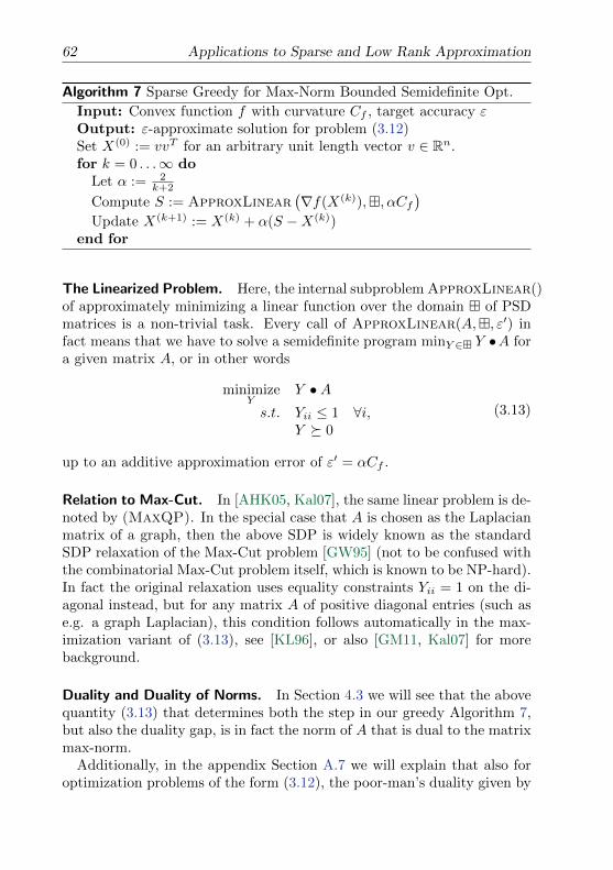
62 Applications to Sparse and Low Rank Approximation
Algorithm 7 Sparse Greedy for Max-Norm Bounded Semidefinite Opt.
Input: Convex function f with curvature Cf , target accuracy εOutput: ε-approximate solution for problem (3.12)Set X(0) := vvT for an arbitrary unit length vector v ∈ Rn.for k = 0 . . .∞ do
Let α := 2k+2
Compute S := ApproxLinear(∇f(X(k)),, αCf
)Update X(k+1) := X(k) + α(S −X(k))
end for
The Linearized Problem. Here, the internal subproblem ApproxLinear()of approximately minimizing a linear function over the domain of PSDmatrices is a non-trivial task. Every call of ApproxLinear(A,, ε′) infact means that we have to solve a semidefinite program minY ∈ Y •A fora given matrix A, or in other words
minimizeY
Y •As.t. Yii ≤ 1 ∀i,
Y 0
(3.13)
up to an additive approximation error of ε′ = αCf .
Relation to Max-Cut. In [AHK05, Kal07], the same linear problem is de-noted by (MaxQP). In the special case that A is chosen as the Laplacianmatrix of a graph, then the above SDP is widely known as the standardSDP relaxation of the Max-Cut problem [GW95] (not to be confused withthe combinatorial Max-Cut problem itself, which is known to be NP-hard).In fact the original relaxation uses equality constraints Yii = 1 on the di-agonal instead, but for any matrix A of positive diagonal entries (such ase.g. a graph Laplacian), this condition follows automatically in the max-imization variant of (3.13), see [KL96], or also [GM11, Kal07] for morebackground.
Duality and Duality of Norms. In Section 4.3 we will see that the abovequantity (3.13) that determines both the step in our greedy Algorithm 7,but also the duality gap, is in fact the norm of A that is dual to the matrixmax-norm.
Additionally, in the appendix Section A.7 we will explain that also foroptimization problems of the form (3.12), the poor-man’s duality given by
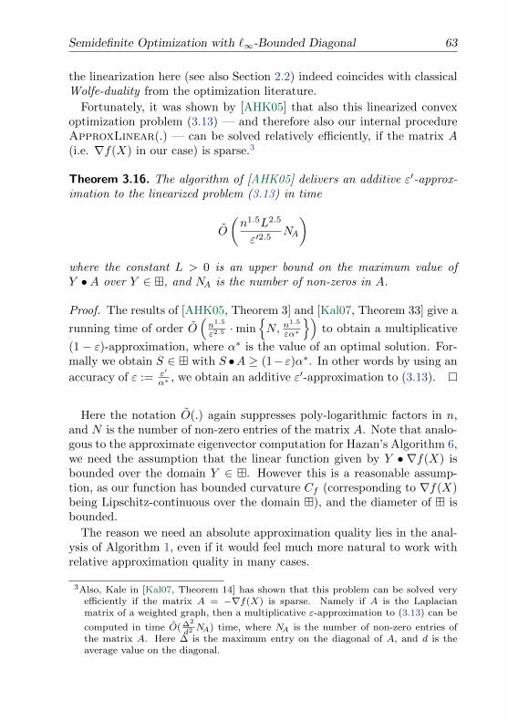
Semidefinite Optimization with `∞-Bounded Diagonal 63
the linearization here (see also Section 2.2) indeed coincides with classicalWolfe-duality from the optimization literature.
Fortunately, it was shown by [AHK05] that also this linearized convexoptimization problem (3.13) — and therefore also our internal procedureApproxLinear(.) — can be solved relatively efficiently, if the matrix A(i.e. ∇f(X) in our case) is sparse.3
Theorem 3.16. The algorithm of [AHK05] delivers an additive ε′-approx-imation to the linearized problem (3.13) in time
O
(n1.5L2.5
ε′2.5NA
)where the constant L > 0 is an upper bound on the maximum value ofY •A over Y ∈ , and NA is the number of non-zeros in A.
Proof. The results of [AHK05, Theorem 3] and [Kal07, Theorem 33] give a
running time of order O(n1.5
ε2.5 ·minN, n
1.5
εα∗
)to obtain a multiplicative
(1− ε)-approximation, where α∗ is the value of an optimal solution. For-mally we obtain S ∈ with S •A ≥ (1− ε)α∗. In other words by using an
accuracy of ε := ε′
α∗ , we obtain an additive ε′-approximation to (3.13).
Here the notation O(.) again suppresses poly-logarithmic factors in n,and N is the number of non-zero entries of the matrix A. Note that analo-gous to the approximate eigenvector computation for Hazan’s Algorithm 6,we need the assumption that the linear function given by Y • ∇f(X) isbounded over the domain Y ∈ . However this is a reasonable assump-tion, as our function has bounded curvature Cf (corresponding to ∇f(X)being Lipschitz-continuous over the domain ), and the diameter of isbounded.
The reason we need an absolute approximation quality lies in the anal-ysis of Algorithm 1, even if it would feel much more natural to work withrelative approximation quality in many cases.
3Also, Kale in [Kal07, Theorem 14] has shown that this problem can be solved veryefficiently if the matrix A = −∇f(X) is sparse. Namely if A is the Laplacianmatrix of a weighted graph, then a multiplicative ε-approximation to (3.13) can be
computed in time O( ∆2
d2NA) time, where NA is the number of non-zero entries of
the matrix A. Here ∆ is the maximum entry on the diagonal of A, and d is theaverage value on the diagonal.
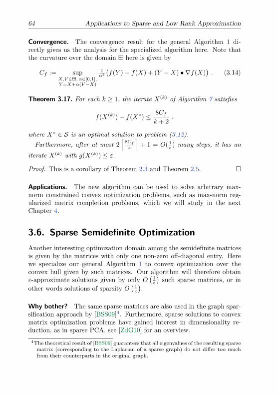
64 Applications to Sparse and Low Rank Approximation
Convergence. The convergence result for the general Algorithm 1 di-rectly gives us the analysis for the specialized algorithm here. Note thatthe curvature over the domain here is given by
Cf := supX,V ∈, α∈[0,1],Y=X+α(V−X)
1α2
(f(Y )− f(X) + (Y −X) • ∇f(X)
). (3.14)
Theorem 3.17. For each k ≥ 1, the iterate X(k) of Algorithm 7 satisfies
f(X(k))− f(X∗) ≤ 8Cfk + 2
.
where X∗ ∈ S is an optimal solution to problem (3.12).
Furthermore, after at most 2⌈
8Cfε
⌉+ 1 = O( 1
ε ) many steps, it has an
iterate X(k) with g(X(k)) ≤ ε.
Proof. This is a corollary of Theorem 2.3 and Theorem 2.5.
Applications. The new algorithm can be used to solve arbitrary max-norm constrained convex optimization problems, such as max-norm reg-ularized matrix completion problems, which we will study in the nextChapter 4.
3.6. Sparse Semidefinite Optimization
Another interesting optimization domain among the semidefinite matricesis given by the matrices with only one non-zero off-diagonal entry. Herewe specialize our general Algorithm 1 to convex optimization over theconvex hull given by such matrices. Our algorithm will therefore obtainε-approximate solutions given by only O
(1ε
)such sparse matrices, or in
other words solutions of sparsity O(
1ε
).
Why bother? The same sparse matrices are also used in the graph spar-sification approach by [BSS09]4. Furthermore, sparse solutions to convexmatrix optimization problems have gained interest in dimensionality re-duction, as in sparse PCA, see [ZdG10] for an overview.
4The theoretical result of [BSS09] guarantees that all eigenvalues of the resulting sparsematrix (corresponding to the Laplacian of a sparse graph) do not differ too muchfrom their counterparts in the original graph.
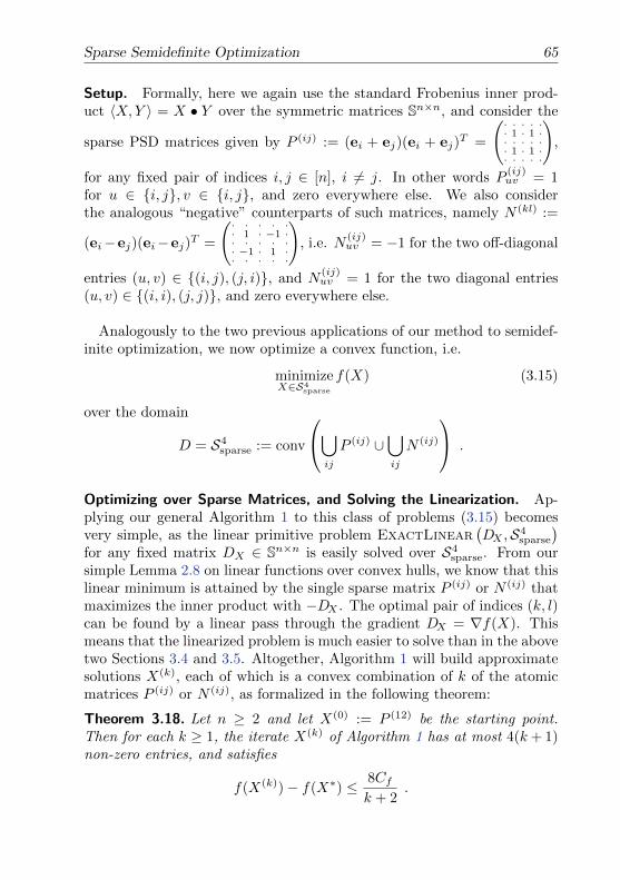
Sparse Semidefinite Optimization 65
Setup. Formally, here we again use the standard Frobenius inner prod-uct 〈X,Y 〉 = X • Y over the symmetric matrices Sn×n, and consider the
sparse PSD matrices given by P (ij) := (ei + ej)(ei + ej)T =
(· · · · ·· 1 · 1 ·· · · · ·· 1 · 1 ·· · · · ·
),
for any fixed pair of indices i, j ∈ [n], i 6= j. In other words P(ij)uv = 1
for u ∈ i, j, v ∈ i, j, and zero everywhere else. We also considerthe analogous “negative” counterparts of such matrices, namely N (kl) :=
(ei−ej)(ei−ej)T =
(· · · · ·· 1 · −1 ·· · · · ·· −1 · 1 ·· · · · ·
), i.e. N
(ij)uv = −1 for the two off-diagonal
entries (u, v) ∈ (i, j), (j, i), and N(ij)uv = 1 for the two diagonal entries
(u, v) ∈ (i, i), (j, j), and zero everywhere else.
Analogously to the two previous applications of our method to semidef-inite optimization, we now optimize a convex function, i.e.
minimizeX∈S4
sparse
f(X) (3.15)
over the domain
D = S4sparse := conv
⋃ij
P (ij) ∪⋃ij
N (ij)
.
Optimizing over Sparse Matrices, and Solving the Linearization. Ap-plying our general Algorithm 1 to this class of problems (3.15) becomesvery simple, as the linear primitive problem ExactLinear
(DX ,S4
sparse
)for any fixed matrix DX ∈ Sn×n is easily solved over S4
sparse. From oursimple Lemma 2.8 on linear functions over convex hulls, we know that thislinear minimum is attained by the single sparse matrix P (ij) or N (ij) thatmaximizes the inner product with −DX . The optimal pair of indices (k, l)can be found by a linear pass through the gradient DX = ∇f(X). Thismeans that the linearized problem is much easier to solve than in the abovetwo Sections 3.4 and 3.5. Altogether, Algorithm 1 will build approximatesolutions X(k), each of which is a convex combination of k of the atomicmatrices P (ij) or N (ij), as formalized in the following theorem:
Theorem 3.18. Let n ≥ 2 and let X(0) := P (12) be the starting point.Then for each k ≥ 1, the iterate X(k) of Algorithm 1 has at most 4(k+ 1)non-zero entries, and satisfies
f(X(k))− f(X∗) ≤ 8Cfk + 2
.
66 Applications to Sparse and Low Rank Approximation
where X∗ ∈ S4sparse is an optimal solution to problem (3.15).
Furthermore, for any ε > 0, after at most 2⌈
8Cfε
⌉+ 1 = O
(1ε
)many
steps, it has an iterate X(k) of only O(
1ε
)many non-zero entries, satisfying
g(X(k)) ≤ ε.
Proof. This is a corollary of Theorem 2.3 and Theorem 2.5. The spar-sity claim follows from our observation that the step directions given byExactLinear
(∇f(X),S4
sparse
)are always given by one of the sparse ma-
trices P (ij) or N (ij).
Optimizing over Non-Negative Matrix Factorizations. We also considerthe slight variant of (3.15), namely optimizing only over one of the twotypes of matrices as the domain D, i.e. only combinations of positiveP (ij) or only of negative N (ij). This means that the domain is given by
D = S4+sparse := conv
(⋃ij P
(ij))
or D = S4−sparse := conv
(⋃ij N
(ij))
. The
above analysis for Algorithm 1 holds in exactly the same way. Now forS4+
sparse, each step direction s = s(k) used by the algorithm is given by
s = P (ij) = (ei + ej)(ei + ej)T for some i, j, and so we have that each
of the approximations X(k) is a sum of k many positive rank-1 factorsof this form. In other words in each step k, X(k) = LRT is a productof two (entry-wise) non-negative matrices of at most k columns each, i.e.L ∈ Rn×k and Rn×k. Consequently, our algorithm provides solutions thatare non-negative matrix factorizations, which is a successful technique inmatrix completion problems from recommender systems, see e.g. [Wu07].
Relation to Bounded Trace and Diagonally Dominant Matrices. Ob-serve the matrices in S4
sparse form a subset of the bounded trace PSDmatrices S that we studied in the previous Section 3.4, since every matrixP (ij) or N (ij) is PSD and has trace equal two. Furthermore, we observethat all matrices X ∈ S4
sparse are diagonally dominant, meaning that
|Xii| ≥∑j 6=i|Xij | ∀i ∈ [n]
In the case that we restrict to using only one of the two types of matri-ces S4+
sparse or S4−sparse as the domain, then we have that equality |Xii| =∑
j 6=i |Xij | always holds, since this equality is preserved under taking con-
vex combinations, and holds for the atomic matrices P (ij) and N (ij).
Submodular Optimization 67
The Curvature. The above reasoning also implies that the curvature Cffor problems of the form (3.15) is upper bounded by the curvature in thespectahedron-case as given in (3.7), since S4+
sparse ⊆ S4sparse ⊆ 2 · S.
Applications and Future Research. Computationally, the approach herelooks very attractive, as the cost of a “sparse” step here is much cheaperthan an approximate eigenvector computation which is needed in thebounded trace case as explained in Section 3.4.
Also, it will be interesting to see how a regularization by constraining toa scaled domain S4
sparse or S4+sparse will perform in practical machine learning
applications as for example dimensionality reduction, compared to nuclearnorm regularization that we will discuss in the following Chapter 4.
It also remains to investigate further on whether we can approximategeneral bounded trace semidefinite problems of the form (3.5) by usingonly sparse matrices.
3.7. Submodular Optimization
For a finite ground set S, a real valued function defined on all subsets ofS, is called submodular, if
g(X ∩ Y ) + g(X ∪ Y ) ≤ g(X) + g(Y ) ∀X,Y ⊆ S
For any given submodular function g with g(∅) = 0, the paper [Lov83,Section 3] introduces a corresponding convex set in R|S|, called the sub-modular polyhedron (or also Lovasz polyhedron),
Pg :=
x ∈ R|S|
∣∣∣∣∣ ∑i∈T
xi ≤ g(T ) ∀T ⊆ S
.
We would now like to study convex optimization problems over such do-mains, which become compact convex sets if we intersect with the positive
orthant, i.e. D := Pg ∩ R|S|≥0.Nicely for our optimization framework, [Lov83, Section 3] already showed
that there is a simple greedy algorithm which optimizes any linear functionover the domain Pg, i.e. it solves max
x∈PgcTx, or in other words it exactly
solves our internal problem ExactLinear (c,Pg).Lovasz [Lov83] already demonstrated how to use this kind of linear opti-
mization over Pg to solve submodular minimization problems. It remains

68 Applications to Sparse and Low Rank Approximation
to investigate if there are interesting applications for the wider class ofmore general convex (non-linear) functions f over such domains, as ad-dressed by our Algorithm 1.
4Optimization with the
Nuclear and Max-Norm
Matrix optimization problems with a nuclear norm or max-norm regular-ization, such as e.g. low norm matrix factorizations, have seen many appli-cations recently, ranging from low-rank recovery, dimensionality reduction,to recommender systems. We propose two new first-order approximationmethods building upon two of the simple semidefinite optimizers from theprevious Chapter, that is the approximate SDP solver of [Haz08] fromSection 3.4 on one hand, and our bounded diagonal optimizer from Sec-tion 3.5 on the other hand. The algorithms come with strong convergenceguarantees.
In contrast to existing methods, our nuclear norm optimizer does notneed any Cholesky or singular value decompositions internally, and pro-vides guaranteed approximations that are simultaneously of low rank. Themethod is free of tuning parameters, and easy to parallelize.
4.1. Introduction
In this chapter we consider convex optimization problems over matrices,which come with a regularization on either the nuclear norm or the max-norm of the optimization variable.
69
70 Optimization with the Nuclear and Max-Norm
Convex optimization with the nuclear norm has become a very success-ful technique in various machine learning, computer vision and compressedsensing areas such as low-rank recovery [FHB01, CR09, CT10], dimension-ality reduction (such as robust principal component analysis [CLMW11]),and also recommender systems and matrix completion. Here matrix fac-torizations [SRJ04, KBV09] — regularized by the nuclear or max-norm —have gained a lot of attention with the recently ended Netflix Prize com-petition. Many more applications of similar optimization problems can befound among dimensionality reduction, matrix classification, multi-tasklearning, spectral clustering and others. The success of these methods isfueled by the property of the nuclear norm being a natural convex relax-ation of the rank, allowing the use of scalable convex optimization tech-niques.
Based on the semidefinite optimization methods that we have presentedin the above Sections 3.4 and 3.5, we propose two new, yet simple, first-order algorithms for nuclear norm as well as max-norm regularized convexoptimization.
For the nuclear norm case, our proposed method builds upon the first-order scheme for semidefinite optimization by [Haz08], which we have in-vestigated in Section 3.4.1. This approach allows us to significantly reducethe computational complexity per iteration, and therefore scale to muchlarger datasets: While existing methods need an entire and exact singularvalue decomposition (SVD) in each step, our method only uses a singleapproximate eigenvector computation per iteration, which can be done bye.g. the power method. A conference version of our work for nuclear normregularized problems has appeared in [JS10].
In the same spirit, we will also give a new algorithm with a convergenceguarantee for optimizing with a max-norm regularization. For matrix com-pletion problems, experiments show that the max-norm can result in animproved generalization performance compared to the nuclear norm insome cases [SRJ04, LRS+10].
Nuclear Norm Regularized Convex Optimization. We consider the fol-lowing convex optimization problems over matrices:
minZ∈Rm×n
f(Z) + µ ‖Z‖∗ (4.1)
and the corresponding constrained variant
minZ∈Rm×n, ‖Z‖∗≤ t2
f(Z) (4.2)
Introduction 71
where f(Z) is any differentiable convex function (usually called the lossfunction), ‖.‖∗ is the nuclear norm of a matrix, also known as the tracenorm (sum of the singular values, or `1-norm of the spectrum). Hereµ > 0 and t > 0 respectively are given parameters, usually called theregularization parameter.
The nuclear norm is know as the natural generalization of the (sparsityinducing) `1-norm for vectors, to the case of semidefinite matrices. When
choosing f(X) := ‖A(X)− b‖22 for some linear map A : Rn×m → Rp,the above formulation (4.1) is the matrix generalization of the problem
minx∈Rn ‖Ax− b‖22 + µ ‖x‖1, for a fixed matrix A, which is the important`1-regularized least squares problem, also known as the basis pursuit de-noising problem in the compressed sensing literature, see also Section 3.2.1.The analoguous vector variant of (4.2) is the Lasso problem [Tib96] which
is minx∈Rn‖Ax− b‖22
∣∣∣ ‖x‖1 ≤ t.
Max-Norm Regularized Convex Optimization. Intuitively, one can thinkof the matrix max-norm as the generalization of the vector `∞-norm toPSD matrices. Here we consider optimization problems with a max-normregularization, which are given by
minZ∈Rm×n
f(Z) + µ ‖Z‖max (4.3)
and the corresponding constrained variant being
minZ∈Rm×n, ‖Z‖max≤t
f(Z) . (4.4)
Our Contribution. Applying our general optimization method from theprevious Chapters 2 and 3, we present a much simpler algorithm to solveproblems of the form (4.2), which does not need any internal SVD com-putations. The same approach will also solve the max-norm regularizedproblems (4.4). We achieve this by transforming the problems to the con-vex optimization setting over positive semidefinite matrices which we havestudied in the above Sections 3.4.1 and 3.5.
Our new approach has several advantages for nuclear norm optimiza-tion when compared to the existing algorithms such as “proximal gradient”methods (APG) and “singular value thresholding” (SVT), see e.g. [GLW+09,CCS10, TY10, JY09], and also in comparison to the alternating-gradient-descent-type methods (as e.g. [RS05, Lin07]).
72 Optimization with the Nuclear and Max-Norm
i) By employing the approximate SDP solver by [Haz08], see Algo-rithm 6, we obtain a guaranteed ε-approximate solution Z afterO(
1ε
)iterations. Crucially, the resulting solution Z is simultane-
ously of low rank, namely rank O(
1ε
). Also the algorithm main-
tains a compact representation of Z in terms of a low-rank matrixfactorization Z = LRT (with the desired bounded nuclear norm),and can therefore even be applied if the full matrix Z would be fartoo large to even be stored.
ii) Compared to the alternating-gradient-descent-type methods frommachine learning, we overcome the problem of working with non-convex formulations of the form f(LRT ), which is NP-hard, andinstead solve the original convex problem in f(Z).
iii) The total running time of our algorithm for nuclear norm problemsgrows linear in the problem size, allows to take full advantage ofsparse problems such as e.g. for matrix completion. More precisely,
the algorithm runs in time O(Nfε1.5
), where Nf is the number of
matrix entries on which the objective function f depends. Per it-eration, our method consists of only a single approximate (largest)eigenvector computation, allowing it to scale to any problem sizewhere the power method (or Lanczos’ algorithm) can still be ap-plied. This also makes the method easy to implement and to par-allelize. Existing APG/SVT methods by contrast need an entireSVD in each step, which is significantly more expensive.
iv) On the theory side, our simple convergence guarantee of O(
1ε
)steps holds even if the used eigenvectors are only approximate. Incomparison, those existing methods that come with a convergenceguarantee do require an exact SVD in each iteration, which mightnot always be a realistic assumption in practice.
We demonstrate that our new algorithm on standard datasets improvesover the state of the art methods, and scales to large problems such asmatrix factorizations on the Netflix dataset.
Hazan’s Algorithm 6 can be interpreted as the generalization of thecoreset approach to problems on symmetric matrices, which we have ex-plained in the previous Section 3.4.1. Compared to the O(1/
√ε) conver-
gence methods in the spirit of [Nes83, Nes07a], our number of steps islarger, which is however more than compensated by the improved stepcomplexity, being lower by a factor of roughly (n+m).
Our new method for the nuclear norm case can also be interpreted asa modified, theoretically justified variant of Simon Funk’s popular SVD
Introduction 73
heuristic [Web06] for regularized matrix factorization. To our knowledgethis is the first guaranteed convergence result for this class of alternating-gradient-descent-type algorithms.
Related Work. For nuclear norm optimization, there are two lines of ex-isting methods. On the one hand, in the optimization community, [TY10,LST09], [GLW+09] and [JY09] independently proposed algorithms thatobtain an ε-accurate solution to (4.1) in O(1/
√ε) steps, by improving the
algorithm of [CCS10]. These methods are known under the names “acceler-ated proximal gradient” (APG) and “singular value thresholding” (SVT).More recently also [MHT10] and [MGC09] proposed algorithms along thesame idea. Each step of all those algorithms requires the computation ofthe singular value decomposition (SVD) of a matrix of the same size as thesolution matrix, which is expensive even with the currently available fastmethods such as PROPACK. [TY10] and [JY09] and also [GLW+09] showthat the primal error of their algorithm is smaller than ε after O(1/
√ε)
steps, using an analysis inspired by [Nes83] and [BT09]. For an overview ofrelated algorithms, we also refer the reader to [CLMW11]. As mentionedabove, the method presented here has a significantly lower computationalcost per iteration (one approximate eigenvector compared to a full exactSVD), and is also faster in practice on large matrix completion problems.
On the other hand, in the machine learning community, research origi-nated from matrix completion and factorization [SRJ04], later motivatedby the Netflix prize challenge, getting significant momentum from the fa-mous blog post by [Web06]. Only very recently an understanding hasformed that many of these methods can indeed by seen as optimizing withregularization term closely related to the nuclear norm, see Section 4.5.4and [SS10]. The majority of the currently existing machine learning meth-ods such as for example [RS05, Lin07] and later also [Pat07, ZWSP08,KBV09, TPNT09, IR10, GNHS11] are of the type of “alternating” gradi-ent descent applied to f(LRT ), where at each step one of the factors L andR is kept fixed, and the other factor is updated by a gradient or stochasticgradient step. Therefore, despite working well in many practical applica-tions, all these mentioned methods can get stuck in local minima — andso are theoretically not well justified, see also the discussion in [DeC06]and our Section 4.4.
The same issue also comes up for max-norm optimization, where forexample [LRS+10] optimize over the non-convex factorization (4.8) forbounded max-norm. To our knowledge, no algorithm with a convergenceguarantee was known so far.
74 Optimization with the Nuclear and Max-Norm
Furthermore, optimizing with a rank constraint was recently shown tobe NP-hard [GG10]. In practical applications, nearly all approaches forlarge scale problems are working over a factorization Z = LRT of boundedrank, therefore ruling out their ability to obtain a solution in polynomialtime in the worst-case, unless P = NP.
Our new method for both nuclear and max-norm avoids all the abovedescribed problems by solving an equivalent convex optimization problem,and provably runs in near linear time in the nuclear norm case.
4.2. The Nuclear Norm for Matrices
The nuclear norm ‖Z‖∗ of a rectangular matrix Z ∈ Rm×n, also knownas the trace norm or Ky Fan norm, is given by the sum of the singularvalues of Z, which is equal to the `1-norm of the singular values of Z(because singular values are always non-negative). Therefore, the nuclearnorm is often called the Schatten `1-norm. In this sense, it is a naturalgeneralization of the `1-norm for vectors which we have studied earlier.
The nuclear norm has a nice equivalent characterization in terms ofmatrix factorizations of Z, i.e.
‖Z‖∗ := minLRT=Z
1
2
(‖L‖2Fro + ‖R‖2Fro
), (4.5)
where the number of columns of the factors L ∈ Rm×k and Rn×k is notconstrained [FHB01, SRJ04]. In other words, the nuclear norm constrainsthe average Euclidean row or column norms of any factorization of theoriginal matrix Z.
Furthermore, the nuclear norm is dual to the standard spectral matrixnorm (i.e. the matrix operator norm), meaning that
‖Z‖∗ = maxB,‖B‖spec≤1
B • Z ,
see also [RFP10]. Recall that ‖B‖spec is defined as the first singular valueσ1(B) of the matrix B.
Similarly to the property of the vector ‖.‖1-norm being the best convexapproximation to the sparsity of a vector, as we discussed in Section 3.2the nuclear norm is the best convex approximation of the matrix rank.More precisely, ‖.‖∗ is the convex envelope of the rank [FHB01], meaningthat it is the largest convex function that is upper bounded by the rank on
the convex domain of matricesZ∣∣∣ ‖Z‖spec ≤ 1
. This motivates why
The Nuclear Norm for Matrices 75
the nuclear norm is widely used as a proxy function (or convex relaxation)for rank minimization, which otherwise is a hard combinatorial problem.
Its relation to semidefinite optimization — which explains why the nu-clear norm is often called the trace norm — is that
‖Z‖∗ = minimizeV,W
t
s.t.
(V ZZT W
) 0 and
Tr(V ) + Tr(W ) ≤ 2t .
(4.6)
Here the two optimization variables range over the symmetric matri-ces V ∈ Sm×m and W ∈ Sn×n. This semidefinite characterization willin fact be the central tool for our algorithmic approach for nuclear normregularized problems in the following. The equivalence of the above charac-terization to the earlier “factorization” formulation (4.5) is a consequenceof the following simple Lemma 4.1. The Lemma gives a correspondencebetween the (rectangular) matrices Z ∈ Rm×n of bounded nuclear normon one hand, and the (symmetric) PSD matrices X ∈ S(m+n)×(m+n) ofbounded trace on the other hand.
Lemma 4.1 ([FHB01, Lemma 1]). For any non-zero matrix Z ∈ Rm×n andt ∈ R, it holds that
‖Z‖∗ ≤t
2if and only if
∃ symmetric matrices V ∈ Sm×m,W ∈ Sn×n
s.t.
(V ZZT W
) 0 and Tr(V ) + Tr(W ) ≤ t .
Proof. ⇒ Using the characterization (4.5) of the nuclear norm ‖Z‖∗ =
minLRT=Z12 (‖L‖2Fro+‖R‖2Fro) we get that ∃ L,R, LRT = Z s.t. ‖L‖2Fro+
‖R‖2Fro = Tr(LLT ) + Tr(RRT ) ≤ t, or in other words we have found a
matrix(LLT ZZT RRT
)= (LR)(LR)T 0 of trace ≤ t.
⇐ As the matrix(V ZZT W
)is symmetric and PSD, it can be (Cholesky)
factorized to (L;R)(L;R)T s.t. LRT = Z and t ≥ Tr(LLT ) + Tr(RRT ) =
‖L‖2Fro + ‖R‖2Fro, therefore ‖Z‖∗ ≤ t2 .
Interestingly, for characterizing bounded nuclear norm matrices, it doesnot make any difference whether we enforce an equality or inequality con-straint on the trace. This fact will turn out to be useful in order to applyour Algorithm 6 later on.
76 Optimization with the Nuclear and Max-Norm
Corollary 4.2. For any non-zero matrix Z ∈ Rm×n and t ∈ R, it holds that
‖Z‖∗ ≤t
2
if and only if
∃ symmetric matrices V ∈ Sm×m,W ∈ Sn×n
s.t.
(V ZZT W
) 0 and Tr(V ) + Tr(W ) = t .
Proof. ⇒ From Lemma 4.1 we obtain a matrix(V ZZT W
)=: X 0 of
trace say s ≤ t. If s < t, we add (t− s) to the top-left entry of V , i.e. weadd to X the PSD rank-1 matrix (t − s)e1e
T1 (which again gives a PSD
matrix). ⇐ follows directly from Lemma 4.1.
4.2.1. Weighted Nuclear Norm
A promising weighted nuclear norm regularization for matrix completionwas recently proposed by [SS10]. For fixed weight vectors p ∈ Rm, q ∈ Rn,the weighted nuclear norm ‖Z‖nuc(p,q) of Z ∈ Rm×n is defined as
‖Z‖nuc(p,q) := ‖PZQ‖∗ ,
where P = diag(√p) ∈ Rm×m denotes the diagonal matrix whose i-th
diagonal entry is√pi, and analogously for Q = diag(
√q) ∈ Rn×n. Here
p ∈ Rm is the vector whose entries are the probabilities p(i) > 0 that thei-th row is observed in the sampling Ω. Analogously, q ∈ Rn contains theprobability q(j) > 0 for each column j. The opposite weighting (using 1
p(i)
and 1q(j) instead of p(i),q(j)) has also been suggested by [WKS08].
Any optimization problem with a weighted nuclear norm regularization
minZ∈Rm×n, ‖Z‖nuc(p,q)≤ t/2
f(Z) (4.7)
and arbitrary loss function f can therefore be formulated equivalently overthe domain ‖PZQ‖∗ ≤ t/2, such that it reads as (if we substitute Z :=PZQ),
minZ∈Rm×n,‖Z‖∗≤ t/2
f(P−1ZQ−1).
Hence, we have reduced the task to our standard convex problem (4.2) for
f that here is defined as
f(X) := f(P−1ZQ−1),
The Max-Norm for Matrices 77
where X =:(V ZZTW
). This equivalence implies that any algorithm solv-
ing (4.2) also serves as an algorithm for weighted nuclear norm regulariza-tion. In particular, Hazan’s Algorithm 6 does imply a guaranteed approx-imation quality of ε for problem (4.7) after O
(1ε
)many rank-1 updates,
as we discussed in Section 3.4. So far, to the best of our knowledge, noapproximation guarantees were known for the weighted nuclear norm.
We will discuss solution path algorithms (maintaining approximationguarantees when the regularization parameter t changes) also for the weightednuclear norm case in Chapter 7.
4.3. The Max-Norm for Matrices
We think of the matrix max-norm as a generalization of the vector `∞-norm to the case of positive semidefinite matrices, which we have studiedbefore.
In some matrix completion applications, the max-norm has been ob-served to provide solutions of better generalization performance than thenuclear norm [SRJ04]. Both matrix norms can be seen as a convex surro-gate of the rank [SS05].
The max-norm ‖Z‖max of a rectangular matrix Z ∈ Rm×n has a nicecharacterization in terms of matrix factorizations of Z, i.e.
‖Z‖max := minLRT=Z
max‖L‖22,∞ , ‖R‖22,∞ , (4.8)
where the number of columns of the factors L ∈ Rm×k and Rn×k is notconstrained [LRS+10]. Here ‖L‖2,∞ is the maximum `2-norm of any row
Li: of L, that is ‖L‖2,∞ := maxi ‖Li:‖2 = maxi√∑
k L2ik. Compared to
the nuclear norm, we therefore observe that the max-norm constrains themaximal Euclidean row-norms of any factorization of the original matrixZ, see also [SS05]. 1
An alternative formulation of the max-norm was given by [LMSS07]and [SS05], stating that
‖Z‖max = minLRT=Z
(maxi||Li:||2)(max
i||Ri:||2) .
1Note that the max-norm does not coincide with the matrix norm induced by the
vector ‖.‖∞-norm, that is ‖Z‖∞ := supx 6=0‖Zx‖∞‖x‖∞
. The latter matrix norm by
contrast is known to be the maximum of the row sums of Z (i.e. the `1-norms ofthe rows).
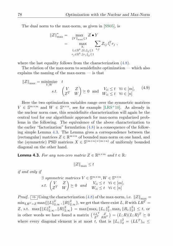
78 Optimization with the Nuclear and Max-Norm
The dual norm to the max-norm, as given in [SS05], is
‖Z‖∗max = max‖Y ‖max≤1
Z • Y
= maxk,
li∈Rk,‖li‖2≤1
rj∈Rk,‖rj‖2≤1
∑i,j
Zij lTi rj ,
where the last equality follows from the characterization (4.8).The relation of the max-norm to semidefinite optimization — which also
explains the naming of the max-norm — is that
‖Z‖max = minimizeV,W
t
s.t.
(V ZZT W
) 0 and
Vii ≤ t ∀i ∈ [m],Wii ≤ t ∀i ∈ [n]
(4.9)
Here the two optimization variables range over the symmetric matricesV ∈ Sm×m and W ∈ Sn×n, see for example [LRS+10]. As already inthe nuclear norm case, this semidefinite characterization will again be thecentral tool for our algorithmic approach for max-norm regularized prob-lems in the following. The equivalence of the above characterization tothe earlier “factorization” formulation (4.8) is a consequence of the follow-ing simple Lemma 4.3. The Lemma gives a correspondence between the(rectangular) matrices Z ∈ Rm×n of bounded max-norm on one hand, andthe (symmetric) PSD matrices X ∈ S(m+n)×(m+n) of uniformly boundeddiagonal on the other hand.
Lemma 4.3. For any non-zero matrix Z ∈ Rn×m and t ∈ R:
‖Z‖max ≤ tif and only if
∃ symmetric matrices V ∈ Sm×m,W ∈ Sn×n
s.t.
(V ZZT W
) 0 and
Vii ≤ t ∀i ∈ [m],Wii ≤ t ∀i ∈ [n]
Proof. ⇒ Using the characterization (4.8) of the max-norm, i.e. ‖Z‖max =
minLRT=Z max‖L‖22,∞ , ‖R‖22,∞, we get that there exist L,R with LRT =
Z, s.t. max‖L‖22,∞ , ‖R‖22,∞ = maxmaxi ‖Li:‖22 ,maxi ‖Ri:‖22 ≤ t, or
in other words we have found a matrix(LLT ZZT RRT
)= (L;R)(L;R)T 0
where every diagonal element is at most t, that is ‖Li:‖22 = (LLT )ii ≤
Optimizing with Bounded Nuclear Norm and Max-Norm 79
t ∀i ∈ [m], and ‖Ri:‖22 = (RRT )ii ≤ t ∀i ∈ [n].⇐ As the matrix
(V ZZT W
)is symmetric and PSD, it can be (Cholesky)
factorized to (L;R)(L;R)T s.t. LRT = Z and ‖Li:‖22 = (LLT )ii ≤ t ∀i ∈[m] and ‖Ri:‖22 = (RRT )ii ≤ t ∀i ∈ [n], which implies ‖Z‖max ≤ t.
4.4. Optimizing with Bounded Nuclear Normand Max-Norm
Most of the currently known algorithms for matrix factorizations as wellas nuclear norm or max-norm regularized optimization problems, suchas (4.1), (4.2), (4.3) or (4.4), do suffer from the following problem:
In order to optimize the convex objective function f(Z) while controllingthe norm ‖Z‖∗ or ‖Z‖max, the methods instead try to optimize f(LRT ),with respect to both factors L ∈ Rm×k and R ∈ Rn×k, with the corre-sponding regularization constraint imposed on L and R. This approach isof course very tempting, as the constraints on the factors — which orig-inate from the matrix factorization characterizations (4.5) and (4.8) —are simple and in some sense easier to enforce.
Unhealthy Side-Effects of Factorizing. However, there is a significantprice to pay: Even if the objective function f(Z) is convex in Z, the verysame function expressed as a function f(LRT ) of both the factor variablesL and R becomes a severely non-convex problem, naturally consisting of alarge number of saddle-points (consider for example just the smallest caseL,R ∈ R1×1 together with the identity function f(Z) = Z ∈ R).
The majority of the currently existing methods such as for example [RS05,Lin07] and later also [Pat07, ZWSP08, KBV09, TPNT09, IR10, GNHS11]is of this “alternating” gradient descent type, where at each step one ofthe factors L and R is kept fixed, and the other factor is updated by e.g.a gradient or stochastic gradient step. Therefore, despite working well inmany practical applications, all these mentioned methods can get stuckin local minima — and so are theoretically not well justified, see also thediscussion in [DeC06].
The same issue also comes up for max-norm optimization, where forexample [LRS+10] optimize over the non-convex factorization (4.8) forbounded max-norm.
Concerning the fixed rank of the factorization, [GG10] have shown thatfinding the optimum under a rank constraint (even if the rank is one) is
80 Optimization with the Nuclear and Max-Norm
NP-hard (here the used function f was the standard squared error on anincomplete matrix). On the positive side, [BM03] have shown that if therank k of the factors L and R exceeds the rank of the optimum solutionX∗, then — in some cases — it can be guaranteed that the local minima(or saddle points) are also global minima. However, in nearly all practi-cal applications it is computationally infeasible for the above mentionedmethods to optimize with the rank k being in the same order of magnitudeas the original matrix size m and n (as e.g. in the Netflix problem, suchfactors L,R could possibly not even be stored on a single machine2).
Relief: Optimizing Over an Equivalent Convex Problem. Here we sim-ply overcome this problem by using the transformation to semidefinite ma-trices, which we have outlined in the above Corollary 4.2 and Lemma 4.3.These bijections of bounded nuclear and max-norm matrices to the PSDmatrices over the corresponding natural convex domains do allow us todirectly optimize a convex problem, avoiding the factorization problemsexplained above. We describe this simple trick formally in the next twoSubsections 4.4.1 and 4.4.2.
But what if you really need a Matrix Factorization? In some applica-tions (such as for example embeddings or certain collaborative filteringproblems) of the above mentioned regularized optimization problems overf(Z), one would still want to obtain the solution (or approximation) Zin a factorized representation, that is Z = LRT . We note that this isalso straight-forward to achieve when using our transformation: An ex-plicit factorization of any feasible solution to the transformed problem (3.5)or (3.12) — if needed — can always be directly obtained since X 0.
Alternatively, algorithms for solving the transformed problem (3.5) candirectly maintain the approximate solution X in a factorized representa-tion (as a sum of rank-1 matrices), as achieved for example by Algorithms 6and 7.
4.4.1. Optimization with a Nuclear Norm Regularization
Having Lemma 4.1 at hand, we immediately get to the crucial observationof this section, allowing us to apply Algorithm 6:
2Algorithm 6 in contrast does never need to store a full estimate matrix X, butinstead just keeps the rank-1 factors v obtained in each step, maintaining a factorizedrepresentation of X.
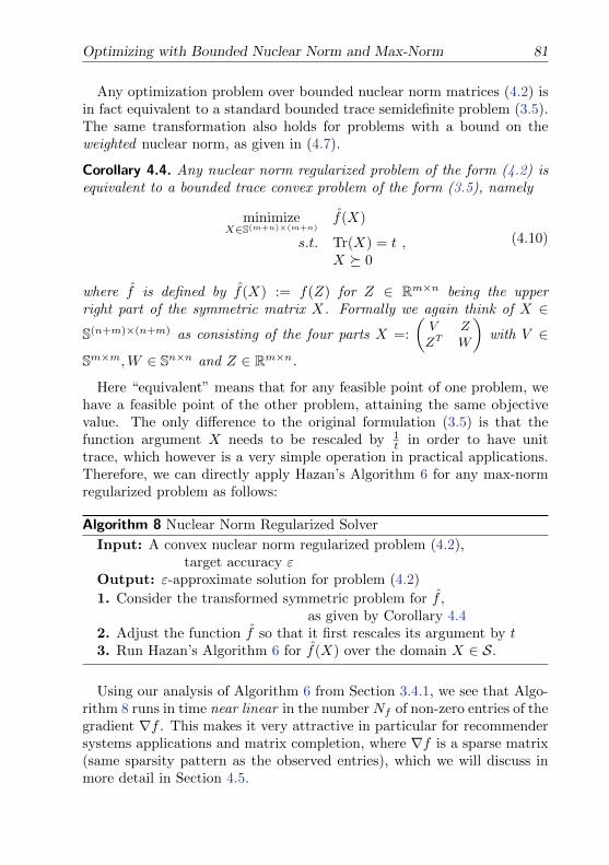
Optimizing with Bounded Nuclear Norm and Max-Norm 81
Any optimization problem over bounded nuclear norm matrices (4.2) isin fact equivalent to a standard bounded trace semidefinite problem (3.5).The same transformation also holds for problems with a bound on theweighted nuclear norm, as given in (4.7).
Corollary 4.4. Any nuclear norm regularized problem of the form (4.2) isequivalent to a bounded trace convex problem of the form (3.5), namely
minimizeX∈S(m+n)×(m+n)
f(X)
s.t. Tr(X) = t ,X 0
(4.10)
where f is defined by f(X) := f(Z) for Z ∈ Rm×n being the upperright part of the symmetric matrix X. Formally we again think of X ∈S(n+m)×(n+m) as consisting of the four parts X =:
(V ZZT W
)with V ∈
Sm×m,W ∈ Sn×n and Z ∈ Rm×n.
Here “equivalent” means that for any feasible point of one problem, wehave a feasible point of the other problem, attaining the same objectivevalue. The only difference to the original formulation (3.5) is that thefunction argument X needs to be rescaled by 1
t in order to have unittrace, which however is a very simple operation in practical applications.Therefore, we can directly apply Hazan’s Algorithm 6 for any max-normregularized problem as follows:
Algorithm 8 Nuclear Norm Regularized Solver
Input: A convex nuclear norm regularized problem (4.2),target accuracy ε
Output: ε-approximate solution for problem (4.2)
1. Consider the transformed symmetric problem for f ,as given by Corollary 4.4
2. Adjust the function f so that it first rescales its argument by t3. Run Hazan’s Algorithm 6 for f(X) over the domain X ∈ S.
Using our analysis of Algorithm 6 from Section 3.4.1, we see that Algo-rithm 8 runs in time near linear in the number Nf of non-zero entries of thegradient ∇f . This makes it very attractive in particular for recommendersystems applications and matrix completion, where ∇f is a sparse matrix(same sparsity pattern as the observed entries), which we will discuss inmore detail in Section 4.5.
82 Optimization with the Nuclear and Max-Norm
Corollary 4.5. After at most O(
1ε
)many iterations (i.e. approximate
eigenvalue computations), Algorithm 8 obtains a solution that is ε close
to the optimum of (4.2). The algorithm requires a total of O(Nfε1.5
)arith-
metic operations (with high probability).
Proof. We use the transformation from Corollary 4.4 and then rescale allmatrix entries by 1
t . Then result then follows from Corollary 3.12 onpage 56 on the running time of Hazan’s algorithm.
The fact that each iteration of our algorithm is computationally verycheap — consisting only of the computation of an approximate eigenvector— strongly contrasts the existing “proximal gradient” and “singular valuethresholding” methods [GLW+09, JY09, MGC09, LST09, CCS10, TY10],which in each step need to compute an entire SVD. Such a single incom-plete SVD computation (first k singular vectors) amounts to the samecomputational cost as an entire run of our algorithm (for k steps). Fur-thermore, those existing methods which come with a theoretical guarantee,in their analysis assume that all SVDs used during the algorithm are exact,which is not feasible in practice. By contrast, our analysis is rigorous evenif the used eigenvectors are only ε′-approximate.
Another nice property of Hazan’s method is that the returned solutionis guaranteed to be simultaneously of low rank (k after k steps), and thatby incrementally adding the rank-1 matrices vkv
Tk , the algorithm automat-
ically maintains a matrix factorization of the approximate solution.
Also, Hazan’s algorithm, as being an instance of our general frameworkfrom Chapter 2, is designed to automatically stay within the feasible regionS, where most of the existing methods do need a projection step to get backto the feasible region (as e.g. [Lin07, LST09]), making both the theoreticalanalysis and implementation more complicated.
4.4.2. Optimization with a Max-Norm Regularization
The same approach works analogously for the max-norm, by using Lemma 4.3in order to apply Algorithm 7:
Any optimization problem over bounded max-norm matrices (4.4) is infact equivalent to a semidefinite problem (3.12) over the “box” of matriceswhere each element on the diagonal is bounded above by t. We thinkof this domain as generalizing the positive cube of vectors, to the PSDmatrices.
Optimizing with Bounded Nuclear Norm and Max-Norm 83
Corollary 4.6. Any max-norm regularized problem of the form (4.4) isequivalent to a bounded diagonal convex problem of the form (3.12), i.e.,
minimizeX∈S(m+n)×(m+n)
f(X)
s.t. Xii ≤ 1 ∀i,X 0
(4.11)
where f is defined by f(X) := f(Z) for Z ∈ Rm×n being the upper rightpart of the symmetric matrix X. Formally we again think of any X ∈S(n+m)×(n+m) as consisting of the four parts X =:
(V ZZT W
)with V ∈
Sm×m,W ∈ Sn×n and Z ∈ Rm×n.
Again the only difference to the original formulation (3.12) is that thefunction argument X needs to be rescaled by 1
t in order to have the diago-nal bounded by one, which however is a very simple operation in practicalapplications. This means we can directly apply Algorithm 7 for any max-norm regularized problem as follows:
Algorithm 9 Max-Norm Regularized Solver
Input: A convex max-norm regularized problem (4.4),target accuracy ε
Output: ε-approximate solution for problem (4.4)
1. Consider the transformed symmetric problem for f ,as given by Corollary 4.6
2. Adjust the function f so that it first rescales its argument by t3. Run Algorithm 7 for f(X) over the domain X ∈ .
Using the analysis of our new Algorithm 7 from Section 3.4.1, we obtainthe following guarantee:
Corollary 4.7. After⌈
8Cfε
⌉many iterations, Algorithm 9 obtains a solution
that is ε close to the optimum of (4.4).
Proof. We use the transformation from Corollary 4.6 and then rescale allmatrix entries by 1
t . Then the running time of the algorithm follows fromTheorem 3.17.
Maximum Margin Matrix Factorizations. In the case of matrix comple-tion, the “loss” function f is defined as measuring the error from X to some
84 Optimization with the Nuclear and Max-Norm
fixed observed matrix, but just at a small fixed set of “observed” positionsof the matrices. As we already mentioned, semidefinite optimization overX as above can always be interpreted as finding a matrix factorization, asa symmetric PSD matrix X always has a (unique) Cholesky factorization.
Now for the setting of matrix completion, it is known that the above de-scribed optimization task under bounded max-norm, can be geometricallyinterpreted as learning a maximum margin separating hyperplane for eachuser/movie. In other words the factorization problem decomposes into acollection of SVMs, one for each user or movie, if we think of the corre-sponding other factor to be fixed for a moment [SRJ04]. We will discussmatrix completion in more detail in Section 4.5.
Other Applications of Max-Norm Optimization. Apart from matrixcompletion, optimization problems employing the max-norm have otherprominent applications in spectral methods, spectral graph properties,low-rank recovery, and combinatorial problems such as Max-Cut.
4.5. Applications
Our Algorithm 8 directly applies to arbitrary nuclear norm regularizedproblems of the form (4.2). Since the nuclear norm is in a sense the mostnatural generalization of the sparsity-inducing `1-norm to the case of lowrank matrices (see also the discussion in the previous chapters) there aremany applications of this class of optimization problems.
4.5.1. Robust Principal Component Analysis
One prominent example of a nuclear norm regularized problem in the areaof dimensionality reduction is given by the technique of robust PCA asintroduced by [CLMW11], also called principal component pursuit, whichis the optimization task
minZ∈Rm×n
‖Z‖∗ + µ ‖M − Z‖1 . (4.12)
Here M ∈ Rm×n is the given data matrix, and ‖.‖1 denotes the entry-wise`1-norm. By considering the equivalent constrained variant ‖Z‖∗ ≤ t
2instead, we obtain a problem the form (4.2), suitable for our Algorithm 8.However, since the original objective function f(Z) = ‖M − Z‖1 is notdifferentiable, a smoothed version of the `1-norm has to be used instead.
Applications 85
This situation is analogous to the hinge-loss objective in maximum marginmatrix factorization [SRJ04].
Existing algorithms for robust PCA do usually require a complete (andexact) SVD in each iteration, as e.g. [TY10, AGI11], and are often harderto analyze compared to our approach. The first algorithm with a con-vergence guarantee of O
(1ε
)was given by [AGI11], requiring a SVD com-
putation per step. Our Algorithm 8 obtains the same guarantee in thesame order of steps, but only requires a single approximate eigenvectorcomputation per step, which is significantly cheaper.
Last but not least, the fact that our algorithm delivers approximatesolutions to (4.12) of rank O
(1ε
)will be interesting for practical dimen-
sionality reduction applications, as it re-introduces the important conceptof low-rank factorizations as in classical PCA. In other words our algorithmproduces an embedding into at most O
(1ε
)many new dimensions, which is
much easier to deal with in practice compared to the full rank n solutionsresulting from the existing solvers for robust PCA, see e.g. [CLMW11] andthe references therein.
We did not yet perform practical experiments for robust PCA, but choseto demonstrate the practical performance of Algorithm 6 for matrix com-pletion problems first.
4.5.2. Matrix Completion and Low Norm MatrixFactorizations
For matrix completion problems as for example in collaborative filteringand recommender systems [KBV09], our algorithm is particularly suitableas it retains the sparsity of the observations, and constructs the solutionin a factorized way. In the setting of a partially observed matrix such asin the Netflix case, the loss function f(X) only depends on the observedpositions, which are very sparse, so ∇f(X) — which is all we need for ouralgorithm — is also sparse.
We want to approximate a partially given matrix Y (let Ω be the set ofknown training entries of the matrix) by a product Z = LRT such thatsome convex loss function f(Z) is minimized. By Ωtest we denote theunknown test entries of the matrix we want to predict.
Complexity. Just recently it has been shown that the standard low-rankmatrix completion problem — that is finding the best approximation toan incomplete matrix by the standard `2-norm — is an NP-hard problem,
86 Optimization with the Nuclear and Max-Norm
if the rank of the approximation is constrained. The hardness is claimedto hold even for the rank 1 case [GG10].
In the light of this hardness result, the advantage of relaxing the rankby replacing it by the nuclear norm (or max-norm) is even more evident.
Our near linear time Algorithm 8 relies on a convex optimization formu-lation and does indeed deliver an guaranteed ε-accurate solution for thenuclear norm regularization, for arbitrary ε > 0. Such a guarantee is lack-ing for the “alternating” descent heuristics such as [RS05, Lin07, Pat07,ZWSP08, KBV09, TPNT09, IR10, GNHS11, SS10, LRS+10, RR11] (whichbuild upon the non-convex factorized versions (4.5) and (4.8) while con-straining the rank of the used factors L and R).
Different Regularizations. Regularization by the weighted nuclear normis observed by [SS10] to provide better generalization performance thanthe classical nuclear norm. As it can be simply reduced to the nuclearnorm, see Section 4.2.1, our Algorithm 8 can directly be applied in theweighted case as well.
On the other hand, experimental evidence also shows that the max-normsometimes provides better generalization performance than the nuclearnorm [SRJ04, LRS+10]. For any convex loss function, our Algorithm 9solves the corresponding max-norm regularized matrix completion task.
Different Loss Functions. Our method applies to any convex loss func-tion on a low norm matrix factorization problem, and we will only mentiontwo loss functions in particular:
Maximum Margin Matrix Factorization (MMMF) [SRJ04] can directlybe solved by our Algorithm 8. Here the original (soft margin) formulationis the trade-off formulation (4.1) with f(Z) :=
∑ij∈Ω |Zij − yij | being the
hinge or `1-loss. Because this function is not differentiable, the authorsrecommend using the differentiable smoothed hinge loss instead.
When using the standard squared loss function f(Z) :=∑ij∈Ω(Zij −
yij)2, the problem is known as Regularized Matrix Factorization [Wu07],
and both our algorithms directly apply. This loss function is widely usedin practice, has a very simple gradient, and is the natural matrix gener-alization of the `2-loss (notice the analogous Lasso and regularized leastsquares formulation). The same function is known as the rooted meansquared error, which was the quality measure used in the Netflix compe-tition. We write RMSEtrain and RMSEtest for the rooted error on thetraining ratings Ω and test ratings Ωtest respectively.
Applications 87
Running time and memory. From Corollary 4.5 we have that the runningtime of our nuclear norm optimization Algorithm 8 is linear in the size ofthe input: Each matrix-vector multiplication in Lanczos’ or the powermethod exactly costs |Ω| (the number of observed positions of the matrix)operations, and we know that in total we need at most O
(1/ε1.5
)many
such matrix-vector multiplications.Also the memory requirements are very small: Either we store the entire
factorization of X(k) (meaning the O(
1ε
)many vectors v(k)) — which is
still much smaller than the full matrix X — or then instead we can only
update and store the prediction values X(k)ij for ij ∈ Ω∪Ωtest in each step.
This, together with the known ratings yij determines the sparse gradientmatrix ∇f(X(k)) during the algorithm. Therefore, the total memory re-quirement is only |Ω ∪ Ωtest| (the size of the output) plus the size (n+m)of a single feature vector v.
The constant Cf in the running time of Algorithm 6. One might ask ifthe constant hidden in the O( 1
ε ) number of iterations is indeed controllable.Here we show that for the standard squared error on any fixed set ofobserved entries Ω, this is indeed the case. For more details on the constantCf , we refer the reader to Sections 2.3.4 and 3.4.1.
Lemma 4.8. For the squared error f(Z) = 12
∑ij∈Ω(Zij − yij)2 over the
spectahedron S, it holds that Cf ≤ 1.
Proof. In Lemma 2.6, we have seen that the constant Cf is upper boundedby half the diameter of the domain, times the largest eigenvalue of theHessian ∇2f( ~X). Here we consider f as a function on vectors ~X ∈ Rn2
corresponding to the matrices X ∈ Sn×n. However for the squared erroras in our case here, the Hessian will be a diagonal matrix. One can di-rectly compute that the diagonal entries of ∇2f( ~X) are 1 at the entriescorresponding to Ω, and zero everywhere else. Furthermore, the squareddiameter of the spectahedron is upper bounded by 2, as we have shown inLemma 3.15. Therefore Cf ≤ 1 for the domain S.
If the domain is the scaled spectahedron t ·S as used in our Algorithm 8,then the squared diameter of the domain is 2t2, compare to Lemma 3.15.This means that the curvature is upper bounded by Cf ≤ t2 in this case.
Alternatively, the same bound for the curvature of f(X) := f(tX) canbe obtained along the same lines as for the spectahedron domain in theprevious lemma, and the same factor of t2 will be the scaling factor of theHessian, resulting from the chain-rule for taking derivatives.
88 Optimization with the Nuclear and Max-Norm
4.5.3. The Structure of the Resulting EigenvalueProblems
For the actual computation of the approximate largest eigenvector in Algo-
rithm 6, i.e. the internal procedure ApproxEV(−∇f(X(k)),
2Cfk+2
), either
Lanczos’ method or the power method (as in PageRank, see e.g. [Ber05])can be used. In our Theorem 3.10 of Section 3.4.1, we stated that boththe power method as well as Lanczos’ algorithm do provably obtain therequired approximation quality in a bounded number of steps if the matrixis PSD, with high probability, see also [KW92, AHK05].
Both methods are known to scale well to very large problems and canbe parallelized easily, as each iteration consists of just one matrix-vectormultiplication. However, we have to be careful that we obtain the eigen-vector for the largest eigenvalue which is not necessarily the principal one(largest in absolute value). In that case the spectrum can be shifted byadding an appropriate constant to the diagonal of the matrix.
For arbitrary loss function f , the gradient −∇f(X), which is the matrixwhose largest eigenvector we have to compute in the algorithm, is always a
symmetric matrix of the block form ∇f(X) =
(0 GGT 0
)for G = ∇f(Z),
when X =:
(V ZZT W
). In other words ∇f(X) is the adjacency matrix
of a weighted bipartite graph. One vertex class corresponds to the n rowsof the original matrix X2 (users in recommender systems), the other classcorresponds to the m columns (items or movies). It is easy to see that the
spectrum of ∇f is always symmetric: Whenever ( vw ) is an eigenvector forsome eigenvalue λ, then ( v
−w ) is an eigenvector for −λ.Hence, we have exactly the same setting as in the established Hubs and
Authorities (HITS) model [Kle99]. The first part of any eigenvector isalways an eigenvector of the hub matrix GTG, and the second part is aneigenvector of the authority matrix GGT .
Repeated squaring. In the special case that the matrix G is very rect-angular (n m or n m), one of the two square matrices GTG orGGT is very small. Then it is known that one can obtain an exponen-tial speed-up in the power method by repeatedly squaring the smallerone of the matrices, analogously to the “square and multiply”-approachfor computing large integer powers of real numbers. In other words wecan perform O(log 1
ε ) many matrix-matrix multiplications instead of O( 1ε )
matrix-vector multiplications.
Applications 89
4.5.4. Relation to Simon Funk’s SVD Method
Interestingly, our proposed framework can also be seen as a theoreticallyjustified variant of Simon Funk’s [Web06] and related approximate SVDmethods, which were used as a building block by most of the teams par-ticipating in the Netflix competition (including the winner team). Thosemethods have been further investigated by [Pat07, TPNT09] and also [KBC07],which already proposed a heuristic using the HITS formulation. Theseapproaches are algorithmically extremely similar to our method, althoughthey are aimed at a slightly different optimization problem, and do notdirectly guarantee bounded nuclear norm. Recently, [SS10] observed thatFunk’s algorithm can be seen as stochastic gradient descent to optimize (4.1)when the regularization term is replaced by a weighted variant of the nu-clear norm.
Simon Funk’s method considers the standard squared loss function f(X) =12
∑ij∈S(Xij − yij)2, and finds the new rank-1 estimate (or feature) v by
iterating v := v + λ(−∇f(X)v −Kv), or equivalently
v := λ
(−∇f(X) +
(1
λ−K
)I
)v , (4.13)
a fixed number of times. Here λ is a small fixed constant called the learn-ing rate. Additionally a decay rate K > 0 is used for regularization, i.e. topenalize the magnitude of the resulting feature v. This matrix-vector mul-tiplication formulation (4.13) is equivalent to a step of the power methodapplied within our framework3, and for small enough learning rates λ theresulting feature vector will converge to the largest eigenvector of −∇f(Z).
However in Funk’s method, the magnitude of each new feature stronglydepends on the starting vector v0, the number of iterations, the learningrate λ as well as the decay K, making the convergence very sensitiveto these parameters. This might be one of the reasons that so far noresults on the convergence speed could be obtained. Our method is freeof these parameters, the k-th new feature vector is always a unit vectorscaled by 1√
k. Also, we keep the Frobenius norm ‖U‖2Fro + ‖V ‖2Fro of
the obtained factorization exactly fixed during the algorithm, whereas inFunk’s method — which has a different optimization objective — this normstrictly increases with every newly added feature.
3Another difference of our method to Simon Funk’s lies in the stochastic gradientdescent type of the latter, i.e. “immediate feedback”: During each matrix multipli-cation, it already takes the modified current feature v into account when calculatingthe loss f(Z), whereas our Algorithm 6 alters Z only after the eigenvector compu-tation is finished.
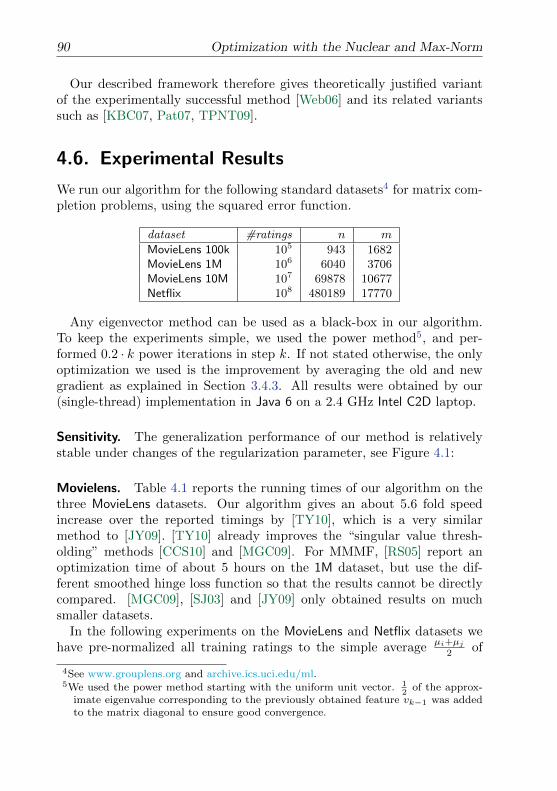
90 Optimization with the Nuclear and Max-Norm
Our described framework therefore gives theoretically justified variantof the experimentally successful method [Web06] and its related variantssuch as [KBC07, Pat07, TPNT09].
4.6. Experimental Results
We run our algorithm for the following standard datasets4 for matrix com-pletion problems, using the squared error function.
dataset #ratings n m
MovieLens 100k 105 943 1682MovieLens 1M 106 6040 3706MovieLens 10M 107 69878 10677Netflix 108 480189 17770
Any eigenvector method can be used as a black-box in our algorithm.To keep the experiments simple, we used the power method5, and per-formed 0.2 · k power iterations in step k. If not stated otherwise, the onlyoptimization we used is the improvement by averaging the old and newgradient as explained in Section 3.4.3. All results were obtained by our(single-thread) implementation in Java 6 on a 2.4 GHz Intel C2D laptop.
Sensitivity. The generalization performance of our method is relativelystable under changes of the regularization parameter, see Figure 4.1:
Movielens. Table 4.1 reports the running times of our algorithm on thethree MovieLens datasets. Our algorithm gives an about 5.6 fold speedincrease over the reported timings by [TY10], which is a very similarmethod to [JY09]. [TY10] already improves the “singular value thresh-olding” methods [CCS10] and [MGC09]. For MMMF, [RS05] report anoptimization time of about 5 hours on the 1M dataset, but use the dif-ferent smoothed hinge loss function so that the results cannot be directlycompared. [MGC09], [SJ03] and [JY09] only obtained results on muchsmaller datasets.
In the following experiments on the MovieLens and Netflix datasets wehave pre-normalized all training ratings to the simple average
µi+µj2 of
4See www.grouplens.org and archive.ics.uci.edu/ml.5We used the power method starting with the uniform unit vector. 1
2of the approx-
imate eigenvalue corresponding to the previously obtained feature vk−1 was addedto the matrix diagonal to ensure good convergence.
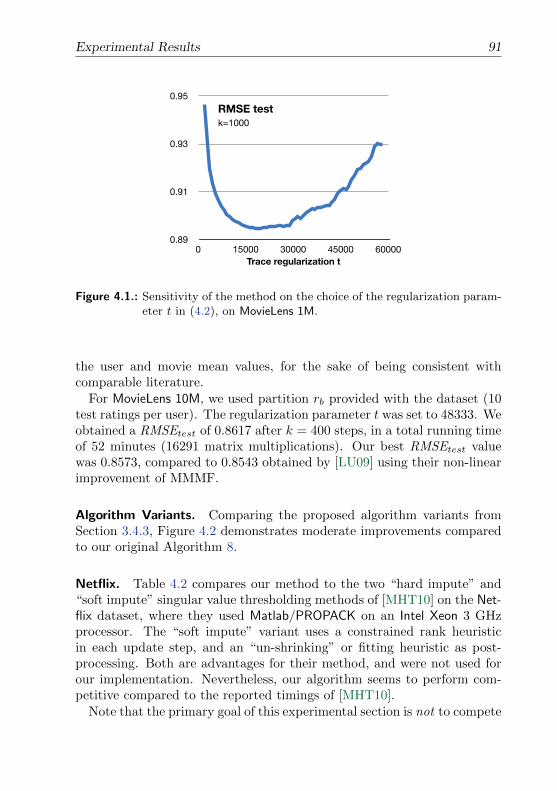
Experimental Results 91
0.89
0.91
0.93
0.95
0 15000 30000 45000 60000Trace regularization t
RMSE testk=1000
Figure 4.1.: Sensitivity of the method on the choice of the regularization param-eter t in (4.2), on MovieLens 1M.
the user and movie mean values, for the sake of being consistent withcomparable literature.
For MovieLens 10M, we used partition rb provided with the dataset (10test ratings per user). The regularization parameter t was set to 48333. Weobtained a RMSEtest of 0.8617 after k = 400 steps, in a total running timeof 52 minutes (16291 matrix multiplications). Our best RMSEtest valuewas 0.8573, compared to 0.8543 obtained by [LU09] using their non-linearimprovement of MMMF.
Algorithm Variants. Comparing the proposed algorithm variants fromSection 3.4.3, Figure 4.2 demonstrates moderate improvements comparedto our original Algorithm 8.
Netflix. Table 4.2 compares our method to the two “hard impute” and“soft impute” singular value thresholding methods of [MHT10] on the Net-flix dataset, where they used Matlab/PROPACK on an Intel Xeon 3 GHzprocessor. The “soft impute” variant uses a constrained rank heuristicin each update step, and an “un-shrinking” or fitting heuristic as post-processing. Both are advantages for their method, and were not used forour implementation. Nevertheless, our algorithm seems to perform com-petitive compared to the reported timings of [MHT10].
Note that the primary goal of this experimental section is not to compete
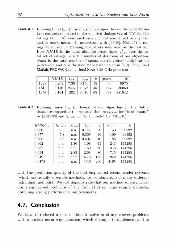
92 Optimization with the Nuclear and Max-Norm
Table 4.1.: Running times tour (in seconds) of our algorithm on the three Movie-Lens datasets compared to the reported timings tTY of [TY10]. Theratings 1, . . . , 5 were used as-is and not normalized to any userand/or movie means. In accordance with [TY10], 50% of the rat-ings were used for training, the others were used as the test set.Here NMAE is the mean absolute error, times 1
5−1, over the to-
tal set of ratings. k is the number of iterations of our algorithm,#mm is the total number of sparse matrix-vector multiplicationsperformed, and tr is the used trace parameter t in (4.2). They usedMatlab/PROPACK on an Intel Xeon 3.20 GHz processor.
NMAE tTY tour k #mm tr
100k 0.205 7.39 0.156 15 33 99751M 0.176 24.5 1.376 35 147 3606010M 0.164 202 36.10 65 468 281942
Table 4.2.: Running times tour (in hours) of our algorithm on the Netflixdataset compared to the reported timings tM,hard for “hard impute”by [MHT09] and tM,soft for “soft impute” by [MHT10].
RMSEtest tM,hard tM,soft tour k #mm tr
0.986 3.3 n.a. 0.144 20 50 995920.977 5.8 n.a. 0.306 30 109 995920.965 6.6 n.a. 0.504 40 185 995920.962 n.a. 1.36 1.08 45 243 1742850.957 n.a. 2.21 1.69 60 416 1742850.954 n.a. 2.83 2.68 80 715 1742850.9497 n.a. 3.27 6.73 135 1942 1742850.9478 n.a. n.a. 13.6 200 4165 174285
with the prediction quality of the best engineered recommender systems(which are usually ensemble methods, i.e. combinations of many differentindividual methods). We just demonstrate that our method solves nuclearnorm regularized problems of the form (4.2) on large sample datasets,obtaining strong performance improvements.
4.7. Conclusion
We have introduced a new method to solve arbitrary convex problemswith a nuclear norm regularization, which is simple to implement and to
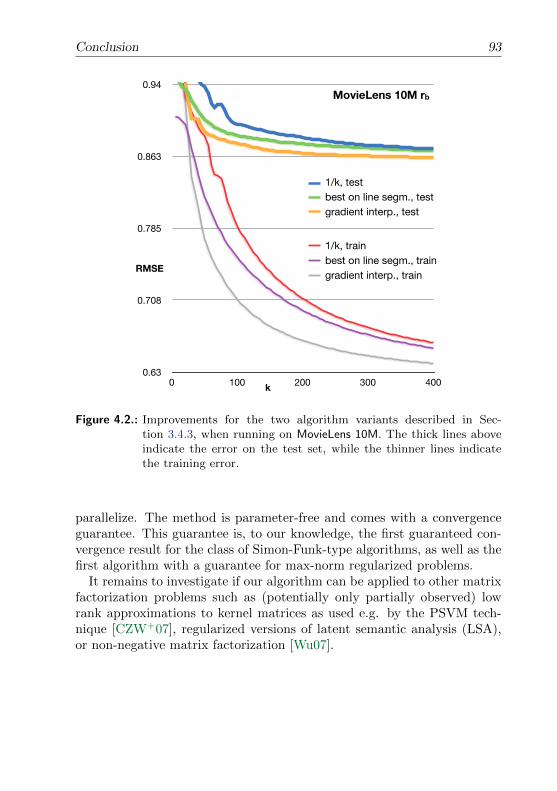
Conclusion 93
0.63
0.708
0.785
0.863
0.94
0 100 200 300 400k
RMSE
MovieLens 10M rb
1/k, test
best on line segm., test
gradient interp., test
1/k, train
best on line segm., train
gradient interp., train
Figure 4.2.: Improvements for the two algorithm variants described in Sec-tion 3.4.3, when running on MovieLens 10M. The thick lines aboveindicate the error on the test set, while the thinner lines indicatethe training error.
parallelize. The method is parameter-free and comes with a convergenceguarantee. This guarantee is, to our knowledge, the first guaranteed con-vergence result for the class of Simon-Funk-type algorithms, as well as thefirst algorithm with a guarantee for max-norm regularized problems.
It remains to investigate if our algorithm can be applied to other matrixfactorization problems such as (potentially only partially observed) lowrank approximations to kernel matrices as used e.g. by the PSVM tech-nique [CZW+07], regularized versions of latent semantic analysis (LSA),or non-negative matrix factorization [Wu07].

5A Geometric OptimizationMethod, and Coresets for
Polytope Distance andSVMs
In this chapter, we translate the coreset framework to the problems of find-ing the point closest to the origin inside a polytope, finding the shortest dis-tance between two polytopes, Perceptrons, and soft- as well as hard-marginSupport Vector Machines (SVM). To do so, we will study a geometricequivalent of Clarkson’s optimization approach over the simplex [Cla10],which we have described in Chapters 2 and 3.
We prove asymptotically matching upper and lower bounds on the sizeof coresets, stating that ε-coresets of size d(1 + o(1))E∗/εe do always existas ε → 0, and that this is optimal. The crucial quantity E∗ is what wecall the excentricity of a polytope, or a pair of polytopes, correspondingto the curvature constant in the general convex optimization setting inChapter 2.
Additionally, we prove linear convergence speed of Gilbert’s algorithm,one of the earliest known approximation algorithms for polytope distance,and generalize both the algorithm and the proof to the two polytope case.
95
96A Geometric Optimization Method, and Coresets for Polytope Distance
and SVMs
Interestingly, our coreset bounds also imply that we can for the firsttime prove asymptotically matching upper and lower bounds for the spar-sity of Perceptron and SVM solutions (which in this case is the number ofsupport vectors), as a function of the approximation quality.
This chapter is based on the paper [GJ09] with Bernd Gartner.
5.1. Introduction
Coresets. The concept of coresets has proven to be a very successful onefor approximation algorithms for many discrete geometric problems. Onone hand coreset algorithms are much faster than exact algorithms, and onthe other hand they simultaneously ensure that the obtained approximatesolutions still have very compact (sparse) representations, making themvery appealing for many practical applications e.g. in machine learning.
Originally introduced for smallest enclosing ball problem and clusteringby [BHPI02], and for extent measures by [APV02], the idea of a coreset isthe following: instead of solving the original problem, one tries to identifya very small subset (coreset) of the points, such that the solution just onthe coreset is guaranteed to be a good approximation of the true solutionto the original problem. For the problem of finding the smallest enclosingball of n points P ∈ Rd, and ε > 0, an ε-coreset S is a small subset ofthe points P such that the smallest enclosing ball of just S, blown up by afactor of 1 + ε, contains all the original points P . It was shown that hereε-coresets of size d1/εe do always exist [BC03, BC07] and that this is bestpossible [BC07]. This is very remarkable because the size of the coresetis independent of the dimension d of the space, and also independent ofthe number of points n, making it very attractive for the use in large scaleproblems (high n) and kernel methods (high d). This nice property isin contrast to many other geometric problems for which coresets usuallyhave size exponential in the dimension, e.g. Θ(1/ε(d−1)/2) for the extentproblem [AHPV04]. For a nice review on existing coreset algorithms werefer to [AHPV05].
Clarkson in [Cla10] significantly widened the class of problems where thecoreset idea can be applied, and showed that the nice property of constantO(1/ε) sized coresets indeed holds for the general problem of minimizing aconvex function over the unit simplex. In the previous Chapter 2, we havegeneralized this coreset technique to optimizing over arbitrary compactdomains, and have obtained matching lower bounds on the coreset size for
Introduction 97
the simplex as well as for general `1-regularized convex problems.
Our Contributions and Related Work. Following the approach of [Cla10],we translate the coreset framework to the polytope distance problem of onepolytope (w.r.t. the origin), distance between two polytopes, and hard- aswell as soft-margin support vector machines, and introduce the geometricmeaning of coresets and strong primal-dual approximation in this context.
We prove a new lower bound of⌈E∗
ε
⌉+ 1 for the size of ε-coresets
for polytope distance, where E∗ is what we call the excentricity of the
polytope. Together with the upper bound of⌈E∗(1+o(1))
ε
⌉as ε → 0, this
shows that the size of the obtained ε-coresets is asymptotically optimal.We also show tight bounds (up to a factor of two) for the distance problembetween two polytopes.
For Gilbert’s algorithm [Gil66], one of the earliest known approximationalgorithms for polytope distance, we give the first two proofs of convergencespeed: First by observing that is in fact just an instance of the FrankWolfe approximation algorithm for quadratic programs [FW56], which isnow often called sparse greedy approximation, and secondly by giving aslightly easier geometric interpretation of the analytic proof of [Cla10].Also, we generalize Gilbert’s algorithm to the distance problem betweentwo polytopes, where we are able to prove the same convergence speed.Furthermore, we can get rid of the expensive search for a starting pointin this case which in previous approaches needed time quadratic in thenumber of points [Roo00, VSM03].
Applications to Machine Learning. On the application side, it is our goalto apply concepts and algorithms from computational geometry to machinelearning. Support Vector Machines (SVM) [BGV92, CV95, Bur98] areamong the most established and successful classification tools in machinelearning, where from the name it is not immediately clear that the conceptrefers to nothing else than the separation of two classes of points by ahyperplane, with the largest possible margin. From the formulation as aquadratic program it follows that the problem is equivalent to the polytopedistance problem, either for one or for two polytopes, depending on whichSVM variant is considered (See Section 5.5). The Perceptron [Ros58] refersto the case where we search for any hyperplane that separates two pointclasses, not necessarily one of maximum margin. The term kernel methodssummarizes SVMs and Perceptrons where the points are assumed to livein an implicit high-dimensional feature space where we just know their
98A Geometric Optimization Method, and Coresets for Polytope Distance
and SVMs
pairwise scalar-products which is then called the kernel.
Sparsity of solutions. Our main contribution is to relate the coreset con-cept to sparsity of solutions of kernel methods: Using our bounds for thesize of coresets, we derive a new fundamental property of SVMs and Per-ceptrons, giving nearly matching upper and lower bounds on the sparsityof their solutions, a parameter which is absolutely crucial for the practi-cal performance of these methods on large scale problems. More preciselywe show that any solution for a SVM or Perceptron, attaining at least a
fraction µ of the optimal margin, must have at least⌈E∗
1−µ
⌉+ 1 many (or⌈
12E∗
1−µ
⌉+2 in the two class case) non-zero coefficients in the worst case, and
that a solution with⌈E∗(1+o(1))
1−µ
⌉many non-zero coefficients can always be
obtained for all instances. We are not aware of any existing lower boundson the sparsity in the literature.
Training SVM in linear time. For any fixed fraction 0 ≤ µ < 1, we showthat Gilbert’s algorithm in time O(n) finds a solution attaining at least aµ-fraction of the optimal margin to the SVM and Perceptron (no matter ifa kernel is used or not). This guarantee contrasts most of the existing SVMtraining algorithms which run in time usually cubic in n, or then often haveno theoretical approximation guarantees except from converging in a finitenumber of steps [Pla99], or have guarantees only on the primal or dual ob-jective value, but not both. Tsang et al. have already applied the smallestenclosing ball coreset approach to train SVMs under the name Core VectorMachine (CVM) [TKC05, TKK07], for one particular SVM variant (`2-losswith regularized offset), in the case that all points have the same norm.In this case the smallest enclosing ball problem is equivalent to findingthe distance of one polytope from the origin. In another work [HPRZ07]directly used coresets to solve the problem of separating two polytopes bya hyperplane passing through the origin, but this is again equivalent to aone polytope distance problem. Both approaches are therefore generalizedby [Cla10] and this work, proving faster algorithm convergence and smallercoresets. Here we generalize the coreset methods further to the two poly-tope case, encompassing all the currently most used hard- and soft-marginSVM variants with arbitrary kernels, with both `1 and `2-loss, in particu-lar the special case of the CVM [TKC05, TKZ06, TKK07] and [HPRZ07],while obtaining faster convergence and smaller coresets. Our generaliza-tion shows that all of the mostly used SVM variants can be trained in time
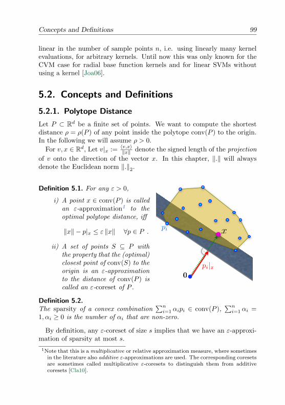
Concepts and Definitions 99
linear in the number of sample points n, i.e. using linearly many kernelevaluations, for arbitrary kernels. Until now this was only known for theCVM case for radial base function kernels and for linear SVMs withoutusing a kernel [Joa06].
5.2. Concepts and Definitions
5.2.1. Polytope Distance
Let P ⊂ Rd be a finite set of points. We want to compute the shortestdistance ρ = ρ(P ) of any point inside the polytope conv(P ) to the origin.In the following we will assume ρ > 0.
For v, x ∈ Rd, Let v|x := 〈v,x〉‖x‖ denote the signed length of the projection
of v onto the direction of the vector x. In this chapter, ‖.‖ will alwaysdenote the Euclidean norm ‖.‖2.
pi
0
pi|x
x
Definition 5.1. For any ε > 0,
i) A point x ∈ conv(P ) is calledan ε-approximation1 to theoptimal polytope distance, iff
‖x‖ − p|x ≤ ε ‖x‖ ∀p ∈ P .
ii) A set of points S ⊆ P withthe property that the (optimal)closest point of conv(S) to theorigin is an ε-approximationto the distance of conv(P ) iscalled an ε-coreset of P .
Definition 5.2.The sparsity of a convex combination
∑ni=1 αipi ∈ conv(P ),
∑ni=1 αi =
1, αi ≥ 0 is the number of αi that are non-zero.
By definition, any ε-coreset of size s implies that we have an ε-approxi-mation of sparsity at most s.
1Note that this is a multiplicative or relative approximation measure, where sometimesin the literature also additive ε-approximations are used. The corresponding coresetsare sometimes called multiplicative ε-coresets to distinguish them from additivecoresets [Cla10].
100A Geometric Optimization Method, and Coresets for Polytope Distance
and SVMs
The Duality Gap as a Certificate of Approximation Quality. Beingan ε-approximation can be interpreted as the multiplicative gap betweenthe “primal” distance f(x) = ‖x‖, and the corresponding “dual” valueω(x) = min
p∈Pp|x, being small, analogously to our concept of the “poor-
man’s” duality as described in Section 2.2. We will explain this connectionin more detail in Section 5.2.3 below.
Also, the weak-duality observation (2.6), as we have seen for our generalconvex optimization setting from Section 2.2 has a clear geometric meaninghere: Our geometric definition of an approximation automatically impliesthat the current distance ‖x‖ must already be close to the (unknown)optimal value ρ, i.e.
Lemma 5.3. If x is an ε-approximation, then (1− ε) ‖x‖ ≤ ρ ≤ ‖x‖ .Proof. RHS: Clear by definition of the distance ρ. LHS: By definition of anε-approximation, we have a closed halfspace (normal to x), with distance(1− ε) ‖x‖ from the origin, which contains conv(P ), which itself containsthe optimal point x∗ with ‖x∗‖ = ρ.
Excentricity and Curvature.
Definition 5.4. We define the excentricity of a point set P as E := D2
ρ2 ,
where D := maxp,q∈P ‖p− q‖ is the diameter of the polytope and ρ is thetrue polytope distance to the origin.
Also, we define the asymptotic excentricity E∗ := R2
ρ2 , where we call
R := maxp∈P ‖p− c‖ the radius of the polytope. Here c is the unique2
point attaining the minimum distance ρ to the origin.
It immediately follows that E∗ ≤ E ≤ 4E∗ by triangle inequality (R ≤D ≤ 2R).
Also, the quantities E and E∗ do indeed correspond to the curvatureor “non-linearity” introduced by [Cla10], that we studied in Section 2.3.4.We will explain this correspondence in the following Section 5.2.3.
5.2.2. Distance Between Two Polytopes
It is easy to see that the problem of finding the shortest distance betweentwo polytopes is equivalent to finding the shortest vector in a single poly-
2We note that the point c attaining the optimal distance minp∈P ‖p‖ of the polytopeto the origin is always unique: Assume there would be two distinct points c1, c2attaining the minimum, then their mid-point 1
2(c1 + c2) would have even shorter
distance to the origin, contradicting the assumption of optimality of c1.
Concepts and Definitions 101
tope, their Minkowski difference:
Definition 5.5. The Minkowski difference
MD(P1, P2) := u− v |u ∈ conv(P1), v ∈ conv(P2)of two polytopes conv(P1) and conv(P2) is the set (in fact it is also apolytope [Zie95]) consisting of all difference vectors.
Observe that conv(P1) and conv(P2) are separable by a hyperplane iff0 /∈ MD(P1, P2). We call a vector x = x1 − x2 an ε-approximation for thedistance problem between the two polytopes conv(P1) and conv(P2) iff xis an ε-approximation for MD(P1, P2). By the sparsity of a convex combi-nation in MD(P1, P2) we always mean the minimum number of non-zerocoefficients of a representation as a difference of two convex combinationsin the original polytopes. An ε-coreset is a subset P ′1 ∪ P ′2 of the twooriginal point sets, P ′1 ⊆ P1, P
′2 ⊆ P2, such that the shortest vector in the
restricted Minkowski difference MD(P ′1, P′2) is an ε-approximation.
Definition 5.6. We define the excentricity of a pair of two polytopes as
EP1,P2:= (D1+D2)2
ρ2 and the asymptotic excentricity as E∗P1,P2:= (R1+R2)2
ρ2 ,
with Dk, Rk denoting diameter and radius3, ρ being the true distance be-tween the two polytopes.
Interpreting this excentricity in comparison to the equivalent single poly-tope problem given by the Minkowski difference, it is easy to see thatEMD(P1,P2) ≤ EP1,P2
, since diam(MD(P1, P2)) ≤ diam(P1) + diam(P2).
Alternatively, for comparison, we can also write EP1,P2= (D1+D2)2
ρ2 =(√E1 +
√E2
)2and E∗P1,P2
=(√
E∗1 +√E∗2)2
if we think of the Ek, E∗k are
being the “individual” excentricities of each polytope conv(Pk), k = 1, 2,here with respect to the corresponding closest point in the other polytope(if the closest pair is unique).
5.2.3. Relation to our General Setting of ConvexOptimization Over Bounded Domain
Duality. Comparing the above geometric concept of approximation to ourgeneral optimization framework from Chapter 2, we observe that there isindeed a direct correspondence:
3Here the radius Rk is with respect to the corresponding endpoint of the optimal pairattaining the closest distance between the two polytopes. When using E∗P1,P2
, wewill assume that the optimal pair is unique.
102A Geometric Optimization Method, and Coresets for Polytope Distance
and SVMs
For the choice of convex objective function f(x) := ‖x‖, the gradientis given by ∇f(x) = x
‖x‖ for any x 6= 0. Therefore, the corresponding
“poor-man’s” dual value for each point x as given in equation (2.4) is infact exactly the same geometric quantity as used in Definition 5.1,
ω(x) = minp∈P‖x‖+ (p− x)T
x
‖x‖= min
p∈PpT
x
‖x‖= min
p∈Pp|x .
Alternatively, one can also reduce the polytope distance problem toconvex optimization over the simplex, as in Clarkson’s framework [Cla10],by using barycentric coordinates, see also Section 3.1. In this case, thecorresponding convex objective function is f(x) := ‖Ax‖, where A ∈ Rd×nis the matrix containing all points of P as columns.
Curvature. The above defined excentricity and the more general curva-ture constant Cf of a convex function are in fact closely related.
Lemma 5.7. For the objective function f(x) := ‖x‖ over the domain D =conv(P ), the curvature of f is bounded by the excentricity as follows.
Cf ≤ρ
2E and C∗f ≤
ρ
2E∗ .
Proof. Using that ∇f(x) = x‖x‖ for any x 6= 0, we can consider the Hessian
matrix (∇2f(x))ij = ∂f(x)∂xi∂xj
, and calculate
∇2f(x) =I
‖x‖ −xxT
‖x‖3.
Here I is the n×n identity matrix. Plugging this expression into the upperbound for the curvature Cf as given by inequality (2.12) from Section 2.3.4,we obtain
Cf ≤ supx,y∈D,
z∈[x,y]⊆D
12 (y − x)T
(I‖z‖ − zzT
‖z‖3)
(y − x)
= supx,y∈D,
z∈[x,y]⊆D
12
(‖y−x‖2‖z‖ − (y−x)T zzT (y−x)
‖z‖3)
= supx,y∈D,
z∈[x,y]⊆D
12
(‖y−x‖2−((y−x)|z)2
‖z‖
)
Lower Bounds on the Sparsity of ε-Approximations 103
To obtain the middle equality, we have just rewritten the second term(y−x)T zzT (y−x)
‖z‖3 =‖(y−x)T z
‖z‖‖2‖z‖ = ((y−x)|z)2
‖z‖ using the definition of the
projection v|z.The desired upper bound Cf ≤ ρ
2E = D2
2ρ now directly follows from justignoring the negative term in the above expression of the supremum.
Analogously, when using the definition (2.11) of the asymptotic curva-ture C∗f , together with the fact that the closest point x∗ is the uniqueoptimum, we have that
C∗f ≤ supy∈D,
z∈[x∗,y]⊆D
12
(‖y−x∗‖2−((y−x∗)|z)2
‖z‖
),
for which again ignoring the projection term, the optimum choice of z := x∗
will result in the bound C∗f ≤ ρ2E∗ = R2
2ρ .
5.3. Lower Bounds on the Sparsity ofε-Approximations
In this Section we will give two constructions of point sets, such that nosmall ε-coresets can possibly exist for the polytope distance problem. Thegeometric interpretation of these constructions is in fact very simple:
5.3.1. Distance of One Polytope from the Origin
Warm-Up. Consider the (d−1)-simplex spanned by P being the set of thed standard unit vectors in Rd, but imagine the simplex being just slightlyblown up (scaled linearly) from its barycenter c. Then the projection ofany point pi ∈ P onto any convex combination x of some of the otherpoints becomes negative, implying that no ε-coresets of size < d (andalso no ε-approximations of sparsity < d ) can exist for any ε ≤ 1. Wewill make this more formal in the following lemma. The unit simplex hasD =
√2 and ρ = 1√
dso the excentricity of our polytope conv(P ) is roughly
E = 2d, or E∗ = d − 1 respectively. In the following we will see that thequantities 1
2E and E∗ + 1 can indeed be turned into lower bounds on thesize of ε-coresets and the sparsity of ε-approximations, in terms of theapproximation quality ε. The following lemma explains the construction:
Lemma 5.8. For any given 0 < ε < 1, and for any d ≥ 2, there exists aset of d points P ⊂ Rd, such that
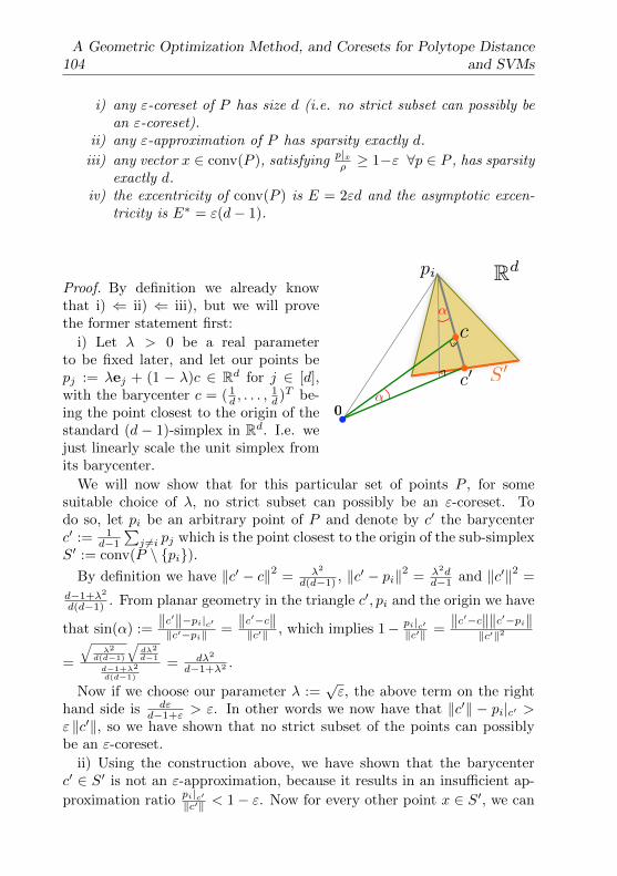
104A Geometric Optimization Method, and Coresets for Polytope Distance
and SVMs
i) any ε-coreset of P has size d (i.e. no strict subset can possibly bean ε-coreset).
ii) any ε-approximation of P has sparsity exactly d.
iii) any vector x ∈ conv(P ), satisfying p|xρ ≥ 1−ε ∀p ∈ P , has sparsity
exactly d.iv) the excentricity of conv(P ) is E = 2εd and the asymptotic excen-
tricity is E∗ = ε(d− 1).
pi
α
α
Rd
c
c′ S′
0
Proof. By definition we already knowthat i) ⇐ ii) ⇐ iii), but we will provethe former statement first:
i) Let λ > 0 be a real parameterto be fixed later, and let our points bepj := λej + (1 − λ)c ∈ Rd for j ∈ [d],with the barycenter c = ( 1
d , . . . ,1d )T be-
ing the point closest to the origin of thestandard (d − 1)-simplex in Rd. I.e. wejust linearly scale the unit simplex fromits barycenter.
We will now show that for this particular set of points P , for somesuitable choice of λ, no strict subset can possibly be an ε-coreset. Todo so, let pi be an arbitrary point of P and denote by c′ the barycenterc′ := 1
d−1
∑j 6=i pj which is the point closest to the origin of the sub-simplex
S′ := conv(P \ pi).By definition we have ‖c′ − c‖2 = λ2
d(d−1) , ‖c′ − pi‖2 = λ2dd−1 and ‖c′‖2 =
d−1+λ2
d(d−1) . From planar geometry in the triangle c′, pi and the origin we have
that sin(α) :=‖c′‖−pi|c′‖c′−pi‖ =
‖c′−c‖‖c′‖ , which implies 1− pi|c′
‖c′‖ =‖c′−c‖‖c′−pi‖
‖c′‖2
=
√λ2
d(d−1)
√dλ2
d−1
d−1+λ2
d(d−1)
= dλ2
d−1+λ2 .
Now if we choose our parameter λ :=√ε, the above term on the right
hand side is dεd−1+ε > ε. In other words we now have that ‖c′‖ − pi|c′ >
ε ‖c′‖, so we have shown that no strict subset of the points can possiblybe an ε-coreset.
ii) Using the construction above, we have shown that the barycenterc′ ∈ S′ is not an ε-approximation, because it results in an insufficient ap-
proximation ratio pi|c′‖c′‖ < 1− ε. Now for every other point x ∈ S′, we can
Lower Bounds on the Sparsity of ε-Approximations 105
show that the ratio becomes even worse, if we argue as follows: In the de-nominator we know that c′ is the point in S′ of minimum norm, and in thenumerator it holds that pi|c′ ≥ pi|x ∀x ∈ S′. The last inequality followsfrom the fact that the distance of a point x to a linear space is always atmost as large as the distance to a subspace of it — or more formally if p(x),p(c′) are the two projections of pi onto x and c′ respectively, we get that∥∥pi − p(x)
∥∥ ≥ ∥∥∥pi − p(c′)∥∥∥ since x ∈ lin(S′) and pi|c′ =
∥∥∥p(c′)∥∥∥ = pi|lin(S′).
But by the Pythagorean theorem this implies pi|x ≤ pi|c′ . We have shownthat no ε-approximation of sparsity < d can possibly exist for our givenpoint set.
iii) Let again λ2 := ε, and suppose x ∈ S′ = conv(P \pi) for some pi ∈P is such a convex combination of sparsity ≤ d−1. We use the above result
and calculate pi|xρ ≤
pi|c′ρ = ‖c′‖ (1− dε
d−1+ε )√d =
√d−1+εd(d−1)
(d−1)(1−ε)d−1+ε
√d =√
d−1d−1+ε (1− ε) < 1− ε.iv) It is straightforward to calculate that our point set has diameterD2 =
‖p1 − p2‖2 = 2λ2, radius R2 = λ2 d−1d , and true distance ρ2 = ‖c‖2 = 1
d ,so for the excentricity we obtain E = 2εd and E∗ = ε(d− 1).
Theorem 5.9. For any given 0 < ε < 1, for any d ≥ 2, there exists a setof d points P ⊂ Rd, such that the sparsity of any ε-approximation, and thesize of any ε-coreset of P is at least⌈ 1
2E
ε
⌉and
⌈E∗
ε
⌉+ 1
Proof. The point set P from Lemma 5.8 satisfies12E
ε = d, and E∗
ε =d− 1.
Note that the bound using E is by a factor of 2 better than if we wouldjust have used the trivial bound E ≤ 4E∗ together with the result for E∗.
5.3.2. Distance Between Two Polytopes
Observation 5.10. If we have two point sets, one consisting of just onepoint and the other consisting of d points, and we consider the polytopedistance problem between the corresponding two polytopes, the lower boundof Lemma 5.8 directly applies to the Minkowski difference, resulting in the
lower bounds⌈
12E
ε
⌉+ 1 and
⌈E∗
ε
⌉+ 2 because we always need the single
point of the second class in any linear combination. In this case the pair
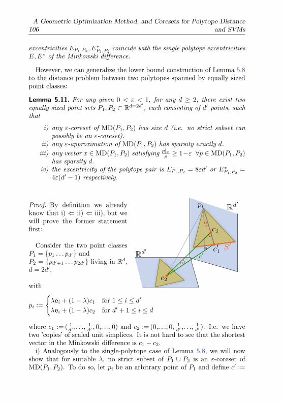
106A Geometric Optimization Method, and Coresets for Polytope Distance
and SVMs
excentricities EP1,P2, E∗P1,P2
coincide with the single polytope excentricitiesE,E∗ of the Minkowski difference.
However, we can generalize the lower bound construction of Lemma 5.8to the distance problem between two polytopes spanned by equally sizedpoint classes:
Lemma 5.11. For any given 0 < ε < 1, for any d ≥ 2, there exist twoequally sized point sets P1, P2 ⊂ Rd=2d′ , each consisting of d′ points, suchthat
i) any ε-coreset of MD(P1, P2) has size d (i.e. no strict subset canpossibly be an ε-coreset).
ii) any ε-approximation of MD(P1, P2) has sparsity exactly d.
iii) any vector x ∈ MD(P1, P2) satisfying p|xρ ≥ 1−ε ∀p ∈ MD(P1, P2)
has sparsity d.iv) the excentricity of the polytope pair is EP1,P2 = 8εd′ or E∗P1,P2
=4ε(d′ − 1) respectively.
Rd′
Rd′
c2
c1
c′1
pi
α
αc′
S′
Proof. By definition we alreadyknow that i) ⇐ ii) ⇐ iii), but wewill prove the former statementfirst:
Consider the two point classesP1 = p1 . . . pd′ andP2 = pd′+1 . . . p2d′ living in Rd,d = 2d′,
with
pi :=
λei + (1− λ)c1 for 1 ≤ i ≤ d′λei + (1− λ)c2 for d′ + 1 ≤ i ≤ d
where c1 := ( 1d′ ,. . .,
1d′ , 0,. . ., 0) and c2 := (0,. . ., 0, 1
d′ ,. . .,1d′ ). I.e. we have
two ’copies’ of scaled unit simplices. It is not hard to see that the shortestvector in the Minkowski difference is c1 − c2.
i) Analogously to the single-polytope case of Lemma 5.8, we will nowshow that for suitable λ, no strict subset of P1 ∪ P2 is an ε-coreset ofMD(P1, P2). To do so, let pi be an arbitrary point of P1 and define c′ :=
Lower Bounds on the Sparsity of ε-Approximations 107
c′1 − c2 where the barycenter c′1 := 1d′−1
∑j 6=i pj is the point of the sub-
simplex S′ := conv(P1 \ pi) closest to c2. It is easy to check that c′ isindeed the new shortest distance after removal of pi.
By definition we have ‖c′1 − c1‖2 = λ2
d′(d′−1) , ‖c′1 − pi‖2 = λ2d′
d′−1 and
‖c′‖2 = 2(d′−1)+λ2
d′(d′−1) . From planar geometry in the triangle c′1, pi and c2 we
again have that
sin(α) :=‖c′‖−(pi−c2)|c′‖c′1−pi‖ =
‖c′1−c1‖‖c′‖ , which implies 1− (pi−c2)|c′
‖c′‖
=‖c′1−c1‖‖c′1−pi‖
‖c′‖2 =
√λ2
d′(d′−1)
√d′λ2d′−1
2(d′−1)+λ2
d′(d′−1)
= d′λ2
2(d′−1)+λ2 .
Now if we choose our parameter λ :=√
2ε, the above term on the righthand side is d′2ε
2(d′−1)+2ε > ε. In other words we now have that ‖c′‖ − (pi −c2)|c′ > ε ‖c′‖, so we have shown that no strict subset of the 2d′ points canpossibly be an ε-coreset.
ii) The argument that the approximation ratio p|x‖x‖ is indeed best for the
distance vector x := c′ — and thus there really is no ε-approximation ofsparsity < d — is the same as in the proof of Lemma 5.8, and additionallyusing that (pi − y2)|c′ = (pi − c2)|c′ ∀y2 ∈ conv(P2), as c′ is orthogonalon conv(P2).
iii) Let again λ2 := 2ε, and suppose x ∈ S′ = conv(P1 \ pi) for somepi ∈ P1 is such a convex combination of sparsity ≤ d−1. We use the above
result and calculate (pi−c2)|xρ ≤ (pi−c2)|c′
ρ = ‖c′‖ (1− d′2ε2(d′−1)+2ε )
√d′2
=√
2(d′−1)+2εd′(d′−1)
(d′−1)(1−ε)d′−1+ε
√d′2 =
√d′−1d′−1+ε (1− ε) < 1− ε.
iv) Check that each of our two polytopes has diameter D2 = 2λ2 and
radius R2 = λ2 d′−1d′ . Since the optimal distance ρ2 = 2
d′ , it follows that the
pair excentricity is EP1,P2= (√
2λ+√
2λ)2
2/d′ = 8λ2
2/d′ = 8εd′ and the asymptotic
pair excentricity is E∗P1,P2=
(√d′−1d′ λ+
√d′−1d′ λ
)2
2/d′ =4 d′−1d′ λ
2
2/d′ = 4ε(d′ −1).
Theorem 5.12. For any given 0 < ε < 1, for any d ≥ 2, there exist twoequally sized point sets P1, P2 ⊂ Rd=2d′ , each consisting of d′ points, suchthat the sparsity of any ε-approximation of MD(P1, P2), and the size ofany ε-coreset is at least⌈ 1
4EP1,P2
ε
⌉and
⌈12E∗P1,P2
ε
⌉+ 2 .
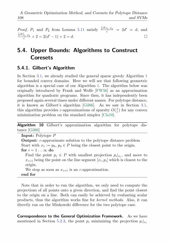
108A Geometric Optimization Method, and Coresets for Polytope Distance
and SVMs
Proof. P1 and P2 from Lemma 5.11 satisfy14EP1,P2
ε = 2d′ = d, and12E∗P1,P2
ε + 2 = 2(d′ − 1) + 2 = d.
5.4. Upper Bounds: Algorithms to ConstructCoresets
5.4.1. Gilbert’s Algorithm
In Section 3.1, we already studied the general sparse greedy Algorithm 1for bounded convex domains. Here we will see that following geometricalgorithm is a special case of our Algorithm 1. The algorithm below wasoriginally introduced by Frank and Wolfe [FW56] as an approximationalgorithm for quadratic programs. Since then, it has independently beenproposed again several times under different names. For polytope distance,it is known as Gilbert’s algorithm [Gil66]. As we saw in Section 3.1,this algorithm provides ε-approximations of sparsity O( 1
ε ) for any convexminimization problem on the standard simplex [Cla10].
Algorithm 10 Gilbert’s approximation algorithm for polytope dis-tance [Gil66]
Input: Polytope POutput: ε-approximate solution to the polytope distance problemStart with x1 := p0, p0 ∈ P being the closest point to the origin.for i = 1 . . .∞ do
Find the point pi ∈ P with smallest projection pi|xi , and move toxi+1 being the point on the line segment [xi, pi] which is closest to theorigin.We stop as soon as xi+1 is an ε-approximation.
end for
Note that in order to run the algorithm, we only need to compute theprojections of all points onto a given direction, and find the point closestto the origin on a line. Both can easily be achieved by evaluating scalarproducts, thus the algorithm works fine for kernel methods. Also, it candirectly run on the Minkowski difference for the two polytope case.
Correspondence to the General Optimization Framework. As we havementioned in Section 5.2.3, the point pi minimizing the projection pi|xi
Upper Bounds: Algorithms to Construct Coresets 109
(which is then used as the step-direction in the above Algorithm 10) isexactly a solution to the linearized problem ExactLinear (∇f(xi), D),for the convex function f(x) := ‖x‖ over the domain D = conv(P ). Thismeans that Algorithm 10 in fact coincides with the general line-searchAlgorithm 2 for this choice of objective function and domain.
Variants and applications. Gilbert’s geometric algorithm has been ap-plied to SVM training in the case of hard-margin as well as soft-marginwith both `2-loss [KSBM00] and `1-loss [MST06, MT06]4. A variant ofGilbert’s algorithm, the GJK algorithm, is one of the most popular algo-rithm for collision detection in 3 dimensional space [GJK88]. For SVMtraining, Gilbert’s algorithm was recently also implemented on FPGAhardware [PB08].
Another important variant of this, called the MDM algorithm [MDM74],is in fact equivalent to one of the most used SVM training algorithms,SMO [Pla99, LBD08]. For SVM training, [KSBM00] obtained good exper-imental results with a combination of Gilbert’s and the MDM algorithm.
Convergence speed and running time. All mentioned algorithms in theabove paragraph have in common that they converge, were successfullyapplied in practice, but no convergence speed or bound on the runningtime has ever been proved so far. Here we prove the convergence speed forGilbert’s algorithm, on one hand by observing for the first time that it isnothing else than the Frank-Wolfe algorithm [FW56] applied to the stan-dard quadratic programming formulation of polytope distance5, and onthe other hand by giving a new slightly easier geometric variant of recentproofs by [AST08, Cla10] and our Chapter 2 on the convergence speed ofsparse greedy approximation.
For the following analysis, let fi := ‖xi‖ be the current distance, hi :=fi − ρ be the primal error, and let gi := fi − ωi denote the ’primal-dual’
4Note that [MST06, Proposition 3] is not true the way stated therein. The Minkowskisum of two reduced convex hulls is in general not the reduced hull of the Minkowskisum. However this does not effect the applicability of Gilbert’s algorithm to softmargin `1-SVMs.
5The quadratic programming formulation is minx f(x) = (Ax)2, xi ≥ 0,∑i xi = 1
when A is the d × n-matrix containing all points as columns. Then the gradient∇f(x)T = AT (Ax) consists of the scaled projections of all points onto the currentvector Ax, so the Frank-Wolfe algorithm’s choice (see Algorithm 3 or [Cla10, Algo-rithm 1.1]) of the smallest coordinate of the gradient is equivalent to moving towardsthe point with minimum projection, as in Gilbert’s Algorithm [Gil66].
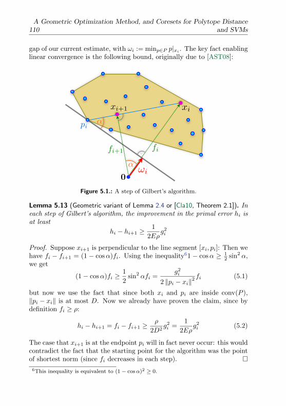
110A Geometric Optimization Method, and Coresets for Polytope Distance
and SVMs
gap of our current estimate, with ωi := minp∈P p|xi . The key fact enablinglinear convergence is the following bound, originally due to [AST08]:
xixi+1
i
pi
0
fifi+1
Figure 5.1.: A step of Gilbert’s algorithm.
Lemma 5.13 (Geometric variant of Lemma 2.4 or [Cla10, Theorem 2.1]). Ineach step of Gilbert’s algorithm, the improvement in the primal error hi isat least
hi − hi+1 ≥1
2Eρg2i
Proof. Suppose xi+1 is perpendicular to the line segment [xi, pi]: Then wehave fi − fi+1 = (1 − cosα)fi. Using the inequality61 − cosα ≥ 1
2 sin2 α,we get
(1− cosα)fi ≥1
2sin2 αfi =
g2i
2 ‖pi − xi‖2fi (5.1)
but now we use the fact that since both xi and pi are inside conv(P ),‖pi − xi‖ is at most D. Now we already have proven the claim, since bydefinition fi ≥ ρ:
hi − hi+1 = fi − fi+1 ≥ρ
2D2g2i =
1
2Eρg2i (5.2)
The case that xi+1 is at the endpoint pi will in fact never occur: this wouldcontradict the fact that the starting point for the algorithm was the pointof shortest norm (since fi decreases in each step).
6This inequality is equivalent to (1− cosα)2 ≥ 0.
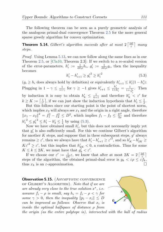
Upper Bounds: Algorithms to Construct Coresets 111
The following theorem can be seen as a purely geometric analysis ofthe analogous primal-dual convergence Theorem 2.5 for the more generalsparse greedy algorithm for convex optimization.
Theorem 5.14. Gilbert’s algorithm succeeds after at most 2⌈
2Eε
⌉many
steps.
Proof. Using Lemma 5.13, we can now follow along the same lines as in ourTheorem 2.5, or [Cla10, Theorem 2.3]: If we switch to a re-scaled versionof the error-parameters, h′i := 1
2Eρhi, g′i := 1
2Eρgi, then the inequalitybecomes
h′i − h′i+1 ≥ g′i2 ≥ h′i
2(5.3)
(gi ≥ hi does always hold by definition) or equivalently h′i+1 ≤ h′i(1− h′i):Plugging in 1 − γ ≤ 1
1+γ for γ ≥ −1 gives h′i+1 ≤ h′i1+h′i
= 11+ 1
h′i
. Then
by induction it is easy to obtain h′k ≤ 1k+1 and therefore h′k < ε′ for
k ≥ K :=⌈
1ε′⌉, if we can just show the induction hypothesis that h′1 ≤ 1
2 .But this follows since our starting point is the point of shortest norm,
which implies x2 will always see x1 and the origin in a right angle, therefore
‖x1 − x2‖2 = f21 − f2
2 ≤ D2, which implies f1 − f2 ≤ D2
2ρ and therefore
h′12 ≤ g′12 ≤ h′1 − h′2 ≤ 1
4 by using (5.3).Now we have obtained small h′i, but this does not necessarily imply yet
that g′i is also sufficiently small. For this we continue Gilbert’s algorithmfor another K steps, and suppose that in these subsequent steps, g′ alwaysremains ≥ ε′, then we always have that h′i−h′i+1 ≥ ε′2, and so h′K−h′2K ≥Kε′2 ≥ ε′, but this implies that h′2K < 0, a contradiction. Thus for someK ≤ k ≤ 2K, we must have that g′k < ε′.
If we choose our ε′ := 12E ε, we know that after at most 2K = 2
⌈2Eε
⌉steps of the algorithm, the obtained primal-dual error is gk < ερ ≤ εfk,thus xk is an ε-approximation.
0
s
x∗
Observation 5.15. (Asymptotic convergenceof Gilbert’s Algorithm). Note that if we areare already very close to the true solution x∗, i.e.assume fi − ρ is small, say hi = fi − ρ < γ forsome γ > 0, then the inequality ‖pi − xi‖ ≤ Dcan be improved as follows: Observe that xi isinside the optimal halfspace of distance ρ fromthe origin (as the entire polytope is), intersected with the ball of radius
112A Geometric Optimization Method, and Coresets for Polytope Distance
and SVMs
ρ+γ around the origin. Let s be the furthest distance from x∗ of any pointin this intersection area. It is easy to see that s = O(
√γ) is also small.
By triangle inequality we have ‖pi − xi‖ ≤ ‖pi − x∗‖+ s, so we get the
stronger inequality ‖pi − xi‖2 ≤ R2 +O(√γ) in the proof of Lemma 5.13.
Therefore, Gilbert’s algorithm always succeeds in at most
2⌈
2Eργ
⌉+ 2
⌈2(E∗+O(
√γ))
ε
⌉= 2
⌈2E∗(1+o(1))
ε
⌉many steps, as ε→ 0.
Note that the above analysis also proves the existence of ε-coresets of
size 2⌈
2Eε
⌉(and of size 2
⌈2E∗(1+o(1))
ε
⌉in the asymptotic notation), be-
cause the same improvement bound applies to the “exact” combinatorialalgorithm [Cla10, Algorithm 4.1] that, when adding a new point to theset, computes the exact polytope distance of the new set.
5.4.2. An Improved Version of Gilbert’s Algorithm forTwo Polytopes
Coresets for the distance between two polytopes. All coreset methodsfor the single polytope case can directly be applied to the distance prob-lem between two polytopes conv(P (1)) and conv(P (1)) by just running onthe Minkowski difference MD(P1, P2). This already makes the coreset ap-proach available for all machine learning methods corresponding to a twopolytope problem (as for example the standard SVM), see Section 5.5.
However, using the Minkowski difference has two major disadvantages:On one hand every vertex of MD(P1, P2) always corresponds to two originalvertices, one from each point class. Apart from potentially doubling thecoreset size, this is a very unfortunate restriction if the shapes of the twopoint classes are very unbalanced, as e.g. in the one-against-all approachfor multi-class classification, as it will create unnecessarily many non-zerocoefficients in the smaller class. On the other hand, to run Gilbert’s algo-rithm (or also the abstract version [Cla10, Algorithm 1.1] or the reducedhull variant [MST06]) on MD(P1, P2), we have to determine the startingpoint of shortest norm and therefore have to consider all pairs of originalpoints. Although this starting configuration was used in practice (see e.g.the DirectSVM [Roo00] and SimpleSVM [VSM03] implementations), thisshould definitely be avoided for large sets of points. We overcome bothdifficulties as follows:
An Improved Algorithm for Two Polytopes. The following modified al-
gorithm maintains a difference vector x(1)i −x
(2)i between the two polytopes,
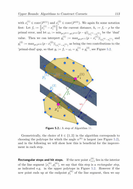
Upper Bounds: Algorithms to Construct Coresets 113
with x(1)i ∈ conv(P (1)) and x
(2)i ∈ conv(P (2)). We again fix some notation
first: Let fi :=∥∥∥x(1)
i − x(2)i
∥∥∥ be the current distance, hi := fi − ρ be the
primal error, and let ωi := minp∈P (1),q∈P (2)(p− q)|(x
(1)i −x
(2)i )
be the ’dual’
value. Then we can interpret g(1)i := maxp∈P (1)(p − x(1)
i )|(x
(2)i −x
(1)i )
and
g(2)i := maxp∈P (2)(p−x(2)
i )|(x
(1)i −x
(2)i )
as being the two contributions to the
’primal-dual’-gap, so that gi := fi − ωi = g(1)i + g
(2)i , see Figure 5.2.
x(1)i
x(2)i
g(2)i
g(1)i
p(1)i
p(2)i
fi
(1)
(2)
i
Figure 5.2.: A step of Algorithm 11.
Geometrically, the choice of k ∈ 1, 2 in the algorithm corresponds tochoosing the polytope for which the angle α(k) is largest (see Figure 5.2),and in the following we will show how this is beneficial for the improve-ment in each step.
Rectangular steps and hit steps. If the new point x(k)i+1 lies in the interior
of the line segment [x(k)i , p
(k)i ], we say that this step is a rectangular step,
as indicated e.g. in the upper polytope in Figure 5.2. However if the
new point ends up at the endpoint p(k)i of the line segment, then we say
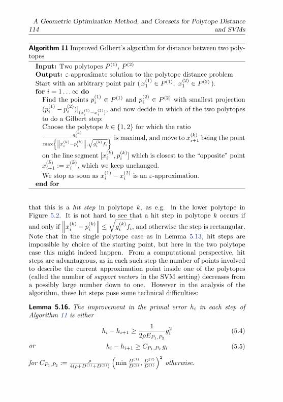
114A Geometric Optimization Method, and Coresets for Polytope Distance
and SVMs
Algorithm 11 Improved Gilbert’s algorithm for distance between two poly-topes
Input: Two polytopes P (1), P (2)
Output: ε-approximate solution to the polytope distance problem
Start with an arbitrary point pair (x(1)1 ∈ P (1), x
(2)1 ∈ P (2) ).
for i = 1 . . .∞ doFind the points p
(1)i ∈ P (1) and p
(2)i ∈ P (2) with smallest projection
(p(1)i − p
(2)i )|
(x(1)i −x
(2)i )
, and now decide in which of the two polytopes
to do a Gilbert step:Choose the polytope k ∈ 1, 2 for which the ratio
g(k)i
max
∥∥∥x(k)i −p
(k)i
∥∥∥,√g(k)i fi
is maximal, and move to x(k)i+1 being the point
on the line segment [x(k)i , p
(k)i ] which is closest to the “opposite” point
x(k)i+1 := x
(k)i , which we keep unchanged.
We stop as soon as x(1)i − x
(2)i is an ε-approximation.
end for
that this is a hit step in polytope k, as e.g. in the lower polytope inFigure 5.2. It is not hard to see that a hit step in polytope k occurs if
and only if∥∥∥x(k)
i − p(k)i
∥∥∥ ≤√g(k)i fi, and otherwise the step is rectangular.
Note that in the single polytope case as in Lemma 5.13, hit steps areimpossible by choice of the starting point, but here in the two polytopecase this might indeed happen. From a computational perspective, hitsteps are advantageous, as in each such step the number of points involvedto describe the current approximation point inside one of the polytopes(called the number of support vectors in the SVM setting) decreases froma possibly large number down to one. However in the analysis of thealgorithm, these hit steps pose some technical difficulties:
Lemma 5.16. The improvement in the primal error hi in each step ofAlgorithm 11 is either
hi − hi+1 ≥1
2ρEP1,P2
g2i (5.4)
or hi − hi+1 ≥ CP1,P2gi (5.5)
for CP1,P2:= ρ
4(ρ+D(1)+D(2))
(min D(1)
D(2) ,D(2)
D(1)
)2
otherwise.
Upper Bounds: Algorithms to Construct Coresets 115
Proof. Case R : In the case that the steps in both polytopes are rectan-gular we can follow the proof of Lemma 5.13: Assuming that the polytopechosen by the algorithm is k, we can follow (5.1) and (5.2) to get
hi − hi+1 ≥ ρ2
(g(k)i∥∥∥x(k)
i −p(k)i
∥∥∥)2
≥ ρ2
(maxm=1,2
g(m)i
D(m)
)2
≥ ρ2
(g(1)i +g
(2)i
D(1)+D(2)
)2
= 12ρEP1,P2
g2i , (5.6)
where we used max(ac ,
bd
)≥ a+b
c+d ∀a, b, c, d ≥ 0, Definition 5.6 of the Ex-
centricity, and that gi = g(1)i + g
(2)i .
Case M : In the “mixed” case that the step in one polytope (r) is rectan-
gular, but in the other polytope (h) is a hit step (due to∥∥∥x(h)
i − p(h)i
∥∥∥2
≤g
(h)i fi), we can argue as follows:
Case M(r) : If the algorithm chooses polytope (r), we can proceed
analogously to (5.6) to obtain
hi − hi+1 ≥ ρ2
g(r)i
2∥∥∥x(r)i −p
(r)i
∥∥∥2 = ρ2 max
g(r)i
2∥∥∥x(r)i −p
(r)i
∥∥∥2 , g(h)i
2
g(h)i fi
, (5.7)
but now there are two cases: If g(h)i fi ≤ D(h)2
, then we use the samearithmetic trick as in (5.6),
hi − hi+1 ≥ ρ2
(maxm=1,2
g(m)i
D(m)
)2
≥ 12ρEP1,P2
g2i . (5.8)
However if g(h)i fi ≥ D(h)2
, we have to argue differently: By the choice of
the algorithm we know that g(r)i ≥ g
(h)i because
g(r)i
fi=
g(r)i
2
g(r)i fi
≥ g(r)i
2∥∥∥x(r)i −p
(r)i
∥∥∥2 ≥g(h)i
fi. As in (5.7), the improvement in the step can then be bounded by
hi − hi+1 ≥ ρ2
g(r)i
2∥∥∥x(r)i −p
(r)i
∥∥∥2 ≥ ρ2
g(r)i
2
D(r)2≥ ρ
2
g(h)i g
(r)i
D(r)2which by our assumption
is ≥ ρ2D(h)2
D(r)2fig
(r)i ≥ ρ
2D(h)2
D(r)2fi
12
(g
(r)i + g
(h)i
)≥ CP1,P2gi . The last inequal-
ity follows because fi is always smaller than D(1) + D(2) + ρ by triangleinequality.
Case M(h) : If the choice criterium isg(r)i
2∥∥∥x(r)i −p
(r)i
∥∥∥2 ≤ g(h)i
2
g(h)i fi
, then
algorithm will choose the polytope (h) where a hit step will occur. The
116A Geometric Optimization Method, and Coresets for Polytope Distance
and SVMs
improvement in a hit step is worst if x(h)i+1 ends up exactly at distance√
fig(h)i from x
(h)i — i.e. on the Thales ball over fi — therefore f2
i −f2i+1 ≥
fig(h)i ⇒ hi − hi+1 = fi − fi+1 ≥ 1
2g(h)i ≥ ρ
2
g(h)i
fi. Now if we again assume
that g(h)i fi ≤ D(h)2
, then analogously to (5.7), (5.8) we have hi − hi+1≥ρ2
g(h)i
fi= ρ
2 max
g(r)i
2∥∥∥x(r)i −p
(r)i
∥∥∥2 , g(h)i
2
g(h)i fi
≥ 1
2ρEP1,P2g2i . On the other hand if
g(h)i fi ≥ D(h)2
, we distinguish two cases: First if g(h)i ≥ g(r)
i , then directly
hi−hi+1 ≥ 12g
(h)i ≥ 1
4 (g(h)i +g
(r)i ) = 1
4gi ≥ CP1,P2gi. Secondly if g(r)i ≥ g
(h)i ,
we use that by the choice of the algorithmg(h)i
fi≥ g
(r)i
2∥∥∥x(r)i −p
(r)i
∥∥∥2 ≥ g(r)i
2
D(r)2, so
we have hi − hi+1 ≥ ρ2
g(r)i
2
D(r)2≥ CP1,P2
gi analogous to the last part of the
previous case M(r).
Case H : If there is a hit step in both polytopes, then we use that the
algorithm has chosen the one with the larger value of g(k)i , therefore again
by the “angle constraint” reasoning that for hit steps f2i − f2
i+1 ≥ fig(k)i
we obtain fi − fi+1 ≥ fi2fig
(k)i = 1
2g(k)i ≥ 1
4gi ≥ CP1,P2gi.
Theorem 5.17. Algorithm 11 succeeds after at most
2⌈
2EP1,P2
ε
⌉+ 3 + 1
CP1,P2log D(1)+D(2)
ρCP1,P2ε = O(1/ε) many steps.
Proof. We count the steps of quadratic improvement (5.4) and those oflinear improvement (5.5) separately, using that each kind of step resultsin strict improvement in the primal error hi:
i) For quadratic improvement (5.4) we follow exactly along the proofof Theorem 5.14, for EP1,P2 being the pair excentricity: If we rescale byh′i := 1
2EP1,P2ρhi, (5.4) gives 1
h′i+1≥ 1 + 1
h′i. Now we just use that initially
h′1 is finite, therefore 1h′1≥ 0 and by induction we get 1
h′k≥ k − 1 for
all k ≥ 2. It follows that h′k ≤ ε′ for k ≥ K :=⌈
1ε′⌉
+ 1. By thesame argument as in the proof of Theorem 5.14, we have that after at
most 2K = 2⌈
2EP1,P2
ε
⌉+ 2 many rectangular steps, gk < ερ ≤ εfk, thus
x(1)k − x
(2)k is an ε-approximation.
ii) On the other hand we can bound the number of steps of linear im-provement (5.5) by an easier argument: Let C := CP1,P2 . Now hi−hi+1 ≥Cgi ≥ Chi is equivalent to hi+1 ≤ (1 − C)hi (recall that 0 < C < 1).Using that initially h1 ≤ D(1) + D(2), we get hk ≤ (1 − C)k−1h1 ≤
Upper Bounds: Algorithms to Construct Coresets 117
(1 − C)k−1(D(1) + D(2)) for all k ≥ 2, which is ≤ ε′ as soon as k − 1 ≥log D(1)+D(2)
ε′− log(1−C) , which in particular holds if k − 1 ≥ 1
C log D(1)+D(2)
ε′ by using
the inequality λ < − log(1 − λ) for 0 < λ < 1. For ε′ := ρC ε, this isenough because ε′ ≥ hk ≥ hk − hk+1 ≥ Cgk implies gk ≤ ερ ≤ εfk, orin other words the algorithm obtains an ε-approximation after at most1C log D(1)+D(2)
ρC ε + 1 many steps of linear improvement.
Generalization of our algorithm for convex optimization over products ofsimplices. We can also generalize our above new variant of sparse greedyapproximation in terms of the general framework by Clarkson [Cla10],when we extend it to solving any concave maximization problem over aproduct of finitely many simplices or convex hulls. To do so, we can provethe same step improvement (5.4) also for the case of convex functionsdefined on any product of simplices. We are currently investigating thedetails in this setting.
5.4.3. Smaller Coresets by “Away” Steps
Gilbert’s algorithm and also its “exact” variant, due to their greedy nature,are not optimal in the size of the coresets they deliver. However, Clarksonshowed that a modified procedure [Cla10, Algorithm 5.1] based on an ideaby [TY07], called the away steps algorithm, obtains smaller coresets. Thefollowing Theorem, together with our lower bounds from Section 5.3.1,will settle the question on the size of coresets for the distance problem ofone polytope to the origin, because the size of the coreset obtained by thealgorithm matches our lower bound, and therefore is best possible:
Theorem 5.18. For any ε > 0, the away steps algorithm [Cla10, Algorithm
5.1] returns an ε-coreset of size at most⌈Eε
⌉, and at most
⌈E∗(1+o(1))
ε
⌉as
ε→ 0.
Proof. We consider the equivalent convex optimization description of thepolytope distance problem by f(x) = ‖Ax‖, as described in our Sec-tion 5.2.3. In this setting, [Cla10, Theorem 5.1] shows that the awaysteps algorithm delivers a subset of coordinate indices N of size
⌈1ε′⌉
suchthat f(xN )−ω(xN ) ≤ 2Cfε
′, where xN is the true optimal solution of theproblem restricted to the coordinates in N . By the scaling ε′ := ρε
2Cf, this
means that in our setting, the away steps algorithm returns an ε-coreset
of size⌈
2Cfρε
⌉≤⌈Eε
⌉, and
⌈2C∗f (1+o(1)
ρε
⌉≤⌈E∗(1+o(1)
ε
⌉in the asymptotic
case; the last two inequalities holding by Lemma 5.7.
118A Geometric Optimization Method, and Coresets for Polytope Distance
and SVMs
Away steps in the case of two polytopes. We can adjust [Cla10, Algo-rithm 5.1] for two polytopes as follows: Start with the closest point pair
(x(1)1 ∈ P (1), x
(2)1 ∈ P (2) ), and proceed as in [Cla10, Algorithm 5.1]. In
each step choose the polytope according to the choice criterium of our Al-gorithm 11, but with the modification that whenever a hit step is possibleone either side, we choose to do this hit step.
Theorem 5.19. For any ε > 0, the modified away steps algorithm on
two polytopes returns an ε-coreset of size at most⌈EP1,P2
ε
⌉, and at most⌈
E∗P1,P2(1+o(1))
ε
⌉as ε→ 0.
Proof. Sketch: We can follow the proof of [Cla10, Theorem 5.1] usingour Lemma 5.16, and observe that a hit step never increases the coresetsize. The key point is that for any step that increases the coreset size,the improvement bound (5.4) always holds. The induction hypothesish′1 := 1
2EP1,P2ρh1 ≤ 1
2 follows if we start at the closest pair.
5.5. Applications to Machine Learning
The advantage of the coreset approach is that both the running time ofthe algorithms and the sparsity of the obtained solutions is independentof the dimension d of the space and independent of the number of pointsn. This property makes the approach very attractive for kernel methods,where the points are implicitly assumed to live in a (possibly very highdimensional) feature space.
Table 5.5 briefly recapitulates the fact that nearly all well known SVMvariants are equivalent to a polytope distance problem between either oneor two polytopes, showing that all these variants do fit into our frame-work of coresets. This also holds for the soft-margin variants [CV95] if thepunishment of the outliers is proportional to the squared distance to theclassification hyperplane (`2-loss SVM). In the table, xi ∈ Rd, 1 ≤ i ≤ ndenote the original points, φ(xi) are their implicit images in the featurespace defined by the kernel, and in the two class cases the labels of thepoints are given by yi = ±1. ω and b are the normal and offset of the max-imum margin hyperplane that we are searching for, and the ξi representslack variables for the case of possible (punished) outliers.
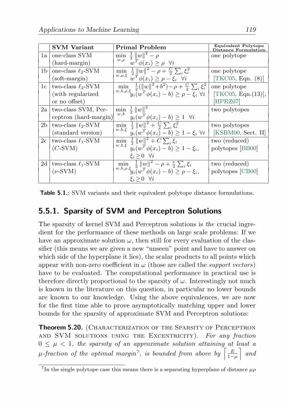
Applications to Machine Learning 119
SVM Variant Primal Problem Equivalent PolytopeDistance Formulation
1a one-class SVM minw,ρ
12‖w‖2 − ρ one polytope
(hard-margin) wTφ(xi) ≥ ρ ∀i1b one-class `2-SVM min
w,ρ,ξ
12‖w‖2 − ρ+ C
2
∑i ξ
2i one polytope
(soft-margin) wTφ(xi) ≥ ρ− ξi ∀i [TKC05, Eqn. (8)]
1c two-class `2-SVM minw,b,ρ,ξ
12(‖w‖2+b2)−ρ+ C
2
∑i ξ
2i one polytope
(with regularized yi(wTφ(xi)− b) ≥ ρ− ξi ∀i [TKC05, Eqn.(13)],
or no offset) [HPRZ07]
2a two-class SVM, Per- minw,b
12‖w‖2 two polytopes
ceptron (hard-margin) yi(wTφ(xi)− b) ≥ 1 ∀i
2b two-class `2-SVM minw,b,ξ
12‖w‖2 + C
2
∑i ξ
2i two polytopes
(standard version) yi(wTφ(xi)− b) ≥ 1− ξi ∀i [KSBM00, Sect. II]
2c two-class `1-SVM minw,b,ξ
12‖w‖2 + C
∑i ξi two (reduced)
(C-SVM) yi(wTφ(xi)− b) ≥ 1− ξi, polytopes [BB00]
ξi≥0 ∀i2d two-class `1-SVM min
w,b,ρ,ξ
12‖w‖2 − ρ+ ν
2
∑i ξi two (reduced)
(ν-SVM) yi(wTφ(xi)− b) ≥ ρ− ξi, polytopes [CB00]
ξi≥0 ∀i
Table 5.1.: SVM variants and their equivalent polytope distance formulations.
5.5.1. Sparsity of SVM and Perceptron Solutions
The sparsity of kernel SVM and Perceptron solutions is the crucial ingre-dient for the performance of these methods on large scale problems: If wehave an approximate solution ω, then still for every evaluation of the clas-sifier (this means we are given a new “unseen” point and have to answer onwhich side of the hyperplane it lies), the scalar products to all points whichappear with non-zero coefficient in ω (those are called the support vectors)have to be evaluated. The computational performance in practical use istherefore directly proportional to the sparsity of ω. Interestingly not muchis known in the literature on this question, in particular no lower boundsare known to our knowledge. Using the above equivalences, we are nowfor the first time able to prove asymptotically matching upper and lowerbounds for the sparsity of approximate SVM and Perceptron solutions:
Theorem 5.20. (Characterization of the Sparsity of Perceptronand SVM solutions using the Excentricity). For any fraction0 ≤ µ < 1, the sparsity of an approximate solution attaining at least a
µ-fraction of the optimal margin7, is bounded from above by⌈
E1−µ
⌉and
7In the single polytope case this means there is a separating hyperplane of distance µρ
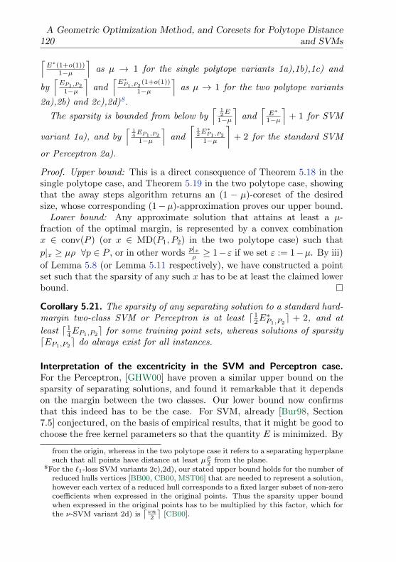
120A Geometric Optimization Method, and Coresets for Polytope Distance
and SVMs⌈E∗(1+o(1))
1−µ
⌉as µ → 1 for the single polytope variants 1a),1b),1c) and
by⌈EP1,P2
1−µ
⌉and
⌈E∗P1,P2
(1+o(1))
1−µ
⌉as µ → 1 for the two polytope variants
2a),2b) and 2c),2d)8.
The sparsity is bounded from below by⌈
12E
1−µ
⌉and
⌈E∗
1−µ
⌉+ 1 for SVM
variant 1a), and by⌈
14EP1,P2
1−µ
⌉and
⌈12E∗P1,P2
1−µ
⌉+ 2 for the standard SVM
or Perceptron 2a).
Proof. Upper bound: This is a direct consequence of Theorem 5.18 in thesingle polytope case, and Theorem 5.19 in the two polytope case, showingthat the away steps algorithm returns an (1 − µ)-coreset of the desiredsize, whose corresponding (1−µ)-approximation proves our upper bound.
Lower bound: Any approximate solution that attains at least a µ-fraction of the optimal margin, is represented by a convex combinationx ∈ conv(P ) (or x ∈ MD(P1, P2) in the two polytope case) such that
p|x ≥ µρ ∀p ∈ P , or in other words p|xρ ≥ 1−ε if we set ε := 1−µ. By iii)
of Lemma 5.8 (or Lemma 5.11 respectively), we have constructed a pointset such that the sparsity of any such x has to be at least the claimed lowerbound.
Corollary 5.21. The sparsity of any separating solution to a standard hard-margin two-class SVM or Perceptron is at least d 1
2E∗P1,P2
e + 2, and at
least d 14EP1,P2
e for some training point sets, whereas solutions of sparsitydEP1,P2
e do always exist for all instances.
Interpretation of the excentricity in the SVM and Perceptron case.For the Perceptron, [GHW00] have proven a similar upper bound on thesparsity of separating solutions, and found it remarkable that it dependson the margin between the two classes. Our lower bound now confirmsthat this indeed has to be the case. For SVM, already [Bur98, Section7.5] conjectured, on the basis of empirical results, that it might be good tochoose the free kernel parameters so that the quantity E is minimized. By
from the origin, whereas in the two polytope case it refers to a separating hyperplanesuch that all points have distance at least µ ρ
2from the plane.
8For the `1-loss SVM variants 2c),2d), our stated upper bound holds for the number ofreduced hulls vertices [BB00, CB00, MST06] that are needed to represent a solution,however each vertex of a reduced hull corresponds to a fixed larger subset of non-zerocoefficients when expressed in the original points. Thus the sparsity upper boundwhen expressed in the original points has to be multiplied by this factor, which forthe ν-SVM variant 2d) is
⌈νn2
⌉[CB00].
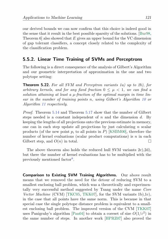
Applications to Machine Learning 121
our derived bounds we can now confirm that this choice is indeed good inthe sense that it result in the best possible sparsity of the solutions. [Bur98,Theorem 6] also showed that E gives an upper bound for the VC dimensionof gap tolerant classifiers, a concept closely related to the complexity ofthe classification problem.
5.5.2. Linear Time Training of SVMs and Perceptrons
The following is a direct consequence of the analysis of Gilbert’s Algorithmand our geometric interpretation of approximation in the one and twopolytope setting:
Theorem 5.22. For all SVM and Perceptron variants 1a) up to 2b), forarbitrary kernels, and for any fixed fraction 0 ≤ µ < 1, we can find asolution attaining at least a µ-fraction of the optimal margin in time lin-ear in the number of training points n, using Gilbert’s Algorithm 10 orAlgorithm 11 respectively.
Proof. Theorem 5.14 and Theorem 5.17 show that the number of Gilbertsteps needed is a constant independent of n and the dimension d. Bykeeping the lengths of all projections onto the previous estimate in memory,one can in each step update all projections by just calculating n scalarproducts (of the new point pi to all points in P ) [KSBM00], therefore thenumber of kernel evaluations (scalar product computations) is n in eachGilbert step, and O(n) in total.
The above theorem also holds the reduced hull SVM variants 2c),2d),but there the number of kernel evaluations has to be multiplied with thepreviously mentioned factor8.
Comparison to Existing SVM Training Algorithms. Our above resultmeans that we removed the need for the detour of reducing SVM to asmallest enclosing ball problem, which was a theoretically and experimen-tally very successful method suggested by Tsang under the name CoreVector Machine (CVM) [TKC05, TKK07], for the SVM variants 1b),1c),in the case that all points have the same norm. This is because in thatspecial case the single polytope distance problem is equivalent to a small-est enclosing ball problem. The improved version of the CVM [TKK07]uses Panigrahy’s algorithm [Pan04] to obtain a coreset of size O(1/ε2) inthe same number of steps. In another work [HPRZ07] also proved the
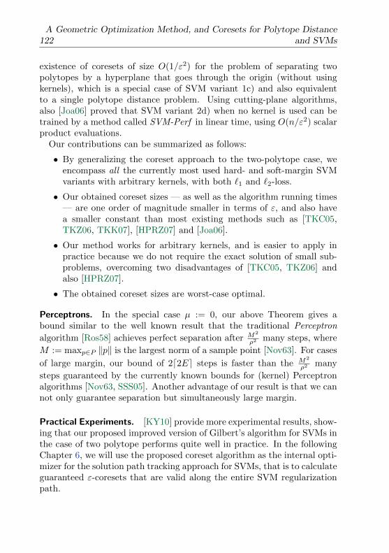
122A Geometric Optimization Method, and Coresets for Polytope Distance
and SVMs
existence of coresets of size O(1/ε2) for the problem of separating twopolytopes by a hyperplane that goes through the origin (without usingkernels), which is a special case of SVM variant 1c) and also equivalentto a single polytope distance problem. Using cutting-plane algorithms,also [Joa06] proved that SVM variant 2d) when no kernel is used can betrained by a method called SVM-Perf in linear time, using O(n/ε2) scalarproduct evaluations.
Our contributions can be summarized as follows:
• By generalizing the coreset approach to the two-polytope case, weencompass all the currently most used hard- and soft-margin SVMvariants with arbitrary kernels, with both `1 and `2-loss.
• Our obtained coreset sizes — as well as the algorithm running times— are one order of magnitude smaller in terms of ε, and also havea smaller constant than most existing methods such as [TKC05,TKZ06, TKK07], [HPRZ07] and [Joa06].
• Our method works for arbitrary kernels, and is easier to apply inpractice because we do not require the exact solution of small sub-problems, overcoming two disadvantages of [TKC05, TKZ06] andalso [HPRZ07].
• The obtained coreset sizes are worst-case optimal.
Perceptrons. In the special case µ := 0, our above Theorem gives abound similar to the well known result that the traditional Perceptron
algorithm [Ros58] achieves perfect separation after M2
ρ2 many steps, where
M := maxp∈P ‖p‖ is the largest norm of a sample point [Nov63]. For cases
of large margin, our bound of 2d2Ee steps is faster than the M2
ρ2 many
steps guaranteed by the currently known bounds for (kernel) Perceptronalgorithms [Nov63, SSS05]. Another advantage of our result is that we cannot only guarantee separation but simultaneously large margin.
Practical Experiments. [KY10] provide more experimental results, show-ing that our proposed improved version of Gilbert’s algorithm for SVMs inthe case of two polytope performs quite well in practice. In the followingChapter 6, we will use the proposed coreset algorithm as the internal opti-mizer for the solution path tracking approach for SVMs, that is to calculateguaranteed ε-coresets that are valid along the entire SVM regularizationpath.
6Solution Paths for Convex
Optimization Problems overVectors
We consider parameterized convex optimization problems over the unitsimplex or over the box, that depend on a single additional parameter.We provide a simple and efficient scheme for maintaining an ε-approximatesolution (and a corresponding ε-coreset) along the entire parameter path.We prove correctness and optimality of the method. Practically relevantinstances of our studied parameterized optimization problems include forexample regularization paths of support vector machines (SVMs), multi-ple kernel learning, `1-regularized least squares or logistic regression, orgeometric problems such as the minimum enclosing ball of moving points.
This is joint work with Joachim Giesen and Soeren Laue [GJL10, GJL12a].
6.1. Introduction
We study convex optimization problems that are parameterized by a singleparameter. We are interested in the whole solution path in that parameter,
123
124 Solution Paths for Convex Optimization Problems over Vectors
i.e. the set of optimal solutions for all parameter values. We provide a sim-ple algorithmic framework for tracking guaranteed approximate solutionsalong the parameter path. We obtain strict guarantees on the approxi-mation quality (continuously along the path) as well as the running time.The main idea of our scheme is to compute at a parameter value an ap-proximate solution that is slightly better than the required quality, andthen to keep this solution as the parameter changes, exactly as long as therequired approximation quality can still be guaranteed. Only when theapproximation quality is no longer sufficient, a new solution is computed.
We prove that, if an approximation guarantee of ε > 0 is required forthe entire path, then the number of necessary updates along the path isonly O
(1ε
), independently of the number of variables used. We also show
that this obtained path complexity of O(
1ε
)is indeed best possible.
The practical need to understand the entire path of (near) optimal solu-tions to parameterized problems comes from many different fields, such ascontrol theory, various multi-objective optimization applications, and mostnotably from regularization methods in machine learning. The question ofparameter selection — e.g. the choice of the best regularization parameter— is often a non-trivial task. Many approaches have been proposed in thelast decade for tracking exact solution paths for optimization problems,in the case that the paths are piecewise linear. However there are manyapplications where this assumption does not hold, and even if it does, thepath might have exponential complexity in the worst case [GJM10]. Ournew framework strongly contrasts the existing approaches in the litera-ture, and proves a path complexity independent of the input size (onlydepending on the desired approximation accuracy ε), for a wider class ofproblems.
Our framework is not tied to a specific algorithm, and very simple to im-plement: Any existing optimizer or heuristic of choice can be used to com-pute an approximate solution at fixed parameter values. Warm-startingthe optimizer with the previous solution at each update step can be usedto further improve speed in practice.
Parameterized Optimization. Our goal is to compute the entire solutionpath (with a continuously guaranteed approximation quality) for parame-terized optimization problems over the ‖.‖1-ball, the ‖.‖∞-ball, or the unitsimplex., i.e. optimization problems of the form (3.3)
minx∈Rn
ft(x)
s.t. ‖x‖1 ≤ 1 ,(6.1)
Introduction 125
or the analogous box-constrained variant (3.4)
minx∈Rn
ft(x)
s.t. ‖x‖∞ ≤ 1 ,(6.2)
or problems over the simplex as in (3.1), i.e.,
minx∈Rn
ft(x)
s.t. ‖x‖1 = 1 ,x ≥ 0 ,
(6.3)
where ft is a family of convex functions, parameterized by t ∈ R. Note thata variety of other problems can also be reduced to the above form (6.1), (6.2)or (6.3), by introducing “slack” variables and/or re-scaling. All three for-mulations have prominent applications in various areas.
Motivation and Applications. Despite our path framework being verysimple, we demonstrate that it is well applicable for practical large scaleproblems. Our experiments demonstrate that the computation of an entireε-approximate solution path is only marginally more expensive than thecomputation of a single approximate solution.
Our work is motivated by several important machine learning tech-niques, some of which we have mentioned in Chapters 2 and 3, whichnaturally come with a parameter that is non-trivial to choose (e.g. a regu-larization parameter). We apply the algorithm to compute the entire regu-larization path for `1-regularized least squares (also known as basis pursuitde-noising in compressed sensing [CDS98, FNW07]), the Lasso [Tib96], `1-regularized logistic regression [KKB07], support vector machines (SVMs),and to find the best combination of two kernels, which is a special case ofmultiple kernel learning [BLJ04].
Other applications that directly fit into our framework include `2-supportvector regression (SVR), AdaBoost, mean-variance analysis in portfolio se-lection [Mar52], the smallest enclosing ball problem [BC07], and also anybox-constrained convex optimization problems.
Related Work. Solution path algorithms (sometimes also called homo-topy methods) have a long history, in particular in the optimization com-munity [Rit62, Rit84, Osb92] and in control theory (e.g. model predic-tive control, [GPM89, HHB99]). More recently these methods had anindependent revival in machine learning, in particular for computing ex-act solution paths in the context of support vector machines and related
126 Solution Paths for Convex Optimization Problems over Vectors
problems [HRTZ04, WZLS08, GGJW09], and also regression techniquessuch as `1-regularized least squares [OPT00, EHJT04, MCW05, Tur05,RZ07, HYZ08]. Similar methods were also applied by [EHJT04, GZ05,LC06, WCYL06, BHH06, WYL06, LGC07, LS07, Wan08] to special casesof quadratic programs, in particular cases where the solution path is piece-wise linear. However, three relatively severe problems remained unresolvedto large parts:
i) The assumption of piecewise linearity of the path does only holdfor a small class of parameterized optimization problems, mostlyquadratic programs with linearly parameterized objective or righthand side [GGJW09].
ii) The complexity of exact solution paths can be very large in the worstcase, e.g., it can grow exponentially in the input size as it has beenshown for support vector machines with `1-loss [GJM10].
iii) Almost all of the above mentioned existing path algorithms rely onthe inversion of principal sub-matrices of large matrices, leading tonumerical instability as well as combinatorial problems [HRTZ04,Section 5.2], [GGJW09].
Our proposed framework here overcomes the above issues by movingaway from exact solution paths, towards paths of guaranteed ε-approx-imation quality. Our algorithm works for arbitrary non-linear solutionpaths, under weak continuity assumptions.
Approximation algorithms and warm-start heuristics for parameter se-lection have gained interest in various areas, such as e.g. in machine learn-ing [FHHT07, KKB07], compressed sensing [HYZ08], or multi-objectiveoptimization [BGP09]. However, to the best of our knowledge, so far noapproximation guarantees along the path could be given for these existingalgorithms, which sample the path at discrete parameter values.
6.2. Approximation Quality Measures
In this small section we will briefly recall the practical approximation qual-ity measures for convex optimization problems of the form (6.3) and (6.2),which we have proposed in Chapter 2 using the “poor-man’s” duality ap-proach. For this it will be crucial to consider the gradient ∇ft(x) of theobjective function ft with respect to x. We assume the function ft(x) tobe convex and continuously differentiable in x, for each t ∈ R.
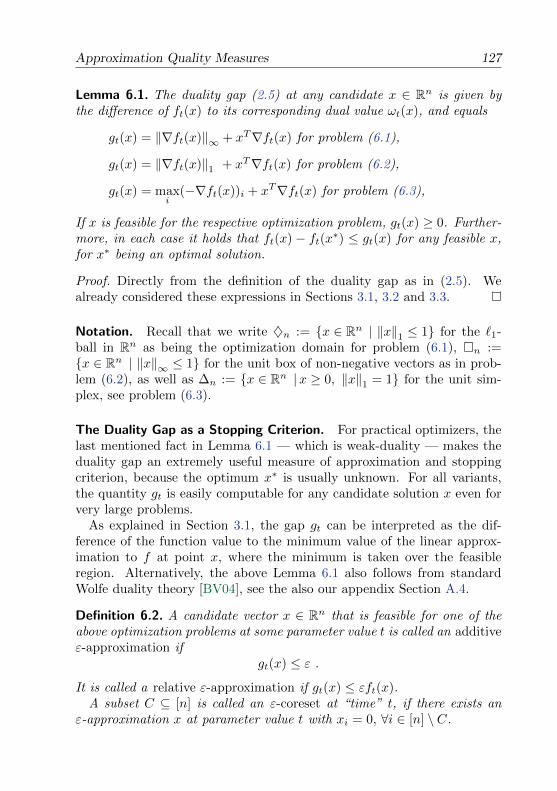
Approximation Quality Measures 127
Lemma 6.1. The duality gap (2.5) at any candidate x ∈ Rn is given bythe difference of ft(x) to its corresponding dual value ωt(x), and equals
gt(x) = ‖∇ft(x)‖∞ + xT∇ft(x) for problem (6.1),
gt(x) = ‖∇ft(x)‖1 + xT∇ft(x) for problem (6.2),
gt(x) = maxi
(−∇ft(x))i + xT∇ft(x) for problem (6.3),
If x is feasible for the respective optimization problem, gt(x) ≥ 0. Further-more, in each case it holds that ft(x) − ft(x∗) ≤ gt(x) for any feasible x,for x∗ being an optimal solution.
Proof. Directly from the definition of the duality gap as in (2.5). Wealready considered these expressions in Sections 3.1, 3.2 and 3.3.
Notation. Recall that we write ♦n := x ∈ Rn | ‖x‖1 ≤ 1 for the `1-ball in Rn as being the optimization domain for problem (6.1), n :=x ∈ Rn | ‖x‖∞ ≤ 1 for the unit box of non-negative vectors as in prob-lem (6.2), as well as ∆n := x ∈ Rn |x ≥ 0, ‖x‖1 = 1 for the unit sim-plex, see problem (6.3).
The Duality Gap as a Stopping Criterion. For practical optimizers, thelast mentioned fact in Lemma 6.1 — which is weak-duality — makes theduality gap an extremely useful measure of approximation and stoppingcriterion, because the optimum x∗ is usually unknown. For all variants,the quantity gt is easily computable for any candidate solution x even forvery large problems.
As explained in Section 3.1, the gap gt can be interpreted as the dif-ference of the function value to the minimum value of the linear approx-imation to f at point x, where the minimum is taken over the feasibleregion. Alternatively, the above Lemma 6.1 also follows from standardWolfe duality theory [BV04], see the also our appendix Section A.4.
Definition 6.2. A candidate vector x ∈ Rn that is feasible for one of theabove optimization problems at some parameter value t is called an additiveε-approximation if
gt(x) ≤ ε .It is called a relative ε-approximation if gt(x) ≤ εft(x).
A subset C ⊆ [n] is called an ε-coreset at “time” t, if there exists anε-approximation x at parameter value t with xi = 0, ∀i ∈ [n] \ C.
128 Solution Paths for Convex Optimization Problems over Vectors
Relative Approximation. When considering relative approximation, weassume that ft(x) ≥ 0 for all x in the domain. Sometimes in the literature,a multiplicative ε-approximation is defined more restrictively as g(x) ≤εf(x∗), relative to the optimal value f(x∗) of the primal optimizationproblem. Note that this can directly be obtained from our slightly weakerdefinition by setting ε in the definition of an ε-approximation to ε′ := ε
1+ε ,because g(x) ≤ ε
1+εf(x)⇔ (1+ε)(f(x)−ω(x)) ≤ εf(x)⇔ g(x) ≤ εω(x) ≤εf(x∗), recalling weak duality from Section 2.2. Note that when lookingat the relative error for maximization instead of minimization problems,no such distinction is necessary.
6.3. Optimizing Parameterized Functions
We are interested in ε-approximations for problems (6.1), (6.2) and (6.3)for all valid parameter values t ∈ R, and will study the complexity of suchsolution paths in the following.
Definition 6.3. The ε-approximation path complexity of a parameterizedoptimization problem is defined as the minimum number of intervals overall possible partitions of the parameter range [tmin, tmax] ⊆ R, such that foreach individual interval, there is a single solution that is an ε-approximationfor that entire interval.
The following simple lemma is at the core of our discussion and char-acterizes how far we can change the parameter t such that a given ε
γ -
approximate solution x (for γ > 1) at t stays an ε-approximate solution.The idea is a simple continuity argument for the duality gap, as the pa-rameter changes. Lemma 6.4 gives the stability result for the case ofbounded `1-norm (6.1), and Lemma 6.5 considers the `∞-case (6.2), whichis in a sense dual to the `1-case. The lemmata each give two alternativeconditions, which both imply the desired stability of the approximation.Two important consequences will follow from these stability results: Firstwe will obtain that the global ε-approximation path complexity is O( 1
ε ).Secondly, for most practical problems, we will be able to locally exactlycompute the largest possible parameter-interval over which some specificε-approximate solution stays valid, which in practice will lead to intervalsmuch longer than the worst-case upper bound.
Optimizing Parameterized Functions 129
6.3.1. Stability of ε-Approximations
Lemma 6.4 (Stability of an Approximation under Bounded `1-Norm). Letx ∈ ♦n be an ε
γ -approximation to problem (6.1) for some fixed parameter
value t, for some γ > 1. Then for all t′ ∈ R that satisfy either
gt′(x)− gt(x) =‖∇ft′(x)‖∞ − ‖∇ft(x)‖∞+xT
(∇ft′(x)−∇ft(x)
) ≤ ε(
1− 1
γ
), (6.4)
or
(1 + ‖x‖1) ‖∇ft′(x)−∇ft(x)‖∞ ≤ ε(
1− 1
γ
), (6.5)
it holds that the solution x is still an ε-approximation to problem (6.1) atthe changed parameter value t′.
Proof. We first prove the statement assuming that (6.4) is satisfied. Todo so, we add to (6.4) the inequality stating that x is an ε
γ -approximatesolution at value t, i.e.
‖∇ft(x)‖∞ + xT∇ft(x) ≤ ε
γ.
This directly results in the claimed bound ‖∇ft′(x)‖∞ + xT∇ft′(x) ≤ εon the duality gap at t′.
We will prove the second part of the lemma by showing that the secondcondition (6.5) in fact implies the condition (6.4). On one hand, by the(reversed) triangle inequality, the first term in (6.4) is upper bounded asfollows.
‖∇ft′(x)‖∞ − ‖∇ft(x)‖∞ ≤ ‖∇ft′(x)−∇ft(x)‖∞ .
On the other hand, from the general norm inequality1 xT y ≤ ‖x‖ · ‖y‖∗together with the fact that the `∞-norm is dual to the `1-norm, we have
xT (∇ft′(x)−∇ft(x)) ≤ ‖x‖1 · ‖∇ft′(x)−∇ft(x)‖∞ .
Altogether, this means that (6.5) implies (6.4), or in other words we havereduced the case to the already verified first case of the lemma.
1The inequality xT y ≤ ‖x‖ · ‖y‖∗ can be seen as the generalization of the Cauchy-Schwarz inequality to arbitrary norms ‖.‖ and their corresponding dual norms‖y‖∗ := sup
‖x‖≤1xT y, and follows directly from the definition of the dual norm.
130 Solution Paths for Convex Optimization Problems over Vectors
Lemma 6.5 (Stability of an Approximation under Bounded `∞-Norm). Letx ∈ n be an ε
γ -approximation to problem (6.2) for some fixed parameter
value t, for some γ > 1. Then for all t′ ∈ R that satisfy either
gt′(x)− gt(x) =‖∇ft′(x)‖1 − ‖∇ft(x)‖1+xT
(∇ft′(x)−∇ft(x)
) ≤ ε(
1− 1
γ
), (6.6)
or
(1 + ‖x‖∞) ‖∇ft′(x)−∇ft(x)‖1 ≤ ε(
1− 1
γ
), (6.7)
it holds that the solution x is still an ε-approximation to problem (6.2) atthe changed parameter value t′.
Proof. Completely analogous to the proof of Lemma 6.4, by swapping theroles of ‖.‖1 and ‖.‖∞.
Lemma 6.6 (Stability of an Approximation over the Simplex). Let x ∈ ∆n
be an εγ -approximation to problem (6.3) for some fixed parameter value t,
for some γ > 1. Then for all t′ ∈ R that satisfy either
gt′(x)− gt(x) =maxi
(∇ft(x)−∇ft′(x)
)i
+xT(∇ft′(x)−∇ft(x)
) ≤ ε
(1− 1
γ
), (6.8)
or
(1 + ‖x‖1) ‖∇ft′(x)−∇ft(x)‖∞ ≤ ε(
1− 1
γ
), (6.9)
it holds that the solution x is still an ε-approximation to problem (6.3) atthe changed parameter value t′.
Proof. Using the inclusion ∆n ⊂ ♦n, we can follow the same proof as inLemma 6.4. Then the first claim will follow from the fact that
maxi
(∇ft(x)−∇ft′(x)
)i≤ ‖∇ft′(x)−∇ft(x)‖∞ ,
see also the definition of the duality gap given in Lemma 6.1 for the simplexdomain.
6.3.2. Bounding the Path Complexity
The following main theorem on the path complexity bounds the param-eter interval lengths in the worst case. Here we assume that the globalparameter range of interest, [tmin, tmax] ⊂ R, is finite.
Optimizing Parameterized Functions 131
Theorem 6.7. Let ft be convex and continuously differentiable in x, andlet ∇ft(x) be Lipschitz continuous in t for all feasible x. Then the ε-approximation path complexity of problems (6.1), (6.2) and (6.3) over theparameter range t ∈ [tmin, tmax] ⊂ R is O
(1ε
).
Proof. We prove the `1-case first. In order for the condition (6.5) inLemma 6.4 to be satisfied, we first use that for any x ∈ ♦n,
(1 + ‖x‖1) ‖∇ft′(x)−∇ft(x)‖∞≤ 2 · ‖∇ft′(x)−∇ft(x)‖∞≤ 2 · L · |t′ − t| .
Here L is the supremum of the Lipschitz constants with respect to t of thederivatives ∇ft(x), taken over the compact feasible domain ♦n for x. Itfollows that condition (6.5) in the Lemma is satisfied for any x ∈ ♦n, ifwe require the parameter intervals to be of length |t′ − t| ≤ ε
2L
(1− 1
γ
).
Dividing the total parameter range |tmax − tmin| by this interval length,the claim follows directly: The path complexity is at most⌈
1ε · |tmax − tmin| · 2L γ
γ−1
⌉.
For the `∞-case, we argue the same way, applying condition (6.7). Thecase of optimization over the simplex also follows from the argument forthe `1-case.
Optimality. One might expect that the above path complexity result ofO(
1ε
)is best possible. As ∇ft(x) changes with t, the interval length where
gt(x) ≤ ε holds can not be larger than Θ(ε) in the worst case. The nextsmall section will formally prove that the path complexity obtained aboveis indeed worst-case optimal.
6.3.3. Lower Bound
We provide an explicit lower bound on the path complexity for optimizingover the simplex (being a subset of the `1-ball ♦n), showing that the abovecomplexity from Theorem 6.7 is indeed best possible up to a constantfactor. We consider the following instance of a parameterized optimizationproblem (6.3) or (6.1):
minimizex∈Rn
ft(x) := xTh(t)
s.t. x ∈ ∆n
(6.10)
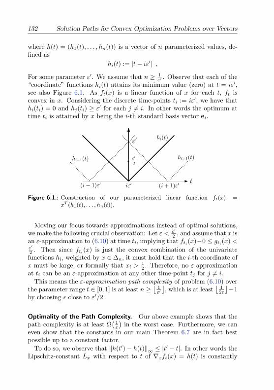
132 Solution Paths for Convex Optimization Problems over Vectors
where h(t) = (h1(t), . . . , hn(t)) is a vector of n parameterized values, de-fined as
hi(t) := |t− iε′| ,
For some parameter ε′. We assume that n ≥ 1ε′ . Observe that each of the
“coordinate” functions hi(t) attains its minimum value (zero) at t = iε′,see also Figure 6.1. As ft(x) is a linear function of x for each t, ft isconvex in x. Considering the discrete time-points ti := iε′, we have thathi(ti) = 0 and hj(ti) ≥ ε′ for each j 6= i. In other words the optimum attime ti is attained by x being the i-th standard basis vector ei.
iε′(i− 1)ε′ (i+ 1)ε′t
hi(t)
hi+1(t)hi−1(t)
ε′
ε′2
Figure 6.1.: Construction of our parameterized linear function ft(x) =xT (h1(t), . . . , hn(t)).
Moving our focus towards approximations instead of optimal solutions,we make the following crucial observation: Let ε < ε′
2 , and assume that x isan ε-approximation to (6.10) at time ti, implying that fti(x)−0 ≤ gti(x) <ε′
2 . Then since fti(x) is just the convex combination of the univariatefunctions hi, weighted by x ∈ ∆n, it must hold that the i-th coordinate ofx must be large, or formally that xi >
12 . Therefore, no ε-approximation
at ti can be an ε-approximation at any other time-point tj for j 6= i.
This means the ε-approximation path complexity of problem (6.10) overthe parameter range t ∈ [0, 1] is at least n ≥
⌊1ε′⌋, which is at least
⌊12ε
⌋−1
by choosing ε close to ε′/2.
Optimality of the Path Complexity. Our above example shows that thepath complexity is at least Ω
(1ε
)in the worst case. Furthermore, we can
even show that the constants in our main Theorem 6.7 are in fact bestpossible up to a constant factor.
To do so, we observe that ‖h(t′)− h(t)‖∞ ≤ |t′ − t|. In other words theLipschitz-constant Lx with respect to t of ∇xft(x) = h(t) is constantly
Optimizing Parameterized Functions 133
equal to 1, independent of x. This means the upper bound from Theo-
rem 6.7 for the path complexity gives precisely⌈
1ε · |1− 0| · 2 · 1 γ
γ−1
⌉=⌈ |tmax−tmin|·2 γ
γ−1
ε
⌉many intervals. If we choose the improvement parame-
ter γ as being very large (corresponding to large intervals of constant solu-tions), we therefore have that the path complexity given by Theorem 6.7 isoptimal up to a constant multiplicative factor of 4 + δ, for δ > 0 arbitrarysmall. For γ := 2, the corresponding factor becomes 8 + δ. Indeed, alsothe dependence on the Lipschitz-constant L w.r.t the parameter t is tight:contracting the functions hi(t) along the t-direction will linearly increasethe Lipschitz constant L of (∇ft(x))i, together with the complexity 1
ε′ inour construction.
6.3.4. Relative Approximation
Our framework for the stability of approximations also applies for rela-tive instead of additive error. The approximation path complexity resultalso translates analogously. Here we only state the relative approximationcondition for optimization over the simplex. A similar result for `1- and`∞-problems follows analogously by using Lemma 6.4 and 6.5.
Lemma 6.8. Let x ∈ ∆n be a relative εγ -approximation to problem (6.3)
for some fixed parameter value t, and for some γ > 1. Then for all t′ ∈ Rthat satisfy
gt′(x)− gt(x) =maxi
(∇ft(x)−∇ft′(x)
)i
+xT(∇ft′(x)−∇ft(x)
) ≤ ε
(ft′(x)− 1
γft(x)
),
it holds that the solution x is still a relative ε-approximation to prob-lem (6.3) at the changed parameter value t′.
Proof. Analogous to the additive approximation as in Lemma 6.6.
6.3.5. The Weighted Sum of Two Convex Functions
We are particularly interested in a special case of problem (6.3): Forany two convex, continuously differentiable functions f (1), f (2) : Rn → Rthat are non-negative on the simplex ∆n, we consider the weighted sumft(x) := f (1)(x) + tf (2)(x) for a real parameter t ≥ 0. The parameterizedoptimization problem (6.3) in this case becomes
minx f (1)(x) + tf (2)(x)s.t. x ∈ ∆n .
(6.11)
134 Solution Paths for Convex Optimization Problems over Vectors
This class of optimization problems has many relevant applications, in par-ticular for regularization methods, as we have mentioned in Section 1.3.2.For this formulation, the change of the gradients ∇ft(x) with the param-eter t will be very easy to control. We have the following corollary of the“approximation stability” Lemma 6.8:
Corollary 6.9. Let x ∈ ∆n be a relative εγ -approximation to problem (6.11)
for some fixed parameter value t ≥ 0, and for some γ > 1. Then for allt′ ≥ 0 that satisfy
(t′ − t)(xT∇f (2)(x)−
(∇f (2)(x)
)i− εf (2)(x)
)≤ ε
(1− 1
γ
)ft(x), ∀i ∈ [n]
(6.12)
it holds that x is still a relative ε-approximation to problem (6.11) at thechanged parameter value t′.
Proof. Follows directly from Lemma 6.8, and observing that ft′(x)−ft(x) =(t′ − t)f (2)(x).
This allows us to exactly calculate the entire interval of admissible pa-rameter values t′ such that an ε
γ -approximation at t is still an ε-approxi-
mation at t′:
Corollary 6.10. Let x be a relative εγ -approximation to the problem (6.11)
for some fixed parameter value t ≥ 0, for γ > 1, and let
u := xT∇f (2)(x)−mini
(∇f (2)(x)
)i− εf (2)(x)
l := xT∇f (2)(x)−maxi
(∇f (2)(x)
)i− εf (2)(x),
then l ≤ u and x remains a relative ε-approximation for all 0 ≤ t′ = t+ δfor the following values of δ:
(i) If l < 0 and 0 < u, then the respective admissible values for δ are
ε
(1− 1
γ
)ft(x)
l≤ δ ≤ ε
(1− 1
γ
)ft(x)
u
(ii) If u ≤ 0, then δ (and thus t′) can become arbitrarily large.
(iii) If l ≥ 0, then δ can become as small as −t, and so t′ can becomezero.

Optimizing Parameterized Functions 135
Proof. Directly from solving condition (6.12) for δ := t′ − t.
Note that the ε-approximation path complexity for problem (6.11) fora given value of γ > 1 can be upper bounded by the minimum number ofpoints tj ≥ 0 such that the admissible intervals of ε
γ -approximate solutions
xj at tj cover the whole parameter range [0, tmax].
Corollary 6.10 immediately suggests two variants of an algorithmic frame-work (forward- and backward version) maintaining ε-approximate solu-tions over the entire parameter interval, or in other words, tracking aguaranteed ε-approximate solution path. Note that as the internal opti-mizer, any arbitrary approximation algorithm can be used here, as long asit provides an approximation guarantee on the relative primal-dual gap.For example the standard Frank-Wolfe sparse greedy Algorithm 3 that wedescribed in Chapter 3 is particularly suitable here, as its resulting coresetsolutions are also sparse, see also [Cla10, Algorithm 1.1]. The forward vari-ant is depicted in Algorithm 12 and the backward variant in Algorithm 13.
Algorithm 12 ApproximationPath—ForwardVersion
Input: convex function ft = f (1)(x) + tf (2)(x), tmin, tmax, ε, γOutput: ε-approximate solution path for problem (6.11)Set t := tmin.Compute an ε-approximation x to (6.11) at parameter tmin.repeat
Improve x (which is now still ε-approximate) to an at leastεγ -approximate solution at t, by applying steps of any optimizer.
u := xT∇f (2)(x)−mini(∇f (2)(x)
)i− εf (2)(x)
if u > 0 thenδ := ε
(1− 1
γ
)ft(x)u > 0
t := t+ δelset := tmax
until t ≥ tmax
136 Solution Paths for Convex Optimization Problems over Vectors
Algorithm 13 ApproximationPath—BackwardVersion
Input: convex function ft = f (1)(x) + tf (2)(x), tmax, tmin, ε, γOutput: ε-approximate solution path for problem (6.11)Set t := tmax.Compute an ε-approximation x to (6.11) at parameter tmax.repeat
Improve x (which is now still ε-approximate) to an at leastεγ -approximate solution at t, by applying steps of any optimizer.
l := xT∇f (2)(x)−maxi(∇f (2)(x)
)i− εf (2)(x)
if l < 0 thenδ := ε
(1− 1
γ
)ft(x)l < 0
t := t+ δelset := tmin
until t ≤ tmin
6.4. Applications
Special cases of the parameterized problem (6.11), and of course also themore general problems (6.1), (6.2) and (6.3), have applications in manyareas, in particular computational geometry, machine learning, compressedsensing and finance. In the following we discuss three of these applicationsin more detail, namely, regularization paths of support vector machines(SVMs), multiple kernel learning, and smallest enclosing balls of linearlymoving points. The first two applications for SVMs are special instances ofthe weighted sum problem (6.11) and more specifically of a parameterizedpolytope distance problem that we discuss at first.
6.4.1. A Parameterized Polytope Distance Problem
In the setting of Section 6.3.5, we consider the case f (1)(x) := xTK(1)x andf (2)(x) := xTK(2)x, for two positive semi-definite matrices K(1),K(2) ∈Rn×n, or formally
minx f (1)(x) + tf (2)(x) = xT(K(1) + tK(2)
)x
s.t. x ∈ ∆n .(6.13)
The geometric interpretation of this problem is as follows, compare alsoto our Chapter 5: let A(t) ∈ Rn×r, r ≤ n, be a matrix such A(t)TA(t) =
Applications 137
K(1)+tK(2) (Cholesky decomposition), for some large enough r. The solu-tion x∗ to problem (6.13) is the point in the convex hull of the column vec-tors of the matrix A(t) that is closest to the origin. Hence, problem (6.13)is a parameterized polytope distance problem. For the geometric inter-pretation of an ε-approximation in this context we refer to [GJ09]. In thefollowing we will consider two geometric parameters for any fixed polytopedistance problem:
Definition 6.11. For a positive semi-definite matrix K ∈ Rn×n, we define
ρ(K) := minx∈∆n
xTKx and R(K) := maxiKii
or in other words when considering the polytope associated with K, ρ(K)
is the minimum (squared) distance to the origin, and R(K) is the largestsquared norm of a point in the polytope. We say that the polytope distanceproblem min
x∈∆n
xTKx is separable if ρ(K) > 0.
For the parameterized problem (6.13), the two quantities u and l thatdetermine the admissible parameter intervals in Corollary 6.10 and thestep size in both approximate path algorithms take the simpler form
u = (2− ε)xTK(2)x− 2 mini(K(2)x)i
and l = (2− ε)xTK(2)x− 2 maxi(K(2)x)i,
since ∇f (2)(x) = 2K(2)x. We can now use the following lemma to boundthe path complexity for instances of problem (6.13).
Lemma 6.12. Let 0 < ε ≤ 1 and γ > 1. Then for any parameter t ≥ ε,the length of the interval [t − δ, t] with δ > 0, on which a relative ε
γ -
approximation x to problem (6.13) at parameter value t remains a relativeε-approximation, is at least
lf (ε, γ) :=ε
2
(1− 1
γ
)ρ(K(1))
R(K(2))
= Ω(ε) . (6.14)
Proof. In the special case l ≥ 0, the interval length given by Corollary 6.10is as long as t ≥ ε. Otherwise, for l = (2−ε)xTK(2)x−2 maxi(K
(2)x)i < 0,we get from Corollary 6.10 that the length of the “left” interval [t − δ, t]at point x is of length at least
ε
(1− 1
γ
)ft(x)
−l .
138 Solution Paths for Convex Optimization Problems over Vectors
For any t ≥ 0, we have the lower bound
ft(x) ≥ f (1)(x) = xTK(1)x ≥ minx∈∆n
xTK(1)x = ρ(K(1)),
and for ε ≤ 1 we have the upper bound
−l = 2 maxi
(K(2)x)i − (2− ε)xTK(2)x ≤ 2 maxi
(K(2)x)i,
because f (2)(x) ≥ 0. The value maxi(K(2)x)i = maxi e
Ti K
(2)x is theinner product between two points in the convex hull of the columns of anyfactorization of the positive semi-definite matrix K(2) (see the discussionat the beginning of this section, or the geometric Chapter 5). Let thesetwo points be u, v ∈ Rn. Using the Cauchy-Schwarz inequality we get
maxi
(K(2)x)i = uT v ≤√‖u‖2 ‖v‖2 ≤ 1
2(‖u‖2 + ‖v‖2)
≤ max‖u‖2 , ‖v‖2 ≤ maxx∈∆n
xTK(2)x,
where the last expression gives the norm of the longest vector with endpointin the convex hull of the columns of the square root of K(2). However, thelargest such norm (in contrast to the smallest norm) is always attained ata vertex of the polytope (which can be seen by writing any such optimalpoint as a convex combination of some vertices). Formally, this means
that maxx∈∆nxTK(2)x = maxi e
Ti K
(2)ei = maxiK(2)ii = R(K(2)). Hence,
−l ≤ 2R(K(2)). Combining the lower bound for ft(x) and the upper boundfor −l gives the stated bound on the interval length.
Now, to upper bound the approximation path complexity, we split thedomain [0,∞] into two parts: the range [0, 1] can be covered by at most1/lf (ε, γ) admissible “left” intervals [t − δ, t], i.e., by at most 1/lf (ε, γ)many admissible intervals.
We reduce the analysis for the range t ∈ [1,∞] to the analysis for [0, 1]by interchanging the roles of f (1) and f (2). For any t ≥ 1, x is an ε-approximate solution to minx∈∆n
ft(x) := f (1)(x) + tf (2)(x) if and only ifx is an ε-approximate solution to minx∈∆n
ft′(x) := t′f (1)(x) + f (2)(x) fort′ = 1
t ≤ 1, because the definition of an ε-approximation is invariant underscaling the objective function. Note that by allowing t = ∞ we just referto the case t′ = 0 in the equivalent problem for ft′(x) with t′ = 1
t ∈ [0, 1].Using the lower bounds on the interval lengths lf (ε, γ) and lf (ε, γ) (for
the problem for ft′(x) with t′ ∈ [0, 1]) on both intervals we get an upper

Applications 139
bound of⌈
1lf (ε,γ)
⌉+⌈
1lf (ε,γ)
⌉on the path complexity as is detailed in the
following theorem:
Theorem 6.13. Given any 0 < ε ≤ 1 and γ > 1, and assuming that thedistance problems associated to K(1) and K(2) are both separable, we havethat the ε-approximation path complexity of problem (6.13) is at most
γ
γ − 1
(R(K(2))
ρ(K(1))
+R(K(1))
ρ(K(2))
)2
ε+ 2 = O
(1
ε
).
This result on the path complexity immediately implies a bound on thetime complexity of our approximation path Algorithm 12. In particular wehave obtained a linear running time of O
(nε2
)many arithmetic operations
for computing the global solution path, when using Algorithm 3 as theinternal optimizer. This follows because the number of path intervals isO(
1ε
), and computing a single ε
γ -approximate solution for each interval
takes O(γε
)many iterations of Algorithm 3, each iteration having cost n
to compute (update to) the new gradient.There are interesting applications of this result, because it is known
that instances of problem (6.13) include for example computing the solu-tion path of a support vector machine – as the regularization parameterchanges – and also finding the optimal combination of two kernel matricesin the setting of kernel learning. We will discuss these applications in thefollowing sections.
6.4.2. The Regularization Path of Support VectorMachines
Support Vector Machines (SVMs) are well established machine learningtechniques for classification and related problems. In Chapter 5 (seealso [GJ09]) we have seen that most of the practically used SVM vari-ants are equivalent to a polytope distance problem, i.e., finding the pointin the convex hull of a set of data points that is closest to the origin. Inparticular the so called one class SVM with `2-loss term [TKC05, Equation(8)], and the two class `2-SVM without offset as well as with penalized off-set, see [TKC05, Equation (13)] for details, are instances of the followingpolytope distance problem
minx xT(K + 1
c I)x
s.t. x ∈ ∆n(6.15)
140 Solution Paths for Convex Optimization Problems over Vectors
where the so called kernel matrix K is an arbitrary positive semi-definitematrix consisting of the inner products Kij = 〈Ψ(pi),Ψ(pj)〉 of the datapoints p1, . . . , pn ∈ Rd mapped into a kernel feature space H by Ψ : Rd →H. The parameter c (= 1
t ) is called the regularization parameter, andcontrols the trade-off between the regularization and the loss term in theobjective function. Selecting the right regularization parameter value andby that balancing between low model complexity and overfitting is a veryimportant problem for SVMs and machine learning methods in generaland highly influences the prediction accuracy of the method.
Problem (6.15) is a special case of (6.13) with K(2) = I, and in this casethe quantities u and l (used in Corollary 6.10 and the approximate pathAlgorithm 12 and Algorithm 13 now have the even simpler form
u = (2− ε)xTx− 2 minixi and l = (2− ε)xTx− 2 max
ixi,
and from Lemma 6.12 we get the following corollary for the complexityof an approximate regularization path, i.e., the approximation path com-plexity for problem (6.15).
Corollary 6.14. Let 0 < ε ≤ 1, γ > 1 and cmin ≤ 1. We assume that thedistance problem associated to K is separable.
Then the ε-approximation path complexity of the regularization parame-ter path for problem (6.15) for c ∈ [cmin,∞) is at most
γ
γ − 1
R(K) + cmin
ρ(K) · cmin· 2
ε+ 2 = O
(R(K)
ρ(K)cmin · ε
)= O
(1
ε · cmin
).
Proof. As in the proof of Theorem 6.13, the number of admissible intervalsthat are necessary to cover the parameter range [0, 1] 3 1
c = t can bebounded by
γ
γ − 1
1
ρ(K)
2
ε= O
(1
ε
),
because R(I) = maxi
Iii = 1.
The interval t ∈ [1, 1/cmin] or equivalently c ∈ [cmin, 1] (and fc(x) =xT Ix+ c ·xTKx) can also be analyzed following the proof of Lemma 6.12.Only, now we bound the function value as follows
fc(x) = xT Ix+ cxTKx ≥ cxTKx ≥ cmin minx∈∆n
xTKx = cminρ(K)
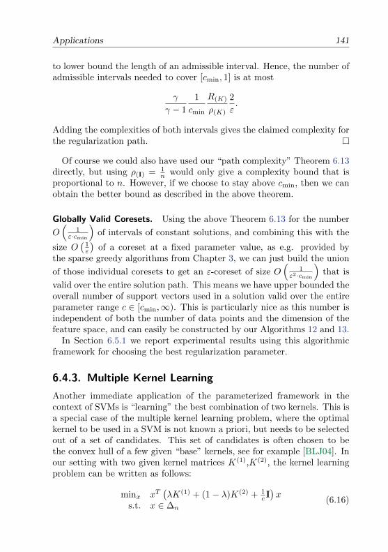
Applications 141
to lower bound the length of an admissible interval. Hence, the number ofadmissible intervals needed to cover [cmin, 1] is at most
γ
γ − 1
1
cmin
R(K)
ρ(K)
2
ε.
Adding the complexities of both intervals gives the claimed complexity forthe regularization path.
Of course we could also have used our “path complexity” Theorem 6.13directly, but using ρ(I) = 1
n would only give a complexity bound that isproportional to n. However, if we choose to stay above cmin, then we canobtain the better bound as described in the above theorem.
Globally Valid Coresets. Using the above Theorem 6.13 for the number
O(
1ε·cmin
)of intervals of constant solutions, and combining this with the
size O(
1ε
)of a coreset at a fixed parameter value, as e.g. provided by
the sparse greedy algorithms from Chapter 3, we can just build the union
of those individual coresets to get an ε-coreset of size O(
1ε2·cmin
)that is
valid over the entire solution path. This means we have upper bounded theoverall number of support vectors used in a solution valid over the entireparameter range c ∈ [cmin,∞). This is particularly nice as this number isindependent of both the number of data points and the dimension of thefeature space, and can easily be constructed by our Algorithms 12 and 13.
In Section 6.5.1 we report experimental results using this algorithmicframework for choosing the best regularization parameter.
6.4.3. Multiple Kernel Learning
Another immediate application of the parameterized framework in thecontext of SVMs is “learning” the best combination of two kernels. This isa special case of the multiple kernel learning problem, where the optimalkernel to be used in a SVM is not known a priori, but needs to be selectedout of a set of candidates. This set of candidates is often chosen to bethe convex hull of a few given “base” kernels, see for example [BLJ04]. Inour setting with two given kernel matrices K(1),K(2), the kernel learningproblem can be written as follows:
minx xT(λK(1) + (1− λ)K(2) + 1
c I)x
s.t. x ∈ ∆n(6.16)
142 Solution Paths for Convex Optimization Problems over Vectors
where 0 ≤ λ ≤ 1, is the parameter that we want to learn. To simplify
the notation, let us define the matrices K(1)c := K(1) + 1
c and K(2)c :=
K(2) + 1c . By scaling the objective function by 1/λ (where λ is assumed
to be non-zero), problem (6.16) can be transformed to a special case ofproblem (6.13), where t = 1−λ
λ (note again that the scaling does not affectour measure of primal-dual approximation error, because the error measureis relative):
minx xTK(1)c x+ t · xTK(2)
c xs.t. x ∈ ∆n
(6.17)
This again allows us to apply both approximation path Algorithms 12and 13, and to conclude from Theorem 6.13 that the complexity of anε-approximate path for problem (6.17) for t ∈ [0,∞] is in O
(1ε
). Here the
assumption that the distance problems associated to K(1)c and K
(2)c are
both separable holds trivially because 1/c > 0.
In the case that we have more than two base kernels we can still apply theabove approach if we fix the weights of all kernels except one. We can thennavigate along the solution paths optimizing each kernel weight separately,and therefore try to find total weights with a hopefully best possible cross-validation accuracy. Cross-validation refers to using splitting the availabledata into two disjoint sets, the training and the test set. The training setis used to obtain the model x (by solving the optimization problem), andlater the separate test set is used to validate the quality of the model x.
In Section 6.5.2 we report experimental results to determine the bestcombination of two kernels to achieve the highest prediction accuracy.
6.4.4. Minimum Enclosing Ball of Points under LinearMotion
The framework described here can also be used to solve the smallest en-closing ball problem for points in Rd that exhibit a linear motion in time,see [GJL10, GJL12a]. Here our algorithm improves the size of a coresetthat is valid at all time-points to O( 1
ε2 ), where the previous upper bound
was 2O( 1ε2
log 1ε ) due to [AHPY07], or O(1/ε2d) for maintaining the more
informative extent measures of the moving points [AHPV04].
Experimental Results 143
6.5. Experimental Results
The parameterized framework from Section 6.3 is also useful in practice.For support vector machines and multiple kernel learning, we have imple-mented the approximation path Algorithms 12 and 13 in Java. As theinternal optimizer, we used the sparse greedy Algorithm 3 as describedin Chapters 2 and 3. This algorithm can be implemented in a straight-forward way to work directly with the kernel matrix, without requiring ex-plicit representations of the datapoints in the kernel-space. We have seenin Chapter 5 that the method coincides with Gilbert’s algorithm [Gil66]in the geometric setting. In our implementations, we have also used thealternative MDM [MDM74] variant, also directly applied to the kernelmatrix.
We have tested our implementations on the following standard binaryclassification datasets (n points originally living in Rd each) from the UCIrepository2: ionosphere (n = 280, d = 34), breast-cancer (n = 546, d = 10),and MNIST 4k (n = 4000, d = 780). The timings were obtained by oursingle-threaded Java 6 implementation of MDM, using kernels (and nocaching of kernel evaluations), on an Intel C2D 2.4 GHz processor.
6.5.1. The Regularization Path of Support VectorMachines
Using the SVM formulation of problem (6.15) (for the `2-SVM withoutoffset), we compute approximate regularization paths for c ∈ [cmin =
1100000 , cmax = 100000] using the polynomial kernel (〈pi, pj〉 + 1)2. Asexperimental results we report in Table 6.1 the following quantities: (a)the time Tinit (in seconds) needed to compute an initial ε
γ -approximate
solution as the starting point, (b) the time Tpath (in seconds) needed tofollow the entire ε-approximate regularization path, when starting fromthe initial solution, (c) for comparison the time T3 (in seconds) neededto compute a static ε-approximate solution at the three fixed parametervalues c = cmin, 1 and cmax, and (d) the path complexity, i.e. the number#int of obtained admissible parameter intervals of constant ε-approximatesolutions along the path. The lower part of the table demonstrates the de-pendency of the path complexity on the choice of the parameter γ.
These experimental results show that the path complexity is indeed
2All datasets are available from www.csie.ntu.edu.tw/˜ cjlin/libsvmtools/datasets. Inour experiments, all features were scaled to [-1,1]. For MNIST, the first 5000 ’one’or ’seven’ images of the original dataset were used.
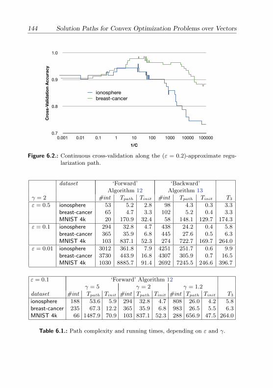
144 Solution Paths for Convex Optimization Problems over Vectors
0.7
0.8
0.9
1.0
0.001 0.01 0.1 1 10 100 1000 10000 100000
Cro
ss-V
alid
ati
on
Ac
cu
rac
y
1/C
ionospherebreast-cancer
Figure 6.2.: Continuous cross-validation along the (ε = 0.2)-approximate regu-larization path.
dataset ‘Forward’ ‘Backward’Algorithm 12 Algorithm 13
γ = 2 #int Tpath Tinit #int Tpath Tinit T3
ε = 0.5 ionosphere 53 5.2 2.8 98 4.3 0.3 3.3breast-cancer 65 4.7 3.3 102 5.2 0.4 3.3MNIST 4k 20 170.9 32.4 58 148.1 129.7 174.3
ε = 0.1 ionosphere 294 32.8 4.7 438 24.2 0.4 5.8breast-cancer 365 35.9 6.8 445 27.6 0.5 6.3MNIST 4k 103 837.1 52.3 274 722.7 169.7 264.0
ε = 0.01 ionosphere 3012 361.8 7.9 4251 251.7 0.6 9.9breast-cancer 3730 443.9 16.8 4307 305.9 0.7 16.5MNIST 4k 1030 8885.7 91.4 2692 7245.5 246.6 396.7
ε = 0.1 ‘Forward’ Algorithm 12γ = 5 γ = 2 γ = 1.2
dataset #int Tpath Tinit #int Tpath Tinit #int Tpath Tinit T3
ionosphere 188 53.6 5.9 294 32.8 4.7 808 26.0 4.2 5.8breast-cancer 235 67.3 12.2 365 35.9 6.8 983 26.5 5.5 6.3MNIST 4k 66 1487.9 70.9 103 837.1 52.3 288 656.9 47.5 264.0
Table 6.1.: Path complexity and running times, depending on ε and γ.
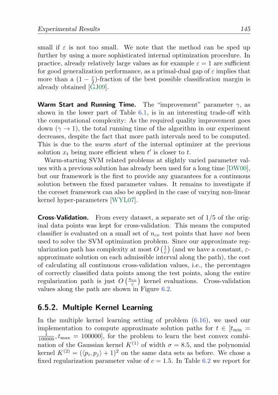
Experimental Results 145
small if ε is not too small. We note that the method can be sped upfurther by using a more sophisticated internal optimization procedure. Inpractice, already relatively large values as for example ε = 1 are sufficientfor good generalization performance, as a primal-dual gap of ε implies thatmore than a (1 − ε
2 )-fraction of the best possible classification margin isalready obtained [GJ09].
Warm Start and Running Time. The “improvement” parameter γ, asshown in the lower part of Table 6.1, is in an interesting trade-off withthe computational complexity: As the required quality improvement goesdown (γ → 1), the total running time of the algorithm in our experimentdecreases, despite the fact that more path intervals need to be computed.This is due to the warm start of the internal optimizer at the previoussolution xt being more efficient when t′ is closer to t.
Warm-starting SVM related problems at slightly varied parameter val-ues with a previous solution has already been used for a long time [DW00],but our framework is the first to provide any guarantees for a continuoussolution between the fixed parameter values. It remains to investigate ifthe coreset framework can also be applied in the case of varying non-linearkernel hyper-parameters [WYL07].
Cross-Validation. From every dataset, a separate set of 1/5 of the orig-inal data points was kept for cross-validation. This means the computedclassifier is evaluated on a small set of ncv test points that have not beenused to solve the SVM optimization problem. Since our approximate reg-ularization path has complexity at most O
(1ε
)(and we have a constant, ε-
approximate solution on each admissible interval along the path), the costof calculating all continuous cross-validation values, i.e., the percentagesof correctly classified data points among the test points, along the entireregularization path is just O
(ncvε
)kernel evaluations. Cross-validation
values along the path are shown in Figure 6.2.
6.5.2. Multiple Kernel Learning
In the multiple kernel learning setting of problem (6.16), we used ourimplementation to compute approximate solution paths for t ∈ [tmin =
1100000 , tmax = 100000], for the problem to learn the best convex combi-
nation of the Gaussian kernel K(1) of width σ = 8.5, and the polynomialkernel K(2) = (〈pi, pj〉+ 1)2 on the same data sets as before. We chose afixed regularization parameter value of c = 1.5. In Table 6.2 we report for
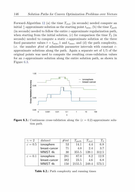
146 Solution Paths for Convex Optimization Problems over Vectors
Forward-Algorithm 12 (a) the time Tinit (in seconds) needed compute aninitial εγ -approximate solution as the starting point tmin, (b) the time Tpath(in seconds) needed to follow the entire ε-approximate regularization path,when starting from the initial solution, (c) for comparison the time T3 (inseconds) needed to compute a static ε-approximate solution at the threefixed parameter values t = tmin, 1 and tmax, and (d) the path complexity,i.e. the number #int of admissible parameter intervals with constant ε-approximate solutions along the path. Again a separate set of 1/5 of theoriginal points was used to compute the resulting cross-validation valuesfor an ε-approximate solution along the entire solution path, as shown inFigure 6.3.
0.85
0.90
0.95
1.00
0 0.001 0.01 0.1 1 10 100
Cro
ss-V
alid
ati
on
Ac
cu
rac
y
t
ionospherebreast-cancer
Figure 6.3.: Continuous cross-validation along the (ε = 0.2)-approximate solu-tion path.
γ = 2 dataset #int Tpath Tinit T3
ε = 0.5 ionosphere 53 14.1 4.4 6.8breast-cancer 71 4.0 2.4 3.7MNIST 4k 30 355.5 139.1 312.5
ε = 0.1 ionosphere 281 87.0 8.2 12.9breast-cancer 382 23.5 4.6 6.8MNIST 4k 150 2155.5 249.4 573.5
Table 6.2.: Path complexity and running times
Conclusion 147
In practice, there are related methods that optimize a joint objectivefunction over both the classifier weights and the combination of multiplekernels [BLJ04, RBCG08]. These methods are experimentally fast, butare not directly comparable to ours as they do not obtain a solution pathand are therefore unable to provide guarantees such as an optimal cross-validation value along a parameter path.
6.6. Conclusion
We have presented a framework to optimize convex functions over theunit simplex that are parameterized by an additional parameter. Thisallows us to maintain a guaranteed approximation quality along the entirecontinuous solution path, by piecewise constant solutions. Also, for manypractical cases, we can efficiently compute the exact interval length overwhich a solution stays valid, allowing to adapt to the local shape of theoptimization function in the parameter. The framework is general, simpleand has been proven to be practical on a number of machine learningproblems.

7Solution Paths for
Semidefinite Optimization
We devise a framework for computing an approximate solution path for animportant class of parameterized semidefinite problems that is guaranteedto be ε-close to the exact solution path. As a result, we can compute theentire regularization path for most matrix completion and factorizationapproaches, as well as nuclear norm or weighted nuclear norm regularizedconvex optimization problems. This also includes robust PCA and variantsof sparse PCA and maximum variance unfolding. On the theoretical side,we show that the complexity of the approximate path is independent ofthe size of the input matrix. More precisely, the path complexity onlygrows linearly with the inverse of the desired approximation quality ε, andwith the model complexity (regularization). This implies that the wholesolution path can be computed in near linear time in the size of the input.Our experiments demonstrate the practical efficiency of the approach forlarge matrix completion problems.
This chapter is joint work with Joachim Giesen and Soeren Laue [GJL12b],and generalizes the path method from the previous Chapter 6 to the caseof semidefinite optimization over bounded trace.
149
150 Solution Paths for Semidefinite Optimization
7.1. Introduction
We provide an algorithmic framework for tracking approximate solutionsof parameterized semidefinite optimization problems along the parameterpath. The algorithm is very simple and comes with strong guarantees onthe approximation quality (continuously along the path) as well as therunning time. The idea of our scheme is the same as in the previousChapter 6: We compute at a parameter value an approximate solutionthat is slightly better than the required quality, and then keep this solutionas the parameter changes, exactly as long as the required approximationquality can still be guaranteed. Only when the approximation quality isno longer sufficient, a new solution needs to be computed. As alreadyin the vector case in Chapter 6, we prove that the number of necessaryupdates along the entire path is only O
(1ε
), if an approximation guarantee
of ε > 0 is required along the path. The path complexity therefore againis independent of the size of the problem (number of variables).
The task of considering and computing the entire path of (near) optimalsolutions to parameterized problems appears naturally in various differentfields, such as control theory, various multi-objective optimization applica-tions, and most notably from regularization methods in machine learning.The question of parameter selection — e.g. the choice of the best reg-ularization parameter — is often a non-trivial task. Many approacheshave been proposed in the last decade for tracking exact solution pathsfor vector optimization problems, in the case that the paths are piecewiselinear. However there are many applications where this assumption doesnot hold, and even if it does, the path might have exponential complexityin the worst case [GJM10]. Our new framework strongly contrasts the ex-isting approaches in the literature, and proves a path complexity of O
(1ε
)for a wider class of problems.
Again as in Chapter 6, our framework here is not tied to a specific algo-rithm, and very simple to implement: Any existing semidefinite optimizeror heuristic of choice can be used to compute an approximate solution atfixed parameter values. We only need to compute a bound on the dualitygap for a given candidate at a fixed parameter value, in order to be able toapply our path framework. We show that the duality gap can efficientlybe computed by a single eigenvalue computation. Despite the frameworkbeing very simple, we demonstrate that it is well applicable for practicallarge scale problems. Furthermore, as we have already argued for vec-tor optimization problems, the path complexity of O
(1ε
)is indeed best
possible in the worst case.
Introduction 151
Our experiments demonstrate that often, the computation of an entireε-approximate solution path is only marginally more expensive than thecomputation of a single approximate solution.
Parameterized Semidefinite Optimization. Our goal is to compute theentire solution path (with a continuously guaranteed approximation qual-ity) for parameterized semidefinite problems over bounded trace, i.e. op-timization problems of the form (3.5)
minX
ft(X)
s.t. Tr(X) = 1 ,X 0 ,
(7.1)
or the analogous inequality-constrained variant
minX
ft(X)
s.t. Tr(X) ≤ 1 ,X 0 ,
(7.2)
where ft is a family of convex functions, parameterized by t ∈ R, definedon symmetric matrices X ∈ Sn×n. We are in particular interested in thespecial case where the parameterization is given by the trace itself, i.e.
minX
f(X)
s.t. Tr(X) ≤ t ,X 0 .
(7.3)
All three formulations have prominent applications in various areas.Clearly the last formulation can be seen as a special case of (7.2), for thefunction ft(X) := f(tX) that re-scales its argument. Furthermore (7.2) isa special case of (7.1), as we can always add an additional slack row/column(of which the function does not depend) to the matrix.
Motivation and Applications. Our work is motivated by nuclear normregularized optimization problems, see also Chapter 4, which have be-come central to many applications in machine learning and compressedsensing, as for example low-rank recovery [FHB01, CR09, CT10], robustPCA [CLMW11], and matrix completion [SRJ04, RS05, Web06, Lin07,KBV09, TPNT09, SS10]. Formally we study problems of the form
minZ∈Rm×n
f(Z) + λ ‖Z‖∗ (7.4)
152 Solution Paths for Semidefinite Optimization
for a convex function f (the loss function), where ‖.‖∗ is the nuclear norm.We recall that the equivalent constrained formulation (4.2) is
minZ∈Rm×n, ‖Z‖∗≤ t/2
f(Z) . (7.5)
Both problems are parameterized by a real regularization parameter (λand t respectively). Note that the former is the Lagrangian formulation ofthe latter.
To relate the above nuclear norm regularized problems (7.4) and (7.5)to semidefinite optimization, the straightforward transformation that weexplained in Section 4.4 (or see e.g. [FHB01, SRJ04, JS10]) comes to help.This along the way also explains why the nuclear norm is widely called thetrace norm: Any problem of the form (7.5) is equivalent to optimizing the
semidefinite version (7.3) for a function f : S(m+n)×(m+n) → R, where fis defined as
f(X) = f
((V ZZT W
)):= f(Z) (7.6)
for Z ∈ Rm×n being the upper right part of X. Formally we again thinkof the variable X ∈ S(m+n)×(m+n) as consisting of the four parts X =:(V ZZT W
)with V ∈ Sm×m,W ∈ Sn×n and Z ∈ Rm×n. Observe that f is
convex whenever f is convex.
Related Work. For kernel methods and many other machine learningtechniques, the resulting optimization problems often turn out to be pa-rameterized convex quadratic programs, and in recent years a plenitude ofalgorithms and heuristics have been developed to “track” these solutionpaths, see e.g. [HRTZ04, LGC07, RZ07, LS07, PH07]. However, the exactpiecewise linear solution path of parameterized quadratic programs (in par-ticular for the SVM) is known to be of exponential complexity in the worstcase [GJM10]. In the work here by contrast we show that just constantlymany intervals of the parameter are sufficient for any fixed desired contin-uous approximation quality ε > 0. For vector optimization problems suchas SVMs, we have described in the previous Chapter 6 on how guaranteesalong the entire path can be obtained, see also [GJL10, GJL12a].
To our best knowledge, no path algorithms were known so far for themore general case of semidefinite optimization. The solution path forsparse principal component analysis (PCA) was investigated by [dBG07],which however is parameterized over discrete integral values from 1 to n,where n is the number of variables. For a variant of low-rank matrix com-pletion, [MHT10] suggest to perform a grid search on the regularization
The Duality Gap 153
parameter interval, computing a single approximate solution at each pa-rameter t. However, they provide no approximation guarantee betweenthe chosen grid points.
7.2. The Duality Gap
In this small section we will briefly recall the practical approximation qual-ity measures for convex optimization problems of the form (7.1), (7.2)or (7.3), which we have discussed in more detail in Section 3.4. For thiswe will assume that our objective function ft(X) is continuously differen-tiable1. We consider the gradient ∇ft(X) with respect to X, which is asymmetric matrix in Sn×n.
We write X • Y for the entry-wise inner product of two matrices.
Lemma 7.1. The duality gap at any matrix X ∈ Sn×n is given by thedifference of ft(X) to its corresponding dual value ωt(X), and equals
gt(X) = λmax (−∇ft(X)) +X • ∇ft(X) for problem (7.1),
gt(X) = max 0, λmax (−∇ft(X))+X • ∇ft(X) for problem (7.2),
gt(X) = t ·max 0, λmax (−∇f(X))+X •∇f(X) for problem (7.3).
Furthermore, it holds that ft(X)− ft(X∗) ≤ gt(X) for any feasible X, forX∗ being an optimal solution to the respective optimization problem.
Proof. We have calculated the duality gap for problem (7.1) in equa-tion (3.6) in Section 3.4, using the fact that the spectahedron domainS := X ∈ Sn×n |X 0, Tr(X) = 1 is the convex hull of the rank-1 ma-trices of unit trace. The expressions for the later two problem variantsthen follow from the same result, because both problems can be reducedto the first formulation (7.1) as described above.
The last mentioned fact makes the duality gap an extremely usefulmeasure of approximation and stopping criterion for practical optimiz-ers: While the optimum value ft(X
∗) is usually unknown, the gap gt(X)readily guarantees a simple upper bound on the current difference to thisoptimum value. For all variants, the quantity gt is easily computable forany candidate solution X even for very large problems, as we only need
1If ft(X) is convex but not differentiable, the concepts of standard Lagrange dualitycan be still generalized for subgradients analogously, so that any element of thesubgradient will give an upper bound on the approximation error, see Chapter 2.
154 Solution Paths for Semidefinite Optimization
to perform a single eigenvalue computation, assumed that the gradient isavailable.
Having these nice mentioned properties, one would think that the achievedduality gap is the standard or routine measure when comparing differentheuristics for the same optimization problems. However, in the currentmachine learning literature, this is not yet done as often as one wouldwish.
As explained in Chapter 2, the duality gap gt can also be interpretedas the difference of the function value to the minimum value of the linearapproximation to f at point X, where the minimum is taken over thefeasible region. Alternatively, the above Lemma can also be obtained fromstandard duality theory [BV04, Section 5.9] or [Haz08].
Definition 7.2. Let ε > 0. A matrix X ∈ Sn×n that is feasible for oneof the above optimization problems at some parameter value t is called anε-approximation if the duality gap satisfies
gt(X) ≤ ε .
7.3. Optimizing Parameterized SemidefiniteProblems
We are interested in ε-approximations for problems (7.1), (7.2) and (7.3)for all valid parameter values t ∈ R, and will study the complexity of suchsolution paths in the following. This definition coincides with the measurewe used for vector problems in Chapter 6.
Definition 7.3. The ε-approximation path complexity of a parameterizedoptimization problem is defined as the minimum number of intervals overall possible partitions of the parameter range [tmin, tmax] ⊂ R, such that foreach individual interval, there is a single solution that is an ε-approximationfor that entire interval.
General Parameterized Functions. The following simple lemma is at thecore of our discussion of approximation paths, and characterizes how farwe can change the parameter t such that a given ε
γ -approximate solution
X (for γ > 1) at t stays an ε-approximate solution.
Lemma 7.4 (Stability of an Approximation). Let X be an εγ -approximation
to problem (7.1) for some fixed parameter value t, and for some γ > 1.
Optimizing Parameterized Semidefinite Problems 155
Then for all parameters t′ ∈ R and feasible X ′ that satisfy
λmax (−∇ft′(X ′))− λmax (−∇ft(X))
+ X ′ • ∇ft′(X ′) − X • ∇ft(X) ≤ ε(
1− 1γ
),
(7.7)
it holds that X ′ is an ε-approximation to problem (7.1) at the changedparameter value t′.
Proof. In the equality constrained case, we have to show that gt′(X′) =
λmax (−∇ft′(X ′)) + X ′ • ∇ft′(X ′) ≤ ε. To do so, we add to the inequal-ity (7.7) the inequality stating that X is an ε
γ -approximate solution atvalue t, i.e.
λmax (−∇ft(X)) +X • ∇ft(X) ≤ ε
γ,
to obtain the claimed bound on the gap at the new parameter value t′.
The above Lemma 7.4 does also apply for the inequality-constrainedcase (7.2), if we just replace the two λmax(.)-terms in condition (7.7) bymax 0, λmax(.) instead. The proof follows analogously. Alternatively,this change can also be seen by adding a slack row/column to X, andtherefore reducing to the equality constrained case (7.1).
The following alternative (more restrictive) criterion is simpler to eval-uate in a concrete implementation of our path algorithms, as for examplefor more complicated parameterizations of (7.1) or (7.2).
Lemma 7.5. Let X be an εγ -approximation for problem (7.1) or (7.2) for
some fixed parameter value t, and for some γ > 1. Then for all t′ ∈ R thatsatisfy
(1 + ‖X‖Fro) ‖∇ft′(X)−∇ft(X)‖Fro ≤ ε(
1− 1
γ
),
it holds that X is still an ε-approximation at parameter value t′.
Proof. We aim to apply Lemma 7.4, and therefore try to upper boundthe terms on the left hand side of inequality (7.7) for X ′ = X. We startby upper bounding the difference in the λmax-values: Weyl’s perturbationtheorem on the eigenvalues of a matrix A′ = A+ E states that
|λmax(A′)− λmax(A)| ≤ ‖E‖spec .
See e.g. [Nak10]. The matrix spectral norm always satisfies ‖E‖spec ≤‖E‖Fro. Applying Weyl’s theorem to A′ = −∇ft′(X) and A = −∇ft(X)
156 Solution Paths for Semidefinite Optimization
gives|λmax (−∇ft′(X))− λmax (−∇ft(X))|≤ ‖∇ft′(X)−∇ft(X)‖Fro .
(7.8)
It remains to upper bound the term X • (∇ft′(X)−∇ft(X)), which canbe done by using the Cauchy-Schwarz inequality
|X • (∇ft′(X)−∇ft(X))| ≤ ‖X‖Fro · ‖∇ft′(X)−∇ft(X)‖Fro .Hence, the inequality in the assumption of this lemma implies that in-equality (7.7) in Lemma 7.4 holds, with X ′ = X, from which we obtainour claimed approximation quality gt′(X) ≤ ε for the equality constrainedProblem (7.1).
For the inequality constrained case of Problem (7.2), the same resultfollows since the bound (7.8) that we obtained from Weyl’s theorem inparticular also implies that
|max 0, λmax (−∇ft′(X)) −max 0, λmax (−∇ft(X))|≤ ‖∇ft′(X)−∇ft(X)‖Fro .
This follows by observing that |max0, a −max0, b| ≤ |a− b|. Thismeans we have the desired bound on the approximation quality at t′ alsofor the duality gap for problem version (7.2).
For the following main theorem on the path complexity, we again assumethat the global parameter range of interest, [tmin, tmax] ⊂ R, is finite.
Theorem 7.6. Let ft be convex and continuously differentiable in X, andlet ∇ft(X) be Lipschitz continuous in t, for all feasible X. Then the ε-approximation path complexity of problems (7.1) and (7.2) over the pa-rameter range t ∈ [tmin, tmax] ⊂ R is in O
(1ε
).
Proof. In order for the condition of Lemma 7.5 to be satisfied, we first usethat for any X 0,Tr(X) ≤ 1,
(1 + ‖X‖Fro) ‖∇ft′(X)−∇ft(X)‖Fro≤ (1 + ‖X‖Fro) · L · |t′ − t|≤ 2 · L · |t′ − t| .
Here L is the supremum of the Lipschitz constants w.r.t. t of the derivatives∇ft(X), taken over the compact feasible domain for X. So if we require the
intervals to be of length |t′ − t| ≤ ε2L
(1− 1
γ
), we have that the condition
in Lemma 7.5 is satisfied for any X 0,Tr(X) ≤ 1.Dividing the total parameter range |tmax − tmin| by this interval length
of ε2L
(1− 1
γ
), the bound on the path complexity follows directly.
Optimizing Parameterized Semidefinite Problems 157
Optimality. This path complexity result is in fact best possible. When∇ft(X) does effectively change with t with rate LX (here LX is the Lips-chitz constant w.r.t. t of ∇ft(X)), then the interval length where gt(X) ≤ε holds can not be longer than Θ(ε). For an explicit example of a functionresulting in this worst-case complexity, we refer to our discussion for thevector case in Section 6.3.3. To adapt this to the case of trace one matri-ces, one can consider the analogous linear function ft(X) := X •H(t), forH(t) := diag(h(t)) being diagonal.
Optimizing with Growing Trace. In the special case of problem (7.3),the calculation of the lengths of intervals of guaranteed ε-approximationquality becomes considerably simpler:
Lemma 7.7. Let X be an εγ -approximate solution of problem (7.3) for some
fixed parameter value t, and for some γ > 1. Then for all t′ ≥ t ∈ R thatsatisfy
(t′ − t) · λmax (−∇f(X)) ≤ ε(
1− 1γ
), (7.9)
the solution X is still an ε-approximation to problem (7.3) at the parametervalue t′.
Proof. Follows from Lemma 7.4 applied to the function ft(X′) := f(tX ′),
if we set the new approximation to X ′ := tt′X. An alternative direct proof
also goes along the same lines as in Lemma 7.4.
7.3.1. Computing Approximate Solution Paths
The above Lemmata 7.4 and 7.7 on “preserving the approximation quality”do immediately suggest two simple algorithms to compute ε-approximatesolution paths, which are depicted in Algorithms 14 and 15. Furthermore,they imply that we can efficiently and locally compute the exact largestpossible interval length for each given pair (X, t) in practice. In thoseregions where f changes only slowly in t, this makes the algorithms muchmore efficient than if we would just work with the guaranteed O(ε) worst-case upper bound on the interval lengths.
By Theorem 7.6 (or Lemma 7.7 respectively), the running time of thismethod is O(T ( εγ )/ε), where T (ε′) is the time to compute a single ε′-approximate solution for problem (7.1), (7.2) or (7.3) at a fixed parametervalue.
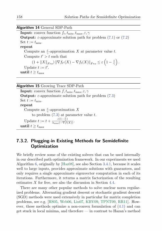
158 Solution Paths for Semidefinite Optimization
Algorithm 14 General SDP-Path
Input: convex function ft, tmin, tmax, ε, γOutput: ε-approximate solution path for problem (7.1) or (7.2)Set t := tmin.repeat
Compute an εγ -approximation X at parameter value t.
Compute t′ > t such that
(1 + ‖X‖Fro) ‖∇ft′(X)−∇ft(X)‖Fro ≤ ε(
1− 1γ
).
Update t := t′.until t ≥ tmax
Algorithm 15 Growing Trace SDP-Path
Input: convex function f, tmin, tmax, ε, γOutput: ε-approximate solution path for problem (7.3)Set t := tmin.repeat
Compute an εγ -approximation X
to problem (7.3) at parameter value t.
Update t := t+ε(1− 1
γ )
λmax(−∇f(X)) .
until t ≥ tmax
7.3.2. Plugging-in Existing Methods for SemidefiniteOptimization
We briefly review some of the existing solvers that can be used internallyin our described path optimization framework. In our experiments we usedAlgorithm 6, originally by [Haz08], see also Section 3.4.1, because it scaleswell to large inputs, provides approximate solutions with guarantees, andonly requires a single approximate eigenvector computation in each of itsiterations. Furthermore, it returns a matrix factorization of the resultingestimates X for free, see also the discussion in Section 4.4.
There are many other popular methods to solve nuclear norm regular-ized problems. Alternating gradient descent or stochastic gradient descent(SGD) methods were used extensively in particular for matrix completionproblems, see e.g. [RS05, Web06, Lin07, KBV09, TPNT09, RR11]. How-ever, these methods optimize a non-convex formulation of (4.1) and canget stuck in local minima, and therefore — in contrast to Hazan’s method
Applications 159
with our convex transformation (7.6) — come with no convergence guaran-tee. On the other hand, there are also several known convex optimizationmethods of “proximal gradient” and “singular value thresholding”-typefrom the optimization community, see e.g. [TY10], which however experi-mentally perform slower than Hazan’s method [JS10].
Nevertheless, any of these other methods and heuristics can still beused as the internal optimizer in our path-following framework, as we canalways compute the duality gap as a certificate for the quality of the foundapproximate solution.
7.4. Applications
Using our above path approximation framework, we directly obtain piece-wise constant solution paths of guaranteed approximation quality for anyproblem of the form (7.1), (7.2) or (7.3), including all nuclear norm reg-ularized problems (7.4) and (7.5), such as standard matrix completionproblems, which we introduce next.
7.4.1. Matrix Completion
Our path framework applies to matrix completion problems with any con-vex differentiable loss function, such as the smoothed hinge loss or thestandard squared loss, and includes the classical maximum-margin matrixfactorization variants [SRJ04].
The regularized matrix completion task is exactly problem (7.5) wherethe function f is given by the loss over the observed entries of the matrix,Ω ⊆ [n]× [m], i.e. f(Z) =
∑(i,j)∈Ω L(Zij , Yij). Here L(., .) is an arbitrary
loss-function that is convex in its Z-argument. By far the most widelyused variant employs the squared loss, given by
f(Z) =1
2
∑(i,j)∈Ω
(Zij − Yij)2. (7.10)
Using the notation (A)Ω for the matrix that coincides with A on the indicesΩ and is zero otherwise, ∇f(Z) can be written as
∇f(Z) = (Z − Y )Ω .
This implies that the symmetric gradient matrix ∇f(X) ∈ S(m+n)×(m+n)
for our transformed problem (7.6) that we use in our algorithm is also
160 Solution Paths for Semidefinite Optimization
of this simple form (recall the notation X =(V ZZT W
)). As this matrix
is sparse — it has only |Ω| non-zero entries — storage and approximateeigenvector computations can be performed much more efficiently than fordense problems. An equivalent matrix factorization of any approximationX for problem (7.3) can always be obtained directly from the Choleskydecomposition of X, because X 0.
7.4.2. Solution Paths for the Weighted Nuclear Norm
We recall from Section 4.2.1 that any convex problem with a constrainedweighted nuclear norm
minZ∈Rm×n, ‖Z‖nuc(p,q)≤ t/2
f(Z) (7.11)
is equivalent to a classical nuclear norm regularized problem
minZ∈Rm×n,‖Z‖∗≤ t/2
f(P−1ZQ−1).
(this corresponds to substituting Z := PZQ for some fixed diagonal ma-trices P,Q). Therefore the problem can be directly formulated in the formof (7.3), and our path tracking Algorithm 15 applies without modifications.
7.4.3. Solution Paths for Robust PCA
With principal component analysis (PCA) being today’s most widely usedtool for the analysis of high-dimensional data and dimensionality reduc-tion, but being very sensitive to errors and noise in just a single data-point, [CLMW11] have proposed the following robust version of PCA, alsocalled principal component pursuit
minZ∈Rm×n
‖Z‖∗ + λ′ ‖M − Z‖1 .
Here ‖.‖1 is the entry-wise `1-norm, and M ∈ Rm×n is the given datamatrix. This problem is already of the form (7.4), for λ = 1
λ′ . Thereforewe can obtain the entire path in the nuclear norm regularization parameterλ, and the corresponding constrained variant (7.5), by using our simpleAlgorithm 15 for growing trace.
As the internal optimizer, any existing method for robust PCA can beused. If the ‖.‖1-norm is smoothened (see also Section 4.5.1), then thesame stopping criterion determined by the duality gap from Lemma 7.1
Applications 161
applies. Alternatively, if the original non-smooth formulation (7.5) overthe domain
Z ∈ Rm×n
∣∣ ‖Z‖∗ ≤ t2
is solved approximately by some ar-
bitrary optimizer, then we can use our generalization of the duality gapto the case of non-smooth functions, see Section 2.2. In this case, anysubgradient DZ of our objective function ‖M − Z‖1 gives a certificate forsome value of a duality gap g(Z,DZ) as defined in equation (2.5).
We therefore obtain piecewise constant solutions together with a con-tinuous ε-approximation guarantee along the entire regularization path.
7.4.4. Solution Paths for Sparse PCA and MaximumVariance Unfolding
Sparse PCA. The concept of sparse PCA is to approximate a given datamatrix A ∈ Sn×n by approximate eigenvectors that are additionally sparse,see [ZdG10] for an overview. Many algorithms have been proposed forsparse PCA, see e.g. [SB08] and [dBG07], the latter also considering thediscrete solution path, as the sparsity changes.
The SDP-relaxation of [dGJL07, Equation 3.2] for sparse PCA of amatrix A is given by
minX0
ρ · 1T |X|1− Tr(AX)
s.t. Tr(X) = 1 ,X 0 .
(7.12)
Here |X| is element-wise for the matrix X, and 1 ∈ Rn is the all-onevector. Using our path Algorithm 14, we can compute the approximatesolution path in the penalty parameter ρ of this relaxation, which is of theform (7.1).
Maximum Variance Unfolding. Another interesting technique for non-linear dimensionality reduction is named maximum variance unfolding(MVU). Here we consider the Laplacian regularized MVU formulation
minX0
∑i∼j
((QXQT )ii+(QWQT )jj−2(QXQT )ij−d2
ij
)2− 1
νTr(X) , (7.13)
see [WSZS07, Formulation (7)]. Here the notation i ∼ j means that thevertices i and j form an edge in the underlying graph. In this formulation,a previously fixed low-rank matrix Q is used to represent the local neigh-borhood structure of the graph, given by the bottom-most eigenvectors ofthe graph Laplacian. This directly fits into problem (7.3), therefore ourAlgorithm 15 applies for parameter 1
ν .
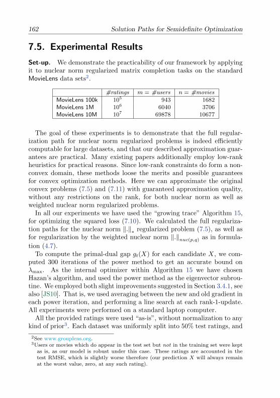
162 Solution Paths for Semidefinite Optimization
7.5. Experimental Results
Set-up. We demonstrate the practicability of our framework by applyingit to nuclear norm regularized matrix completion tasks on the standardMovieLens data sets2.
#ratings m = #users n = #movies
MovieLens 100k 105 943 1682MovieLens 1M 106 6040 3706MovieLens 10M 107 69878 10677
The goal of these experiments is to demonstrate that the full regular-ization path for nuclear norm regularized problems is indeed efficientlycomputable for large datasets, and that our described approximation guar-antees are practical. Many existing papers additionally employ low-rankheuristics for practical reasons. Since low-rank constraints do form a non-convex domain, these methods loose the merits and possible guaranteesfor convex optimization methods. Here we can approximate the originalconvex problems (7.5) and (7.11) with guaranteed approximation quality,without any restrictions on the rank, for both nuclear norm as well asweighted nuclear norm regularized problems.
In all our experiments we have used the “growing trace” Algorithm 15,for optimizing the squared loss (7.10). We calculated the full regulariza-tion paths for the nuclear norm ‖.‖∗ regularized problem (7.5), as well asfor regularization by the weighted nuclear norm ‖.‖nuc(p,q) as in formula-
tion (4.7).To compute the primal-dual gap gt(X) for each candidate X, we com-
puted 300 iterations of the power method to get an accurate bound onλmax. As the internal optimizer within Algorithm 15 we have chosenHazan’s algorithm, and used the power method as the eigenvector subrou-tine. We employed both slight improvements suggested in Section 3.4.1, seealso [JS10]. That is, we used averaging between the new and old gradient ineach power iteration, and performing a line search at each rank-1-update.All experiments were performed on a standard laptop computer.
All the provided ratings were used “as-is”, without normalization to anykind of prior3. Each dataset was uniformly split into 50% test ratings, and
2See www.grouplens.org.3Users or movies which do appear in the test set but not in the training set were kept
as is, as our model is robust under this case. These ratings are accounted in thetest RMSE, which is slightly worse therefore (our prediction X will always remainat the worst value, zero, at any such rating).
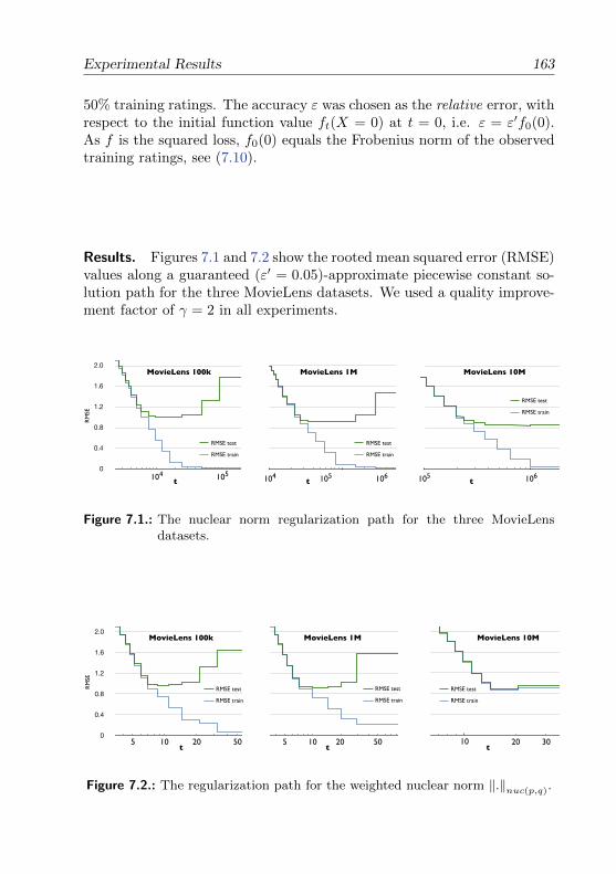
Experimental Results 163
50% training ratings. The accuracy ε was chosen as the relative error, withrespect to the initial function value ft(X = 0) at t = 0, i.e. ε = ε′f0(0).As f is the squared loss, f0(0) equals the Frobenius norm of the observedtraining ratings, see (7.10).
Results. Figures 7.1 and 7.2 show the rooted mean squared error (RMSE)values along a guaranteed (ε′ = 0.05)-approximate piecewise constant so-lution path for the three MovieLens datasets. We used a quality improve-ment factor of γ = 2 in all experiments.
0
0.4
0.8
1.2
1.6
2.0
1000 10000 1000000
0.4
0.8
1.2
1.6
2.0
10000 100000 10000000
0.4
0.8
1.2
1.6
2.0
100000 1000000 10000000
0
0.4
0.8
1.2
1.6
2.0
1 10 1000
0.4
0.8
1.2
1.6
2.0
1 10 1000
0.4
0.8
1.2
1.6
2.0
1 10 100
104 105 106
RMSE test
RMSE train
MovieLens 1M
t 105 1060
0.4
0.8
1.2
1.6
2.0
100000 1000000 10000000
0
0.4
0.8
1.2
1.6
2.0
1 10 100
RMSE test
RMSE train
MovieLens 10M
t104 1050
0.4
0.8
1.2
1.6
2.0
1000 10000 1000000
0.4
0.8
1.2
1.6
2.0
10000 100000 10000000
0.4
0.8
1.2
1.6
2.0
100000 1000000 10000000
0
0.4
0.8
1.2
1.6
2.0
1 10 1000
0.4
0.8
1.2
1.6
2.0
1 10 1000
0.4
0.8
1.2
1.6
2.0
1 10 100
Weighted nuclear norm
0
0.4
0.8
1.2
1.6
2.0
1000 10000 1000000
0.4
0.8
1.2
1.6
2.0
10000 100000 10000000
0.4
0.8
1.2
1.6
2.0
100000 1000000 10000000
0
0.4
0.8
1.2
1.6
2.0
1 10 1000
0.4
0.8
1.2
1.6
2.0
1 10 1000
0.4
0.8
1.2
1.6
2.0
1 10 100
Weighted nuclear norm
RMSE test
RMSE train
MovieLens 100k
t
RM
SE
Figure 7.1.: The nuclear norm regularization path for the three MovieLensdatasets.
0
0.4
0.8
1.2
1.6
2.0
1000 10000 1000000
0.4
0.8
1.2
1.6
2.0
10000 100000 10000000
0.4
0.8
1.2
1.6
2.0
100000 1000000 10000000
0
0.4
0.8
1.2
1.6
2.0
1 10 1000
0.4
0.8
1.2
1.6
2.0
1 10 1000
0.4
0.8
1.2
1.6
2.0
1 10 100
Weighted nuclear norm
10 205 50
RMSE test
RMSE train
MovieLens 1M
t
0
0.4
0.8
1.2
1.6
2.0
1000 10000 1000000
0.4
0.8
1.2
1.6
2.0
10000 100000 10000000
0.4
0.8
1.2
1.6
2.0
100000 1000000 10000000
0
0.4
0.8
1.2
1.6
2.0
1 10 1000
0.4
0.8
1.2
1.6
2.0
1 10 1000
0.4
0.8
1.2
1.6
2.0
1 10 100
Weighted nuclear norm
0
0.4
0.8
1.2
1.6
2.0
1000 10000 1000000
0.4
0.8
1.2
1.6
2.0
10000 100000 10000000
0.4
0.8
1.2
1.6
2.0
100000 1000000 10000000
0
0.4
0.8
1.2
1.6
2.0
1 10 1000
0.4
0.8
1.2
1.6
2.0
1 10 1000
0.4
0.8
1.2
1.6
2.0
1 10 100
Weighted nuclear norm
10 205 50
RMSE test
RMSE train
MovieLens 100k
t
RM
SE
0
0.4
0.8
1.2
1.6
2.0
1 10 10010 30
RMSE test
RMSE train
MovieLens 10M
t20
Figure 7.2.: The regularization path for the weighted nuclear norm ‖.‖nuc(p,q).
164 Solution Paths for Semidefinite Optimization
Table 7.1.: Dependency of the path complexity (#int) on the accuracy ε.
Regularization Accuracy MovieLens 100k, γ = 2ε/f0(0) tmin tmax #int ∆avg
t f traintmax
f testopt
Nuclear norm 0.05 1000 60000 21 4515 0.0150 0.9912‖.‖∗ 0.01 1000 60000 97 582 0.0054 0.9905
0.002 1000 60000 386 175 0.0009 0.9981
Weighted 0.05 2 50 17 3.21 0.0619 0.9607nuclear norm 0.01 2 50 72 1.18 0.0147 0.9559‖.‖nuc(p,q) 0.002 2 50 325 0.140 0.0098 0.9581
Table 7.1 shows that the dependency of the path complexity on theapproximation quality is indeed favorably weak. Here #int denotes thenumber of intervals with constant solution of guaranteed ε-small dualitygap; ∆avg
t is the average length of an interval of constant solution; f traintmax
isthe RMSE on the training data at the largest parameter value tmax; andfinally f test
opt is the best RMSEtest value obtained over the whole computedregularization path.
7.6. Conclusion
We have presented a simple but efficient framework that allows to trackapproximate solutions for parameterized semidefinite programs with guar-antees. Many well known semidefinite optimization problems such as reg-ularized matrix factorization/completion as well as maximum variance un-folding do fit into this framework. Our experiments show a surprisinglysmall path complexity when measured in the number of intervals of guar-anteed ε-accurate constant solutions for the considered problems, even forlarge matrices. The experiments do confirm our theoretical result that thecomplexity is essentially independent of the input size, i.e. it only scaleswith O
(1ε
)in the desired accuracy, and with the largest trace parameter,
which is the regularization bound imposed.In the future we plan to explore more applications of semidefinite op-
timization, where our path framework could potentially also deepen theinsight into these parameterized optimization problems. In particular, itwill be interesting to investigate kernel learning, metric learning and otherrelaxations of sparse PCA in more detail.
AOptimization Basics
In the following, we will give a brief (yet mostly self-contained) introduc-tion to classical convex optimization and Lagrange duality.
This will allow us to show that for most classes of optimization problemsthat are of interest in this thesis, the concept of Wolfe duality will in factcoincide with our “poor-man’s” duality as defined in Section 2.2.
A.1. Constrained Optimization Problems overVectors
Let f, g1, . . . , gm be arbitrary functions from Rn → R, and let the domainD ⊆ Rn be an arbitrary set.
We consider optimization problems under inequality constraints
minimizex∈D
f(x)
gi(x) ≤ 0, i = 1 . . .m(A.1)
and we assume that the functions as well as the domain D are chosen suchthat the minimum exists. A vector x ∈ Rn is called a feasible point ifx ∈ D, and gi(x) ≤ 0 for i = 1 . . .m. The feasible region is the set of all
165
166 Optimization Basics
feasible points. The Lagrangian of problem (A.1) is defined as
L(x, λ) := f(x) +
m∑i=1
λigi(x) , (A.2)
where λ ∈ Rm are called the Lagrange multipliers associated with thecorresponding constraints. From this definition it follows that for any λ ∈Rm, λ ≥ 0, together with any feasible point x, it holds that L(x, λ) ≤ f(x).The Lagrange dual problem to (A.1) is given by
maximizeλ∈Rm
ϕ(λ)
λ ≥ 0 ,(A.3)
with ϕ(λ) := infx∈D L(x, λ) being the Lagrange dual function, where weobserve that ϕ : Rm → R is always a concave function of λ (even in thecase that f is not convex!). By our previous observation we have that weakduality
ϕ(λ′) ≤ supλ≥0
ϕ(λ) ≤ infx∈D,gi(x)≤0
f(x) ≤ f(x′) (A.4)
holds, for any feasible x′ (meaning that gi(x′) ≤ 0), and any λ′ ≥ 0.
A.2. Matrix Optimization Problems &Generalized Inequality Constraints
Optimizing over matrices instead of vectors is not in any way different thandescribed above. We can always identify a matrix variable X ∈ Rn×n bythe corresponding vector in Rn2
, or R 12n(n+1) for the case of symmetric
matrices.In any optimization problem (no matter if over vectors or matrices) we
can also consider general inequality constraints. Here we will discuss oneclass of such constraints in more detail, namely semi-definite constraints,which are very important and appear naturally in many optimization tasks.For this we consider “constraint” functions pi : D → Sn×n that map ouroptimization domain D to symmetric matrices.
minimizeX∈D
f(X)
gi(X) ≤ 0, i = 1 . . .mg
hi(X) = 0, i = 1 . . .mh
pi(X) 0, i = 1 . . .mp
(A.5)
Convex Optimization and the Wolfe Dual 167
The Lagrangian of problem (A.5) is defined exactly as in the vector case
L(X,λ, µ, ν) := f(X)+
mg∑i=1
λigi(X)+
mh∑i=1
µihi(X)+
mp∑i=1
νi •pi(X) . (A.6)
Using A•B ≥ 0 if A 0 and B 0, we see that the last term of the abovesum is non-positive whenever νi 0 and −pi(X) 0, i.e. pi(X) 0. TheLagrange dual function is again given by ϕ(λ, µ, ν) := infX∈D L(X,λ, µ, ν),resulting in the Lagrange dual problem to (A.5) being
maximizeλ,µ,ν
ϕ(λ, µ, ν)
λ ∈ Rmg , λ ≥ 0 ,µ ∈ Rmh ,νi ∈ Rn×n, νi 0 ∀i .
(A.7)
See also [BV04, Section 5.9] for more details. In this more general form,weak duality
ϕ(λ′, µ′, ν′) ≤ supλ≥0,µ,νi0
ϕ(λ, µ, ν) ≤ infX∈D,
X feasible
f(X) ≤ f(X ′) (A.8)
holds for any feasible X ′, and any λ′ ≥ 0, µ′ ∈ Rmh , and ν′i 0.
A.3. Convex Optimization and the Wolfe Dual
If the functions f, g1, . . . , gm are convex and continuously differentiable,and the domain D ⊆ Rn is a convex set, then the corresponding optimiza-tion problem (A.1) has many further desirable properties, some of whichwe will briefly recall here.
Now for fixed non-negative multipliers λ, a point x is a minimizer ofL(x, λ) if and only if ∇xL(x, λ) = 0, assumed that D = Rn, and thatϕ(λ) = infx∈D L(x, λ) is attained1. This holds because f and gi areconvex and differentiable. Other domains D can be considered as well,making the characterization of these minimizers a bit harder. This meansthat the Lagrange dual optimization problem (A.3) is now equivalent tomaximizing the so called Wolfe dual function ω(x), which is defined asω(x) := supλ≥0 L(x, λ) under the constraint ∇xL(x, λ) = 0, or in other
1Do we need to say more about ϕ(λ) = infx∈D L(x, λ) being a minimum, and the casethat it is not attained?
168 Optimization Basics
wordsω(x) := sup
λ∈Rmf(x) +
∑mi=1 λigi(x)
∇f(x) +∑mi=1 λi∇gi(x) = 0 ,
λ ≥ 0 .
(A.9)
If for some x the above problem becomes infeasible (meaning there existsno λ satisfying the constraints), then we set ω(x) := −∞. The optimiza-tion problem
maximizex∈Rn
ω(x) (A.10)
is called the Wolfe dual problem. In other words we were able to removethe minimization over x in the Lagrange dual function ϕ(λ), by adding theequivalent optimality constraint ∇xL = 0 instead. The definition of ω(x)directly extends to generalized inequalities as in Section A.2, meaning thatthe supremum is now taken over all three parameters λ, µ and ν.
In some important cases we will have that this constraint ∇xL = 0will specify a single feasible λ for each x, thus turning the problem (A.9)into a trivial function evaluation, which will be very practical for actualapproximation algorithms, and their convergence analysis.
Lemma A.1 (Weak duality). For any pair of points x, x′ ∈ D, it holds that
ω(x) ≤ f(x′) (A.11)
if x′ is additionally feasible (meaning that gi(x′) ≤ 0 ∀i)
Proof. This follows from the inequality ω(x) ≤ supλ≥0 ϕ(λ) (which holdsfor any x ∈ Rn, because we just have put more restrictions on λ), to-gether with the weak duality formulation (A.4), meaning that sup
λ≥0ϕ(λ) ≤
infx∈D, gi(x)≤0
f(x) ≤ f(x′) for x′ feasible.
The Duality Gap. The non-negative quantity g(x) := f(x)−ω(x) is whatwe call the duality gap at any feasible point x, and will play a very impor-tant role as the main measure of approximation quality in the following ofthis work.
Probably the most useful property of the duality gap is that it serves asa certificate for the current primal error, meaning that for any feasible x,we have
f(x)− f(x∗) ≤ g(x) .
In other words that the duality gap is always an upper bound on thecurrent error to the unknown true optimum value f(x∗).
Convex Optimization over the Simplex 169
This inequality directly follows from weak duality ω(x) ≤ f(x∗) as givenby (A.11), since the optimum point x∗ is feasible.
Furthermore, convexity together with the existence of a Slater point(i.e. a point x ∈ relintD such that all inequality constrains are strictlysatisfied, i.e. gi(x) < 0) implies that strong duality holds, i.e. the middleinequality in (A.4) is in fact an equality. This means that the optimumvalue of the Lagrange dual problem (A.7), and therefore also the Wolfedual problem (A.10), coincides with the primal optimum. See also [BV04,Section 5] for more details.
A.4. Convex Optimization over the Simplex
We consider optimizing a convex and differentiable function over the unitsimplex, scaled with a fixed parameter t > 0. Formally, this means thatthe feasible region is given by t ·∆n =
x ∈ Rn
∣∣x ≥ 0, xT1 = t
, and westudy problems of the form
minimizex
f(x)
s.t. ‖x‖1 = t ,x ≥ 0 .
(A.12)
Why? The class of convex optimization problems over the simplex (A.12)includes many important problems from optimization and machine learn-ing, namely `1-regularized least squares, the Lasso [Tib96], but also mostvariants of support vector machines, support vector regression, AdaBoost,multiple kernel learning over a fixed set of base kernels, the smallest enclos-ing ball problem, or financial applications such as mean-variance analysisfor portfolio selection. Some of these applications we have discussed inmore details in Chapters 2 and 6.
The Dual Problem. For the above optimization problem (A.12), the La-grange dual problem (A.3) is the following:
maximizeλ≥0,µ
infx
L(x, λ, µ) = f(x)−∑i
λixi + µ(xT1− t)
We know by convexity and differentiability of f that the infimum over xis attained if and only if ∇xL(x, λ, µ) = 0 (see also Section A.3). This isequivalent to ∇f(x)−λ+µ1 = 0, or in other words λ = ∇f(x)+µ1. If werewrite the objective function by plugging in this expression for λ, we have
170 Optimization Basics
L(x, λ, µ) = f(x)−xTλ+µ(xT1−t) = f(x)−xT (∇f(x)+µ1)+µ(xT1−t) =f(x)− xT∇f(x)− µ · t, and therefore the Wolfe dual problem is
maximizex,µ
f(x)− xT∇f(x)− µ · ts.t. ∇f(x) + µ1 ≥ 0
where the inequality constraint can be written as mini(∇f(x))i + µ ≥ 0,so we know that for any fixed x, the maximum is always attained forµ = −mini(∇f(x))i ≥ 0, or equivalently the Wolfe dual problem is
maximizex
ω(x) := f(x)− xT∇f(x) + t ·mini
(∇f(x))i (A.13)
This quantity indeed coincides with our definition of the “poor man’s”dual for optimizing over the simplex, as we have explained in Sections 2.2and 3.1.
The Duality Gap. Using the above definition of the dual, we immediatelyget a simple expression for the duality gap at any point x ∈ Rn:
g(x) := f(x)− ω(x)= xT∇f(x)− t ·mini(∇f(x))i
(A.14)
This quantity is easily computable. From weak duality, we know that g(x)is a very useful measure of approximation quality, that can be used to trackguaranteed progress of any arbitrary optimization procedure or heuristic.Also observe that g(x) is non-negative for every feasible x ∈ D (this isexactly the point-wise weak duality we mentioned in Section A.3).
Note that x :=(tn , . . . ,
tn
)∈ relint(D) is a Slater point satisfying all
inequalities strictly (as xi > 0), so we also know that strong duality musthold.
Optimization with Bounded Instead of Fixed ‖.‖1-Norm. We also con-sider slight relaxations of problem (A.12), where we only have an inequalityconstraint on the norm of x, i.e.
minimizex
f(x)
s.t. ‖x‖1 ≤ t ,x ≥ 0 .
(A.15)
Using the simple trick of adding an extra slack variable, we can immedi-ately reduce this to the equality constrained formulation (A.12) that we
Convex Optimization with `∞-Norm Regularization 171
discussed before. We consider an additional variable xn+1 where our newfunction does not depend on xn+1, formally f(x1, . . . , xn+1) := f(x1, . . . , xn)so that (∇f(x))n+1 = 0.
The duality gap (A.14) in this case becomes
g(x) := xT∇f(x)− t ·min0,mini
(∇f(x))i , (A.16)
which is again easy to compute, non-negative for every feasible x, andalways at least as large as the traditional duality gap for the equalityconstrained case (A.14).
A.5. Convex Optimization with `∞-NormRegularization
We consider optimizing a convex and differentiable function over the unitbox, scaled with a fixed parameter t > 0. Formally, this means that thefeasible region is given by t · n = x ∈ Rn | ‖x‖∞ ≤ t, and we studyproblems of the form
minimizex
f(x)
s.t. ‖x‖∞ ≤ t .(A.17)
Why? [MR11] have demonstrated that integer linear programs can berelaxed to convex problems of the above form, such that the solutionscoincide with high probability under some mild additional assumptions.
The Dual Problem. For the above optimization problem (A.17), the con-straints on each coordinate are xi ≤ t and xi ≥ −t, so the Lagrange dualproblem (A.3) is the following:
maximizeλ≥0,µ≥0
infxL(x, λ, µ) = f(x)−
∑i
λi(xi + t) +∑i
µi(xi − t)
Again by convexity and differentiability of f , we have that the infimumover x is attained if and only if ∇xL(x, λ, µ) = 0 (see also Section A.3).This is equivalent to ∇f(x) − λ + µ = 0. We can therefore equivalentlywrite the above dual optimization problem in its Wolfe dual form (A.10),if we replace λ in the objective function L(X,λ, µ) = f(x) − (∇f(x) +
172 Optimization Basics
µ)T (x + t1) + µT (x − t1) = f(x) − (x + t1)T∇f(x) − 2tµT1. The Wolfedual can therefore be written as
maximizeX,µ≥0
f(x)− (x+ t1)T∇f(x)− 2t · µT1s.t. ∇f(x) + µ ≥ 0
from which we can see that an optimal µ will always be −∇f(X) (or 0in case that becomes negative), or formally µi = max−(∇f(x))i, 0 =−min(∇f(x))i, 0. This means the above objective function becomes
f(x)− (x+ t1)T∇f(x) + 2t∑i min0, (∇f(x))i
= f(x)− xT∇f(x) + t∑i min0, (2∇f(x))i − (∇f(x))i
= f(x)− xT∇f(x) + t∑i min−(∇f(x))i, (∇f(x))i
= f(x)− xT∇f(x)− t · ‖∇f(x)‖1In other words the Wolfe dual problem is
maximizex
ω(x) := f(x)− xT∇f(x)− t · ‖∇f(x)‖1 . (A.18)
Again, this quantity indeed coincides with our definition of the “poorman’s” dual for optimizing over the ‖.‖∞-norm unit ball, as we have ex-plained in Sections 2.2 and 3.3.
The Duality Gap. Using the above definition of the dual, we immediatelyget a simple expression for the duality gap at any point x ∈ Rn, i.e.
g(x) := f(x)− ω(x)= t · ‖∇f(x)‖1 + xT∇f(x)
(A.19)
This quantity is again easily computable, and a very useful measure ofapproximation quality, in the light of weak duality.
A.6. Semidefinite Optimization with BoundedTrace
We consider convex optimization problems where the feasible region is thespectahedron t ·Sn = X ∈ Sn×n |X 0, Tr(X) = t, scaled with a fixedparameter t > 0, or formally
minimizeX∈Sn×n
f(X)
s.t. Tr(X) = t ,X 0
(A.20)
Semidefinite Optimization with Bounded Trace 173
Why? The class of convex optimization problems (A.20) includes manyimportant problems from machine learning and compressed sensing, suchas any nuclear norm regularized convex optimization problem (A.21) asoutlined in the following paragraph (and more in depth in Section 4.2).It also includes many variants of matrix completion, matrix factorizationsand low rank recovery, kernel learning and also variants of metric learningas well as manifold learning. We have investigated some of these applica-tions in more details in Section 3.4 and Chapter 4, and studied solutionpaths of such problems in Chapter 7.
The Nuclear Norm for Matrices. The nuclear norm ‖A‖∗ of any rect-angular matrix A ∈ Rm×n, also known as the trace norm, is given by thesum of the singular values, or `1-norm of the spectrum of A. Alternatively,‖A‖∗ is the optimal value to the following SDP:
‖A‖∗ = minimizeV,W
t
s.t.
(V AAT W
) 0 and
Tr(V ) + Tr(W ) ≤ 2t .
Here the two variables are symmetric matrices V ∈ Sm×m and W ∈ Sn×n.From this transformation one can obtain that optimizing over rectangularmatrices A with bounded nuclear-norm, i.e.
minimizeA∈Rm×n, ‖A‖∗≤ t
f(A) , (A.21)
is indeed equivalent to our above formulation (A.20) optimizing over sym-metric matrices X 0 of bounded trace. Both the nuclear norm and thistransformation are explained in more detail in Sections 4.2 and 4.4, ob-taining a simple optimization algorithm for any nuclear norm regularizedconvex optimization problem of the form (A.21).
The Dual Problem. For the above optimization problem (A.20), the La-grange dual problem (A.7) is the following:
maximizeµ∈R,ν0
infX
L(X,µ, ν) = f(X) + µ(Tr(X)− t)− ν •X .
We know by convexity and differentiability of f that the infimum over Xis attained if and only if ∇XL(X, µ, ν) = 0 (see also Section A.3). This isequivalent to ∇f(X) + µI− ν = 0 (using Tr(X) = I •X so ∇Tr(X) = I),
174 Optimization Basics
or in other words ∇f(X) + µI = ν. We can therefore equivalently writethe above dual optimization problem in its Wolfe dual form (A.10), if wereplace ν in the objective function L(X,µ, ν) = f(X)+µ(Tr(X)− t)−X •(∇f(X) + µI) = f(X)−X • ∇f(X)− µ · t. The Wolfe dual can thereforebe written as
maximizeX,µ∈R
f(X)−X • ∇f(X)− µ · ts.t. ∇f(X) + µI 0
from which we can see that an optimal µ will always be minus the smallesteigenvalue of ∇f(X) (or equivalently the largest eigenvalue of −∇f(X)),
meaning that µ = λmax(−∇f(X)) = − maxv∈Rn,v 6=0
−vT∇f(X)v
‖v‖2, or in other
words the Wolfe dual function is given by
ω(X) := f(X)−X • ∇f(X)− t · λmax(−∇f(X)) , (A.22)
which coincides with our definition of the “poor man’s” dual for semidefi-nite optimization over bounded trace, as we have explained in Sections 2.2and 3.4.
The Duality Gap. This means that we have a duality gap
g(X) := f(X)− ω(X)= t · λmax(−∇f(X)) +X • ∇f(X) .
(A.23)
This quantity is easily computable in practice.From weak duality we again know that g(X) is a very useful measure of
approximation quality, that can be used to track guaranteed progress ofany arbitrary optimization procedure or heuristic. Also observe that g(x)is non-negative for every feasible x ∈ St, which also follows from the weakduality.
Note that X := t · I is a Slater point satisfying all inequalities strictly(as I 0), so we know that strong duality must hold.
The following lemma shows that analogously to the vector case overthe simplex, any linear function over the spectahedron St does attain itsminimum at a vertex (or extreme point) of the domain St, namely at thespecific rank-1 matrix given by the smallest eigenvector.
Lemma A.2. For any symmetric matrix G ∈ Sn×n, it holds that
maxX∈St
G •X = t · λmax(G)
Semidefinite Optimization with `∞-Bounded Diagonal 175
Proof. Exactly follows from the proof of Lemma 3.8, with the slight mod-ification that
∑i αi = t instead of one.
Optimization with Bounded Instead of Fixed Nuclear Norm. We alsoconsider slight relaxations of problem (A.20), where we only have an in-equality constraint on the trace of X, i.e.
minimizeX∈Sn×n
f(X)
s.t. Tr(X) ≤ t ,X 0
(A.24)
has the Wolfe dual problem being
maximizeX,µ∈R
f(X)−X • ∇f(X)− µ · ts.t. ∇f(X) + µI 0 ,
µ ≥ 0
which means that µ = max 0,−λmin(∇f(X)), or in other words
ω(X) = f(X)−X • ∇f(X) + t ·min 0, λmin(∇f(X)) (A.25)
The duality gap (A.23) now becomes
g≤t(x) := X • ∇f(X) + t ·max 0, λmax(−∇f(X)) . (A.26)
Alternatively, to derive this duality gap we can simply reduce our prob-lem (A.24) to the equality constrained version (A.20), by appending anadditional slack row/column to the matrix X, on which the function fdoes not depend.
In any case, the obtained duality gap here is again easy to compute, non-negative for every feasible X, and always at least as large as the traditionalduality gap g(X) for the equality constrained case (A.23).
A.7. Semidefinite Optimization with`∞-Bounded Diagonal
We can generalize the `∞-constrained (or “box”-constrained) vector opti-mization problems (A.17) to semidefinite matrices as follows: For a fixedparameter t > 0, we consider convex optimization problems of the form
minimizeX∈Sn×n
f(X)
s.t. Xii ≤ t ∀i,X 0 .
(A.27)
176 Optimization Basics
Why? The class of convex optimization problems (A.27) includes manyimportant problems from machine learning, such as any max-norm reg-ularized convex optimization problem (A.28) as outlined in the followingparagraph (and more in depth in Section 4.3). It also includes applica-tions from spectral methods, spectral graph properties, as well as relax-ations of combinatorial problems such as Max-Cut. For matrix completionproblems, [SRJ04, LRS+10] argue that the max-norm does provide bettergeneralization performance than the nuclear norm in some cases. We haveinvestigated some of these applications in more details in Section 3.5 andChapter 4.
The Max-Norm for Matrices. In Section 4.3, we will study max-normregularized optimization problems in more detail. The max-norm ‖A‖max
of any rectangular matrix A ∈ Rm×n, is given by the optimum of thesemidefinite program
‖A‖max = minimizeV,W
t
s.t.
(V AAT W
) 0 and
Vii ≤ t ∀i ∈ [m],Wii ≤ t ∀i ∈ [n]
Here the two optimization variables are again symmetric matrices V ∈Sm×m and W ∈ Sn×n. From this transformation one can obtain thatoptimizing over matrices A with bounded max-norm, i.e.
minimizeA∈Rm×n, ‖A‖max≤ t
f(A) , (A.28)
is indeed equivalent to our above formulation (A.27) optimizing over X 0of bounded diagonal. We have studied this transformation in more detailin Sections 4.3 and 4.4, obtaining simple optimization algorithms and guar-antees for any max-norm regularized convex optimization problem of theform (A.28).
The Dual Problem. For the above optimization problem (A.27), the La-grange dual problem (A.7) is the following:
maximizeµ≥0,ν0
infX
L(X,µ, ν) = f(X) +∑i
µi(Xii − t)− ν •X .
We know by convexity and differentiability of f that the infimum over X isattained if and only if ∇XL(X, µ, ν) = 0, which is equivalent to ∇f(X) +diag(µ)− ν = 0 (using
∑i µiXii = diag(µ) •X so that ∇X diag(µ) •X =
Semidefinite Optimization with `∞-Bounded Diagonal 177
diag(µ)). We can therefore equivalently write the above dual optimizationproblem in its Wolfe dual form (A.10), if we replace ν in the objectivefunction L(X,µ, ν) = f(X)+diag(µ)• (X− tI)− (∇f(X)+diag(µ))•X =f(X)−X • ∇f(X)− t · µT1. The Wolfe dual can therefore be written as
maximizeX,µ≥0
f(X)−X • ∇f(X)− t · µT1s.t. ∇f(X) + diag(µ) 0 .
(A.29)
For any fixed X, the above optimum is attained at µ = µ(X) ∈ Rn beingthe solution to the SDP
minimizeµ
µT1
s.t. ∇f(X) + diag(µ) 0 ,µ ≥ 0 .
(A.30)
So the duality gap is given by
g(X) := f(X)− ω(X)= X • ∇f(X) + t · µT(X)1,
(A.31)
where µ(X) ∈ Rn is the optimal solution to the SDP (A.30). We observethat any sub-optimal solution µ for (A.30) immediately gives an upperbound on the true duality gap g(X), which is given by the optimal µ(X).
This again coincides with our definition of the “poor man’s” dual forsemidefinite optimization over bounded diagonal, as we have explained inSections 2.2 and 3.5. However, the alternative derivation from Lagrangeand Wolfe duality only works for differentiable objective functions, andis significantly more complicated that the linearization approach in Sec-tion 2.2.
Using standard SDP duality, see e.g. [BV04], we obtain that the dual tothe “helper” SDP (A.30) is in fact given by
maximizeY
Y • (−∇f(X))
s.t. Yii ≤ 1 ∀i,Y 0 .
(A.32)
This is in fact the linearized version of the original problem (A.27) we wantto solve. We have discussed the applications of this subproblem in moredetail in Section 3.5.
178 Optimization Basics
Max-Cut. Note that if we would drop the µ ≥ 0 constraint in (A.30), andif −∇f(X) = A would be the adjacency matrix of a graph, then insteadof (A.32) we would in fact obtain the famous standard relaxation of theMax-Cut problem [GW95], namely
maximizeY
A • Ys.t. Yii = 1 ∀i,
Y 0 .
(A.33)
for a fixed matrix A, see also Section 3.5, or the references [KGST03]and [BV04, page 219] where this is called the two-way partitioning prob-lem.
Bibliography
[AGI11] Necdet Serhat Aybat, Donald Goldfarb, and Garud Iyengar. FastFirst-Order Methods for Stable Principal Component Pursuit. arXivmath.OC, May 2011.
[AHK05] Sanjeev Arora, Elad Hazan, and Satyen Kale. Fast algorithmsfor approximate semidefinite programming using the multiplicativeweights update method. FOCS 2005 - 46th Annual IEEE Sympo-sium on Foundations of Computer Science, pages 339–348, 2005.
[AHPV04] Pankaj Agarwal, Sariel Har-Peled, and Kasturi Varadarajan. Ap-proximating extent measures of points. Journal of the ACM,51(4):606–635, 2004.
[AHPV05] Pankaj Agarwal, Sariel Har-Peled, and Kasturi R Varadarajan. Ge-ometric approximation via coresets. Combinatorial and Computa-tional Geometry, MSRI Publications, 52:1–30, 2005.
[AHPY07] Pankaj Agarwal, Sariel Har-Peled, and Hai Yu. Embeddings of sur-faces, curves, and moving points in euclidean space. SCG ’07: Pro-ceedings of the twenty-third annual Symposium on ComputationalGeometry, 2007.
[APV02] Pankaj Agarwal, Cecilia Procopiuc, and Kasturi Varadarajan. Ap-proximation Algorithms for k-Line Center. In Algorithms — ESA2002, pages 425–432. 2002.
[AST08] Selin Damla Ahipasaoglu, Peng Sun, and Michael Todd. Linearconvergence of a modified Frank–Wolfe algorithm for computingminimum-volume enclosing ellipsoids. Optimization Methods andSoftware, 23(1):5–19, 2008.
[BB00] Kristin P Bennett and Erin J Bredensteiner. Duality and geometryin SVM classifiers. ICML ’00: Proceedings of the 17nd InternationalConference on Machine Learning, 2000.
[BB09] Michel Baes and Michael Buergisser. Smoothing techniques for solv-ing semidefinite programs with many constraints. Optimization On-line, 2009.
[BC03] Mihai Badoiu and Kenneth L Clarkson. Smaller core-sets for balls.SODA ’03: Proceedings of the fourteenth annual ACM-SIAM Sym-posium on Discrete Algorithms, 2003.
179
180 Bibliography
[BC07] Mihai Badoiu and Kenneth L Clarkson. Optimal core-sets for balls.Computational Geometry: Theory and Applications, 40(1):14–22,2007.
[Ber05] Pavel Berkhin. A survey on PageRank computing. Internet mathe-matics, 2(1):73, 2005.
[BGP09] Jean-Francois Berube, Michel Gendreau, and Jean-Yves Potvin. Anexact ε-constraint method for bi-objective combinatorial optimiza-tion problems: Application to the Traveling Salesman Problem withProfits. European Journal of Operational Research, 194(1):39–50,2009.
[BGV92] Bernhard Boser, Isabelle Guyon, and Vladimir Vapnik. A trainingalgorithm for optimal margin classifiers. COLT ’92: Proceedings ofthe fifth annual workshop on Computational Learning Theory, 1992.
[BHH06] Francis Bach, David Heckerman, and Eric Horvitz. Considering CostAsymmetry in Learning Classifiers. Journal of Machine LearningResearch, 7:1713–1741, 2006.
[BHPI02] Mihai Badoiu, Sariel Har-Peled, and Piotr Indyk. Approximate clus-tering via core-sets. STOC ’02: Proceedings of the thiry-fourth an-nual ACM Symposium on Theory of Computing, 2002.
[BJMO11] Francis Bach, Rodolphe Jenatton, Julien Mairal, and GuillaumeObozinski. Optimization with Sparsity-Inducing Penalties. Techni-cal report, August 2011.
[BL06] Jonathan M Borwein and Adrian S Lewis. Convex analysis andnonlinear optimization: theory and examples. CMS books in math-ematics. Springer, 2006.
[BLJ04] Francis Bach, Gert R.G. Lanckriet, and Michael I Jordan. Multiplekernel learning, conic duality, and the SMO algorithm. ICML ’04:Proceedings of the twenty-first international conference on Machinelearning, 2004.
[BM03] Samuel Burer and Renato D C Monteiro. A nonlinear programmingalgorithm for solving semidefinite programs via low-rank factoriza-tion. Mathematical Programming, 95(2):329–357, 2003.
[Bot10] Leon Bottou. Large-Scale Machine Learning with Stochastic Gra-dient Descent. In COMPSTAT’2010 - Proceedings of the 19th In-ternational Conference on Computational Statistics, pages 177–187,2010.
[BSS09] Joshua Batson, Daniel Spielman, and Nikhil Srivastava. Twice-ramanujan sparsifiers. STOC ’09: Proceedings of the 41st annualACM Symposium on Theory of Computing, 2009.
Bibliography 181
[BT03] Amir Beck and Marc Teboulle. Mirror descent and nonlinear pro-jected subgradient methods for convex optimization. OperationsResearch Letters, 31(3):167–175, 2003.
[BT09] Amir Beck and Marc Teboulle. A Fast Iterative Shrinkage-Thresholding Algorithm for Linear Inverse Problems. SIAM Journalon Imaging Sciences, 2(1):183, 2009.
[BTMN01] Aharon Ben-Tal, Tamar Margalit, and Arkadi Nemirovski. The Or-dered Subsets Mirror Descent Optimization Method with Applica-tions to Tomography. SIAM Journal on Optimization, 12(1):79,2001.
[BTN05] Aharon Ben-Tal and Arkadi Nemirovski. Non-euclidean restrictedmemory level method for large-scale convex optimization. Mathe-matical Programming, 102(3):407–456, 2005.
[Bur98] Christopher Burges. A Tutorial on Support Vector Machines for Pat-tern Recognition. Data Mining and Knowledge Discovery, 2(2):121–167, 1998.
[BV04] Stephen P Boyd and Lieven Vandenberghe. Convex optimization.2004.
[CB00] David J Crisp and Christopher J C Burges. A Geometric Interpre-tation of ν-SVM Classifiers. NIPS ’00: Advances in Neural Infor-mation Processing Systems 12, 2000.
[CCS10] Jian-Feng Cai, Emmanuel J Candes, and Zuowei Shen. A Singu-lar Value Thresholding Algorithm for Matrix Completion. SIAMJournal on Optimization, 20(4):1956–1982, 2010.
[CDS98] Scott Shaobing Chen, David L Donoho, and Michael A Saunders.Atomic Decomposition by Basis Pursuit. SIAM Journal on Scien-tific Computing, 20(1):33, 1998.
[Cla10] Kenneth L Clarkson. Coresets, Sparse Greedy Approximation, andthe Frank-Wolfe Algorithm. ACM Transactions on Algorithms,6(4):1–30, 2010.
[CLMW11] Emmanuel J Candes, Xiaodong Li, Yi Ma, and John Wright. Robustprincipal component analysis? Journal of the ACM, 58(3), May2011.
[CR09] Emmanuel J Candes and Benjamin Recht. Exact Matrix Comple-tion via Convex Optimization. Foundations of Computational Math-ematics, 9(6):717–772, 2009.
[CT10] Emmanuel J Candes and Terence Tao. The Power of Convex Re-laxation: Near-Optimal Matrix Completion. IEEE Transactions onInformation Theory, 56(5):2053–2080, 2010.
182 Bibliography
[CV95] Corinna Cortes and Vladimir Vapnik. Support-Vector Networks.Machine Learning, 20(3):273–297, 1995.
[CZW+07] Edward Chang, Kaihua Zhu, Hao Wang, Hongjie Bai, Jian Li, Zhi-huan Qiu, and Hang Cui. PSVM: Parallelizing Support Vector Ma-chines on Distributed Computers. In NIPS ’07: Advances in NeuralInformation Processing Systems 20, pages 257–264, 2007.
[d’A08] Alexandre d’Aspremont. Smooth Optimization with ApproximateGradient. SIAM Journal on Optimization, 19(3):1171, 2008.
[dBG07] Alexandre d’Aspremont, Francis Bach, and Laurent El Ghaoui. Fullregularization path for sparse principal component analysis. ICML’07: Proceedings of the 24th International Conference on MachineLearning, 2007.
[DeC06] Dennis DeCoste. Collaborative prediction using ensembles of Max-imum Margin Matrix Factorizations. ICML ’06: Proceedings of the23rd International Conference on Machine Learning, 2006.
[dGJL07] Alexandre d’Aspremont, Laurent El Ghaoui, Michael I Jordan, andGert R.G. Lanckriet. A Direct Formulation for Sparse PCA UsingSemidefinite Programming. SIAM Review, 49(3):434–448, 2007.
[DH78] Joseph C Dunn and S Harshbarger. Conditional gradient algorithmswith open loop step size rules. Journal of Mathematical Analysis andApplications, 62(2):432–444, 1978.
[Dun80] Joseph C Dunn. Convergence Rates for Conditional Gradient Se-quences Generated by Implicit Step Length Rules. SIAM Journalon Control and Optimization, 18(5):473, 1980.
[DW00] Dennis DeCoste and Kiri Wagstaff. Alpha seeding for support vec-tor machines. KDD ’00: Proceedings of the sixth ACM SIGKDDinternational conference on Knowledge Discovery and Data Mining,2000.
[EHJT04] Bradley Efron, Trevor Hastie, Iain Johnstone, and Robert Tibshi-rani. Least angle regression. Annals of Statistics, 32(2):407–499,2004.
[FHB01] Maryam Fazel, Haitham Hindi, and Stephen P Boyd. A Rank Min-imization Heuristic with Application to Minimum Order SystemApproximation. Proceedings American Control Conference, 6:4734–4739, 2001.
[FHHT07] Jerome Friedman, Trevor Hastie, Holger Hofling, and Robert Tib-shirani. Pathwise coordinate optimization. The Annals of AppliedStatistics, 1(2):302–332, 2007.
[FNW07] Mario A T Figueiredo, Robert D Nowak, and Stephen J Wright.Gradient Projection for Sparse Reconstruction: Application to
Bibliography 183
Compressed Sensing and Other Inverse Problems. IEEE Journalof Selected Topics in Signal Processing, 1(4):586–597, 2007.
[FW56] Marguerite Frank and Philip Wolfe. An algorithm for quadraticprogramming. Naval Research Logistics Quarterly, 3:95–110, 1956.
[GG10] Nicolas Gillis and Francois Glineur. Low-Rank Matrix Approxima-tion with Weights or Missing Data is NP-hard. arXiv math.OC,2010.
[GGJW09] Bernd Gartner, Joachim Giesen, Martin Jaggi, and Torsten Welsch.A Combinatorial Algorithm to Compute Regularization Paths.arXiv.org, cs.LG, 2009.
[GHW00] Thore Graepel, Ralf Herbrich, and Robert C Williamson. FromMargin To Sparsity. NIPS ’00: Advances in Neural InformationProcessing Systems 12, 2000.
[Gil66] Elmer G Gilbert. An Iterative Procedure for Computing the Min-imum of a Quadratic Form on a Convex Set. SIAM Journal onControl, 4(1):61–80, 1966.
[GJ09] Bernd Gartner and Martin Jaggi. Coresets for polytope distance.SCG ’09: Proceedings of the 25th Annual Symposium on Computa-tional Geometry, 2009.
[GJK88] Elmer G Gilbert, Daniel W Johnson, and S Sathiya Keerthi. A fastprocedure for computing the distance between complex objects inthree-dimensional space. IEEE Journal of Robotics and Automation,4(2):193–203, 1988.
[GJL10] Joachim Giesen, Martin Jaggi, and Soren Laue. ApproximatingParameterized Convex Optimization Problems. In ESA 2010 - Pro-ceedings of the 18th annual European Conference on Algorithms:Part I, pages 524–535. LNCS, 2010.
[GJL12a] Joachim Giesen, Martin Jaggi, and Soren Laue. ApproximatingParameterized Convex Optimization Problems. To appear in ACMTransactions on Algorithms, 2012.
[GJL12b] Joachim Giesen, Martin Jaggi, and Soren Laue. RegularizationPaths with Guarantees for Convex Semidefinite Optimization. Toappear in AISTATS - Fifteenth International Conference on Artifi-cial Intelligence and Statistics, 2012.
[GJM10] Bernd Gartner, Martin Jaggi, and Clement Maria. An ExponentialLower Bound on the Complexity of Regularization Paths. arXiv,cs.LG, 2010.
[GLW+09] Arvind Ganesh, Zhouchen Lin, John Wright, Leqin Wu, MinmingChen, and Yi Ma. Fast Algorithms for Recovering a Corrupted Low-Rank Matrix. In CAMSAP - 3rd IEEE International Workshop
184 Bibliography
on Computational Advances in Multi-Sensor Adaptive Processing,pages 213–216, 2009.
[GM11] Bernd Gartner and Jirı Matousek. Approximation Algorithms andSemidefinite Programming. Springer, December 2011.
[GNHS11] Rainer Gemulla, Erik Nijkamp, Peter J Haas, and Yannis Sismanis.Large-Scale Matrix Factorization with Distributed Stochastic Gra-dient Descent. In KDD ’11 - Proceedings of the 17th ACM SIGKDDinternational conference on Knowledge Discovery and Data Mining,2011.
[GPM89] Carlos Garcıa, David Prett, and Manfred Morari. Model predictivecontrol: Theory and practice - A survey. Automatica, 25(3):335–348,1989.
[GW95] Michel Goemans and David Williamson. Improved approxima-tion algorithms for maximum cut and satisfiability problems usingsemidefinite programming. Journal of the ACM, 42(6), 1995.
[GZ05] Lacey Gunter and Ji Zhu. Computing the Solution Path for theRegularized Support Vector Regression. NIPS ’05: Advances inNeural Information Processing Systems 18, 2005.
[Haz08] Elad Hazan. Sparse Approximate Solutions to Semidefinite Pro-grams. In LATIN 2008, pages 306–316. Springer, 2008.
[Haz11] Elad Hazan. The convex optimization approach to regret minimiza-tion. In Optimization for Machine Learning. ie.technion.ac.il, 2011.
[HHB99] Arash Hassibi, Jonathan How, and Stephen P Boyd. A path-following method for solving BMI problems in control. In Proceed-ings of the 1999 American Control Conference, pages 1385–1389vol.2., 1999.
[HPRZ07] Sariel Har-Peled, Dan Roth, and Dav Zimak. Maximum margincoresets for active and noise tolerant learning. IJCAI, 2007.
[HRTZ04] Trevor Hastie, Saharon Rosset, Robert Tibshirani, and Ji Zhu. TheEntire Regularization Path for the Support Vector Machine. Journalof Machine Learning Research, 5:1391–1415, 2004.
[HYZ08] Elaine T Hale, Wotao Yin, and Yin Zhang. Fixed-Point Continu-ation for `1-Minimization: Methodology and Convergence. SIAMJournal on Optimization, 19(3):1107, 2008.
[IR10] Alexander Ilin and Tapani Raiko. Practical Approaches to PrincipalComponent Analysis in the Presence of Missing Values. Journal ofMachine Learning Research, pages 1–44, 2010.
[Joa06] Thorsten Joachims. Training linear SVMs in linear time. KDD ’06:Proceedings of the 12th ACM SIGKDD international conference onKnowledge Discovery and Data Mining, 2006.
Bibliography 185
[Jon92] Lee K Jones. A Simple Lemma on Greedy Approximation in HilbertSpace and Convergence Rates for Projection Pursuit Regression andNeural Network Training. The Annals of Statistics, 20(1):608–613,1992.
[JS10] Martin Jaggi and Marek Sulovsky. A Simple Algorithm for NuclearNorm Regularized Problems. ICML 2010: Proceedings of the 27thInternational Conference on Machine Learning, 2010.
[JY09] Shuiwang Ji and Jieping Ye. An accelerated gradient method fortrace norm minimization. ICML ’09: Proceedings of the 26th AnnualInternational Conference on Machine Learning, 2009.
[Kal07] Satyen Kale. Efficient Algorithms using the Multiplicative WeightsUpdate Method. PhD thesis, cs.princeton.edu, 2007.
[KBC07] Miklos Kurucz, Andras A Benczur, and Karoly Csalogany. Methodsfor large scale SVD with missing values. KDD Cup and Workshopat the 13th ACM SIGKDD Conference, 2007.
[KBP+10] Mrinal Kalakrishnan, Jonas Buchli, Peter Pastor, Michael Mistry,and Stefan Schaal. Fast, robust quadruped locomotion over chal-lenging terrain. In ICRA 2010 - IEEE International Conference onRobotics and Automation, pages 2665–2670, 2010.
[KBV09] Yehuda Koren, Robert Bell, and Chris Volinsky. Matrix Factor-ization Techniques for Recommender Systems. IEEE Computer,42(8):30–37, 2009.
[KGST03] Jaz Kandola, Thore Graepel, and John Shawe-Taylor. ReducingKernel Matrix Diagonal Dominance Using Semi-definite Program-ming. In Learning Theory And Kernel Machines, LNCS, pages 288–302. Springer Berlin / Heidelberg, 2003.
[KKB07] Kwangmoo Koh, Seung-Jean Kim, and Stephen P Boyd. Aninterior-point method for large-scale l1-regularized logistic regres-sion. Journal of Machine Learning Research, 8:1519–1555, 2007.
[KL96] Philip Klein and Hsueh-I Lu. Efficient approximation algorithmsfor semidefinite programs arising from MAX CUT and COLOR-ING. In STOC ’96: Proceedings of the twenty-eighth annual ACMSymposium on Theory of Computing, 1996.
[Kle99] Jon M Kleinberg. Authoritative sources in a hyperlinked environ-ment. Journal of the ACM, 46(5), 1999.
[KSBM00] S Sathiya Keerthi, Shirish K Shevade, Chiranjib Bhattacharyya, andK R K Murthy. A fast iterative nearest point algorithm for supportvector machine classifier design. IEEE Transactions on Neural Net-works, 11(1):124–136, 2000.
186 Bibliography
[KSST09] Sham M Kakade, Shai Shalev-Shwartz, and Ambuj Tewari. Onthe duality of strong convexity and strong smoothness: Learningapplications and matrix regularization. Technical report, ToyotaTechnological Institute - Chicago, USA, 2009.
[KW92] Jacek Kuczynski and Henryk Wozniakowski. Estimating the LargestEigenvalue by the Power and Lanczos Algorithms with a Ran-dom Start. SIAM Journal on Matrix Analysis and Applications,13(4):1094–1122, 1992.
[KY10] Piyush Kumar and E Alper Yildirim. A Linearly Convergent Linear-Time First-Order Algorithm for Support Vector Classification witha Core Set Result. INFORMS Journal on Computing, 2010.
[KZ05] Andrew Kurdila and Michael Zabarankin. Convex functional anal-ysis. Birkhauser Verlag, 2005.
[LBD08] Jorge Lopez, Alvaro Barbero, and Jose Dorronsoro. On the Equiv-alence of the SMO and MDM Algorithms for SVM Training. InMachine Learning and Knowledge Discovery in Databases, pages288–300. 2008.
[LC06] Yoonkyung Lee and Zhenhuan Cui. Characterizing the solution pathof multicategory support vector machines. Statistica Sinica, 2006.
[LGC07] Gaelle Loosli, Gilles Gasso, and Stephane Canu. RegularizationPaths for nu-SVM and nu-SVR. ISNN, International Symposiumon Neural Networks, LNCS, 4493:486, 2007.
[Lin07] Chih-Jen Lin. Projected Gradient Methods for Nonnegative MatrixFactorization. Neural Comput., 19(10):2756–2779, 2007.
[LMSS07] Nathan Linial, Shahar Mendelson, Gideon Schechtman, and AdiShraibman. Complexity measures of sign matrices. Combinatorica,27(4):439–463, 2007.
[Lov83] Laszlo Lovasz. Submodular functions and convexity. Mathematicalprogramming: The state of the art, 1983.
[LRS+10] Jason Lee, Benjamin Recht, Ruslan Salakhutdinov, Nathan Srebro,and Joel A Tropp. Practical Large-Scale Optimization for Max-Norm Regularization. NIPS 2010: Advances in Neural InformationProcessing Systems 23, 2010.
[LS07] Gyemin Lee and Clayton D Scott. The One Class Support VectorMachine Solution Path. ICASSP 2007 - IEEE International Confer-ence on Acoustics, Speech and Signal Processing, 2:521–524, 2007.
[LST09] Yong-Jin Liu, Defeng Sun, and Kim-Chuan Toh. An ImplementableProximal Point Algorithmic Framework for Nuclear Norm Minimiza-tion. Optimization Online, 2009.
Bibliography 187
[LU09] Neil Lawrence and Raquel Urtasun. Non-linear matrix factorizationwith Gaussian processes. ICML ’09: Proceedings of the 26th AnnualInternational Conference on Machine Learning, 2009.
[Mar52] Harry Markowitz. Portfolio Selection. The Journal of Finance,7(1):77–91, 1952.
[MCW05] Dmitry M Malioutov, Mujdat Cetin, and Alan S Willsky. Homo-topy continuation for sparse signal representation. In ICASSP ’05- IEEE International Conference on Acoustics, Speech, and SignalProcessing, pages 733–736 Vol. 5, 2005.
[MDM74] B Mitchell, V Dem’yanov, and V Malozemov. Finding the Pointof a Polyhedron Closest to the Origin. SIAM Journal on Control,1974.
[MGC09] Shiqian Ma, Donald Goldfarb, and Lifeng Chen. Fixed point andBregman iterative methods for matrix rank minimization. Mathe-matical Programming, 128(1):321–353, 2009.
[MHT09] Rahul Mazumder, Trevor Hastie, and Robert Tibshirani. SpectralRegularization Algorithms for Learning Large Incomplete Matrices.Submitted to JMLR, 2009.
[MHT10] Rahul Mazumder, Trevor Hastie, and Robert Tibshirani. SpectralRegularization Algorithms for Learning Large Incomplete Matrices.Journal of Machine Learning Research, 11:1–36, 2010.
[MR11] Olvi L Mangasarian and Benjamin Recht. Probability of uniqueinteger solution to a system of linear equations. European Journalof Operational Research, In Press, 2011.
[MST06] Michael E Mavroforakis, Margaritis Sdralis, and Sergios Theodor-idis. A novel SVM Geometric Algorithm based on Reduced ConvexHulls. ICPR ’06: 18th International Conference on Pattern Recog-nition, 2:564–568, 2006.
[MT06] Michael E Mavroforakis and Sergios Theodoridis. A geometric ap-proach to Support Vector Machine (SVM) classification. IEEETransactions on Neural Networks, 17(3):671–682, 2006.
[Nak10] Yuji Nakatsukasa. Absolute and relative Weyl theorems for gen-eralized eigenvalue problems. Linear Algebra and Its Applications,432(1):242–248, 2010.
[Nat95] Balas Kausik Natarajan. Sparse Approximate Solutions to LinearSystems. SIAM Journal on Computing, 24(2):227–234, 1995.
[Nem04] Arkadi Nemirovski. Prox-Method with Rate of Convergence O(1/t)for Variational Inequalities with Lipschitz Continuous MonotoneOperators and Smooth Convex-Concave Saddle Point Problems.SIAM Journal on Optimization, 15(1):229, 2004.
188 Bibliography
[Nem05] Arkadi Nemirovski. Lectures on modern convex optimization. Geor-gia Institute of Technology, 2005.
[Nes83] Yurii Nesterov. A method of solving a convex programming problemwith convergence rate O(1/sqr(k)). Soviet Mathematics Doklady,27:372–376, 1983.
[Nes04] Yurii Nesterov. Smooth minimization of non-smooth functions.Mathematical Programming, 103(1):127–152, 2004.
[Nes07a] Yurii Nesterov. Gradient methods for minimizing composite ob-jective function. Technical report, CORE and INMA, Universitecatholique de Louvain, Belgium, 2007.
[Nes07b] Yurii Nesterov. Primal-dual subgradient methods for convex prob-lems. Mathematical Programming, 120(1):221–259, 2007.
[Nes11] Yurii Nesterov. Random gradient-free minimization of convex func-tions. CORE Tech Report, February 2011.
[Nov63] Albert B Novikoff. On convergence proofs for perceptrons. InProceedings of the Symposium on the Mathematical Theory of Au-tomata, pages 615–622, 1963.
[OPT00] Michael R Osborne, Brett Presnell, and Berwin A Turlach. A newapproach to variable selection in least squares problems. IMA Jour-nal of Numerical Analysis, 20(3):389–403, 2000.
[Osb92] Michael R Osborne. An effective method for computing regressionquantiles. IMA Journal of Numerical Analysis, 12(2):151–166, 1992.
[Pan04] Rina Panigrahy. Minimum Enclosing Polytope in High Dimensions.arXiv, cs.CG, 2004.
[Pat93] Michael Patriksson. Partial linearization methods in nonlinearprogramming. Journal of Optimization Theory and Applications,78(2):227–246, 1993.
[Pat98] Michael Patriksson. Cost Approximation: A Unified Frameworkof Descent Algorithms for Nonlinear Programs. SIAM Journal onOptimization, 8(2):561, 1998.
[Pat07] Arkadiusz Paterek. Improving regularized singular value decompo-sition for collaborative filtering. KDD Cup and Workshop at the13th ACM SIGKDD Conference, 2007.
[PB08] Markos Papadonikolakis and Christos-Savvas Bouganis. EfficientFPGA mapping of Gilbert’s algorithm for SVM training on large-scale classification problems. FPL 2008 - International Conferenceon Field Programmable Logic and Applications, pages 385–390, 2008.
[PH07] Mee Young Park and Trevor Hastie. L1-regularization path algo-rithm for generalized linear models. Journal of the Royal StatisticalSociety: Series B (Statistical Methodology), 69(4):659–677, 2007.
Bibliography 189
[Pla99] John C Platt. Fast training of support vector machines using sequen-tial minimal optimization. In Advances in kernel methods: supportvector learning, pages 185–208. 1999.
[RBCG08] Alain Rakotomamonjy, Francis Bach, Stephane Canu, and YvesGrandvalet. SimpleMKL. Journal of Machine Learning Research,9:2491–2521, 2008.
[Ren05] Jason D M Rennie. Regularized Logistic Regression is Strictly Con-vex. people.csail.mit.edu, 2005.
[RFP10] Benjamin Recht, Maryam Fazel, and Pablo A Parrilo. GuaranteedMinimum-Rank Solutions of Linear Matrix Equations via NuclearNorm Minimization. SIAM Review, 52(3):471–501, 2010.
[Rit62] Klaus Ritter. Ein Verfahren zur Losung parameter-abhangiger,nicht-linearer Maximum-Probleme. Unternehmensforschung, 6:149–166, 1962.
[Rit84] Klaus Ritter. On Parametric Linear and Quadratic ProgrammingProblems. Mathematical Programming: Proceedings of the Interna-tional Congress on Mathematical Programming. Rio de Janeiro, 6-8April, 1981, pages 307–335, 1984.
[Roc97] R Tyrrell Rockafellar. Convex analysis. Princeton University Press,1997.
[Roo00] Danny Roobaert. DirectSVM: a fast and simple support vectormachine perceptron. Neural Networks for Signal Processing X, 2000.Proceedings of the 2000 IEEE Signal Processing Society Workshop,1:356–365 vol.1, 2000.
[Ros58] Frank Rosenblatt. The perceptron: a probabilistic model for infor-mation storage and organization in the brain. Psychological Review,65(6):386–408, 1958.
[RR11] Benjamin Recht and Christopher Re. Parallel Stochastic GradientAlgorithms for Large-Scale Matrix Completion. submitted, 2011.
[RS05] Jason D M Rennie and Nathan Srebro. Fast maximum margin ma-trix factorization for collaborative prediction. ICML ’05: Proceed-ings of the 22nd International Conference on Machine Learning,2005.
[RZ07] Saharon Rosset and Ji Zhu. Piecewise linear regularized solutionpaths. The Annals of Statistics, 35(3):1012–1030, 2007.
[SB08] Christian D Sigg and Joachim M Buhmann. Expectation-Maximization for Sparse and Non-Negative PCA. In ICML ’08:Proceedings of the 25th International Conference on Machine Learn-ing, pages 960–967, 2008.
190 Bibliography
[SJ03] Nathan Srebro and Tommi Jaakkola. Weighted Low-Rank Approx-imations. ICML ’03: Proceedings of the 20th International Confer-ence on Machine Learning, 2003.
[SRJ04] Nathan Srebro, Jason D M Rennie, and Tommi Jaakkola.Maximum-margin matrix factorization. NIPS ’04: Advances in Neu-ral Information Processing Systems 17, 17:1329–1336, 2004.
[SS05] Nathan Srebro and Adi Shraibman. Rank, Trace-Norm and Max-Norm. COLT ’05: Proceedings of the 18st annual Workshop onComputational Learning Theory, 3559:545–560, 2005.
[SS10] Ruslan Salakhutdinov and Nathan Srebro. Collaborative Filteringin a Non-Uniform World: Learning with the Weighted Trace Norm.NIPS 2010: Advances in Neural Information Processing Systems 23,2010.
[SSS05] Shai Shalev-Shwartz and Yoram Singer. A New Perspective on anOld Perceptron Algorithm. In Learning Theory, LNCS, pages 264–278. 2005.
[SSSZ10] Shai Shalev-Shwartz, Nathan Srebro, and Tong Zhang. TradingAccuracy for Sparsity in Optimization Problems with Sparsity Con-straints. SIAM Journal on Optimization, 20:2807, 2010.
[STC04] John Shawe-Taylor and Nello Cristianini. Kernel methods for pat-tern analysis. Cambridge University Press, 2004.
[TG07] Joel A Tropp and Anna Gilbert. Signal Recovery From RandomMeasurements Via Orthogonal Matching Pursuit. IEEE Transac-tions on Information Theory, 53(12):4655–4666, 2007.
[Tib96] Robert Tibshirani. Regression Shrinkage and Selection via theLasso. Journal of the Royal Statistical Society. Series B (Method-ological), pages 267–288, 1996.
[TKC05] Ivor W Tsang, James T Kwok, and Pak-Ming Cheung. Core VectorMachines: Fast SVM Training on Very Large Data Sets. Journal ofMachine Learning Research, 6:363–392, 2005.
[TKK07] Ivor W Tsang, Andras Kocsor, and James T Kwok. Simpler corevector machines with enclosing balls. ICML ’07: Proceedings of the24th International Conference on Machine Learning, 2007.
[TKZ06] Ivor W Tsang, James T Kwok, and Jacek M Zurada. GeneralizedCore Vector Machines. IEEE Transactions on Neural Networks,17(5):1126–1140, 2006.
[TPNT09] Gabor Takacs, Istvan Pilaszy, Bottyan Nemeth, and DomonkosTikk. Scalable Collaborative Filtering Approaches for Large Recom-mender Systems. Journal of Machine Learning Research, 10, 2009.
Bibliography 191
[Tro04] Joel A Tropp. Greed is good: algorithmic results for sparse approx-imation. IEEE Transactions on Information Theory, 50(10):2231–2242, 2004.
[Tur05] Berwin A Turlach. On Algorithms for Solving Least Squares Prob-lems under an L1 Penalty or an L1 Constraint. Proc. AmericanStatistical Association; Statistical Computing Section, 2005.
[TY07] Michael Todd and E Alper Yildirim. On Khachiyan’s algorithm forthe computation of minimum-volume enclosing ellipsoids. DiscreteApplied Mathematics, 155(13):1731–1744, 2007.
[TY10] Kim-Chuan Toh and Sangwoon Yun. An accelerated proximal gra-dient algorithm for nuclear norm regularized linear least squaresproblems. Pacific Journal of Optimization, 2010.
[VSM03] S V N Vishwanathan, Alex J Smola, and M Narasimha Murty. Sim-pleSVM. In ICML ’03: Proceedings of the 20th International Con-ference on Machine Learning, pages 760–767, 2003.
[Wan08] Gang Wang. A New Solution Path Algorithm in Support VectorRegression. IEEE Transactions on Neural Networks, 2008.
[WCYL06] Gang Wang, Tao Chen, Dit-Yan Yeung, and Frederick H Lochovsky.Solution Path for Semi-Supervised Classification with Manifold Reg-ularization. Data Mining, 2006. ICDM ’06. Sixth International Con-ference on, pages 1124–1129, 2006.
[Web06] Brandyn Webb. Netflix Update: Try This at Home. Blog postsifter.org/˜ simon/journal/20061211.html, 2006.
[WKS08] Markus Weimer, Alexandros Karatzoglou, and Alex J Smola. Im-proving maximum margin matrix factorization. Machine Learning,72(3):263–276, 2008.
[WSZS07] Kilian Q Weinberger, Fei Sha, Qihui Zhu, and Lawrence K Saul.Graph Laplacian regularization for large-scale semidefinite program-ming. In NIPS ’07: Advances in Neural Information ProcessingSystems 20, 2007.
[Wu07] Mingrui Wu. Collaborative filtering via ensembles of matrix fac-torizations. KDD Cup and Workshop at the 13th ACM SIGKDDConference, 2007.
[WYL06] Gang Wang, Dit-Yan Yeung, and Frederick H Lochovsky. Two-dimensional solution path for support vector regression. ICML ’06:Proceedings of the 23rd International Conference on Machine Learn-ing, pages 993–1000, 2006.
[WYL07] Gang Wang, Dit-Yan Yeung, and Frederick H Lochovsky. A kernelpath algorithm for support vector machines. ICML ’07: Proceedingsof the 24th International Conference on Machine Learning, 2007.
192 Bibliography
[WZLS08] Zhi-li Wu, Aijun Zhang, Chun-hung Li, and Agus Sudjianto. TraceSolution Paths for SVMs via Parametric Quadratic Programming.KDD ’08 DMMT Workshop, 2008.
[ZdG10] Youwei Zhang, Alexandre d’Aspremont, and Laurent El Ghaoui.Sparse PCA: Convex Relaxations, Algorithms and Applications.arXiv math.OC, 2010.
[Zha03] Tong Zhang. Sequential greedy approximation for certain convexoptimization problems. IEEE Transactions on Information Theory,49(3):682–691, 2003.
[Zha11] Tong Zhang. Sparse Recovery with Orthogonal Matching Pursuitunder RIP. IEEE Transactions on Information Theory, 57(9):6215–6221, September 2011.
[Zie95] Gunter M Ziegler. Lectures on Polytopes, volume 152 of GraduateTexts in Mathematics. Springer Verlag, 1995.
[ZWSP08] Yunhong Zhou, Dennis Wilkinson, Robert Schreiber, and Rong Pan.Large-Scale Parallel Collaborative Filtering for the Netflix Prize. InAlgorithmic Aspects in Information and Management, pages 337–348. 2008.
Curriculum Vitae
Martin Jaggi
born Mai 23, 1982 in St.Gallen, Switzerland,citizen of Lenk, BE, Switzerland
1997 - 2001 Kantonsschule am Burggraben, St.Gallen, SwitzerlandDegree: Matura, Type C
2001 - 2006 Studies of Mathematics at ETH Zurich, SwitzerlandDegree: Dipl. Math. ETH
since 2007 Ph.D. student at ETH Zurich, SwitzerlandInstitute of Theoretical Computer Science