Embed Size (px)
Citation preview
Sparse Matrix Multiplication on a
Field-Programmable Gate Array
A Major Qualifying Project Report
submitted to the Faculty
of the
WORCESTER POLYTECHNIC INSTITUTE
in partial fulfillment of the requirements for the
Degree of Bachelor of Science
By
______________________________ ______________________________
Ryan Kendrick Michael Moukarzel
Date: October 11, 2007
____________________________________________
Professor Edward A. Clancy, Major Advisor
-ii-
Abstract
To extract data from highly sophisticated sensor networks, algorithms derived
from graph theory are often applied to raw sensor data. Embedded digital systems are
used to apply these algorithms. A common computation performed in these algorithms is
finding the product of two sparsely populated matrices. When processing a sparse
matrix, certain optimizations can be made by taking advantage of the large percentage of
zero entries. This project proposes an optimized algorithm for performing sparse matrix
multiplications in an embedded system and investigates how a parallel architecture
constructed of multiple processors on a single Field-Programmable Gate Array (FPGA)
can be used to speed up computations. Our final algorithm was easily parallelizable over
multiple processors and, when operating on our test matrices, performed 49 times the
operations per second than a normal full matrix multiplication. Once parallelized, we
were able to measure a maximum parallel speedup of 5.2 over a single processor’s
performance. This parallel speedup was achieved when the multiplication was
distributed over eight Microblaze processors, the maximum number tested, on a single
FPGA. In this project, we also identified paths for the further optimization of this
algorithm in embedded system design.
-iii-
Executive Summary
In the study of graph theory, a graph is defined as “Any mathematical object
involving points and connections between them” (Gross & Yellen, 2004). Graphs are
composed of sets of vertices which share connections between each other. The
connections are referred to as edges. Graphs are used to model many systems that are of
interest to scientists and engineers today such as communications between computers,
social networks between people, and even bonds between proteins and molecules.
Through the act of graph processing, useful information from a graph can be
extracted. Often times, algorithms to find the most important vertex in the graph or the
shortest path between two vertices are applied. When a computer is used to apply these
algorithms, each graph is represented as an adjacency matrix. Commonly, these matrices
contain many more zeros than non-zeros meaning that they are considered sparse
matrices; matrices with enough zeros in it that advantages can be had by exploiting them.
Graph processing algorithms often determine the most important vertex in a
graph. Though the mathematics required to find a vertex’s importance are outside the
scope of this project, it is important to note that the majority of computational operations
involved in performing this algorithm are due to the multiplications of sparse matrices.
The Embedded Digital Systems group at MIT Lincoln Laboratory focuses heavily
on the study of knowledge processing. Knowledge processing is the act of transforming
basic sensor data, bits and bytes, into actual useable knowledge. The data can often be
modeled as a graph. Graph processing algorithms, such as vertex importance, are
extremely time consuming and inefficient. This inefficiency means that in order to find
results quickly, more powerful computers are needed to apply the algorithms. Often
times, raw data are communicated from the sensor back to a more powerful computer to
be processed. Because it would be faster, and require less communication bandwidth, a
heavy focus exists on developing embedded digital systems that can perform graph
processing algorithms quickly and efficiently at the front end of the sensor application.
Because embedded digital systems are often limited in both their memory size and
their computational power, the key to making them perform graph processing algorithms
faster is to reduce the requirements of the algorithm. Since these requirements are based
-iv-
on graph theory, and thus process with sparsely populated matrices, exploiting their
sparsity is the best way to reduce the requirements on the system. By storing and
processing only non-zero values, the computational and memory requirements of a graph
processing algorithm are minimized, allowing it to be performed on an embedded system.
This project sought to achieve two goals. The first goal was to develop an
efficient, parallelizable algorithm for both the storage and multiplication of two sparse
matrices. Current methods for performing the multiplication of these matrices on a
microprocessor perform at operational efficiencies of between 0.05 and 0.1%. In this
context, efficiency is defined as:
%100#
% xprocessorsrequencyOperatingF
TotalTimerationsNonzeroOpe
Efficiency×
=
Sparse matrix algorithms are made more operationally efficient if they perform
more non-zero operations per clock cycle. The second goal was to investigate how the
performance of this algorithm could be increased in by parallelizing operations over
multiple processors in an embedded system. In this case, performance, measured in non-
zero operations per second is calculated by the following equation:
TotalTime
rationsNonzeroOpeePerformanc =
During the development of our multiply algorithm, we assumed that the input
matrices could be in any storage format. Therefore we tested multiple types of formats
for sparse matrices as well as their corresponding multiplication algorithms. Each of the
storage formats and multiplication algorithms were developed and tested in MATLAB.
Three storage types of storage formats in addition to full matrix format were tested in all.
The aim of these tests was to determine the most efficient methods for storing and
multiplying sparse matrices. The first was a basic sparse matrix storage format, which
stored only the non-zero value. Next, because matrix multiplication is basically repeated
row by column multiplication, a sorted sparse method was tried in which the first matrix
was sorted by row and the second was sorted by column. Finally we tested compressed
storage formats, specifically compressed row storage (CRS) by compressed column
storage (CCS). Our test proved that CRSxCCS multiplication performed more efficiently
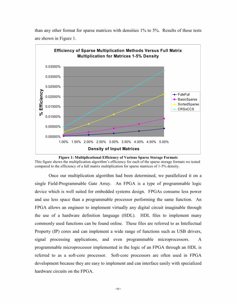
-v-
than any other format for sparse matrices with densities 1% to 5%. Results of these tests
are shown in Figure 1.
Efficiency of Sparse Multiplication Methods Versus Full Matrix
Multiplication for Matrices 1-5% Density
0.00000%
0.00500%
0.01000%
0.01500%
0.02000%
0.02500%
0.03000%
0.03500%
1.00% 1.50% 2.00% 2.50% 3.00% 3.50% 4.00% 4.50% 5.00%
Density of Input Matrices
% Efficiency
FullxFull
BasicSparse
SortedSparse
CRSxCCS
Figure 1: Multiplicational Efficiency of Various Sparse Storage Formats
This figure shows the multiplication algorithm’s efficiency for each of the sparse storage formats we tested
compared to the efficiency of a full matrix multiplication for sparse matrices of 1-5% density.
Once our multiplication algorithm had been determined, we parallelized it on a
single Field-Programmable Gate Array. An FPGA is a type of programmable logic
device which is well suited for embedded systems design. FPGAs consume less power
and use less space than a programmable processor performing the same function. An
FPGA allows an engineer to implement virtually any digital circuit imaginable through
the use of a hardware definition language (HDL). HDL files to implement many
commonly used functions can be found online. These files are referred to as Intellectual
Property (IP) cores and can implement a wide range of functions such as USB drivers,
signal processing applications, and even programmable microprocessors. A
programmable microprocessor implemented in the logic of an FPGA through an HDL is
referred to as a soft-core processor. Soft-core processors are often used in FPGA
development because they are easy to implement and can interface easily with specialized
hardware circuits on the FPGA.
-vi-
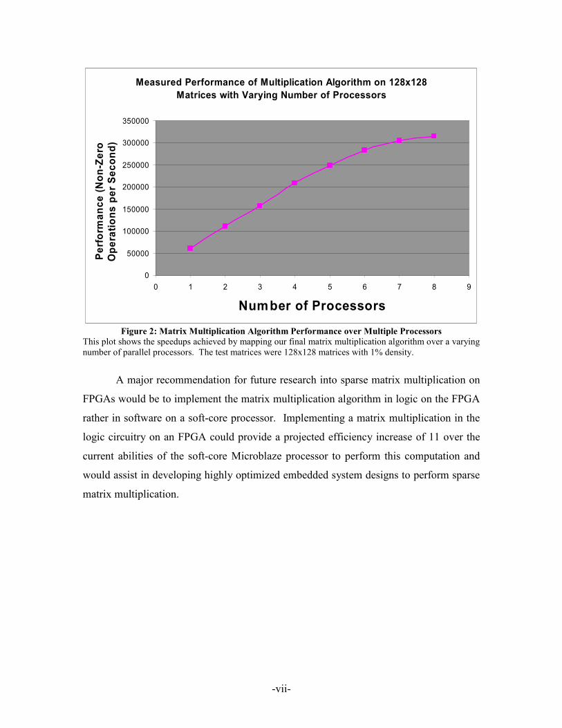
This project used multiple Microblaze soft-core processors working in parallel on
one Xilinx Inc. FPGA to increase the performance of a sparse matrix multiplication
algorithm. Our final design incorporated a highly optimized matrix multiplication
algorithm, a parallel architecture, and an advanced matrix splitting technique to achieve a
parallel speedup of the multiplication algorithm on a single FPGA.
Our final matrix multiplication was able to multiply two sparse matrices, A and B,
stored in CRS and CCS formats, respectively. The algorithm was highly parallelizable
and was capable of computing the product of two 128x128 sparse matrices with 1%
density 49 times faster than the speed at which a full matrix multiplication was capable.
This type of algorithmic performance was comparable to the abilities of other optimized
sparse matrix multiplication algorithms, but was highly parallelizable. A parallel
implementation of this algorithm achieved a speedup of 5.20 when mapped over eight
parallel processors. The algorithm consisted of a load distribution technique that split
matrix B into submatrices of its columns, thereby providing intelligent distribution of the
matrix multiplication workload among multiple processors. Figure 2 shows the measured
speedups provided by parallelizing our algorithm over a varying number of Microblazes.
-vii-
Measured Performance of Multiplication Algorithm on 128x128
Matrices with Varying Number of Processors
0
50000
100000
150000
200000
250000
300000
350000
0 1 2 3 4 5 6 7 8 9
Number of Processors
Performance (Non-Zero
Operations per Second)
Figure 2: Matrix Multiplication Algorithm Performance over Multiple Processors
This plot shows the speedups achieved by mapping our final matrix multiplication algorithm over a varying
number of parallel processors. The test matrices were 128x128 matrices with 1% density.
A major recommendation for future research into sparse matrix multiplication on
FPGAs would be to implement the matrix multiplication algorithm in logic on the FPGA
rather in software on a soft-core processor. Implementing a matrix multiplication in the
logic circuitry on an FPGA could provide a projected efficiency increase of 11 over the
current abilities of the soft-core Microblaze processor to perform this computation and
would assist in developing highly optimized embedded system designs to perform sparse
matrix multiplication.
-viii-
Contributions
This project was completed by Ryan Kendrick and Michael Moukarzel of the
WPI class of 2008.
In the summer of 2007, prior to working on this MQP, Ryan and Michael worked
as summer interns at MIT Lincoln Laboratory. During this period of time, background
research was performed to determine optimized algorithms to be implemented on the
FPGA. Michael focused mostly on the testing and development of various data
structures, multiplication algorithms, and conversions between storage formats while
Ryan focused his efforts on background mathematical research into the algorithms and
the testing of various load distribution techniques.
Once the actual project began Michael shifted his efforts towards the actual
implementation of these algorithms on the Xilinx FPGA in C-code. His work consisted
of the configuring of Microblaze processors and their communication links in hardware
on the FPGA. Also, Michael was responsible for loading code to these Microblazes and
debugging to be sure the code worked properly in the system.
Ryan assisted in technical work for the first few weeks of this project, converting
his MATLAB algorithms for matrix splitting to C-code. After writing this code for the
FPGA implementation, Ryan took on the responsibility of editing the MQP paper.
Though Ryan still took part in every technical decision made during the course of this
project, the primary focus of his efforts was the development of the MQP paper and the
presentations.
Both partners have reviewed their contributions to this project and both feel that
each contributed equally to the overall efforts involved in completing this project.
-ix-
Table of Contents
Abstract ............................................................................................................................... ii
Executive Summary........................................................................................................... iii
Contributions.................................................................................................................... viii
List of Illustrations............................................................................................................. xi
1 Introduction............................................................................................................... 13
1.1 Project Goals..................................................................................................... 17
1.1.1 Goal Measurementt Metrics...................................................................... 18
2 Background ............................................................................................................... 19
2.1 Graph Processing .............................................................................................. 19
2.2 Sparse Matrices................................................................................................. 22
2.2.1 Sparse Matrix Storage............................................................................... 23
2.2.2 Compressed Column Storage (CCS) ........................................................ 24
2.2.3 Compressed Row Storage (CRS).............................................................. 26
2.2.4 The Length Vector vs. Pointer .................................................................. 26
2.2.5 Compressed Diagonal Storage (CDS) ...................................................... 27
2.2.6 Storage Size Comparison.......................................................................... 30
2.2.7 Matrix Multiplication................................................................................ 32
2.3 Matrices of Interest ........................................................................................... 33
2.4 Field Programmable Gate Arrays (FPGAs)...................................................... 36
2.4.1 FPGA Architecture ................................................................................... 38
2.4.2 Soft-Core Microprocessors ....................................................................... 41
2.4.3 PowerPC processor ................................................................................... 44
2.5 ML310 Development Board ............................................................................. 45
2.6 Xilinx Virtex-II Pro XC2VP30......................................................................... 48
3 Algorithm Performance Analysis ............................................................................. 49
3.1 Optimized Matrix Multiplication Algorithm .................................................... 49
3.1.1 Full Matrix Multiplication ........................................................................ 51
3.1.2 Sparse Matrix Multiplication .................................................................... 52
3.1.3 Sorted Sparse Matrix Multiplication......................................................... 53
3.1.4 CRS x CCS Matrix Multiplication Using Pointer .................................... 55
3.1.5 CRS x CCS Matrix Multiplication Using Length..................................... 56
3.1.6 Counting Non-Zero Operations ................................................................ 56
3.1.7 Algorithm Efficiency Results ................................................................... 57
3.2 Optimized Parallelization and Load Balancing Technique .............................. 59
3.2.1 Pointer vs. Length Vector in Parallelization ............................................. 61
3.2.2 Block-Column Distribution ...................................................................... 64
3.2.3 Block-Values Distribution ........................................................................ 65
3.2.4 Block-Cyclic Distribution......................................................................... 67
3.2.5 Inverse Block-Cyclic Distribution ............................................................ 68
3.2.6 Column-Cyclic Distribution...................................................................... 69
3.2.7 Performance Evaluation of Load Balancing Techniques.......................... 70
4 FPGA Implementation .............................................................................................. 75
-x-
4.1.1 Microblaze Multiplication ........................................................................ 75
4.1.2 Parallel Microblaze Load Distribution...................................................... 76
5 Algorithm Performance Results................................................................................ 78
5.1 CRSxCCS Multiplication vs. Full Matrix Multiplication in C ......................... 79
5.2 Theoretical Maximum Allowable Matrix Size ................................................. 80
5.3 FPGA Parallel Speedup Predictions ................................................................. 86
5.3.1 Microblaze Execution Speed .................................................................... 86
5.3.2 Fast Simplex Link ..................................................................................... 88
5.3.3 Microblaze System Theoretical Performance Estimate............................ 89
5.4 FPGA Parallel Speedup Measurements ............................................................ 90
6 Discussion and Conclusions ..................................................................................... 95
6.1 Sparse Matrix Multiplication Algorithm .......................................................... 95
6.2 Parallelization of Multiplication Algorithm on FPGA ..................................... 96
6.3 Future Recommendations ................................................................................. 97
6.4 Future Impacts ................................................................................................ 100
Annotated Reference List ............................................................................................... 103
Appendix A..................................................................................................................... 108
Full Matrix Multiplication .......................................................................................... 108
Basic Sparse Matrix Multiplication (Unsorted).......................................................... 108
Sorted Sparse Matrix Multiplication........................................................................... 110
Compressed Sparse Matrix Multiplication (CRSxCCS) using Pointer Vector ......... 111
Compressed Sparse Matrix Multiplication (CRSxCCS) using Length vector............ 112
Appendix B ..................................................................................................................... 114
Block-Column Distribution ........................................................................................ 114
Block-Values Distribution .......................................................................................... 115
Block-Cyclic Distribution........................................................................................... 117
Inverse Block-Cyclic Distribution .............................................................................. 120
Column-Cyclic Distribution........................................................................................ 123
Appendix C ..................................................................................................................... 125
Appendix D..................................................................................................................... 127
Appendix E ..................................................................................................................... 128
Column-Cyclic Splitting ............................................................................................. 128
Column-Cyclic Reassembly........................................................................................ 129
Appendix F...................................................................................................................... 131
Appendix G..................................................................................................................... 142
Appendix H..................................................................................................................... 143
Appendix I ...................................................................................................................... 149
Appendix J ...................................................................................................................... 151
IEEE Code of Ethics ....................................................................................................... 153
-xi-
List of Illustrations
Figure 1: Multiplicational Efficiency of Various Sparse Storage Formats......................... v
Figure 2: Matrix Multiplication Algorithm Performance over Multiple Processors ........ vii
Figure 3: Graph Example.................................................................................................. 13
Figure 4: Knowledge Processing ...................................................................................... 15
Figure 5: Small Social Network Represented by a Graph ................................................ 19
Figure 6: Adjacency Matrix Representation of Social Network Graph............................ 20
Figure 7: Full Matrix Format ............................................................................................ 23
Figure 8: Sparse Matrix Format........................................................................................ 24
Figure 9: Compressed Column Format (CCS).................................................................. 25
Figure 10: Compressed Row Format (CRS)..................................................................... 26
Figure 11: Compressed Column using Length Vector ..................................................... 27
Figure 12: Diagonal Assignments in Compressed Diagonal Storage............................... 28
Figure 13: Diagonal Vector Example ............................................................................... 28
Figure 14: Diagonal Values .............................................................................................. 29
Figure 15: Banded Matrix Example.................................................................................. 30
Figure 16: Storage Method Sizes on a Square Matrix ...................................................... 31
Figure 17: General form for Matrix Multiplication .......................................................... 32
Figure 18: General Form for Computing a Dot Product................................................... 33
Figure 19: Structured RMAT Matrix................................................................................ 34
Figure 20: Randomized RMAT Matrix ............................................................................ 35
Figure 21: Performance Density and Efficiency between device families ....................... 37
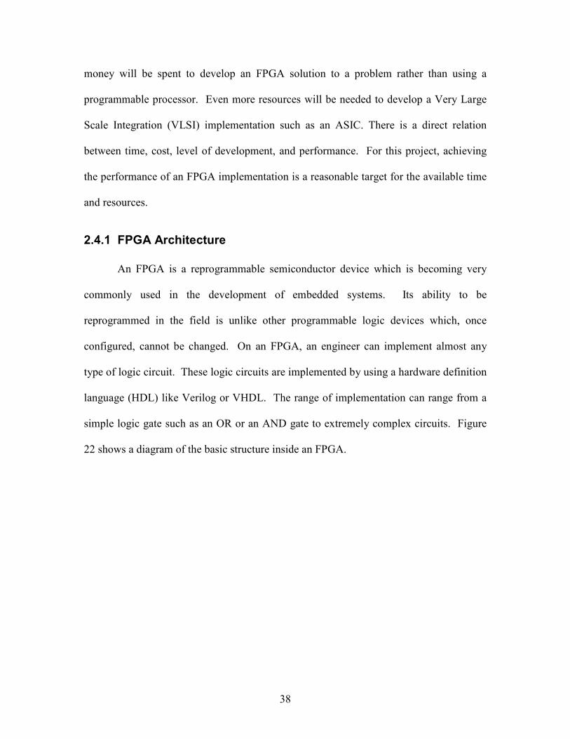
Figure 22: FPGA Architecture.......................................................................................... 39
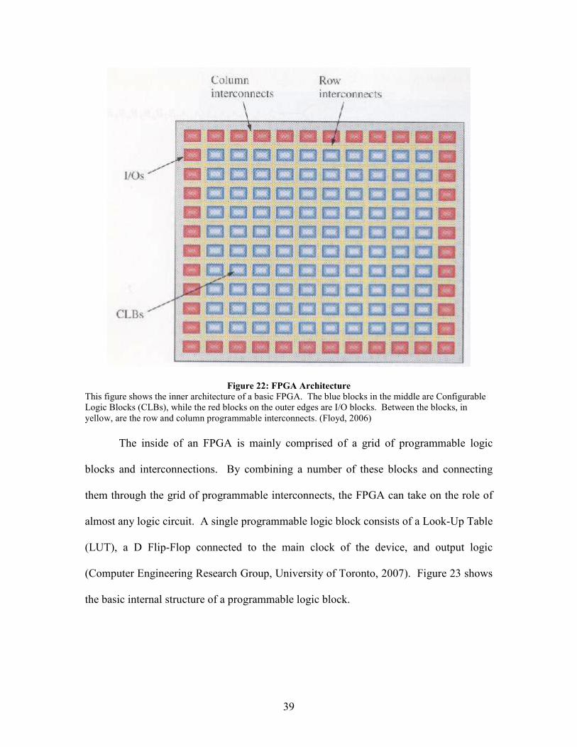
Figure 23: FPGA Logic Block.......................................................................................... 40
Figure 24: Microblaze Architecture.................................................................................. 43
Figure 25: Software Algorithm vs. Hardware................................................................... 44
Figure 26: PowerPC Architecture..................................................................................... 45
Figure 27: Xilinx ML310 Development Board ................................................................ 47
Figure 28: Data Locality in Sorted Sparse Matrix Multiplication .................................... 54
Figure 29: Efficiency of Different Multiplication Methods 1-99% Density .................... 57
Figure 30: Efficiency of Different Multiplication Methods 1-5% Density ...................... 58
Figure 31: Parallelization Block Diagram ........................................................................ 60
Figure 32: Splitting a Full Matrix into Smaller Matrices ................................................. 62
Figure 33: Split Matrices Stored using Pointer................................................................. 62
Figure 34: Split Matrices Stored using Length ................................................................. 63
Figure 35: Block-Column Load Distribution.................................................................... 65
Figure 36: Block-Values Load Distribution ..................................................................... 66
Figure 37: Block-Cyclic Load Distribution ...................................................................... 68
Figure 38: Inverse Block-Cyclic Load Distribution ......................................................... 69
Figure 39: Performance of Various Load Balancing Techniques on Structured Matrix .. 72
Figure 40: Performance of Various Load Balancing Techniques on Randomized Matrix74
Figure 41: Allowable Memory per Input Matrix Estimate ............................................... 82
Figure 42: Required Memory Space of Compressed Matrix ............................................ 84
Figure 43: Size of Input Matrices vs Number of Processors ............................................ 85
Figure 44: Theoretical Parallel Microblaze Performance................................................. 89
-xii-
Figure 45: Parallel System of Microblazes....................................................................... 91
Figure 46: Measured Performance of Parallel Multiplication of 128x128 Matrices ........ 93
Figure 47: Realistic Timeline of Parallel Algorithm ........................................................ 94
Figure 48: Proposed Logic Circuit States to Perform Matrix Multiplication ................... 99
Figure 49: Projected Speedups with Microblazes and Logic Circuits ............................ 100
Figure 50: Parallelizable Algorithm in Multiple Computer Environments .................... 102
13
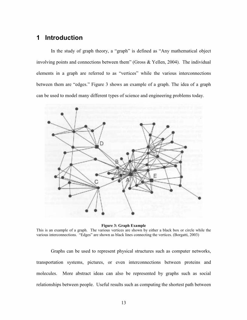
1 Introduction
In the study of graph theory, a “graph” is defined as “Any mathematical object
involving points and connections between them” (Gross & Yellen, 2004). The individual
elements in a graph are referred to as “vertices” while the various interconnections
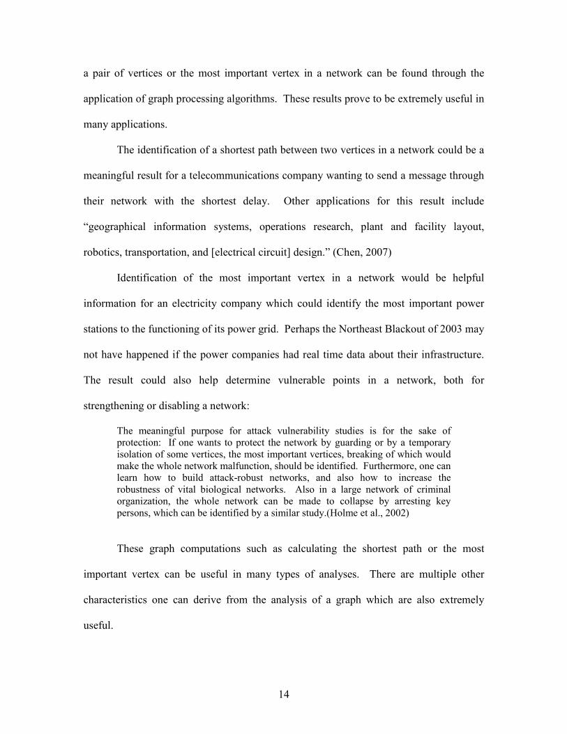
between them are “edges.” Figure 3 shows an example of a graph. The idea of a graph
can be used to model many different types of science and engineering problems today.
Figure 3: Graph Example
This is an example of a graph. The various vertices are shown by either a black box or circle while the
various interconnections. “Edges” are shown as black lines connecting the vertices. (Borgatti, 2003)
Graphs can be used to represent physical structures such as computer networks,
transportation systems, pictures, or even interconnections between proteins and
molecules. More abstract ideas can also be represented by graphs such as social
relationships between people. Useful results such as computing the shortest path between
14
a pair of vertices or the most important vertex in a network can be found through the
application of graph processing algorithms. These results prove to be extremely useful in
many applications.
The identification of a shortest path between two vertices in a network could be a
meaningful result for a telecommunications company wanting to send a message through
their network with the shortest delay. Other applications for this result include
“geographical information systems, operations research, plant and facility layout,
robotics, transportation, and [electrical circuit] design.” (Chen, 2007)
Identification of the most important vertex in a network would be helpful
information for an electricity company which could identify the most important power
stations to the functioning of its power grid. Perhaps the Northeast Blackout of 2003 may
not have happened if the power companies had real time data about their infrastructure.
The result could also help determine vulnerable points in a network, both for
strengthening or disabling a network:
The meaningful purpose for attack vulnerability studies is for the sake of
protection: If one wants to protect the network by guarding or by a temporary
isolation of some vertices, the most important vertices, breaking of which would
make the whole network malfunction, should be identified. Furthermore, one can
learn how to build attack-robust networks, and also how to increase the
robustness of vital biological networks. Also in a large network of criminal
organization, the whole network can be made to collapse by arresting key
persons, which can be identified by a similar study.(Holme et al., 2002)
These graph computations such as calculating the shortest path or the most
important vertex can be useful in many types of analyses. There are multiple other
characteristics one can derive from the analysis of a graph which are also extremely
useful.
15
At MIT Lincoln Laboratory in Lexington, Massachusetts researchers work on the
development of highly sophisticated surveillance and intelligence systems. Group 102,
the Embedded Digital Systems group, focuses on what is called knowledge processing.
Knowledge processing is the act by which raw data from a camera, radar, antenna, or
some other sensor, is converted into useable information. In these surveillance systems,
this work is carried out by small embedded computer systems which accompany the
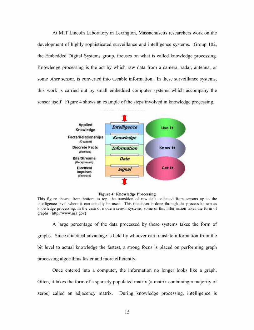
sensor itself. Figure 4 shows an example of the steps involved in knowledge processing.
Figure 4: Knowledge Processing
This figure shows, from bottom to top, the transition of raw data collected from sensors up to the
intelligence level where it can actually be used. This transition is done through the process known as
knowledge processing. In the case of modern sensor systems, some of this information takes the form of
graphs. (http://www.nsa.gov)
A large percentage of the data processed by these systems takes the form of
graphs. Since a tactical advantage is held by whoever can translate information from the
bit level to actual knowledge the fastest, a strong focus is placed on performing graph
processing algorithms faster and more efficiently.
Once entered into a computer, the information no longer looks like a graph.
Often, it takes the form of a sparsely populated matrix (a matrix containing a majority of
zeros) called an adjacency matrix. During knowledge processing, intelligence is
16
extracted from the matrices using various algorithmic tools. A common kernel
performed in these algorithms is the multiplication of two adjacency matrices. Tests on
matrix multiplication algorithm performance have been conducted by group 102 of MIT
Lincoln Laboratory. The results showed efficiencies, or the percentage of arithmetic
operations performed out of the peak possible arithmetic operations, of between 0.05 and
0.1% when performed on conventional microprocessor systems (Bliss, 2007).
Our project focused on finding a matrix multiplication algorithm that performed
with efficiency similar to those of current algorithms, but was highly parallelizable. We
focused on demonstrating the parallelizable properties of our algorithm through
implementation on a system of multiple parallel processors in an embedded system
design. This design achieved speedup through the utilization of the matrix multiplication
algorithm and a load distribution algorithm which distributed the workload evenly among
parallel processors.
Since certain advantages can be had when dealing with a sparse matrix, this
project explored various formats for the storage of sparse matrices. These formats were
used to develop a more efficient algorithm for the multiplication of sparse matrices.
Once an optimized matrix multiplication algorithm was developed, an effective method
for parallelizing its operations on an embedded system was determined.
The final result of this project was to implement a field-programmable gate array
(FPGA), a common type of programmable logic chip in embedded system design, which
was capable of performing our algorithm. The FPGA implementation demonstrated how
the matrix multiplication process, a key kernel in graph processing, can be made more
17
efficient by exploiting the sparsity of the matrices in a more efficient multiplication
algorithm and how parallelization of operations can speed up the entire kernel.
The two main goals of this project were to develop an efficient algorithm for the
multiplication of two sparse matrices and to implement a way of easily parallelizing this
algorithm in a small embedded system. By utilizing a sparse matrix storage method, the
storage requirements for many matrices that, if stored in full format, were too large to be
stored on an FPGA, became small enough be processed in a single FPGA. With multiple
processors working together in parallel, the final FPGA design performed perform many
more non-zero arithmetic operations per second than a single processor could perform.
The final result design can serve as an example for future research into the area of
optimized sparse matrix multiplication. It can also serve as a model for a complete
hardware implementation of this algorithm, such as the development of an Application-
Specific Integrated Circuit (ASIC) which would be able to perform these multiplications
faster than any other device.
1.1 Project Goals
The goals of this project were as follows:
1. To determine a highly parallelizable method for the storage and multiplication of two
sparsely populated matrices which can perform computations at efficiencies comparable
to the 0.05% to 0.1% achieved by optimized sparse matrix multiplications on traditional
microprocessor systems
2. To demonstrate how the optimized multiplication algorithm can be parallelized on a
single FPGA to achieve a parallel speedup by distributing the load over multiple
processing elements.
18
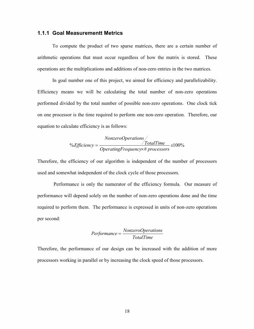
1.1.1 Goal Measurementt Metrics
To compute the product of two sparse matrices, there are a certain number of
arithmetic operations that must occur regardless of how the matrix is stored. These
operations are the multiplications and additions of non-zero entries in the two matrices.
In goal number one of this project, we aimed for efficiency and parallelizability.
Efficiency means we will be calculating the total number of non-zero operations
performed divided by the total number of possible non-zero operations. One clock tick
on one processor is the time required to perform one non-zero operation. Therefore, our
equation to calculate efficiency is as follows:
%100#
% xprocessorsrequencyOperatingF
TotalTimerationsNonzeroOpe
Efficiency×
=
Therefore, the efficiency of our algorithm is independent of the number of processors
used and somewhat independent of the clock cycle of those processors.
Performance is only the numerator of the efficiency formula. Our measure of
performance will depend solely on the number of non-zero operations done and the time
required to perform them. The performance is expressed in units of non-zero operations
per second:
TotalTime
rationsNonzeroOpeePerformanc =
Therefore, the performance of our design can be increased with the addition of more
processors working in parallel or by increasing the clock speed of those processors.
19
2 Background
2.1 Graph Processing
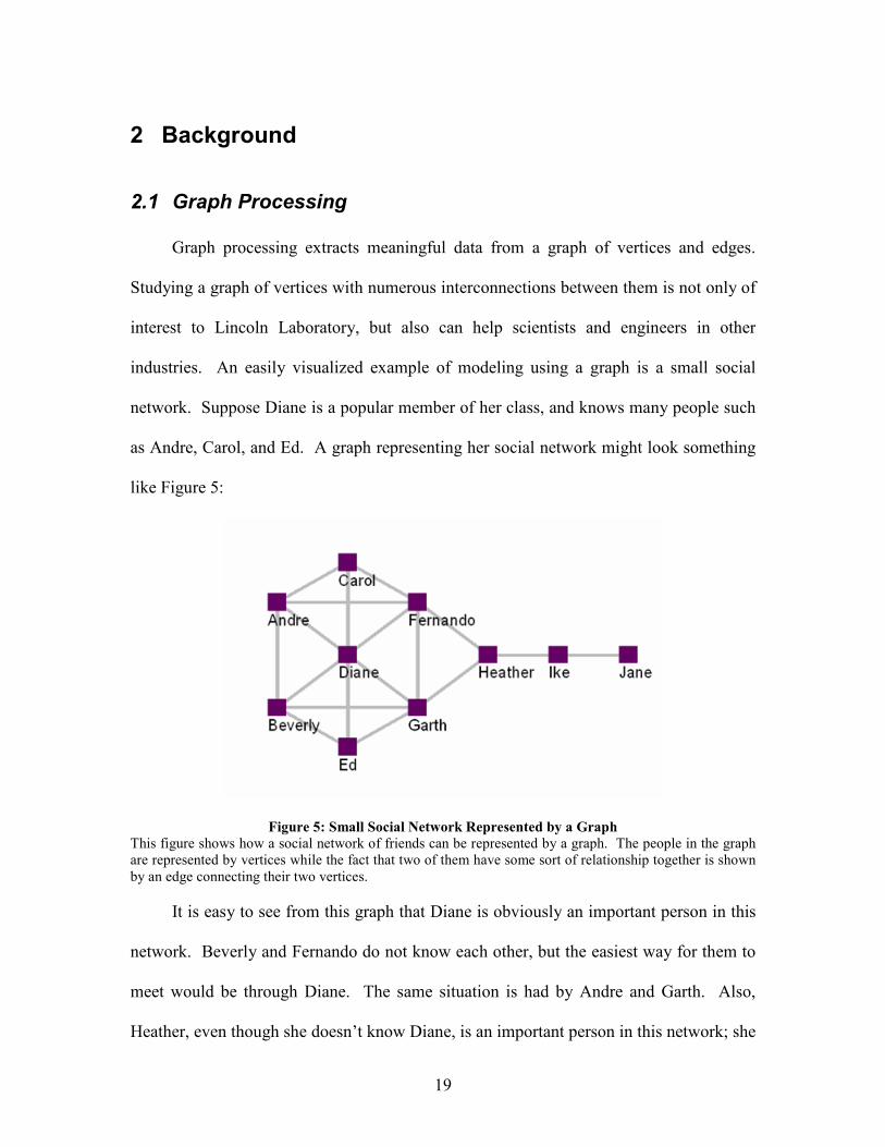
Graph processing extracts meaningful data from a graph of vertices and edges.
Studying a graph of vertices with numerous interconnections between them is not only of
interest to Lincoln Laboratory, but also can help scientists and engineers in other
industries. An easily visualized example of modeling using a graph is a small social
network. Suppose Diane is a popular member of her class, and knows many people such
as Andre, Carol, and Ed. A graph representing her social network might look something
like Figure 5:
Figure 5: Small Social Network Represented by a Graph
This figure shows how a social network of friends can be represented by a graph. The people in the graph
are represented by vertices while the fact that two of them have some sort of relationship together is shown
by an edge connecting their two vertices.
It is easy to see from this graph that Diane is obviously an important person in this
network. Beverly and Fernando do not know each other, but the easiest way for them to
meet would be through Diane. The same situation is had by Andre and Garth. Also,
Heather, even though she doesn’t know Diane, is an important person in this network; she
20
serves as the only connection between Ike and Jane and the rest of the network.
(Robinson, 2007)
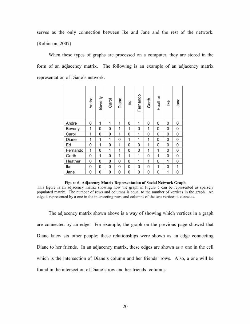
When these types of graphs are processed on a computer, they are stored in the
form of an adjacency matrix. The following is an example of an adjacency matrix
representation of Diane’s network.
Andre
Beverly
Carol
Diane
Ed
Fernando
Garth
Heather
Ike
Jane
Andre 0 1 1 1 0 1 0 0 0 0
Beverly 1 0 0 1 1 0 1 0 0 0
Carol 1 0 0 1 0 1 0 0 0 0
Diane 1 1 1 0 1 1 1 0 0 0
Ed 0 1 0 1 0 0 1 0 0 0
Fernando 1 0 1 1 0 0 1 1 0 0
Garth 0 1 0 1 1 1 0 1 0 0
Heather 0 0 0 0 0 1 1 0 1 0
Ike 0 0 0 0 0 0 0 1 0 1
Jane 0 0 0 0 0 0 0 0 1 0
Figure 6: Adjacency Matrix Representation of Social Network Graph
This figure is an adjacency matrix showing how the graph in Figure 5 can be represented as sparsely
populated matrix. The number of rows and columns is equal to the number of vertices in the graph. An
edge is represented by a one in the intersecting rows and columns of the two vertices it connects.
The adjacency matrix shown above is a way of showing which vertices in a graph
are connected by an edge. For example, the graph on the previous page showed that
Diane knew six other people; these relationships were shown as an edge connecting
Diane to her friends. In an adjacency matrix, these edges are shown as a one in the cell
which is the intersection of Diane’s column and her friends’ rows. Also, a one will be
found in the intersection of Diane’s row and her friends’ columns.
21
Zeros are found along the main diagonal, in the intersection of each person’s row
and column. Some adjacency matrices store all ones along the main diagonal and some
do not; whether these cells are filled with zeros or not usually depends on the application.
Also, while the adjacency matrix in Figure 6 has symmetry across the diagonal, not all
adjacency matrices have this symmetry. In unidirectional adjacency matrices, vertex A
can be connected to vertex B without B being connected back to A.
Adjacency matrices sometimes use values other than one in cells to show the
strength of an edge. For example, if Andre and Fernando were brothers rather than just
friends, a three or a four may be contained in their intersecting cells rather than just a one
to signify a stronger relationship.
Once these graphs grow to contain hundreds or thousands of vertices and edges,
computers become responsible for locating the important vertices. To find them, an
algorithm to find the “betweenness centrality” of a certain vertex is used. Vertices which
are on the shortest path between many other pairs of vertices have a high betweenness
centrality. In the graph example, Diane appeared on the shortest path between many
other people, therefore she was an important vertex on the graph.
The matrix representation of a graph is commonly large and sparsely populated. In
the adjacency matrix above, there are 100 cells, only 36 of which contain a non-zero
value; commonly, this type of matrix is referred to as a sparse matrix. For a graph with N
vertices, the number of cells in its adjacency matrix is N2. When dealing with a graph of
tens or even hundreds of thousands of vertices, adjacency matrices become too large to
be processed by an average desktop computer.
22
Though betweenness centrality algorithms are complicated and outside the scope of
this project, their performance “is dominated by sparse matrix multiply performance”
(Robinson, 2007). The sparse matrix multiply kernel is the limiting factor in performing
this algorithm. Conventional algorithms which perform these multiplications prove
extremely inefficient. Since the number of zeros in a sparse matrix is high, the frequency
of a meaningful calculation—multiplying or adding two non-zero values together—is
low. Often, when sparse matrix multiplication algorithms are performed on a
conventional processor, the frequency of non-zero multiplies with relation to the
computer’s clock cycle is low, between 0.05% and 0.1%. To effectively handle sparse
matrices, specialized formats can be used to store only the non-zero values, thus
shrinking the size of the matrix in memory greatly. These formats will be discussed in
the next section.
2.2 Sparse Matrices
There is no concrete rule defining when a matrix is sparse and when it is not.
Professor Tim Davis from the University of Florida claims a sparse matrix is: “…any
matrix with enough zeros that it pays to take advantage of them” (Davis, 2007). This
definition means that whether or not a matrix is sparse depends on how many zero entries
it has as well as how well the user can take advantage of those zeros. When dealing with
large sparsely populated matrices, an increasingly common technique to process and store
them is to take advantage of their sparsity. Since many of the sparse matrices used in
science and engineering today have large dimensions, on the order of tens or hundreds of
thousands, exploiting the sparsity of a matrix can give enormous advantages in both
storage space required and processing efficiency. There are two ways one would exploit
23
the sparsity of a matrix: first, to store only the non-zero elements of the matrix and
second, to process only the non-zero elements of the matrix. (Zlatev, 1991)
2.2.1 Sparse Matrix Storage
A full matrix representation of a matrix stores every value, regardless of whether
it is zero or non-zero. The total size is approximately equal to:
)(#)(# ofColumnsofRowsMemoryFullMatrix ×=
Note: This calculation is approximate because some other small values may be
stored such as the number of rows and the number of columns. If this matrix is sparsely
populated, meaning it contains a majority of zero entries, the storage space can be
reduced greatly by using a sparse matrix storage technique. To demonstrate how one
converts a sparsely populated matrix into a sparse matrix format an example will be
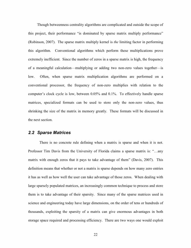
given. Figure 7 is a five by five full matrix with only eight non-zero entries: Only eight
non-zeros means the computer is storing 17 zero values which are not needed.
Figure 7: Full Matrix Format
The full matrix storage format is shown above. It stores all values in the matrix, non-zero and zero. It
becomes an inefficient storage method when the majority of the values are zero.
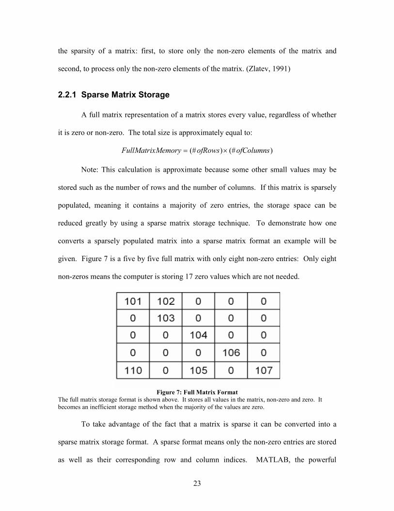
To take advantage of the fact that a matrix is sparse it can be converted into a
sparse matrix storage format. A sparse format means only the non-zero entries are stored
as well as their corresponding row and column indices. MATLAB, the powerful
24
mathematics and engineering program, currently uses this basic sparse matrix format.
The following figure is the same matrix as shown above stored in the basic sparse format.
Figure 8: Sparse Matrix Format
The most basic form of sparse matrix storage formats. It stores the corresponding row, column, and value
of every non-zero entry in the matrix.
The total space required to store a matrix in the basic sparse matrix format is
approximately equal to:
)(#3 NonzerosoryeMatrixMemBasicSpars ×=
This method stores three values for every non-zero entry in the matrix. Therefore, for
matrices with less than 33% density, the sparse matrix storage method will use less
memory space than a full matrix storage method.
2.2.2 Compressed Column Storage (CCS)
The fact that the column vector is sorted can be taken advantage of to further
compress this matrix. Instead of storing the column vector entirely, a column pointer can
be stored. The column pointer is a vector telling the user when the column pointer
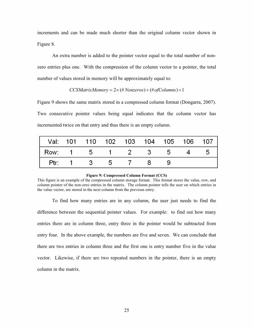
25
increments and can be made much shorter than the original column vector shown in
Figure 8.
An extra number is added to the pointer vector equal to the total number of non-
zero entries plus one. With the compression of the column vector to a pointer, the total
number of values stored in memory will be approximately equal to:
1)(#)(#2 ++×= ofColumnsNonzerosemoryCCSMatrixM
Figure 9 shows the same matrix stored in a compressed column format (Dongarra, 2007).
Two consecutive pointer values being equal indicates that the column vector has
incremented twice on that entry and thus there is an empty column.
Figure 9: Compressed Column Format (CCS)
This figure is an example of the compressed column storage format. This format stores the value, row, and
column pointer of the non-zero entries in the matrix. The column pointer tells the user on which entries in
the value vector, are stored in the next column from the previous entry.
To find how many entries are in any column, the user just needs to find the
difference between the sequential pointer values. For example: to find out how many
entries there are in column three, entry three in the pointer would be subtracted from
entry four. In the above example, the numbers are five and seven. We can conclude that
there are two entries in column three and the first one is entry number five in the value
vector. Likewise, if there are two repeated numbers in the pointer, there is an empty
column in the matrix.
26
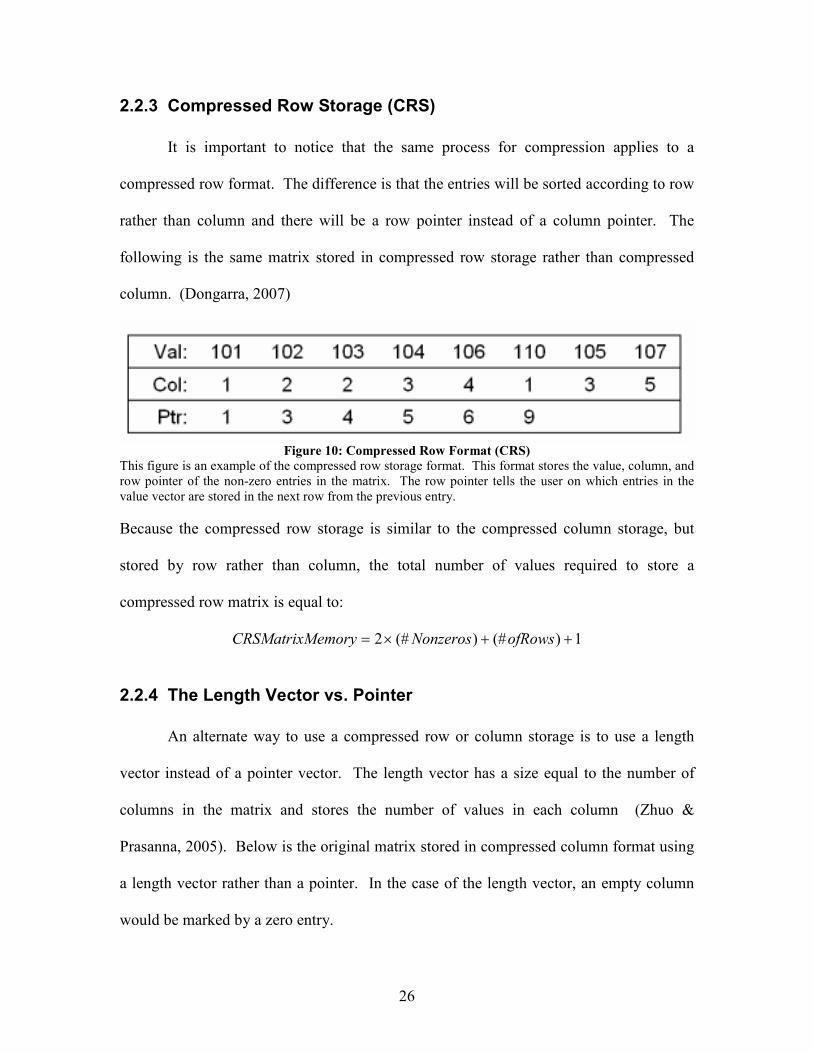
2.2.3 Compressed Row Storage (CRS)
It is important to notice that the same process for compression applies to a
compressed row format. The difference is that the entries will be sorted according to row
rather than column and there will be a row pointer instead of a column pointer. The
following is the same matrix stored in compressed row storage rather than compressed
column. (Dongarra, 2007)
Figure 10: Compressed Row Format (CRS)
This figure is an example of the compressed row storage format. This format stores the value, column, and
row pointer of the non-zero entries in the matrix. The row pointer tells the user on which entries in the
value vector are stored in the next row from the previous entry.
Because the compressed row storage is similar to the compressed column storage, but
stored by row rather than column, the total number of values required to store a
compressed row matrix is equal to:
1)(#)(#2 ++×= ofRowsNonzerosemoryCRSMatrixM
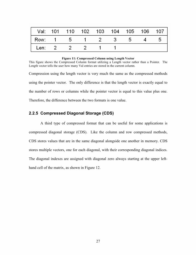
2.2.4 The Length Vector vs. Pointer
An alternate way to use a compressed row or column storage is to use a length
vector instead of a pointer vector. The length vector has a size equal to the number of
columns in the matrix and stores the number of values in each column (Zhuo &
Prasanna, 2005). Below is the original matrix stored in compressed column format using
a length vector rather than a pointer. In the case of the length vector, an empty column
would be marked by a zero entry.
27
Figure 11: Compressed Column using Length Vector
This figure shows the Compressed Column format utilizing a Length vector rather than a Pointer. The
Length vector tells the user how many Val entries are stored in the current column.
Compression using the length vector is very much the same as the compressed methods
using the pointer vector. The only difference is that the length vector is exactly equal to
the number of rows or columns while the pointer vector is equal to this value plus one.
Therefore, the difference between the two formats is one value.
2.2.5 Compressed Diagonal Storage (CDS)
A third type of compressed format that can be useful for some applications is
compressed diagonal storage (CDS). Like the column and row compressed methods,
CDS stores values that are in the same diagonal alongside one another in memory. CDS
stores multiple vectors, one for each diagonal, with their corresponding diagonal indices.
The diagonal indexes are assigned with diagonal zero always starting at the upper left-
hand cell of the matrix, as shown in Figure 12.
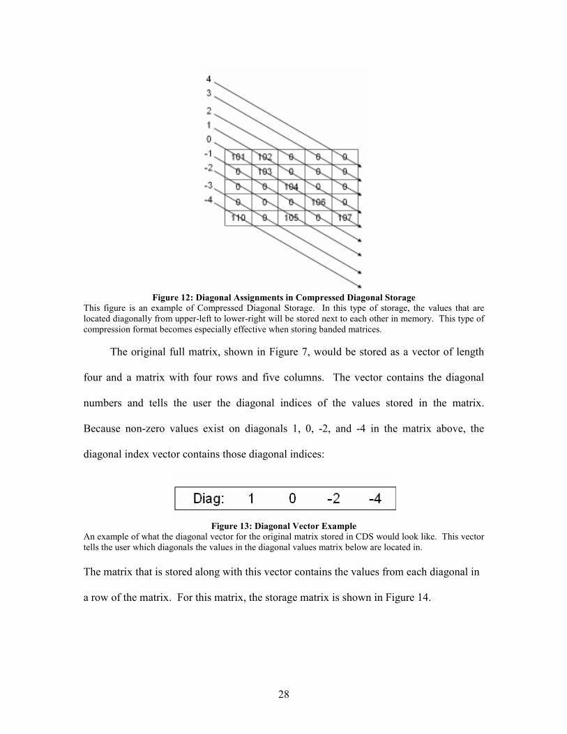
28
Figure 12: Diagonal Assignments in Compressed Diagonal Storage
This figure is an example of Compressed Diagonal Storage. In this type of storage, the values that are
located diagonally from upper-left to lower-right will be stored next to each other in memory. This type of
compression format becomes especially effective when storing banded matrices.
The original full matrix, shown in Figure 7, would be stored as a vector of length
four and a matrix with four rows and five columns. The vector contains the diagonal
numbers and tells the user the diagonal indices of the values stored in the matrix.
Because non-zero values exist on diagonals 1, 0, -2, and -4 in the matrix above, the
diagonal index vector contains those diagonal indices:
Figure 13: Diagonal Vector Example
An example of what the diagonal vector for the original matrix stored in CDS would look like. This vector
tells the user which diagonals the values in the diagonal values matrix below are located in.
The matrix that is stored along with this vector contains the values from each diagonal in
a row of the matrix. For this matrix, the storage matrix is shown in Figure 14.
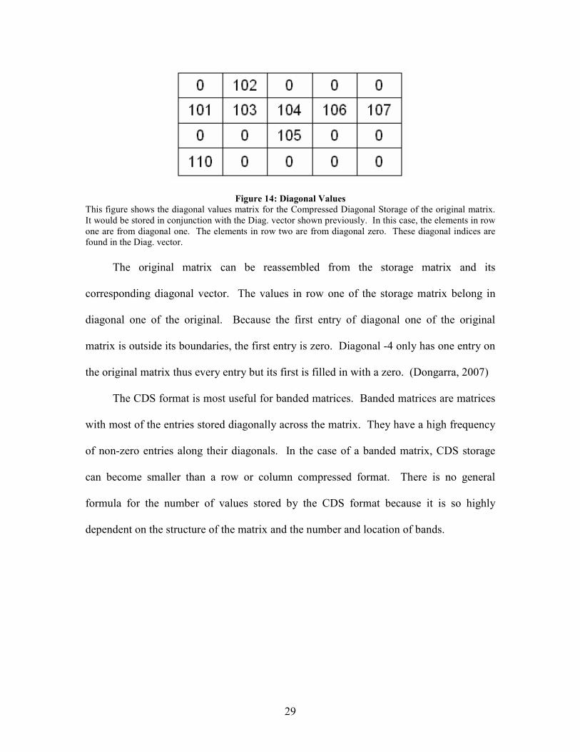
29
Figure 14: Diagonal Values
This figure shows the diagonal values matrix for the Compressed Diagonal Storage of the original matrix.
It would be stored in conjunction with the Diag. vector shown previously. In this case, the elements in row
one are from diagonal one. The elements in row two are from diagonal zero. These diagonal indices are
found in the Diag. vector.
The original matrix can be reassembled from the storage matrix and its
corresponding diagonal vector. The values in row one of the storage matrix belong in
diagonal one of the original. Because the first entry of diagonal one of the original
matrix is outside its boundaries, the first entry is zero. Diagonal -4 only has one entry on
the original matrix thus every entry but its first is filled in with a zero. (Dongarra, 2007)
The CDS format is most useful for banded matrices. Banded matrices are matrices
with most of the entries stored diagonally across the matrix. They have a high frequency
of non-zero entries along their diagonals. In the case of a banded matrix, CDS storage
can become smaller than a row or column compressed format. There is no general
formula for the number of values stored by the CDS format because it is so highly
dependent on the structure of the matrix and the number and location of bands.
30
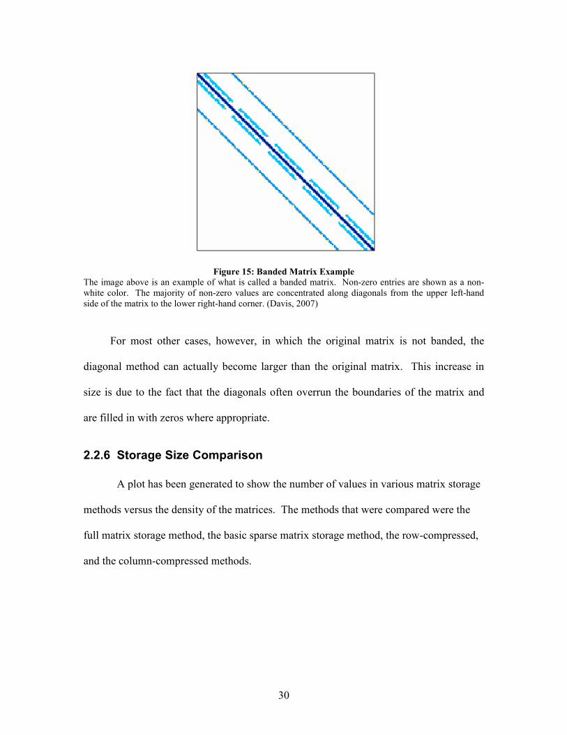
Figure 15: Banded Matrix Example
The image above is an example of what is called a banded matrix. Non-zero entries are shown as a non-
white color. The majority of non-zero values are concentrated along diagonals from the upper left-hand
side of the matrix to the lower right-hand corner. (Davis, 2007)
For most other cases, however, in which the original matrix is not banded, the
diagonal method can actually become larger than the original matrix. This increase in
size is due to the fact that the diagonals often overrun the boundaries of the matrix and
are filled in with zeros where appropriate.
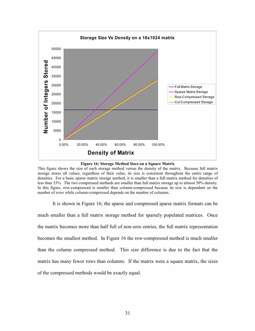
2.2.6 Storage Size Comparison
A plot has been generated to show the number of values in various matrix storage
methods versus the density of the matrices. The methods that were compared were the
full matrix storage method, the basic sparse matrix storage method, the row-compressed,
and the column-compressed methods.
31
Storage Size Vs Density on a 16x1024 matrix
0
5000
10000
15000
20000
25000
30000
35000
40000
45000
50000
0.00% 20.00% 40.00% 60.00% 80.00% 100.00%
Density of Matrix
Number of Integers Stored
Full Matrix Storage
Sparse Matrix Storage
Row-Compressed Storage
Col-Compressed Storage
Figure 16: Storage Method Sizes on a Square Matrix
This figure shows the size of each storage method versus the density of the matrix. Because full matrix
storage stores all values, regardless of their value, its size is consistent throughout the entire range of
densities. For a basic sparse matrix storage method, it is smaller than a full matrix method for densities of
less than 33%. The two compressed methods are smaller than full matrix storage up to almost 50% density.
In this figure, row-compressed is smaller than column-compressed because its size is dependant on the
number of rows while column-compressed depends on the number of columns.
It is shown in Figure 16; the sparse and compressed sparse matrix formats can be
much smaller than a full matrix storage method for sparsely populated matrices. Once
the matrix becomes more than half full of non-zero entries, the full matrix representation
becomes the smallest method. In Figure 16 the row-compressed method is much smaller
than the column compressed method. This size difference is due to the fact that the
matrix has many fewer rows than columns. If the matrix were a square matrix, the sizes
of the compressed methods would be exactly equal.
32
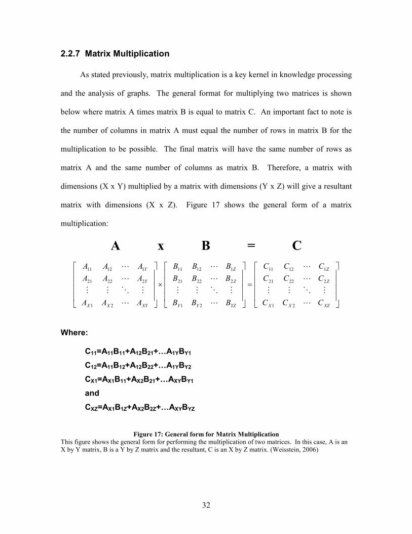
2.2.7 Matrix Multiplication
As stated previously, matrix multiplication is a key kernel in knowledge processing
and the analysis of graphs. The general format for multiplying two matrices is shown
below where matrix A times matrix B is equal to matrix C. An important fact to note is
the number of columns in matrix A must equal the number of rows in matrix B for the
multiplication to be possible. The final matrix will have the same number of rows as
matrix A and the same number of columns as matrix B. Therefore, a matrix with
dimensions (X x Y) multiplied by a matrix with dimensions (Y x Z) will give a resultant
matrix with dimensions (X x Z). Figure 17 shows the general form of a matrix
multiplication:
A x B = C
=
×
XZXX
Z
Z
YZYY
Z
Z
XYXX
Y
Y
CCC
CCC
CCC
BBB
BBB
BBB
AAA
AAA
AAA
L
MOMM
L
L
L
MOMM
L
L
L
MOMM
L
L
21
22221
11211
21
22221
11211
21
22221
11211
Where: C11=A11B11+A12B21+…A1YBY1
C12=A11B12+A12B22+…A1YBY2
CX1=AX1B11+AX2B21+…AXYBY1
and
CXZ=AX1B1Z+AX2B2Z+…AXYBYZ
Figure 17: General form for Matrix Multiplication
This figure shows the general form for performing the multiplication of two matrices. In this case, A is an
X by Y matrix, B is a Y by Z matrix and the resultant, C is an X by Z matrix. (Weisstein, 2006)
33
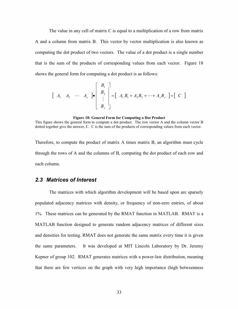
The value in any cell of matrix C is equal to a multiplication of a row from matrix
A and a column from matrix B. This vector by vector multiplication is also known as
computing the dot product of two vectors. The value of a dot product is a single number
that is the sum of the products of corresponding values from each vector. Figure 18
shows the general form for computing a dot product is as follows:
[ ] [ ] [ ]CBABABA
B
B
B
AAA xx
x
x =+++=
• LM
L 2211
2
1
21
Figure 18: General Form for Computing a Dot Product
This figure shows the general form to compute a dot product. The row vector A and the column vector B
dotted together give the answer, C. C is the sum of the products of corresponding values from each vector.
Therefore, to compute the product of matrix A times matrix B, an algorithm must cycle
through the rows of A and the columns of B, computing the dot product of each row and
each column.
2.3 Matrices of Interest
The matrices with which algorithm development will be based upon are sparsely
populated adjacency matrices with density, or frequency of non-zero entries, of about
1%. These matrices can be generated by the RMAT function in MATLAB. RMAT is a
MATLAB function designed to generate random adjacency matrices of different sizes
and densities for testing. RMAT does not generate the same matrix every time it is given
the same parameters. It was developed at MIT Lincoln Laboratory by Dr. Jeremy
Kepner of group 102. RMAT generates matrices with a power-law distribution, meaning
that there are few vertices on the graph with very high importance (high betweenness
34
centrality) and numerous vertices with low importance. The range of edge values also
follows a power-law distribution, meaning there are many weak edges, signified by an
entry of one in a cell, and few strong edges which are signified by larger integers.
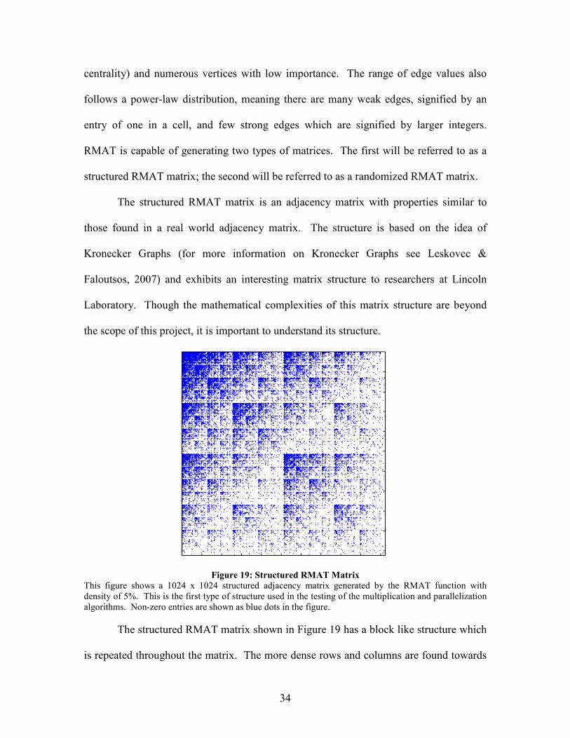
RMAT is capable of generating two types of matrices. The first will be referred to as a
structured RMAT matrix; the second will be referred to as a randomized RMAT matrix.
The structured RMAT matrix is an adjacency matrix with properties similar to
those found in a real world adjacency matrix. The structure is based on the idea of
Kronecker Graphs (for more information on Kronecker Graphs see Leskovec &
Faloutsos, 2007) and exhibits an interesting matrix structure to researchers at Lincoln
Laboratory. Though the mathematical complexities of this matrix structure are beyond
the scope of this project, it is important to understand its structure.
Figure 19: Structured RMAT Matrix
This figure shows a 1024 x 1024 structured adjacency matrix generated by the RMAT function with
density of 5%. This is the first type of structure used in the testing of the multiplication and parallelization
algorithms. Non-zero entries are shown as blue dots in the figure.
The structured RMAT matrix shown in Figure 19 has a block like structure which
is repeated throughout the matrix. The more dense rows and columns are found towards
35
the left and upper parts of the matrix. This same structure is repeated in smaller and
smaller blocks throughout the entire structure. Because of this block structure, dense
rows and columns are repeated at constant intervals throughout the matrix.
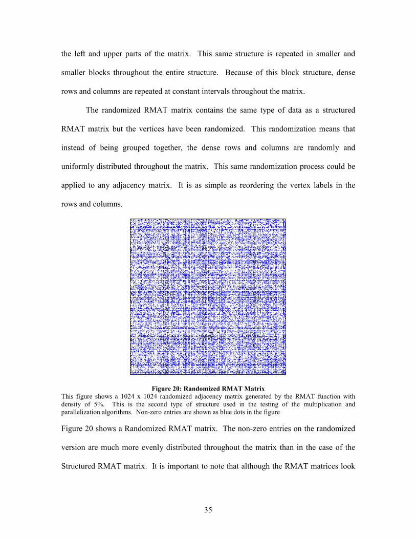
The randomized RMAT matrix contains the same type of data as a structured
RMAT matrix but the vertices have been randomized. This randomization means that
instead of being grouped together, the dense rows and columns are randomly and
uniformly distributed throughout the matrix. This same randomization process could be
applied to any adjacency matrix. It is as simple as reordering the vertex labels in the
rows and columns.
Figure 20: Randomized RMAT Matrix
This figure shows a 1024 x 1024 randomized adjacency matrix generated by the RMAT function with
density of 5%. This is the second type of structure used in the testing of the multiplication and
parallelization algorithms. Non-zero entries are shown as blue dots in the figure
Figure 20 shows a Randomized RMAT matrix. The non-zero entries on the randomized
version are much more evenly distributed throughout the matrix than in the case of the
Structured RMAT matrix. It is important to note that although the RMAT matrices look
36
as though they might be symmetric across the major diagonal, they are unidirectional
adjacency matrices and not symmetric.
2.4 Field Programmable Gate Arrays (FPGAs)
A final deliverable of this project was to parallelize the optimized sparse matrix
multiply algorithm on a field-programmable gate array (FPGA). An FPGA is a type of
programmable logic device (PLD) with which an engineer can develop almost any logic
circuit s/he wishes, or even multiple copies of the same logic circuit. Using multiple
copies of a specialized logic circuit enables an FPGA to perform operations
simultaneously, thus processing data in parallel. Implementing parallel processing on a
single chip gives a large advantage over an array of conventional microprocessors which
is slowed by inefficient communication. Inside an FPGA, separate circuits have high
connectivity and can transmit data between each other quickly and efficiently.
Research has shown that the implementation of an FPGA with multiple
interconnected copies of the same circuit can parallelize operations and achieve “almost
supercomputer-class performance” at a “tiny fraction of the cost of more general-purpose
supercomputing hardware” (Pellerin, and Thibault, 2005). FPGAs enable developers to
design a circuit which performs exactly the computations they need it to and nothing
more. By parallelizing and optimizing for one algorithm, a device can be made much
more capable to perform its job; however, this optimization simultaneously makes it less
versatile:
Parallel architectures can be more powerful, but are less general. A special-
purpose circuit can always outperform a microprocessor-based implementation
for a small class of problems ….The very specialization which provides this
parallelism also necessarily limits the range of its application.(Oldfield & Dorf,
1995)
37
FPGA’s are often a good choice for the development of a complicated yet
dedicated hardware circuit. Once a system becomes massively produced, implementing
it on an Application Specific Integrated Circuit (ASIC) is usually more economical and
can provide another level of optimization above the FPGA.
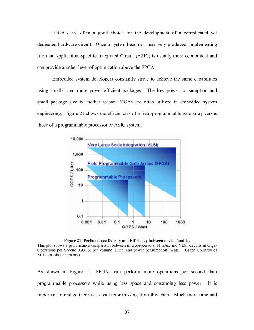
Embedded system developers constantly strive to achieve the same capabilities
using smaller and more power-efficient packages. The low power consumption and
small package size is another reason FPGAs are often utilized in embedded system
engineering. Figure 21 shows the efficiencies of a field-programmable gate array versus
those of a programmable processor or ASIC system.
Figure 21: Performance Density and Efficiency between device families
This plot shows a performance comparison between microprocessors, FPGAs, and VLSI circuits in Giga-
Operations per Second (GOPS) per volume (Liter) and power consumption (Watt). (Graph Courtesy of
MIT Lincoln Laboratory)
As shown in Figure 21, FPGAs can perform more operations per second than
programmable processors while using less space and consuming less power. It is
important to realize there is a cost factor missing from this chart. Much more time and
38
money will be spent to develop an FPGA solution to a problem rather than using a
programmable processor. Even more resources will be needed to develop a Very Large
Scale Integration (VLSI) implementation such as an ASIC. There is a direct relation
between time, cost, level of development, and performance. For this project, achieving
the performance of an FPGA implementation is a reasonable target for the available time
and resources.
2.4.1 FPGA Architecture
An FPGA is a reprogrammable semiconductor device which is becoming very
commonly used in the development of embedded systems. Its ability to be
reprogrammed in the field is unlike other programmable logic devices which, once
configured, cannot be changed. On an FPGA, an engineer can implement almost any
type of logic circuit. These logic circuits are implemented by using a hardware definition
language (HDL) like Verilog or VHDL. The range of implementation can range from a
simple logic gate such as an OR or an AND gate to extremely complex circuits. Figure
22 shows a diagram of the basic structure inside an FPGA.
39
Figure 22: FPGA Architecture
This figure shows the inner architecture of a basic FPGA. The blue blocks in the middle are Configurable
Logic Blocks (CLBs), while the red blocks on the outer edges are I/O blocks. Between the blocks, in
yellow, are the row and column programmable interconnects. (Floyd, 2006)
The inside of an FPGA is mainly comprised of a grid of programmable logic
blocks and interconnections. By combining a number of these blocks and connecting
them through the grid of programmable interconnects, the FPGA can take on the role of
almost any logic circuit. A single programmable logic block consists of a Look-Up Table
(LUT), a D Flip-Flop connected to the main clock of the device, and output logic
(Computer Engineering Research Group, University of Toronto, 2007). Figure 23 shows
the basic internal structure of a programmable logic block.
40
Figure 23: FPGA Logic Block
This figure shows the inner workings of a Configurable Logic Block. It consists of a Look-Up Table
(LUT), a D flip flop and output logic. (Cofer & Harding, 2006)
The I/O blocks on an FPGA are also configured by the user. These blocks control how
and where information is transferred in and out of the FPGA (which pin or pins the inputs
are read through and the outputs are sent through). Modern FPGAs often have other
hardware devices embedded in them such as block RAM, Universal Asynchronous
Receiver-Transmitters (UARTs) or even PowerPC processors.
Many Intellectual Property (IP) or soft-cores can be implemented on an FPGA as
well. IP cores are files written in a Hardware Definition Language (HDL) which can be
obtained through various sources and perform a specific application. An engineer would
have to load the HDL file onto the FPGA. There is a large variety of IP or Soft-cores
available that perform commonly used circuits. A quick internet search can find
41
downloadable IP cores for encryptions, Fast Fourier Transforms (FFTs), USB controllers
or even microprocessors. This high degree of versatility and performance is why FPGAs
are often a good choice for embedded systems engineers.
2.4.2 Soft-Core Microprocessors
Embedding a soft-core processor can reduce the time and effort involved in
designing an embedded system with an FPGA. A soft-core processor is an entire
microprocessor implemented in the hardware of an FPGA through an HDL file. These
processors can run software, just like the processor in the average desktop computer.
When implementing an algorithm on an FPGA, it is often most cost effective to
implement only the most time-intensive parts of the algorithm in gate-level hardware,
while leaving the less time consuming parts to be completed by software run by a soft-
core processor. Soft-core microprocessors allow an engineer to develop a system on an
FPGA which is a hybrid between hardware and software (Eskowitz et al., 2004). With
the option of a soft-core software implementation, an engineer can decide which parts of
their algorithm will benefit most from a gate-level hardware circuit and which ones are
more efficiently performed by software.
A soft-core microprocessor can also increase a company’s ability for rapid
development and deployment of systems by allowing production and development times
to overlap. An original design of an FPGA could perform most of its functions by a soft-
core processor embedded on the FPGA. The company could begin mass production of a
working product while its engineers were still developing and optimizing the design’s
logic circuits. Later, due to the FPGA’s field programmability, the company could
update its systems with more gate-level hardware implementations. This process could
42
continue until, eventually, the entire design was optimized through gate-level hardware
implementations.
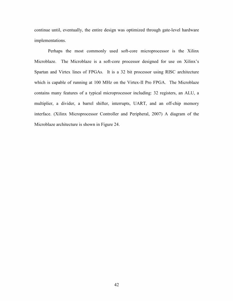
Perhaps the most commonly used soft-core microprocessor is the Xilinx
Microblaze. The Microblaze is a soft-core processor designed for use on Xilinx’s
Spartan and Virtex lines of FPGAs. It is a 32 bit processor using RISC architecture
which is capable of running at 100 MHz on the Virtex-II Pro FPGA. The Microblaze
contains many features of a typical microprocessor including: 32 registers, an ALU, a
multiplier, a divider, a barrel shifter, interrupts, UART, and an off-chip memory
interface. (Xilinx Microprocessor Controller and Peripheral, 2007) A diagram of the
Microblaze architecture is shown in Figure 24.
43
Figure 24: Microblaze Architecture
This figure shows the typical layout and architecture of the Xilinx Microblaze soft-core processor.
(Rosinger, 2004)
The Microblaze is truly designed for use inside an FPGA. Since soft-cores run at much
slower clock speeds than a hard-core processor, the primary reason for using a soft-core
on an FPGA would be to use it in conjunction with other IP that can speed up the
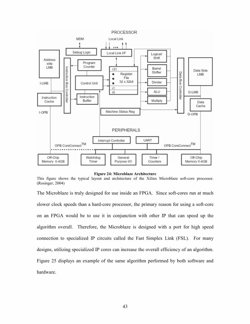
algorithm overall. Therefore, the Microblaze is designed with a port for high speed
connection to specialized IP circuits called the Fast Simplex Link (FSL). For many
designs, utilizing specialized IP cores can increase the overall efficiency of an algorithm.
Figure 25 displays an example of the same algorithm performed by both software and
hardware.
44
Figure 25: Software Algorithm vs. Hardware
This figure shows the same process performed by a microprocessor in software on the left and by a
hardware circuit on the right. A, B, C, D, E, F, and G are assumed to be numeric values stored in the
memory of the system. (Rosinger, 2004)
The hardware solution of this algorithm requires two clock cycles while the
software requires 12. A specialized logic circuit is often the best choice for speeding up
complicated functions in an FPGA design and often provides motivation for a soft-core
processor to outsource some of its more time consuming jobs to hardware.
2.4.3 PowerPC processor
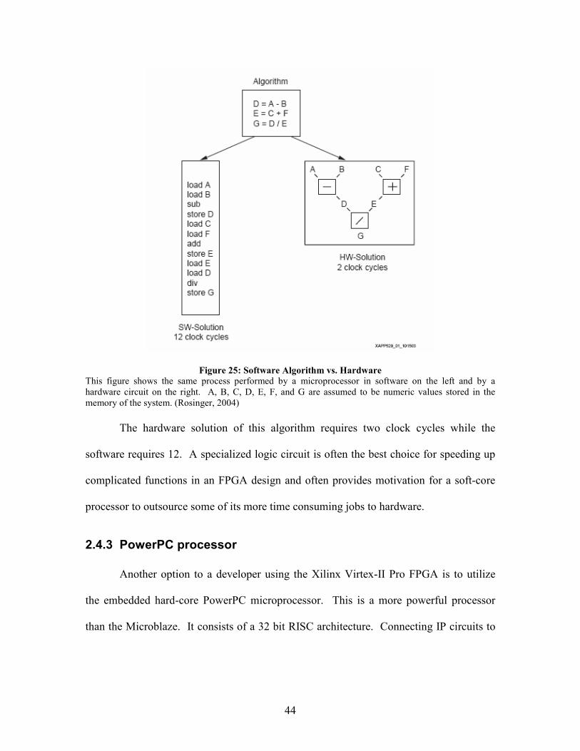
Another option to a developer using the Xilinx Virtex-II Pro FPGA is to utilize
the embedded hard-core PowerPC microprocessor. This is a more powerful processor
than the Microblaze. It consists of a 32 bit RISC architecture. Connecting IP circuits to
45
the PowerPC is different than in the Microblaze. Any IP cores utilized by the PowerPC
are connected through the On-Chip Peripheral Bus rather than the Fast Simplex Link.
Figure 26: PowerPC Architecture
This figure shows an example of an embedded system utilizing an embedded PowerPC microprocessor on a
Xilinx FPGA. (Xilinx PowerPC 405 Processor, 2007)
The embedded PowerPC will not be used in our hardware implementation, but it is
available for future use.
2.5 ML310 Development Board
The FPGA board that the final design of this project was implemented on is
Xilinx’s ML310 development board. The ML310 is a board meant for rapid system
prototyping of embedded systems using the Virtex-II Pro FPGA. The ML310 comes
standard with a Xilinx Virtex-II Pro XC2VP30 chip. It also comes with a myriad of
peripheral devices such as USB ports, parallel and serial connections, IDE connections
for hard drives or CD ROMs, an LCD interface, LEDs, a UART connector to send out
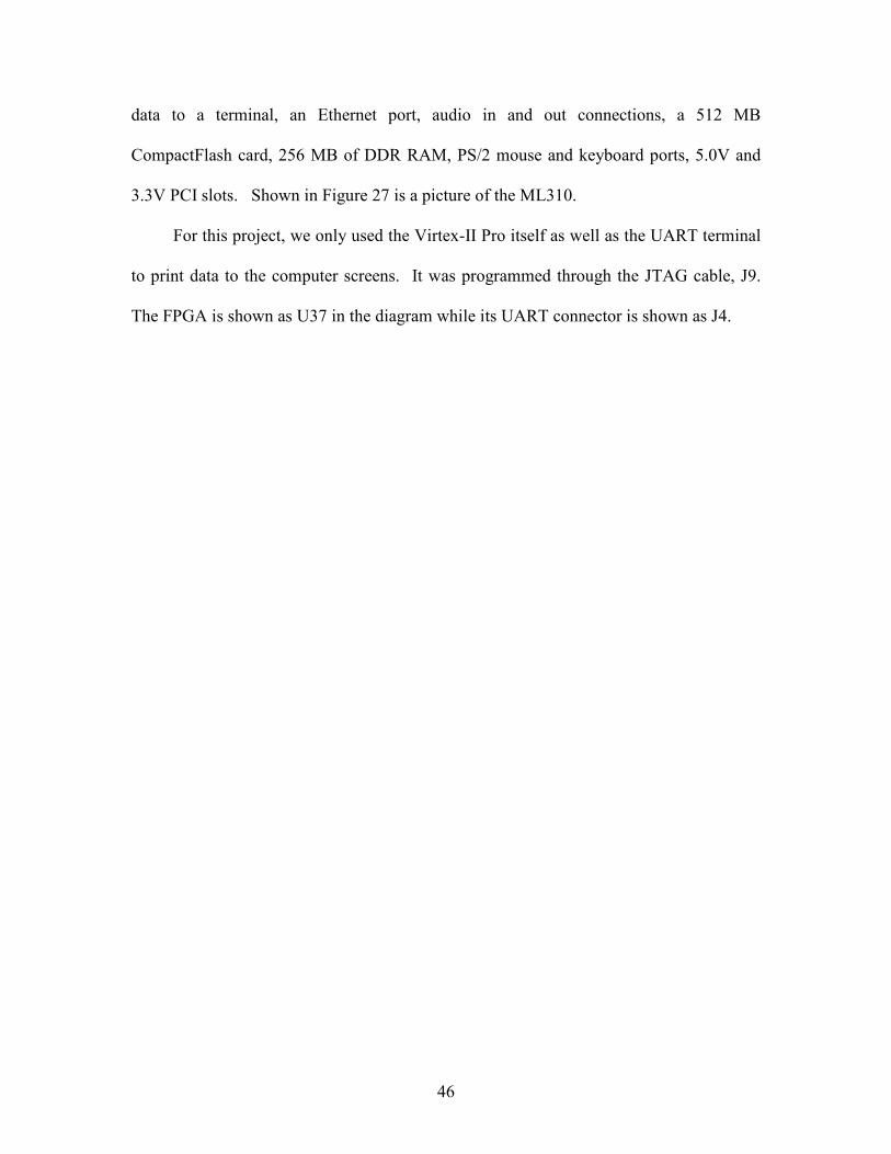
46
data to a terminal, an Ethernet port, audio in and out connections, a 512 MB
CompactFlash card, 256 MB of DDR RAM, PS/2 mouse and keyboard ports, 5.0V and
3.3V PCI slots. Shown in Figure 27 is a picture of the ML310.
For this project, we only used the Virtex-II Pro itself as well as the UART terminal
to print data to the computer screens. It was programmed through the JTAG cable, J9.
The FPGA is shown as U37 in the diagram while its UART connector is shown as J4.
47
Figure 27: Xilinx ML310 Development Board
This figure is a diagram showing the Xilinx ML310 development board. The board is used for rapid
embedded system prototyping and comes with many useable peripherals. The Virtex-II Pro FPGA is
shown above as U37. The UART port we used to print text to our screen is marked J4 while the JTAG
connector used to program the Virtex is marked at the top as J9. (ML310 User Guide)
48
2.6 Xilinx Virtex-II Pro XC2VP30
The Virtex-II Pro XC2VP30 is a high performance FPGA platform developed by
Xilinx Inc., a leading FPGA manufacturer. The Virtex-II Pro line of FPGAs is targeted
towards communication and DSP applications and is manufactured using a 0.13 µm
CMOS nine-layer copper process. The XC2VP30 model contains 30,816 logic cells,
each consisting of a 4-input look-up table, a flip-flop, and carry logic. It also contains
136 18x18 bit multipliers and 136 blocks of RAM of 2.25 KB each; making the total
RAM available 306 KB.
Furthermore, it contains eight RocketIO transceiver blocks which are responsible for
high speed connectivity and conversions between parallel and serial interfaces. Two
hard-core PowerPC microprocessors (400MHz) are also embedded on the XC2VP30.
The Microblaze soft-core processor can also be implemented in the logic of the
XC2VP30. An implementation of the Microblaze on this FPGA can run at a clock speed
of 100MHz. (Virtex-II Pro Data Sheet)
49
3 Algorithm Performance Analysis
There are multiple techniques an engineering team could pursue when building
and parallelizing an optimal sparse matrix multiplication algorithm. Because of the many
options and the inherent memory constraints on an FPGA, we sought an algorithm which
would both perform multiplication quickly and efficiently while keeping memory
requirements to a minimum. The methodology section discusses the processes of both
optimizing a multiplication algorithm and implementing the algorithm on an FPGA.
When developing the FPGA algorithm, multiple methods for the storage and
multiplication of two sparse matrices were simulated in MATLAB to find a technique
that both compressed the matrices effectively and performed the multiplication at a
higher efficiency than a full matrix multiplication. After determining the formats and
algorithm for optimized multiplication, load distribution methods were simulated to find
one that efficiently parallelized the multiplication between multiple processing elements.
3.1 Optimized Matrix Multiplication Algorithm
To multiply a set of two matrices, a certain number of calculations must be
performed regardless of storage type and indexing method. These calculations are the
non-zero arithmetic operations; multiplying and summing the corresponding values in a
row of matrix A and a column of matrix B. Each type of matrix multiplication has some
overhead involved in performing these non-zero calculations. In the case of full matrix
multiplication, the overhead takes the form of multiple zero operations (multiplying by a
zero or adding zero) that are not important to product. In the case of sparse matrix
multiplications, the overhead takes the form of more complicated indexing and searching
50
operations which find the intersecting values to be multiplied. The most efficient
multiplication method will perform these non-zero operations with the least amount of
overhead.
To determine the most efficient method to store and multiply two sparse matrices
for multiplication, storage methods from those discussed in the background were tested to
find one with high multiplicational efficiency and maximum compression of the matrices.
The definition of efficiency we used was the number of non-zero operations divided by
the maximum possible number of non-zero operations performed by the processor. The
target matrices were adjacency matrices with less than 5% density. Four separate storage
methods were tested to find a combination which organized the matrices optimally for
multiplication.
Four different multiplication algorithms were tested for efficiency in MATLAB.
Because MATLAB itself utilizes C functions to perform some of its calculations faster,
none of the test functions ran faster than MATLAB’s embedded matrix multiplication
functions. The tests sought to test different multiplication methods against each other on
the same level of development. MATLAB served as the common platform upon which
all algorithms were built. Testing these algorithms in MATLAB provided an estimate of
their relative efficiencies in other programming languages such as C or even hardware
definition languages like VHDL.
During the testing procedures, the efficiency of each algorithm was calculated.
To measure efficiency, two RMAT test matrices with dimensions 1024x1024 were
generated for each density tested (1% to 99%). The total number of non-zero
calculations (multiplications and additions) to multiply the two test matrices was counted
51
using a specialized function we developed. The multiplication was timed, and the
number of calculations was divided by the total time. The performance of each
algorithm, in non-zero operations per second, was divided by the clock speed of the
processor, giving the efficiency of the algorithm. A plot was generated showing the
efficiency of each matrix multiplication in non-zero operations per second.
These tests were run on machines with the same hardware specifications to ensure
their consistency. During testing, the machines were monitored to ensure there was no
additional CPU load unrelated to testing. The machines were Quad core 3.066 GHz
processors with 2.5 Gigabytes of RAM each; part of the MIT-Lincoln Laboratory group
102 cluster. Five instances of each matrix multiplication test were run and averaged.
The test’s goal was to determine which multiplication method performed most efficiently
on the target matrices and to determine the range of densities for which these methods
performed at higher efficiency than a full matrix multiplication. The plot made strong
suggestions as to which algorithm worked with the least overhead.
3.1.1 Full Matrix Multiplication
To multiply two full matrices in a full matrix storage format, a function was
developed in MATLAB so each sparse method could be compared against it. Because all
the RMAT matrices were originally stored in a full format, tests could easily be run on
these matrices before converting them to various sparse formats to be tested. A full
matrix multiplication stores and multiplies all entries inside the matrices regardless of
whether they’re zero or not. Building our own full matrix multiplication function
allowed our plots to show the benefits of multiplication in the sparse domain versus the
full domain.
52
MATLAB does have its own full matrix times full matrix function built in
(matrixA*matrixB), but MATLAB’s function utilizes C-code which operates on a much
lower level than MATLAB and is much faster. MATLAB’s function would not be
comparable to the sparse matrix multiplication methods which were tested. We therefore
built our own function in MATLAB which would be comparable.
3.1.1.1 Full Matrix Multiplication Algorithm
The following is pseudocode showing the full matrix multiplication algorithm
which was tested:
for (x=1; x<matrixA.row; x++) //<- cycle for every row in A for (y=1; y<matrixB.column; y++)) //<- cycle by column in B Compute dot product of Row x in A and Column y in B Write result to entry (x,y) in resultant matrix end end
This process cycles through the rows of A and the columns of B performing vector by
vector multiplication. The dot product of each row by each column is computed and the
answer is written to the corresponding cell in matrix C. The actual MATLAB code used
for the simulation can be found in Appendix A.
3.1.2 Sparse Matrix Multiplication
When a sparsely populated matrix is multiplied in a full fashion, many
unnecessary zero operations (multiplying by zero or adding with zero) are performed. By
storing the matrices in a sparse format, these operations are eliminated and only useful
operations are performed. The disadvantage of using sparse matrix storage to multiply is
that the multiplication algorithm takes on an overhead of more complicated indexing and
53
searching operations. In basic sparse matrix storage format each matrix is sorted by
column. Sorting by column means values in the same row are not stored near each other
in memory and the algorithm must perform extensive searching to find the row values it
needs to multiply.
3.1.2.1 Sparse Matrix Multiplication Algorithm
The following is the pseudocode showing the algorithm for the multiplication of
two sparse matrices stored in a basic sparse matrix format (both sorted by column).
for (x=1; x<matrixB.column; x++) //<- cycle by column in B determine appropriate column indices (determine how many indices there are) for (y=1; y<matrixA.row; y++)) //<- cycle by row in A determine appropriate row indices (search for all the appropriate indices) determine matching indices vector multiplication assign final values end end
The actual MATLAB code used for the simulation can be found in Appendix A.
3.1.3 Sorted Sparse Matrix Multiplication
In sorted sparse matrix multiplication, only non-zero values are computed as in
the basic sparse multiplication, but each matrix is sorted in an optimal way for
multiplication to be performed. Because matrix multiplication multiplies the rows of
matrix A by the columns of matrix B, it is most efficient to store matrix A sorted by row
and matrix B sorted by column. When finding the values in a row or column, no
searching operations are needed, only counting of the indices.
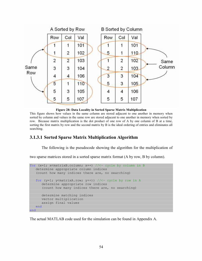
54
Figure 28: Data Locality in Sorted Sparse Matrix Multiplication
This figure shows how values in the same column are stored adjacent to one another in memory when
sorted by column and values in the same row are stored adjacent to one another in memory when sorted by
row. Because matrix multiplication is the dot product of one row of A by one column of B at a time,
sorting the first matrix by row and the second matrix by B is the ideal ordering of entries and eliminates all
searching.
3.1.3.1 Sorted Sparse Matrix Multiplication Algorithm
The following is the pseudocode showing the algorithm for the multiplication of
two sparse matrices stored in a sorted sparse matrix format (A by row, B by column).
for (x=1; x<matrixB.column; x++) //<- cycle by column in B determine appropriate column indices (count how many indices there are, no searching) for (y=1; y<matrixA.row; y++)) //<- cycle by row in A determine appropriate row indices (count how many indices there are, no searching) determine matching indices vector multiplication assign final values end end
The actual MATLAB code used for the simulation can be found in Appendix A.
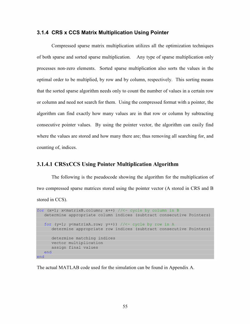
55
3.1.4 CRS x CCS Matrix Multiplication Using Pointer
Compressed sparse matrix multiplication utilizes all the optimization techniques
of both sparse and sorted sparse multiplication. Any type of sparse multiplication only
processes non-zero elements. Sorted sparse multiplication also sorts the values in the
optimal order to be multiplied, by row and by column, respectively. This sorting means
that the sorted sparse algorithm needs only to count the number of values in a certain row
or column and need not search for them. Using the compressed format with a pointer, the
algorithm can find exactly how many values are in that row or column by subtracting
consecutive pointer values. By using the pointer vector, the algorithm can easily find
where the values are stored and how many there are; thus removing all searching for, and
counting of, indices.
3.1.4.1 CRSxCCS Using Pointer Multiplication Algorithm
The following is the pseudocode showing the algorithm for the multiplication of
two compressed sparse matrices stored using the pointer vector (A stored in CRS and B
stored in CCS).
for (x=1; x<matrixB.column; x++) //<- cycle by column in B determine appropriate column indices (subtract consecutive Pointers) for (y=1; y<matrixA.row; y++)) //<- cycle by row in A determine appropriate row indices (subtract consecutive Pointers) determine matching indices vector multiplication assign final values end end
The actual MATLAB code used for the simulation can be found in Appendix A.
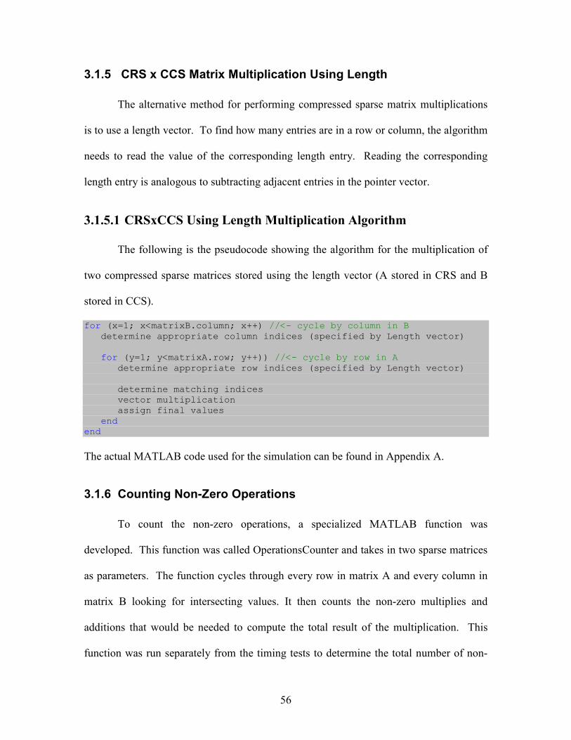
56
3.1.5 CRS x CCS Matrix Multiplication Using Length
The alternative method for performing compressed sparse matrix multiplications
is to use a length vector. To find how many entries are in a row or column, the algorithm
needs to read the value of the corresponding length entry. Reading the corresponding
length entry is analogous to subtracting adjacent entries in the pointer vector.
3.1.5.1 CRSxCCS Using Length Multiplication Algorithm
The following is the pseudocode showing the algorithm for the multiplication of
two compressed sparse matrices stored using the length vector (A stored in CRS and B
stored in CCS).
for (x=1; x<matrixB.column; x++) //<- cycle by column in B determine appropriate column indices (specified by Length vector) for (y=1; y<matrixA.row; y++)) //<- cycle by row in A determine appropriate row indices (specified by Length vector) determine matching indices vector multiplication assign final values end end
The actual MATLAB code used for the simulation can be found in Appendix A.
3.1.6 Counting Non-Zero Operations
To count the non-zero operations, a specialized MATLAB function was
developed. This function was called OperationsCounter and takes in two sparse matrices
as parameters. The function cycles through every row in matrix A and every column in
matrix B looking for intersecting values. It then counts the non-zero multiplies and
additions that would be needed to compute the total result of the multiplication. This
function was run separately from the timing tests to determine the total number of non-
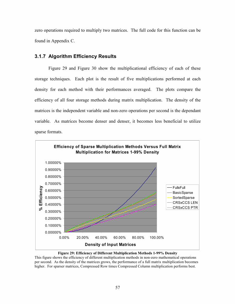
57
zero operations required to multiply two matrices. The full code for this function can be
found in Appendix C.
3.1.7 Algorithm Efficiency Results
Figure 29 and Figure 30 show the multiplicational efficiency of each of these
storage techniques. Each plot is the result of five multiplications performed at each
density for each method with their performances averaged. The plots compare the
efficiency of all four storage methods during matrix multiplication. The density of the
matrices is the independent variable and non-zero operations per second is the dependant
variable. As matrices become denser and denser, it becomes less beneficial to utilize
sparse formats.
Efficiency of Sparse Multiplication Methods Versus Full Matrix
Multiplication for Matrices 1-99% Density
0.00000%
0.10000%
0.20000%
0.30000%
0.40000%
0.50000%
0.60000%
0.70000%
0.80000%
0.90000%
1.00000%
0.00% 20.00% 40.00% 60.00% 80.00% 100.00%
Density of Input Matrices
% Efficiency FullxFull
BasicSparse
SortedSparse
CRSxCCS LEN
CRSxCCS PTR
Figure 29: Efficiency of Different Multiplication Methods 1-99% Density
This figure shows the efficiency of different multiplication methods in non-zero mathematical operations
per second. As the density of the matrices grows, the performance of a full matrix multiplication becomes
higher. For sparser matrices, Compressed Row times Compressed Column multiplication performs best.
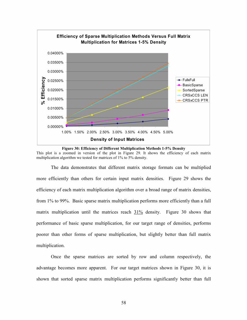
58
Efficiency of Sparse Multiplication Methods Versus Full Matrix
Multiplication for Matrices 1-5% Density
0.00000%
0.00500%
0.01000%
0.01500%
0.02000%
0.02500%
0.03000%
0.03500%
0.04000%
1.00% 1.50% 2.00% 2.50% 3.00% 3.50% 4.00% 4.50% 5.00%
Density of Input Matrices
% Efficiency
FullxFull
BasicSparse
SortedSparse
CRSxCCS LEN
CRSxCCS PTR
Figure 30: Efficiency of Different Multiplication Methods 1-5% Density
This plot is a zoomed in version of the plot in Figure 29. It shows the efficiency of each matrix
multiplication algorithm we tested for matrices of 1% to 5% density.
The data demonstrates that different matrix storage formats can be multiplied
more efficiently than others for certain input matrix densities. Figure 29 shows the
efficiency of each matrix multiplication algorithm over a broad range of matrix densities,
from 1% to 99%. Basic sparse matrix multiplication performs more efficiently than a full
matrix multiplication until the matrices reach 31% density. Figure 30 shows that
performance of basic sparse multiplication, for our target range of densities, performs
poorer than other forms of sparse multiplication, but slightly better than full matrix
multiplication.
Once the sparse matrices are sorted by row and column respectively, the
advantage becomes more apparent. For our target matrices shown in Figure 30, it is
shown that sorted sparse matrix multiplication performs significantly better than full
59
matrix multiplication and basic sparse matrix multiplication. For higher densities, in
Figure 29, sorted sparse multiplication performs better than full matrix multiplication
until the density of the input matrices reaches 45%. These plots illustrate the advantage
given by the optimal sorting of the matrices.
A final leap in efficiency is achieved once the compressed formats are
implemented and both searching and counting operations are eliminated completely. The
two types of compressed multiplications (utilizing the Length vector and using the
Pointer Vector) performed similarly for the matrices of interest to this project as shown in
Figure 30. CRSxCCS multiplication using the pointer vector performed only slightly
better on average than using the length vector. For densities of up to 99%, both
CRSxCCS multiplications performed significantly better than all other methods until the
input density reaches about 53%, at which point full matrix multiplication became more
efficient. From these numbers, it is clear that compressed sparse matrix multiplication is
the most efficient method. Because of their similar efficiencies, the decision of whether
to use the length or pointer vector depended on each storage format’s functionality during
parallelization of the multiplication algorithm.
3.2 Optimized Parallelization and Load Balancing Technique
In section 3.1.7 it was shown why we chose compressed row times compressed
column formats in which to store our matrices. Because of the way the matrices were
sorted, the ways we could easily split the matrices for parallelization were limited. We
could either split matrix A into submatrices of its rows or matrix B into submatrices of its
columns. Splitting both of these matrices simultaneously was not feasible since it would
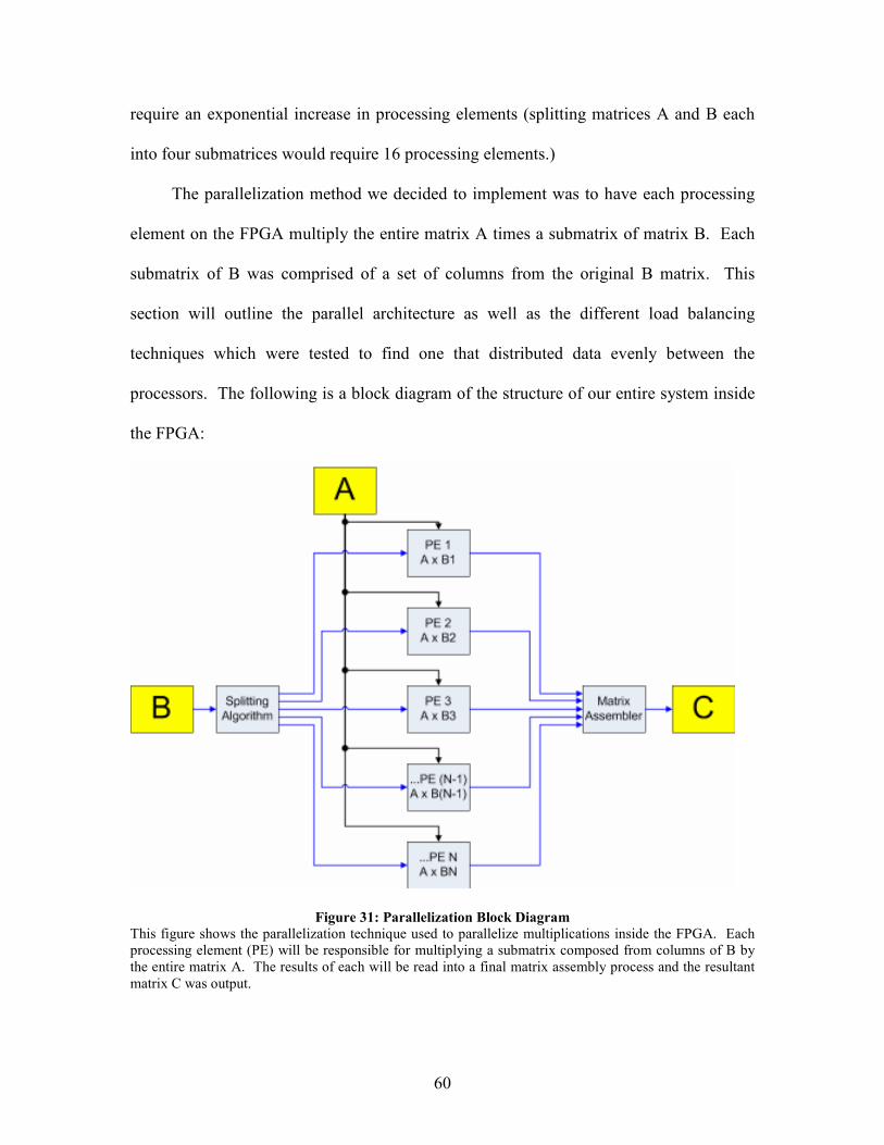
60
require an exponential increase in processing elements (splitting matrices A and B each
into four submatrices would require 16 processing elements.)
The parallelization method we decided to implement was to have each processing
element on the FPGA multiply the entire matrix A times a submatrix of matrix B. Each
submatrix of B was comprised of a set of columns from the original B matrix. This
section will outline the parallel architecture as well as the different load balancing
techniques which were tested to find one that distributed data evenly between the
processors. The following is a block diagram of the structure of our entire system inside
the FPGA:
Figure 31: Parallelization Block Diagram
This figure shows the parallelization technique used to parallelize multiplications inside the FPGA. Each
processing element (PE) will be responsible for multiplying a submatrix composed from columns of B by
the entire matrix A. The results of each will be read into a final matrix assembly process and the resultant
matrix C was output.
61
As shown in the graphic above, matrix A will be supplied to each processing
element as soon as it enters the FPGA. Matrix B will be split into N submatrices by a
splitting algorithm (N is the number of processing elements on the chip). Each
processing element will multiply A by a submatrix of B producing a submatrix of C. The
result will then be combined by a final matrix assembly algorithm and the resultant
matrix, C will be output from the FPGA.
To work effectively, a parallel architecture needs a method for distributing
computations evenly between processors. The following sections will discuss the type of
multiplication we chose to implement and why it is better for parallelization. The tests
performed on various load distribution techniques will also be discussed.
3.2.1 Pointer vs. Length Vector in Parallelization
In the multiplication testing section, both compressed sparse matrix storage
techniques (using the pointer vector and using the length vector) performed similarly.
This comparable performance between the two formats differs once parallelization is
considered. The differences in parallel performance using each storage method will be
outlined in this section.
During parallelization of the multiplication algorithm, matrices are broken down
into smaller matrices for distribution to individual processing elements. When dividing
compressed sparse matrices, matrices stored using a pointer vector and matrices stored
using a length vector require different operations when splitting. An example is shown
below of how these storage methods differ.
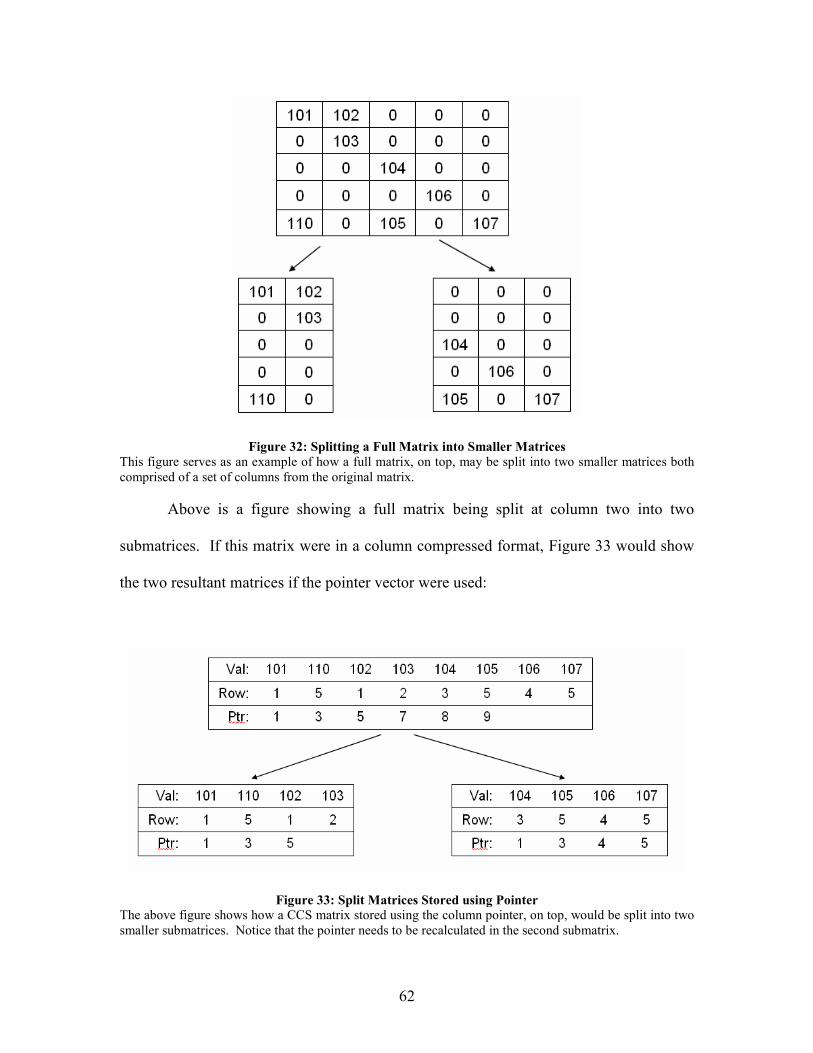
62
Figure 32: Splitting a Full Matrix into Smaller Matrices
This figure serves as an example of how a full matrix, on top, may be split into two smaller matrices both
comprised of a set of columns from the original matrix.
Above is a figure showing a full matrix being split at column two into two
submatrices. If this matrix were in a column compressed format, Figure 33 would show
the two resultant matrices if the pointer vector were used:
Figure 33: Split Matrices Stored using Pointer
The above figure shows how a CCS matrix stored using the column pointer, on top, would be split into two
smaller submatrices. Notice that the pointer needs to be recalculated in the second submatrix.
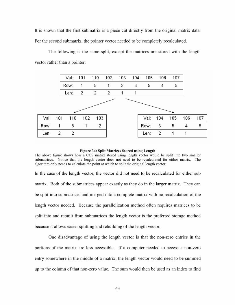
63
It is shown that the first submatrix is a piece cut directly from the original matrix data.
For the second submatrix, the pointer vector needed to be completely recalculated.
The following is the same split, except the matrices are stored with the length
vector rather than a pointer:
Figure 34: Split Matrices Stored using Length
The above figure shows how a CCS matrix stored using length vector would be split into two smaller
submatrices. Notice that the length vector does not need to be recalculated for either matrix. The
algorithm only needs to calculate the point at which to split the original length vector.
In the case of the length vector, the vector did not need to be recalculated for either sub
matrix. Both of the submatrices appear exactly as they do in the larger matrix. They can
be split into submatrices and merged into a complete matrix with no recalculation of the
length vector needed. Because the parallelization method often requires matrices to be
split into and rebuilt from submatrices the length vector is the preferred storage method
because it allows easier splitting and rebuilding of the length vector.
One disadvantage of using the length vector is that the non-zero entries in the
portions of the matrix are less accessible. If a computer needed to access a non-zero
entry somewhere in the middle of a matrix, the length vector would need to be summed
up to the column of that non-zero value. The sum would then be used as an index to find
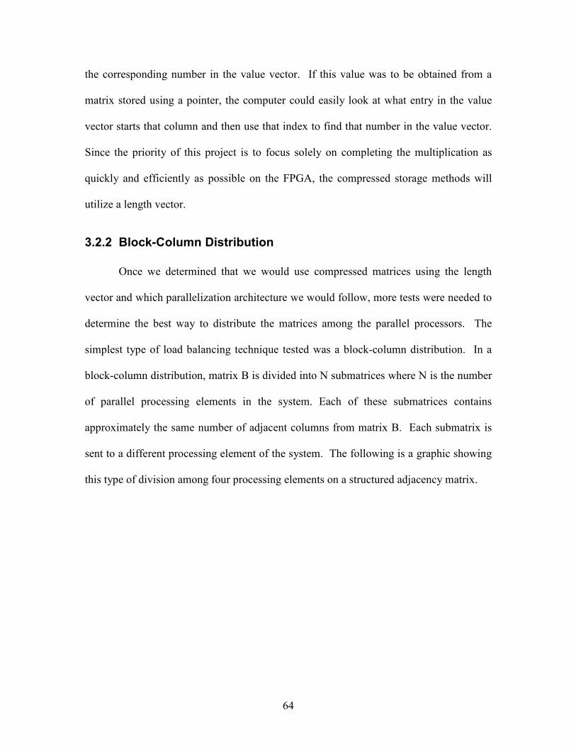
64
the corresponding number in the value vector. If this value was to be obtained from a
matrix stored using a pointer, the computer could easily look at what entry in the value
vector starts that column and then use that index to find that number in the value vector.
Since the priority of this project is to focus solely on completing the multiplication as
quickly and efficiently as possible on the FPGA, the compressed storage methods will
utilize a length vector.
3.2.2 Block-Column Distribution
Once we determined that we would use compressed matrices using the length
vector and which parallelization architecture we would follow, more tests were needed to
determine the best way to distribute the matrices among the parallel processors. The
simplest type of load balancing technique tested was a block-column distribution. In a
block-column distribution, matrix B is divided into N submatrices where N is the number
of parallel processing elements in the system. Each of these submatrices contains
approximately the same number of adjacent columns from matrix B. Each submatrix is
sent to a different processing element of the system. The following is a graphic showing
this type of division among four processing elements on a structured adjacency matrix.
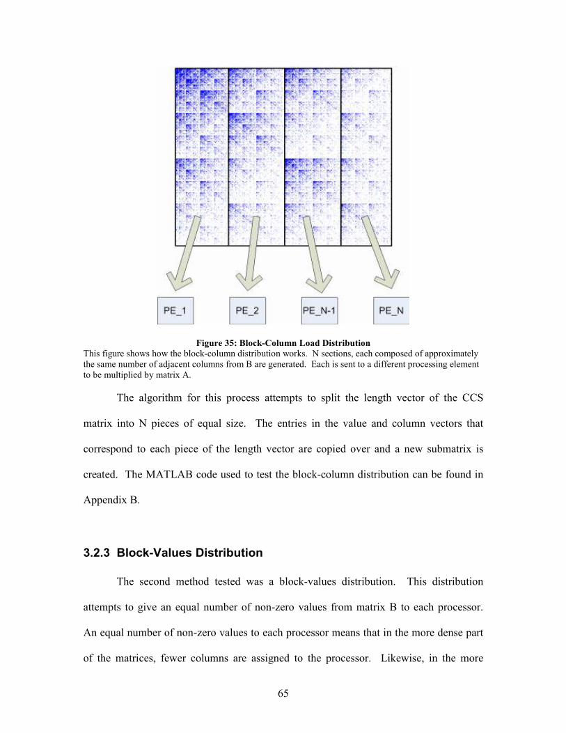
65
Figure 35: Block-Column Load Distribution
This figure shows how the block-column distribution works. N sections, each composed of approximately
the same number of adjacent columns from B are generated. Each is sent to a different processing element
to be multiplied by matrix A.
The algorithm for this process attempts to split the length vector of the CCS
matrix into N pieces of equal size. The entries in the value and column vectors that
correspond to each piece of the length vector are copied over and a new submatrix is
created. The MATLAB code used to test the block-column distribution can be found in
Appendix B.
3.2.3 Block-Values Distribution
The second method tested was a block-values distribution. This distribution
attempts to give an equal number of non-zero values from matrix B to each processor.
An equal number of non-zero values to each processor means that in the more dense part
of the matrices, fewer columns are assigned to the processor. Likewise, in the more
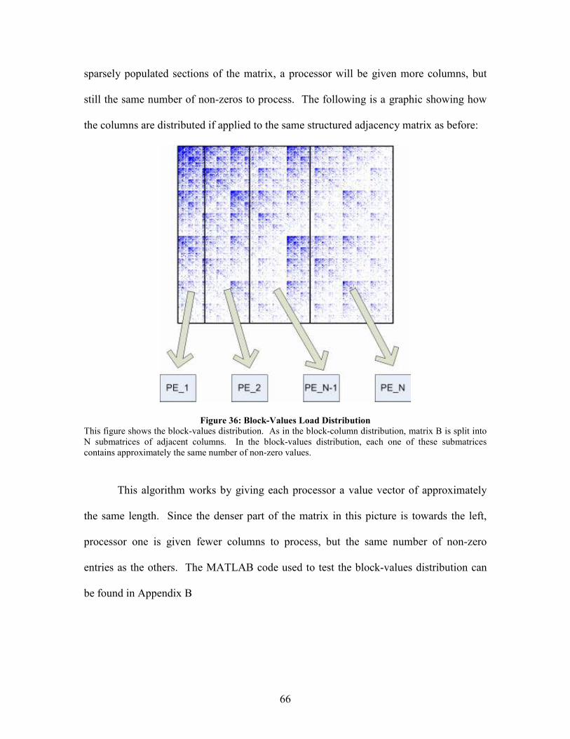
66
sparsely populated sections of the matrix, a processor will be given more columns, but
still the same number of non-zeros to process. The following is a graphic showing how
the columns are distributed if applied to the same structured adjacency matrix as before:
Figure 36: Block-Values Load Distribution
This figure shows the block-values distribution. As in the block-column distribution, matrix B is split into
N submatrices of adjacent columns. In the block-values distribution, each one of these submatrices
contains approximately the same number of non-zero values.
This algorithm works by giving each processor a value vector of approximately
the same length. Since the denser part of the matrix in this picture is towards the left,
processor one is given fewer columns to process, but the same number of non-zero
entries as the others. The MATLAB code used to test the block-values distribution can
be found in Appendix B
67
3.2.4 Block-Cyclic Distribution
A block-cyclic distribution works similarly to the block-column distribution. The
block-cyclic distribution splits the matrix into blocks, each composed of the same number
of columns from B. In block-cyclic distribution, B is split into 2N blocks instead of N.
Each processor is given two of these blocks, one from each half of the matrix. If one side
of the matrix is denser than the other, as is the case in structured adjacency matrices, the
processor will be given both a dense submatrix and a sparser submatrix of B. The blocks
will be distributed between the processing elements in a cyclic manner. Cyclic means
that the blocks are assigned in a repeated sequential order (proc 1, proc 2, proc 3, proc 4).
Once all processors have been assigned one piece of the matrix, the cycle repeats again
until all pieces have been distributed. A cyclic distribution of blocks will help to equalize
the load between all processors. The following is a graphic showing how a block-cyclic
distribution works:
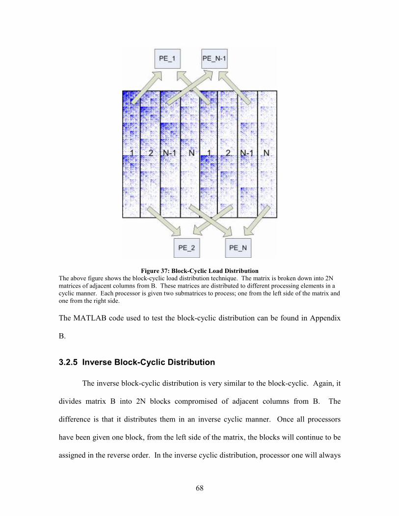
68
Figure 37: Block-Cyclic Load Distribution
The above figure shows the block-cyclic load distribution technique. The matrix is broken down into 2N
matrices of adjacent columns from B. These matrices are distributed to different processing elements in a
cyclic manner. Each processor is given two submatrices to process; one from the left side of the matrix and
one from the right side.
The MATLAB code used to test the block-cyclic distribution can be found in Appendix
B.
3.2.5 Inverse Block-Cyclic Distribution
The inverse block-cyclic distribution is very similar to the block-cyclic. Again, it
divides matrix B into 2N blocks compromised of adjacent columns from B. The
difference is that it distributes them in an inverse cyclic manner. Once all processors
have been given one block, from the left side of the matrix, the blocks will continue to be
assigned in the reverse order. In the inverse cyclic distribution, processor one will always
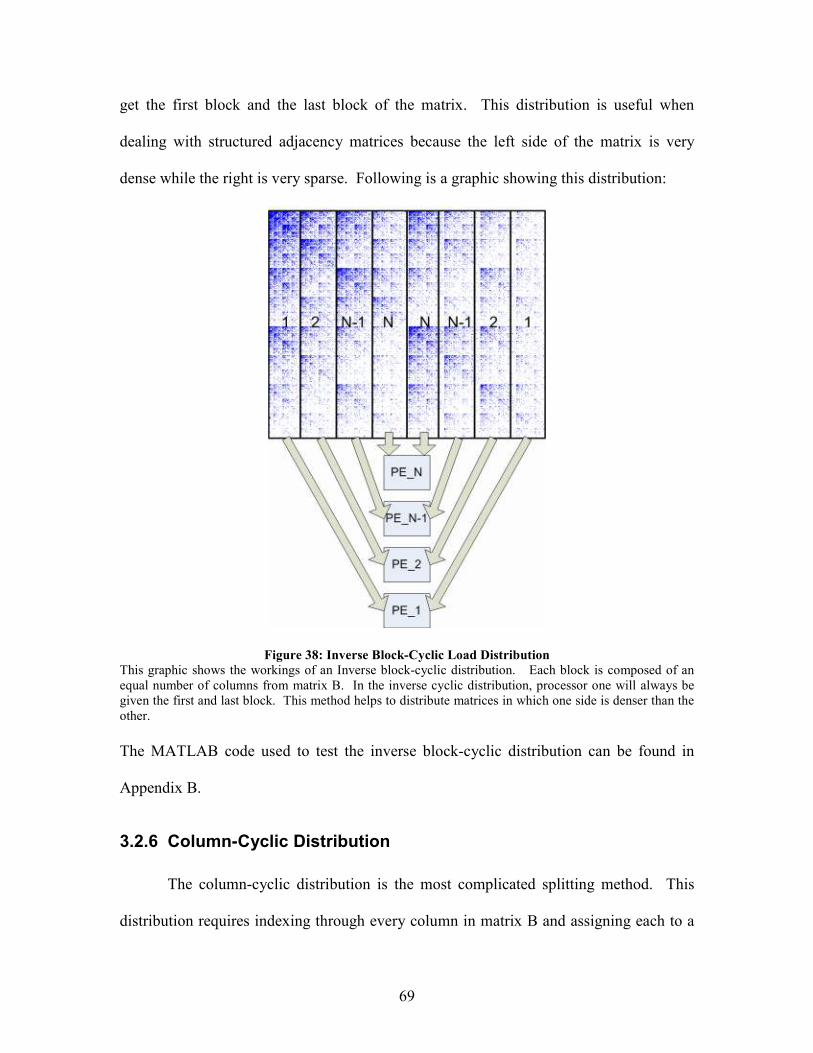
69
get the first block and the last block of the matrix. This distribution is useful when
dealing with structured adjacency matrices because the left side of the matrix is very
dense while the right is very sparse. Following is a graphic showing this distribution:
Figure 38: Inverse Block-Cyclic Load Distribution
This graphic shows the workings of an Inverse block-cyclic distribution. Each block is composed of an
equal number of columns from matrix B. In the inverse cyclic distribution, processor one will always be
given the first and last block. This method helps to distribute matrices in which one side is denser than the
other.
The MATLAB code used to test the inverse block-cyclic distribution can be found in
Appendix B.
3.2.6 Column-Cyclic Distribution
The column-cyclic distribution is the most complicated splitting method. This
distribution requires indexing through every column in matrix B and assigning each to a
70
different processor. The column-cyclic distribution assigns individual columns in a
cyclic manner. The cycling continues until every column in the matrix has been given to
a processor. This method attempts to distribute the dense sections as well as the sparse
sections as evenly as possible between the elements. The cyclic distribution is not easily
shown through a graphic so pseudocode has been generated to show its process.
N=Number of processing elements X=Index of current processing element for (i=1; i<matrixB.column; i++) //<- cycle by column in B X=i mod N; //modular division of current row by N if X==0 //if result of modular division is 0, X=N X=N; Assign row I to processor X; End
As shown by the pseudocode above, the process is very simple, but needs to cycle
for each column in matrix B. The variable X, which determines which processor the
column gets assigned, repeats the series 1, 2, …(N-1), N, 1, 2, …(N-1), N. The modular
division function determines which processor a certain column is assigned. The
MATLAB code used to test the column-cyclic distribution can be found in Appendix B.
3.2.7 Performance Evaluation of Load Balancing Techniques
Tests were run in MATLAB to see the performance of each load balancing
technique on both structured and random adjacency matrices. We were not seeking an
algorithm that performed the best for each type of matrix, rather a more versatile
algorithm that performed reasonably well on both structured and randomized adjacency
matrices. These simulations were not actually run on a parallel system. Instead we
measured the time it took to split up matrix B and reassemble matrix C. In between, we
measured the time it took to multiply each submatrix of matrix B by matrix A
71
individually. The total time was computed by summing the split time, the rebuild time,
and the longest submatrix multiply time.
Once the total time for each computation was found, we again counted the
number of non-zero computations involved in computing the product matrix. The
performance of each load distribution technique was displayed in non-zero operations per
second. In these tests, the size and density of the test matrices were held constant while
the number of simulated processing elements became the independent variable.
3.2.7.1 Performance on Structured Adjacency Matrices
The first set of tests was performed on structured adjacency matrices as discussed
in the background section. The test matrices were 8192 x 8192 adjacency matrices with
1% density. The independent variables in this plot are the number of processors and the
method we used to distribute the load of the multiplication among processing elements.
The dependent variable is the number of non-zero operations per second performed by
the algorithm. Figure 39 shows the average of three runs for each load distribution
method done in MATLAB. The ideal case is also plotted on the graph. The ideal case is
simulated by assuming that the total non-zero computations per second increases linearly
with every processor added; it was extrapolated from the single processor performance.
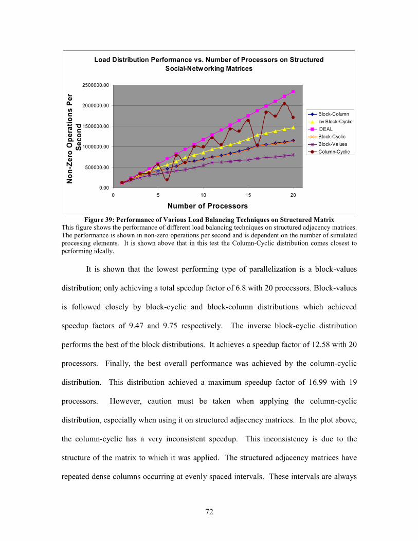
72
Load Distribution Performance vs. Number of Processors on Structured
Social-Networking Matrices
0.00
500000.00
1000000.00
1500000.00
2000000.00
2500000.00
0 5 10 15 20
Number of Processors
Non-Zero Operations Per
Second
Block-Column
Inv Block-Cyclic
IDEAL
Block-Cyclic
Block-Values
Column-Cyclic
Figure 39: Performance of Various Load Balancing Techniques on Structured Matrix
This figure shows the performance of different load balancing techniques on structured adjacency matrices.
The performance is shown in non-zero operations per second and is dependent on the number of simulated
processing elements. It is shown above that in this test the Column-Cyclic distribution comes closest to
performing ideally.
It is shown that the lowest performing type of parallelization is a block-values
distribution; only achieving a total speedup factor of 6.8 with 20 processors. Block-values
is followed closely by block-cyclic and block-column distributions which achieved
speedup factors of 9.47 and 9.75 respectively. The inverse block-cyclic distribution
performs the best of the block distributions. It achieves a speedup factor of 12.58 with 20
processors. Finally, the best overall performance was achieved by the column-cyclic
distribution. This distribution achieved a maximum speedup factor of 16.99 with 19
processors. However, caution must be taken when applying the column-cyclic
distribution, especially when using it on structured adjacency matrices. In the plot above,
the column-cyclic has a very inconsistent speedup. This inconsistency is due to the
structure of the matrix to which it was applied. The structured adjacency matrices have
repeated dense columns occurring at evenly spaced intervals. These intervals are always
73
an even number of columns apart. When applying a cyclic splitting method to these
matrices, a resonance type effect can happen in which the same processor is repeatedly
assigned the denser columns. This effect cuts down on the performance of the algorithm
dramatically for some certain numbers of processors since a single processor is assigned
many more non-zero values than the others. Therefore, it is recognized that this type of
distribution is an effective one, but the number of processors should be taken into
consideration when applying it to a structured adjacency matrix.
3.2.7.2 Performance on Randomized Adjacency Matrices
The second set of tests we performed was on randomized adjacency matrices.
This randomization made the data distribution inherently much more even, meaning it
was less important to have a good load distribution and more important to just have a
very quick method of splitting. Figure 40 is the plot showing the average of three runs
for each load distribution technique in MATLAB. Again, the ideal case is also plotted for
comparison. The ideal case is simulated by assuming that the total non-zero
computations per second increases linearly with every processor added; it was
extrapolated from the single processor performance.
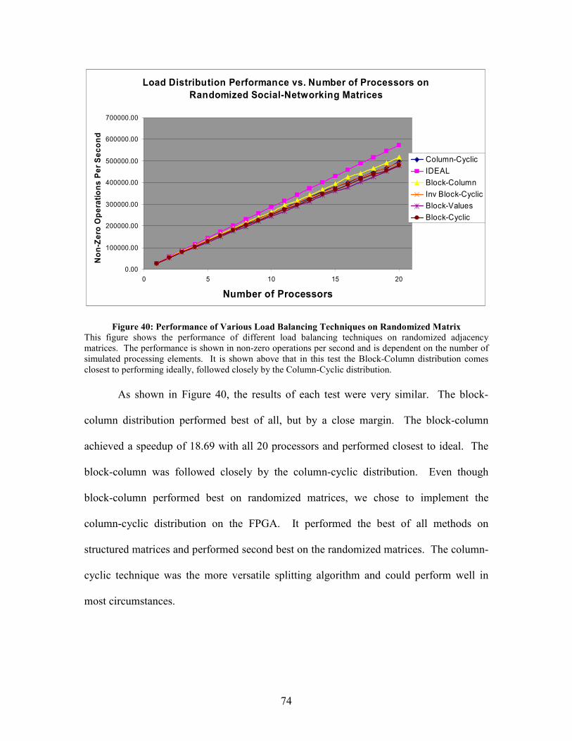
74
Load Distribution Performance vs. Number of Processors on
Randomized Social-Networking Matrices
0.00
100000.00
200000.00
300000.00
400000.00
500000.00
600000.00
700000.00
0 5 10 15 20
Number of Processors
Non-Zero Operations Per Second
Column-Cyclic
IDEAL
Block-Column
Inv Block-Cyclic
Block-Values
Block-Cyclic
Figure 40: Performance of Various Load Balancing Techniques on Randomized Matrix
This figure shows the performance of different load balancing techniques on randomized adjacency
matrices. The performance is shown in non-zero operations per second and is dependent on the number of
simulated processing elements. It is shown above that in this test the Block-Column distribution comes
closest to performing ideally, followed closely by the Column-Cyclic distribution.
As shown in Figure 40, the results of each test were very similar. The block-
column distribution performed best of all, but by a close margin. The block-column
achieved a speedup of 18.69 with all 20 processors and performed closest to ideal. The
block-column was followed closely by the column-cyclic distribution. Even though
block-column performed best on randomized matrices, we chose to implement the
column-cyclic distribution on the FPGA. It performed the best of all methods on
structured matrices and performed second best on the randomized matrices. The column-
cyclic technique was the more versatile splitting algorithm and could perform well in
most circumstances.
75
4 FPGA Implementation
Once the best algorithms for multiplication and parallelization had been decided,
the complete system was implemented on the FPGA. In the FPGA implementation, the
matrix multiplication algorithm was performed by multiple embedded Microblaze soft-
core processors working in parallel. Also, the processes of load distribution,
multiplication, and final matrix assembly were all performed by a host Microblaze which
distributed jobs to the multipliers. The optimized methods for multiplication and
parallelization were converted from functions in MATLAB to functions in the
programming language C to run on the Microblaze processors.
In the C-code implementation of these algorithms, we originally thought it would
be beneficial to develop a structure to store the sparse matrices in. We soon realized that
a C-structure to store these matrices in was not beneficial. Referencing of structures in C
reduced the efficiency of the code significantly. Instead, all of our matrix functions take
in each individual piece of information on the matrices. This means the matrix’s
dimensions, its value vector, its index vector, and its length vector are all passed in to
each function as parameters.
4.1.1 Microblaze Multiplication
It was shown previously in the Algorithm Performance Analysis section how
CRSxCCS multiplication, with each format utilizing a length vector, was the most
efficient method we tested to perform sparse matrix multiplication. The results from
these tests were why CRSxCCS multiplication was chosen for implementation on the
FPGA. To make the Microblaze processors perform this algorithm, we needed to convert
76
our previously developed code from MATLAB into C, a lower level programming
language.
4.1.1.1 C Code for CRSxCCS Multiplication
The first step to writing our parallel matrix multiplication algorithm was to
implement the CRSxCCS multiplication function in C. This code was very similar to the
MATLAB code developed previously, but it could run on the Microblaze soft-core
processor inside the FPGA. The full C-code can be found in Appendix D.
4.1.2 Parallel Microblaze Load Distribution
The chosen load distribution technique for implementation on the FPGA was the
column-cyclic distribution. This splitting algorithm was performed by software on the
Microblaze processor to split load of the matrix multiplication as evenly as possible
between the processing elements. After the multiplication had completed, the same
Microblaze reassembled the individual submatrices of C into the final matrix.
4.1.2.1 Inter-Microblaze Communication via the Fast Simplex Link
Before implementation of the splitting algorithm, communication needed to be
established between the different elements inside the FPGA. This communication was
supported through the use of the Fast Simplex Link (FSL). Configuring the FSL to
transmit data between Microblazes required modifications to the hardware configuration
file. The entire hardware configuration file, a Xilinx .mhs file, can be seen in Appendix
F.
Once the FSL hardware was configured, creating a link between two processors,
the use of the communication links was coded inside a C program. The header file fsl.h
77
must be included; and the sending and receiving of data between Microblazes is done by
using the functions putfsl(val,id) and getfsl(val,id), respectively. The function putfsl is
used by the sending processor. The function is given two parameters, the data to send
over the link and the id number of the FSL (a number 0-7) to send it through. Once the
sending processor has put the value on the FSL, getfsl must be called by the receiving
processor. The function getfsl takes in the value from the first processor and stores it in a
variable with the name given by “val”. By using these functions, data transfer between
two Microblaze processors is achieved. Each Microblaze is able to utilize up to eight Fast
Simplex Links for sending data, and another eight for receiving data.
4.1.2.2 FPGA Implementation of Column-Cyclic Distribution
Because the column-cyclic load distribution was the chosen method to implement
on the FPGA, C-code needed to be developed to split up matrix B and to reassemble the
submatrices of matrix C. The functions columnCyclic and assembleColumnCyclic are
functions that break up and reassemble the matrices, respectively. The actual C-code for
this implementation can be found in Appendix E.
78
5 Algorithm Performance Results
Once our optimized matrix multiplication algorithm had been developed using C-
code, we were able to test its efficiency against full matrix multiplication to confirm our
performance estimates and to optimize the code. The code testing and optimization of
our algorithm was more easily performed on a desktop computer. The testing against a
full matrix multiplication was completed to ensure that our algorithm worked faster,
solidifying the results obtained in MATLAB.
Once our final C-code was loaded onto the FPGA, results were obtained about the
memory usage of the soft-core microprocessors and the Fast Simplex Links. The
memory measurements were used as part of a small study of the total memory usage
inside the FPGA. Because memory space on an FPGA is often a limiting factor, the size
of the code in memory made a difference in the maximum size of the matrices our design
could store and process.
Once the FPGA hardware had been generated to utilize parallel processing
elements, tests were run with various numbers of processing elements on the FPGA to
evaluate their performance and determine the parallel speedup. A plot was generated
showing the parallel speedup factor given by an increasing number of parallel processors.
The performance of each case was measured in non-zero operations per second. Each of
these tests were done on randomized adjacency matrices with 1% density generated by
the RMAT function.
79
5.1 CRSxCCS Multiplication vs. Full Matrix Multiplication in C
In the methods section we discussed the compressed row times compressed column
multiplication method. It was shown in MATLAB that the compressed multiplication
performed much more efficiently than the full matrix multiplication. We wanted to
confirm these results by running the code on a desktop computer to be sure that this
difference in efficiency was also reflected when completed in C-code. The CRSxCCS
multiplication algorithm was tested against a full matrix multiplication function in C.
The actual C-code for the full matrix multiplication is shown in Appendix G. These tests
were run by multiplying two 128x128 adjacency matrices with 1% density together on a
PC-based Pentium 4 processor while timing the result. Our OperationsCounter function
determined that there were 412 non-zero operations required to multiply the two
matrices. The clock rate of the desktop’s processor was 3.4GHz. The processor
computed the product of the two matrices using both multiplication functions and the
total time for each was measured. The efficiency was calculated using the following
formula, as discussed in the introduction:
%100#
% ×××
=processorsrequencyOperatingFTotalTime
tionsnzeroOperaNumberofNoEfficiency
The multiplication of the two matrices was looped 10,000 times in the code to
ensure accurate measurements. To multiply the two matrices in a full matrix format, the
multiplication took 92.057 seconds. Because it performed 412x10000 non-zero
operations total, the processor performed multiplications at a rate of 44,754 non-zero
operations per second. Dividing this performance by the clock frequency (3.4 GHz)
gives an efficiency of 0.0013%.
80
The CRSxCCS multiplication performed the same loop of 4.12 million total non-
zero operations in 1.87 seconds meaning it multiplied the matrices at a rate of 2.193
Million non-zero operations per second. Dividing by the clock rate gives an efficiency of
0.0645%. From these results, we concluded that the CRSxCCS multiplication method
truly performs more efficiently; completing 49 times the non-zero operations per second
of a full matrix multiplication.
5.2 Theoretical Maximum Allowable Matrix Size
We generated a plot showing the estimated size of the matrices that the FPGA
could process vs. the number of Microblazes implemented on the Xilinx Virtex-II Pro
XC2VP30. As the number of Microblaze processing elements on the FPGA increases,
the RAM space with which to store the matrices decreases. An estimate was desired to
determine if the maximum number of parallel processors, eight, would be capable of
multiplying two of our 128x128 test matrices. A set of equations, derived subsequently,
was developed to show the trade-off between the number of processing elements and the
allowable matrix size. This prediction incorporated the size of the machine code and
Microblazes in block RAM as well as the predicted size of the resultant matrix of this
multiplication.
Through our program files in Xilinx Platform Studio 9.1, we determined that the
host processor and its instruction code, responsible for breaking up matrix B and
reassembling the final matrix, would need approximately 15.8KB of block RAM. Also,
each individual parallel Microblaze multiplier would require 12.3KB of RAM. Both of
these sizes were rounded up to 16KB.
81
To estimate how much block RAM would be available to store the matrices, we
needed to determine when and where each matrix, A, B, and C, would need to be stored
on the FPGA. Because matrix A was distributed as a whole to the individual processing
elements, every processor, including the host, needed enough memory to store matrix A.
This storage scheme meant the total memory size used for matrix A storage would be
equal to the number of processors on the FPGA times the size of a single matrix A in
memory. Matrix B would be stored on the host processor, and then an equal sized piece
of matrix B would be distributed to each parallel processor meaning that the total size
needed for matrix B would be two times the size of a single matrix B. A submatrix of the
resultant matrix C would also need to be stored in each multiplier as well as an entire
matrix C on the host processor. In an actual implementation on the FPGA, both the
splitting and rebuilding algorithms will be performed on the host processor. Because the
host processor does not need to store matrix A or B after it has sent each of them out to
the parallel processors, this space was reused to store part of matrix C.
Sparse matrix multiplications often result in a denser product matrix. Because of
this increase in density, tests were run in MATLAB to predict the density of the output
matrix. These tests were run to find the average product matrix for the multiplication of
two randomized adjacency matrices and two structured adjacency matrices. Each of
these tests utilized two adjacency matrices with dimensions 128x128 and 1% density.
The results showed that the multiplication of two randomized adjacency matrices would
result in a 128x128 matrix with average density of 1.2% and standard deviation of 0.22%.
In the case of the structured adjacency matrices, the resultant matrix would have an
average density of 3.2% with a standard deviation of 0.21%. Assuming that these matrix
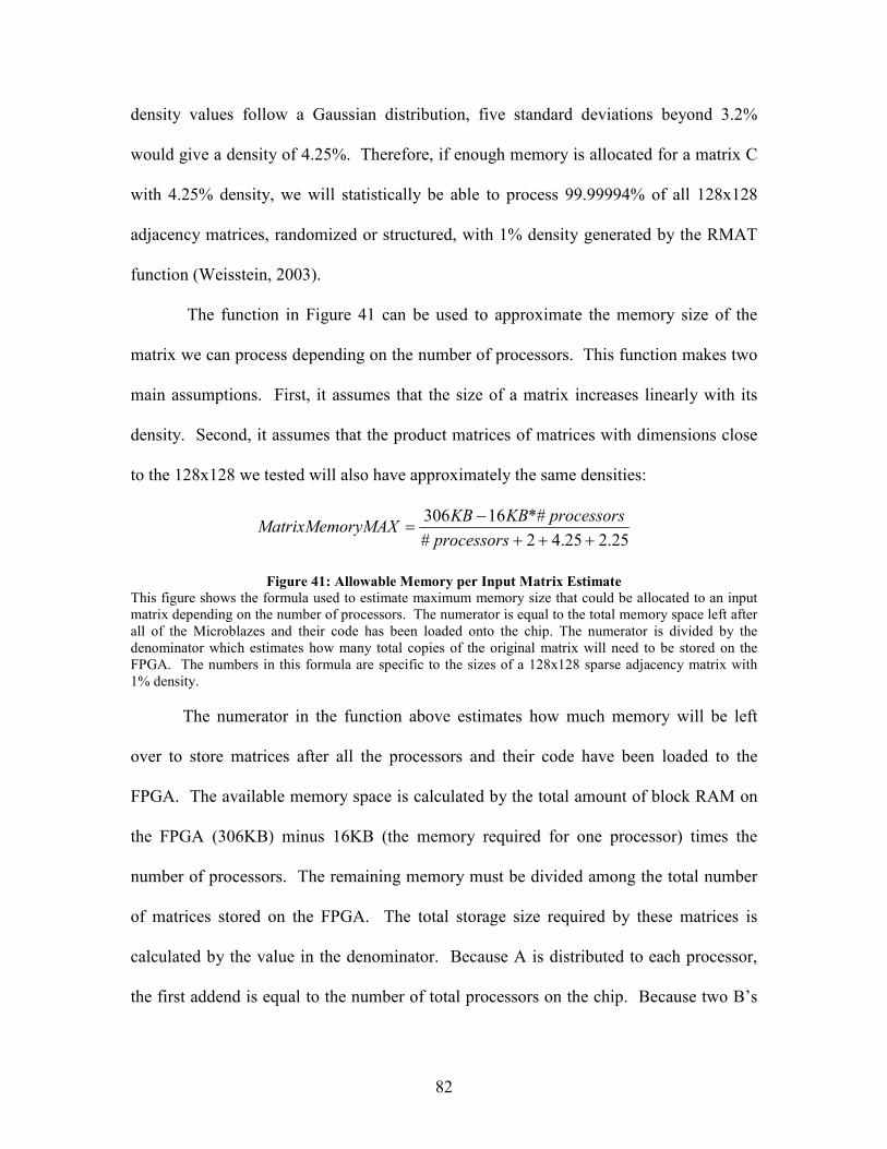
82
density values follow a Gaussian distribution, five standard deviations beyond 3.2%
would give a density of 4.25%. Therefore, if enough memory is allocated for a matrix C
with 4.25% density, we will statistically be able to process 99.99994% of all 128x128
adjacency matrices, randomized or structured, with 1% density generated by the RMAT
function (Weisstein, 2003).
The function in Figure 41 can be used to approximate the memory size of the
matrix we can process depending on the number of processors. This function makes two
main assumptions. First, it assumes that the size of a matrix increases linearly with its
density. Second, it assumes that the product matrices of matrices with dimensions close
to the 128x128 we tested will also have approximately the same densities:
25.225.42#
*#16306
+++
−=
processors
processorsKBKBryMAXMatrixMemo
Figure 41: Allowable Memory per Input Matrix Estimate
This figure shows the formula used to estimate maximum memory size that could be allocated to an input
matrix depending on the number of processors. The numerator is equal to the total memory space left after
all of the Microblazes and their code has been loaded onto the chip. The numerator is divided by the
denominator which estimates how many total copies of the original matrix will need to be stored on the
FPGA. The numbers in this formula are specific to the sizes of a 128x128 sparse adjacency matrix with
1% density.
The numerator in the function above estimates how much memory will be left
over to store matrices after all the processors and their code have been loaded to the
FPGA. The available memory space is calculated by the total amount of block RAM on
the FPGA (306KB) minus 16KB (the memory required for one processor) times the
number of processors. The remaining memory must be divided among the total number
of matrices stored on the FPGA. The total storage size required by these matrices is
calculated by the value in the denominator. Because A is distributed to each processor,
the first addend is equal to the number of total processors on the chip. Because two B’s
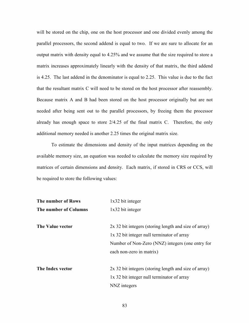
83
will be stored on the chip, one on the host processor and one divided evenly among the
parallel processors, the second addend is equal to two. If we are sure to allocate for an
output matrix with density equal to 4.25% and we assume that the size required to store a
matrix increases approximately linearly with the density of that matrix, the third addend
is 4.25. The last addend in the denominator is equal to 2.25. This value is due to the fact
that the resultant matrix C will need to be stored on the host processor after reassembly.
Because matrix A and B had been stored on the host processor originally but are not
needed after being sent out to the parallel processors, by freeing them the processor
already has enough space to store 2/4.25 of the final matrix C. Therefore, the only
additional memory needed is another 2.25 times the original matrix size.
To estimate the dimensions and density of the input matrices depending on the
available memory size, an equation was needed to calculate the memory size required by
matrices of certain dimensions and density. Each matrix, if stored in CRS or CCS, will
be required to store the following values:
The number of Rows 1x32 bit integer
The number of Columns 1x32 bit integer
The Value vector 2x 32 bit integers (storing length and size of array)
1x 32 bit integer null terminator of array
Number of Non-Zero (NNZ) integers (one entry for
each non-zero in matrix)
The Index vector 2x 32 bit integers (storing length and size of array)
1x 32 bit integer null terminator of array
NNZ integers
84
The Length vector 2x 32 bit integers (storing length and size of array)
1x 32 bit integer null terminator of array
(Row or Col integers) one for each length or row in
matrix (depending if it is CRS or CCS)
Because each compressed sparse matrix stores all of these numbers, the total size of the
matrix in memory is equal to:
KB
bytes
zerosnonrowsorofcolumnsbytes
KBinSizeMatrix
1024
int))(2)__(#11(int
4
___
−++=
Figure 42: Required Memory Space of Compressed Matrix
The equation above shows how the total memory requirements for a matrix are calculated. Each matrix
requires a number of integers to be stored in memory. There are eleven single integers plus three arrays of
integers. Two of these arrays are equal to the number of non-zero entries in the matrix. The third array is
equal to the number of columns in a column compressed matrix or the number of rows in a row compressed
matrix. All of these integers use four bytes of memory.
The equation shown in Figure 42 for matrix memory prediction was used to create
a Microsoft Excel spreadsheet which allowed a user to look up the size of a matrix by
entering the density and dimensions. The spreadsheet was used for quick reference when
determining the memory space required for square matrices of varying sizes and
densities. A sample of this spreadsheet for matrices with 1% density can be found in
Appendix H.
From these equations, the following plot was constructed to estimate the
relationship between the number of processors on the FPGA and the maximum
dimension of the square, 1% density matrices which it could process.
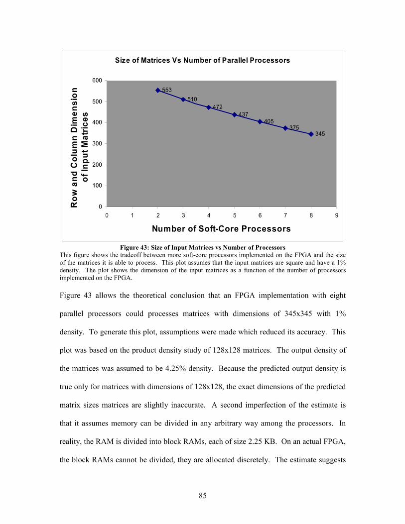
85
Size of Matrices Vs Number of Parallel Processors
553
510
472
437405
375345
0
100
200
300
400
500
600
0 1 2 3 4 5 6 7 8 9
Number of Soft-Core Processors
Row and Column Dimension
of Input Matrices
Figure 43: Size of Input Matrices vs Number of Processors
This figure shows the tradeoff between more soft-core processors implemented on the FPGA and the size
of the matrices it is able to process. This plot assumes that the input matrices are square and have a 1%
density. The plot shows the dimension of the input matrices as a function of the number of processors
implemented on the FPGA.
Figure 43 allows the theoretical conclusion that an FPGA implementation with eight
parallel processors could processes matrices with dimensions of 345x345 with 1%
density. To generate this plot, assumptions were made which reduced its accuracy. This
plot was based on the product density study of 128x128 matrices. The output density of
the matrices was assumed to be 4.25% density. Because the predicted output density is
true only for matrices with dimensions of 128x128, the exact dimensions of the predicted
matrix sizes matrices are slightly inaccurate. A second imperfection of the estimate is
that it assumes memory can be divided in any arbitrary way among the processors. In
reality, the RAM is divided into block RAMs, each of size 2.25 KB. On an actual FPGA,
the block RAMs cannot be divided, they are allocated discretely. The estimate suggests
86
that a theoretical implementation of eight parallel processors would have enough RAM
available to multiply two 128x128 matrices of 1% density.
5.3 FPGA Parallel Speedup Predictions
Before measuring results of the parallel implementation, predictions were made on
the performance of a single Microblaze performing the multiplication of two 128x128 1%
adjacency matrices. The same prediction model was used with the parallel architectures.
To make the prediction, information was gathered about the Microblaze’s performance
compared to that of a PC-based Pentium 4 processor. Once a ratio was found, predictions
of the Microblaze’s execution time for our splitting, multiplying, and reassembling
algorithms were made by running the functions on the PC-based Pentium 4 processor and
scaling by the performance ratio. These predictions were later compared to actual
measurements from certain FPGA implementations.
5.3.1 Microblaze Execution Speed
In order to estimate the performance of the 128x128 multiplication on the
Microblaze, simulations of our C-code for splitting, multiplying, and rebuilding matrices
were completed on desktop computers. First, a ratio was needed between the speed of a
Pentium 4’s execution of our algorithms and that of the Microblaze. To find this ratio, a
sample multiplication task was performed on each and timed. Our two test matrices,
128x128 with 1% density, were multiplied together. To compute the product of these
two matrices, 412 non-zero operations were required. By looping this multiplication 100
thousand times and finding its execution time on both the Pentium 4 and the Microblaze,
we were able to find a ratio between the two different processor’s performances.
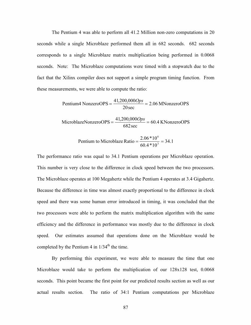
87
The Pentium 4 was able to perform all 41.2 Million non-zero computations in 20
seconds while a single Microblaze performed them all in 682 seconds. 682 seconds
corresponds to a single Microblaze matrix multiplication being performed in 0.0068
seconds. Note: The Microblaze computations were timed with a stopwatch due to the
fact that the Xilinx compiler does not support a simple program timing function. From
these measurements, we were able to compute the ratio:
SMNonzeroOP 06.2sec20
000,200,41NonzeroOPS Pentium4 ==
Ops
SKNonzeroOP 4.60sec682
000,200,41NonzeroOPSMicroblaze ==
Ops
1.3410*4.60
10*06.2Ratio Microblaze toPentium
3
6
==
The performance ratio was equal to 34.1 Pentium operations per Microblaze operation.
This number is very close to the difference in clock speed between the two processors.
The Microblaze operates at 100 Megahertz while the Pentium 4 operates at 3.4 Gigahertz.
Because the difference in time was almost exactly proportional to the difference in clock
speed and there was some human error introduced in timing, it was concluded that the
two processors were able to perform the matrix multiplication algorithm with the same
efficiency and the difference in performance was mostly due to the difference in clock
speed. Our estimates assumed that operations done on the Microblaze would be
completed by the Pentium 4 in 1/34th the time.
By performing this experiment, we were able to measure the time that one
Microblaze would take to perform the multiplication of our 128x128 test, 0.0068
seconds. This point became the first point for our predicted results section as well as our
actual results section. The ratio of 34:1 Pentium computations per Microblaze
88
computation was used to predict the matrix splitting, matrix multiplication, and matrix
rebuilding times for Microblaze systems involving parallel processors.
5.3.2 Fast Simplex Link
In the methods section, MATLAB simulations served to model the performance
gains made by parallel multiplication of matrices. These MATLAB simulations were
successful in modeling the total processing time to perform the computations, but
assumed ideal communication between processors. This communication time must be
considered when predicting multiplication in a parallel manner.
In the parallel FPGA design, the communication was between processors through
the utilization of the Fast Simplex Link. To model this performance, calculations needed
to be done involving the speed of the FSL. The FSL is a 32 bit wide bus used for fast
transfer of data between IP cores on an FPGA. The FSL is capable of transmitting 32 bits
in one clock cycle of the Microblaze, meaning that if the Microblaze runs at 100MHz, the
FSL can transmit at 400MB per second. The peak data rate of 400MB per second was
used to estimate the communication times in our performance prediction.
The imperfection in our estimates was that our FSL communications did not run
at full speed. In the case of our matrices, which are stored in vector formats, the
Microblaze must cycle through each vector and send each entry in the vector through the
FSL individually. Because of this cycling, there are extra clock cycles involved in the
sending over the FSL and the link will not perform at its top speed.
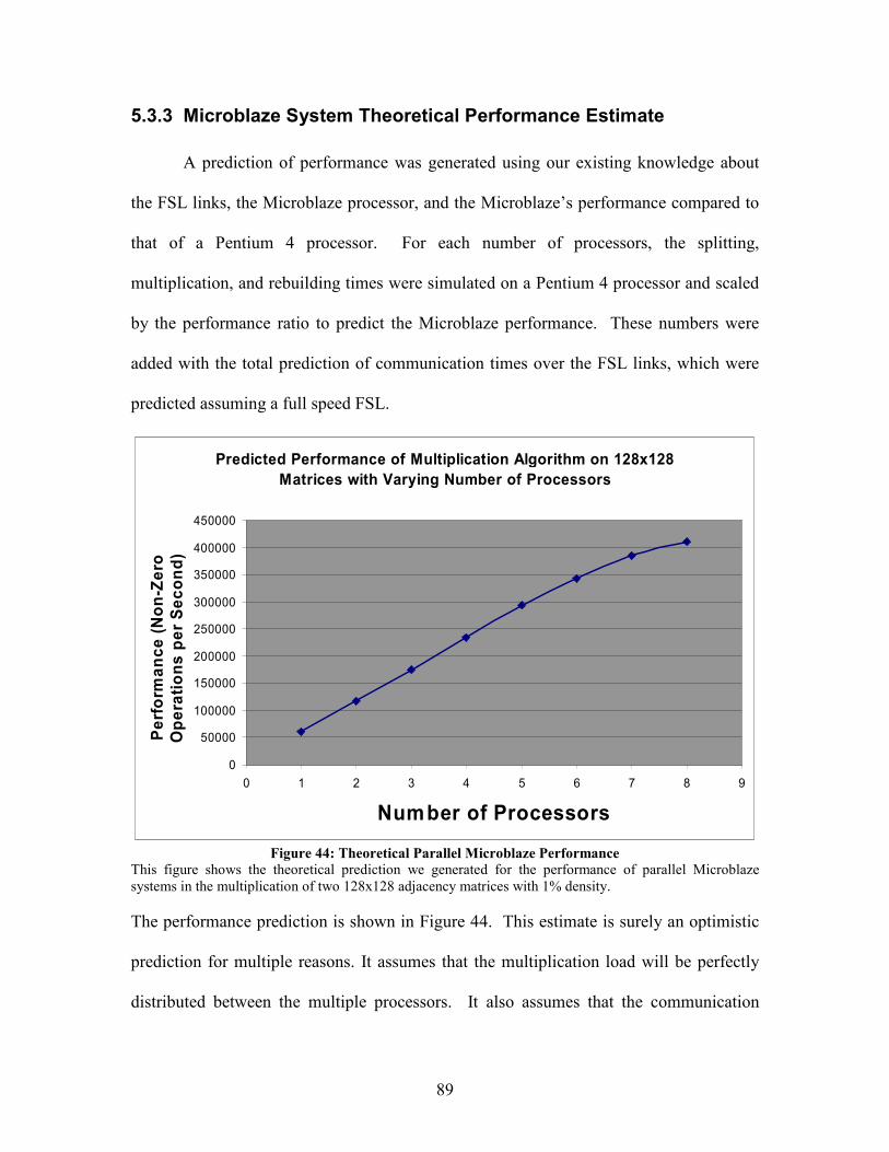
89
5.3.3 Microblaze System Theoretical Performance Estimate
A prediction of performance was generated using our existing knowledge about
the FSL links, the Microblaze processor, and the Microblaze’s performance compared to
that of a Pentium 4 processor. For each number of processors, the splitting,
multiplication, and rebuilding times were simulated on a Pentium 4 processor and scaled
by the performance ratio to predict the Microblaze performance. These numbers were
added with the total prediction of communication times over the FSL links, which were
predicted assuming a full speed FSL.
Predicted Performance of Multiplication Algorithm on 128x128
Matrices with Varying Number of Processors
0
50000
100000
150000
200000
250000
300000
350000
400000
450000
0 1 2 3 4 5 6 7 8 9
Number of Processors
Performance (Non-Zero
Operations per Second)
Figure 44: Theoretical Parallel Microblaze Performance
This figure shows the theoretical prediction we generated for the performance of parallel Microblaze
systems in the multiplication of two 128x128 adjacency matrices with 1% density.
The performance prediction is shown in Figure 44. This estimate is surely an optimistic
prediction for multiple reasons. It assumes that the multiplication load will be perfectly
distributed between the multiple processors. It also assumes that the communication
90
between the Microblazes will work at its full speed, 400MB per second. The real
multiplication load will not be perfectly distributed between the Microblaze processing
elements and the FSL, as discussed previously, needs to cycle through the entries in each
vector meaning that data transfer will not happen at its full speed. The measured
performance curve will level off more quickly as more processors are added. This
estimate served as prediction for the actual performance of parallel Microblaze systems.
After actual implementation of parallel Microblazes, the measured performance was
compared against the prediction from Figure 44.
5.4 FPGA Parallel Speedup Measurements
Two separate hardware configurations were successfully implemented and tested
on the FPGA. The first system was a single Microblaze system used as a benchmark to
show the difference in performance between one processor and parallel processors. The
second system implemented was a system with three Microblaze processors; a host
processor and two Microblazes connected to work in parallel. The host processor
performed the splitting algorithm on matrix B and the reassembly algorithm on the
submatrices of matrix C. Figure 45 shows the block diagram of the parallel configuration
of two Microblazes.
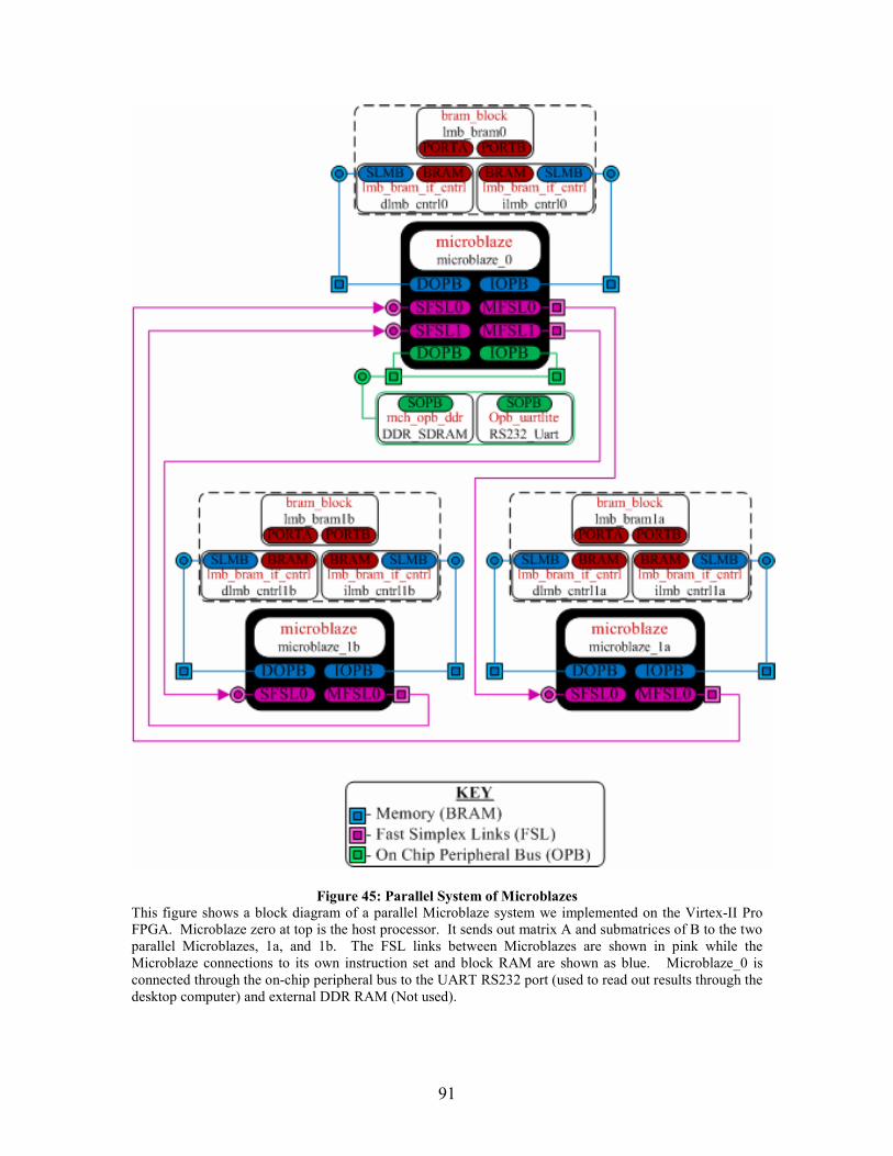
91
Figure 45: Parallel System of Microblazes
This figure shows a block diagram of a parallel Microblaze system we implemented on the Virtex-II Pro
FPGA. Microblaze zero at top is the host processor. It sends out matrix A and submatrices of B to the two
parallel Microblazes, 1a, and 1b. The FSL links between Microblazes are shown in pink while the
Microblaze connections to its own instruction set and block RAM are shown as blue. Microblaze_0 is
connected through the on-chip peripheral bus to the UART RS232 port (used to read out results through the
desktop computer) and external DDR RAM (Not used).
92
The hardware configuration (.mhs) files for both the single Microblaze system and the
parallel Microblaze system can be found in Appendix F. The hardware configuration
files are used by the Xilinx compiler to configure hardware on the FPGA.
Multiple implementations of parallel architectures such as three, four, or even eight
processors in parallel were outside the scope of this project. A single implementation of
two processors in parallel was all that was needed to simulate the performance of more
parallel processors. The final results for both one Microblaze and two parallel
Microblazes are actual results, while all implementations with more than two parallel
processors were simulated on the two processor implementation and compiled to predict
performances for more parallel Microblazes. The performances of parallel
implementations were calculated using the following formula, as discussed in the
introduction:
TotalTime
rationsNonzeroOpeePerformanc =
Once we implemented a parallel architecture consisting of one host Microblaze and
two parallel Microblazes, measurements were taken to determine the parallel speedup
possible with this architecture. To measure the actual performance, the code was run on
the Microblaze and timed. Because we could not directly measure the performance of
other parallel implementations, these results were simulated using the existing parallel
implementation on the FPGA. Each communication, multiplication, and splitting process
that would happen in larger parallel implementations was simulated using the two
Microblazes system and timed, allowing us to measure performance of further
parallelized systems.
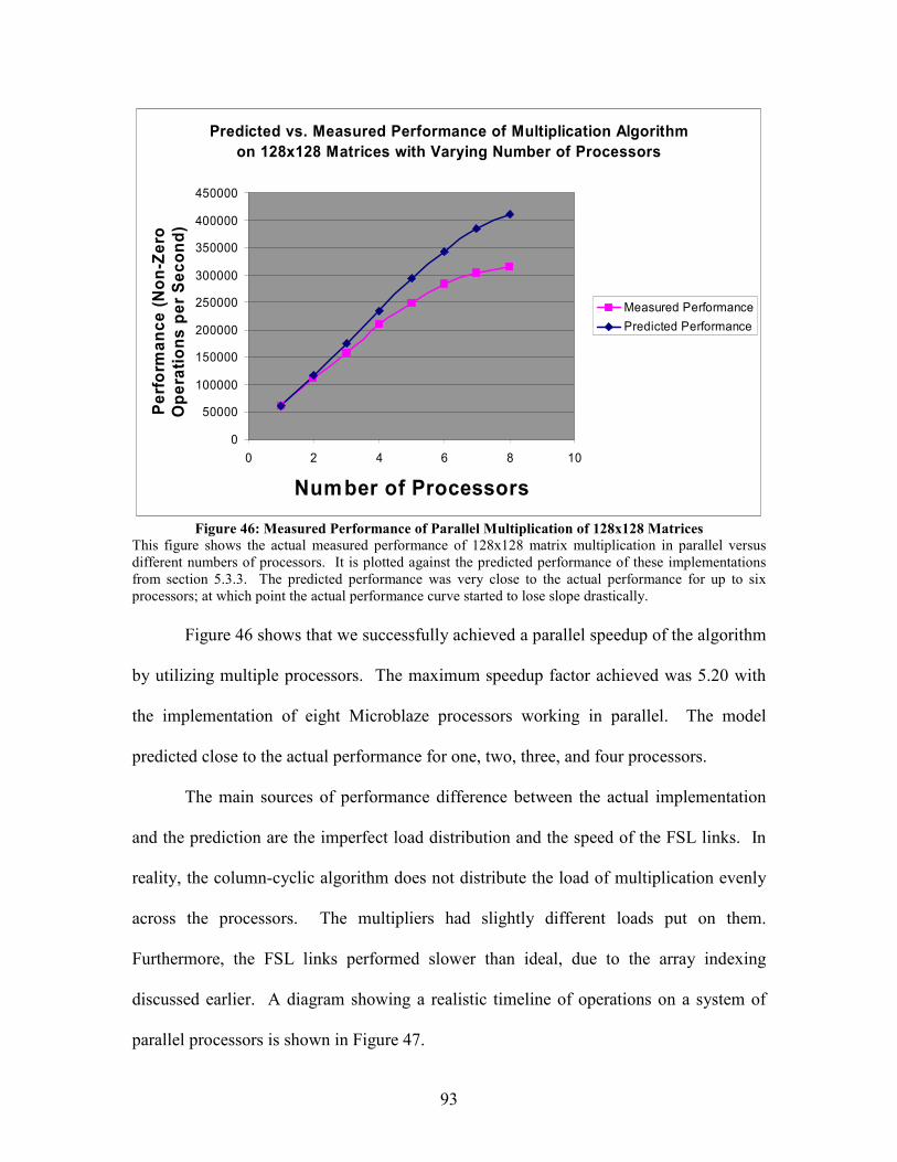
93
Predicted vs. Measured Performance of Multiplication Algorithm
on 128x128 Matrices with Varying Number of Processors
0
50000
100000
150000
200000
250000
300000
350000
400000
450000
0 2 4 6 8 10
Number of Processors
Performance (Non-Zero
Operations per Second)
Measured Performance
Predicted Performance
Figure 46: Measured Performance of Parallel Multiplication of 128x128 Matrices
This figure shows the actual measured performance of 128x128 matrix multiplication in parallel versus
different numbers of processors. It is plotted against the predicted performance of these implementations
from section 5.3.3. The predicted performance was very close to the actual performance for up to six
processors; at which point the actual performance curve started to lose slope drastically.
Figure 46 shows that we successfully achieved a parallel speedup of the algorithm
by utilizing multiple processors. The maximum speedup factor achieved was 5.20 with
the implementation of eight Microblaze processors working in parallel. The model
predicted close to the actual performance for one, two, three, and four processors.
The main sources of performance difference between the actual implementation
and the prediction are the imperfect load distribution and the speed of the FSL links. In
reality, the column-cyclic algorithm does not distribute the load of multiplication evenly
across the processors. The multipliers had slightly different loads put on them.
Furthermore, the FSL links performed slower than ideal, due to the array indexing
discussed earlier. A diagram showing a realistic timeline of operations on a system of
parallel processors is shown in Figure 47.
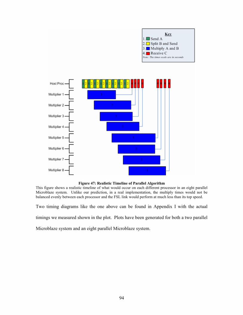
94
Figure 47: Realistic Timeline of Parallel Algorithm
This figure shows a realistic timeline of what would occur on each different processor in an eight parallel
Microblaze system. Unlike our prediction, in a real implementation, the multiply times would not be
balanced evenly between each processor and the FSL link would perform at much less than its top speed.
Two timing diagrams like the one above can be found in Appendix I with the actual
timings we measured shown in the plot. Plots have been generated for both a two parallel
Microblaze system and an eight parallel Microblaze system.
95
6 Discussion and Conclusions
We were successful in developing a highly efficient and parallelizable algorithm
for the multiplication of two sparse matrices. Furthermore, we were able to display a
performance increase in this algorithm by mapping it over multiple parallel processors.
6.1 Sparse Matrix Multiplication Algorithm
Our first goal was as follows:
To determine a highly parallelizable method for the storage and multiplication of
two sparsely populated matrices which can perform computations at efficiencies
comparable to the 0.05% to 0.1% achieved by optimized sparse matrix
multiplications on traditional microprocessor systems.
Our optimized method for storage and multiplication was to store matrix A in a
row-compressed format and matrix B in a column-compressed format. Each of these
matrices was stored using the length vector. The multiplication algorithm performed
vector by vector multiplication, multiplying a row of matrix A by a column of matrix B at
a time. Because of the row and column compressed formats, the values in the same row
of matrix A and the same column of matrix B were stored locally. This type of data
locality proved to be the optimal storage method among the methods we tested to perform
matrix multiplication.
When operating on our test matrices, randomized adjacency matrices with
dimensions of 128x128 and densities of 1%, our algorithm for multiplication achieved an
efficiency of 0.0645% on a PC-based Pentium 4 processor when implemented using C-
code. This efficiency means that our algorithm is comparable to the efficiencies of
96
between 0.05 and 0.1% achieved by the most optimized sparse matrix multiplication
algorithms today while our algorithm also maintains high parallelizability. Our algorithm
performs at about 49 times the efficiency of a full matrix multiplication (0.0013%
efficiency) when processing a sparsely populated matrix.
6.2 Parallelization of Multiplication Algorithm on FPGA
The second goal of our project, as stated in the introduction, was as follows:
To demonstrate how the optimized multiplication algorithm can be
parallelized on a single FPGA to achieve a parallel speedup by
distributing the load over multiple processing elements.
This goal was achieved as discussed in section Error! Reference source not found..
We were able to measure a parallel speedup of 5.20 through the implementation of eight
Microblazes in parallel.
The parallelization technique we used distributed the entire matrix A to every
parallel processor. Assuming that N is the total number of parallel processors, Matrix B
was distributed using a column-cyclic splitting algorithm which split it into N
submatrices each containing approximately 1/N of the total columns in B. The splitting
algorithm was performed by the host processor. Each parallel processor multiplied
matrix A times its submatrix of B and output a submatrix of the final matrix, matrix C, in
a column compressed format. The pieces of matrix C in column compressed format were
put through a reassembly algorithm which constructed the final matrix. This type of
parallelization technique is useful information to researchers at Lincoln Laboratory as
well as other scientists or engineers who are interested in the parallelizing of sparse
matrix multiplication.
97
6.3 Future Recommendations
We have determined promising paths for further research into parallel sparse matrix
multiplication on an FPGA. Implementation of these ideas may be able to further
increase the effectiveness of similar FPGA designs. These ideas include new methods for
transferring data between the system’s components, a lower level type of multiplication
algorithm, and the implementation of specialized, gate-level logic circuits to complete the
compressed sparse matrix multiplication.
A major consumer of time in our FPGA design was the communication between
system components. The FSL required serial transmission of data from one processor to
another. An improvement that may help speed up the transfer of data is sharing of the
same RAM between processors. With the freedom involved in FPGA design, if an
engineer could implement the sharing of RAM among multiple processors, the parallel
processors could begin multiplication immediately after the splitting algorithm had been
performed by the host. The communication times in this type of design would be reduced
significantly because the parallel processors would only have to access memory, not
receive serial transmissions.
A second recommendation is to implement a bitwise method to search for
intersecting indices in a row and column. The compressed row by compressed column
multiplication algorithm currently indexes through the corresponding indices given by a
row of A and a column of B searching for common entries in the two vectors. These
indices could be mapped, bit by bit, into a small memory buffer to easily find
intersections. For example, if there was an entry in column five of the row vector and
row five of the column vector, a one would be written to the fifth bit of each buffer
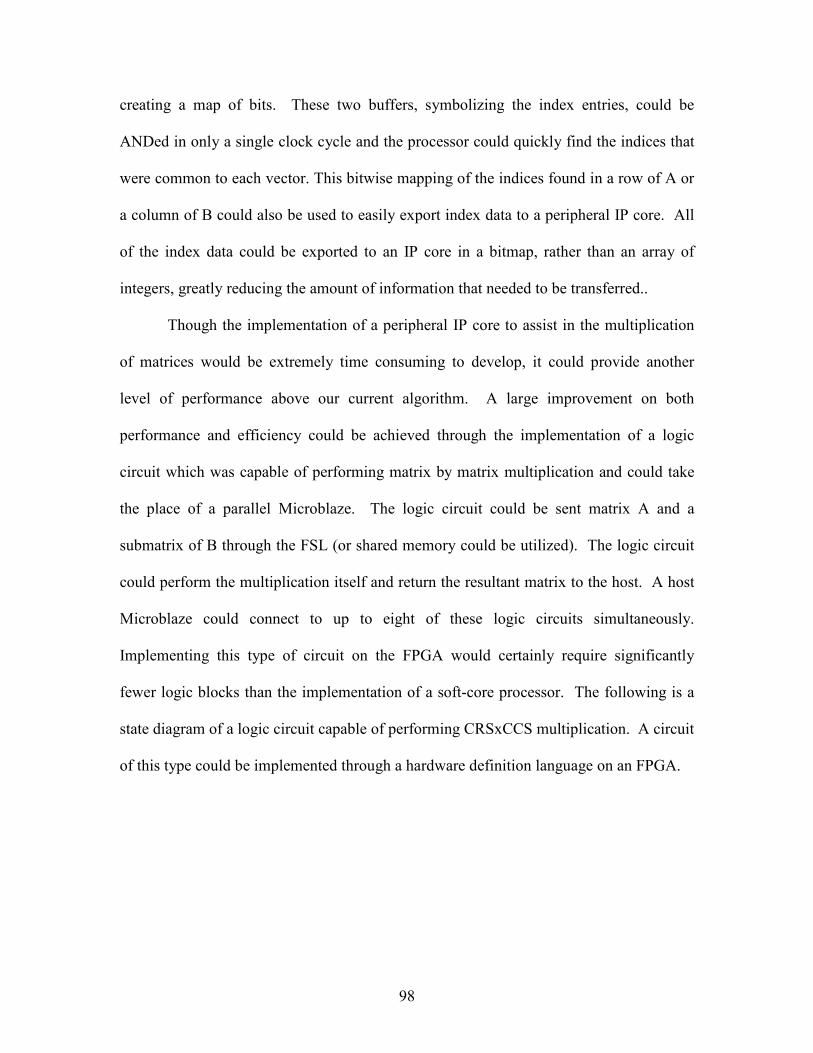
98
creating a map of bits. These two buffers, symbolizing the index entries, could be
ANDed in only a single clock cycle and the processor could quickly find the indices that
were common to each vector. This bitwise mapping of the indices found in a row of A or
a column of B could also be used to easily export index data to a peripheral IP core. All
of the index data could be exported to an IP core in a bitmap, rather than an array of
integers, greatly reducing the amount of information that needed to be transferred..
Though the implementation of a peripheral IP core to assist in the multiplication
of matrices would be extremely time consuming to develop, it could provide another
level of performance above our current algorithm. A large improvement on both
performance and efficiency could be achieved through the implementation of a logic
circuit which was capable of performing matrix by matrix multiplication and could take
the place of a parallel Microblaze. The logic circuit could be sent matrix A and a
submatrix of B through the FSL (or shared memory could be utilized). The logic circuit
could perform the multiplication itself and return the resultant matrix to the host. A host
Microblaze could connect to up to eight of these logic circuits simultaneously.
Implementing this type of circuit on the FPGA would certainly require significantly
fewer logic blocks than the implementation of a soft-core processor. The following is a
state diagram of a logic circuit capable of performing CRSxCCS multiplication. A circuit
of this type could be implemented through a hardware definition language on an FPGA.
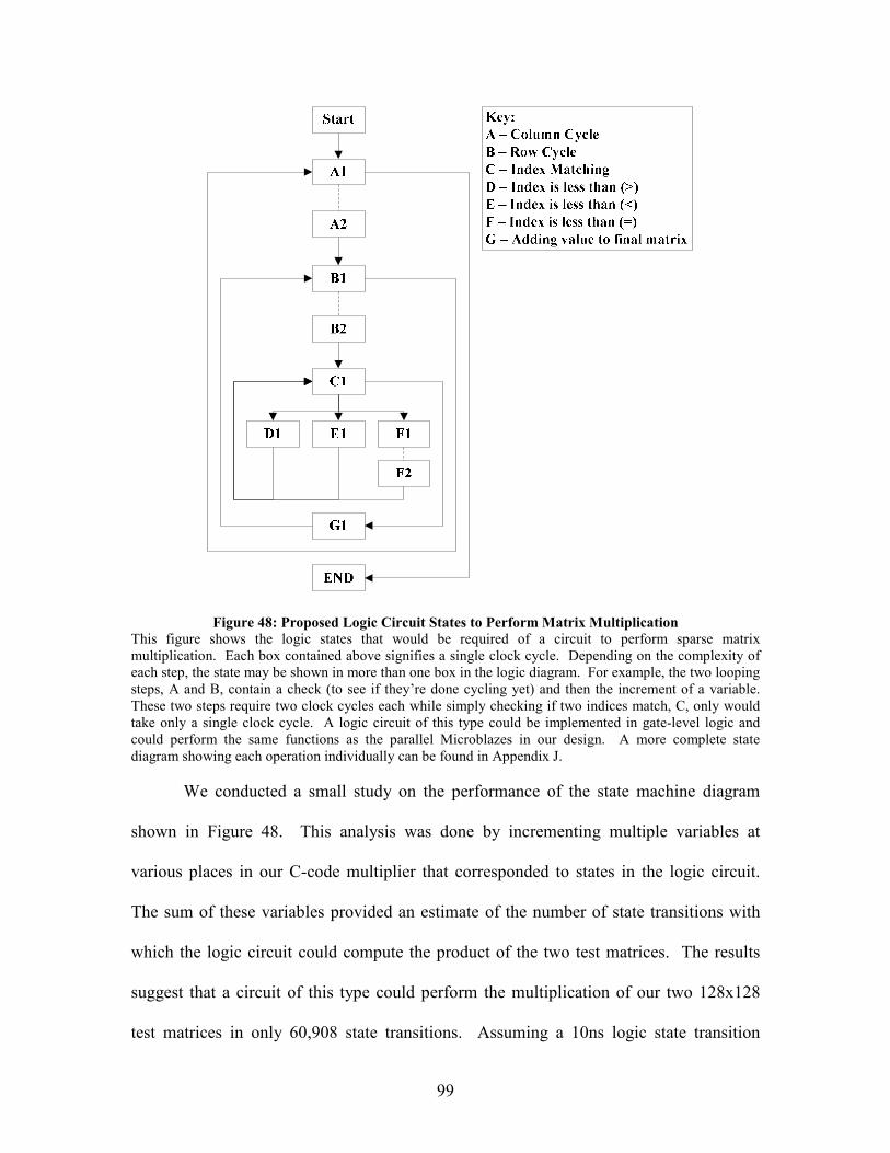
99
Figure 48: Proposed Logic Circuit States to Perform Matrix Multiplication
This figure shows the logic states that would be required of a circuit to perform sparse matrix
multiplication. Each box contained above signifies a single clock cycle. Depending on the complexity of
each step, the state may be shown in more than one box in the logic diagram. For example, the two looping
steps, A and B, contain a check (to see if they’re done cycling yet) and then the increment of a variable.
These two steps require two clock cycles each while simply checking if two indices match, C, only would
take only a single clock cycle. A logic circuit of this type could be implemented in gate-level logic and
could perform the same functions as the parallel Microblazes in our design. A more complete state
diagram showing each operation individually can be found in Appendix J.
We conducted a small study on the performance of the state machine diagram
shown in Figure 48. This analysis was done by incrementing multiple variables at
various places in our C-code multiplier that corresponded to states in the logic circuit.
The sum of these variables provided an estimate of the number of state transitions with
which the logic circuit could compute the product of the two test matrices. The results
suggest that a circuit of this type could perform the multiplication of our two 128x128
test matrices in only 60,908 state transitions. Assuming a 10ns logic state transition
100
period (equal to the Microblaze’s clock cycle of 100MHz), 60,908 state transitions
corresponds to a total computation time of 610 microseconds, 11 times faster than the 6.8
ms of which the C algorithm run on a Microblaze is capable.
With different combinations of hardware circuits and soft-core processors, an
FPGA system’s performance could increase the performance of our implementation
hundreds of times over as shown in Figure 49.
# Microblazes Only C
Algorithm
1 Logic Circuit
Per Processor
4 Logic Circuits
Per Processor
8 Logic Circuits
Per Processor
1 Microblaze 1 11.16 44.65 89.32
4 Microblaze 3.57 39.84 159.4 318.9
8 Microblaze 5.20 58.03 232.2 464.5
Figure 49: Projected Speedups with Microblazes and Logic Circuits
This figure shows the theoretical speedup factors that could be attained over the current abilities with a
single Microblaze. The speedups with multiple Microblazes were obtained from the data we collected in
our parallel experiments. The speedups given by the implementation of logic circuits are optimistic
predictions based on the state transition counts for the logic state machine shown in Figure 48.
Implementation of some of these recommendations could help to develop an
FPGA with performance and efficiency far beyond those we achieved in this project.
Sparse matrix multiplication is an extremely difficult problem for a computer engineer
and more time and research into parallel architectures, advanced algorithms, and logic
circuits for performing these multiplications need to be done before these matrices can be
processed effectively.
6.4 Future Impacts
The research we have performed into parallelizable sparse matrix multiplication
will have many future impacts for research MIT Lincoln Laboratory. Because of the high
level research we have performed, results from our project can filter down to many
101
different types of systems for sparse matrix processing. Results of our project could
assist researchers with sparse matrix processing on multi-core processors, logic circuit
implementations, or even grid computing.
The value in this project comes from the methods for storage of sparse matrices and
parallelizable multiplication we developed. Our implementation of multiple processor
cores on a single FPGA was not faster than even a single Pentium 4, but the algorithm
and parallelization method can be replicated in other systems that could potentially
perform multiplication hundreds of times faster than even the fastest desktop computer as
shown in Figure 50.
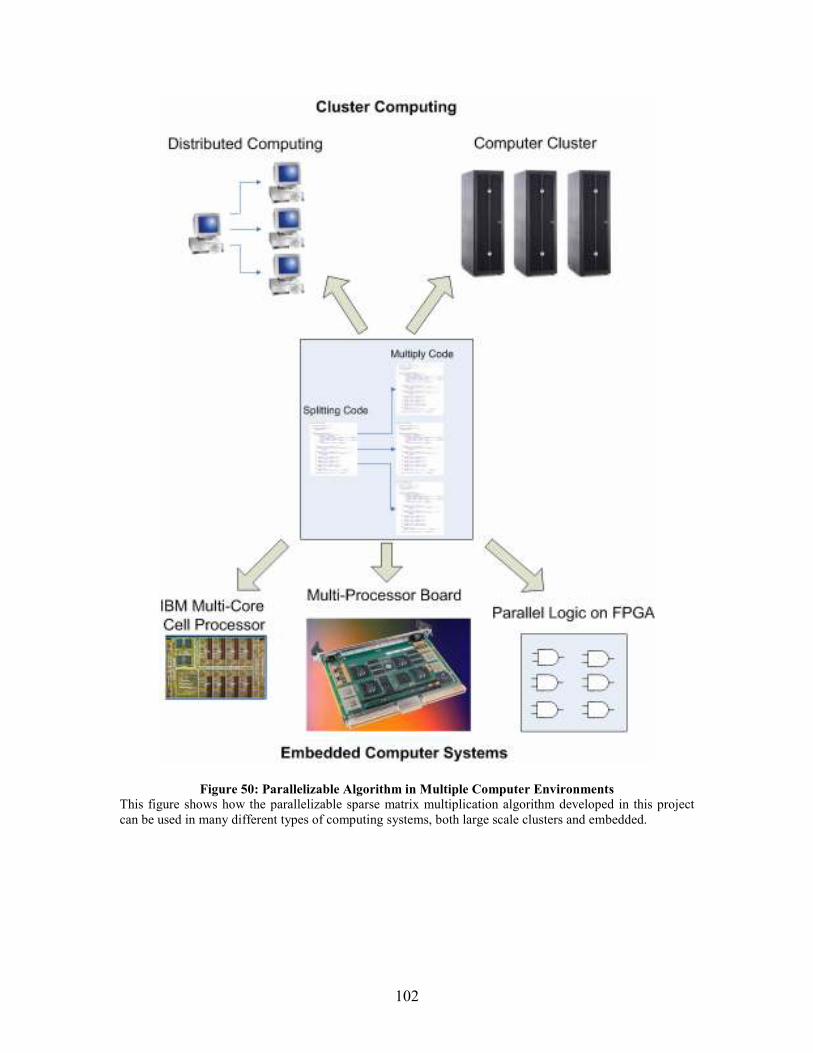
102
Figure 50: Parallelizable Algorithm in Multiple Computer Environments
This figure shows how the parallelizable sparse matrix multiplication algorithm developed in this project
can be used in many different types of computing systems, both large scale clusters and embedded.

103
Annotated Reference List
Bliss, Nadya T. E-Mail interview. 20 Sept. 2007. These numbers are based on
information taken off of figures sent to us by Nadya Bliss on the performance of
sparse and full matrix multiplications on a 1.5 GHz PowerPC microprocessor and
a 3.2 GHz Intel Xeon Processor.
Borgatti, Stephen P. The Key Player Problem. Dynamic Social Network Modeling and
Analysis, 2002, National Research Council of the National Academies.
Washington, DC: National Academies P, 2002. A research paper presented at a
workshop on social network analysis in 2002. The workshop was sponsored by
National Research Council committee on Human Factors. The paper focuses on
finding the key people in any social network.
Chen, Danny Z., comp. Developing Algorithms and Software for Geometric Path
Planning Problems. University of Notre Dame, Department of Computer Science.
Sept. 2007. <http://www.cs.brown.edu/people/rt/sdcr/chen/chen.html>. A student
website which discusses the importance of developing algorithms to find the
shortest path between vertices in a graph.
Cofer, R. C., and Ben Harding. Rapid System Prototyping with FPGAs: Accelerating the
Design Process. Burlington, MA: Elsevier, 2006. A text book discussing the
rapid development of embedded systems using FPGAs.
Davis, Timothy, comp. University of Florida Sparse Matrix Collection. University of
Florida. June-July 2007.
<http://www.cise.ufl.edu/research/sparse/matrices/index.html>. A large
collection of sparse matrices and information on sparse matrices compiled by Tim
Davis, an Associate Professor at the University of Florida.
104
Dongarra, J., comp. Sparse Matrix Storage Formats. University of Tennessee At
Knoxville. June-July 2007.
<http://www.cs.utk.edu/~dongarra/etemplates/node372.html>. An online version
of a book on sparse matrices by J. Dongarra. It is found on a website maintained
by the University of Tennessee at Knoxville. It discusses various methods of
compressing sparse matrices depending on their structures.
Eskowitz, Michael, Vitaliy Gleyzer, James Haupt, and Roya Mirhosseini. Adaptive
Beamforming Using Field Programmable Gate Array Embedded
Microprocessors. Worcester Polytechnic Institute Major Qualifying Project.
Worcester, Ma, 2004. A Major Qualifying Project report by former students at
Worcester Polytechnic Institute. It discusses the use of soft-core microprocessors
embedded on FPGAs to develop an embedded system used for adaptive
beamforming applications.
Floyd, Thomas. Digital Fundamentals. Upper Saddle River, NJ: Pearson/Prentice Hall,
2006. 642. A basic textbook on the fundamentals of digital logic design.
Groww, Jonathan L., and Jay Yellen. Handbook of Graph Theory. CRC P, 2004. 2. A
popular book on graph theory. It discusses algorithms to pull important
information out of graphs as well as the many applications of graph theory.
Holme, Petter, Beom Jun Kim, Chang No Yoon, and Seung Kee Han. Attack
Vulnerability of Complex Networks. American Physical Society. 2002. Aug.-
Sept. 2007. <http://prola.aps.org/pdf/PRE/v65/i5/e056109>. A research paper
discussing the disassembly of complex networks by the removal of the most
important vertices.
Leskovec, Jure, and Christos Faloutsos. Scalable Modeling of Real Graphs Using
Kronecker Multiplication. Carnegie Mellon University. International Conference
105
on Machine Learning, 2007. 20 Sept. 2007.
<http://www.cs.cmu.edu/~jure/pubs/kronFit-icml07.pdf>. A research paper
discussing the use of Kronecker Graphs to simulate realistic graphs.
ML310 User Guide. Xilinx Inc. Xilinx Inc., 2007. 1 Oct. 2007.
<http://direct.xilinx.com/bvdocs/userguides/ug068.pdf>. The users guide for
Xilinx's ML310 Embedded Development Platform.
Oldfield, John V., and Richard C. Dorf. Field Programmable Gate Arrays. New York:
John Wiley and Sons Inc., 1995. xvi. A book discussing the advantages of using
FPGAs in the development of embedded systems.
Pellerin, David, and Scott Thibault. Practical FPGA Programming in C. Westford, MA:
Prentice Hall, 2007. 27. A book describing the use of C-Programming to develop
FPGA solutions for embedded systems design.
Robinson, Eric. "Array Based Betweenness Centrality." MIT Lincoln Laboratory.
Summer Intern Presentations. MIT Lincoln Laboratory, Lexington, MA. 8 Aug.
2007. A presentation given by Eric Robinson, a 2007 summer intern at Lincoln
Laboratory, on computer algorithms for betweenness centrality calculations on
large graphs.
Rosinger, Hans-Peter. Connecting Customized IP to the MicroBlaze Soft Processor Using
the Fast Simplex Link (FSL) Channel. Xilinx, Inc. 2004. Sept. 2007.
<http://www.xilinx.com/bvdocs/appnotes/xapp529.pdf>. An instructional report
found on Xilinx's website about the use of the Fast Simplex Link to speed up
connectivity between IP cores and the Xilinx Microblaze processor in embedded
system design.
"Signals Intelligence Homepage." NSA.Gov. National Security Agency. 29 Aug. 2007.
<http://www.nsa.gov/sigint/index.cfm>. A website found off the homepage of the
106
National Security Agency. It outlines the process of processing raw data to
convert it into useable information in the context of Signals Intelligence
(SIGINT).
"Virtex-II Pro / Prox PowerPC 405 Processor." Xilinx.Com. Xilinx, Inc. 10 Sept. 2007.
<http://www.xilinx.com/products/silicon_solutions/fpgas/virtex/virtex_ii_pro_fpg
as/capabilities/powerpc.htm>. A site found off of Xilinx's homepage which
discusses the capabilities of the PowerPC processor in embedded systems design
using their Virtex II pro FPGA.
Virtex-II Pro Data Sheet. Xilinx Inc. Xilinx Inc., 2005. 1 Oct. 2007.
<http://www.xilinx.com/bvdocs/publications/ds083.pdf>. A data sheet containing
data on the Xilinx Virtex-II Pro FPGAs.
Weisstein, Eric W. "Matrix Multiplication." Mathworld-a Wolfram Web Resource. 21
Mar. 2006. 24 Sept. 2007.
<http://mathworld.wolfram.com/MatrixMultiplication.html>. A webpage
discussing the intricacies of how to perform matrix multiplications. It is found on
Wolfram MathWorld, a mathematics website.
Weisstein, Eric W. "Standard Deviation." Mathworld-a Wolfram Web Resource. 17 Oct.
2003. 5 Oct. 2007. <http://mathworld.wolfram.com/StandardDeviation.html>. A
website on standard deviations. It is found on Wolfram MathWorld, a
mathematics website.
"Xilinx Microprocessor Controller and Peripheral." Xilinx.Com. Xilinx, Inc. 6 Sept.
2007.
<http://www.xilinx.com/xlnx/xebiz/designResources/ip_product_details.jsp?key=
micro_blaze>. A webpage found off of Xilinx's homepage. It discusses the use
107
of the Microblaze soft-core processor in embedded systems development using
Xilinx FPGAs.
Zhuo, Ling, and Viktor K. Prasanna. "Sparse Matrix-Vector Multiplication on FPGAs."
Proceedings of the 2005 ACM/SIGDA 13th International Symposium on Field-
Programmable Gate Arrays (2005). 1 June 2007.
<http://portal.acm.org/citation.cfm?id=1046202>. A paper presented at an FPGA
conference in 2005. It discusses the FPGA structure and circuits used to perform
compute the product of a sparse matrix times a vector.
Zlatev, Zahari. Computational Methods for General Sparse Matrices. Boston, MA:
Kluwer Academic, 1991. A book discussing the optimization of sparse matrix
processing algorithms in computer systems.
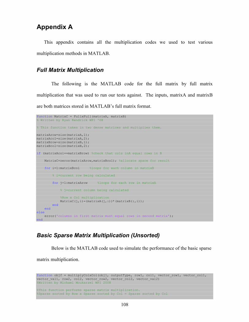
108
Appendix A
This appendix contains all the multiplication codes we used to test various
multiplication methods in MATLAB.
Full Matrix Multiplication
The following is the MATLAB code for the full matrix by full matrix
multiplication that was used to run our tests against. The inputs, matrixA and matrixB
are both matrices stored in MATLAB’s full matrix format.
function MatrixC = FullxFull(matrixA, matrixB) % Written by Ryan Kendrick WPI '08 % This function takes in two dense matrices and multiplies them. matrixArow=size(matrixA,1); matrixAcol=size(matrixA,2); matrixBrow=size(matrixB,1); matrixBcol=size(matrixB,2); if (matrixAcol==matrixBrow) %check that cols inA equal rows in B MatrixC=zeros(matrixArow,matrixBcol); %allocate space for result for i=1:matrixBcol %loops for each column in matrixB % i=current row being calculated for j=1:matrixArow %loops for each row in matrixA % j=current column being calculated %Row x Col multiplication MatrixC(j,i)=(matrixA(j,:))*(matrixB(:,i)); end end else error('columns in first matrix must equal rows in second matrix'); end
Basic Sparse Matrix Multiplication (Unsorted)
Below is the MATLAB code used to simulate the performance of the basic sparse
matrix multiplication.
function objf = multiplyColxCol(obj1, outputType, row1, col1, vector_row1, vector_col1, vector_val1, row2, col2, vector_row2, vector_col2, vector_val2) %Written by Michael Moukarzel WPI 2008 %This function performs sparse matrix multiplication. %Sparse sorted by Row x Sparse sorted by Col = Sparse sorted by Col
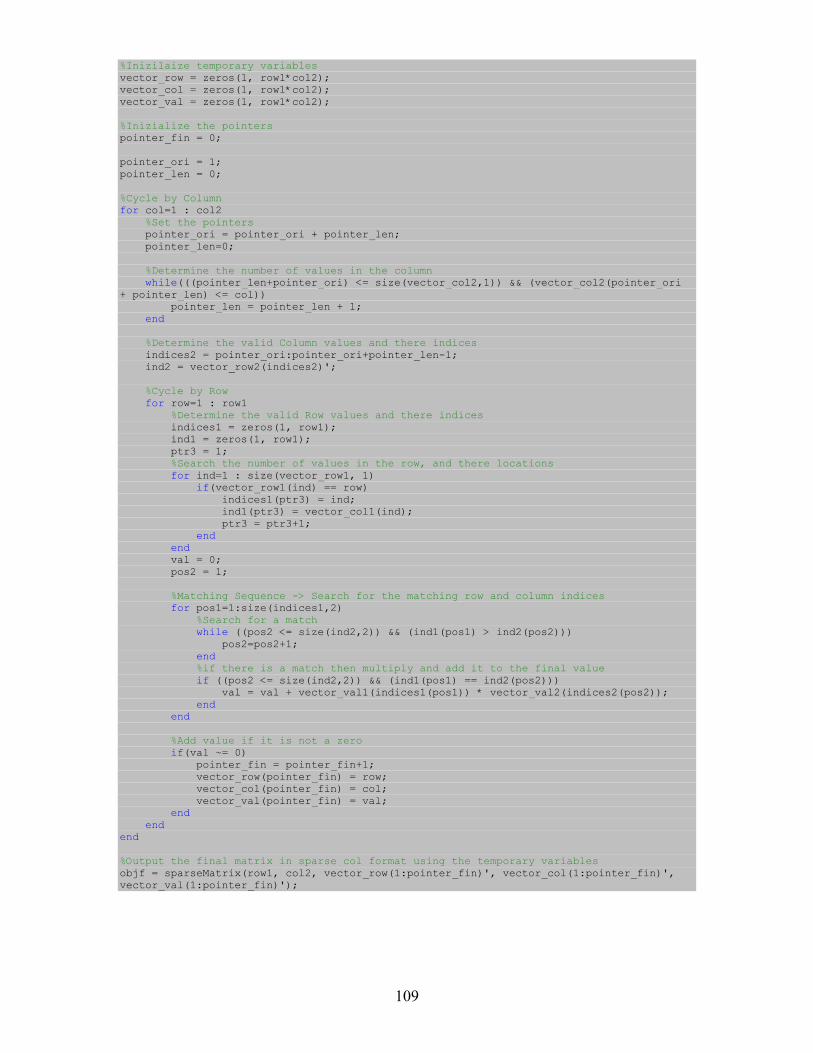
109
%Inizilaize temporary variables vector_row = zeros(1, row1*col2); vector_col = zeros(1, row1*col2); vector_val = zeros(1, row1*col2); %Inizialize the pointers pointer_fin = 0; pointer_ori = 1; pointer_len = 0; %Cycle by Column for col=1 : col2 %Set the pointers pointer_ori = pointer_ori + pointer_len; pointer_len=0; %Determine the number of values in the column while(((pointer_len+pointer_ori) <= size(vector_col2,1)) && (vector_col2(pointer_ori + pointer_len) <= col)) pointer_len = pointer_len + 1; end %Determine the valid Column values and there indices indices2 = pointer_ori:pointer_ori+pointer_len-1; ind2 = vector_row2(indices2)'; %Cycle by Row for row=1 : row1 %Determine the valid Row values and there indices indices1 = zeros(1, row1); ind1 = zeros(1, row1); ptr3 = 1; %Search the number of values in the row, and there locations for ind=1 : size(vector_row1, 1) if(vector_row1(ind) == row) indices1(ptr3) = ind; ind1(ptr3) = vector_col1(ind); ptr3 = ptr3+1; end end val = 0; pos2 = 1; %Matching Sequence -> Search for the matching row and column indices for pos1=1:size(indices1,2) %Search for a match while ((pos2 <= size(ind2,2)) && (ind1(pos1) > ind2(pos2))) pos2=pos2+1; end %if there is a match then multiply and add it to the final value if ((pos2 <= size(ind2,2)) && (ind1(pos1) == ind2(pos2))) val = val + vector_val1(indices1(pos1)) * vector_val2(indices2(pos2)); end end %Add value if it is not a zero if(val ~= 0) pointer_fin = pointer_fin+1; vector_row(pointer_fin) = row; vector_col(pointer_fin) = col; vector_val(pointer_fin) = val; end end end %Output the final matrix in sparse col format using the temporary variables objf = sparseMatrix(row1, col2, vector_row(1:pointer_fin)', vector_col(1:pointer_fin)', vector_val(1:pointer_fin)');
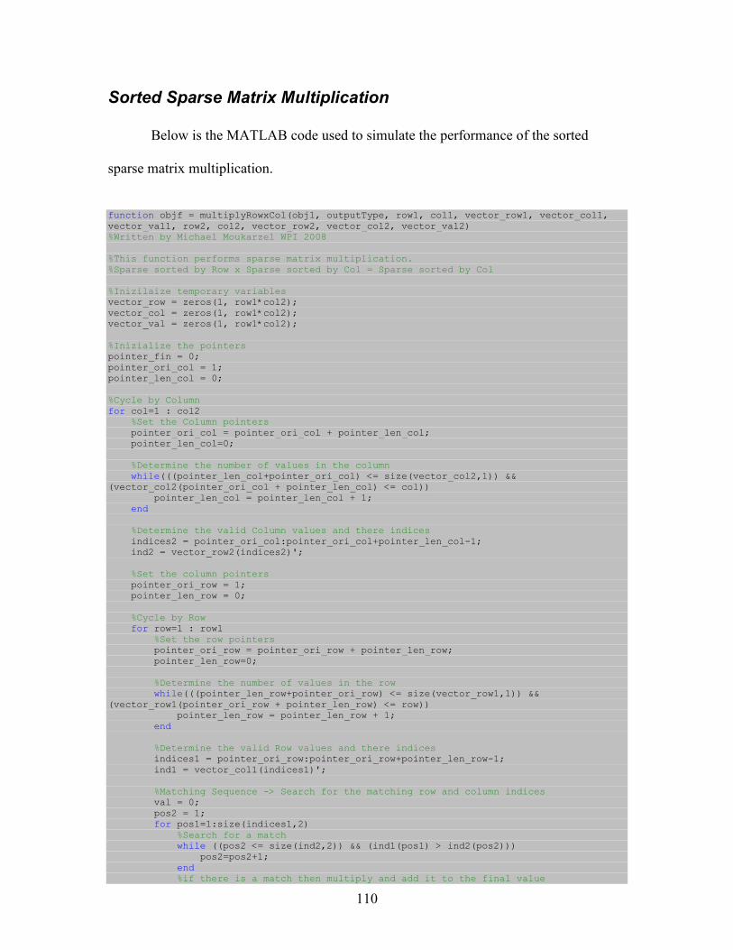
110
Sorted Sparse Matrix Multiplication
Below is the MATLAB code used to simulate the performance of the sorted
sparse matrix multiplication.
function objf = multiplyRowxCol(obj1, outputType, row1, col1, vector_row1, vector_col1, vector_val1, row2, col2, vector_row2, vector_col2, vector_val2) %Written by Michael Moukarzel WPI 2008 %This function performs sparse matrix multiplication. %Sparse sorted by Row x Sparse sorted by Col = Sparse sorted by Col %Inizilaize temporary variables vector_row = zeros(1, row1*col2); vector_col = zeros(1, row1*col2); vector_val = zeros(1, row1*col2); %Inizialize the pointers pointer_fin = 0; pointer_ori_col = 1; pointer_len_col = 0; %Cycle by Column for col=1 : col2 %Set the Column pointers pointer_ori_col = pointer_ori_col + pointer_len_col; pointer_len_col=0; %Determine the number of values in the column while(((pointer_len_col+pointer_ori_col) <= size(vector_col2,1)) && (vector_col2(pointer_ori_col + pointer_len_col) <= col)) pointer_len_col = pointer_len_col + 1; end %Determine the valid Column values and there indices indices2 = pointer_ori_col:pointer_ori_col+pointer_len_col-1; ind2 = vector_row2(indices2)'; %Set the column pointers pointer_ori_row = 1; pointer_len_row = 0; %Cycle by Row for row=1 : row1 %Set the row pointers pointer_ori_row = pointer_ori_row + pointer_len_row; pointer_len_row=0; %Determine the number of values in the row while(((pointer_len_row+pointer_ori_row) <= size(vector_row1,1)) && (vector_row1(pointer_ori_row + pointer_len_row) <= row)) pointer_len_row = pointer_len_row + 1; end %Determine the valid Row values and there indices indices1 = pointer_ori_row:pointer_ori_row+pointer_len_row-1; ind1 = vector_col1(indices1)'; %Matching Sequence -> Search for the matching row and column indices val = 0; pos2 = 1; for pos1=1:size(indices1,2) %Search for a match while ((pos2 <= size(ind2,2)) && (ind1(pos1) > ind2(pos2))) pos2=pos2+1; end %if there is a match then multiply and add it to the final value
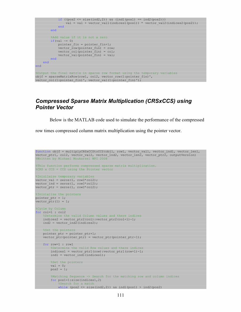
111
if ((pos2 <= size(ind2,2)) && (ind1(pos1) == ind2(pos2))) val = val + vector_val1(indices1(pos1)) * vector_val2(indices2(pos2)); end end %Add value if it is not a zero if(val ~= 0) pointer_fin = pointer_fin+1; vector_row(pointer_fin) = row; vector_col(pointer_fin) = col; vector_val(pointer_fin) = val; end end end %Output the final matrix in sparse row format using the temporary variables objf = sparseMatrixRow(row1, col2, vector_row(1:pointer_fin)', vector_col(1:pointer_fin)', vector_val(1:pointer_fin)');
Compressed Sparse Matrix Multiplication (CRSxCCS) using Pointer Vector
Below is the MATLAB code used to simulate the performance of the compressed
row times compressed column matrix multiplication using the pointer vector.
function objf = multiplyCRSxCCStoCCS(obj1, row1, vector_val1, vector_ind1, vector_len1, vector_ptr1, col2, vector_val2, vector_ind2, vector_len2, vector_ptr2, outputVersion) %Written by Michael Moukarzel WPI 2008 %This function performs compressed sparse matrix multiplication. %CRS x CCS = CCS using the Pointer vector %Inizilaize temporary variables vector_val = zeros(1, row1*col2); vector_ind = zeros(1, row1*col2); vector_ptr = zeros(1, row1*col2); %Inizialize the pointers pointer_ptr = 1; vector_ptr(1) = 1; %Cycle by Column for col=1 : col2 %Determine the valid Column values and there indices indices2 = vector_ptr2(col):vector_ptr2(col+1)-1; ind2 = vector_ind2(indices2); %Set the pointers pointer_ptr = pointer_ptr+1; vector_ptr(pointer_ptr) = vector_ptr(pointer_ptr-1); for row=1 : row1 %Determine the valid Row values and there indices indices1 = vector_ptr1(row):vector_ptr1(row+1)-1; ind1 = vector_ind1(indices1); %Set the pointers val = 0; pos2 = 1; %Matching Sequence -> Search for the matching row and column indices for pos1=1:size(indices1,2) %Search for a match while (pos2 <= size(ind2,2)) && ind1(pos1) > ind2(pos2)
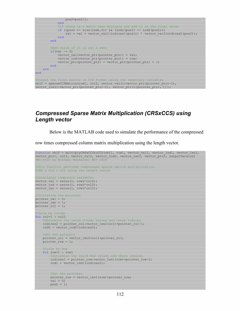
112
pos2=pos2+1; end %if there is a match then multiply and add it to the final value if ((pos2 <= size(ind2,2)) && (ind1(pos1) == ind2(pos2))) val = val + vector_val1(indices1(pos1)) * vector_val2(indices2(pos2)); end end %Add value if it is not a zero if(val ~= 0) vector_val(vector_ptr(pointer_ptr)) = val; vector_ind(vector_ptr(pointer_ptr)) = row; vector_ptr(pointer_ptr) = vector_ptr(pointer_ptr) + 1; end end end %Output the final matrix in CCS format using the temporary variables objf = sparseCCSMatrix(row1, col2, vector_val(1:vector_ptr(pointer_ptr)-1), vector_ind(1:vector_ptr(pointer_ptr)-1), vector_ptr(1:pointer_ptr), []);
Compressed Sparse Matrix Multiplication (CRSxCCS) using Length vector
Below is the MATLAB code used to simulate the performance of the compressed
row times compressed column matrix multiplication using the length vector.
function objf = multiplyCRSxCCStoCCS(obj1, row1, vector_val1, vector_ind1, vector_len1, vector_ptr1, col2, vector_val2, vector_ind2, vector_len2, vector_ptr2, outputVersion) %Written by Michael Moukarzel WPI 2008 %This function performs compressed sparse matrix multiplication. %CRS x CCS = CCS using the Length vector %Inizilaize temporary variables vector_val = zeros(1, row1*col2); vector_ind = zeros(1, row1*col2); vector_len = zeros(1, row1*col2); %Inizialize the pointers pointer_val = 0; pointer_len = 1; pointer_col = 1; %Cycle by Column for col=1 : col2 %Determine the valid Column values and there indices indices2 = pointer_col:vector_len2(col)+pointer_col-1; ind2 = vector_ind2(indices2); %Set the pointers pointer_col = vector_len2(col)+pointer_col; pointer_row = 1; %Cycle by Row for row=1 : row1 %Determine the valid Row values and there indices indices1 = pointer_row:vector_len1(row)+pointer_row-1; ind1 = vector_ind1(indices1); %Set the pointers pointer_row = vector_len1(row)+pointer_row; val = 0; pos2 = 1;
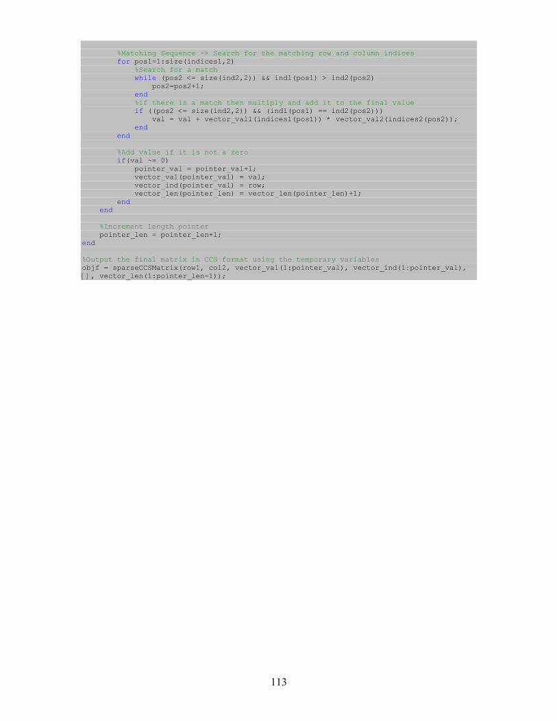
113
%Matching Sequence -> Search for the matching row and column indices for pos1=1:size(indices1,2) %Search for a match while (pos2 <= size(ind2,2)) && ind1(pos1) > ind2(pos2) pos2=pos2+1; end %if there is a match then multiply and add it to the final value if ((pos2 <= size(ind2,2)) && (ind1(pos1) == ind2(pos2))) val = val + vector_val1(indices1(pos1)) * vector_val2(indices2(pos2)); end end %Add value if it is not a zero if(val ~= 0) pointer_val = pointer_val+1; vector_val(pointer_val) = val; vector_ind(pointer_val) = row; vector_len(pointer_len) = vector_len(pointer_len)+1; end end %Increment length pointer pointer_len = pointer_len+1; end %Output the final matrix in CCS format using the temporary variables objf = sparseCCSMatrix(row1, col2, vector_val(1:pointer_val), vector_ind(1:pointer_val), [], vector_len(1:pointer_len-1));
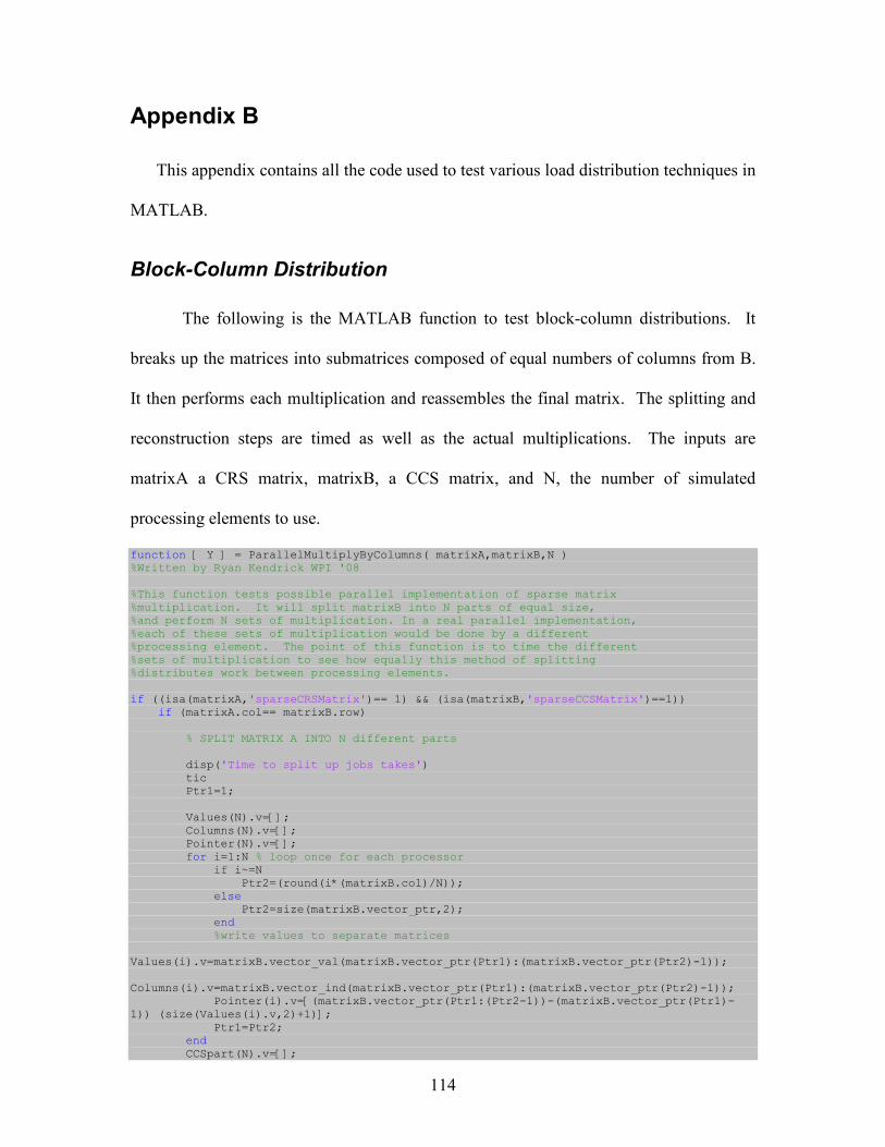
114
Appendix B
This appendix contains all the code used to test various load distribution techniques in
MATLAB.
Block-Column Distribution
The following is the MATLAB function to test block-column distributions. It
breaks up the matrices into submatrices composed of equal numbers of columns from B.
It then performs each multiplication and reassembles the final matrix. The splitting and
reconstruction steps are timed as well as the actual multiplications. The inputs are
matrixA a CRS matrix, matrixB, a CCS matrix, and N, the number of simulated
processing elements to use.
function [ Y ] = ParallelMultiplyByColumns( matrixA,matrixB,N ) %Written by Ryan Kendrick WPI '08 %This function tests possible parallel implementation of sparse matrix %multiplication. It will split matrixB into N parts of equal size, %and perform N sets of multiplication. In a real parallel implementation, %each of these sets of multiplication would be done by a different %processing element. The point of this function is to time the different %sets of multiplication to see how equally this method of splitting %distributes work between processing elements. if ((isa(matrixA,'sparseCRSMatrix')== 1) && (isa(matrixB,'sparseCCSMatrix')==1)) if (matrixA.col== matrixB.row) % SPLIT MATRIX A INTO N different parts disp('Time to split up jobs takes') tic Ptr1=1; Values(N).v=[]; Columns(N).v=[]; Pointer(N).v=[]; for i=1:N % loop once for each processor if i~=N Ptr2=(round(i*(matrixB.col)/N)); else Ptr2=size(matrixB.vector_ptr,2); end %write values to separate matrices Values(i).v=matrixB.vector_val(matrixB.vector_ptr(Ptr1):(matrixB.vector_ptr(Ptr2)-1)); Columns(i).v=matrixB.vector_ind(matrixB.vector_ptr(Ptr1):(matrixB.vector_ptr(Ptr2)-1)); Pointer(i).v=[(matrixB.vector_ptr(Ptr1:(Ptr2-1))-(matrixB.vector_ptr(Ptr1)-1)) (size(Values(i).v,2)+1)]; Ptr1=Ptr2; end CCSpart(N).v=[];
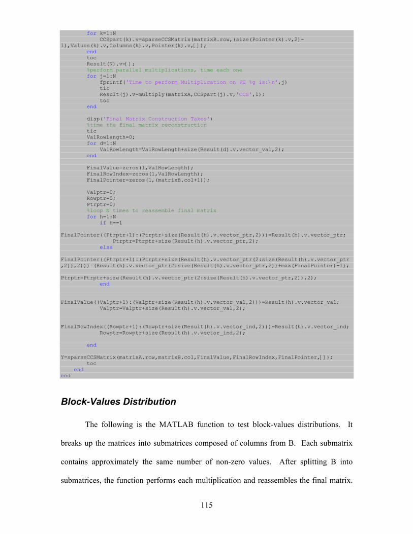
115
for k=1:N CCSpart(k).v=sparseCCSMatrix(matrixB.row,(size(Pointer(k).v,2)-1),Values(k).v,Columns(k).v,Pointer(k).v,[]); end toc Result(N).v=[]; %perform parallel multiplications, time each one for j=1:N fprintf('Time to perform Multiplication on PE %g is:\n',j) tic Result(j).v=multiply(matrixA,CCSpart(j).v,'CCS',1); toc end disp('Final Matrix Construction Takes') %time the final matrix reconstruction tic ValRowLength=0; for d=1:N ValRowLength=ValRowLength+size(Result(d).v.vector_val,2); end FinalValue=zeros(1,ValRowLength); FinalRowIndex=zeros(1,ValRowLength); FinalPointer=zeros(1,(matrixB.col+1)); Valptr=0; Rowptr=0; Ptrptr=0; %loop N times to reassemble final matrix for h=1:N if h==1 FinalPointer((Ptrptr+1):(Ptrptr+size(Result(h).v.vector_ptr,2)))=Result(h).v.vector_ptr; Ptrptr=Ptrptr+size(Result(h).v.vector_ptr,2); else FinalPointer((Ptrptr+1):(Ptrptr+size(Result(h).v.vector_ptr(2:size(Result(h).v.vector_ptr,2)),2)))=(Result(h).v.vector_ptr(2:size(Result(h).v.vector_ptr,2))+max(FinalPointer)-1); Ptrptr=Ptrptr+size(Result(h).v.vector_ptr(2:size(Result(h).v.vector_ptr,2)),2); end FinalValue((Valptr+1):(Valptr+size(Result(h).v.vector_val,2)))=Result(h).v.vector_val; Valptr=Valptr+size(Result(h).v.vector_val,2); FinalRowIndex((Rowptr+1):(Rowptr+size(Result(h).v.vector_ind,2)))=Result(h).v.vector_ind; Rowptr=Rowptr+size(Result(h).v.vector_ind,2); end Y=sparseCCSMatrix(matrixA.row,matrixB.col,FinalValue,FinalRowIndex,FinalPointer,[]); toc end end
Block-Values Distribution
The following is the MATLAB function to test block-values distributions. It
breaks up the matrices into submatrices composed of columns from B. Each submatrix
contains approximately the same number of non-zero values. After splitting B into
submatrices, the function performs each multiplication and reassembles the final matrix.
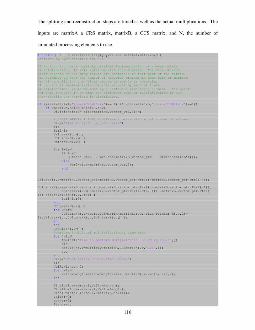
116
The splitting and reconstruction steps are timed as well as the actual multiplications. The
inputs are matrixA a CRS matrix, matrixB, a CCS matrix, and N, the number of
simulated processing elements to use.
function [ Y ] = ParallelMultiplyByValues( matrixA,matrixB,N ) %Written by Ryan Kendrick WPI '08 %This function tests possible parallel implementation of sparse matrix %multiplication. It will split matrixB into N parts. The size of each %part depends on how many values are contained in that part of the matrix. %It attempts to keep the number of nonzeros present in each part of matrixB %equal by splitting the Values vector as evenly as possible. %In an actual implementation of this algorithm, each of these %multiplications would be done by a different processing element. The point %of this function is to time the different sets of multiplication to see %how equally the workload is distributed. if ((isa(matrixA,'sparseCRSMatrix')== 1) && (isa(matrixB,'sparseCCSMatrix')==1)) if (matrixA.col== matrixB.row) DivisionsizeB= size(matrixB.vector_val,2)/N; % SPLIT MATRIX A INTO N different parts with equal number of values disp('Time to split up jobs takes') tic Ptr1=1; Values(N).v=[]; Columns(N).v=[]; Pointer(N).v=[]; for i=1:N if i~=N [trash Ptr2] = min(abs(matrixB.vector_ptr - (DivisionsizeB*i))); else Ptr2=size(matrixB.vector_ptr,2); end Values(i).v=matrixB.vector_val(matrixB.vector_ptr(Ptr1):(matrixB.vector_ptr(Ptr2)-1)); Columns(i).v=matrixB.vector_ind(matrixB.vector_ptr(Ptr1):(matrixB.vector_ptr(Ptr2)-1)); Pointer(i).v=[(matrixB.vector_ptr(Ptr1:(Ptr2-1))-(matrixB.vector_ptr(Ptr1)-1)) (size(Values(i).v,2)+1)]; Ptr1=Ptr2; end CCSpart(N).v=[]; for k=1:N CCSpart(k).v=sparseCCSMatrix(matrixB.row,(size(Pointer(k).v,2)-1),Values(k).v,Columns(k).v,Pointer(k).v,[]); end toc Result(N).v=[]; %perform individual multiplications, time each for j=1:N fprintf('Time to perform Multiplication on PE %g is:\n',j) tic Result(j).v=multiply(matrixA,CCSpart(j).v,'CCS',1); toc end disp('Final Matrix Construction Takes') tic ValRowLength=0; for d=1:N ValRowLength=ValRowLength+size(Result(d).v.vector_val,2); end FinalValue=zeros(1,ValRowLength); FinalRowIndex=zeros(1,ValRowLength); FinalPointer=zeros(1,(matrixB.col+1)); Valptr=0; Rowptr=0; Ptrptr=0;
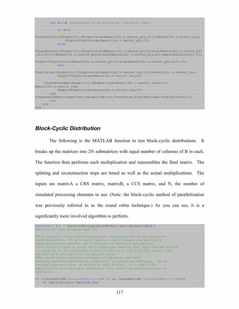
117
for h=1:N %reassemble final matrix by looping N times if h==1 FinalPointer((Ptrptr+1):(Ptrptr+size(Result(h).v.vector_ptr,2)))=Result(h).v.vector_ptr; Ptrptr=Ptrptr+size(Result(h).v.vector_ptr,2); else FinalPointer((Ptrptr+1):(Ptrptr+size(Result(h).v.vector_ptr(2:size(Result(h).v.vector_ptr,2)),2)))=(Result(h).v.vector_ptr(2:size(Result(h).v.vector_ptr,2))+max(FinalPointer)-1); Ptrptr=Ptrptr+size((Result(h).v.vector_ptr(2:size(Result(h).v.vector_ptr,2))),2); end FinalValue((Valptr+1):(Valptr+size(Result(h).v.vector_val,2)))=Result(h).v.vector_val; Valptr=Valptr+size(Result(h).v.vector_val,2); FinalRowIndex((Rowptr+1):(Rowptr+size(Result(h).v.vector_ind,2)))= Result(h).v.vector_ind; Rowptr=Rowptr+size(Result(h).v.vector_ind,2); end Y=sparseCCSMatrix(matrixA.row,matrixB.col,FinalValue,FinalRowIndex,FinalPointer,[]); toc end end
Block-Cyclic Distribution
The following is the MATLAB function to test block-cyclic distributions. It
breaks up the matrices into 2N submatrices with equal number of columns of B in each.
The function then performs each multiplication and reassembles the final matrix. The
splitting and reconstruction steps are timed as well as the actual multiplications. The
inputs are matrixA a CRS matrix, matrixB, a CCS matrix, and N, the number of
simulated processing elements to use. (Note: the block-cyclic method of parallelization
was previously referred to as the round robin technique.) As you can see, it is a
significantly more involved algorithm to perform.
function [ Y ] = ParallelMultiplyRoundRobin( matrixA,matrixB,N ) %Written by Ryan Kendrick WPI '08 %This function tests possible parallel implementation of sparse matrix %multiplication. It will split matrix B into N parts and perform N %multiplications between the N matrices of matrix B and matrixA. %This function uses a round robin technique meaning that each smaller matrix %is made up of two different pieces of matrix B, one from the denser side %of matrix B and one from the sparser side. %The round robin technique attempts to equalize the work %between separate processors; Especially in power-law matrices. The N %multiplications occur in series in this M-file...in a real life %application with multiple processors they would run simultaneously in %parallel. if ((isa(matrixA,'sparseCRSMatrix')== 1) && (isa(matrixB,'sparseCCSMatrix')==1)) if (matrixA.col== matrixB.row)
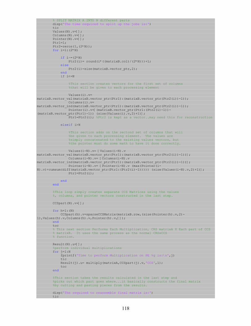
118
% SPLIT MATRIX A INTO N different parts disp('The time required to split up the jobs is:') tic Values(N).v=[]; Columns(N).v=[]; Pointer(N).v=[]; Ptr1=1; Ptr2=zeros(1,(2*N)); for i=1:(2*N) if i~=(2*N) Ptr2(i)= round(i*((matrixB.col)/(2*N)))+1; else Ptr2(i)=size(matrixB.vector_ptr,2); end if i<=N %This section creates vectors for the first set of columns %that will be given to each processing element Values(i).v= matrixB.vector_val(matrixB.vector_ptr(Ptr1):(matrixB.vector_ptr(Ptr2(i))-1)); Columns(i).v= matrixB.vector_ind(matrixB.vector_ptr(Ptr1):(matrixB.vector_ptr(Ptr2(i))-1)); Pointer(i).v=[(matrixB.vector_ptr(Ptr1:(Ptr2(i)-1))-(matrixB.vector_ptr(Ptr1)-1)) (size(Values(i).v,2)+1)]; Ptr1=Ptr2(i); %Ptr2 is kept as a vector..may need this for reconstruction elseif i>N %This section adds on the sectond set of columns that will %be given to each processing element. The values are %simply concatenated to the existing values vectors, but %the pointer must do some math to have it done correctly. Values(i-N).v= [Values(i-N).v matrixB.vector_val(matrixB.vector_ptr(Ptr1):(matrixB.vector_ptr(Ptr2(i))-1))]; Columns(i-N).v= [Columns(i-N).v matrixB.vector_ind(matrixB.vector_ptr(Ptr1):(matrixB.vector_ptr(Ptr2(i))-1))]; Pointer(i-N).v= [Pointer(i-N).v (max(Pointer(i-N).v)+cumsum(diff(matrixB.vector_ptr(Ptr1:(Ptr2(i)-1))))) (size(Values(i-N).v,2)+1)]; Ptr1=Ptr2(i); end end %This loop simply creates separate CCS Matrices using the values %, columns, and pointer vectors constructed in the last step. CCSpart(N).v=[]; for h=1:(N) CCSpart(h).v=sparseCCSMatrix(matrixB.row,(size(Pointer(h).v,2)-1),Values(h).v,Columns(h).v,Pointer(h).v,[]); end toc % This next section Performs Each Multiplication, CRS matrixA X Each part of CCS % matrixB. It uses the same process as the normal CRSxCCS % function. Result(N).u=[]; %perform individual multiplications for j=1:N fprintf('Time to perform Multiplication on PE %g is:\n',j) tic Result(j).u= multiply(matrixA,CCSpart(j).v,'CCS',1); toc end %This section takes the results calculated in the last step and %picks out which part goes where...it basically constructs the final matrix %by cutting and pasting pieces from the results. disp('The required to reassemble final matrix is:') tic
119
ColDist=[(Ptr2(1)-1) diff(Ptr2)]; %Makes a vector showing the column distriibution %How many columns each piece of B is %made up of ValRowLength=0; for d=1:N ValRowLength=ValRowLength+size(Result(d).u.vector_val,2); end FinalValue=zeros(1,ValRowLength); FinalRowIndex=zeros(1,ValRowLength); FinalPointer=zeros(1,(matrixB.col+1)); Valptr=0; Rowptr=0; Ptrptr=0; for k=1:(2*N) if k<=N %FinalPointer must be constructed before FinalValue %becuase it bases its numbers off of the current length of %FinalValue if k==1 FinalPointer((Ptrptr+1):(Ptrptr+size((size(FinalValue,2)+Result(k).u.vector_ptr(1:(1+ColDist(k)))),2)))=(Valptr+Result(k).u.vector_ptr(1:(1+ColDist(k)))); Ptrptr=Ptrptr+size((size(FinalValue,2)+Result(k).u.vector_ptr(1:(1+ColDist(k)))),2); else FinalPointer((Ptrptr+1):(Ptrptr+size((size(FinalValue,2)+Result(k).u.vector_ptr(2:(1+ColDist(k)))),2)))=(Valptr+Result(k).u.vector_ptr(2:(1+ColDist(k)))); Ptrptr=Ptrptr+size((size(FinalValue,2)+Result(k).u.vector_ptr(2:(1+ColDist(k)))),2); end FinalValue((Valptr+1):(Valptr+size(Result(k).u.vector_val(1:(Result(k).u.vector_ptr(1+ColDist(k))-1)),2)))= Result(k).u.vector_val(1:(Result(k).u.vector_ptr(1+ColDist(k))-1)); Valptr=Valptr+size(Result(k).u.vector_val(1:(Result(k).u.vector_ptr(1+ColDist(k))-1)),2); FinalRowIndex((Rowptr+1):(Rowptr+size(Result(k).u.vector_ind(1:(Result(k).u.vector_ptr(1+ColDist(k))-1)),2)))= Result(k).u.vector_ind(1:(Result(k).u.vector_ptr(1+ColDist(k))-1)); Rowptr=Rowptr+size(Result(k).u.vector_ind(1:(Result(k).u.vector_ptr(1+ColDist(k))-1)),2); elseif k>N FinalPointer((Ptrptr+1):(Ptrptr+size((cumsum(diff(Result(k-N).u.vector_ptr((ColDist(k-N)+1):(ColDist(k-N)+ColDist(k)+1))))),2)))=(cumsum(diff(Result(k-N).u.vector_ptr((ColDist(k-N)+1):(ColDist(k-N)+ColDist(k)+1))))+Valptr+1); Ptrptr=Ptrptr+size((cumsum(diff(Result(k-N).u.vector_ptr((ColDist(k-N)+1):(ColDist(k-N)+ColDist(k)+1))))),2); FinalValue((Valptr+1): (Valptr+size(Result(k-N).u.vector_val(nonzeros((Result(k-N).u.vector_ptr(1+ColDist(k-N))):Result(k-N).u.vector_ptr((ColDist(k)+ColDist(k-N))+1)-1)),2)))=Result(k-N).u.vector_val(nonzeros((Result(k-N).u.vector_ptr(1+ColDist(k-N))):Result(k-N).u.vector_ptr((ColDist(k)+ColDist(k-N))+1)-1)); Valptr=Valptr+size(Result(k-N).u.vector_val(nonzeros((Result(k-N).u.vector_ptr(1+ColDist(k-N))):Result(k-N).u.vector_ptr((ColDist(k)+ColDist(k-N))+1)-1)),2); FinalRowIndex((Rowptr+1): (Rowptr+size(Result(k-N).u.vector_ind((Result(k-N).u.vector_ptr(1+ColDist(k-N))):Result(k-N).u.vector_ptr((ColDist(k)+ColDist(k-N))+1)-1),2)))=Result(k-N).u.vector_ind((Result(k-
120
N).u.vector_ptr(1+ColDist(k-N))):Result(k-N).u.vector_ptr((ColDist(k)+ColDist(k-N))+1)-1); Rowptr=Rowptr+size(Result(k-N).u.vector_ind((Result(k-N).u.vector_ptr(1+ColDist(k-N))):Result(k-N).u.vector_ptr((ColDist(k)+ColDist(k-N))+1)-1),2); end end Y=sparseCCSMatrix(matrixA.row,matrixB.col,FinalValue,FinalRowIndex,FinalPointer,[]); toc end end
Inverse Block-Cyclic Distribution
The following is the MATLAB function to test Inverse block-cyclic distributions.
It breaks up the matrices into 2N submatrices of B. Each submatrix is composed of an
equal number of columns from B. The function then performs each multiplication and
reassembles the final matrix. The splitting and reconstruction steps are timed as well as
the actual multiplications. The inputs are matrixA a CRS matrix, matrixB, a CCS matrix,
and N, the number of simulated processing elements to use. (Note: The inverse block-
cyclic method of parallelization was previously referred to as the inverse round robin
technique.) As you can see, it is the most complicated splitting algorithm we tested.
function [ Y ] = ParallelMultiplyInverseRoundRobin( matrixA,matrixB,N ) %Written by Ryan Kendrick WPI '08 %This function tests possible parallel implementation of sparse matrix %multiplication. It will split matrix B into N parts and perform N multiplications between % the N matrices of matrix B and matrixA. %This function uses an inverse round robin technique meaning that each smaller matrix %is made up of two different pieces of matrix B that are not next to %eachother. The round robin technique attempts to equalize the work %between separate processors. This is an improvement over the regular round %robin function because it works inversely; meaning that if a processing %element receives the MOST DENSE piece of the matrix then its second piece %will be the MOST SPARSE. This is an attempt to equalize both size and %average density that each processing element deals with. The N %multiplications occur in series in this M-file...in a real life %application with multiple processors they would run simultaneously in %parallel. if ((isa(matrixA,'sparseCRSMatrix')== 1) && (isa(matrixB,'sparseCCSMatrix')==1)) if (matrixA.col== matrixB.row) % SPLIT MATRIX A INTO N different parts disp('The time required to split up the jobs is:') tic Values(N).v=[]; Columns(N).v=[]; Pointer(N).v=[]; Ptr1=1; Ptr2=zeros(1,(2*N));
121
for i=1:N Ptr2(i)= round(i*((matrixB.col)/(2*N)))+1; %This section creates vectors for the first set of columns %that will be given to each processing element Values(i).v= matrixB.vector_val(matrixB.vector_ptr(Ptr1):(matrixB.vector_ptr(Ptr2(i))-1)); Columns(i).v= matrixB.vector_ind(matrixB.vector_ptr(Ptr1):(matrixB.vector_ptr(Ptr2(i))-1)); Pointer(i).v=[(matrixB.vector_ptr(Ptr1:(Ptr2(i)-1))-(matrixB.vector_ptr(Ptr1)-1)) (size(Values(i).v,2)+1)]; Ptr1=Ptr2(i); %Ptr2 is kept as a vector.. end for p=N:-1:1 if p~=1 Ptr2((2*N+1)-p)= round(((2*N+1)-p)*((matrixB.col)/(2*N)))+1; else Ptr2((2*N+1)-p)=size(matrixB.vector_ptr,2); end %This section adds on the sectond set of columns that will %be given to each processing element. The values are %simply concatenated to the existing values vectors, but %the pointer must do some math to have it done correctly. Values(p).v= [Values(p).v matrixB.vector_val(matrixB.vector_ptr(Ptr1):(matrixB.vector_ptr(Ptr2((2*N+1)-p))-1))]; Columns(p).v= [Columns(p).v matrixB.vector_ind(matrixB.vector_ptr(Ptr1):(matrixB.vector_ptr(Ptr2((2*N+1)-p))-1))]; Pointer(p).v= [Pointer(p).v (max(Pointer(p).v)+cumsum(diff(matrixB.vector_ptr(Ptr1:(Ptr2((2*N+1)-p)-1))))) (size(Values(p).v,2)+1)]; Ptr1=Ptr2((2*N+1)-p); end %This loop creates separate CCS Matrices using the values %, columns, and pointer vectors constructed in the last step. CCSpart(N).v=[]; for h=1:(N) CCSpart(h).v=sparseCCSMatrix(matrixB.row,(size(Pointer(h).v,2)-1),Values(h).v,Columns(h).v,Pointer(h).v,[]); end toc % This next section Performs Each Multiplication, CRS matrixA X Each part of CCS % matrixB. It uses the same process as the normal CRSxCCS % function. Result(N).u=[]; %perform individual multiplications for j=1:N fprintf('Time to perform Multiplication on PE %g is:\n',j) tic Result(j).u= multiply(matrixA,CCSpart(j).v,'CCS',1); toc end %This section takes the results calculated in the last step and %picks out which part goes where...it basically constructs the final matrix %by cutting and pasting pieces from the results. disp('The required to reassemble final matrix is:') tic ColDist=[(Ptr2(1)-1) diff(Ptr2)]; %Makes a vector showing the column distriibution %How many columns each piece of B is %made up of %Preallocate memory for the FinalValue and FinalRowIndex vectors ValRowLength=0;
122
for d=1:N ValRowLength=ValRowLength+size(Result(d).u.vector_val,2); end FinalValue=zeros(1,ValRowLength); FinalRowIndex=zeros(1,ValRowLength); FinalPointer=zeros(1,(matrixB.col+1)); Valptr=0; Rowptr=0; Ptrptr=0; for k=1:N %FinalPointer must be constructed before FinalValue %becuase it bases its numbers off of the current length of %FinalValue if k==1 FinalPointer((Ptrptr+1):(Ptrptr+size(Result(k).u.vector_ptr(1:(1+ColDist(k))),2)))=(Valptr+Result(k).u.vector_ptr(1:(1+ColDist(k)))); Ptrptr=Ptrptr+size(Result(k).u.vector_ptr(1:(1+ColDist(k))),2); else FinalPointer((Ptrptr+1):(Ptrptr+size(Result(k).u.vector_ptr(2:(1+ColDist(k))),2)))=(Valptr+Result(k).u.vector_ptr(2:(1+ColDist(k)))); Ptrptr=Ptrptr+size(Result(k).u.vector_ptr(2:(1+ColDist(k))),2); end FinalValue((Valptr+1):(Valptr+size(Result(k).u.vector_val(1:(Result(k).u.vector_ptr(1+ColDist(k))-1)),2)))= Result(k).u.vector_val(1:(Result(k).u.vector_ptr(1+ColDist(k))-1)); Valptr=Valptr+size(Result(k).u.vector_val(1:(Result(k).u.vector_ptr(1+ColDist(k))-1)),2); FinalRowIndex((Rowptr+1):(Rowptr+size(Result(k).u.vector_ind(1:(Result(k).u.vector_ptr(1+ColDist(k))-1)),2)))= Result(k).u.vector_ind(1:(Result(k).u.vector_ptr(1+ColDist(k))-1)); Rowptr=Rowptr+size(Result(k).u.vector_ind(1:(Result(k).u.vector_ptr(1+ColDist(k))-1)),2); end for k=N:-1:1 FinalPointer((Ptrptr+1):(Ptrptr+size(cumsum(diff(Result(k).u.vector_ptr((ColDist(k)+1):(ColDist(k)+ColDist((2*N+1)-k)+1)))),2)))=(cumsum(diff(Result(k).u.vector_ptr((ColDist(k)+1):(ColDist(k)+ColDist((2*N+1)-k)+1))))+Valptr+1); Ptrptr=Ptrptr+size(cumsum(diff(Result(k).u.vector_ptr((ColDist(k)+1):(ColDist(k)+ColDist((2*N+1)-k)+1)))),2); FinalValue((Valptr+1): (Valptr+size(Result(k).u.vector_val(nonzeros((Result(k).u.vector_ptr(1+ColDist(k))):Result(k).u.vector_ptr((ColDist(k)+ColDist((2*N+1)-k))+1)-1)),2)))=Result(k).u.vector_val(nonzeros((Result(k).u.vector_ptr(1+ColDist(k))):Result(k).u.vector_ptr((ColDist(k)+ColDist((2*N+1)-k))+1)-1)); Valptr=Valptr+size(Result(k).u.vector_val(nonzeros((Result(k).u.vector_ptr(1+ColDist(k))):Result(k).u.vector_ptr((ColDist(k)+ColDist((2*N+1)-k))+1)-1)),2); FinalRowIndex((Rowptr+1): (Rowptr+size(Result(k).u.vector_ind(nonzeros((Result(k).u.vector_ptr(1+ColDist(k))):Result(k).u.vector_ptr((ColDist(k)+ColDist((2*N+1)-k))+1)-1)),2)))=Result(k).u.vector_ind(nonzeros((Result(k).u.vector_ptr(1+ColDist(k))):Result(k).u.vector_ptr((ColDist(k)+ColDist((2*N+1)-k))+1)-1)); Rowptr=Rowptr+size(Result(k).u.vector_ind(nonzeros((Result(k).u.vector_ptr(1+ColDist(k))):Result(k).u.vector_ptr((ColDist(k)+ColDist((2*N+1)-k))+1)-1)),2); end Y=sparseCCSMatrix(matrixA.row,matrixB.col,FinalValue,FinalRowIndex,FinalPointer,[]); toc end end
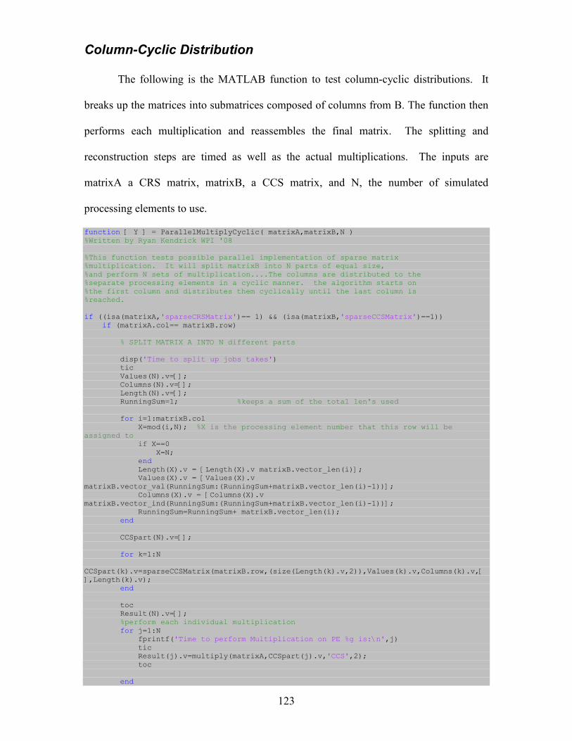
123
Column-Cyclic Distribution
The following is the MATLAB function to test column-cyclic distributions. It
breaks up the matrices into submatrices composed of columns from B. The function then
performs each multiplication and reassembles the final matrix. The splitting and
reconstruction steps are timed as well as the actual multiplications. The inputs are
matrixA a CRS matrix, matrixB, a CCS matrix, and N, the number of simulated
processing elements to use.
function [ Y ] = ParallelMultiplyCyclic( matrixA,matrixB,N ) %Written by Ryan Kendrick WPI '08 %This function tests possible parallel implementation of sparse matrix %multiplication. It will split matrixB into N parts of equal size, %and perform N sets of multiplication....The columns are distributed to the %separate processing elements in a cyclic manner. the algorithm starts on %the first column and distributes them cyclically until the last column is %reached. if ((isa(matrixA,'sparseCRSMatrix')== 1) && (isa(matrixB,'sparseCCSMatrix')==1)) if (matrixA.col== matrixB.row) % SPLIT MATRIX A INTO N different parts disp('Time to split up jobs takes') tic Values(N).v=[]; Columns(N).v=[]; Length(N).v=[]; RunningSum=1; %keeps a sum of the total len's used for i=1:matrixB.col X=mod(i,N); %X is the processing element number that this row will be assigned to if X==0 X=N; end Length(X).v = [Length(X).v matrixB.vector_len(i)]; Values(X).v = [Values(X).v matrixB.vector_val(RunningSum:(RunningSum+matrixB.vector_len(i)-1))]; Columns(X).v = [Columns(X).v matrixB.vector_ind(RunningSum:(RunningSum+matrixB.vector_len(i)-1))]; RunningSum=RunningSum+ matrixB.vector_len(i); end CCSpart(N).v=[]; for k=1:N CCSpart(k).v=sparseCCSMatrix(matrixB.row,(size(Length(k).v,2)),Values(k).v,Columns(k).v,[],Length(k).v); end toc Result(N).v=[]; %perform each individual multiplication for j=1:N fprintf('Time to perform Multiplication on PE %g is:\n',j) tic Result(j).v=multiply(matrixA,CCSpart(j).v,'CCS',2); toc end
124
disp('Final Matrix Construction Takes') tic ValRowLength=0; for d=1:N ValRowLength=ValRowLength+size(Result(d).v.vector_val,2); end FinalValue=zeros(1,ValRowLength); FinalRowIndex=zeros(1,ValRowLength); FinalLength=zeros(1,matrixB.col); Valptr=0; Rowptr=0; LenIndex=1; LenIndexCounter=0; IndexArray=ones(1,N); for h=1:matrixB.col X=mod(h,N); %X is the processing element number that this row will be assigned to if X==0 X=N; end %Assemble Final Length Vector FinalLength(h)= Result(X).v.vector_len(LenIndex); FinalValue((Valptr+1):(Valptr+size(Result(X).v.vector_val(IndexArray(X):(IndexArray(X)+Result(X).v.vector_len(LenIndex)-1)),2))) = Result(X).v.vector_val(IndexArray(X):(IndexArray(X)+Result(X).v.vector_len(LenIndex)-1)); Valptr=Valptr+size(Result(X).v.vector_val(IndexArray(X):(IndexArray(X)+Result(X).v.vector_len(LenIndex)-1)),2); FinalRowIndex((Rowptr+1):(Rowptr+size(Result(X).v.vector_ind(IndexArray(X):(IndexArray(X)+Result(X).v.vector_len(LenIndex)-1)),2))) = Result(X).v.vector_ind(IndexArray(X):(IndexArray(X)+Result(X).v.vector_len(LenIndex)-1)); Rowptr=Rowptr+size(Result(X).v.vector_ind(IndexArray(X):(IndexArray(X)+Result(X).v.vector_len(LenIndex)-1)),2); IndexArray(X)=IndexArray(X)+Result(X).v.vector_len(LenIndex); LenIndexCounter=LenIndexCounter+1; if LenIndexCounter==N LenIndexCounter=0; LenIndex=LenIndex+1; end end Y=sparseCCSMatrix(matrixA.row,matrixB.col,FinalValue,FinalRowIndex,[],FinalLength); toc end end
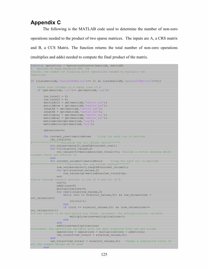
125
Appendix C The following is the MATLAB code used to determine the number of non-zero
operations needed to the product of two sparse matrices. The inputs are A, a CRS matrix
and B, a CCS Matrix. The function returns the total number of non-zero operations
(multiplies and adds) needed to compute the final product of the matrix.
function operations = OperationsCounter(matrixA, matrixB) % Written by Ryan Kendrick WPI '08 %Counts the number of floating point operations needed to multiply two %matrices. if ((isa(matrixA,'sparseCRSMatrix')== 1) && (isa(matrixB,'sparseCCSMatrix')==1)) %make sure columns in A equal rows of B if (get(matrixA,'col')== get(matrixB,'row')) len_total1 = 0; len_total2 = 0; matrixAcol = get(matrixA,'vector_ind'); matrixBrow = get(matrixB,'vector_ind'); lengthA = get(matrixA,'vector_len'); lengthB = get(matrixB,'vector_len'); matrixAval = get(matrixA,'vector_val'); matrixBval = get(matrixB,'vector_val'); matrixArows=get(matrixA,'row'); matrixBcols=get(matrixB,'col'); operations=0; for current_row=1:matrixArows %loop for each row in matrixA len_total2=0; %******************building the col_values vector****** col_values=zeros(1,lengthA(current_row)); for t=1:size(col_values,2) col_values(t)=matrixAcol(len_total1+t); %builds a vector showing which columns there are entries in end for current_column=1:matrixBcols %loop for each col in matrixB %**********************building the row_values vector******** row_values=zeros(1,lengthB(current_column)); for g=1:size(row_values,2) row_values(g)=matrixBrow(len_total2+g); end %Cycle through nonzero entries in row of A and col of B col=1; additions=0; multiplications=0; for row=1:size(row_values,2) while (col <= size(col_values,2)) && row_values(row) > col_values(col) col=col+1; end if ((col <= size(col_values,2)) && (row_values(row)== col_values(col))) %if two values to be multiplied are found, increment the multiplications variable multiplications=multiplications+1; end end additions=multiplications; %increment the operations variable with new data acquired from row and column operations = operations + multiplications + additions; len_total2=len_total2 + size(row_values,2); end len_total1=len_total1 + size(col_values,2); %keeps a cumulative total of all the length values we've used end
126
else error('columns in first matrix must equal rows in the second matrix') end else error('first matrix must be in CRS storage, second must be a CCS') end
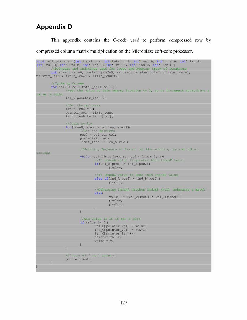
127
Appendix D
This appendix contains the C-code used to perform compressed row by
compressed column matrix multiplication on the Microblaze soft-core processor.
void multiplication(int total_row, int total_col, int* val_A, int* ind_A, int* len_A, int* val_B, int* ind_B, int* len_B, int* val_C, int* ind_C, int* len_C){ //Pointers and indexings used for loops and keeping track of locations int row=0, col=0, pos1=0, pos2=0, value=0, pointer_col=0, pointer_val=0, pointer_len=0, limit_lenA=0, limit_lenB=0; //Cycle by Column for(col=0; col< total_col; col++){ //set the value at this memory location to 0, as to increment everythime a value is added len_C[pointer_len]=0; //Set the pointers limit_lenA = 0; pointer_col = limit_lenB; limit_lenB += len_B[col]; //Cycle by Row for(row=0; row< total_row; row++){ //Set the pointers pos2 = pointer_col; pos1=limit_lenA; limit_lenA += len_A[row]; //Matching Sequence -> Search for the matching row and column indices while(pos1<limit_lenA && pos2 < limit_lenB){ //If indexA value is greater than indexB value if(ind_A[pos1] > ind_B[pos2]) pos2++; //If indexA value is less than indexB value else if(ind_A[pos1] < ind_B[pos2]) pos1++; //Otherwise indexA matches indexB whcih indecates a match else{ value += (val_A[pos1] * val_B[pos2]); pos1++; pos2++; } } //Add value if it is not a zero if(value != 0){ val_C[pointer_val] = value; ind_C[pointer_val] = row+1; len_C[pointer_len]++; pointer_val++; value = 0; } } //Increment length pointer pointer_len++; } }
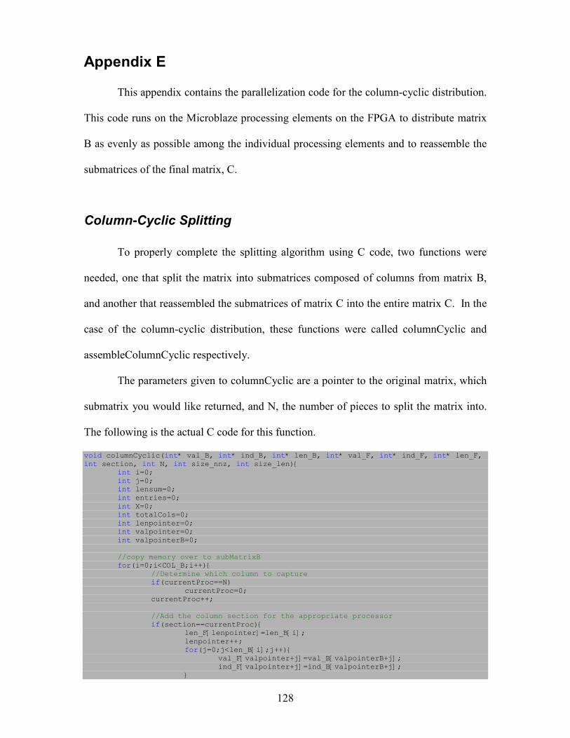
128
Appendix E
This appendix contains the parallelization code for the column-cyclic distribution.
This code runs on the Microblaze processing elements on the FPGA to distribute matrix
B as evenly as possible among the individual processing elements and to reassemble the
submatrices of the final matrix, C.
Column-Cyclic Splitting
To properly complete the splitting algorithm using C code, two functions were
needed, one that split the matrix into submatrices composed of columns from matrix B,
and another that reassembled the submatrices of matrix C into the entire matrix C. In the
case of the column-cyclic distribution, these functions were called columnCyclic and
assembleColumnCyclic respectively.
The parameters given to columnCyclic are a pointer to the original matrix, which
submatrix you would like returned, and N, the number of pieces to split the matrix into.
The following is the actual C code for this function.
void columnCyclic(int* val_B, int* ind_B, int* len_B, int* val_F, int* ind_F, int* len_F, int section, int N, int size_nnz, int size_len){ int i=0; int j=0; int lensum=0; int entries=0; int X=0; int totalCols=0; int lenpointer=0; int valpointer=0; int valpointerB=0; //copy memory over to subMatrixB for(i=0;i<COL_B;i++){ //Determine which column to capture if(currentProc==N) currentProc=0; currentProc++; //Add the column section for the appropriate processor if(section==currentProc){ len_F[lenpointer]=len_B[i]; lenpointer++; for(j=0;j<len_B[i];j++){ val_F[valpointer+j]=val_B[valpointerB+j]; ind_F[valpointer+j]=ind_B[valpointerB+j]; }
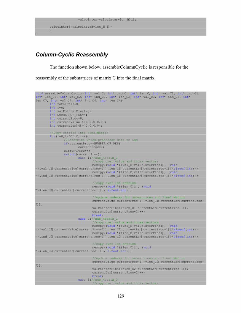
129
valpointer=valpointer+len_B[i]; } valpointerB=valpointerB+len_B[i]; } }
Column-Cyclic Reassembly
The function shown below, assembleColumnCyclic is responsible for the
reassembly of the submatrices of matrix C into the final matrix.
void assembleColumnCyclic(int* val_C, int* ind_C, int* len_C, int* val_C1, int* ind_C1, int* len_C1, int* val_C2, int* ind_C2, int* len_C2, int* val_C3, int* ind_C3, int* len_C3, int* val_C4, int* ind_C4, int* len_C4){ int totalCols=0; int i=0; int valPointerFinal=0; int NUMBER_OF_PES=4; int currentProc=0; int currentValue[4]={0,0,0,0}; int currentLen[4]={0,0,0,0}; //Copy entries into FinalMatrix for(i=0;i<COL_C;i++){ //Determine which processor data to add if(currentProc==NUMBER_OF_PES) currentProc=0; currentProc++; switch(currentProc){ case 1://sub_Matrix_1 //copy over value and index vectors memcpy((void *)&val_C[valPointerFinal], (void *)&val_C1[currentValue[currentProc-1]],len_C1[currentLen[currentProc-1]]*sizeof(int)); memcpy((void *)&ind_C[valPointerFinal], (void *)&ind_C1[currentValue[currentProc-1]],len_C1[currentLen[currentProc-1]]*sizeof(int)); //copy over len entries memcpy((void *)&len_C[i], (void *)&len_C1[currentLen[currentProc-1]], sizeof(int)); //update indexes for submatrices and Final Matrix currentValue[currentProc-1]+=len_C1[currentLen[currentProc-1]]; valPointerFinal+=len_C1[currentLen[currentProc-1]]; currentLen[currentProc-1]++; break; case 2://sub_Matrix_2 //copy over value and index vectors memcpy((void *)&val_C[valPointerFinal], (void *)&val_C2[currentValue[currentProc-1]],len_C2[currentLen[currentProc-1]]*sizeof(int)); memcpy((void *)&ind_C[valPointerFinal], (void *)&ind_C2[currentValue[currentProc-1]],len_C2[currentLen[currentProc-1]]*sizeof(int)); //copy over len entries memcpy((void *)&len_C[i], (void *)&len_C2[currentLen[currentProc-1]], sizeof(int)); //update indexes for submatrices and Final Matrix currentValue[currentProc-1]+=len_C2[currentLen[currentProc-1]]; valPointerFinal+=len_C2[currentLen[currentProc-1]]; currentLen[currentProc-1]++; break; case 3://sub_Matrix_3 //copy over value and index vectors
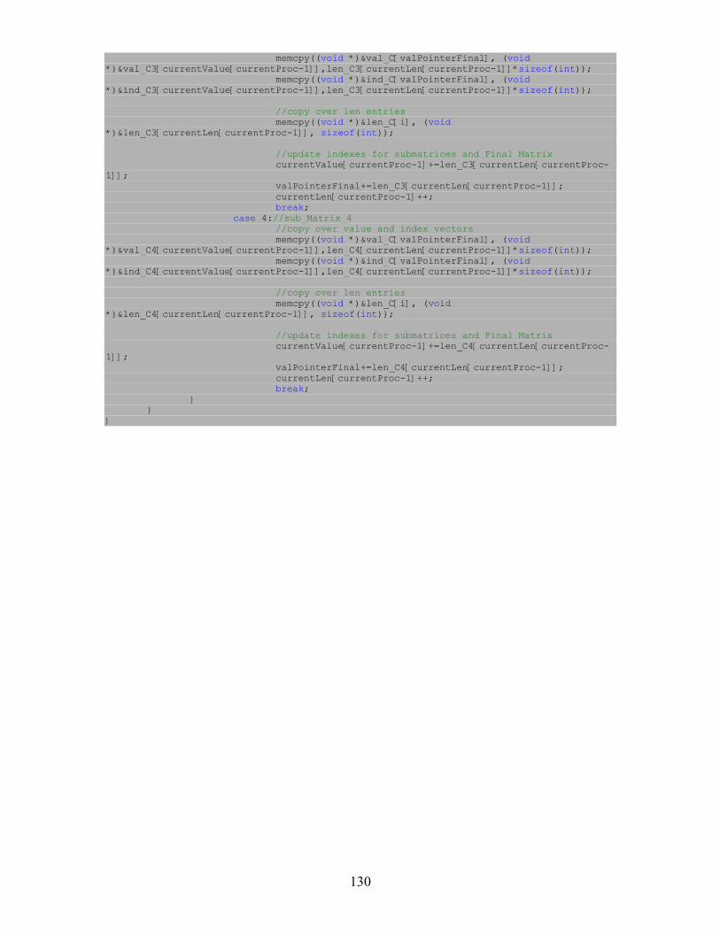
130
memcpy((void *)&val_C[valPointerFinal], (void *)&val_C3[currentValue[currentProc-1]],len_C3[currentLen[currentProc-1]]*sizeof(int)); memcpy((void *)&ind_C[valPointerFinal], (void *)&ind_C3[currentValue[currentProc-1]],len_C3[currentLen[currentProc-1]]*sizeof(int)); //copy over len entries memcpy((void *)&len_C[i], (void *)&len_C3[currentLen[currentProc-1]], sizeof(int)); //update indexes for submatrices and Final Matrix currentValue[currentProc-1]+=len_C3[currentLen[currentProc-1]]; valPointerFinal+=len_C3[currentLen[currentProc-1]]; currentLen[currentProc-1]++; break; case 4://sub_Matrix_4 //copy over value and index vectors memcpy((void *)&val_C[valPointerFinal], (void *)&val_C4[currentValue[currentProc-1]],len_C4[currentLen[currentProc-1]]*sizeof(int)); memcpy((void *)&ind_C[valPointerFinal], (void *)&ind_C4[currentValue[currentProc-1]],len_C4[currentLen[currentProc-1]]*sizeof(int)); //copy over len entries memcpy((void *)&len_C[i], (void *)&len_C4[currentLen[currentProc-1]], sizeof(int)); //update indexes for submatrices and Final Matrix currentValue[currentProc-1]+=len_C4[currentLen[currentProc-1]]; valPointerFinal+=len_C4[currentLen[currentProc-1]]; currentLen[currentProc-1]++; break; } } }
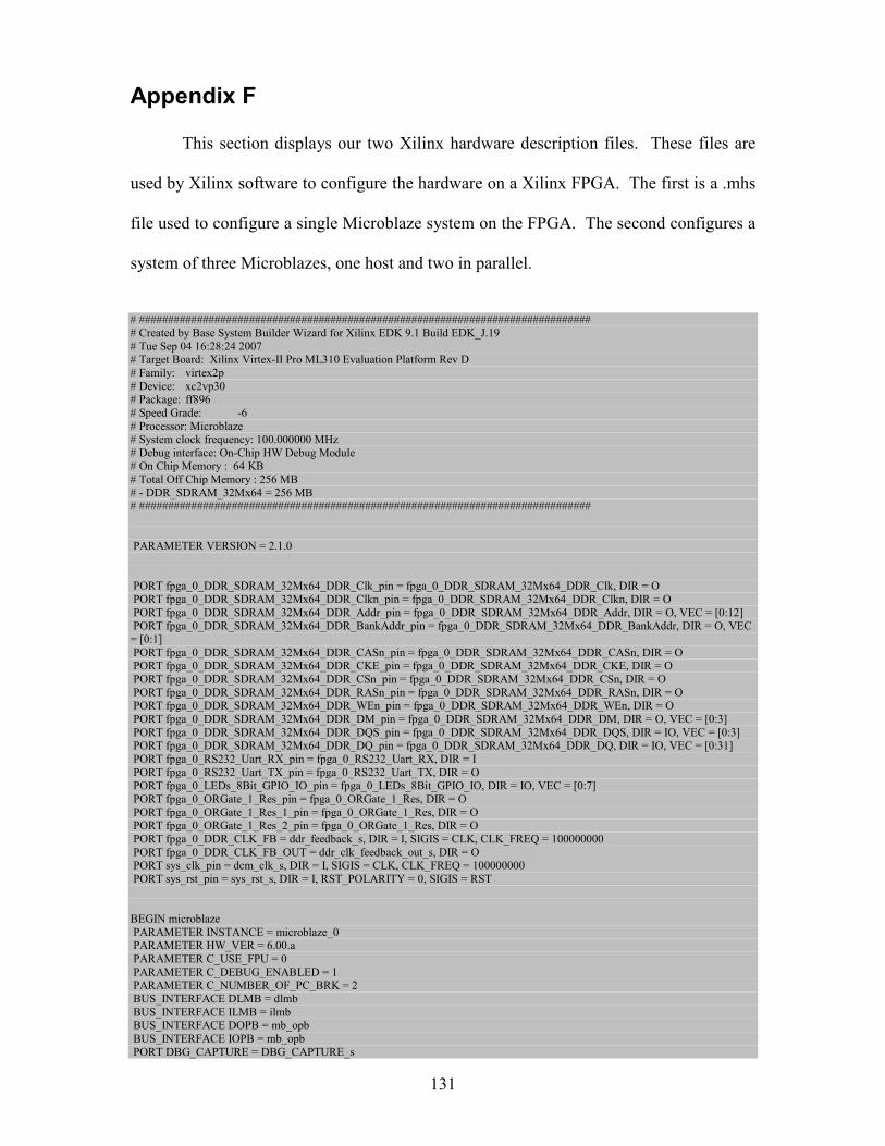
131
Appendix F
This section displays our two Xilinx hardware description files. These files are
used by Xilinx software to configure the hardware on a Xilinx FPGA. The first is a .mhs
file used to configure a single Microblaze system on the FPGA. The second configures a
system of three Microblazes, one host and two in parallel.
# ##############################################################################
# Created by Base System Builder Wizard for Xilinx EDK 9.1 Build EDK_J.19
# Tue Sep 04 16:28:24 2007 # Target Board: Xilinx Virtex-II Pro ML310 Evaluation Platform Rev D
# Family: virtex2p
# Device: xc2vp30 # Package: ff896
# Speed Grade: -6
# Processor: Microblaze # System clock frequency: 100.000000 MHz
# Debug interface: On-Chip HW Debug Module # On Chip Memory : 64 KB
# Total Off Chip Memory : 256 MB
# - DDR_SDRAM_32Mx64 = 256 MB # ##############################################################################
PARAMETER VERSION = 2.1.0
PORT fpga_0_DDR_SDRAM_32Mx64_DDR_Clk_pin = fpga_0_DDR_SDRAM_32Mx64_DDR_Clk, DIR = O
PORT fpga_0_DDR_SDRAM_32Mx64_DDR_Clkn_pin = fpga_0_DDR_SDRAM_32Mx64_DDR_Clkn, DIR = O
PORT fpga_0_DDR_SDRAM_32Mx64_DDR_Addr_pin = fpga_0_DDR_SDRAM_32Mx64_DDR_Addr, DIR = O, VEC = [0:12] PORT fpga_0_DDR_SDRAM_32Mx64_DDR_BankAddr_pin = fpga_0_DDR_SDRAM_32Mx64_DDR_BankAddr, DIR = O, VEC
= [0:1]
PORT fpga_0_DDR_SDRAM_32Mx64_DDR_CASn_pin = fpga_0_DDR_SDRAM_32Mx64_DDR_CASn, DIR = O PORT fpga_0_DDR_SDRAM_32Mx64_DDR_CKE_pin = fpga_0_DDR_SDRAM_32Mx64_DDR_CKE, DIR = O
PORT fpga_0_DDR_SDRAM_32Mx64_DDR_CSn_pin = fpga_0_DDR_SDRAM_32Mx64_DDR_CSn, DIR = O
PORT fpga_0_DDR_SDRAM_32Mx64_DDR_RASn_pin = fpga_0_DDR_SDRAM_32Mx64_DDR_RASn, DIR = O PORT fpga_0_DDR_SDRAM_32Mx64_DDR_WEn_pin = fpga_0_DDR_SDRAM_32Mx64_DDR_WEn, DIR = O
PORT fpga_0_DDR_SDRAM_32Mx64_DDR_DM_pin = fpga_0_DDR_SDRAM_32Mx64_DDR_DM, DIR = O, VEC = [0:3]
PORT fpga_0_DDR_SDRAM_32Mx64_DDR_DQS_pin = fpga_0_DDR_SDRAM_32Mx64_DDR_DQS, DIR = IO, VEC = [0:3] PORT fpga_0_DDR_SDRAM_32Mx64_DDR_DQ_pin = fpga_0_DDR_SDRAM_32Mx64_DDR_DQ, DIR = IO, VEC = [0:31]
PORT fpga_0_RS232_Uart_RX_pin = fpga_0_RS232_Uart_RX, DIR = I
PORT fpga_0_RS232_Uart_TX_pin = fpga_0_RS232_Uart_TX, DIR = O PORT fpga_0_LEDs_8Bit_GPIO_IO_pin = fpga_0_LEDs_8Bit_GPIO_IO, DIR = IO, VEC = [0:7]
PORT fpga_0_ORGate_1_Res_pin = fpga_0_ORGate_1_Res, DIR = O
PORT fpga_0_ORGate_1_Res_1_pin = fpga_0_ORGate_1_Res, DIR = O PORT fpga_0_ORGate_1_Res_2_pin = fpga_0_ORGate_1_Res, DIR = O
PORT fpga_0_DDR_CLK_FB = ddr_feedback_s, DIR = I, SIGIS = CLK, CLK_FREQ = 100000000
PORT fpga_0_DDR_CLK_FB_OUT = ddr_clk_feedback_out_s, DIR = O PORT sys_clk_pin = dcm_clk_s, DIR = I, SIGIS = CLK, CLK_FREQ = 100000000
PORT sys_rst_pin = sys_rst_s, DIR = I, RST_POLARITY = 0, SIGIS = RST
BEGIN microblaze
PARAMETER INSTANCE = microblaze_0 PARAMETER HW_VER = 6.00.a
PARAMETER C_USE_FPU = 0
PARAMETER C_DEBUG_ENABLED = 1 PARAMETER C_NUMBER_OF_PC_BRK = 2
BUS_INTERFACE DLMB = dlmb
BUS_INTERFACE ILMB = ilmb BUS_INTERFACE DOPB = mb_opb
BUS_INTERFACE IOPB = mb_opb
PORT DBG_CAPTURE = DBG_CAPTURE_s
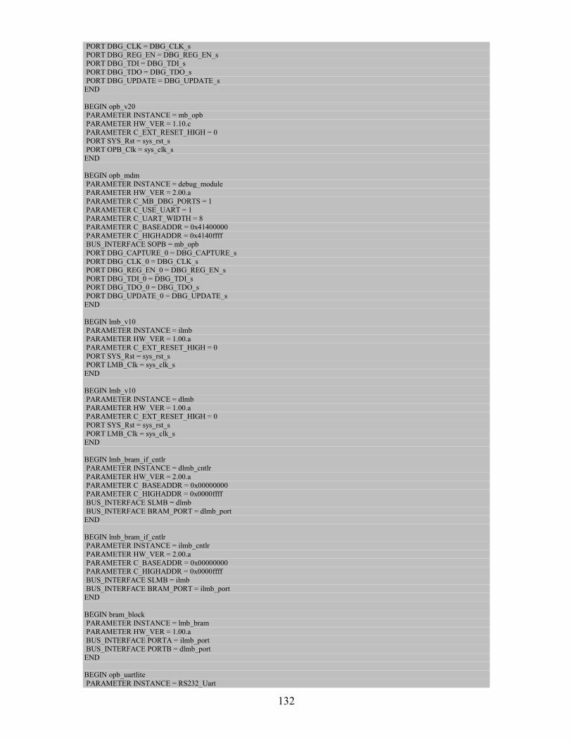
132
PORT DBG_CLK = DBG_CLK_s
PORT DBG_REG_EN = DBG_REG_EN_s PORT DBG_TDI = DBG_TDI_s
PORT DBG_TDO = DBG_TDO_s
PORT DBG_UPDATE = DBG_UPDATE_s END
BEGIN opb_v20 PARAMETER INSTANCE = mb_opb
PARAMETER HW_VER = 1.10.c
PARAMETER C_EXT_RESET_HIGH = 0 PORT SYS_Rst = sys_rst_s
PORT OPB_Clk = sys_clk_s
END
BEGIN opb_mdm
PARAMETER INSTANCE = debug_module PARAMETER HW_VER = 2.00.a
PARAMETER C_MB_DBG_PORTS = 1
PARAMETER C_USE_UART = 1 PARAMETER C_UART_WIDTH = 8
PARAMETER C_BASEADDR = 0x41400000
PARAMETER C_HIGHADDR = 0x4140ffff BUS_INTERFACE SOPB = mb_opb
PORT DBG_CAPTURE_0 = DBG_CAPTURE_s
PORT DBG_CLK_0 = DBG_CLK_s PORT DBG_REG_EN_0 = DBG_REG_EN_s
PORT DBG_TDI_0 = DBG_TDI_s PORT DBG_TDO_0 = DBG_TDO_s
PORT DBG_UPDATE_0 = DBG_UPDATE_s
END
BEGIN lmb_v10
PARAMETER INSTANCE = ilmb PARAMETER HW_VER = 1.00.a
PARAMETER C_EXT_RESET_HIGH = 0
PORT SYS_Rst = sys_rst_s PORT LMB_Clk = sys_clk_s
END
BEGIN lmb_v10
PARAMETER INSTANCE = dlmb
PARAMETER HW_VER = 1.00.a PARAMETER C_EXT_RESET_HIGH = 0
PORT SYS_Rst = sys_rst_s
PORT LMB_Clk = sys_clk_s END
BEGIN lmb_bram_if_cntlr PARAMETER INSTANCE = dlmb_cntlr
PARAMETER HW_VER = 2.00.a
PARAMETER C_BASEADDR = 0x00000000 PARAMETER C_HIGHADDR = 0x0000ffff
BUS_INTERFACE SLMB = dlmb
BUS_INTERFACE BRAM_PORT = dlmb_port END
BEGIN lmb_bram_if_cntlr PARAMETER INSTANCE = ilmb_cntlr
PARAMETER HW_VER = 2.00.a
PARAMETER C_BASEADDR = 0x00000000 PARAMETER C_HIGHADDR = 0x0000ffff
BUS_INTERFACE SLMB = ilmb
BUS_INTERFACE BRAM_PORT = ilmb_port END
BEGIN bram_block PARAMETER INSTANCE = lmb_bram
PARAMETER HW_VER = 1.00.a
BUS_INTERFACE PORTA = ilmb_port BUS_INTERFACE PORTB = dlmb_port
END
BEGIN opb_uartlite
PARAMETER INSTANCE = RS232_Uart
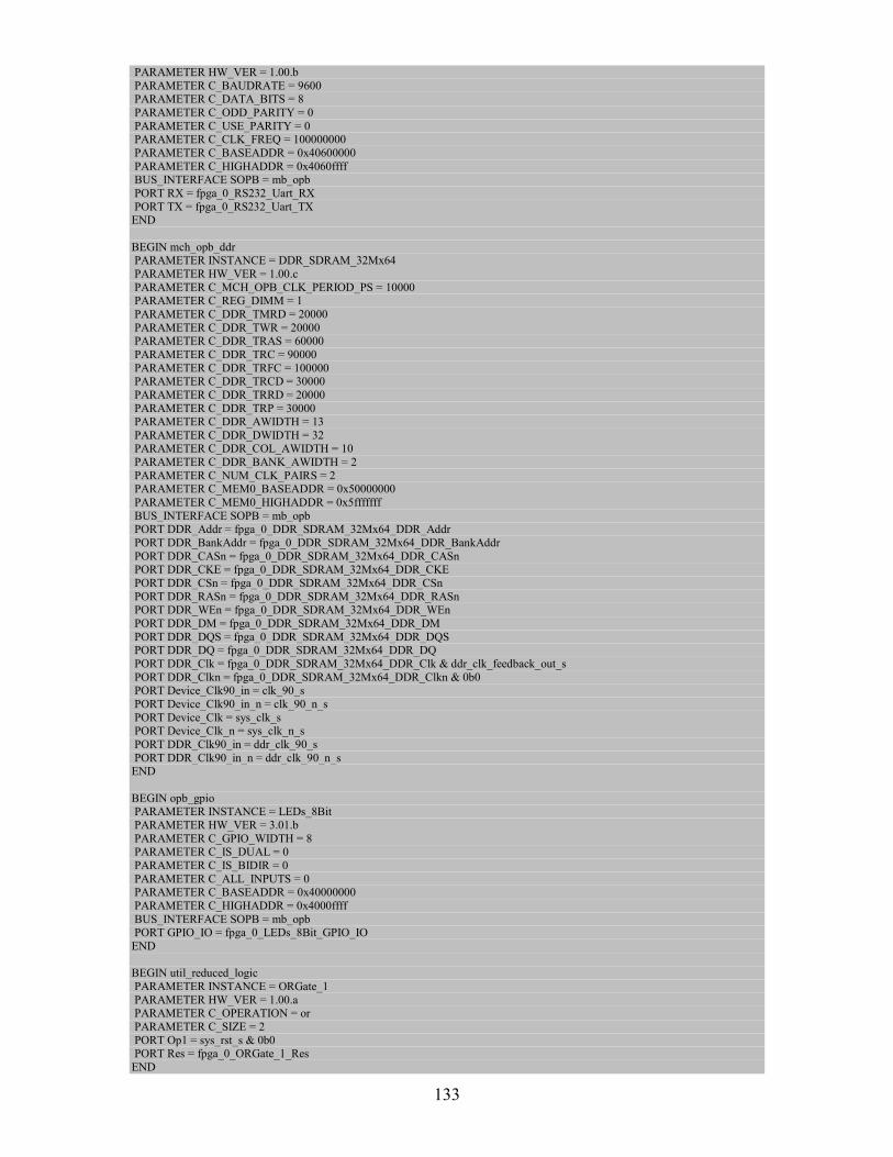
133
PARAMETER HW_VER = 1.00.b
PARAMETER C_BAUDRATE = 9600 PARAMETER C_DATA_BITS = 8
PARAMETER C_ODD_PARITY = 0
PARAMETER C_USE_PARITY = 0 PARAMETER C_CLK_FREQ = 100000000
PARAMETER C_BASEADDR = 0x40600000
PARAMETER C_HIGHADDR = 0x4060ffff BUS_INTERFACE SOPB = mb_opb
PORT RX = fpga_0_RS232_Uart_RX
PORT TX = fpga_0_RS232_Uart_TX END
BEGIN mch_opb_ddr PARAMETER INSTANCE = DDR_SDRAM_32Mx64
PARAMETER HW_VER = 1.00.c
PARAMETER C_MCH_OPB_CLK_PERIOD_PS = 10000 PARAMETER C_REG_DIMM = 1
PARAMETER C_DDR_TMRD = 20000
PARAMETER C_DDR_TWR = 20000 PARAMETER C_DDR_TRAS = 60000
PARAMETER C_DDR_TRC = 90000
PARAMETER C_DDR_TRFC = 100000 PARAMETER C_DDR_TRCD = 30000
PARAMETER C_DDR_TRRD = 20000
PARAMETER C_DDR_TRP = 30000 PARAMETER C_DDR_AWIDTH = 13
PARAMETER C_DDR_DWIDTH = 32 PARAMETER C_DDR_COL_AWIDTH = 10
PARAMETER C_DDR_BANK_AWIDTH = 2
PARAMETER C_NUM_CLK_PAIRS = 2 PARAMETER C_MEM0_BASEADDR = 0x50000000
PARAMETER C_MEM0_HIGHADDR = 0x5fffffff
BUS_INTERFACE SOPB = mb_opb PORT DDR_Addr = fpga_0_DDR_SDRAM_32Mx64_DDR_Addr
PORT DDR_BankAddr = fpga_0_DDR_SDRAM_32Mx64_DDR_BankAddr
PORT DDR_CASn = fpga_0_DDR_SDRAM_32Mx64_DDR_CASn PORT DDR_CKE = fpga_0_DDR_SDRAM_32Mx64_DDR_CKE
PORT DDR_CSn = fpga_0_DDR_SDRAM_32Mx64_DDR_CSn
PORT DDR_RASn = fpga_0_DDR_SDRAM_32Mx64_DDR_RASn PORT DDR_WEn = fpga_0_DDR_SDRAM_32Mx64_DDR_WEn
PORT DDR_DM = fpga_0_DDR_SDRAM_32Mx64_DDR_DM
PORT DDR_DQS = fpga_0_DDR_SDRAM_32Mx64_DDR_DQS PORT DDR_DQ = fpga_0_DDR_SDRAM_32Mx64_DDR_DQ
PORT DDR_Clk = fpga_0_DDR_SDRAM_32Mx64_DDR_Clk & ddr_clk_feedback_out_s
PORT DDR_Clkn = fpga_0_DDR_SDRAM_32Mx64_DDR_Clkn & 0b0 PORT Device_Clk90_in = clk_90_s
PORT Device_Clk90_in_n = clk_90_n_s
PORT Device_Clk = sys_clk_s PORT Device_Clk_n = sys_clk_n_s
PORT DDR_Clk90_in = ddr_clk_90_s
PORT DDR_Clk90_in_n = ddr_clk_90_n_s END
BEGIN opb_gpio PARAMETER INSTANCE = LEDs_8Bit
PARAMETER HW_VER = 3.01.b
PARAMETER C_GPIO_WIDTH = 8 PARAMETER C_IS_DUAL = 0
PARAMETER C_IS_BIDIR = 0
PARAMETER C_ALL_INPUTS = 0 PARAMETER C_BASEADDR = 0x40000000
PARAMETER C_HIGHADDR = 0x4000ffff
BUS_INTERFACE SOPB = mb_opb PORT GPIO_IO = fpga_0_LEDs_8Bit_GPIO_IO
END
BEGIN util_reduced_logic
PARAMETER INSTANCE = ORGate_1
PARAMETER HW_VER = 1.00.a PARAMETER C_OPERATION = or
PARAMETER C_SIZE = 2
PORT Op1 = sys_rst_s & 0b0 PORT Res = fpga_0_ORGate_1_Res
END
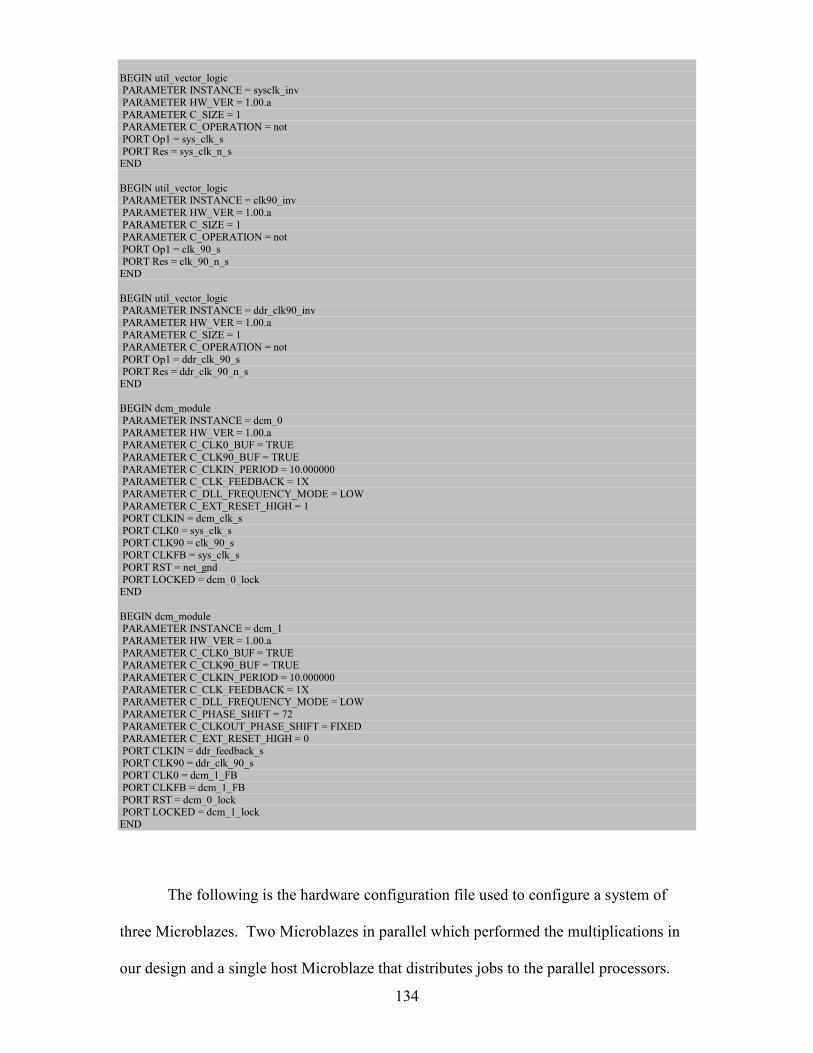
134
BEGIN util_vector_logic PARAMETER INSTANCE = sysclk_inv
PARAMETER HW_VER = 1.00.a
PARAMETER C_SIZE = 1 PARAMETER C_OPERATION = not
PORT Op1 = sys_clk_s
PORT Res = sys_clk_n_s END
BEGIN util_vector_logic PARAMETER INSTANCE = clk90_inv
PARAMETER HW_VER = 1.00.a
PARAMETER C_SIZE = 1 PARAMETER C_OPERATION = not
PORT Op1 = clk_90_s
PORT Res = clk_90_n_s END
BEGIN util_vector_logic PARAMETER INSTANCE = ddr_clk90_inv
PARAMETER HW_VER = 1.00.a
PARAMETER C_SIZE = 1 PARAMETER C_OPERATION = not
PORT Op1 = ddr_clk_90_s
PORT Res = ddr_clk_90_n_s END
BEGIN dcm_module
PARAMETER INSTANCE = dcm_0
PARAMETER HW_VER = 1.00.a PARAMETER C_CLK0_BUF = TRUE
PARAMETER C_CLK90_BUF = TRUE
PARAMETER C_CLKIN_PERIOD = 10.000000 PARAMETER C_CLK_FEEDBACK = 1X
PARAMETER C_DLL_FREQUENCY_MODE = LOW
PARAMETER C_EXT_RESET_HIGH = 1 PORT CLKIN = dcm_clk_s
PORT CLK0 = sys_clk_s
PORT CLK90 = clk_90_s PORT CLKFB = sys_clk_s
PORT RST = net_gnd
PORT LOCKED = dcm_0_lock END
BEGIN dcm_module PARAMETER INSTANCE = dcm_1
PARAMETER HW_VER = 1.00.a
PARAMETER C_CLK0_BUF = TRUE PARAMETER C_CLK90_BUF = TRUE
PARAMETER C_CLKIN_PERIOD = 10.000000
PARAMETER C_CLK_FEEDBACK = 1X PARAMETER C_DLL_FREQUENCY_MODE = LOW
PARAMETER C_PHASE_SHIFT = 72
PARAMETER C_CLKOUT_PHASE_SHIFT = FIXED PARAMETER C_EXT_RESET_HIGH = 0
PORT CLKIN = ddr_feedback_s
PORT CLK90 = ddr_clk_90_s PORT CLK0 = dcm_1_FB
PORT CLKFB = dcm_1_FB
PORT RST = dcm_0_lock PORT LOCKED = dcm_1_lock
END
The following is the hardware configuration file used to configure a system of
three Microblazes. Two Microblazes in parallel which performed the multiplications in
our design and a single host Microblaze that distributes jobs to the parallel processors.
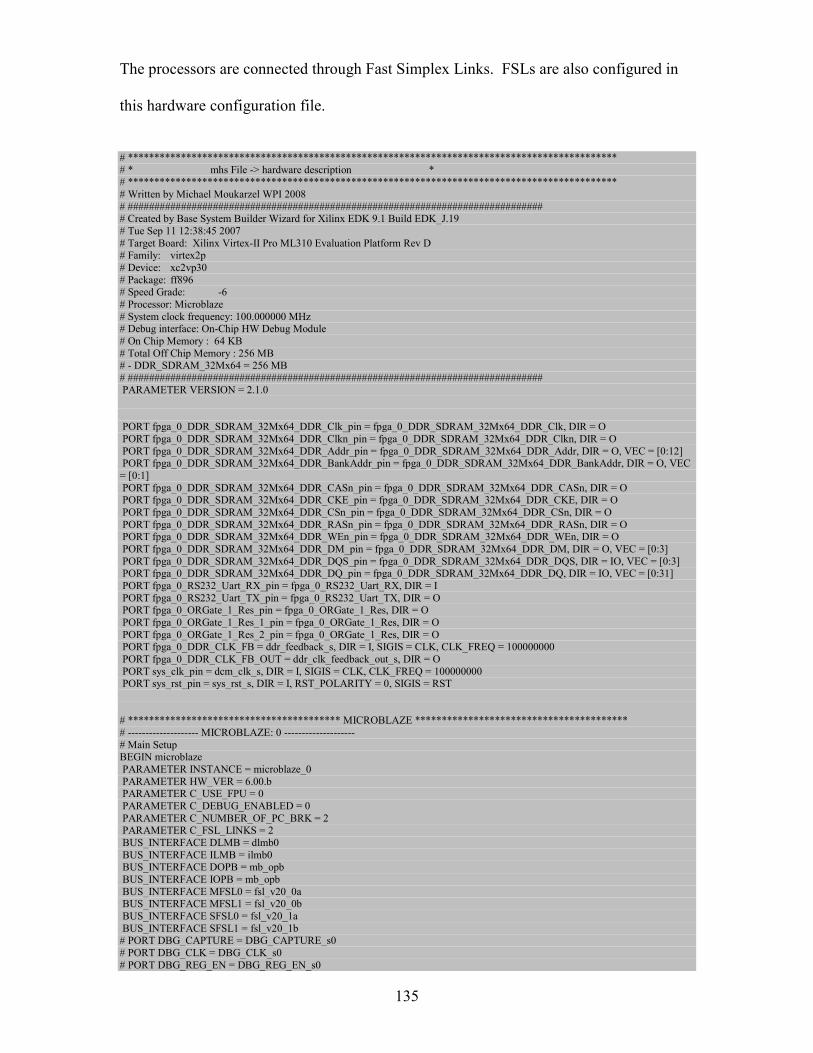
135
The processors are connected through Fast Simplex Links. FSLs are also configured in
this hardware configuration file.
# ********************************************************************************************
# * mhs File -> hardware description * # ********************************************************************************************
# Written by Michael Moukarzel WPI 2008
# ############################################################################## # Created by Base System Builder Wizard for Xilinx EDK 9.1 Build EDK_J.19
# Tue Sep 11 12:38:45 2007
# Target Board: Xilinx Virtex-II Pro ML310 Evaluation Platform Rev D # Family: virtex2p
# Device: xc2vp30
# Package: ff896 # Speed Grade: -6
# Processor: Microblaze
# System clock frequency: 100.000000 MHz # Debug interface: On-Chip HW Debug Module
# On Chip Memory : 64 KB
# Total Off Chip Memory : 256 MB # - DDR_SDRAM_32Mx64 = 256 MB
# ############################################################################## PARAMETER VERSION = 2.1.0
PORT fpga_0_DDR_SDRAM_32Mx64_DDR_Clk_pin = fpga_0_DDR_SDRAM_32Mx64_DDR_Clk, DIR = O
PORT fpga_0_DDR_SDRAM_32Mx64_DDR_Clkn_pin = fpga_0_DDR_SDRAM_32Mx64_DDR_Clkn, DIR = O
PORT fpga_0_DDR_SDRAM_32Mx64_DDR_Addr_pin = fpga_0_DDR_SDRAM_32Mx64_DDR_Addr, DIR = O, VEC = [0:12] PORT fpga_0_DDR_SDRAM_32Mx64_DDR_BankAddr_pin = fpga_0_DDR_SDRAM_32Mx64_DDR_BankAddr, DIR = O, VEC
= [0:1]
PORT fpga_0_DDR_SDRAM_32Mx64_DDR_CASn_pin = fpga_0_DDR_SDRAM_32Mx64_DDR_CASn, DIR = O PORT fpga_0_DDR_SDRAM_32Mx64_DDR_CKE_pin = fpga_0_DDR_SDRAM_32Mx64_DDR_CKE, DIR = O
PORT fpga_0_DDR_SDRAM_32Mx64_DDR_CSn_pin = fpga_0_DDR_SDRAM_32Mx64_DDR_CSn, DIR = O
PORT fpga_0_DDR_SDRAM_32Mx64_DDR_RASn_pin = fpga_0_DDR_SDRAM_32Mx64_DDR_RASn, DIR = O PORT fpga_0_DDR_SDRAM_32Mx64_DDR_WEn_pin = fpga_0_DDR_SDRAM_32Mx64_DDR_WEn, DIR = O
PORT fpga_0_DDR_SDRAM_32Mx64_DDR_DM_pin = fpga_0_DDR_SDRAM_32Mx64_DDR_DM, DIR = O, VEC = [0:3]
PORT fpga_0_DDR_SDRAM_32Mx64_DDR_DQS_pin = fpga_0_DDR_SDRAM_32Mx64_DDR_DQS, DIR = IO, VEC = [0:3] PORT fpga_0_DDR_SDRAM_32Mx64_DDR_DQ_pin = fpga_0_DDR_SDRAM_32Mx64_DDR_DQ, DIR = IO, VEC = [0:31]
PORT fpga_0_RS232_Uart_RX_pin = fpga_0_RS232_Uart_RX, DIR = I
PORT fpga_0_RS232_Uart_TX_pin = fpga_0_RS232_Uart_TX, DIR = O PORT fpga_0_ORGate_1_Res_pin = fpga_0_ORGate_1_Res, DIR = O
PORT fpga_0_ORGate_1_Res_1_pin = fpga_0_ORGate_1_Res, DIR = O
PORT fpga_0_ORGate_1_Res_2_pin = fpga_0_ORGate_1_Res, DIR = O PORT fpga_0_DDR_CLK_FB = ddr_feedback_s, DIR = I, SIGIS = CLK, CLK_FREQ = 100000000
PORT fpga_0_DDR_CLK_FB_OUT = ddr_clk_feedback_out_s, DIR = O
PORT sys_clk_pin = dcm_clk_s, DIR = I, SIGIS = CLK, CLK_FREQ = 100000000 PORT sys_rst_pin = sys_rst_s, DIR = I, RST_POLARITY = 0, SIGIS = RST
# **************************************** MICROBLAZE ****************************************
# -------------------- MICROBLAZE: 0 --------------------
# Main Setup BEGIN microblaze
PARAMETER INSTANCE = microblaze_0
PARAMETER HW_VER = 6.00.b PARAMETER C_USE_FPU = 0
PARAMETER C_DEBUG_ENABLED = 0
PARAMETER C_NUMBER_OF_PC_BRK = 2 PARAMETER C_FSL_LINKS = 2
BUS_INTERFACE DLMB = dlmb0
BUS_INTERFACE ILMB = ilmb0 BUS_INTERFACE DOPB = mb_opb
BUS_INTERFACE IOPB = mb_opb
BUS_INTERFACE MFSL0 = fsl_v20_0a BUS_INTERFACE MFSL1 = fsl_v20_0b
BUS_INTERFACE SFSL0 = fsl_v20_1a
BUS_INTERFACE SFSL1 = fsl_v20_1b # PORT DBG_CAPTURE = DBG_CAPTURE_s0
# PORT DBG_CLK = DBG_CLK_s0
# PORT DBG_REG_EN = DBG_REG_EN_s0
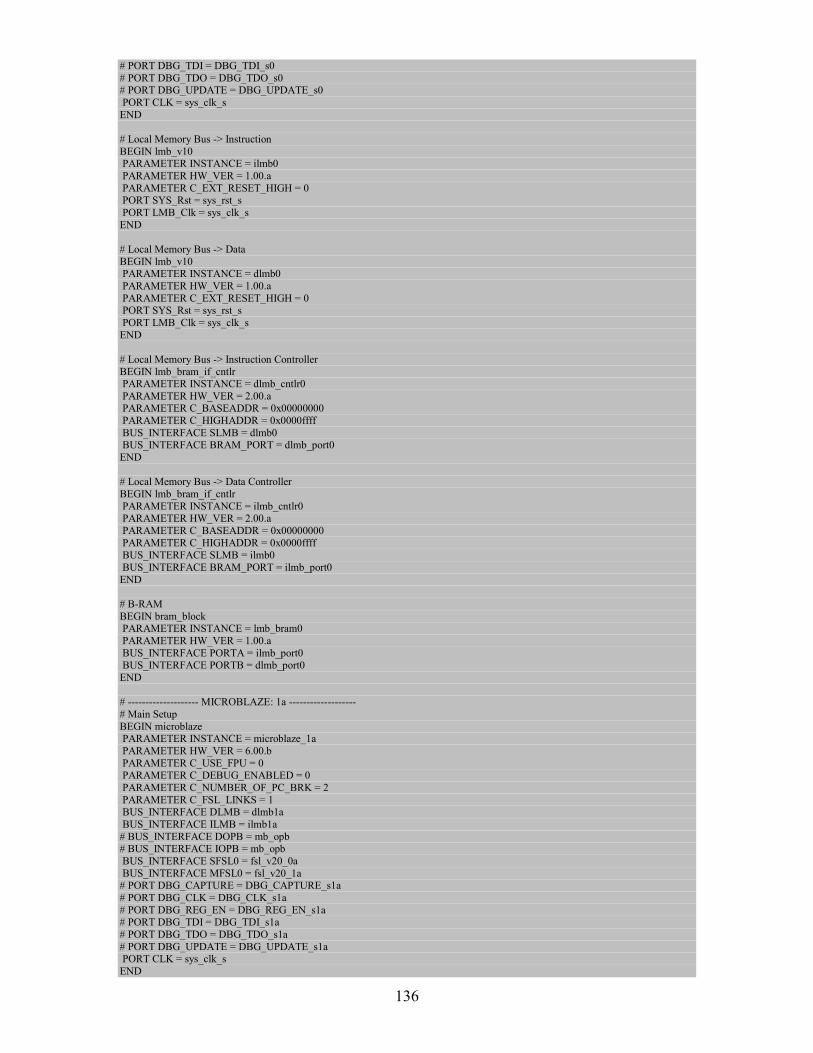
136
# PORT DBG_TDI = DBG_TDI_s0
# PORT DBG_TDO = DBG_TDO_s0 # PORT DBG_UPDATE = DBG_UPDATE_s0
PORT CLK = sys_clk_s
END
# Local Memory Bus -> Instruction
BEGIN lmb_v10 PARAMETER INSTANCE = ilmb0
PARAMETER HW_VER = 1.00.a
PARAMETER C_EXT_RESET_HIGH = 0 PORT SYS_Rst = sys_rst_s
PORT LMB_Clk = sys_clk_s
END
# Local Memory Bus -> Data
BEGIN lmb_v10 PARAMETER INSTANCE = dlmb0
PARAMETER HW_VER = 1.00.a
PARAMETER C_EXT_RESET_HIGH = 0 PORT SYS_Rst = sys_rst_s
PORT LMB_Clk = sys_clk_s
END
# Local Memory Bus -> Instruction Controller
BEGIN lmb_bram_if_cntlr PARAMETER INSTANCE = dlmb_cntlr0
PARAMETER HW_VER = 2.00.a PARAMETER C_BASEADDR = 0x00000000
PARAMETER C_HIGHADDR = 0x0000ffff
BUS_INTERFACE SLMB = dlmb0 BUS_INTERFACE BRAM_PORT = dlmb_port0
END
# Local Memory Bus -> Data Controller
BEGIN lmb_bram_if_cntlr
PARAMETER INSTANCE = ilmb_cntlr0 PARAMETER HW_VER = 2.00.a
PARAMETER C_BASEADDR = 0x00000000
PARAMETER C_HIGHADDR = 0x0000ffff BUS_INTERFACE SLMB = ilmb0
BUS_INTERFACE BRAM_PORT = ilmb_port0
END
# B-RAM
BEGIN bram_block PARAMETER INSTANCE = lmb_bram0
PARAMETER HW_VER = 1.00.a
BUS_INTERFACE PORTA = ilmb_port0 BUS_INTERFACE PORTB = dlmb_port0
END
# -------------------- MICROBLAZE: 1a -------------------
# Main Setup
BEGIN microblaze PARAMETER INSTANCE = microblaze_1a
PARAMETER HW_VER = 6.00.b
PARAMETER C_USE_FPU = 0 PARAMETER C_DEBUG_ENABLED = 0
PARAMETER C_NUMBER_OF_PC_BRK = 2
PARAMETER C_FSL_LINKS = 1 BUS_INTERFACE DLMB = dlmb1a
BUS_INTERFACE ILMB = ilmb1a
# BUS_INTERFACE DOPB = mb_opb # BUS_INTERFACE IOPB = mb_opb
BUS_INTERFACE SFSL0 = fsl_v20_0a
BUS_INTERFACE MFSL0 = fsl_v20_1a # PORT DBG_CAPTURE = DBG_CAPTURE_s1a
# PORT DBG_CLK = DBG_CLK_s1a
# PORT DBG_REG_EN = DBG_REG_EN_s1a # PORT DBG_TDI = DBG_TDI_s1a
# PORT DBG_TDO = DBG_TDO_s1a
# PORT DBG_UPDATE = DBG_UPDATE_s1a PORT CLK = sys_clk_s
END
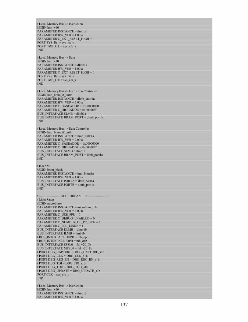
137
# Local Memory Bus -> Instruction BEGIN lmb_v10
PARAMETER INSTANCE = ilmb1a
PARAMETER HW_VER = 1.00.a PARAMETER C_EXT_RESET_HIGH = 0
PORT SYS_Rst = sys_rst_s
PORT LMB_Clk = sys_clk_s END
# Local Memory Bus -> Data BEGIN lmb_v10
PARAMETER INSTANCE = dlmb1a
PARAMETER HW_VER = 1.00.a PARAMETER C_EXT_RESET_HIGH = 0
PORT SYS_Rst = sys_rst_s
PORT LMB_Clk = sys_clk_s END
# Local Memory Bus -> Instruction Controller BEGIN lmb_bram_if_cntlr
PARAMETER INSTANCE = dlmb_cntlr1a
PARAMETER HW_VER = 2.00.a PARAMETER C_BASEADDR = 0x00000000
PARAMETER C_HIGHADDR = 0x0000ffff
BUS_INTERFACE SLMB = dlmb1a BUS_INTERFACE BRAM_PORT = dlmb_port1a
END
# Local Memory Bus -> Data Controller
BEGIN lmb_bram_if_cntlr PARAMETER INSTANCE = ilmb_cntlr1a
PARAMETER HW_VER = 2.00.a
PARAMETER C_BASEADDR = 0x00000000 PARAMETER C_HIGHADDR = 0x0000ffff
BUS_INTERFACE SLMB = ilmb1a
BUS_INTERFACE BRAM_PORT = ilmb_port1a END
# B-RAM BEGIN bram_block
PARAMETER INSTANCE = lmb_bram1a
PARAMETER HW_VER = 1.00.a BUS_INTERFACE PORTA = ilmb_port1a
BUS_INTERFACE PORTB = dlmb_port1a
END
# -------------------- MICROBLAZE: 1b -------------------
# Main Setup BEGIN microblaze
PARAMETER INSTANCE = microblaze_1b
PARAMETER HW_VER = 6.00.b PARAMETER C_USE_FPU = 0
PARAMETER C_DEBUG_ENABLED = 0
PARAMETER C_NUMBER_OF_PC_BRK = 2 PARAMETER C_FSL_LINKS = 1
BUS_INTERFACE DLMB = dlmb1b
BUS_INTERFACE ILMB = ilmb1b # BUS_INTERFACE DOPB = mb_opb
# BUS_INTERFACE IOPB = mb_opb
BUS_INTERFACE SFSL0 = fsl_v20_0b BUS_INTERFACE MFSL0 = fsl_v20_1b
# PORT DBG_CAPTURE = DBG_CAPTURE_s1b
# PORT DBG_CLK = DBG_CLK_s1b # PORT DBG_REG_EN = DBG_REG_EN_s1b
# PORT DBG_TDI = DBG_TDI_s1b
# PORT DBG_TDO = DBG_TDO_s1b # PORT DBG_UPDATE = DBG_UPDATE_s1b
PORT CLK = sys_clk_s
END
# Local Memory Bus -> Instruction
BEGIN lmb_v10 PARAMETER INSTANCE = ilmb1b
PARAMETER HW_VER = 1.00.a
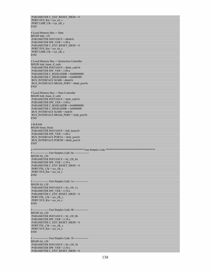
138
PARAMETER C_EXT_RESET_HIGH = 0
PORT SYS_Rst = sys_rst_s PORT LMB_Clk = sys_clk_s
END
# Local Memory Bus -> Data
BEGIN lmb_v10
PARAMETER INSTANCE = dlmb1b PARAMETER HW_VER = 1.00.a
PARAMETER C_EXT_RESET_HIGH = 0
PORT SYS_Rst = sys_rst_s PORT LMB_Clk = sys_clk_s
END
# Local Memory Bus -> Instruction Controller
BEGIN lmb_bram_if_cntlr
PARAMETER INSTANCE = dlmb_cntlr1b PARAMETER HW_VER = 2.00.a
PARAMETER C_BASEADDR = 0x00000000
PARAMETER C_HIGHADDR = 0x0000ffff BUS_INTERFACE SLMB = dlmb1b
BUS_INTERFACE BRAM_PORT = dlmb_port1b
END
# Local Memory Bus -> Data Controller
BEGIN lmb_bram_if_cntlr PARAMETER INSTANCE = ilmb_cntlr1b
PARAMETER HW_VER = 2.00.a PARAMETER C_BASEADDR = 0x00000000
PARAMETER C_HIGHADDR = 0x0000ffff
BUS_INTERFACE SLMB = ilmb1b BUS_INTERFACE BRAM_PORT = ilmb_port1b
END
# B-RAM
BEGIN bram_block
PARAMETER INSTANCE = lmb_bram1b PARAMETER HW_VER = 1.00.a
BUS_INTERFACE PORTA = ilmb_port1b
BUS_INTERFACE PORTB = dlmb_port1b END
# ************************************* Fast Simplex Link ************************************ # ----------------- Fast Simplex Link: 0a ----------------
BEGIN fsl_v20
PARAMETER INSTANCE = fsl_v20_0a PARAMETER HW_VER = 2.10.a
PARAMETER C_EXT_RESET_HIGH = 0
PORT FSL_Clk = sys_clk_s PORT SYS_Rst = sys_rst_s
END
# ----------------- Fast Simplex Link: 1a ---------------
BEGIN fsl_v20
PARAMETER INSTANCE = fsl_v20_1a PARAMETER HW_VER = 2.10.a
PARAMETER C_EXT_RESET_HIGH = 0
PORT FSL_Clk = sys_clk_s PORT SYS_Rst = sys_rst_s
END
# ----------------- Fast Simplex Link: 0b ---------------
BEGIN fsl_v20
PARAMETER INSTANCE = fsl_v20_0b PARAMETER HW_VER = 2.10.a
PARAMETER C_EXT_RESET_HIGH = 0
PORT FSL_Clk = sys_clk_s PORT SYS_Rst = sys_rst_s
END
# ----------------- Fast Simplex Link: 1b ---------------
BEGIN fsl_v20
PARAMETER INSTANCE = fsl_v20_1b PARAMETER HW_VER = 2.10.a
PARAMETER C_EXT_RESET_HIGH = 0
139
PORT FSL_Clk = sys_clk_s
PORT SYS_Rst = sys_rst_s END
# ********************************** On Chip Perifferal Bus ********************************** BEGIN opb_v20
PARAMETER INSTANCE = mb_opb
PARAMETER HW_VER = 1.10.c PARAMETER C_EXT_RESET_HIGH = 0
PORT SYS_Rst = sys_rst_s
PORT OPB_Clk = sys_clk_s END
# ************************* Slaves of On Chip Perifferal Bus(mb_opb) ************************* # ---------------------- DDR Memory ---------------------
BEGIN mch_opb_ddr
PARAMETER INSTANCE = DDR_SDRAM_32Mx64 PARAMETER HW_VER = 1.00.c
PARAMETER C_MCH_OPB_CLK_PERIOD_PS = 10000
PARAMETER C_REG_DIMM = 1 PARAMETER C_DDR_TMRD = 20000
PARAMETER C_DDR_TWR = 20000
PARAMETER C_DDR_TRAS = 60000 PARAMETER C_DDR_TRC = 90000
PARAMETER C_DDR_TRFC = 100000
PARAMETER C_DDR_TRCD = 30000 PARAMETER C_DDR_TRRD = 20000
PARAMETER C_DDR_TRP = 30000 PARAMETER C_DDR_AWIDTH = 13
PARAMETER C_DDR_DWIDTH = 32
PARAMETER C_DDR_COL_AWIDTH = 10 PARAMETER C_DDR_BANK_AWIDTH = 2
PARAMETER C_NUM_CLK_PAIRS = 2
PARAMETER C_MEM0_BASEADDR = 0x50000000 PARAMETER C_MEM0_HIGHADDR = 0x5fffffff
BUS_INTERFACE SOPB = mb_opb
PORT DDR_Addr = fpga_0_DDR_SDRAM_32Mx64_DDR_Addr PORT DDR_BankAddr = fpga_0_DDR_SDRAM_32Mx64_DDR_BankAddr
PORT DDR_CASn = fpga_0_DDR_SDRAM_32Mx64_DDR_CASn
PORT DDR_CKE = fpga_0_DDR_SDRAM_32Mx64_DDR_CKE PORT DDR_CSn = fpga_0_DDR_SDRAM_32Mx64_DDR_CSn
PORT DDR_RASn = fpga_0_DDR_SDRAM_32Mx64_DDR_RASn
PORT DDR_WEn = fpga_0_DDR_SDRAM_32Mx64_DDR_WEn PORT DDR_DM = fpga_0_DDR_SDRAM_32Mx64_DDR_DM
PORT DDR_DQS = fpga_0_DDR_SDRAM_32Mx64_DDR_DQS
PORT DDR_DQ = fpga_0_DDR_SDRAM_32Mx64_DDR_DQ PORT DDR_Clk = fpga_0_DDR_SDRAM_32Mx64_DDR_Clk & ddr_clk_feedback_out_s
PORT DDR_Clkn = fpga_0_DDR_SDRAM_32Mx64_DDR_Clkn & 0b0
PORT Device_Clk90_in = clk_90_s PORT Device_Clk90_in_n = clk_90_n_s
PORT Device_Clk = sys_clk_s
PORT Device_Clk_n = sys_clk_n_s PORT DDR_Clk90_in = ddr_clk_90_s
PORT DDR_Clk90_in_n = ddr_clk_90_n_s
END
# ------------------- Serial Interface ------------------
BEGIN opb_uartlite PARAMETER INSTANCE = RS232_Uart
PARAMETER HW_VER = 1.00.b
PARAMETER C_BAUDRATE = 9600 PARAMETER C_DATA_BITS = 8
PARAMETER C_ODD_PARITY = 0
PARAMETER C_USE_PARITY = 0 PARAMETER C_CLK_FREQ = 100000000
PARAMETER C_BASEADDR = 0x40600000
PARAMETER C_HIGHADDR = 0x4060ffff BUS_INTERFACE SOPB = mb_opb
PORT RX = fpga_0_RS232_Uart_RX
PORT TX = fpga_0_RS232_Uart_TX END
# ----------------------- Debugger ---------------------- # BEGIN opb_mdm
# PARAMETER INSTANCE = debug_module
140
# PARAMETER HW_VER = 2.00.a
# PARAMETER C_MB_DBG_PORTS = 1 # PARAMETER C_USE_UART = 1
# PARAMETER C_UART_WIDTH = 8
# PARAMETER C_BASEADDR = 0x41400000 # PARAMETER C_HIGHADDR = 0x4140ffff
# BUS_INTERFACE SOPB = mb_opb
# PORT DBG_CAPTURE_0 = DBG_CAPTURE_s0 # PORT DBG_CLK_0 = DBG_CLK_s0
# PORT DBG_REG_EN_0 = DBG_REG_EN_s0
# PORT DBG_TDI_0 = DBG_TDI_s0 # PORT DBG_TDO_0 = DBG_TDO_s0
# PORT DBG_UPDATE_0 = DBG_UPDATE_s0
# PORT DBG_CAPTURE_1 = DBG_CAPTURE_s1a # PORT DBG_CLK_1 = DBG_CLK_s1a
# PORT DBG_REG_EN_1 = DBG_REG_EN_s1a
# PORT DBG_TDI_1 = DBG_TDI_s1a # PORT DBG_TDO_1 = DBG_TDO_s1a
# PORT DBG_UPDATE_1 = DBG_UPDATE_s1a
# PORT DBG_CAPTURE_3 = DBG_CAPTURE_s1b # PORT DBG_CLK_3 = DBG_CLK_s1b
# PORT DBG_REG_EN_3 = DBG_REG_EN_s1b
# PORT DBG_TDI_3 = DBG_TDI_s1b # PORT DBG_TDO_3 = DBG_TDO_s1b
# PORT DBG_UPDATE_3 = DBG_UPDATE_s1b
# END # ******************************** IP - Intellectual Property ********************************
# ----------------------- Or Gate ----------------------- BEGIN util_reduced_logic
PARAMETER INSTANCE = ORGate_1
PARAMETER HW_VER = 1.00.a PARAMETER C_OPERATION = or
PARAMETER C_SIZE = 2
PORT Op1 = sys_rst_s & 0b0 PORT Res = fpga_0_ORGate_1_Res
END
# --------------- System Clock (inverted) ---------------
BEGIN util_vector_logic
PARAMETER INSTANCE = sysclk_inv PARAMETER HW_VER = 1.00.a
PARAMETER C_SIZE = 1
PARAMETER C_OPERATION = not PORT Op1 = sys_clk_s
PORT Res = sys_clk_n_s
END
# --------- Clock (inverted and 90 phase shift) ---------
BEGIN util_vector_logic PARAMETER INSTANCE = clk90_inv
PARAMETER HW_VER = 1.00.a
PARAMETER C_SIZE = 1 PARAMETER C_OPERATION = not
PORT Op1 = clk_90_s
PORT Res = clk_90_n_s END
# ------- DDR Clock (inverted and 90 phase shift) ------- BEGIN util_vector_logic
PARAMETER INSTANCE = ddr_clk90_inv
PARAMETER HW_VER = 1.00.a PARAMETER C_SIZE = 1
PARAMETER C_OPERATION = not
PORT Op1 = ddr_clk_90_s PORT Res = ddr_clk_90_n_s
END
# ----------- Digital Clock Managers -> dcm_0 -----------
BEGIN dcm_module
PARAMETER INSTANCE = dcm_0 PARAMETER HW_VER = 1.00.c
PARAMETER C_CLK0_BUF = TRUE
PARAMETER C_CLK90_BUF = TRUE PARAMETER C_CLKIN_PERIOD = 10.000000
PARAMETER C_CLK_FEEDBACK = 1X
141
PARAMETER C_DLL_FREQUENCY_MODE = LOW
PARAMETER C_EXT_RESET_HIGH = 1 PORT CLKIN = dcm_clk_s
PORT CLK0 = sys_clk_s
PORT CLK90 = clk_90_s PORT CLKFB = sys_clk_s
PORT RST = net_gnd
PORT LOCKED = dcm_0_lock END
# ----------- Digital Clock Managers -> dcm_1 ----------- BEGIN dcm_module
PARAMETER INSTANCE = dcm_1
PARAMETER HW_VER = 1.00.c PARAMETER C_CLK0_BUF = TRUE
PARAMETER C_CLK90_BUF = TRUE
PARAMETER C_CLKIN_PERIOD = 10.000000 PARAMETER C_CLK_FEEDBACK = 1X
PARAMETER C_DLL_FREQUENCY_MODE = LOW
PARAMETER C_PHASE_SHIFT = 72 PARAMETER C_CLKOUT_PHASE_SHIFT = FIXED
PARAMETER C_EXT_RESET_HIGH = 0
PORT CLKIN = ddr_feedback_s PORT CLK90 = ddr_clk_90_s
PORT CLK0 = dcm_1_FB
PORT CLKFB = dcm_1_FB PORT RST = dcm_0_lock
PORT LOCKED = dcm_1_lock END
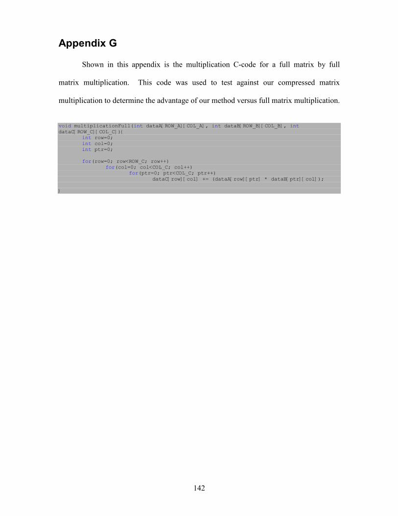
142
Appendix G
Shown in this appendix is the multiplication C-code for a full matrix by full
matrix multiplication. This code was used to test against our compressed matrix
multiplication to determine the advantage of our method versus full matrix multiplication.
void multiplicationFull(int dataA[ROW_A][COL_A], int dataB[ROW_B][COL_B], int dataC[ROW_C][COL_C]){ int row=0; int col=0; int ptr=0; for(row=0; row<ROW_C; row++) for(col=0; col<COL_C; col++) for(ptr=0; ptr<COL_C; ptr++) dataC[row][col] += (dataA[row][ptr] * dataB[ptr][col]); }
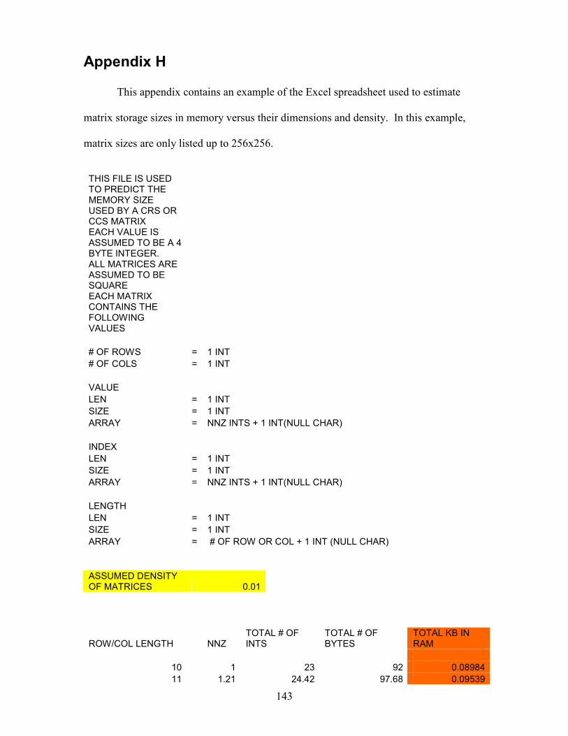
143
Appendix H
This appendix contains an example of the Excel spreadsheet used to estimate
matrix storage sizes in memory versus their dimensions and density. In this example,
matrix sizes are only listed up to 256x256.
THIS FILE IS USED TO PREDICT THE MEMORY SIZE USED BY A CRS OR CCS MATRIX EACH VALUE IS ASSUMED TO BE A 4 BYTE INTEGER. ALL MATRICES ARE ASSUMED TO BE SQUARE EACH MATRIX CONTAINS THE FOLLOWING VALUES
# OF ROWS = 1 INT
# OF COLS = 1 INT
VALUE
LEN = 1 INT
SIZE = 1 INT
ARRAY = NNZ INTS + 1 INT(NULL CHAR)
INDEX
LEN = 1 INT
SIZE = 1 INT
ARRAY = NNZ INTS + 1 INT(NULL CHAR)
LENGTH
LEN = 1 INT
SIZE = 1 INT
ARRAY = # OF ROW OR COL + 1 INT (NULL CHAR)
ASSUMED DENSITY OF MATRICES 0.01
ROW/COL LENGTH NNZ TOTAL # OF INTS
TOTAL # OF BYTES
TOTAL KB IN RAM
10 1 23 92 0.08984
11 1.21 24.42 97.68 0.09539
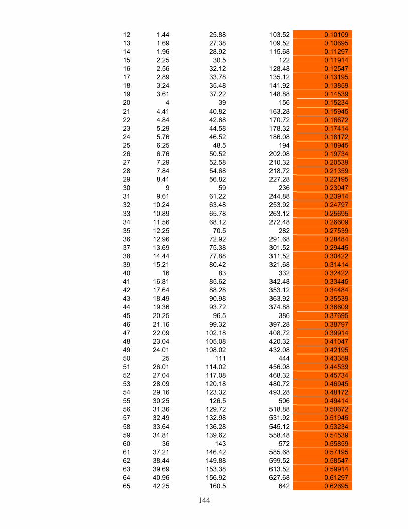
144
12 1.44 25.88 103.52 0.10109
13 1.69 27.38 109.52 0.10695
14 1.96 28.92 115.68 0.11297
15 2.25 30.5 122 0.11914
16 2.56 32.12 128.48 0.12547
17 2.89 33.78 135.12 0.13195
18 3.24 35.48 141.92 0.13859
19 3.61 37.22 148.88 0.14539
20 4 39 156 0.15234
21 4.41 40.82 163.28 0.15945
22 4.84 42.68 170.72 0.16672
23 5.29 44.58 178.32 0.17414
24 5.76 46.52 186.08 0.18172
25 6.25 48.5 194 0.18945
26 6.76 50.52 202.08 0.19734
27 7.29 52.58 210.32 0.20539
28 7.84 54.68 218.72 0.21359
29 8.41 56.82 227.28 0.22195
30 9 59 236 0.23047
31 9.61 61.22 244.88 0.23914
32 10.24 63.48 253.92 0.24797
33 10.89 65.78 263.12 0.25695
34 11.56 68.12 272.48 0.26609
35 12.25 70.5 282 0.27539
36 12.96 72.92 291.68 0.28484
37 13.69 75.38 301.52 0.29445
38 14.44 77.88 311.52 0.30422
39 15.21 80.42 321.68 0.31414
40 16 83 332 0.32422
41 16.81 85.62 342.48 0.33445
42 17.64 88.28 353.12 0.34484
43 18.49 90.98 363.92 0.35539
44 19.36 93.72 374.88 0.36609
45 20.25 96.5 386 0.37695
46 21.16 99.32 397.28 0.38797
47 22.09 102.18 408.72 0.39914
48 23.04 105.08 420.32 0.41047
49 24.01 108.02 432.08 0.42195
50 25 111 444 0.43359
51 26.01 114.02 456.08 0.44539
52 27.04 117.08 468.32 0.45734
53 28.09 120.18 480.72 0.46945
54 29.16 123.32 493.28 0.48172
55 30.25 126.5 506 0.49414
56 31.36 129.72 518.88 0.50672
57 32.49 132.98 531.92 0.51945
58 33.64 136.28 545.12 0.53234
59 34.81 139.62 558.48 0.54539
60 36 143 572 0.55859
61 37.21 146.42 585.68 0.57195
62 38.44 149.88 599.52 0.58547
63 39.69 153.38 613.52 0.59914
64 40.96 156.92 627.68 0.61297
65 42.25 160.5 642 0.62695
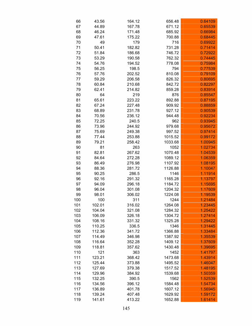
145
66 43.56 164.12 656.48 0.64109
67 44.89 167.78 671.12 0.65539
68 46.24 171.48 685.92 0.66984
69 47.61 175.22 700.88 0.68445
70 49 179 716 0.69922
71 50.41 182.82 731.28 0.71414
72 51.84 186.68 746.72 0.72922
73 53.29 190.58 762.32 0.74445
74 54.76 194.52 778.08 0.75984
75 56.25 198.5 794 0.77539
76 57.76 202.52 810.08 0.79109
77 59.29 206.58 826.32 0.80695
78 60.84 210.68 842.72 0.82297
79 62.41 214.82 859.28 0.83914
80 64 219 876 0.85547
81 65.61 223.22 892.88 0.87195
82 67.24 227.48 909.92 0.88859
83 68.89 231.78 927.12 0.90539
84 70.56 236.12 944.48 0.92234
85 72.25 240.5 962 0.93945
86 73.96 244.92 979.68 0.95672
87 75.69 249.38 997.52 0.97414
88 77.44 253.88 1015.52 0.99172
89 79.21 258.42 1033.68 1.00945
90 81 263 1052 1.02734
91 82.81 267.62 1070.48 1.04539
92 84.64 272.28 1089.12 1.06359
93 86.49 276.98 1107.92 1.08195
94 88.36 281.72 1126.88 1.10047
95 90.25 286.5 1146 1.11914
96 92.16 291.32 1165.28 1.13797
97 94.09 296.18 1184.72 1.15695
98 96.04 301.08 1204.32 1.17609
99 98.01 306.02 1224.08 1.19539
100 100 311 1244 1.21484
101 102.01 316.02 1264.08 1.23445
102 104.04 321.08 1284.32 1.25422
103 106.09 326.18 1304.72 1.27414
104 108.16 331.32 1325.28 1.29422
105 110.25 336.5 1346 1.31445
106 112.36 341.72 1366.88 1.33484
107 114.49 346.98 1387.92 1.35539
108 116.64 352.28 1409.12 1.37609
109 118.81 357.62 1430.48 1.39695
110 121 363 1452 1.41797
111 123.21 368.42 1473.68 1.43914
112 125.44 373.88 1495.52 1.46047
113 127.69 379.38 1517.52 1.48195
114 129.96 384.92 1539.68 1.50359
115 132.25 390.5 1562 1.52539
116 134.56 396.12 1584.48 1.54734
117 136.89 401.78 1607.12 1.56945
118 139.24 407.48 1629.92 1.59172
119 141.61 413.22 1652.88 1.61414
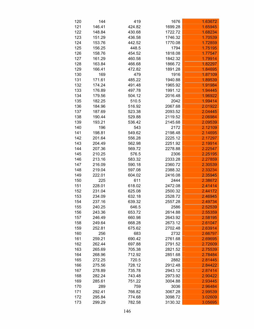
146
120 144 419 1676 1.63672
121 146.41 424.82 1699.28 1.65945
122 148.84 430.68 1722.72 1.68234
123 151.29 436.58 1746.32 1.70539
124 153.76 442.52 1770.08 1.72859
125 156.25 448.5 1794 1.75195
126 158.76 454.52 1818.08 1.77547
127 161.29 460.58 1842.32 1.79914
128 163.84 466.68 1866.72 1.82297
129 166.41 472.82 1891.28 1.84695
130 169 479 1916 1.87109
131 171.61 485.22 1940.88 1.89539
132 174.24 491.48 1965.92 1.91984
133 176.89 497.78 1991.12 1.94445
134 179.56 504.12 2016.48 1.96922
135 182.25 510.5 2042 1.99414
136 184.96 516.92 2067.68 2.01922
137 187.69 523.38 2093.52 2.04445
138 190.44 529.88 2119.52 2.06984
139 193.21 536.42 2145.68 2.09539
140 196 543 2172 2.12109
141 198.81 549.62 2198.48 2.14695
142 201.64 556.28 2225.12 2.17297
143 204.49 562.98 2251.92 2.19914
144 207.36 569.72 2278.88 2.22547
145 210.25 576.5 2306 2.25195
146 213.16 583.32 2333.28 2.27859
147 216.09 590.18 2360.72 2.30539
148 219.04 597.08 2388.32 2.33234
149 222.01 604.02 2416.08 2.35945
150 225 611 2444 2.38672
151 228.01 618.02 2472.08 2.41414
152 231.04 625.08 2500.32 2.44172
153 234.09 632.18 2528.72 2.46945
154 237.16 639.32 2557.28 2.49734
155 240.25 646.5 2586 2.52539
156 243.36 653.72 2614.88 2.55359
157 246.49 660.98 2643.92 2.58195
158 249.64 668.28 2673.12 2.61047
159 252.81 675.62 2702.48 2.63914
160 256 683 2732 2.66797
161 259.21 690.42 2761.68 2.69695
162 262.44 697.88 2791.52 2.72609
163 265.69 705.38 2821.52 2.75539
164 268.96 712.92 2851.68 2.78484
165 272.25 720.5 2882 2.81445
166 275.56 728.12 2912.48 2.84422
167 278.89 735.78 2943.12 2.87414
168 282.24 743.48 2973.92 2.90422
169 285.61 751.22 3004.88 2.93445
170 289 759 3036 2.96484
171 292.41 766.82 3067.28 2.99539
172 295.84 774.68 3098.72 3.02609
173 299.29 782.58 3130.32 3.05695
147
174 302.76 790.52 3162.08 3.08797
175 306.25 798.5 3194 3.11914
176 309.76 806.52 3226.08 3.15047
177 313.29 814.58 3258.32 3.18195
178 316.84 822.68 3290.72 3.21359
179 320.41 830.82 3323.28 3.24539
180 324 839 3356 3.27734
181 327.61 847.22 3388.88 3.30945
182 331.24 855.48 3421.92 3.34172
183 334.89 863.78 3455.12 3.37414
184 338.56 872.12 3488.48 3.40672
185 342.25 880.5 3522 3.43945
186 345.96 888.92 3555.68 3.47234
187 349.69 897.38 3589.52 3.50539
188 353.44 905.88 3623.52 3.53859
189 357.21 914.42 3657.68 3.57195
190 361 923 3692 3.60547
191 364.81 931.62 3726.48 3.63914
192 368.64 940.28 3761.12 3.67297
193 372.49 948.98 3795.92 3.70695
194 376.36 957.72 3830.88 3.74109
195 380.25 966.5 3866 3.77539
196 384.16 975.32 3901.28 3.80984
197 388.09 984.18 3936.72 3.84445
198 392.04 993.08 3972.32 3.87922
199 396.01 1002.02 4008.08 3.91414
200 400 1011 4044 3.94922
201 404.01 1020.02 4080.08 3.98445
202 408.04 1029.08 4116.32 4.01984
203 412.09 1038.18 4152.72 4.05539
204 416.16 1047.32 4189.28 4.09109
205 420.25 1056.5 4226 4.12695
206 424.36 1065.72 4262.88 4.16297
207 428.49 1074.98 4299.92 4.19914
208 432.64 1084.28 4337.12 4.23547
209 436.81 1093.62 4374.48 4.27195
210 441 1103 4412 4.30859
211 445.21 1112.42 4449.68 4.34539
212 449.44 1121.88 4487.52 4.38234
213 453.69 1131.38 4525.52 4.41945
214 457.96 1140.92 4563.68 4.45672
215 462.25 1150.5 4602 4.49414
216 466.56 1160.12 4640.48 4.53172
217 470.89 1169.78 4679.12 4.56945
218 475.24 1179.48 4717.92 4.60734
219 479.61 1189.22 4756.88 4.64539
220 484 1199 4796 4.68359
221 488.41 1208.82 4835.28 4.72195
222 492.84 1218.68 4874.72 4.76047
223 497.29 1228.58 4914.32 4.79914
224 501.76 1238.52 4954.08 4.83797
225 506.25 1248.5 4994 4.87695
226 510.76 1258.52 5034.08 4.91609
227 515.29 1268.58 5074.32 4.95539
148
228 519.84 1278.68 5114.72 4.99484
229 524.41 1288.82 5155.28 5.03445
230 529 1299 5196 5.07422
231 533.61 1309.22 5236.88 5.11414
232 538.24 1319.48 5277.92 5.15422
233 542.89 1329.78 5319.12 5.19445
234 547.56 1340.12 5360.48 5.23484
235 552.25 1350.5 5402 5.27539
236 556.96 1360.92 5443.68 5.31609
237 561.69 1371.38 5485.52 5.35695
238 566.44 1381.88 5527.52 5.39797
239 571.21 1392.42 5569.68 5.43914
240 576 1403 5612 5.48047
241 580.81 1413.62 5654.48 5.52195
242 585.64 1424.28 5697.12 5.56359
243 590.49 1434.98 5739.92 5.60539
244 595.36 1445.72 5782.88 5.64734
245 600.25 1456.5 5826 5.68945
246 605.16 1467.32 5869.28 5.73172
247 610.09 1478.18 5912.72 5.77414
248 615.04 1489.08 5956.32 5.81672
249 620.01 1500.02 6000.08 5.85945
250 625 1511 6044 5.90234
251 630.01 1522.02 6088.08 5.94539
252 635.04 1533.08 6132.32 5.98859
253 640.09 1544.18 6176.72 6.03195
254 645.16 1555.32 6221.28 6.07547
255 650.25 1566.5 6266 6.11914
256 655.36 1577.72 6310.88 6.16297
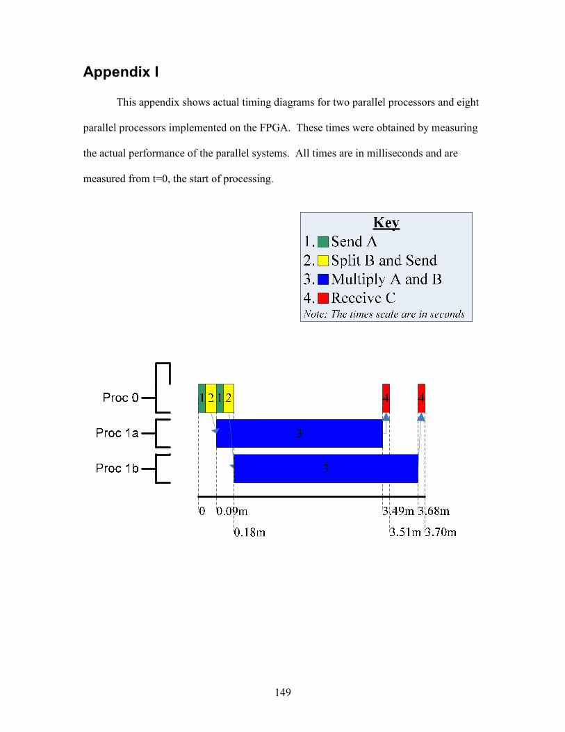
149
Appendix I
This appendix shows actual timing diagrams for two parallel processors and eight
parallel processors implemented on the FPGA. These times were obtained by measuring
the actual performance of the parallel systems. All times are in milliseconds and are
measured from t=0, the start of processing.
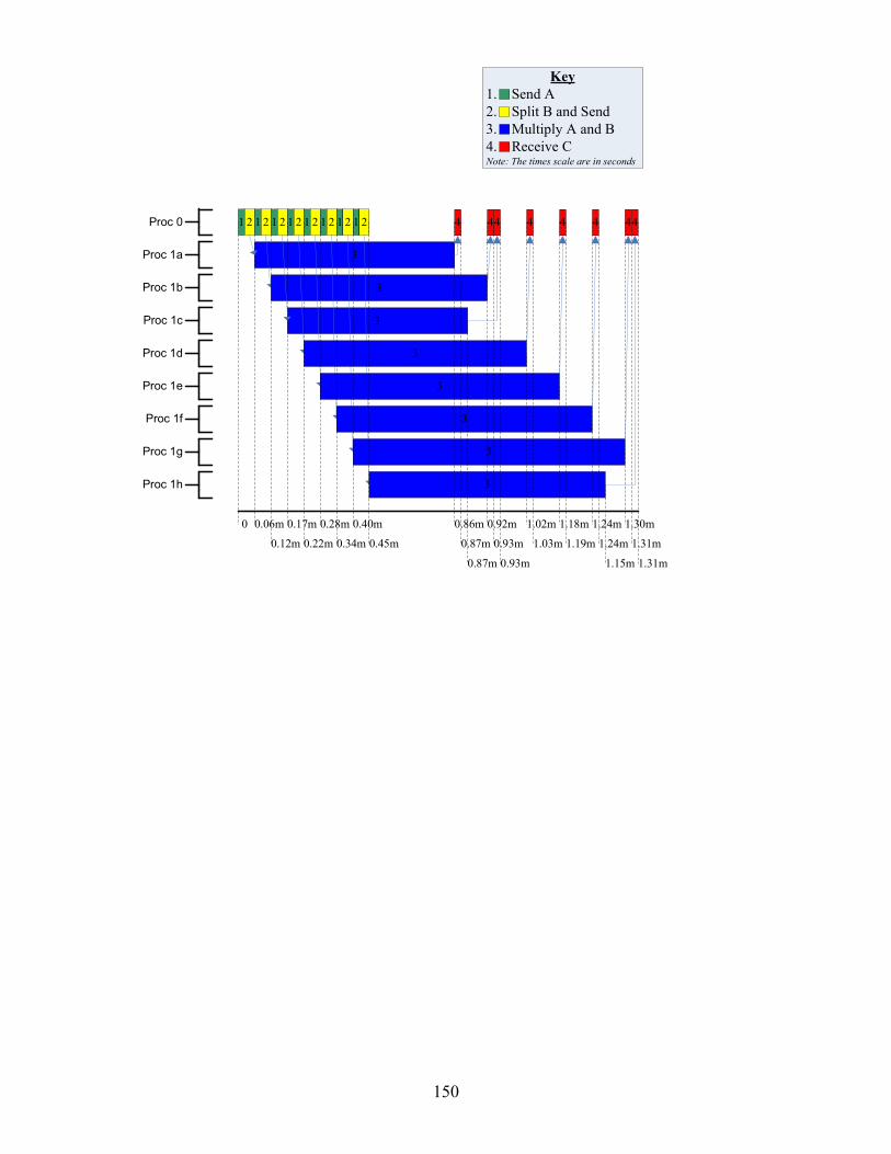
150
3
3
1 2 41 2 4Proc 0
Proc 1a
Proc 1b 3
1 2 1 2 1 2 1 2 1 2 1 2
3
3
3
3
3
0 0.06m
0.12m
0.17m
0.22m
0.28m
0.34m
4
0.87m
1.02m 1.18m 1.24m 1.30m
1.15m
0.40m
0.45m 0.93m
0.86m 0.92m
1.03m 1.19m 1.24m 1.31m
1.31m
4444 4
0.87m
Proc 1c
Proc 1d
Proc 1e
Proc 1f
Proc 1g
Proc 1h
Key
1. Send A
2. Split B and Send
3. Multiply A and B
4. Receive CNote: The times scale are in seconds
0.93m
151
Appendix J
This appendix contains a complete flow chart for the implementation of a logic
circuit to perform the matrix by matrix multiplication algorithm in logic rather than in C-
code on a microprocessor. Implementation of parallel logic circuits of this type could be
used to significantly increase the performance of the compressed-row times compressed
column multiplication kernel.
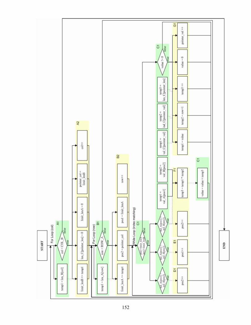
152

153
IEEE Code of Ethics
We, the members of the IEEE, in recognition of the importance of our technologies in
affecting the qualify of life throughout the world, and in accepting a personal obligation
to our profession, its members, and the communities we serve, do hereby commit
ourselves to the highest ethical and professional conduct and agree:
1. To accept responsibility in making decisions consistent with the safety, health and
welfare of the public, and to disclose promptly factors that might endanger the
public of the environment;
2. to avoid real or perceived conflicts of interest whenever possible, and to disclose
them to affected parties when they do exist;
3. to be honest and realistic in stating claims or estimates based on available data;
4. to reject bribery in all its forms;
5. to improve on the understanding of technology, its appropriate application, and
potential consequences;
6. to maintain and improve our technical competencies and to undertake
technological tasks for others only if qualified by training or experience, or after
full disclosure of pertinent limitations;
7. to seek, accept and offer honest criticism of technical work, to acknowledge and
correct errors, and to credit properly the contributions of others;
8. to treat fairly all persons regardless of such factors as race, religion, gender,
disability, age, or national origin;
9. to avoid injuring others, their property, reputation, or employment by false or
malicious action;
10. to assist colleagues and co-workers in their professional development and to
support them in following this code of ethics.
The IEEE code of ethics applies in multiple ways to this Major Qualifying Project
experience. A few examples of how this applied to this experience follow.
First, being honest and realistic in stating claims or estimates was extremely
important to this project’s scope. Since our research will serve as background knowledge
for other researchers in this area, we strived not to exaggerate our findings. It is always

154
best for a researcher to be honest in his or her findings so others will not base their own
claims off of incorrect information. Being conservative in estimates is a practice that
every engineer should adopt, not just IEEE members.
Furthermore, our project, being a research project, focused on improving the
understanding of technology and its appropriate applications. By writing a very detailed
MQP paper, we are furthering the understanding of the technology we have researched
and making it easier for other engineers understand this project.
Finally, working at a project site like MIT-Lincoln Laboratory allowed us to work on
our own project as well as observe other students working on theirs. Because we often
presented to other students, we were put in positions to give and receive constructive
criticisms. It was important to us that these criticisms be given and received in a
professional manner as we were all students and can aid in each other’s professional
development throughout this experience.
The IEEE code of ethics applies to many parts of our project than have been listed.
Only a few ways in which we followed this code were discussed. There are surely
multiple other ways which we demonstrated this code throughout our project experience.