Embed Size (px)
Citation preview
Texas A&M University
Department of Civil Engineering
Spatial Analysis with Raster Datasets
Francisco Olivera, Ph.D., P.E. Srikanth Koka Lauren Walker
Aishwarya Vijaykumar Keri Clary
Department of Civil Engineering Texas A&M University
April 21, 2014
Contents
Brief Overview of Spatial Analysis ................................................................................................... 3
Goals of the Exercise ....................................................................................................................... 3
Computer and Data Requirements ................................................................................................. 3
Procedure ........................................................................................................................................ 3
1. Feature to Raster Conversion .............................................................................................. 3
2. Reclassification .................................................................................................................... 7
3. Raster to Feature Conversion .............................................................................................. 9
4. Euclidean Distance ............................................................................................................ 10
5. Density ............................................................................................................................... 11
6. Interpolate to Raster ......................................................................................................... 12
7. Create Contours................................................................................................................. 13
8. Slope .................................................................................................................................. 14
9. Aspect ................................................................................................................................ 15
10. Hillshade ........................................................................................................................ 16
11. Viewshed ....................................................................................................................... 17
12. Neighborhood Statistics ................................................................................................ 18
13. Zonal Statistics ............................................................................................................... 19
Texas A&M University Department of Civil Engineering 2
14. Raster Calculator ........................................................................................................... 21
15. Histogram ...................................................................................................................... 22
Texas A&M University Department of Civil Engineering 3
Brief Overview of Spatial Analysis Spatial analysis refers to the inference of information using geospatial datasets. The emphasis of this exercise is on spatial analysis with raster data. The Spatial Analyst extension of ArcGIS provides the ability to analyze raster datasets. The extension includes a variety of tools and buttons that allow comprehensive spatial analysis.
Goals of the Exercise The intention of this exercise is to introduce you to the Spatial Analyst extension.
Computer and Data Requirements This exercise was performed using ESRI ArcGIS ArcMap™ 10.2 and the Spatial Analyst extension. Download the zip file containing the data from the class website. Uncompress the zip file to a folder on your local drive. Browse to this folder in ArcCatalog; you should see six shapefiles and a Digital Elevation Model (DEM). The shapefiles are lines.shp, points.shp, polys.shp, Destination.shp, ObsPts.shp, and Zones.shp. The DEM is named dem.
Procedure
1. Feature to Raster Conversion In this section of the exercise, you will learn how to convert features to raster. First, you will convert a point shapefile to raster, then a line shapefile to raster, and finally a polygon shapefile to raster.
(1) Open ArcMap from the start menu or from ArcCatalog. Save the new empty map document by clicking on File/Save As. Now add the point shapefile points.shp to a data frame in the ArcMap document. Data can be added as layers to the document using the Add Data tool.
(2) Before proceeding further into the conversion of points to raster, it is important to
make sure that the Spatial Analyst extension is activated. To activate the extension, click on Customize/Extensions... Check the Spatial Analyst box in the Extensions window that appears and then click Close.
(3) Once the extension is activated, add the Spatial Analyst toolbar to the document by
clicking on Customize/Toolbars. Click on the entry for Spatial Analyst in dropdown menu to display the toolbar.
Texas A&M University Department of Civil Engineering 4
(4) Once the extension is activated, you have the capability to analyze raster datasets.
Before going into the analysis, the analysis environment must be set. This can be done by clicking on Geoprocessing/Environments… The Environment Settings window opens. Choose the working directory where the results of your analysis will be stored under the Workspace tab in Current Workspace. Leave the other options in the window as they are and move on to defining the extent of analysis by selecting the Processing Extent tab.
(5) For the extent, choose Intersection of Inputs. This sets the extent for the analysis. (6) The next step is to set the cell size of the raster. Select the Raster Analysis tab. For the
cell size option, select As Specified Below in the dropdown menu. Enter a value of 1 for the cell size. Here the units of cell size are in degrees. Click OK.
(7) Now that you have defined the analysis properties, you can start converting features
to raster. Let us start with the conversion of points to raster. In the ArcToolbox window, click Conversion Tools/To Raster/Feature to Raster. (This function can also be accessed by searching for ‘Feature to Raster’ in the Search window.)
(8) The Features to Raster window appears. In this form, select points as Input features,
ELEVATION as Field and enter 1 for Output cell size. You may provide a new output directory path and name for the resultant raster by clicking on the folder icon provided for Output raster. Click OK to create a new raster file. This raster file will be added to the ArcMap document.
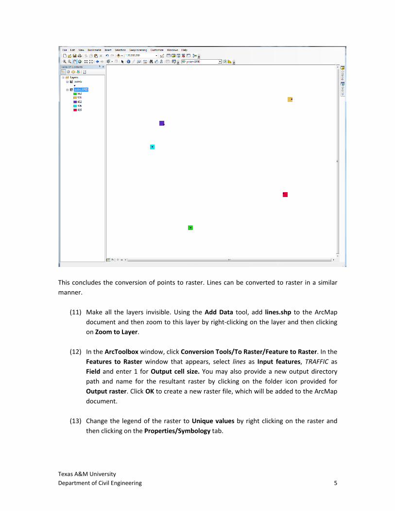
(9) Change the legend of the raster to Unique values by right clicking on the raster and
then by clicking on Properties/Symbology. In the Show window, click Unique Values. (10) Click Yes. Click Apply and then OK in the Layer Properties window.
Note: Submit a layout of the new raster layer.
Texas A&M University Department of Civil Engineering 5
This concludes the conversion of points to raster. Lines can be converted to raster in a similar manner.
(11) Make all the layers invisible. Using the Add Data tool, add lines.shp to the ArcMap document and then zoom to this layer by right-clicking on the layer and then clicking on Zoom to Layer.
(12) In the ArcToolbox window, click Conversion Tools/To Raster/Feature to Raster. In the
Features to Raster window that appears, select lines as Input features, TRAFFIC as Field and enter 1 for Output cell size. You may also provide a new output directory path and name for the resultant raster by clicking on the folder icon provided for Output raster. Click OK to create a new raster file, which will be added to the ArcMap document.
(13) Change the legend of the raster to Unique values by right clicking on the raster and
then clicking on the Properties/Symbology tab.
Texas A&M University Department of Civil Engineering 6
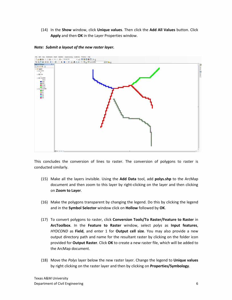
(14) In the Show window, click Unique values. Then click the Add All Values button. Click Apply and then OK in the Layer Properties window.
Note: Submit a layout of the new raster layer.
This concludes the conversion of lines to raster. The conversion of polygons to raster is conducted similarly.
(15) Make all the layers invisible. Using the Add Data tool, add polys.shp to the ArcMap document and then zoom to this layer by right-clicking on the layer and then clicking on Zoom to Layer.
(16) Make the polygons transparent by changing the legend. Do this by clicking the legend
and in the Symbol Selector window click on Hollow followed by OK. (17) To convert polygons to raster, click Conversion Tools/To Raster/Feature to Raster in
ArcToolbox. In the Feature to Raster window, select polys as Input features, HYDCOND as Field, and enter 1 for Output cell size. You may also provide a new output directory path and name for the resultant raster by clicking on the folder icon provided for Output Raster. Click OK to create a new raster file, which will be added to the ArcMap document.
(18) Move the Polys layer below the new raster layer. Change the legend to Unique values
by right clicking on the raster layer and then by clicking on Properties/Symbology.
Texas A&M University Department of Civil Engineering 7
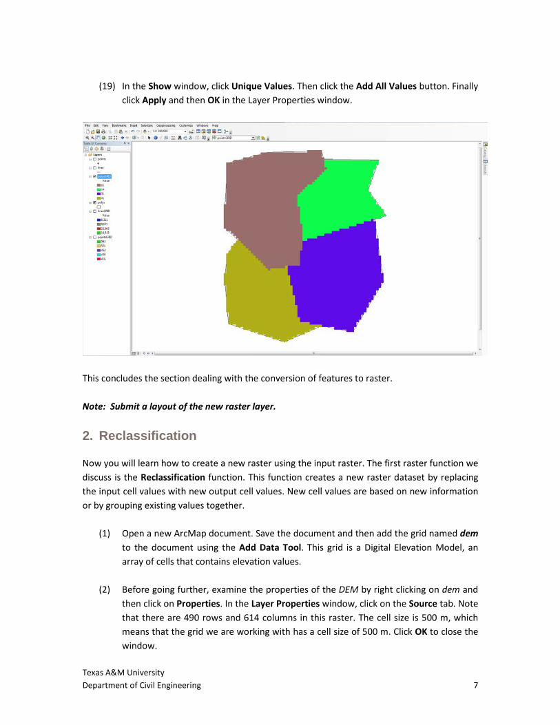
(19) In the Show window, click Unique Values. Then click the Add All Values button. Finally
click Apply and then OK in the Layer Properties window.
This concludes the section dealing with the conversion of features to raster. Note: Submit a layout of the new raster layer.
2. Reclassification Now you will learn how to create a new raster using the input raster. The first raster function we discuss is the Reclassification function. This function creates a new raster dataset by replacing the input cell values with new output cell values. New cell values are based on new information or by grouping existing values together.
(1) Open a new ArcMap document. Save the document and then add the grid named dem to the document using the Add Data Tool. This grid is a Digital Elevation Model, an array of cells that contains elevation values.
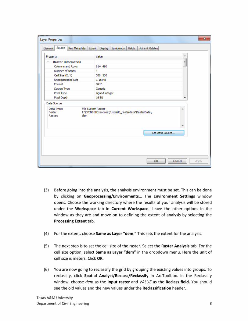
(2) Before going further, examine the properties of the DEM by right clicking on dem and
then click on Properties. In the Layer Properties window, click on the Source tab. Note that there are 490 rows and 614 columns in this raster. The cell size is 500 m, which means that the grid we are working with has a cell size of 500 m. Click OK to close the window.
Texas A&M University Department of Civil Engineering 8
(3) Before going into the analysis, the analysis environment must be set. This can be done
by clicking on Geoprocessing/Environments… The Environment Settings window opens. Choose the working directory where the results of your analysis will be stored under the Workspace tab in Current Workspace. Leave the other options in the window as they are and move on to defining the extent of analysis by selecting the Processing Extent tab.
(4) For the extent, choose Same as Layer “dem.” This sets the extent for the analysis. (5) The next step is to set the cell size of the raster. Select the Raster Analysis tab. For the
cell size option, select Same as Layer “dem” in the dropdown menu. Here the unit of cell size is meters. Click OK.
(6) You are now going to reclassify the grid by grouping the existing values into groups. To reclassify, click Spatial Analyst/Reclass/Reclassify in ArcToolbox. In the Reclassify window, choose dem as the Input raster and VALUE as the Reclass field. You should see the old values and the new values under the Reclassification header.
Texas A&M University Department of Civil Engineering 9
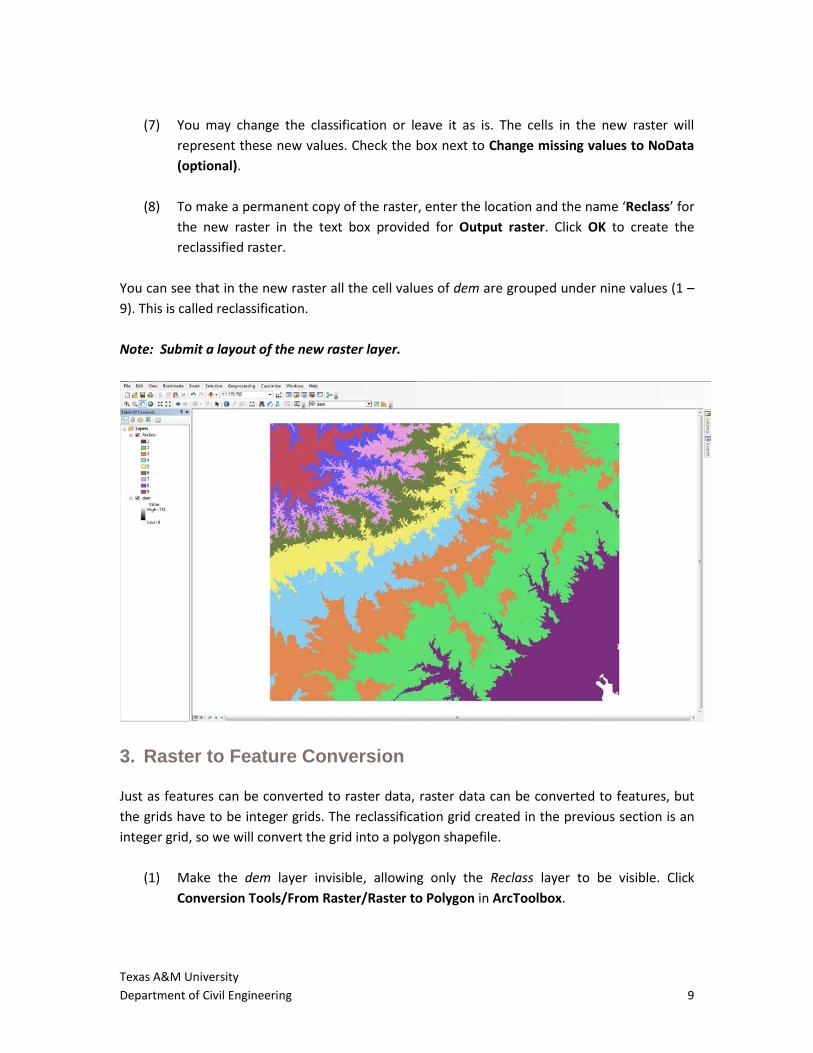
(7) You may change the classification or leave it as is. The cells in the new raster will
represent these new values. Check the box next to Change missing values to NoData (optional).
(8) To make a permanent copy of the raster, enter the location and the name ‘Reclass’ for
the new raster in the text box provided for Output raster. Click OK to create the reclassified raster.
You can see that in the new raster all the cell values of dem are grouped under nine values (1 – 9). This is called reclassification. Note: Submit a layout of the new raster layer.
3. Raster to Feature Conversion Just as features can be converted to raster data, raster data can be converted to features, but the grids have to be integer grids. The reclassification grid created in the previous section is an integer grid, so we will convert the grid into a polygon shapefile.
(1) Make the dem layer invisible, allowing only the Reclass layer to be visible. Click Conversion Tools/From Raster/Raster to Polygon in ArcToolbox.
Texas A&M University Department of Civil Engineering 10
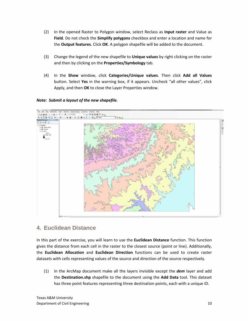
(2) In the opened Raster to Polygon window, select Reclass as Input raster and Value as Field. Do not check the Simplify polygons checkbox and enter a location and name for the Output features. Click OK. A polygon shapefile will be added to the document.
(3) Change the legend of the new shapefile to Unique values by right clicking on the raster
and then by clicking on the Properties/Symbology tab. (4) In the Show window, click Categories/Unique values. Then click Add all Values
button. Select Yes in the warning box, if it appears. Uncheck “all other values”, click Apply, and then OK to close the Layer Properties window.
Note: Submit a layout of the new shapefile.
4. Euclidean Distance In this part of the exercise, you will learn to use the Euclidean Distance function. This function gives the distance from each cell in the raster to the closest source (point or line). Additionally, the Euclidean Allocation and Euclidean Direction functions can be used to create raster datasets with cells representing values of the source and direction of the source respectively.
(1) In the ArcMap document make all the layers invisible except the dem layer and add the Destination.shp shapefile to the document using the Add Data tool. This dataset has three point features representing three destination points, each with a unique ID.
Texas A&M University Department of Civil Engineering 11
(2) To see their IDs, open the attribute table by right clicking on the Destination layer and
then clicking on Open Attribute Table. This ID is important because it is useful when the allocation is defined for the cells. Close the attribute table.
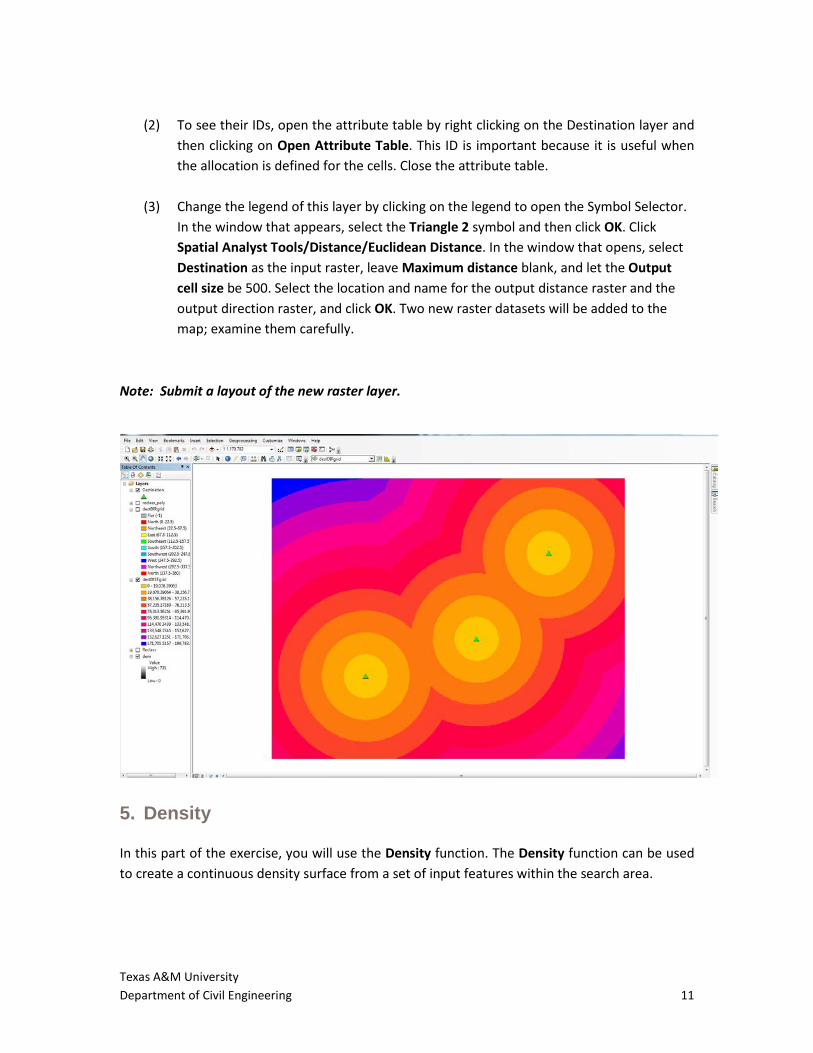
(3) Change the legend of this layer by clicking on the legend to open the Symbol Selector.
In the window that appears, select the Triangle 2 symbol and then click OK. Click Spatial Analyst Tools/Distance/Euclidean Distance. In the window that opens, select Destination as the input raster, leave Maximum distance blank, and let the Output cell size be 500. Select the location and name for the output distance raster and the output direction raster, and click OK. Two new raster datasets will be added to the map; examine them carefully.
Note: Submit a layout of the new raster layer.
5. Density In this part of the exercise, you will use the Density function. The Density function can be used to create a continuous density surface from a set of input features within the search area.
Texas A&M University Department of Civil Engineering 12
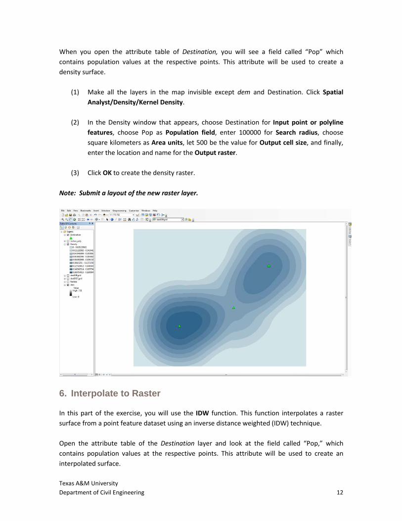
When you open the attribute table of Destination, you will see a field called “Pop” which contains population values at the respective points. This attribute will be used to create a density surface.
(1) Make all the layers in the map invisible except dem and Destination. Click Spatial Analyst/Density/Kernel Density.
(2) In the Density window that appears, choose Destination for Input point or polyline
features, choose Pop as Population field, enter 100000 for Search radius, choose square kilometers as Area units, let 500 be the value for Output cell size, and finally, enter the location and name for the Output raster.
(3) Click OK to create the density raster.
Note: Submit a layout of the new raster layer.
6. Interpolate to Raster In this part of the exercise, you will use the IDW function. This function interpolates a raster surface from a point feature dataset using an inverse distance weighted (IDW) technique. Open the attribute table of the Destination layer and look at the field called “Pop,” which contains population values at the respective points. This attribute will be used to create an interpolated surface.
Texas A&M University Department of Civil Engineering 13
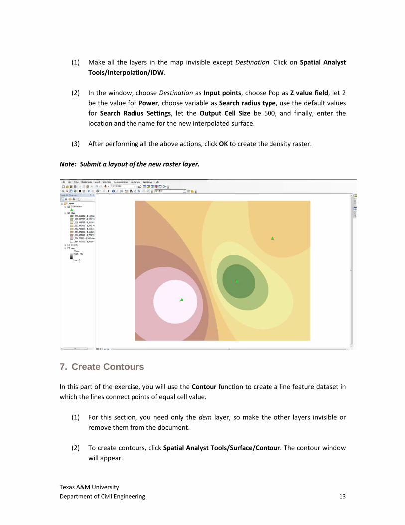
(1) Make all the layers in the map invisible except Destination. Click on Spatial Analyst
Tools/Interpolation/IDW. (2) In the window, choose Destination as Input points, choose Pop as Z value field, let 2
be the value for Power, choose variable as Search radius type, use the default values for Search Radius Settings, let the Output Cell Size be 500, and finally, enter the location and the name for the new interpolated surface.
(3) After performing all the above actions, click OK to create the density raster.
Note: Submit a layout of the new raster layer.
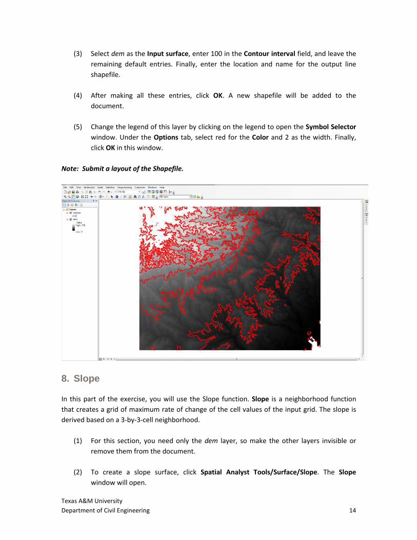
7. Create Contours In this part of the exercise, you will use the Contour function to create a line feature dataset in which the lines connect points of equal cell value.
(1) For this section, you need only the dem layer, so make the other layers invisible or remove them from the document.
(2) To create contours, click Spatial Analyst Tools/Surface/Contour. The contour window
will appear.
Texas A&M University Department of Civil Engineering 14
(3) Select dem as the Input surface, enter 100 in the Contour interval field, and leave the remaining default entries. Finally, enter the location and name for the output line shapefile.
(4) After making all these entries, click OK. A new shapefile will be added to the
document. (5) Change the legend of this layer by clicking on the legend to open the Symbol Selector
window. Under the Options tab, select red for the Color and 2 as the width. Finally, click OK in this window.
Note: Submit a layout of the Shapefile.
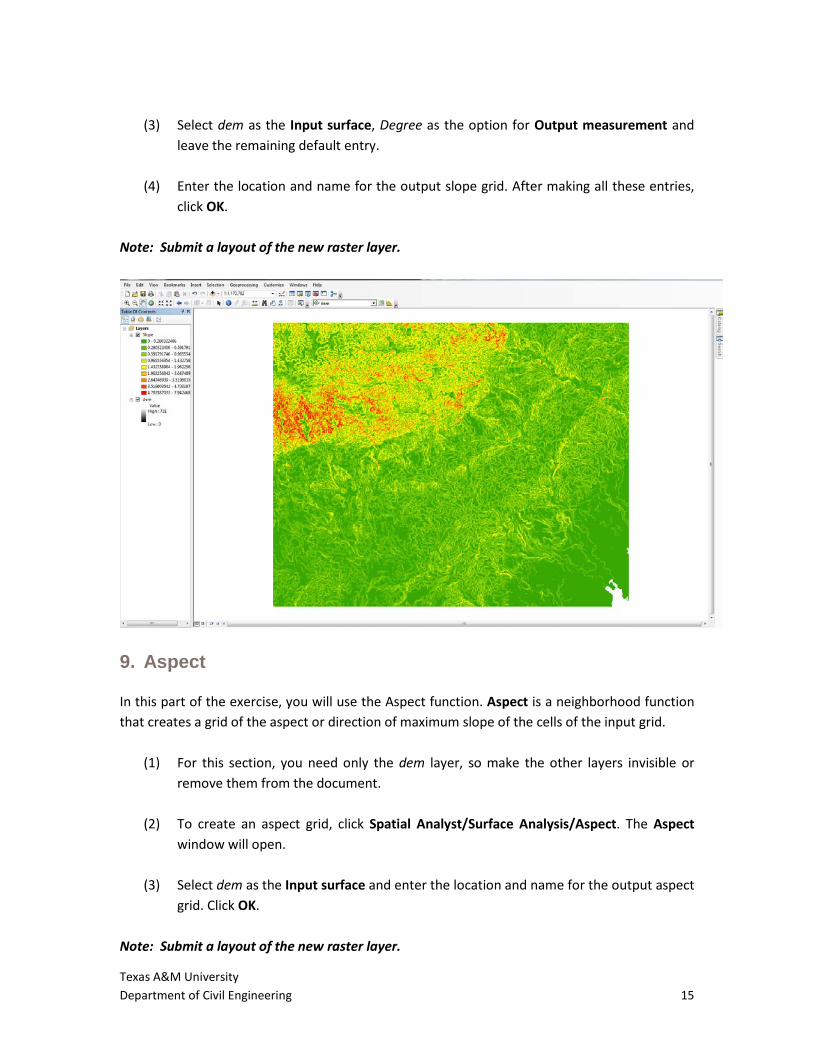
8. Slope In this part of the exercise, you will use the Slope function. Slope is a neighborhood function that creates a grid of maximum rate of change of the cell values of the input grid. The slope is derived based on a 3-by-3-cell neighborhood.
(1) For this section, you need only the dem layer, so make the other layers invisible or remove them from the document.
(2) To create a slope surface, click Spatial Analyst Tools/Surface/Slope. The Slope
window will open.
Texas A&M University Department of Civil Engineering 15
(3) Select dem as the Input surface, Degree as the option for Output measurement and
leave the remaining default entry. (4) Enter the location and name for the output slope grid. After making all these entries,
click OK. Note: Submit a layout of the new raster layer.
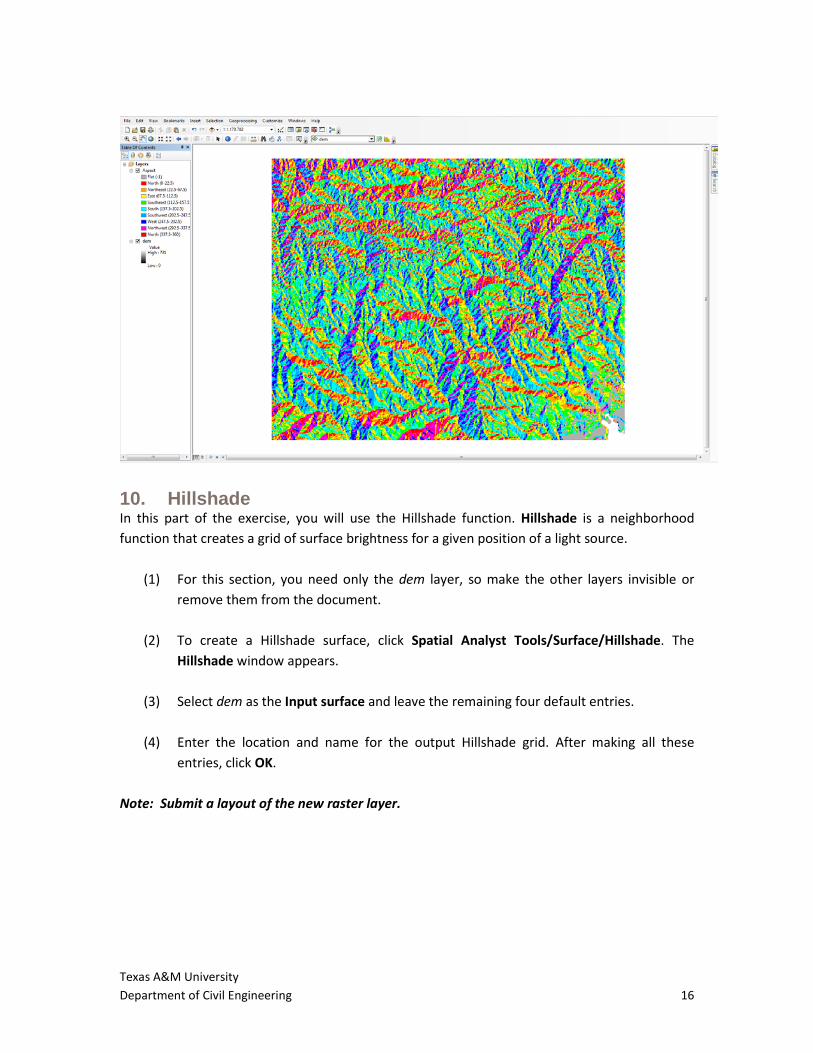
9. Aspect In this part of the exercise, you will use the Aspect function. Aspect is a neighborhood function that creates a grid of the aspect or direction of maximum slope of the cells of the input grid.
(1) For this section, you need only the dem layer, so make the other layers invisible or remove them from the document.
(2) To create an aspect grid, click Spatial Analyst/Surface Analysis/Aspect. The Aspect
window will open. (3) Select dem as the Input surface and enter the location and name for the output aspect
grid. Click OK. Note: Submit a layout of the new raster layer.
Texas A&M University Department of Civil Engineering 16
10. Hillshade In this part of the exercise, you will use the Hillshade function. Hillshade is a neighborhood function that creates a grid of surface brightness for a given position of a light source.
(1) For this section, you need only the dem layer, so make the other layers invisible or remove them from the document.
(2) To create a Hillshade surface, click Spatial Analyst Tools/Surface/Hillshade. The
Hillshade window appears. (3) Select dem as the Input surface and leave the remaining four default entries. (4) Enter the location and name for the output Hillshade grid. After making all these
entries, click OK. Note: Submit a layout of the new raster layer.
Texas A&M University Department of Civil Engineering 17
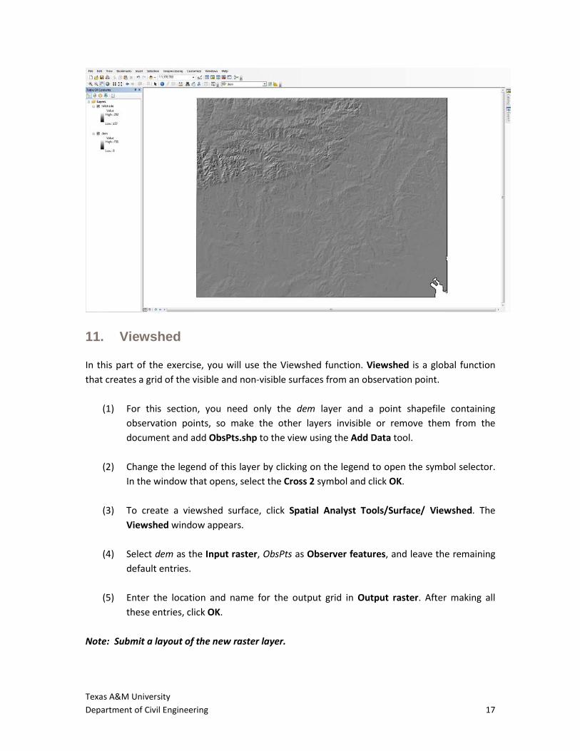
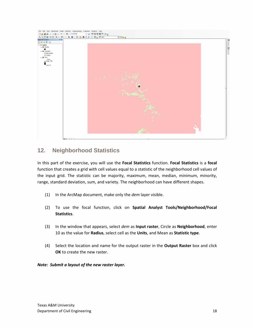
11. Viewshed In this part of the exercise, you will use the Viewshed function. Viewshed is a global function that creates a grid of the visible and non-visible surfaces from an observation point.
(1) For this section, you need only the dem layer and a point shapefile containing observation points, so make the other layers invisible or remove them from the document and add ObsPts.shp to the view using the Add Data tool.
(2) Change the legend of this layer by clicking on the legend to open the symbol selector.
In the window that opens, select the Cross 2 symbol and click OK. (3) To create a viewshed surface, click Spatial Analyst Tools/Surface/ Viewshed. The
Viewshed window appears. (4) Select dem as the Input raster, ObsPts as Observer features, and leave the remaining
default entries. (5) Enter the location and name for the output grid in Output raster. After making all
these entries, click OK. Note: Submit a layout of the new raster layer.
Texas A&M University Department of Civil Engineering 18
12. Neighborhood Statistics In this part of the exercise, you will use the Focal Statistics function. Focal Statistics is a focal function that creates a grid with cell values equal to a statistic of the neighborhood cell values of the input grid. The statistic can be majority, maximum, mean, median, minimum, minority, range, standard deviation, sum, and variety. The neighborhood can have different shapes.
(1) In the ArcMap document, make only the dem layer visible. (2) To use the focal function, click on Spatial Analyst Tools/Neighborhood/Focal
Statistics. (3) In the window that appears, select dem as Input raster, Circle as Neighborhood, enter
10 as the value for Radius, select cell as the Units, and Mean as Statistic type. (4) Select the location and name for the output raster in the Output Raster box and click
OK to create the new raster. Note: Submit a layout of the new raster layer.
Texas A&M University Department of Civil Engineering 19
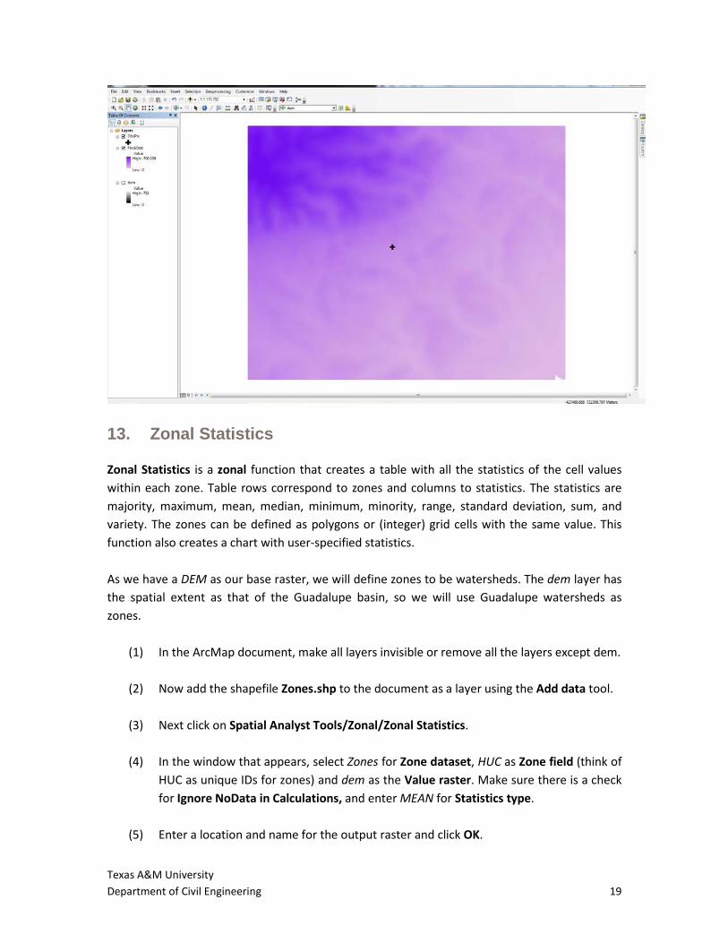
13. Zonal Statistics Zonal Statistics is a zonal function that creates a table with all the statistics of the cell values within each zone. Table rows correspond to zones and columns to statistics. The statistics are majority, maximum, mean, median, minimum, minority, range, standard deviation, sum, and variety. The zones can be defined as polygons or (integer) grid cells with the same value. This function also creates a chart with user-specified statistics. As we have a DEM as our base raster, we will define zones to be watersheds. The dem layer has the spatial extent as that of the Guadalupe basin, so we will use Guadalupe watersheds as zones.
(1) In the ArcMap document, make all layers invisible or remove all the layers except dem. (2) Now add the shapefile Zones.shp to the document as a layer using the Add data tool. (3) Next click on Spatial Analyst Tools/Zonal/Zonal Statistics. (4) In the window that appears, select Zones for Zone dataset, HUC as Zone field (think of
HUC as unique IDs for zones) and dem as the Value raster. Make sure there is a check for Ignore NoData in Calculations, and enter MEAN for Statistics type.
(5) Enter a location and name for the output raster and click OK.
Texas A&M University Department of Civil Engineering 20
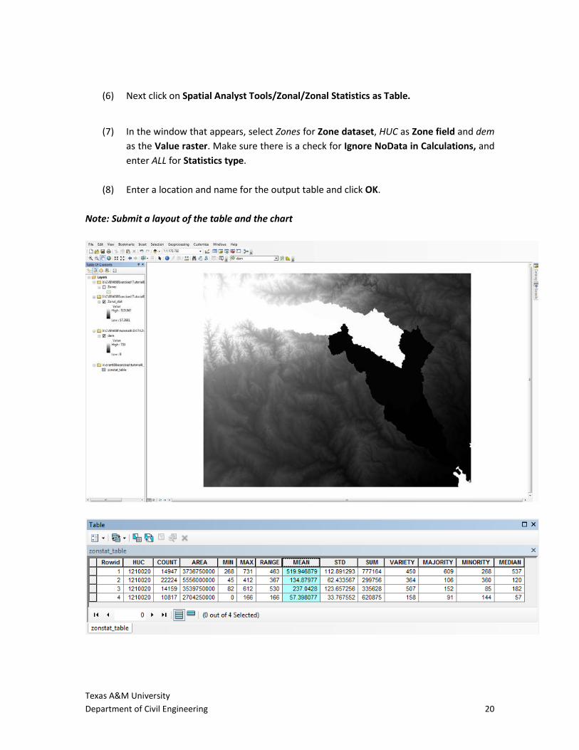
(6) Next click on Spatial Analyst Tools/Zonal/Zonal Statistics as Table.
(7) In the window that appears, select Zones for Zone dataset, HUC as Zone field and dem as the Value raster. Make sure there is a check for Ignore NoData in Calculations, and enter ALL for Statistics type.
(8) Enter a location and name for the output table and click OK.
Note: Submit a layout of the table and the chart
Texas A&M University Department of Civil Engineering 21
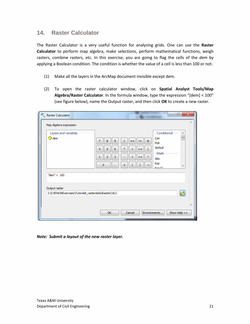
14. Raster Calculator The Raster Calculator is a very useful function for analyzing grids. One can use the Raster Calculator to perform map algebra, make selections, perform mathematical functions, weigh rasters, combine rasters, etc. In this exercise, you are going to flag the cells of the dem by applying a Boolean condition. The condition is whether the value of a cell is less than 100 or not.
(1) Make all the layers in the ArcMap document invisible except dem. (2) To open the raster calculator window, click on Spatial Analyst Tools/Map
Algebra/Raster Calculator. In the formula window, type the expression “[dem] < 100” (see figure below), name the Output raster, and then click OK to create a new raster.
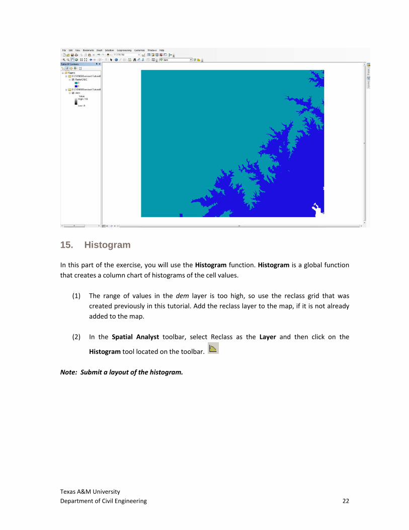
Note: Submit a layout of the new raster layer.
Texas A&M University Department of Civil Engineering 22
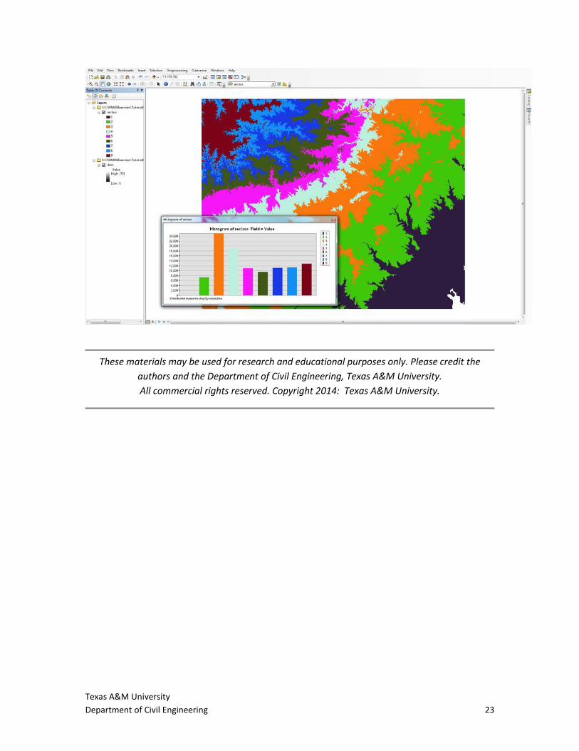
15. Histogram In this part of the exercise, you will use the Histogram function. Histogram is a global function that creates a column chart of histograms of the cell values.
(1) The range of values in the dem layer is too high, so use the reclass grid that was created previously in this tutorial. Add the reclass layer to the map, if it is not already added to the map.
(2) In the Spatial Analyst toolbar, select Reclass as the Layer and then click on the
Histogram tool located on the toolbar. Note: Submit a layout of the histogram.
Texas A&M University Department of Civil Engineering 23
These materials may be used for research and educational purposes only. Please credit the
authors and the Department of Civil Engineering, Texas A&M University. All commercial rights reserved. Copyright 2014: Texas A&M University.