Embed Size (px)
Citation preview
2008 ESRI International User Conference
1
Spatial and Temporal Analysis of Urban Traffic Volume
Changjoo Kima, Yong-seuk Parkb, and Sunhee Sangc
a Department of Geography, University of Cincinnati, 401D Braunstein Hall,
Cincinnati, OH 45221, USA b Department of Geography, Minnesota State University, 7 Armstrong Hall,
Mankato, MN 56001, USA c Department of Geography, The Ohio State University, 1036 Derby Hall, 154 N. Oval Mall,
Columbus, OH 43210, USA
Abstract
This study explores traffic patterns in the Twin Cities metropolitan area from 1997 to 2006.
Traffic flows are analyzed at the annual, monthly, weekly, and daily time scale. The results
show that there are significant traffic volume changes among 847 traffic volume count stations in
major highways with respect to temporary and spatial aspects. For the ten years, the annual total
traffic volume has been increased. However, the increase rate of traffic volume has been
decreased since 2004. The study illustrates that the new public transit (LRT) helps decrease the
urban traffic volume on the major highways. In terms of the monthly traffic volume pattern,
August has the highest traffic volume whereas January has the lowest traffic volume. The
difference in monthly fluctuation is mainly due to weather conditions. Among the days of week,
Friday has the most traffic volume whereas Sunday has the least. Commuting traffic flows are
used to illustrate the hourly traffic pattern.
Key words: transportation, GIS, traffic volume, commute, light-rail train, the drive miles per
vehicle
1 Introduction
Based on previous studies regarding urban traffic flow, there are several common
findings. First, urban traffic volume is increasing every year. Second, studies show that urban
traffic problems occur due to over-supplied traffic on limited roadways. Third, traffic congestion
is not incurred randomly. Fourth, traffic volume pattern is different spatially and temporary.
2008 ESRI International User Conference
2
Last, a deep understanding of traffic flow gives benefits to all levels of government and private
agencies.
In the U.S., traffic volume has been increasing rapidly especially in the metropolitan
areas, likewise a total number of vehicle miles on all roads and streets have been increasing as
well. According to the traffic volume trend report from the Federal Highway Administration
(FHWA), the number of annual vehicle distance traveled on roads has doubled compared to the
value in the year 1981. In addition, FHWA estimated that an individual driver drove 1,036
vehicle miles (35%) in rural areas and 1,960 miles (65%) in urban areas in 2006 (FHWA, Traffic
Volume Trend 2007). However, road infrastructure has not increased as much as demand
increased. A total distance of lane in the U.S. has increased 2.62 percent: the total distance of
lane is 8,158,181 miles in 1995 whereas it is 8,371,718 miles in 2005 (FHWA, Highway
Statistics 1995 1995, FHWA, Highway Statistics 2005 2006). These reports imply that overall
traffic volume has increased greatly in the U.S., a high percent of the traffic volume is related
with urban area, and supplied infrastructure does not meet the traffic demands. As traffic
volume increases in an urban area, urban traffic congestion becomes a serious problem. Cervero
(2006) addressed that traffic congestion incurs not only waste time, money, and energy but also
affects productivity. In terms of monetary loss, in 2002, the traffic congestion wasted 63.2
billion dollars in urbanized areas of North America (Schrank and Lomax. 2004).
Contemporary traffic data collection became the responsibility of State DOTs, cities,
counties, metropolitan planning organizations in standard rule (Mergel 1997). For example, the
Minnesota Department of Transportation (MN DOT) has been collecting and forecasting traffic
volume statewide using the Traffic Monitoring Guide by FHWA. MN DOT uses two different
data frameworks; one is for short duration counts, and another is for permanent continuous
counts. These frameworks use three detectors, such as the Automated Traffic Recorder, Weigh
in Motion, and Tube Counters to count traffic flow. Based on the collected traffic flow
information, MN DOT provides various information of traffic flow such as Average Annual
Daily Traffic (or “AADT”), Average Daily Traffic (or “ADT”), Average Daily Load (or “ADL”),
Average Summer Weekly Traffic (or “ASWDT”), Heavy Commercial Annual Average Daily
Traffic (or “HCAADT”), etc. Therefore, transportation practitioners and researchers can
articulate their research via the mobility of human and accessibility of location in order to find
and solve derivative problems of urbanization. The short duration and continuous traffic count
2008 ESRI International User Conference
3
are related with capabilities of transportation infrastructures such as road facilities, parking lots,
public transportation systems, etc. These capabilities of transportation infrastructures are related
with receptive capability of living environmental capacity such as noise level, air quality,
commuting time, traffic congestion, etc.
A travel pattern model consists of home, workplace, day care center, food store, and
health club as aspects of daily travel pattern (Hanson 2004). Among these trips, journey to work
is the most important factor of urban traffic flow. In 1983, FHWA estimated that 30.7 percent of
vehicle-trips are related with work or work related business purposes: 20 percent with shopping,
1.2 percent for health, 14.9 percent for family related, 5.9 percent for school or religion, 22.2
percent for all social and recreation including vacation, visit friends, pleasure driving, etc.
(FHWA, America's Challenge for highway transportation in the 21st century 1988). Thus, the
research concluded that commuting flow is the highest proportion of overall urban traffic flow.
The drive alone percentage is relatively higher than any other modes; also it has increased
gradually (Nancy and Nanda 2003). This implies that the number of people driving to work
alone is almost as high as the total commuter traffic flow.
2 Background
The Twin Cities metropolitan area consists of seven counties: Anoka, Carver, Dakota,
Hennepin, Ramsey, Scott and Washington. When looking at size, economy, employment and
education, the Metropolitan Area has a great influence on the Midwestern United States.
According to the U.S. Census Bureau, the population of the area is approximately 2.64 million as
of 2000. The Twin Cities metro area is ranked 15th in population the 25 major metropolitan
areas in the U.S. Regarding the economy, the metro area is considered as one of the economical
hotspots in the Midwest. As of 2007, 32 of the Fortune 1000 companies are headquartered in the
Twin Cities Metro Area (Tully 2007). In terms of the average median family income ($54,304)
and household income ($65,450), the metropolitan area is ranked as the 3rd highest out of the 25
major metro areas in the U.S. The poverty rate is ranked the least as the 25th. As aspect of work
force, the rate of labor force participation is high when compared to other metro areas. It is
ranked as the highest at 74.3 percent. The unemployment rate is relatively low. In terms of
education levels of workforce, more than 90 percent of the residents have at least a high school
diploma, and more than 33 percent of the residents have a bachelor’s degree or higher.
2008 ESRI International User Conference
4
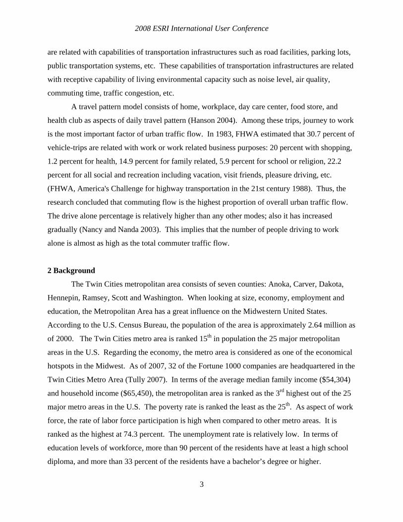
In terms of the transportation system, there is air transportation service and two major public
transportation services such as light rail and bus. Regarding air transportation service, there is
the Minneapolis-Saint Paul International Airport (MSP) which is the busiest airport among the
upper Midwest region. It serves as a main hub for Northwest Airlines, Sun Country Airlines,
and Champion Airlines. In regards to public transit, there are 198 bus routes and one light rail
service. The bus routes mainly cover the downtown area, and the light rail route covers from
downtown Minneapolis – Minneapolis – Fort Snelling – MSP - Mall of America. There are
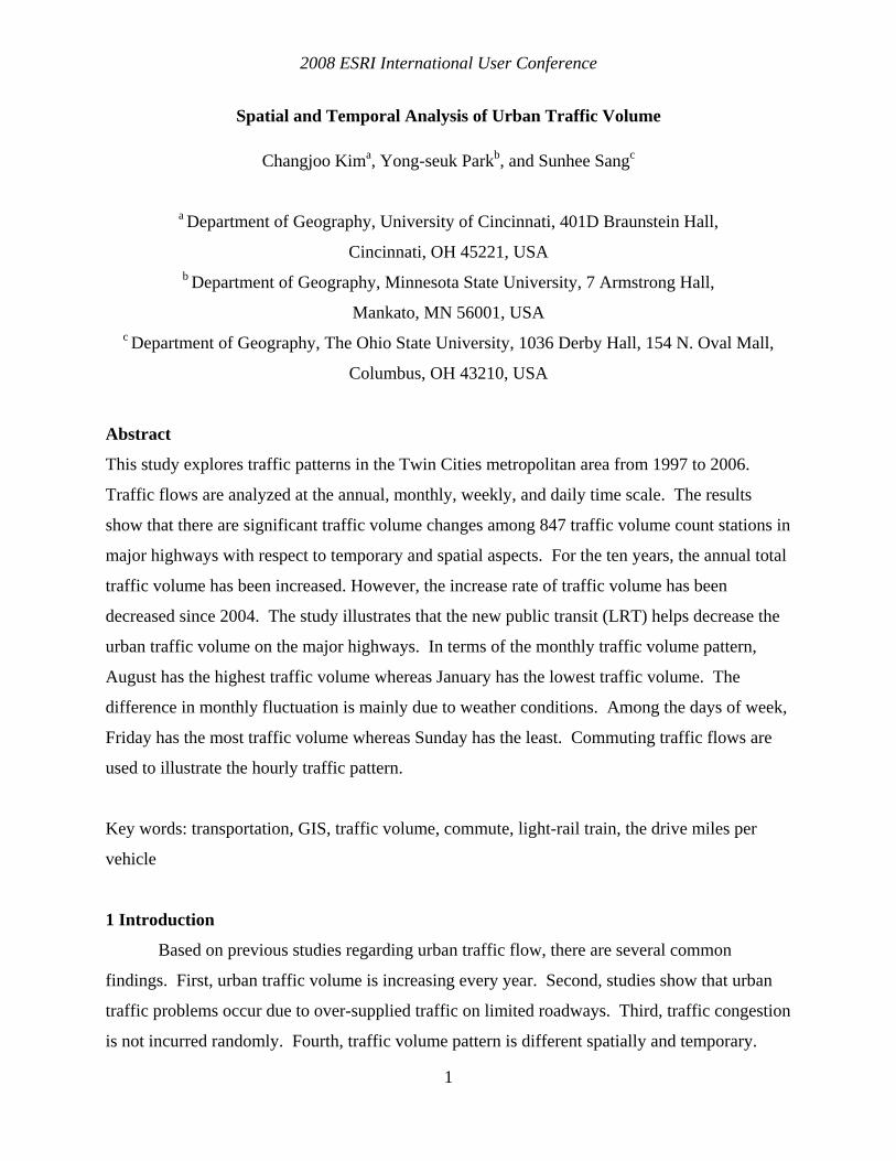
three major highway systems around the Twin Cities metropolitan area. Seven interstate
highways run throughout the area: I-35, I-35 East, I-35 West, I-94, I-394, I-494 and I-694. The
traffic volume data has been continuously collected by MN DOT since 1997 over the 847
stations on the major highways. Each station consists of several detectors which count traffic
volume at 30 second intervals. In terms of efficiency of data handling and a common agreement
of data aggregation level, the traffic volume is aggregated to 60 minute intervals in this study.
Figure 1. Study Area: The Twin Cities Metropolitan Area
o
Hennepin
Dakota
Scott
Washington
Anoka
Ramsey
Carver
MSP
0 4 82 Miles
±
o msp
STATION
Hiawatha Corridor Light Rail Line Alignment
Mojor Highways
sevenCounty
2008 ESRI International User Conference
5
3 Temporal Traffic Patterns
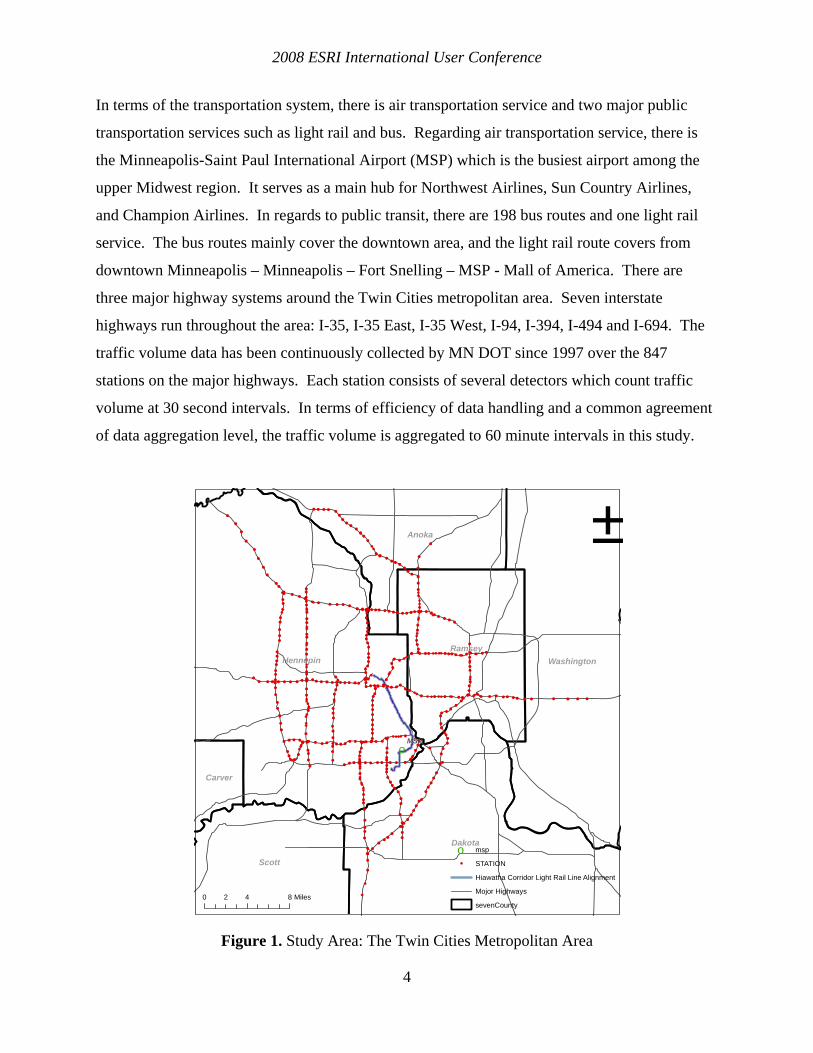
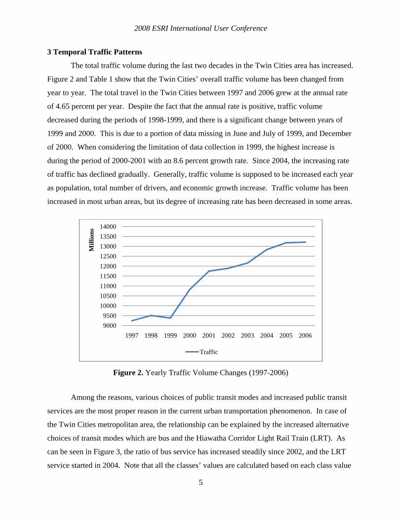
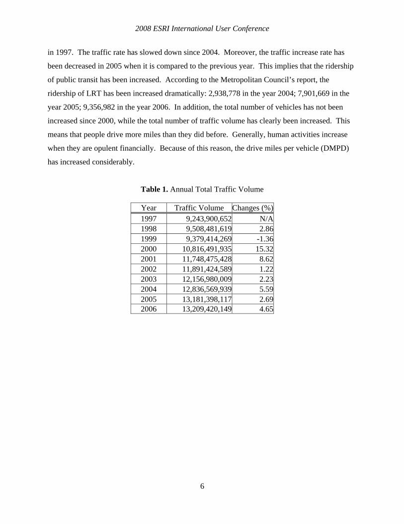
The total traffic volume during the last two decades in the Twin Cities area has increased.
Figure 2 and Table 1 show that the Twin Cities’ overall traffic volume has been changed from
year to year. The total travel in the Twin Cities between 1997 and 2006 grew at the annual rate
of 4.65 percent per year. Despite the fact that the annual rate is positive, traffic volume
decreased during the periods of 1998-1999, and there is a significant change between years of
1999 and 2000. This is due to a portion of data missing in June and July of 1999, and December
of 2000. When considering the limitation of data collection in 1999, the highest increase is
during the period of 2000-2001 with an 8.6 percent growth rate. Since 2004, the increasing rate
of traffic has declined gradually. Generally, traffic volume is supposed to be increased each year
as population, total number of drivers, and economic growth increase. Traffic volume has been
increased in most urban areas, but its degree of increasing rate has been decreased in some areas.
Figure 2. Yearly Traffic Volume Changes (1997-2006)
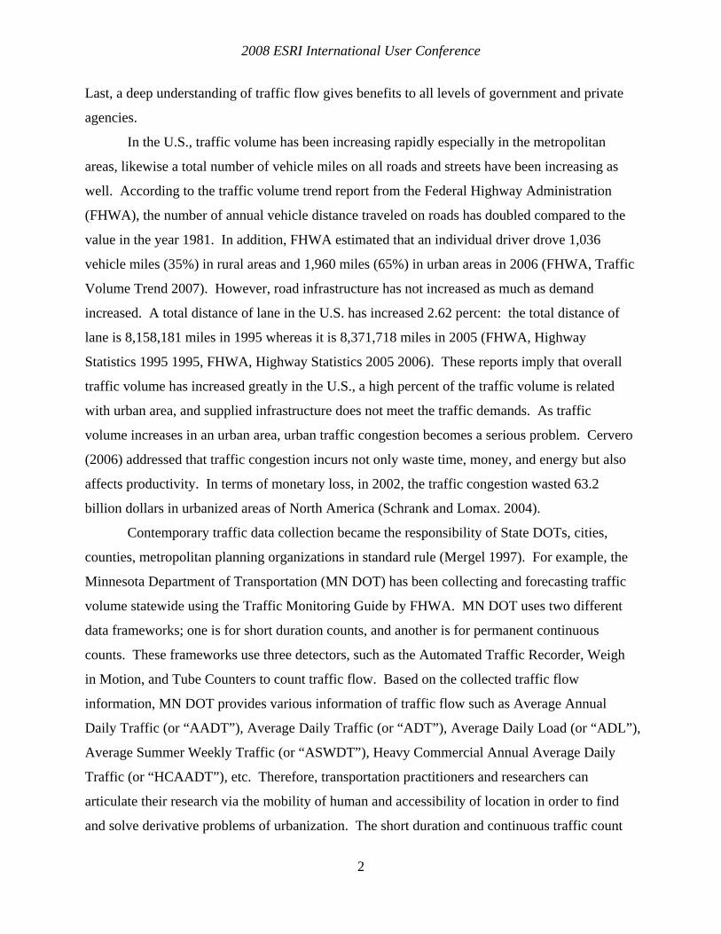
Among the reasons, various choices of public transit modes and increased public transit
services are the most proper reason in the current urban transportation phenomenon. In case of
the Twin Cities metropolitan area, the relationship can be explained by the increased alternative
choices of transit modes which are bus and the Hiawatha Corridor Light Rail Train (LRT). As
can be seen in Figure 3, the ratio of bus service has increased steadily since 2002, and the LRT
service started in 2004. Note that all the classes’ values are calculated based on each class value
90009500
100001050011000115001200012500130001350014000
1997 1998 1999 2000 2001 2002 2003 2004 2005 2006
Mill
ions
Traffic
2008 ESRI International User Conference
6
in 1997. The traffic rate has slowed down since 2004. Moreover, the traffic increase rate has
been decreased in 2005 when it is compared to the previous year. This implies that the ridership
of public transit has been increased. According to the Metropolitan Council’s report, the
ridership of LRT has been increased dramatically: 2,938,778 in the year 2004; 7,901,669 in the
year 2005; 9,356,982 in the year 2006. In addition, the total number of vehicles has not been
increased since 2000, while the total number of traffic volume has clearly been increased. This
means that people drive more miles than they did before. Generally, human activities increase
when they are opulent financially. Because of this reason, the drive miles per vehicle (DMPD)
has increased considerably.
Table 1. Annual Total Traffic Volume
Year Traffic Volume Changes (%)1997 9,243,900,652 N/A1998 9,508,481,619 2.861999 9,379,414,269 -1.362000 10,816,491,935 15.322001 11,748,475,428 8.622002 11,891,424,589 1.222003 12,156,980,009 2.232004 12,836,569,939 5.592005 13,181,398,117 2.692006 13,209,420,149 4.65

2008 ESRI International User Conference
7
Figure 3. Comparison: Traffic volume, GDP, Number of vehicles and licenses
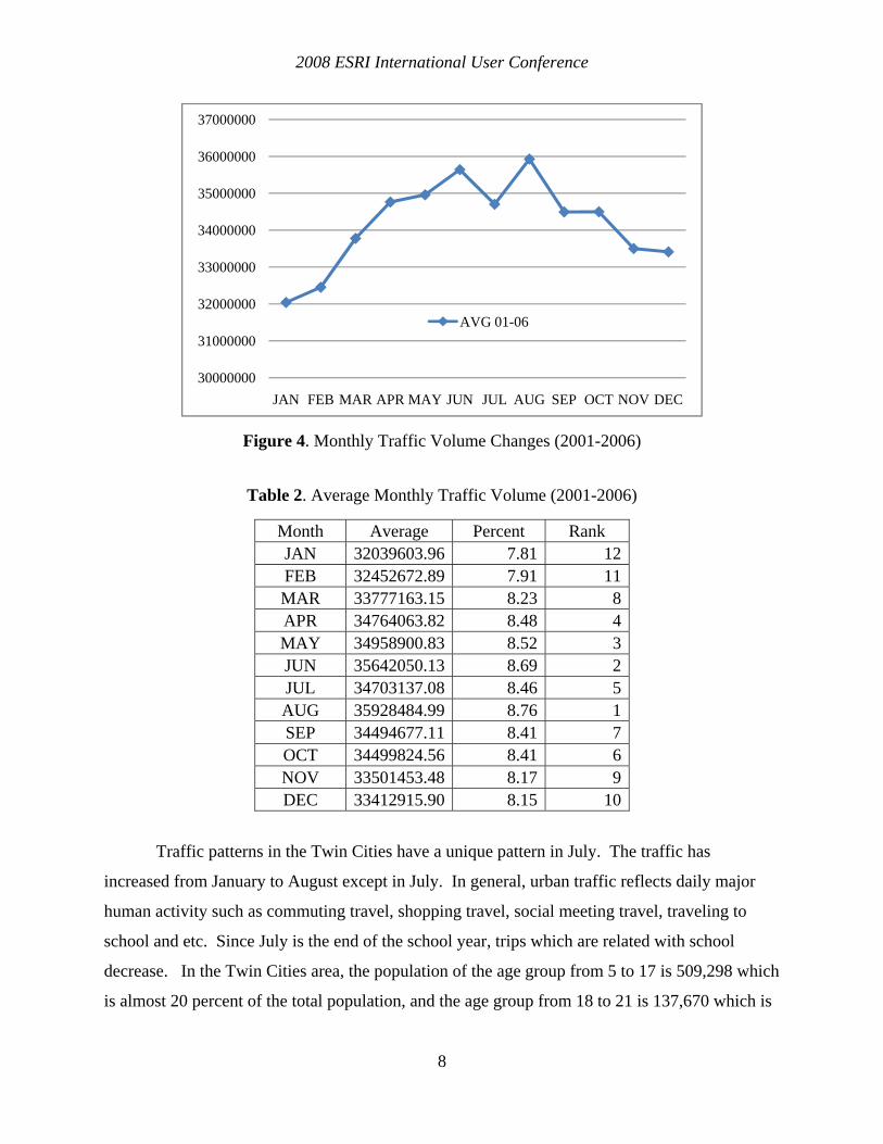
Figure 4 and Table 2 show the general traffic volume pattern from month-to-month. In
order to represent the most recent trend, the average total traffic volume between 2001 and 2006
is shown. The chart and table represent the average daily total traffic volume for each month
during the periods from 2001 to 2006. This is calculated by dividing the monthly total amount of
traffic volume for each month by the number of days in each month. As can be seen in Figure 4,
January has the lowest traffic, whereas August has the highest. The average traffic volume has
increased from January to June steadily then it drops off in July. After August it decreases until
January. The peak month and low point trend match and coincide with the nation-wide traffic
pattern. Festin (1996) previously showed the similar results where the peak month for traffic
volume in the U.S. is August, and the lowest level of traffic occurs in January. He also
addressed that the traffic pattern is different between rural and urban areas. Traffic in rural areas
has more seasonal variation than traffic in urban areas. The reason is that summer traffic in rural
areas involves more seasonal vacation or tourism traffic volume. The gap in the Twin Cities
metropolitan area is less than 10 percent like traffic in other urban areas. Generally, traffic
volume in the winter season appears lower than other seasons.
0.90
1.00
1.10
1.20
1.30
1.40
1.50
1.60
1.70
Incr
ease
Rat
e
INDEX_TRAFFICINDEX_VEHICLESINDEX_AUTO
INDEX_BUS
INDEX_TRUCK
2008 ESRI International User Conference
8
Figure 4. Monthly Traffic Volume Changes (2001-2006)
Table 2. Average Monthly Traffic Volume (2001-2006)
Month Average Percent Rank JAN 32039603.96 7.81 12 FEB 32452672.89 7.91 11 MAR 33777163.15 8.23 8 APR 34764063.82 8.48 4 MAY 34958900.83 8.52 3 JUN 35642050.13 8.69 2 JUL 34703137.08 8.46 5 AUG 35928484.99 8.76 1 SEP 34494677.11 8.41 7 OCT 34499824.56 8.41 6 NOV 33501453.48 8.17 9 DEC 33412915.90 8.15 10
Traffic patterns in the Twin Cities have a unique pattern in July. The traffic has
increased from January to August except in July. In general, urban traffic reflects daily major
human activity such as commuting travel, shopping travel, social meeting travel, traveling to
school and etc. Since July is the end of the school year, trips which are related with school
decrease. In the Twin Cities area, the population of the age group from 5 to 17 is 509,298 which
is almost 20 percent of the total population, and the age group from 18 to 21 is 137,670 which is
30000000
31000000
32000000
33000000
34000000
35000000
36000000
37000000
JAN FEB MAR APR MAY JUN JUL AUG SEP OCT NOV DEC
AVG 01-06
2008 ESRI International User Conference
9
almost 5 percent of the total population respectively. Therefore, in terms of school’s summer
break, traffic volume may decrease in July.
In the Twin Cities metropolitan area, traffic volume in the winter season (November –
February) is relatively lower than traffic in other seasons. The average traffic volume in the
winter season is 0.5 percent lower than average of other seasons (Table 2). On average, ground
is covered by at least 1 inch of snow for more than 100 days in between November 22nd and the
next year of April 2nd (MPX 2006). The snowing and low temperature conditions lead elderly
seasonal migration from Minnesota to the Sunbelt States such as Arizona, California, Florida or
Texas. Hogan and Steinnes (1994) addressed that over 20 percent of the seasonal migrants from
Minnesota start the activity before the age of 60, and the elderly seasonal migration rate in the
area is 10.1 percent. In the Twin Cities Metro Area there is of population of 365,837 in the 50 to
64 age range and 255,245 in the 65 and above range. Collectively, these age groups represent 24%
of the total Metro Area population (US Census Bureau, 2000). Therefore, during the winter
season, roughly, 62,108 people are not residing in the area. The number of seasonal migrants
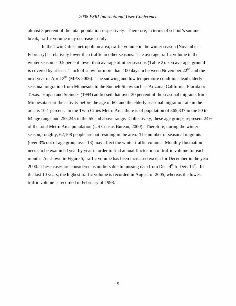
(over 3% out of age group over 18) may affect the winter traffic volume. Monthly fluctuation
needs to be examined year by year in order to find annual fluctuation of traffic volume for each
month. As shown in Figure 5, traffic volume has been increased except for December in the year
2000. These cases are considered as outliers due to missing data from Dec. 4th to Dec. 14th. In
the last 10 years, the highest traffic volume is recorded in August of 2005, whereas the lowest
traffic volume is recorded in February of 1998.
2008 ESRI International User Conference
10
Figure 5. Daily Total Traffic Volume Changes by Month (1997-2006)
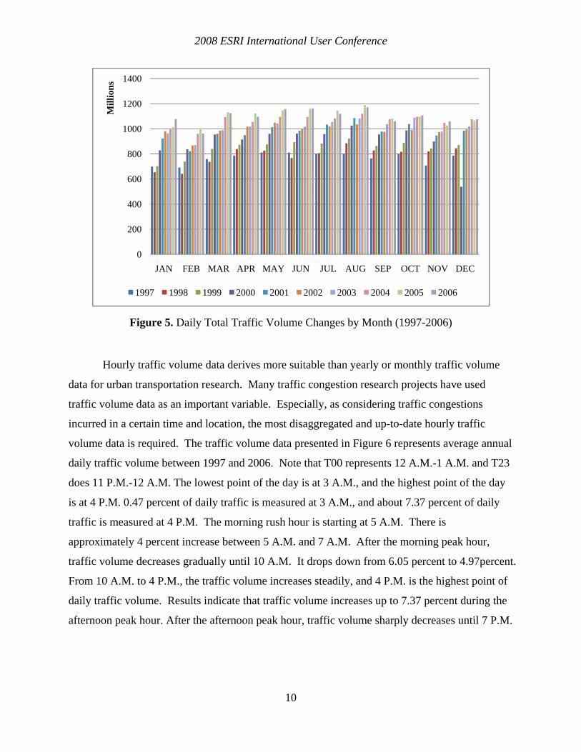
Hourly traffic volume data derives more suitable than yearly or monthly traffic volume
data for urban transportation research. Many traffic congestion research projects have used
traffic volume data as an important variable. Especially, as considering traffic congestions
incurred in a certain time and location, the most disaggregated and up-to-date hourly traffic
volume data is required. The traffic volume data presented in Figure 6 represents average annual
daily traffic volume between 1997 and 2006. Note that T00 represents 12 A.M.-1 A.M. and T23
does 11 P.M.-12 A.M. The lowest point of the day is at 3 A.M., and the highest point of the day
is at 4 P.M. 0.47 percent of daily traffic is measured at 3 A.M., and about 7.37 percent of daily
traffic is measured at 4 P.M. The morning rush hour is starting at 5 A.M. There is
approximately 4 percent increase between 5 A.M. and 7 A.M. After the morning peak hour,
traffic volume decreases gradually until 10 A.M. It drops down from 6.05 percent to 4.97percent.
From 10 A.M. to 4 P.M., the traffic volume increases steadily, and 4 P.M. is the highest point of
daily traffic volume. Results indicate that traffic volume increases up to 7.37 percent during the
afternoon peak hour. After the afternoon peak hour, traffic volume sharply decreases until 7 P.M.
0
200
400
600
800
1000
1200
1400
JAN FEB MAR APR MAY JUN JUL AUG SEP OCT NOV DEC
Mill
ions
1997 1998 1999 2000 2001 2002 2003 2004 2005 2006
2008 ESRI International User Conference
11
Figure 6. Distribution of Average Annual Daily Traffic (1996-2006)
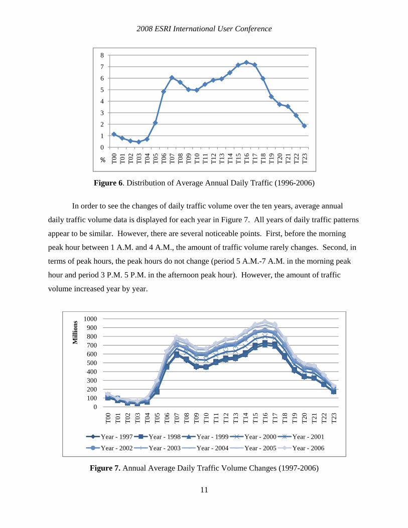
In order to see the changes of daily traffic volume over the ten years, average annual
daily traffic volume data is displayed for each year in Figure 7. All years of daily traffic patterns
appear to be similar. However, there are several noticeable points. First, before the morning
peak hour between 1 A.M. and 4 A.M., the amount of traffic volume rarely changes. Second, in
terms of peak hours, the peak hours do not change (period 5 A.M.-7 A.M. in the morning peak
hour and period 3 P.M. 5 P.M. in the afternoon peak hour). However, the amount of traffic
volume increased year by year.
Figure 7. Annual Average Daily Traffic Volume Changes (1997-2006)
0
1
2
3
4
5
6
7
8
T00
T01
T02
T03
T04
T05
T06
T07
T08
T09
T10
T11
T12
T13
T14
T15
T16
T17
T18
T19
T20
T21
T22
T23
%
0100200300400500600700800900
1000
T00
T01
T02
T03
T04
T05
T06
T07
T08
T09
T10
T11
T12
T13
T14
T15
T16
T17
T18
T19
T20
T21
T22
T23
Mill
ions
Year - 1997 Year - 1998 Year - 1999 Year - 2000 Year - 2001
Year - 2002 Year - 2003 Year - 2004 Year - 2005 Year - 2006
2008 ESRI International User Conference
12
Annual average daily traffic volume is examined hour-to-hour to show the morning peak
hour and afternoon peak hour trend. However, traffic volume and patterns appear differently
every day of week in terms of the total amount of traffic and the patterns. In this section, first,
the total traffic volume of each day of week for over ten years is examined in a year scale.
Second, average traffic volume of each day of week for over the ten years is examined in a 24
hours scale. Third, distribution of total traffic volume of weekdays and weekends is examined in
a 24 hours scale. Last, yearly fluctuation of total traffic volume of weekdays and weekends is
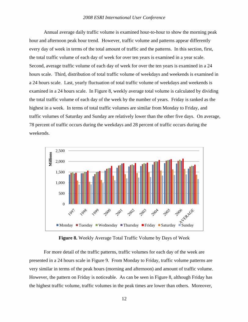
examined in a 24 hours scale. In Figure 8, weekly average total volume is calculated by dividing
the total traffic volume of each day of the week by the number of years. Friday is ranked as the
highest in a week. In terms of total traffic volumes are similar from Monday to Friday, and
traffic volumes of Saturday and Sunday are relatively lower than the other five days. On average,
78 percent of traffic occurs during the weekdays and 28 percent of traffic occurs during the
weekends.
Figure 8. Weekly Average Total Traffic Volume by Days of Week
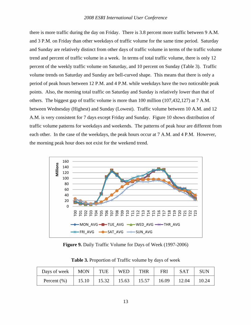
For more detail of the traffic patterns, traffic volumes for each day of the week are
presented in a 24 hours scale in Figure 9. From Monday to Friday, traffic volume patterns are
very similar in terms of the peak hours (morning and afternoon) and amount of traffic volume.
However, the pattern on Friday is noticeable. As can be seen in Figure 8, although Friday has
the highest traffic volume, traffic volumes in the peak times are lower than others. Moreover,
0
500
1,000
1,500
2,000
2,500
Mill
ions
Monday Tuesday Wednesday Thursday Friday Saturday Sunday
2008 ESRI International User Conference
13
there is more traffic during the day on Friday. There is 3.8 percent more traffic between 9 A.M.
and 3 P.M. on Friday than other weekdays of traffic volume for the same time period. Saturday
and Sunday are relatively distinct from other days of traffic volume in terms of the traffic volume
trend and percent of traffic volume in a week. In terms of total traffic volume, there is only 12
percent of the weekly traffic volume on Saturday, and 10 percent on Sunday (Table 3). Traffic
volume trends on Saturday and Sunday are bell-curved shape. This means that there is only a
period of peak hours between 12 P.M. and 4 P.M. while weekdays have the two noticeable peak
points. Also, the morning total traffic on Saturday and Sunday is relatively lower than that of
others. The biggest gap of traffic volume is more than 100 million (107,432,127) at 7 A.M.
between Wednesday (Highest) and Sunday (Lowest). Traffic volume between 10 A.M. and 12
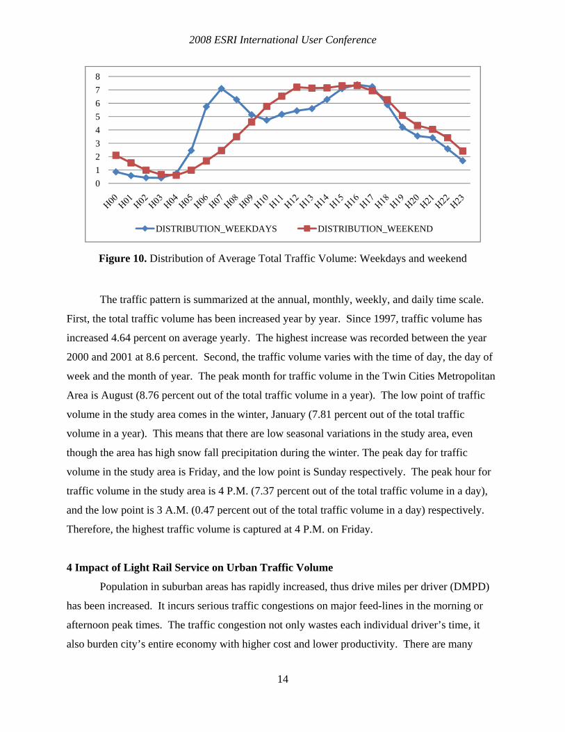
A.M. is very consistent for 7 days except Friday and Sunday. Figure 10 shows distribution of
traffic volume patterns for weekdays and weekends. The patterns of peak hour are different from
each other. In the case of the weekdays, the peak hours occur at 7 A.M. and 4 P.M. However,
the morning peak hour does not exist for the weekend trend.
Figure 9. Daily Traffic Volume for Days of Week (1997-2006)
Table 3. Proportion of Traffic volume by days of week
Days of week MON TUE WED THR FRI SAT SUN
Percent (%) 15.10 15.32 15.63 15.57 16.09 12.04 10.24
020406080
100120140160
T00
T01
T02
T03
T04
T05
T06
T07
T08
T09
T10
T11
T12
T13
T14
T15
T16
T17
T18
T19
T20
T21
T22
T23
Millions
MON_AVG TUE_AVG WED_AVG THR_AVG
FRI_AVG SAT_AVG SUN_AVG
2008 ESRI International User Conference
14
Figure 10. Distribution of Average Total Traffic Volume: Weekdays and weekend
The traffic pattern is summarized at the annual, monthly, weekly, and daily time scale.
First, the total traffic volume has been increased year by year. Since 1997, traffic volume has
increased 4.64 percent on average yearly. The highest increase was recorded between the year
2000 and 2001 at 8.6 percent. Second, the traffic volume varies with the time of day, the day of
week and the month of year. The peak month for traffic volume in the Twin Cities Metropolitan
Area is August (8.76 percent out of the total traffic volume in a year). The low point of traffic
volume in the study area comes in the winter, January (7.81 percent out of the total traffic
volume in a year). This means that there are low seasonal variations in the study area, even
though the area has high snow fall precipitation during the winter. The peak day for traffic
volume in the study area is Friday, and the low point is Sunday respectively. The peak hour for
traffic volume in the study area is 4 P.M. (7.37 percent out of the total traffic volume in a day),
and the low point is 3 A.M. (0.47 percent out of the total traffic volume in a day) respectively.
Therefore, the highest traffic volume is captured at 4 P.M. on Friday.
4 Impact of Light Rail Service on Urban Traffic Volume
Population in suburban areas has rapidly increased, thus drive miles per driver (DMPD)
has been increased. It incurs serious traffic congestions on major feed-lines in the morning or
afternoon peak times. The traffic congestion not only wastes each individual driver’s time, it
also burden city’s entire economy with higher cost and lower productivity. There are many
012345678
DISTRIBUTION_WEEKDAYS DISTRIBUTION_WEEKEND
2008 ESRI International User Conference
15
strategies to alleviate traffic volume on major highways such as developing public transit,
increasing the capacity of highways and controlling incoming traffic from major and minor
arterials. Among those strategies, light rail service provides transit service to people
continuously and regularly without traffic congestions.
The Metro bus system provides 198 bus routes in the entire metropolitan area, and
Hiawatha Light Rail Train (LRT) has provided one route between Minneapolis downtown and
the southern suburb of Bloomington, Minnesota since 2004. The Hiawatha Light Rail has
provided service since June, 2004 along the Highway 55 corridor. It provides services between
4:00 A.M. and 2:00 A.M. covering the 17 stations along 12 miles of service distance connecting
downtown Minneapolis, Minneapolis-St. Paul International Airport (MSP) and Mall of America
in Bloomington. In this case study, we investigate how the LRT affects the traffic system in the
Twin Cities metropolitan area based on traffic volume changes nearby the service area (Figure
11). The study area comprises with 19 links on major highways nearby the Hiawatha LRT
service area. In order to identify the impact, general traffic change pattern for 2000-2003 is
obtained using equation (1). Traffic change pattern in pre-event (June 24th, 2003-June 24th, 2004)
and post-event (June 25th, 2004-June 24th, 2005) is calculated using equation (2). The difference
is compared using equation (3).
∑ (1)
Where:
= {2003, 2002, 2001}
= Total traffic volume in year
(2)
Where:
= Total traffic volume in the post-service year
= Total traffic volume in the pre-service year
(3)
Where:
= Fluctuation of node N
= Average change of traffic volume
= Changes between the pre & post LRT service
2008 ESRI International User Conference
16
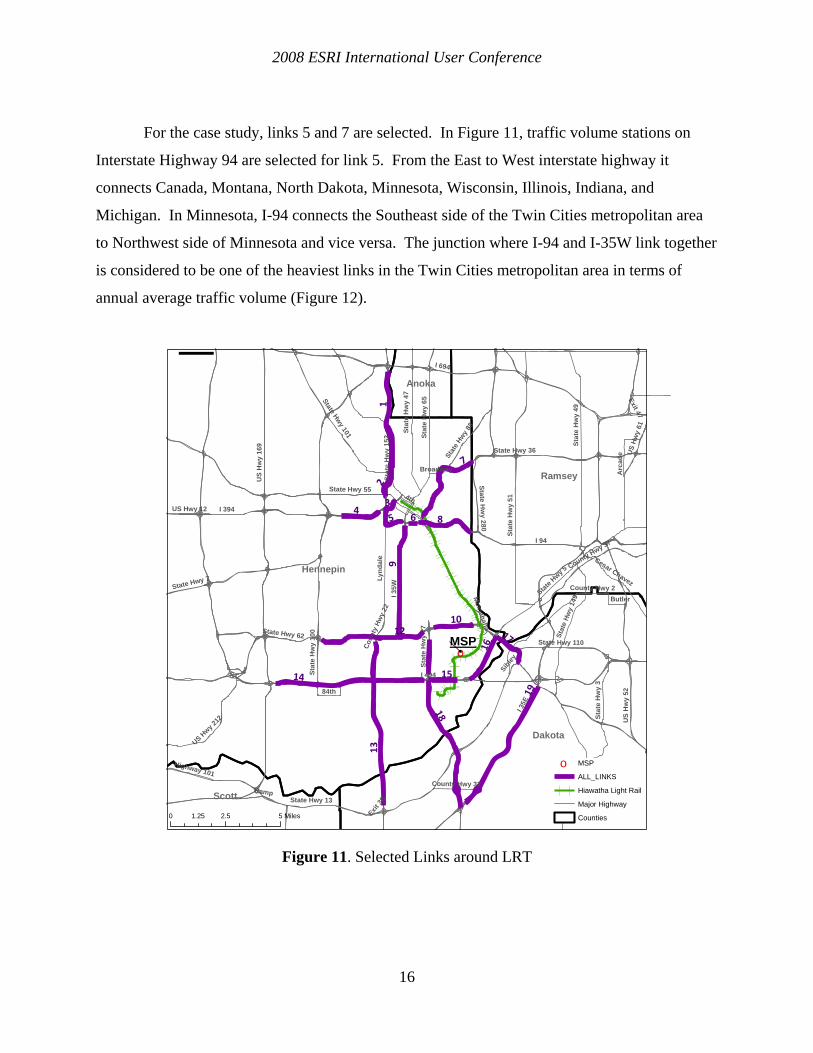
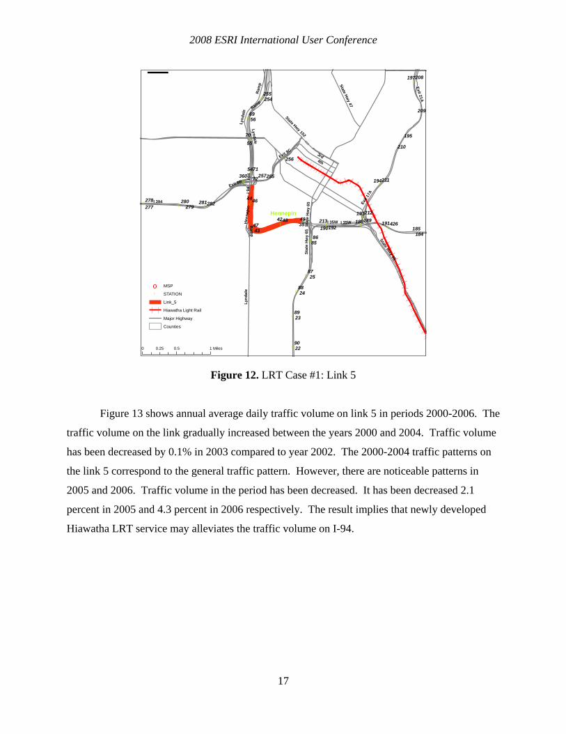
For the case study, links 5 and 7 are selected. In Figure 11, traffic volume stations on
Interstate Highway 94 are selected for link 5. From the East to West interstate highway it
connects Canada, Montana, North Dakota, Minnesota, Wisconsin, Illinois, Indiana, and
Michigan. In Minnesota, I-94 connects the Southeast side of the Twin Cities metropolitan area
to Northwest side of Minnesota and vice versa. The junction where I-94 and I-35W link together
is considered to be one of the heaviest links in the Twin Cities metropolitan area in terms of
annual average traffic volume (Figure 12).
Figure 11. Selected Links around LRT
o
Hennepin
Dakota
Ramsey
Scott
Anoka
I 494
I 35E
I 94
I 35W
I 694
US
Hw
y 16
9
I 394
Stat
e H
wy
100
US
Hw
y 52
State Hwy 55
State Hwy 13
Stat
e H
wy
77
Stat
e H
wy
51
Stat
e H
wy
3State Hwy 7
State Hwy 62
Stat
e H
wy
49
State Hwy 36
Lynd
ale
Highway 101
State H
wy 5
Stat
e H
wy
65
State Hwy 110
Stat
e Hw
y 14
9
US H
wy
61Stat
e H
wy
47
Stat
e Hwy 8
8
Stat
e H
wy
152
US Hwy 2
12
State Hwy 101
84th
State Hw
y 28 0
4thUS Hwy 12
Arc
ade
County Hwy 37
County Hwy 32Ramp
Sibley
County Hwy 2Butler
Broadway
Exit 3B
Minnehaha
Coun
ty H
wy
22
Cesar Chavez
Exit 47
19
14
7
1318
8
12
19
4
2
16
1017
5
15
63
MSP
¯
0 2.5 51.25 Miles
o MSP
ALL_LINKS
Hiawatha Light Rail
Major Highway
Counties
2008 ESRI International User Conference
17
Figure 12. LRT Case #1: Link 5
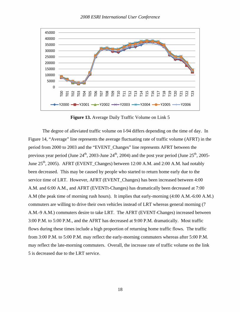
Figure 13 shows annual average daily traffic volume on link 5 in periods 2000-2006. The
traffic volume on the link gradually increased between the years 2000 and 2004. Traffic volume
has been decreased by 0.1% in 2003 compared to year 2002. The 2000-2004 traffic patterns on
the link 5 correspond to the general traffic pattern. However, there are noticeable patterns in
2005 and 2006. Traffic volume in the period has been decreased. It has been decreased 2.1
percent in 2005 and 4.3 percent in 2006 respectively. The result implies that newly developed
Hiawatha LRT service may alleviates the traffic volume on I-94.
!
!
!
!
!
!!
!!!
!!
!! !
!
!
!
!!
!
!
!
!
! !
!
!
!
!
!!! !!!
!!
!
!
!
!
!!
!
!
!
!
!
!!
!
!
!! !! !!
!! !
!
Hennepin
I 94
I 35W
I 394
State Hwy 55
Lynd
ale
4th
3rd
Stat
e H
wy
65
State Hwy 152R
amp State Hw
y 47
Hen
nepi
n
Exit 8B
Exit
17A
Exit 21A
Exit 9C
I 94
Lyndale
Lynd
ale
Sta t
e H
wy
65
Ramp
I 35WRam
p
90
89
88
87
8685
72
71
70
6956
55
54
494847
4644
43
4235
25
24
23
22
426
285
282281280279
278277
257
256
255254
213212
211
210
209
208197
195
194
193
192191
190189188
185184
360
¯
0 0.5 10.25 Miles
o MSP
! STATION
Link_5
Hiawatha Light Rail
Major Highway
Counties
2008 ESRI International User Conference
18
Figure 13. Average Daily Traffic Volume on Link 5
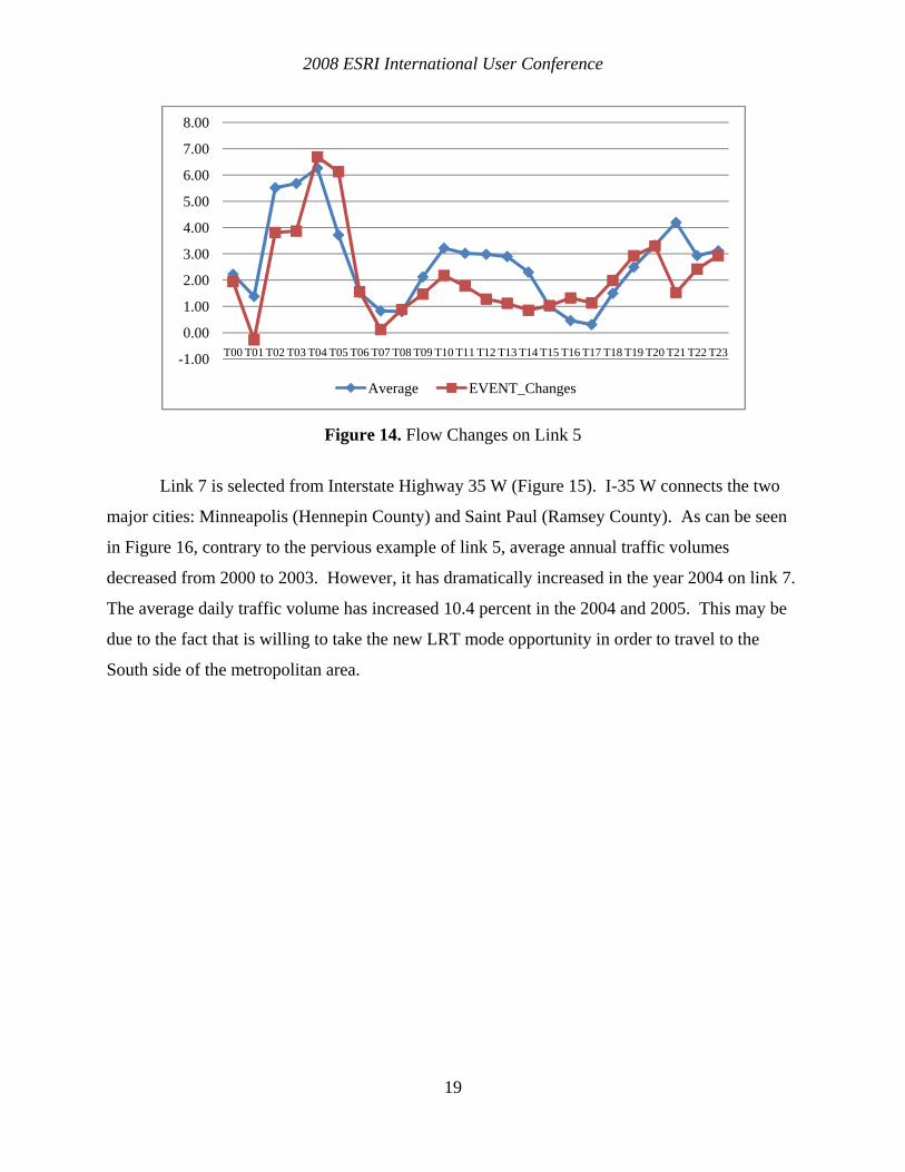
The degree of alleviated traffic volume on I-94 differs depending on the time of day. In
Figure 14, “Average” line represents the average fluctuating rate of traffic volume (AFRT) in the
period from 2000 to 2003 and the “EVENT_Changes” line represents AFRT between the
previous year period (June 24th, 2003-June 24th, 2004) and the post year period (June 25th, 2005-
June 25th, 2005). AFRT (EVENT_Changes) between 12:00 A.M. and 2:00 A.M. had notably
been decreased. This may be caused by people who started to return home early due to the
service time of LRT. However, AFRT (EVENT_Changes) has been increased between 4:00
A.M. and 6:00 A.M., and AFRT (EVENTt-Changes) has dramatically been decreased at 7:00
A.M (the peak time of morning rush hours). It implies that early-morning (4:00 A.M.-6:00 A.M.)
commuters are willing to drive their own vehicles instead of LRT whereas general morning (7
A.M.-9 A.M.) commuters desire to take LRT. The AFRT (EVENT-Changes) increased between
3:00 P.M. to 5:00 P.M., and the AFRT has decreased at 9:00 P.M. dramatically. Most traffic
flows during these times include a high proportion of returning home traffic flows. The traffic
from 3:00 P.M. to 5:00 P.M. may reflect the early-morning commuters whereas after 5:00 P.M.
may reflect the late-morning commuters. Overall, the increase rate of traffic volume on the link
5 is decreased due to the LRT service.
0
5000
10000
15000
20000
25000
30000
35000
40000
45000
T00
T01
T02
T03
T04
T05
T06
T07
T08
T09
T10
T11
T12
T13
T14
T15
T16
T17
T18
T19
T20
T21
T22
T23
Y2000 Y2001 Y2002 Y2003 Y2004 Y2005 Y2006
2008 ESRI International User Conference
19
Figure 14. Flow Changes on Link 5
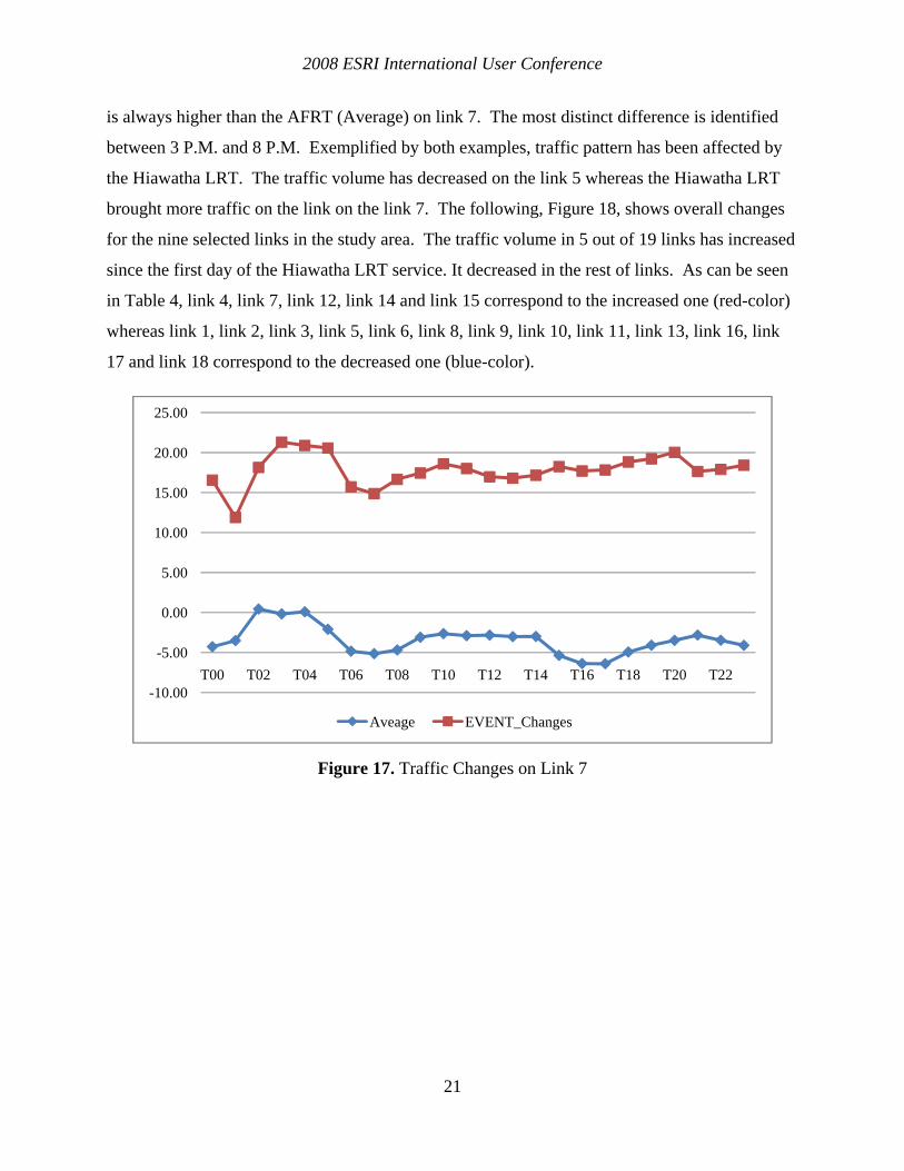
Link 7 is selected from Interstate Highway 35 W (Figure 15). I-35 W connects the two
major cities: Minneapolis (Hennepin County) and Saint Paul (Ramsey County). As can be seen
in Figure 16, contrary to the pervious example of link 5, average annual traffic volumes
decreased from 2000 to 2003. However, it has dramatically increased in the year 2004 on link 7.
The average daily traffic volume has increased 10.4 percent in the 2004 and 2005. This may be
due to the fact that is willing to take the new LRT mode opportunity in order to travel to the
South side of the metropolitan area.
-1.00
0.00
1.00
2.00
3.00
4.00
5.00
6.00
7.00
8.00
T00 T01 T02 T03 T04 T05 T06 T07 T08 T09 T10 T11 T12 T13 T14 T15 T16 T17 T18 T19 T20 T21 T22 T23
Average EVENT_Changes
2008 ESRI International User Conference
20
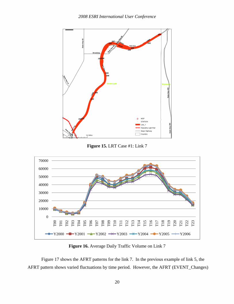
Figure 15. LRT Case #1: Link 7
Figure 16. Average Daily Traffic Volume on Link 7
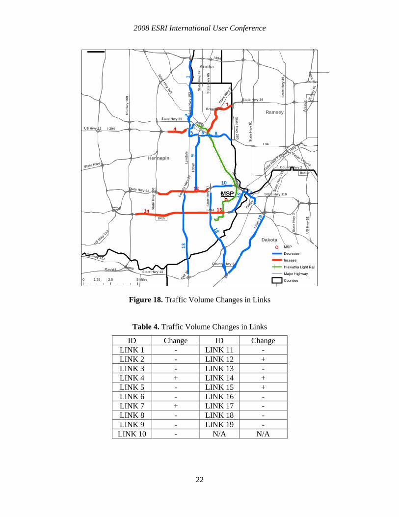
Figure 17 shows the AFRT patterns for the link 7. In the previous example of link 5, the
AFRT pattern shows varied fluctuations by time period. However, the AFRT (EVENT_Changes)
!
!
!
!
!
!
!
!
!
!
!
!
!
!
Hennepin Ramsey
I 35W
Stat
e H
wy
280
Stat
e H
wy
65
Broadway
Stat
e Hwy 8
8
Ramp Exit 21A
State Hwy 47
State Hwy 55
Exit
17A
Ramp
Stat
e H
wy
280
I 35W
State H
wy 88
Exit 21A
211
210
209
208
207
206
205
200
199
198
197
196
195
194
¯
0 0.3 0.60.15 Miles
o MSP
! STATION
Link_7
Hiawatha Light Rail
Major Highway
Counties
0
10000
20000
30000
40000
50000
60000
70000
T00
T01
T02
T03
T04
T05
T06
T07
T08
T09
T10
T11
T12
T13
T14
T15
T16
T17
T18
T19
T20
T21
T22
T23
Y2000 Y2001 Y2002 Y2003 Y2004 Y2005 Y2006
2008 ESRI International User Conference
21
is always higher than the AFRT (Average) on link 7. The most distinct difference is identified
between 3 P.M. and 8 P.M. Exemplified by both examples, traffic pattern has been affected by
the Hiawatha LRT. The traffic volume has decreased on the link 5 whereas the Hiawatha LRT
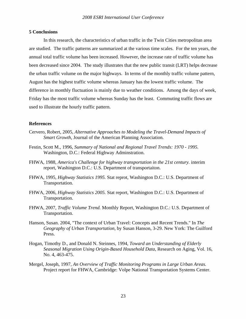
brought more traffic on the link on the link 7. The following, Figure 18, shows overall changes
for the nine selected links in the study area. The traffic volume in 5 out of 19 links has increased
since the first day of the Hiawatha LRT service. It decreased in the rest of links. As can be seen
in Table 4, link 4, link 7, link 12, link 14 and link 15 correspond to the increased one (red-color)
whereas link 1, link 2, link 3, link 5, link 6, link 8, link 9, link 10, link 11, link 13, link 16, link
17 and link 18 correspond to the decreased one (blue-color).
Figure 17. Traffic Changes on Link 7
-10.00
-5.00
0.00
5.00
10.00
15.00
20.00
25.00
T00 T02 T04 T06 T08 T10 T12 T14 T16 T18 T20 T22
Aveage EVENT_Changes
2008 ESRI International User Conference
22
Figure 18. Traffic Volume Changes in Links
Table 4. Traffic Volume Changes in Links
ID Change ID Change LINK 1 - LINK 11 - LINK 2 - LINK 12 + LINK 3 - LINK 13 - LINK 4 + LINK 14 + LINK 5 - LINK 15 + LINK 6 - LINK 16 - LINK 7 + LINK 17 - LINK 8 - LINK 18 - LINK 9 - LINK 19 - LINK 10 - N/A N/A
o
Hennepin
Dakota
Ramsey
Scott
Anoka
I 494
I 35E
I 94
I 35W
I 694
US
Hw
y 16
9I 394
Stat
e H
wy
1 00
US
Hw
y 52
State Hwy 55
State Hwy 13
Stat
e H
wy
77
Stat
e H
wy
51
Stat
e H
wy
3
State Hwy 7
State Hwy 62
Stat
e H
wy
49
State Hwy 36
Lynd
a le
Highway 101
State H
wy 5
Stat
e H
wy
65
State Hwy 110
Stat
e Hw
y 14
9
US H
wy
61Stat
e H
wy
47
Stat
e Hwy 8
8
Stat
e H
wy
152
US Hwy 2
12
State Hwy 101
84th
State Hw
y 28 0
4thUS Hwy 12
Arc
ade
County Hwy 37
County Hwy 32Ramp
Sibley
County Hwy 2Butler
Broadway
Exit 3B
Minnehaha
Coun
ty H
wy
22
Cesar Chavez
Exit 47
14
7
12
4
15
19
1318
8
19
2
16
1017
5 63
MSP
¯
0 2.5 51.25 Miles
o MSP
Decrease
Incease
Hiawatha Light Rail
Major Highway
Counties
2008 ESRI International User Conference
23
5 Conclusions
In this research, the characteristics of urban traffic in the Twin Cities metropolitan area
are studied. The traffic patterns are summarized at the various time scales. For the ten years, the
annual total traffic volume has been increased. However, the increase rate of traffic volume has
been decreased since 2004. The study illustrates that the new public transit (LRT) helps decrease
the urban traffic volume on the major highways. In terms of the monthly traffic volume pattern,
August has the highest traffic volume whereas January has the lowest traffic volume. The
difference in monthly fluctuation is mainly due to weather conditions. Among the days of week,
Friday has the most traffic volume whereas Sunday has the least. Commuting traffic flows are
used to illustrate the hourly traffic pattern.
References
Cervero, Robert, 2005, Alternative Approaches to Modeling the Travel-Demand Impacts of Smart Growth, Journal of the American Planning Association.
Festin, Scott M., 1996, Summary of National and Regional Travel Trends: 1970 - 1995. Washington, D.C.: Federal Highway Adminstration.
FHWA, 1988, America's Challenge for highway transportation in the 21st century. interim report, Washington D.C.: U.S. Department of transportaiton.
FHWA, 1995, Highway Statistics 1995. Stat reprot, Washington D.C.: U.S. Department of Transportation.
FHWA, 2006, Highway Statistics 2005. Stat report, Washington D.C.: U.S. Department of Transportation.
FHWA, 2007, Traffic Volume Trend. Monthly Report, Washington D.C.: U.S. Department of Transportation.
Hanson, Susan. 2004, "The context of Urban Travel: Concepts and Recent Trends." In The Geography of Urban Transportation, by Susan Hanson, 3-29. New York: The Guilford Press.
Hogan, Timothy D., and Donald N. Steinnes, 1994, Toward an Understanding of Elderly Seasonal Migration Using Origin-Based Household Data, Research on Aging, Vol. 16, No. 4, 463-475.
Mergel, Joseph, 1997, An Overview of Traffic Monitoring Programs in Large Urban Areas. Project report for FHWA, Cambridge: Volpe National Transportation Systems Center.
2008 ESRI International User Conference
24
MPX, 2007, "NOAA's National Weather Service." NOAA's National Weather Service Weather Forecast Office. 1 20, 2006. http://www.crh.noaa.gov/mpx/mspSnowfall.php (accessed 11 14, 2007).
Nancy, McGuckin, and Nanda, Srinivasan, 2003, Journey to Work Trends in the United States and its Major Metropolitan Areas 1960 - 2000. Government Accession, Washington D.C.: US Department of Transportation.
Schrank, D. and T. Lomax, 2004, Urban Mobility Report. Houston: Texas Transportation Institute.
Tully, Shawn, 2007, "The 500 largest U.S. corporations." Fortune.
US Census Bureau, 2000, Retrieved December 2007 from www.census.gov.