Spatial Capture-Recapture Models for JointlyEstimating Population Density and Landscape

Connectivity

J. Andrew Royle, Richard B. Chandler, Kimberly D. GazenskiUSGS Patuxent Wildlife Research Center, Laurel MD

Tabitha A. Graves∗

Northern Arizona University, Flagstaff AZ

October 18, 2012

Abstract Population density and landscape connectivity are key determinants of1

population viability, yet no methods exist for simultaneously estimating density and2

connectivity parameters. Recently-developed spatial capture-recapture (SCR) models3

provide a framework for estimating density of animal populations, but thus far have not4

been used to study connectivity. Rather, all applications of SCR models have used5

encounter probability models based on the Euclidean distance between traps and animal6

activity centers, which implies that home ranges are stationary and symmetric, and7

unaffected by landscape structure. In this paper we devise encounter probability models8

based on “ecological distance”, i.e., the least-cost path between traps and activity centers,9

which is a function of both Euclidean distance and animal movement behavior in resistant10

landscapes. We integrate least-cost path models into a likelihood-based estimation scheme11

∗Current Address: Colorado State University, Warner College of Natural Resources, 201 JVK Wagar.Fort Collins, CO 80523

1

for spatial capture-recapture models in order to estimate population density and12

parameters of the least-cost encounter probability model. Therefore, it is possible to make13

explicit inferences about animal density, distribution, and landscape connectivity as it14

relates to animal movement from standard capture-recapture data. Furthermore, a15

simulation study demonstrated that ignoring landscape connectivity can result in16

negatively biased density estimators under the naive SCR model.17

Key words: animal movement, ecological distance, landscape connectivity, least-cost18

path, resistance surface, spatial capture-recapture19

1 Introduction20

Assessing the impacts of habitat fragmentation and habitat loss on population density and21

landscape connectivity are high priorities in applied ecological research. Landscape connec-22

tivity is defined as the degree to which landscape structure impedes or facilitates movement23

(Tischendorf and Fahrig, 2000) and is widely recognized to be an important component of24

population viability (With and Crist, 1995). Although much theory has been developed to25

predict the effects of decreasing connectivity, few empirical studies have been conducted to26

test these predictions due to the paucity of formal methods for estimating connectivity pa-27

rameters (Cushman et al., 2010). Instead, ecologists often rely on expert opinion or ad hoc28

methods of specifying connectivity values, even in important applied settings (Adriaensen29

et al., 2003; Beier et al., 2008; Zeller et al., 2012). In addition, no methods are available for30

simultaneously estimating population density and connectivity parameters, in spite of theory31

predicting interacting effects of density and connectivity on population viability (Tischendorf32

et al., 2005; Cushman et al., 2010).33

Spatial capture-recapture (SCR) models are a relatively new class of models allowing for34

2

inference about both population density and movement (Efford, 2004; Borchers and Efford,35

2008; Royle and Young, 2008; Efford et al., 2009; Royle et al., 2009). While SCR models are36

a relatively recent innovation, their use is already becoming widespread (Efford et al., 2009;37

Gardner et al., 2010b,a; Kery et al., 2010; Gopalaswamy et al., 2012; Foster and Harmsen,38

2012) because they resolve critical problems with ordinary non-spatial capture-recapture39

methods such as ill-defined area sampled and heterogeneity in encounter probability due40

to the juxtaposition of individuals with traps. Furthermore, all capture-recapture studies41

produce auxiliary spatial information and therefore SCR models are widely applicable.42

In spite of their utility for estimating population density, SCR methods are still in their43

infancy, and so far, every application has implicitly assumed that animals have isotropic44

home ranges and that movement is unaffected by landscape structure. Specifically, existing45

SCR models assume that encounter probability is a simple function of the Euclidean distance46

between an individual’s activity center (e.g. its home range or territory center) and the trap47

location. While these simple encounter probability models will often be sufficient for some48

purposes, especially in small data sets, animals may not judge distance in terms of Euclidean49

distance but, rather, according to the quality of local habitat, perceived mortality risk, and50

other considerations that facilitate or impede movement. Because encounter probability and51

the distance metric upon which it is based represent outcomes of individual movements about52

their home range, it is desirable to relax the Euclidean distance assumption of SCR models53

such that hypotheses about landscape connectivity can be evaluated.54

In this paper we develop models for encounter probability based on alternative distance55

metrics that account for connectivity—which, in keeping with the conventions in the eco-56

logical literature, we will call “ecological distance”. In particular, we adopt a cost-weighted57

distance metric to define the least-cost path, which is used widely in landscape ecology for58

3

modeling resistance to movement and gene flow (Adriaensen et al., 2003). In the context of59

SCR models we can use this as the basis for defining the distance between traps and individ-60

ual’s activity centers. In this way we can explicitly model the effects of landscape structure61

on movement. We develop a likelihood-based inference framework that allows estimation of62

the parameters of the cost function so that direct inference about density and connectivity63

can be made from capture-recapture data without subjective prescription of resistance or64

cost surfaces.65

2 Spatial Capture-Recapture66

The basic idea of SCR is to express encounter probability as a function of the distance be-67

tween an individual’s activity center, say s, and a trap location, say x (Borchers and Efford,68

2008). The definition of an activity will be context-specific, but often it will be the center69

of an individual’s home range, or more generally, the spatial average of an individual’s loca-70

tions during some time period. SCR methods regard the activity centers as latent variables71

following some spatial point process, such as the homogeneous model s ∼ Uniform(S) where72

S is a spatial region (the “state-space” of s) (Royle and Young, 2008). The state-space S73

defines the potential locations for any activity center s, e.g., a polygon defining available74

habitat or range of the species under study.75

A number of distinct encounter models have been proposed for spatial capture-recapture76

situations (Borchers and Efford, 2008; Royle et al., 2009; Efford et al., 2009), including77

Poisson, multinomial or binomial models. Here we focus on the binomial model in which we78

suppose that J traps at locations xj are operated for K occasions (e.g., nights), although our79

development of ecological distance models is directly applicable to other observation models80

without any further technical considerations. The binomial model is most directly relevant81

4

to devices such as hair snares (Woods et al., 1999; Gardner et al., 2010b) or scent sticks82

(Kery et al., 2010) for which individuals can only be encountered at most once in a trap per83

observation occasion.84

The observations are individual- and trap-specific counts yij which are binomial with85

sample size K and probabilities pij. The vector of trap-specific counts for individual i,86

yi = (yi1, . . . , yiJ) is its encounter history. A standard encounter probability model (Borchers87

and Efford, 2008) is the Gaussian model in which88

log(pij) = α0 + α1d(xj, si)2 (1)

or, equivalently, pij = λ0exp(−d(xj, si)2/(2σ2)) where α0 = log(λ0) and α1 = −1/(2σ2) and89

d(xj, si) is the Euclidean distance between trap j and activity center i.90

Although alternative detection models are often used, all are functions of Euclidean dis-91

tance and so we do not consider them further. The distance metric we develop subsequently92

can be used in conjunction with any other detection model. In all previous applications93

of SCR models the Euclidean distance has been used, i.e., d(xj, si) = ||xj − si||, and the94

parameters α0 and α1 have been estimated using standard methods (likelihood or Bayesian).95

The critical assumption that motivates our work is that the Euclidean distance metric is96

unaffected by habitat or landscape structure, and it implies that the space used by individuals97

is stationary (invariant to translation) and symmetric which may be unreasonable in some98

applications. For example, if the common detection model based on a bivariate normal99

probability distribution function is used, then the implied space usage by all individuals, no100

matter their location in space or local habitat conditions, is symmetric with circular contours101

of usage intensity (density contours of the probability density). Subsequently we provide an102

extension of this class of SCR models that accommodates alternative distance metrics that103

5

explicitly incorporate information about the landscape so that a unit of distance is variable104

depending on identified covariates. Thus, where an individual lives on the landscape, and105

the state of the surrounding landscape, will determine the nature of its usage of space. In106

particular, we suggest distance metrics that imply irregular, asymmetric and non-stationary107

home ranges of individuals. An example of this is shown in Fig. 1 which shows home ranges108

of 4 individuals for a specific landscape, described below.109

3 Cost-Weighted Distance110

We adopt the use of a cost-weighted distance metric here which defines the distance between111

locations by accumulating cell-specific costs determined under a cost function defined by the112

user. The idea of cost-weighted distance to characterize animal use of landscapes is widely113

used in landscape ecology for modeling connectivity, movement and gene flow (Beier et al.,114

2008). As is customary for reasons of computational tractability we consider a discrete115

landscape defined by cells of some prescribed resolution. The distance between any two116

locations x and x′ can be represented by a sequence of line segments connecting neighboring117

cells say l1, l2, . . . , lm. Then the total cost-weighted distance between x and x′ is118

d(x,x′) =m−1∑i=1

cost(li, li+1)||li − li+1|| (2)

where cost(li, li+1) is the user-defined cost function to move from cell li to neighboring cell119

li+1 in the sequence. Given the “cost” of each cell, it is a simple matter to compute the cost-120

weighted distance between any two cells, along any path, by accumulating the incremental121

cost-weighted distances. In the context of SCR models (and, more generally, landscape122

connectivity) we are concerned with the minimum cost-weighted distance, that of the least-123

6

cost path, between any two locations which we will denote by dlcp, which is the sequence124

l1, l2, . . . , lm that minimizes Eq. 2. That is,125

dlcp(x,x′) = minl1,...,lm

m−1∑i=1

cost(li, li+1)||li − li+1|| (3)

Least-cost path can be calculated in many geographic information systems and other software126

packages, including the R package gdistance (van Etten, 2011).127

The key ecological aspect of least-cost path modeling is the development of models for128

cell-specific cost (also called resistance in the landscape ecology literature). In this paper we129

model cost as a log-linear function of covariates defined on every cell, i.e., z(x) is the value130

of some covariate at location x. Then, we model cost of moving from a cell x to one of its131

neighbors, say x′, by the weighted average132

log(cost(x,x′)) = α2z(x) + z(x′)

2(4)

where α2 is the resistance parameter to be estimated. Thus, if α2 = 0 then substituting133

cost(x,x′) = exp(0) = 1 into Eq. 3 will produce the ordinary Euclidean distance between134

points.135

In practical applications, variables that influence the cost of moving across the landscape136

include highways (e.g., Epps et al., 2005), elevation (Cushman et al., 2006), snow cover137

(Schwartz et al., 2009), distance to escape terrain (Shirk et al., 2010), or range limitations138

(McRae and Beier, 2007). Together multiple environmental variables create a resistance sur-139

face, which forms the linchpin of all connectivity planning (Spear et al., 2010). Although α2140

is never known in practice, conservation biologists design linkages that require this resistance141

value as input (see Beier et al., 2008, and articles cited therein). Therefore, investigators142

often choose a value for α2 based on expert opinion (Beier et al., 2008), although recently143

7

researchers have begun to define costs based on resource selection functions, animal move-144

ment (Tracy, 2006; Fortin et al., 2005), or genetic distance data (Gerlach and Musolf, 2000;145

Schwartz et al., 2009). Our paper represents the first formal approach to estimating land-146

scape resistance parameters from capture-recapture data.147

To formalize the use of cost-weighted distance in SCR models, we substitute Eq. 3 in148

the expression for encounter probability (Eq. 1) and maximize the resulting likelihood (see149

Maximum Likelihood Estimation), including for estimating the parameter α2. An example150

of computing cost-weighted distance in R for a simple landscape is given in Appendix 1.151

3.1 Non-stationarity of home range structure152

When distance is defined by the cost-weighted distance metric given by Eq. 3 then individual153

space-usage varies spatially in response to the landscape covariate(s) used in the distance154

metric. For example, we use the two landscapes shown in Fig. 2 in our simulation study155

below. The landscape shown in the right panel, with distance metric defined by Eq. 3,156

produces home ranges such as those shown in Fig. 1. Later we simulate data under the157

model that produces these home ranges and fit spatial capture-recapture models to evaluate158

the efficacy of likelihood estimation under this model.159

4 Maximum likelihood estimation160

Here we outline a standard method of parameter estimation based on marginal likelihood.161

That is, the likelihood in which the latent variables s are removed by integration (Borchers162

and Efford, 2008). The individual- and trap-specific observations have a binomial distribution163

conditional on the latent variable si:164

8

yij|si ∼ Binomial(K, pα(dlcp(xj, si;α2);α0, α1) (5)

where we have indicated the dependence of p on the parameters α = (α0, α1, α2), and also165

dlcp which itself depends on α2, and the latent variable s. For the random effect we have si ∼166

Uniform(S). The joint distribution of the data for individual i is the product of J binomial167

terms (i.e., contributions from each of J traps): [yi|si,α] =∏J

j=1 Binomial(K, pα(xj, si)).168

The so-called marginal likelihood is computed by removing si, by integration, from the169

conditional-on-s likelihood and regarding the marginal distribution of the data as the likeli-170

hood. That is, we compute:171

[yi|α] =

∫S[yi|si,α]g(si)dsi

where, under the uniformity assumption, we have g(s) = 1/||S||. The joint likelihood for all172

N individuals, is the product of N such terms:173

L(α|y1,y2, . . . ,yN) =N∏i=1

[yi|α]

Because N is unknown, we have to accommodate the contribution of N − n “all-zero”174

encounter histories (i.e., yij = 0 for all j). We include the number of such all-zero encounter175

histories as an unknown parameter of the model, which we label n0. In addition, we have to be176

sure to include a combinatorial term to account for the fact that of the n observed individuals177

there are(Nn

)ways to realize a sample of size n. The combinatorial term involves the178

unknown n0 and thus it must be included in the likelihood. Technical details for computing179

the likelihood and obtaining the MLEs are given in Appendix 2 where we provide an R180

function to evaluate the likelihood and obtain the MLEs. A key practical detail is that181

9

the likelihood here is formulated in terms of the parameter N , the population size for the182

landscape defined by S. Given S, density is computed as D(S) = N/||S|| where ‖S‖ is the183

area of the state space. In our simulation study below we report N as the two are equivalent184

summaries of the data set once S is defined.185

5 Examples186

In this section we provide examples that we think are typical of how cost-weighted distance187

models can be used in real capture-recapture problems. We define a 20× 20 cell landscape188

with extent = [0.5, 4.5] × [0.5, 4.5]. We suppose that 16 camera traps are established at189

the integer coordinates (1, 1), (1, 2), . . . , (4, 4). We could think of this as a landscape within190

which we’re studying a population of ocelots, lynx or some other species using camera traps.191

For our analyses, cost is characterized by a single covariate and we consider two specific192

cases. First is an increasing trend from the NW to the SE (“systematic landscape”), where193

z(x) is defined as z(x) = r(x) + c(x) where r(x) and c(x) are just the row and column,194

respectively, of the landscape. This might define something related to distance from an195

urban area or a gradient in habitat quality due to land use, or environmental conditions196

such as temperature or precipitation gradients. In the second case we make up a covariate197

by generating a field of spatially correlated noise to emulate fragmented habitat. The two198

covariates are shown in Fig. 2, along with a sample realization of N = 100 individuals (left199

panel only). For both covariates we use a cost function in which transitions from cell x to200

x′ is given by:201

log(cost(x,x′)) = α2z(x) + z(x′)

2

10

where α2 = 1 for our simulation.202

5.1 Simulation study203

We devised a limited simulation study to evaluate three things: (1) the general statistical204

performance of the density estimator under this new model; (2) the effect of mis-specifying205

the model with a normal Euclidean distance metric and (3) the statistical performance of206

estimating the resistance parameter, α2.207

We used population sizes of 100 and 200 individuals with activity centers randomly208

distributed on the 20× 20 landscape, and subjected them to encounter by 16 traps arranged209

in a 4 × 4 grid according to the Euclidean distance metric. We fit 3 different models; (i)210

the misspecified Euclidean distance model; (ii) the true data-generating model with the cost211

known and (iii) the true data-generating model but estimating the resistance parameter212

by maximum likelihood. We used the “systematic” and “fragmented” covariates defined213

previously.214

We simulated encounter data for the N individuals using the Gaussian encounter model215

with least-cost path distance metric:216

log(pij) = α0 + α1dlcp(xj, si;α2)2

We used here α0 = −2 and α1 = 2, the latter value corresponding to σ = 0.5 of a stationary217

bivariate normal home range model. We varied the number of replicate samples K = 3, 5, 10218

(e.g., nights in a camera trapping study) to produce varying sample sizes. Because any sim-219

ulation study is inherently arbitrary, we have provided R scripts for carrying out simulations220

in Appendix 2 so that the interested reader can experiment with their own situations.221

11

5.2 Simulation Results222

For both landscapes and all simulation conditions (levels of K and N) the average sample223

sizes of individuals captured are given in Appendix 4. The simulation results for estimating224

N for the prescribed state-space are given in Table 1. For the fragmented landscape we225

see extreme bias in estimates of N when the Euclidean distance is used. There is moderate226

small sample bias of 3-5% in the MLE of N using the least-cost path distance which becomes227

negligible asK increases. ForN = 200 the bias is on the order of 2% for the lowest sample size228

case (K = 3) but negligible otherwise. Interestingly, for the landscape exhibiting systematic229

trend, there is a persistent bias in the MLE of N of 1-3% even for the highest level of K.230

We were initially surprised by this but, in fact, it results from the state-space being small231

relative to the extent of the trap grid, and sensitivity to a state-space that is too small is232

expected because the support of the integrand is truncated. In the particular case of the233

systematic landscape, we find that, on some edges of the landscape where cost of movement234

is low, individuals use large areas of space, and the fitted model is under-stating the apparent235

heterogeneity in encounter probability for the prescribed landscape. We found that the issue236

is resolved when the traps are moved away from the boundary (see Appendix 4).237

The performance of estimating the resistance parameter α2 mirrors the results for esti-238

mating N for the prescribed area (Appendix 4). In the fragmented landscape where we don’t239

expect a systematic gradient in space usage around the edge of the state-space, we find that240

α2 is estimated with diminishing bias as the sample size increases, but with persistent bias241

due to truncation of the likelihood for the systematic landscape which, as with the MLE242

of N , is resolved by moving the traps away from the edge of the prescribed landscape S.243

Equivalently, in practice, this could be resolved by expanding S away from the trap locations244

so that all regions used by animals exposed to capture are included in S.245

12

6 Discussion246

Inferences about population density and landscape connectivity are fundamental to many247

problems in applied and theoretical ecology such as the assessment of fragmentation effects,248

corridor and reserve design, gene flow, and population viability analysis. Our model allows249

investigators to address these problems using non-invasively collected capture-recapture data250

by evaluating the landscape factors influencing movement. Our approach involves replacing251

the ordinary Euclidean distance metric in SCR models with an “ecological distance” metric252

defined as the minimum cost-weighted distance (i.e., “least-cost path”) between points, and253

where “cost” is characterized by one or more spatially explicit covariates that are believed254

to influence movement. Unlike many previous efforts, we presented methods for estimating255

the parameters of the cost function, thereby eliminating the need to subjectively prescribe256

their value.257

Animal movement is associated with various behaviors such as dispersal and migration,258

which may operate over many spatial and temporal scales. For simplicity, we considered259

movement around fixed home range centers, and thus our model is most applicable to short260

time intervals such as a single breeding season. Connectivity at this time scale is important261

because, for example, it can determine which breeding individuals interact. When interest262

lies in the effects of connectivity on more complex movement behaviors such as dispersal,263

we expect that it would be possible to extend our model to allow for movement of the264

activity centers themselves. Specifically, we envision cost-weighted distance functions that265

would describe the location of activity centers at time t as a function of their location at266

time t − 1 and the landscape structure surrounding the initial location (Gardner et al.,267

2010a). By adopting this type of open population model, it might also be possible to study268

the factors affecting dispersal propensity and survival during dispersal. Several capture-269

13

recapture methods exist for modeling dispersal (Kendall and Nichols, 2004; Fujiwara et al.,270

2006; Ovaskainen et al., 2008), but none allows for estimation of density and landscape271

connectivity.272

Our paper also has implications for existing SCR studies. Not surprisingly, our simulation273

study demonstrated (Tab. 1) that the MLE of model parameters is approximately unbiased274

in moderate sample sizes. Moreover, the effect of ignoring ecological distance and using275

normal Euclidean distance in the model for encounter probability, has the logical effect of276

causing negative bias in estimates of N . We expect this because the effect is similar to277

failing to model heterogeneity, i.e., if we mis-specify “model Mh” with “model M0” (Otis278

et al., 1978) then we will expect to under-estimate N (Royle and Dorazio, 2008, p. 193).279

So the effect of mis-specifying the ecological distance metric with a standard homogeneous280

Euclidean distance has the same effect. As a practical matter, it stands to reason that281

many previous applications of SCR models based on homogeneous distance metrics have282

under-stated density of the focal population.283

Our approach to modeling landscape connectivity does not include an explicit model284

of animal movement. That is, we cannot make inferences about the precise location of285

movement paths taken between recapture events or temporal decisions made by the animal286

as it moves about the landscape. Rather, our model describes the probability that an287

animal is captured at a trap based on the landscape context associated with the trap and288

the animal’s activity center. Equivalently, our model describes the process by which animals289

use space, and thus could be regarded as a model of resource selection. Although this is290

more phenomenological than an explicit movement model, it is consistent with the concepts291

of landscape connectivity and resistance. Furthermore, it is possible that our model could292

be expanded to accommodate telemetry data or other information if movement behavior is293

14

of interest.294

Some additional methodological extensions may be of general interest. We adopted a295

standard approach to inference under our model based on marginal likelihood but, in prin-296

ciple, Bayesian analysis does not pose any unique challenges for this class of models, except297

that computing the cost-weighted distance is computationally intensive and having to do this298

at each iteration of an MCMC algorithm may be impractical. We have used least-cost paths299

here to represent ecological distance although other distance metrics could be used, includ-300

ing circuit resistance distances (McRae, 2006). Instead of characterizing cost with explicit301

covariates it might be possible to estimate the “resistance surface” as a latent field, much as302

Wikle (2003) did in the developing of models of species spread based on a diffusion process.303

He defined the spatially-explicit rate of diffusion, δ(x), as a Gaussian spatial process, and it304

was estimated from the data.305

Capture-recapture methods are one of the most common technique for studying animal306

populations and, with new technologies such as camera trapping and DNA sampling, it is307

possible to conduct research on species that previously could not be studied. Our mod-308

eling framework makes it feasible to use basic capture-recapture data to study landscape309

connectivity and density simultaneously.310

15

References311

Adriaensen, F., J. P. Chardon, G. De Blust, E. Swinnen, S. Villalba, H. Gulinck, and312

E. Matthysen, 2003. The application of ‘least-cost’ modelling as a functional landscape313

model. Landscape and urban planning 64:233–247.314

Beier, P., D. R. Majka, and W. D. Spencer, 2008. Forks in the road: choices in procedures315

for designing wildland linkages. Conservation Biology 22:836–851.316

Borchers, D. L. and M. G. Efford, 2008. Spatially explicit maximum likelihood methods for317

capture–recapture studies. Biometrics 64:377–385.318

Cushman, S. A., B. W. Compton, and K. McGarigal, 2010. Habitat fragmentation effects319

depend on complex interactions between population size and dispersal ability: Modeling320

influences of roads, agriculture and residential development across a range of life-history321

characteristics. In S. A. Cushman and F. Huettmann, editors, Spatial complexity, infor-322

matics, and wildlife conservation, chapter 20, pages 369–385. Springer, New York.323

Cushman, S. A., K. S. McKelvey, J. Hayden, and M. K. Schwartz, 2006. Gene flow in324

complex landscapes: testing multiple hypotheses with causal modeling. The American325

Naturalist 168:486–499.326

Efford, M., 2004. Density estimation in live-trapping studies. Oikos 106:598–610.327

Efford, M. G., D. K. Dawson, and D. L. Borchers, 2009. Population density estimated from328

locations of individuals on a passive detector array. Ecology 90:2676–2682.329

Epps, C. W., P. J. Palsbøll, J. D. Wehausen, G. K. Roderick, R. R. Ramey II, and D. R.330

McCullough, 2005. Highways block gene flow and cause a rapid decline in genetic diversity331

of desert bighorn sheep. Ecology Letters 8:1029–1038.332

16

Fortin, D., H. L. Beyer, M. S. Boyce, D. W. Smith, T. Duchesne, and J. S. Mao, 2005. Wolves333

influence elk movements: behavior shapes a trophic cascade in yellowstone national park.334

Ecology 86:1320–1330.335

Foster, R. J. and B. J. Harmsen, 2012. A critique of density estimation from camera-trap336

data. The Journal of Wildlife Management 76:224–236.337

Fujiwara, M., K. Anderson, M. Neubert, and H. Caswell, 2006. On the estimation of disper-338

sal kernels from individual mark-recapture data. Environmental and Ecological Statistics339

13:183–197.340

Gardner, B., J. Reppucci, M. Lucherini, and J. Royle, 2010a. Spatially explicit inference for341

open populations: estimating demographic parameters from camera-trap studies. Ecology342

91:3376–3383.343

Gardner, B., J. A. Royle, M. T. Wegan, R. E. Rainbolt, and P. D. Curtis, 2010b. Estimating344

black bear density using DNA data from hair snares. The Journal of Wildlife Management345

74:318–325.346

Gerlach, G. and K. Musolf, 2000. Fragmentation of landscape as a cause for genetic subdi-347

vision in bank voles. Conservation Biology 14:1066–1074.348

Gopalaswamy, A. M., J. A. Royle, M. Delampady, J. D. Nichols, K. U. Karanth, and D. W.349

Macdonald, 2012. Density estimation in tiger populations: combining information for350

strong inference. Ecology .351

Kendall, W. and J. Nichols, 2004. On the estimation of dispersal and movement of birds.352

The Condor 106:720–731.353

17

Kery, M., B. Gardner, T. Stoeckle, D. Weber, and J. A. Royle, 2010. Use of Spatial Capture-354

Recapture Modeling and DNA Data to Estimate Densities of Elusive Animals. Conserva-355

tion Biology 25:356–364.356

McRae, B. H., 2006. Isolation by resistance. Evolution 60:1551–1561.357

McRae, B. H. and P. Beier, 2007. Circuit theory predicts gene flow in plant and animal358

populations. Proceedings of the National Academy of Sciences 104:19885.359

Otis, D. L., K. P. Burnham, G. C. White, and D. R. Anderson, 1978. Statistical inference360

from capture data on closed animal populations. Wildlife monographs pages 3–135.361

Ovaskainen, O., H. Rekola, E. Meyke, and E. Arjas, 2008. Bayesian methods for analyzing362

movements in heterogeneous landscapes from mark-recapture data. Ecology 89:542–554.363

Royle, J. A. and R. M. Dorazio, 2008. Hierarchical modeling and inference in ecology: the364

analysis of data from populations, metapopulations and communities. Academic Press.365

Royle, J. A., K. U. Karanth, A. M. Gopalaswamy, and N. S. Kumar, 2009. Bayesian infer-366

ence in camera trapping studies for a class of spatial capture-recapture models. Ecology367

90:3233–3244.368

Royle, J. A. and K. V. Young, 2008. A Hierarchical Model For Spatial Capture-Recapture369

Data. Ecology 89:2281–2289.370

Schwartz, M. K., J. P. Copeland, N. J. Anderson, J. R. Squires, R. M. Inman, K. S. McKelvey,371

K. L. Pilgrim, L. P. Waits, and S. A. Cushman, 2009. Wolverine gene flow across a narrow372

climatic niche. Ecology 90:3222–3232.373

18

Shirk, A. J., D. O. Wallin, S. A. Cushman, C. G. Rice, and K. I. Warheit, 2010. Infer-374

ring landscape effects on gene flow: a new model selection framework. Molecular ecology375

19:3603–3619.376

Spear, S. F., N. Balkenhol, M. J. Fortin, B. H. Mcrae, and K. Scribner, 2010. Use of resistance377

surfaces for landscape genetic studies: considerations for parameterization and analysis.378

Molecular Ecology 19:3576–3591.379

Tischendorf, L. and L. Fahrig, 2000. On the usage and measurement of landscape connec-380

tivity. Oikos 90:7–19.381

Tischendorf, L., A. Grez, T. Zaviezo, L. Fahrig, and R. ALLIANCE, 2005. Mechanisms382

affecting population density in fragmented habitat. Ecology and Society .383

Tracy, J. A., 2006. Individual-based movement modeling as a tool for conserving connectivity.384

Connectivity conservation .385

van Etten, J., 2011. Package gdistance. R package version 1.1-2.386

Wikle, C. K., 2003. Hierarchical Bayesian models for predicting the spread of ecological387

processes. Ecology 84:1382–1394.388

With, K. and T. Crist, 1995. Critical thresholds in species’ responses to landscape structure.389

Ecology pages 2446–2459.390

Woods, J. G., D. Paetkau, D. Lewis, B. N. McLellan, M. Proctor, and C. Strobeck, 1999.391

Genetic tagging of free-ranging black and brown bears. Wildlife Society Bulletin 27:616–392

627.393

Zeller, K., K. McGarigal, and A. Whiteley, 2012. Estimating landscape resistance to move-394

ment: a review. Landscape Ecology pages 1–21.395

19

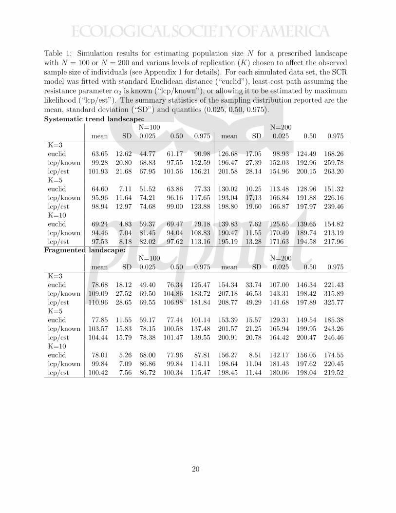
Table 1: Simulation results for estimating population size N for a prescribed landscapewith N = 100 or N = 200 and various levels of replication (K) chosen to affect the observedsample size of individuals (see Appendix 1 for details). For each simulated data set, the SCRmodel was fitted with standard Euclidean distance (“euclid”), least-cost path assuming theresistance parameter α2 is known (“lcp/known”), or allowing it to be estimated by maximumlikelihood (“lcp/est”). The summary statistics of the sampling distribution reported are themean, standard deviation (“SD”) and quantiles (0.025, 0.50, 0.975).Systematic trend landscape:

N=100 N=200mean SD 0.025 0.50 0.975 mean SD 0.025 0.50 0.975

K=3euclid 63.65 12.62 44.77 61.17 90.98 126.68 17.05 98.93 124.49 168.26lcp/known 99.28 20.80 68.83 97.55 152.59 196.47 27.39 152.03 192.96 259.78lcp/est 101.93 21.68 67.95 101.56 156.21 201.58 28.14 154.96 200.15 263.20K=5euclid 64.60 7.11 51.52 63.86 77.33 130.02 10.25 113.48 128.96 151.32lcp/known 95.96 11.64 74.21 96.16 117.65 193.04 17.13 166.84 191.88 226.16lcp/est 98.94 12.97 74.68 99.00 123.88 198.80 19.60 166.87 197.97 239.46K=10euclid 69.24 4.83 59.37 69.47 79.18 139.83 7.62 125.65 139.65 154.82lcp/known 94.46 7.04 81.45 94.04 108.83 190.47 11.55 170.49 189.74 213.19lcp/est 97.53 8.18 82.02 97.62 113.16 195.19 13.28 171.63 194.58 217.96

Fragmented landscape:N=100 N=200

mean SD 0.025 0.50 0.975 mean SD 0.025 0.50 0.975

K=3euclid 78.68 18.12 49.40 76.34 125.47 154.34 33.74 107.00 146.34 221.43lcp/known 109.09 27.52 69.50 104.86 183.72 207.18 46.53 143.31 198.42 315.89lcp/est 110.96 28.65 69.55 106.98 181.84 208.77 49.29 141.68 197.89 325.77K=5euclid 77.85 11.55 59.17 77.44 101.14 153.39 15.57 129.31 149.54 185.38lcp/known 103.57 15.83 78.15 100.58 137.48 201.57 21.25 165.94 199.95 243.26lcp/est 104.44 15.79 78.38 101.47 139.55 200.91 20.78 164.42 200.47 246.46K=10euclid 78.01 5.26 68.00 77.96 87.81 156.27 8.51 142.17 156.05 174.55lcp/known 99.84 7.09 86.86 99.84 114.11 198.64 11.04 181.43 197.62 220.45lcp/est 100.42 7.56 86.72 100.34 115.47 198.45 11.44 180.06 198.04 219.52

20

LIST OF FIGURES:396

Figure 1: Typical home ranges for 4 individuals in the fragmented landscape. The black397

dot indicates the home range center and the cells around each home range center are shaded398

according to the probability of encounter, if a trap were located in that cell.399

Figure 2: Two landscape covariates used for simulations. The left image represents a400

systematic trend that might mimic distance from a habitat feature. The right image is401

a patchy covariate generated by spatially correlated noise. A hypothetical realization of402

N = 100 activity centers is superimposed on the left (black dots), along with 16 trap locations403

(red dots).404

21

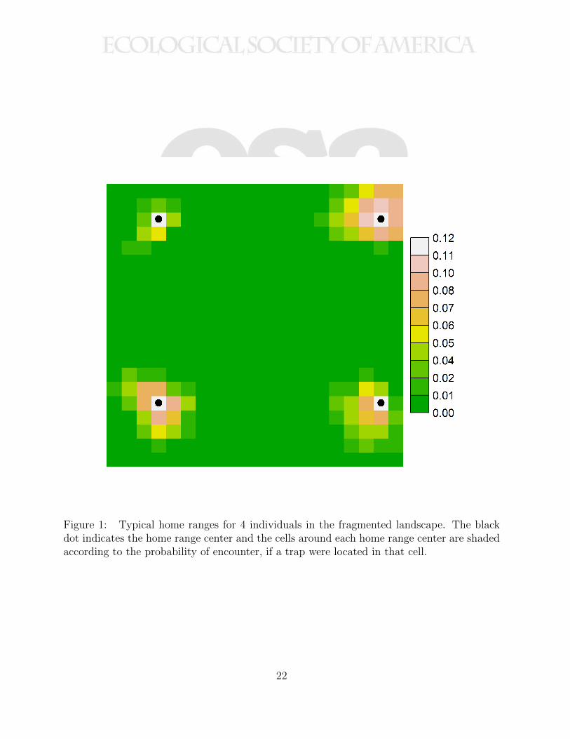
Figure 1: Typical home ranges for 4 individuals in the fragmented landscape. The blackdot indicates the home range center and the cells around each home range center are shadedaccording to the probability of encounter, if a trap were located in that cell.

22

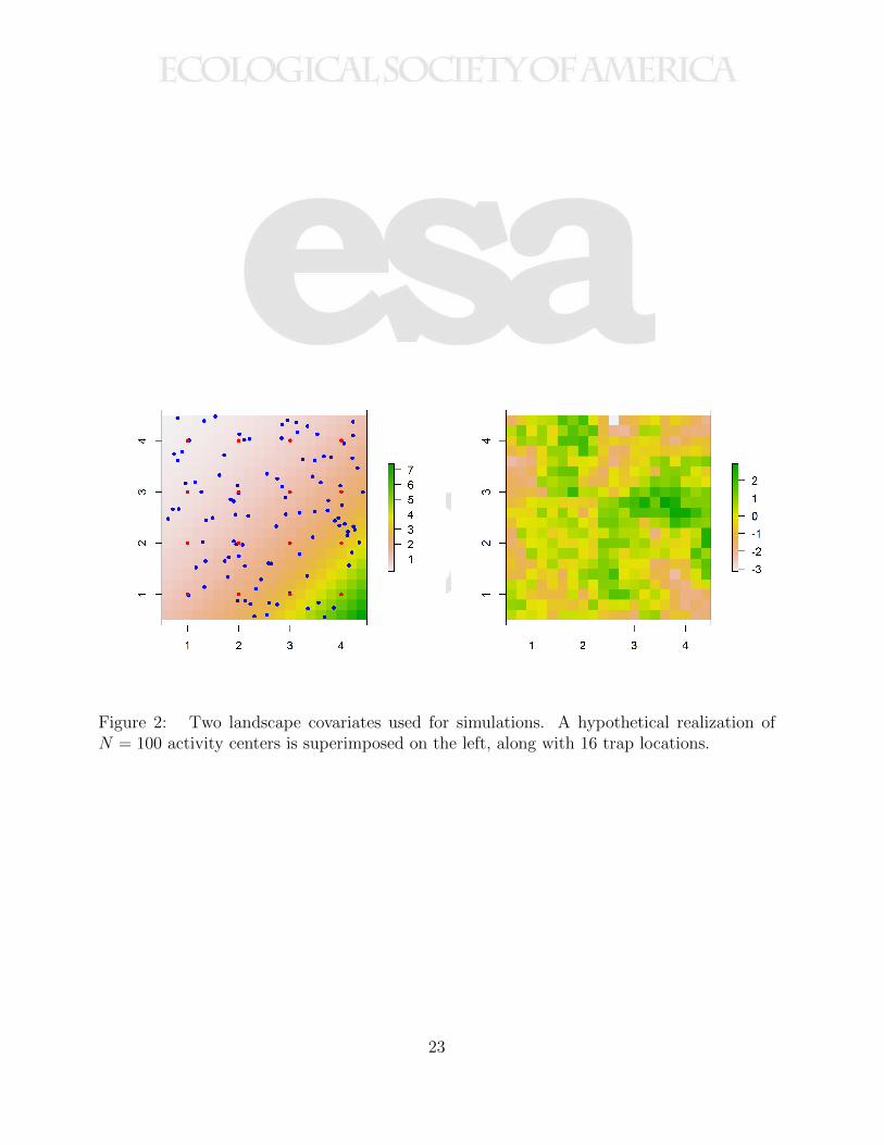
Figure 2: Two landscape covariates used for simulations. A hypothetical realization ofN = 100 activity centers is superimposed on the left, along with 16 trap locations.

23