Spatial Externalities and Vector-Borne Plant Diseases:

Pierce’s Disease and the Blue-Green Sharpshooter in the Napa Valley

Kate Fuller*, Julian Alston**, and James Sanchirico***

* Ph.D. Candidate, Dept. of Ag. and Res. Econ, UC-Davis, fuller@primal.ucdavis.edu

** Professor, Dept. of Ag. and Res. Econ, UC-Davis, julian@primal.ucdavis.edu

***Professor, Dept. of Envr. Sci. and Pol., UC-Davis, jsanchirico@ucdavis.edu

Selected Paper prepared for presentation at the Agricultural & Applied Economics

Association’s 2011 AAEA & NAREA Joint Annual Meeting, Pittsburgh, Pennsylvania,

July 24-26, 2011

©Copyright 2011 by Kate Fuller, Julian Alston, and James Sanchirico. All rights

reserved. Readers may make verbatim copies of this document for non-commercial

purposes by any means, provided that this copyright notice appears on all such copies.

Spatial Externalities and Vector-Borne Plant Diseases:

Pierce’s Disease and the Blue-Green Sharpshooter in the Napa Valley

ABSTRACT: Pierce’s Disease (PD) is a bacterial disease that can kill grapevines over a

span of one to three years. In this paper, we examine and model PD and vector control

decisions made at the vineyard level in the Napa Valley in an effort to understand how

the pest and disease affect individual growers, and to examine spatial externality issues

and potential benefits from cooperation between adjacent vineyards. The model that we

created adds to the literature by (a) treating grape vines as capital stocks that take time to

reach bearing age and thus cannot be immediately replaced in the event of becoming

diseased. We also (b) relax the assumption of an interior solution by examining the

boundaries of parameter space for which winegrape growing is profitable and thus

allowing growers to abandon land if it is not. We also explore (c) the effect of changing

different policy parameters, such as PD control and vine replacement costs. Finally (d)

we examine the potential benefits of cooperation between growers to manage vector

populations, and determine that coordinated vector control could help riparian-adjacent

growers to lessen grapevine losses and land abandonment, and thus to remain profitable

in times of high PD pressure.

Key Words: Pierce’s Disease, winegrapes, perennial crop modeling, agricultural pests

and diseases, optimal control theory

2

Introduction

Pierce’s Disease (PD), caused by a strain of the bacterium Xylella fastidiosa (Xf), was

first reported in California vineyards in the 1880s. PD can kill grapevines over a span of

one to three years by clogging the xylem and thus limiting water transport within the

plant. Today, PD has been identified in grapevines in 28 California counties (California

Department of Agriculture 2009).

In California, PD is spread mainly by sap-feeding insects called sharpshooters.

The relevant species of sharpshooters and the nature of the problems they impose vary

significantly among the major winegrape growing regions of California. In the Napa

Valley, native Blue-Green Sharpshooters (Graphocephala atropunctata, BGSS) have

vectored PD from riparian areas (near streams and rivers) into vineyards for many years.

The problem there is regarded as chronic but manageable, with severity that varies from

year to year. However, some growers have chosen to abandon otherwise exceedingly

valuable land in areas where it is too difficult to control the disease (See Figure 1 for an

aerial image of abandoned or partially-abandoned blocks).

In this paper, we examine and model PD and vector control decisions made at the

vineyard level in the Napa Valley in an effort to understand how the pest and disease

affect individual growers, and to examine spatial externality issues and potential benefits

from cooperation between adjacent vineyards. The model that we created adds to the

literature by (a) treating grape vines as capital stocks that take time to reach bearing age

and thus cannot be immediately replaced in the event of becoming diseased. This builds

directly upon the work of Brown (1997) and Brown, Lynch, and Zilberman (2002) who

considered the same disease in the Napa Valley but did not consider the perennial nature

of grapes. We also (b) relax the assumption of an interior solution by examining the

3

boundaries of parameter space for which winegrape growing is profitable and thus

allowing growers to abandon land if it is not. This issue is of particular interest because

vineyard land in Napa County is some of the most expensive in the world (on average,

between $225,000 and 300,000/acre), and thus abandonment represents a large

opportunity cost (California Chapter of the American Society of Farm Managers and

Rural Appraisers 2010).

We also explore (c) the effect of changing different policy parameters, such as PD

control and vine replacement costs. These numerical explorations could offer insight to

policymakers in times of PD stress, or in the event of the introduction of an exotic vector,

such as the Glassy-Winged Sharpshooter, which has decimated vineyards in southern

parts of the state. Finally (d) we examine the potential benefits of cooperation between

growers to manage vector populations, and determine that coordinated vector control

could help riparian-adjacent growers to lessen grapevine losses and land abandonment,

and thus to remain profitable in times of high PD pressure.

Motivation

The main breeding habitat for BGSSs is in the riparian zone, although irrigated

landscaped areas can also host breeding populations (Pierce's Disease/Riparian Habitat

Workgroup 2000). While some BGSSs will remain in the riparian area throughout their

lifecycle, some adult female sharpshooters leave in the spring and lay their eggs on lush

new growth in surrounding vineyards. Upon hatching, nymphs go through several

moltings before they become winged adults and can leave the plant on which they

hatched. If a BGSS feeds on an infected plant, the bacteria can attach to its mouthparts

4

and colonize there.1 Prior to the adult stage, the BGSSs shed their mouthparts as part of

each molting, but if they do become infected at the adult stage, they will remain so until

their death, and can transmit PD with an efficiency of up to 90 percent upon any given

feeding (Purcell and Finlay 1979).

The flight range for the BGSS is not far; most insects do not travel more than 800

feet from where they hatch. Nevertheless, the damage they inflict in riparian-adjacent

vineyards can be substantial. In interviews we conducted with growers, many individuals

stated that in vineyards near riparian corridors, PD caused major economic losses; some

vineyard managers stated that it was the main reason for abandoning vineyard blocks in

the most seriously affected locations (Grower A 2009; Grower B 2010).2 Figure 1 in

Appendix A shows aerial photos of vineyards with blocks of abandoned land.

In the Napa Valley, one of the main methods of contending with PD is to remove

the riparian plants that harbor breeding populations of the BGSS. One vineyard manager

interviewed stated that the removal of host plants can reduce PD-related vine loss by up

to 90 percent (Grower C 2009). Others did not estimate such high effectiveness, but most

stated that riparian revegetation could yield substantial economic gains, provided that

work in the riparian area was not too difficult because of rocky or steep conditions. Even

under good working conditions, costs associated with revegetation can be significant.

The process of design, approval, and implementation of a riparian revegetation plan can

take over a year to complete (Pierce's Disease/Riparian Habitat Workgroup 2000). To

encourage survival of the new plantings, a drip irrigation system must be installed. Field

interviewees gave estimates of between $5 (Grower C 2009) and $12 per foot of river

1 Plants that harbor PD are not limited to grapevines.

2 Names are suppressed for confidentiality.

5

frontage (Grower A 2009) and beyond (Grower D 2010) for initial costs of revegetating a

stretch of river.

While Napa County produced less than 4 percent of the total volume of the grapes

crushed for wine in California in 2008, the winegrape crush in that year was valued at

nearly $400 million, or over 20 percent of the total crush revenue in the state (California

Department of Agriculture/National Agricultural Statistics Service 2009). Therefore,

while it may be less threatening to the California wine grape industry than other vectors

of PD, such as the newly-arrived invasive Glassy-Winged Sharpshooter that plays a role

in the southern part of the state, growers and policymakers are very concerned about the

damages and corresponding economic losses that the BGSS can cause.

Interviews

To get a better idea of the PD situation in Napa County, we interviewed seven vineyard

managers during February and March of 2010, using a process called “participatory

mapping.” Aiming to glean insight into how PD costs and damages vary among

properties, we asked respondents to sketch onto aerial images of their vineyard blocks

where and how they manage PD and the associated costs. Each interviewee was

presented with two images; one was for a block adjacent to a riparian area, while the

other was as similar as possible in grape variety and clone, but relatively far away from

the riparian zone. Figure 1 in Appendix A shows an example of an aerial image of

vineyard blocks adjacent to the Napa River, onto which a vineyard manager has made

notes regarding PD problems and associated management strategies such as aggressive

replanting (“aggr. replant”) or partial abandonment (“No replant”).

6

A recurring theme in the interviews was the presence of spatial externalities.

Specifically, vineyard managers worried if and how their neighbors were controlling for

PD and how it might affect them. In what follows, we attempt to model those

interactions and to examine how adjacent vineyard managers’ decisions can affect each

other.

Bioeconomic Model of Spatial Pest and Disease Externalities

Many published articles have used optimal control techniques to model the management

of a pest or disease within an agricultural or wildlife setting. To our knowledge, though,

none of these studies used optimal control to model pest and disease management for a

perennial crop.

Several articles in particular have guided our thinking about the bioeconomic

modeling of agricultural pests and diseases. Fenichel and Horan (2007) addressed bovine

tuberculosis in deer populations, and showed that sex-based harvesting strategies can be

an important tool in curbing disease prevalence. Bicknell, Wilen, and Howitt (1999) also

examined bovine tuberculosis, but across different populations: as spread to cattle in

New Zealand by Australian brushtailed possums. They showed the importance of the

disease transmission rate in influencing the sensitivity of cattle farmers to rates of subsidy

for trapping possums. Marsh, Huffaker, and Long (2000) addressed potato leafroll virus

vectored by the green peach aphid, highlighting the influence of weather patterns and

degree-day accumulation on the aphid population size and therefore its ability to vector

the virus. Bhat and Huffaker (2007) used game theory to explore cooperation between

adjacent landowners who face damages from beavers. They showed that the potential

7

economic gains from cooperation are substantial, and are maximized in the scenario in

which the landowners have the greatest flexibility in the extent of their cooperation.

Additional studies have considered the spatial spread of vectors, specifically for

PD as vectored by the BGSS in the Napa Valley wine industry, but have not addressed

the perennial nature of the crop. Brown, Lynch, and Zilberman (2002) emphasized

disease transmission and source control for dealing with the problem.3 The authors

considered riparian plant removal, but focused mainly on barrier methods. This pest

control method reduces the transmission of the disease from the riparian area into the

vineyard by placing an obstruction between the source habitat and the vineyard. The

authors assumed that vineyard managers would grow a barrier of Christmas trees, and

that these trees could be sold. They modeled disease prevalence as a function of the

effectiveness of the barrier in preventing the insects from moving into the vineyard, with

the spread of the disease determined by the width and effectiveness of the barrier. The

authors used these components to create a social decision problem with choice variables

including (a) the width of the barrier; (b) input use; and (c) the extent of removal of

source vegetation.

Brown (1997) modeled the decision of whether to remove riparian plants in

greater detail. At the time of the study, riparian revegetation was not an option because

of laws governing riparian areas, but Brown examined decisions regarding revegetation if

it were legalized. She estimated that costs of removal and revegetation would have to be

greater than $42 per foot to induce a profit-maximizing grower to choose not to undertake

3 The authors ignored pesticide use because, at the time of the article’s publication, only one pesticide

(Dimethoate 400) was permitted for riparian application and it required a special permit. This method of

pest management is now illegal in Napa County. Imidacloprid, the current pesticide of choice for

sharpshooters, was not examined.

8

revegetation. We build on this work by allowing explicitly for the perennial crop

characteristics, which mean that loss of vines involves economic losses over multiple

years. Considering the perennial nature of the crop may be especially important because

it implies that grapevines should be treated as a capital stock.

A Basic Model

In this section we describe a bioeconomic model and the results from applying it to

examine growers’ decisions about PD control under a variety of scenarios defined in

terms of the number of growers and the extent of their cooperation. We have created a

basic model in which we use optimal control to define parameterized solutions for three

scenarios: 1) a single isolated grower, 2) two growers, one of whom controls unilaterally,

taking the neighbor’s insect population (and therefore dispersal) as given, and 3) a social

planner who maximizes the joint profit of multiple blocks with inter-block sharpshooter

migration.

What follows is a basic model of a pest or disease that spreads over space and

affects a perennial crop. We present this model in reference to PD in the Napa Valley,

although it is applicable to other pests and diseases that affect perennials over multiple

seasons. Let Ni represent the insect population on grower i's land. Nj represents the

insect population on i’s neighbors’ properties, N1, N2,…, Ni-1, Ni+1,…NM. Ii represents

the number of vines bought to replace those killed by disease and natural death, and Yi is

i's yield per vine that is healthy and has reached bearing age. NB

iA and B

iA represent the

numbers of non-bearing and bearing vines, respectively. The cost functions for control

and investment are expressed as wS(Si)

and w

I(Ii), respectively. The price per ton of the

9

grapes crushed is represented by p. iS is the quantity of individual i’s control. Each

grower chooses Si and Ii to solve the following problem over a given time period, where ρ

is the discount rate.

(1) , ,

S I

0max p Y w ( ) w ( )

I S N

B t

i i iA S I e dt

This maximization problem is subject to several constraints in the form of

differential equations. The equation of motion for the insect population is:

(2) 2

i,j

RR β δ

K

I

i i i i i j

j i

N N N N S N

,

where R measures sharpshooter intrinsic growth rate, K is a measure of the carrying

capacity of the insect population, β measures the effectiveness of the control, and i,jδ ,

( i,jδ 0 ) is the entry from the i

th row and the j

th column of the MxM dispersal matrix,

where M is the total number of growers. The change in non-bearing and bearing

vinestocks, NB

iA and B

iA , also are defined by differential equations. Each stock has a

separate equation; since grapevines take between three and five years to reach bearing

age, it is not possible for growers to buy replacement vines that will bear immediately.4

The vines are modeled as capital stocks and the pest causes a loss of capital, a departure

from annual crop models in which the pest causes a loss of yield in current production ().5

(3)

NBμ dNB NB NB

i i i i iA I A A N

4 Pierce’s Disease kills the entire grapevine, including the root system. Therefore, grafting is not an option

for vine replacement.

5 Note that the control can also be structured to reduce insect carrying capacity, which would more

accurately reflect the case of riparian revegetation. This is easily accomplished by allowing the control to

change the relationship of R and K. Results are available in which we conducted analyses in this fashion. However, the two sets of results are not substantively different, and the model above allows greater

generality since it could apply to either pesticide application or riparian revegetation.

10

(4) Bμ d ηB NB B B

i i i i iA A A N A

The parameter dj, j=NB, B, measures the damage to the non-bearing or bearing stock,

respectively, that is caused by each insect. The percentage of vines that mature from non-

bearing to bearing each year is represented by μ, and η represents the percentage of vines

that die of natural causes each year. Additionally, the total number of vines that grower i

can have is constrained by the total amount of land in a given block, Ai, which can be

greater than the sum of all planted acres if the grower chooses to leave some land fallow.

In (5) a i converts vines to acres (its units are acres/vine).

(5) A a ( )NB B

i i i iA A

Social Planner Case

The social planner aims to maximize the sum of profits across all landowners on the

riparian strip, i=1,…,M. Because the land constraint does not vary over time, we write

the problem as a Lagrangian instead of a Hamiltonian (Kamien and Schwartz 1991). The

Lagrangian in the social planner case, assuming quadratic cost functions, can be written

as:

(6)

2 2 NB

0 1 0 1

B

1

2

i,j

1

p Y w w w w μ d

μ d η a

RR β δ

K

B S S I I NB NB NB

i i i i i i i i i

MB NB B B A NB B

i i i i i i i

i

I

i i i i i j

j

A S S I I I A A N

L A A N A A A A

N N N S N

.

11

Assuming an interior solution, the optimal control first-order conditions on the control

variables, S and I, are given in Equations (7) and (8).6 At the optimum, the marginal cost

of vine replacement is equal to the shadow value of a non-bearing vine, and the marginal

cost of an additional unit of control is equal to the value of the marginal damage, which is

positive since i <0.

(7)

1 0w w 0I I NB

i i

i

LI

I

, or,

1 0w +wI I NB

i iI

(8) 1 0w w 0,S S

i i i

i

LS N

S

or,

1 0w +w .S S

i i iS N

Taking derivatives of the Lagrangian with respect to the shadow values gives us

back the equations of motion. To allow for land abandonment in the land constraint, we

use Kuhn-Tucker conditions:

(9) 0.A

i

L

If (9) is strictly negative, land is abandoned, and 0A

i . If, instead, A

i > 0, then (9)

must equal zero, with all land planted in vines (Kamien and Schwartz 1991). Note that

the derivative of (5) also implies that when absent abandonment,

(10) B NB

i iA A ,

meaning that the change in the stock of bearing vines is equal to the negative of the

change in the non-bearing vines, Alternatively, with some abandonment,

(11) aAband NB B

i i iA A A ,

6 Chiang (1992) showed that additional state-space equations must be satisfied to check the robustness of

the solution when there are constraints on the state variables that do not include the control variable.

12

meaning that any change in one of the bearing, nonbearing, or abandoned acreage stocks

is equal to the negative of the combined change in acreage of the others.

The full system of equations is rounded out by the costate conditions, some of

which we have omitted here to conserve space.

(12) ρ i i

i

L

N

1

Rρ d d R 2 ,or,

K

NNB NB NB B B B

i i i i i i i i i j ji

j

A A N S

1

Rd +d R 2 ρ .

K

NNB NB NB B B B

i i i i i i i i j ji

j

A A N S

The insect population costate equation, (12), is interpreted such that that any change in

the value of damage caused by sharpshooters is a function of the shadow value of vines

lost to PD and the current shadow value of insects adjusted for the marginal productivity

of the insect and discounting, as well as dispersal; growers take into account the insects

that leave their properties ( δ ii ).

For one isolated grower, the sole difference in the model is that the dispersal term

drops out. Thus (12) becomes

(12a) R

d +d R 2 ρ ,K

NB NB NB B B B

i i i i i i i iA A N S

and thus the isolated grower takes into account only the damage resulting from the insects

on his own property. Only his own control decisions affect the number of insects in his

vineyard.

13

Non-Cooperative Case

The ways in which the different growers interact can vary, and a scenario in which a

social planner benevolently organizes them is extremely rare. Following Janmaat (2005),

we explore an alternative situation in which each grower maximizes his own profit

without regard for the effect on his neighbors. The optimization results differ from those

of the social planner in Equation (12).

Solving for Ni and comparing the outcomes from the social planner and non-

cooperative cases in the steady state shows that insect populations will be greater under

the noncooperative regime compared with the social planner regime; in Equation (13)

SP

iN represents the number of BGSSs under the social planner regime, and NC

iN

represents the number under the noncooperative regime. Because δ 0ii and 0i , it

follows that SP

iN NC

iN by a difference of 2Rδ

,K

ii ceteris paribus, or more explicitly:

(13) 2R R ρ β d d

K

NB NB NB B B B

i i i i i i iSP

i

i

S A AN

2R R ρ δ β d d

K

NB NB NB B B B

i i ii i i i i i NC

i

i

S A AN

.

Numerical Results

Because of both the number of constraints and their nonlinear nature, an analytical

solution is not feasible, even for a one-grower case in which dispersal is disallowed for

the purposes of simplification. Instead, we now present numerical analyses for examples

14

of one-grower and multiple-grower or (multiple-block) cases at their steady states.7 The

parameterization of these models is described in Appendix B. While the choices of

parameters were informed by interviews with growers and relevant literature, as well as

discussions with scientists, exact parameter estimates were not readily available in all

cases and therefore the results presented should be thought of as numerical examples

rather than empirical case studies.8

One-Grower Case

If one vineyard represents the entire universe of our interest, dispersal of insects between

different landowners need not be considered. In this case, the grower maximizes

individual profit subject to the same constraints described above, with the exception of

(2), the insect population equation, which drops its i,j

1

δI

j

j

N

term.

To determine the importance of the different parameters in the one-grower case,

we conducted comparative statics using the steady-state solutions of the model over a

range of scenarios. To begin, we looked at the single-grower case in which one isolated

grape grower maximizes profit subject to damage from sharpshooters, but experiences

neither in- nor out-migration of the insects. While this scenario is unlikely in the real

world, it is not impossible given that some vineyards in Napa may be surrounded by land

without BGSS host plants. For example, this could be the case if a given grower was

surrounded by neighbors that had all revegetated their riparian land. We examined the

7 Further analysis could include studying the dynamic path of these solutions to determine whether that

additional level of complexity could lend understanding to the issue. However, in preliminary dynamic

analysis, adding an allowance for adjustments over time had little effect.

15

one-grower optimal outcomes over a range of several parameters: control cost, vine

replacement cost, crush price, and vine maturity rate.

As expected, as we increased the price of control, the optimal quantity of control

fell, and to compensate, the number of vines replaced increased. However, over the

feasible range of control prices, no land was abandoned, because it was still relatively

cheap to replace vines. With less and less control, the number of sharpshooters increased

toward the carrying capacity of the block. With more vines needing to be replaced, the

shadow value of land fell.

Changing the price of vine replacement had more dramatic effects on the results.

As we increased the price of vine replacement, control increased to reduce the required

number of vines being replaced. Once vine replacement became too expensive, at

roughly $150/vine (less with a higher discount rate), both control and vine replacement

declined rapidly with additional increases in vine prices, the sharpshooter population

increased, and the grower began to abandon land. For a graphical representation of this

case, see Figure 1.

Comparative statics for the crush price of winegrapes are also of interest. When

we decreased the crush price below $1,200/ton, some land was left fallow, which is

consistent with statements of some growers in interviews who reported that low crush

prices in recent years had led them to abandon certain blocks (or parts of blocks). The

entire block (10 acres) was utilized when the crush price reached around $1,200/ton.9 As

the crush price increased, so did the shadow value of marginal land, which was zero until

the crush price rose above $1,200/ton. Additionally, as the crush price increased, more

control was utilized and more vines were replaced, and as a result the number of

9 No land was planted when the crush price was set at zero.

16

sharpshooters on the property fell. When we decreased the crush price and the cost of

vine replacement simultaneously, land abandonment occurred sooner than if either

element were varied on its own.

We also varied, μ , the parameter that measures vine maturation speed, in order to

get a better idea of the importance of treating vines as capital stocks that take time to bear

fruit, in contrast to annual crops. While this is not a parameter that policymakers have

control over, it can help us to understand the effects of treating grapevines as annuals

rather than capital stocks that take several years to mature. As the speed at which vines

mature was increased, so too did the shadow value of land, the optimal sharpshooter

population, the number of bearing vines, the amount of vines replaced, and the quantity

of control. Varying μ alone did not influence land abandonment, although slower-

maturing vines in combination with a low crush price or high vine replacement cost

caused more land abandonment than would occur otherwise. Thus, treating vines as an

annual rather than a perennial crop can yield estimates of land value that are overinflated,

and predict less use of control and more vine replacement at the optimum. Mature vines

that take longer to replace are more valuable, and thus more worth protecting, ceteris

paribus.10

The discount rate also played an important role in determining the values of

parameters for which land was abandoned. The default discount rate used here is 3

percent per annum. When we increased the discount rate it caused a substantial drop in

the values of vine replacement cost and crush price for which land abandonment began,

and the value of crush price for which land was abandoned increased. At a 7 percent

10

Note that if vine maturation speed were to change, it is likely that other parameters, such as crush price,

would also change, perhaps in dramatic ways.

17

discount rate, land abandonment began when the vine replacement cost was $65/vine,

roughly 55 percent less than the critical value of $145 using a 3 percent discount rate.

Likewise, using a 7 percent discount rate, land abandonment began at a crush price of

$1,800/ton, a 33 percent increase over the critical crush price of $1,350 that applied for a

discount rate of 3 percent.

Two (Noncooperative) Growers, Unilateral Control

In this case, we examined the optimal actions of a single grower with one

neighbor who does not control. We allowed the neighbor’s insect population to vary and

examined the changes in optimal actions of the grower in question in response to changes

in the given insect populations on the neighbor’s land. Additionally, while we fixed the

sharpshooter carrying capacity on Grower 1’s land at 80, it is possible that a neighbor

could have a higher carrying capacity, so we allowed Nj to reach 120 at its maximum.

We (somewhat arbitrarily) assumed that 30 percent of the each grower’s population

migrates into their neighbor’s vineyard.

As we increased the number of insects on the neighbor’s property, control on

Grower 1’s land became less effective, since it was negated in part by the influx of

sharpshooters from neighboring land. As a result, control fell as the number of insects on

a neighbor’s property increased. As control dropped off and more insects migrated in,

the number of vines replaced increased. Grower 1’s own population of insects increased

toward carrying capacity, and the shadow value of Grower 1’s land fell. However,

Grower 1 did not abandon any land.

When we changed other parameters along with the neighboring sharpshooter

population, the land abandonment results changed. While large numbers of in-migrating

18

insects alone did not cause a grower to abandon land, Figure 3 shows that, in combination

with high vine replacement costs, large numbers of neighboring sharpshooters caused the

grower to abandon land at lower vine replacement costs than otherwise (approximately

$150/vine, depending on the influx of insects).

Social Planner with Two Blocks

Next we assumed that a social planner manages two vineyard blocks, to maximize their

combined profit, with grapes grown on Block 1 fetching half the price of grapes grown

on Block 2. We allowed the sharpshooters to migrate between the two properties in the

same fashion as in the unilateral control case; the difference here is that the planner

determines the control strategy in both blocks, so neither population is taken as given.

This is a frequent scenario in Napa, where individual growers often own and manage

blocks in various locations across the county and beyond, so control over multiple blocks

is common. However, it is also common for different growers to own adjacent blocks of

land, so it is interesting to examine this case in order to determine the possible gains from

cooperation between these growers.

As in the one-grower case, as we increased the price of control, both blocks

utilized less of it and instead substituted more vine replacement. Over the range of

control costs we examined, the social planner always devoted more control to the high-

priced block (Block 2) than the low-priced block (Block 1) since the opportunity costs of

foregone crop were higher in Block 2 than in Block 1. As we increased control costs, the

sharpshooter populations in both blocks increased, but the planner did not abandon land

in either block.

19

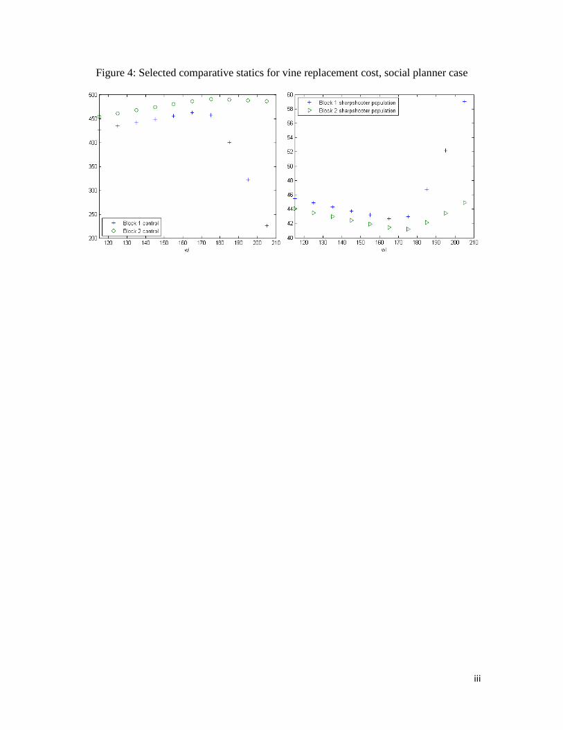
As we increased the price of vine replacement, the planner increased control and

decreased vine replacements. In Block 1, at $170/vine, the marginal shadow value of land

fell to zero, and the social planner began to abandon land. Up until this point, the

increase in control on both blocks led to lower sharpshooter populations, with slightly

fewer sharpshooters in Block 2 than Block 1. After that point, however, control in Block

1 fell and vine replacement dropped drastically. Because control dropped off in Block 1,

the sharpshooter population in that block increased. While the planner did not abandon

land in Block 2 at the same price point as in Block 1, Block 2 began to see increased in-

migration of insects because of the reduction in control in Block 1 and consequently any

control used in Block 2 was less effective. However, the planner did not abandon land in

Block 2 over the relevant parameter space. Note that the price per vine at which land

began to be abandoned is $170, roughly 12 percent higher in the social planner case than

in the two-grower, unilateral control case, supporting the hypothesis that cooperative

control strategies could reduce abandonment. Figure 4 shows control and sharpshooter

population as functions of vine replacement cost for both blocks.

We also experimented with the effects of changing the discount rate for the social

planner case. When we increased the discount rate from 3 to 7 percent per annum, the

planner abandoned land in Block 1 at a lower cost of vine replacement, roughly $65/vine,

or approximately a 40 percent decrease. The planner also abandoned land in Block 2,

although this did not occur until the vine replacement cost reached approximately

$140/vine.

These comparative statics are helpful in showing which parameters have the most

impact as well as in forming testable hypotheses. For example, we expect land adjacent

20

to sharpshooter habitat to be less valuable but land to be worth more if it is next to a

neighbor who does a good job of controlling for sharpshooters. Not surprisingly, we

expect land to be more valuable if it is planted with vines that either mature faster or

fetch a higher crush price.

We also expect high vine replacement cost and/or low crush price to lead growers

to abandon land across a range of scenarios, and a high discount rate will exacerbate land

abandonment in those cases. Perhaps most notably, as long as vines can be replaced

relatively cheaply, land abandonment is fairly insensitive to the cost of control as well as

numbers of in-migrating insects. These could be important pieces of information for

policymakers looking to support grapegrowers during periods of high pressure from PD;

those looking to provide relief to grapegrowers should look to mechanisms that reduce

the price of vine replacement, or compel growers to cooperate regarding their control

schemes.

Conclusions

We constructed this model specifically to examine the Napa Valley/BGSS-

vectored PD issue. In the southern parts of the state, however, the PD problem is quite

different and potentially more threatening to the wine industry there. One potentially

valuable extension of our model might focus on the issue of PD as it affects the

winegrape industry in southern California. Major concerns about PD grew after a

devastating outbreak in the Temecula Valley (in southern California) in the late 1990s,

spread by the newly-arrived, non-native Glassy-Winged Sharpshooter (GWSS), which

has much greater capacity to spread PD than the BGSS because it can fly much longer

21

distances (up to a half mile at a time) and can feed lower on the grape cane. The GWSS

does not depend on riparian or irrigated plants but instead tends to overwinter in citrus

groves, and has the ability to feed on a wide range of plants (Hill 2010). The GWSS

thrives in citrus orchards, which are widespread in southern California. While PD

problems caused by the GWSS in southern California are larger and more difficult to

model in some ways, the spatial externality problem is similar and this could be a useful

extension of the model described here.

In this paper, we have used spatially-explicit modeling techniques to gain a better

understanding of how grapegrowers’ actions indirectly cause them to interact with each

other through their sharpshooter populations. We carefully take account of the biological

characteristics of the insects as well as the perennial nature of the crop being examined,

which both represent differences from other attempts to examine this disease in particular

and other pest and disease problems in agriculture. This work shows how these

characteristics, in concert, can cause growers to abandon land that is affected by the

disease, shedding light on a little understood issue in the Napa Valley. Specifically, we

used a weak inequality constraint to model the constraint on total available land, which

allowed us to explore land abandonment. While the introduction of this seemingly

simple tweak to the classic optimal control model complicated the process of obtaining

solutions, it also showed the importance of doing so in this case as it helps to show why

land is being abandoned in the Napa Valley, an area that contains by far the most

valuable vineyard land in the California (California Chapter of the American Society of

Farm Managers and Rural Appraisers 2010).

22

The results of the numerical analyses can be used to guide policymakers in aiding

grape growers in times of high PD pressure. These results suggest that if heterogeneous

growers can work together to coordinate BGSS control, they will be better off in that they

will experience less damage from PD and will abandon less land. In times of high PD

pressure, policymakers could create pest control districts in which growers (and

residential property owners alike) would be required to treat for BGSS, which could help

curb losses. Additionally, by varying the vine maturation rate, we found that it is

important to consider the perennial, capital stock nature of the grapevines. When we

allowed the vines in the model to mature immediately, as in the annual crop case, the vine

replacement costs for which land was abandoned were much higher, as was the estimate

of the shadow value of land. Our numerical analysis also indicates that some parameters

can be much more useful than others in determining the viability of a vineyard. The price

of vine replacement, in particular, stands out as an important parameter in determining

whether vineyards are profitable. Thus, subsidies on winegrape plantings would be much

more efficient than subsidizing controls or other inputs in assisting grapegrowers in times

of high-PD stress.

i

Appendix A: Tables and Figures

Figure 1: Images of Pierce’s Disease

1a. Diseased Vine and example of land abandonment in the Napa Valley

1b. Participatory Mapping Example

ii

Figure 2: Selected comparative statics for vine replacement cost, one grower case

Figure 3: Abandoned land as a function of vine replacement cost and neighbor’s

sharpshooter population

iii

Figure 4: Selected comparative statics for vine replacement cost, social planner case

i

Appendix B: Model Parameterization

Table 1 summarizes the parameters that we used in the model. The values

assigned were chosen by reviewing the relevant literature as well as consulting experts.

As a result, we have a reasonable amount of confidence in the estimates used, but in some

cases they should be viewed as best guesses rather than statements of fact. The numerical

analysis was conducted using the TOMLAB package in MATLAB using both the knitro and

snopt solvers.

The cost of control is measured by the parameter wS, with the total control cost

being quadratic in controls, S S 2w 0.01wS S . In the base case, we used wS = 6, which

was chosen by speaking with grape growers during interviews about riparian revegetation

as well as alternative control strategies. The cost of vine replacement is structured

similarly, with the total cost equal to 2I 0.01 II Iw w . The base cost of $11/vine was taken

from both interviews with farmers and the Cabernet Sauvignon Vine Loss Calculator for

Napa (Klonsky and Livingston 2009).

For several of the biological parameters we utilized, exact measures were not

available. To estimate these parameters, we discussed them with Barry Hill, the CDFA

entomologist and then conducted sensitivity analyses, many of which are described in the

body of the paper. These include the kill rate, β,and the damage parameter, d, which can

be interpreted as the probability that any one insect will cause disease in a given vine. At

this time we have assumed for simplicity that the rate of damage to non-bearing and

bearing stocks is the same, although the model is written so that these could be different

rates. The sharpshooters’ natural growth rate, R, and measure of carrying capacity, K,

ii

were determined in the same fashion. Note that the carrying capacity is reached at

0N R 1N

N NK

, so K 80N . The dispersal matrix is based on the same

methods. We have assumed at this point that no one grower represents a sink (more

insects enter than exit her property) or a source (more insects exit than enter her

property); instead in our model the properties are fully integrated and insects migrate in

both directions.

We utilized quantity and acreage (to calculate yields) and crush prices from

(rounded) historical averages for Cabernet Sauvignon in the Napa Valley, using the 2009

Crush and Acreage Reports (California Department of Agriculture/National Agricultural

Statistics Service 2009), and the number of vines per acre was taken from (Klonsky and

Livingston 2009). The block acreage ( A ) was in the range of block sizes that growers in

Napa County reported. The rate of vine maturity, μ , is based on vines that reach

maturity at 5 years, which was typical for growers interviewed. In order to avoid

explicitly adding time-lags into an already continuously dynamic model, we assume that

since vines can be replaced each year, 0.2 of all of these non-bearing (immature) vines

become bearing (mature) each year. The non-PD death rate is based on interviews with

farmers.

iii

Table 1: Base Level Parameter Values and Explanations

Parameter Explanation Given value

wS Unit cost of control ($/unit) 6

wI Unit cost of investment ($/vine) 11

dNB

Damage per insect per vine for non-bearing vines 0.0001

dB Damage per insect per vine for bearing vines 0.0001

R Natural growth rate of sharpshooter population 2

K Sharpshooter carrying capacity 80

β Proportion of insects killed per unit of control 0.001*R

Y Yield/vine (tons) 0.00382

a Acres/vine (acres) 1/1555

A Scale unit at which the problem is solved (acres) 10

ρ Annual discount rate 0.03

μ Annual rate of vine maturity from non-bearing to

bearing

0.2

η Annual non-PD death rate 0.02

p Crush price in the one-grower model ($/ton) 4000

p1 Crush price for Block 1 in two grower model ($/ton) 3500

p2 Crush price for Block 2 in two grower model ($/ton) 7000

ij Dispersal between properties; symmetric. 0.3

References:

Bhat, Mahadev, and Ray Huffaker. 2007. Management of a transboundary wildlife

population: A self-enforcing cooperative agreeement with renegotiation and

variable transfer payments. Journal of Environmental Economics and

Management 53:54-67.

Bicknell, Kathryn, James Wilen, and Richard Howitt. 1999. Public policy and private

incentives for livestock disease control. The Australian Journal of Agricultural

and Resource Economics 43 (4):501-521.

Brown, Cheryl. 1997. Three Essays on Issues of Agricultural Sustainability, Agricultural

and Resource Economics, University of California, Berkeley.

Brown, Cheryl, Lori Lynch, and David Zilberman. 2002. The Economics of Controlling

Insect Transmitted Plant Diseases. American Journal of Agricultural Economics

84 (2):279-291.

California Chapter of the American Society of Farm Managers and Rural Appraisers.

2010. Trends in Land and Lease Values. Woodbridge, CA.

California Department of Agriculture. 2009. Pierce’s Disease Control Program 2009

[cited 8 March 2009]. Available from http://www.cdfa.ca.gov/pdcp.html.

California Department of Agriculture/National Agricultural Statistics Service. 2009.

Annual Acreage Report. Sacramento: National Agricultural Statistics California

Field Office.

California Department of Agriculture/National Agricultural Statistics Service. 2009.

Annual Crush Report. Sacramento: National Agricultural Statistics California

Field Office.

Fenichel, Eli, and Richard Horan. 2007. Gender-Based Harvesting in Wildlife Disease

Management. American Journal of Agricultural Economics 89 (4):904-920.

Grower A. 2009. Napa, CA.

Grower B. 2010. Napa, CA.

Grower C. 2009. Napa, CA.

Grower D. 2010. Napa, CA.

Hill, Barry. 2010. Sacramento, CA.

Janmaat, Johannus. 2005. Sharing clams:tragedy of an incomplete commons. Journal of

Environmental Economics and Management 49:26-51.

Kamien, Morton, and Nancy Schwartz. 1991. Dynamic optimization : the calculus of

variations and optimal control in economics and management. Vol. 31, Advanced

Textbooks in Economics. Amsterdam: Elsevier North Holland.

Klonsky, Karen, and Pete Livingston. 2009. Cabernet Sauvignon Vine Loss Calculator.

Davis, CA: University of California.

Marsh, Thomas, Ray Huffaker, and Garrell Long. 2000. Optimal Control of Vector-

Virus-Plant Interactions: The Case of Potato Leafroll Virus Net Necrosis.

American Journal of Agricultural Economics 82 (3):556-569.

Pierce's Disease/Riparian Habitat Workgroup. 2000. Riparian Vegetation Management

for Pierce’s Disease in North Coast California Vineyards. Berkeley: University of

California.

Purcell, Alexander, and Alexander Finlay. 1979. Evidence for Noncirculative

Transmission of Pierce’s Disease bacterium by sharpshooter leafhoppers.

Phytopathology 69 (5):393-395.