Embed Size (px)
Citation preview
Article
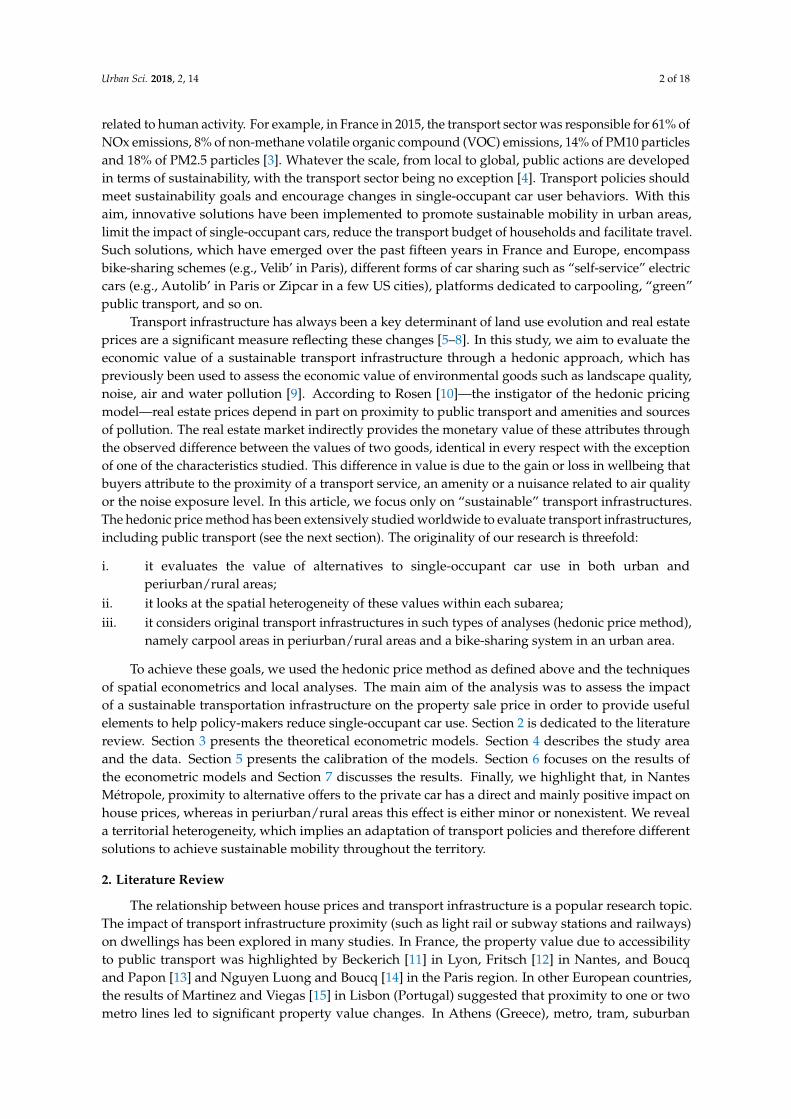
Spatial Heterogeneity of Sustainable TransportationOffer Values: A Comparative Analysis of NantesUrban and Periurban/Rural Areas (France)
Julie Bulteau 1,*, Thierry Feuillet 2 and Rémy Le Boennec 3
1 Department of Economy, Université de Versailles Saint-Quentin, OVSQ, CEARC EA 4455,78280 Guyancourt, France
2 Department of Geography, Université de Paris 8, UMR 7533 LADYSS, 93526 Saint-Denis, France;[email protected]
3 VEDECOM Institute and CentraleSupélec, Laboratoire Génie Industriel, Université Paris-Saclay,91190 Gif-sur-Yvette, France; [email protected]
* Correspondence: [email protected]
Received: 3 December 2017; Accepted: 31 January 2018; Published: 7 February 2018
Abstract: Innovative solutions have been implemented to promote sustainable mobility in urbanareas. In the Nantes area (northwestern part of France), alternatives to single-occupant car usehave increased in the past few years. In the urban area, there is an efficient public transportsupply, including tramways and a “busway” (Bus Rapid Transit), as well as bike-sharing services.In periurban and rural areas, there are carpool areas, regional buses and the new “tram-train”lines. In this article, we focus on the impact on house prices of these “sustainable” transportationinfrastructures and policies, in order to evaluate their values. The implicit price of these sustainabletransport offers was estimated through hedonic price functions describing the Nantes urban andperiurban/rural housing markets. Spatial regression models (SAR, SEM, SDM and GWR) werecarried out to capture the effect of both spatial autocorrelation and spatial heterogeneity. The resultsshow patterns of spatial heterogeneity of transportation offer implicit prices at two scales: (i) betweenurban and periurban/rural areas, as well as (ii) within each territory. In the urban area, the distanceto such offers was significantly associated with house prices. These associations varied by typeof transportation system (positive for tramway and railway stations and negative for bike-sharingstations). In periurban and rural areas, having a carpool area in a 1500-m buffer around the homewas negatively associated with house prices, while having a regional bus station in a 500-m bufferwas non-significant. Distance to the nearest railway station was negatively associated with houseprices. These findings provide research avenues to help public policy-makers promote sustainablemobility and pave the way for more locally targeted interventions.
Keywords: sustainable mobility; transport accessibility; geographically weighted regression; hedonicpricing method; spatial dependence; spatial heterogeneity
1. Introduction
To become a sustainable city or, more broadly, to develop a sustainable territory, has becomea major challenge of our societies. Rethinking the organization of our cities, and thus changing thetraditional planning models, is one of the priorities of public policies [1]. This involves promotingsustainable infrastructures and especially offering alternatives to the single-occupant car. In France in2014, the transport sector was considered the main source of greenhouse gas emissions, representingslightly less than 30% of the national emissions. Moreover, these transport-related emissions increasedsignificantly (+20%) between 1990 and 2001 [2]. Concerning the local pollution, most air pollutants were
Urban Sci. 2018, 2, 14; doi:10.3390/urbansci2010014 www.mdpi.com/journal/urbansci
Urban Sci. 2018, 2, 14 2 of 18
related to human activity. For example, in France in 2015, the transport sector was responsible for 61% ofNOx emissions, 8% of non-methane volatile organic compound (VOC) emissions, 14% of PM10 particlesand 18% of PM2.5 particles [3]. Whatever the scale, from local to global, public actions are developedin terms of sustainability, with the transport sector being no exception [4]. Transport policies shouldmeet sustainability goals and encourage changes in single-occupant car user behaviors. With thisaim, innovative solutions have been implemented to promote sustainable mobility in urban areas,limit the impact of single-occupant cars, reduce the transport budget of households and facilitate travel.Such solutions, which have emerged over the past fifteen years in France and Europe, encompassbike-sharing schemes (e.g., Velib’ in Paris), different forms of car sharing such as “self-service” electriccars (e.g., Autolib’ in Paris or Zipcar in a few US cities), platforms dedicated to carpooling, “green”public transport, and so on.
Transport infrastructure has always been a key determinant of land use evolution and real estateprices are a significant measure reflecting these changes [5–8]. In this study, we aim to evaluate theeconomic value of a sustainable transport infrastructure through a hedonic approach, which haspreviously been used to assess the economic value of environmental goods such as landscape quality,noise, air and water pollution [9]. According to Rosen [10]—the instigator of the hedonic pricingmodel—real estate prices depend in part on proximity to public transport and amenities and sourcesof pollution. The real estate market indirectly provides the monetary value of these attributes throughthe observed difference between the values of two goods, identical in every respect with the exceptionof one of the characteristics studied. This difference in value is due to the gain or loss in wellbeing thatbuyers attribute to the proximity of a transport service, an amenity or a nuisance related to air qualityor the noise exposure level. In this article, we focus only on “sustainable” transport infrastructures.The hedonic price method has been extensively studied worldwide to evaluate transport infrastructures,including public transport (see the next section). The originality of our research is threefold:
i. it evaluates the value of alternatives to single-occupant car use in both urban andperiurban/rural areas;
ii. it looks at the spatial heterogeneity of these values within each subarea;iii. it considers original transport infrastructures in such types of analyses (hedonic price method),
namely carpool areas in periurban/rural areas and a bike-sharing system in an urban area.
To achieve these goals, we used the hedonic price method as defined above and the techniquesof spatial econometrics and local analyses. The main aim of the analysis was to assess the impactof a sustainable transportation infrastructure on the property sale price in order to provide usefulelements to help policy-makers reduce single-occupant car use. Section 2 is dedicated to the literaturereview. Section 3 presents the theoretical econometric models. Section 4 describes the study areaand the data. Section 5 presents the calibration of the models. Section 6 focuses on the results ofthe econometric models and Section 7 discusses the results. Finally, we highlight that, in NantesMétropole, proximity to alternative offers to the private car has a direct and mainly positive impact onhouse prices, whereas in periurban/rural areas this effect is either minor or nonexistent. We reveala territorial heterogeneity, which implies an adaptation of transport policies and therefore differentsolutions to achieve sustainable mobility throughout the territory.
2. Literature Review
The relationship between house prices and transport infrastructure is a popular research topic.The impact of transport infrastructure proximity (such as light rail or subway stations and railways)on dwellings has been explored in many studies. In France, the property value due to accessibilityto public transport was highlighted by Beckerich [11] in Lyon, Fritsch [12] in Nantes, and Boucqand Papon [13] and Nguyen Luong and Boucq [14] in the Paris region. In other European countries,the results of Martinez and Viegas [15] in Lisbon (Portugal) suggested that proximity to one or twometro lines led to significant property value changes. In Athens (Greece), metro, tram, suburban

Urban Sci. 2018, 2, 14 3 of 18
railway and bus stations affected dwelling prices positively, while ISAP (the old urban railway of Attica)and national rail stations, airports and ports had a negative effect due to a number of externalitiesassociated with them, such as noise [7]. In the United States, Bowes and Ihlanfeldt [16] found bothpositive and negative effects of rail stations on the local house prices in Atlanta. Several other studiesconducted in the USA showed a positive relationship between property values and the distance fromlight rail (LRT) stations, such as in Santa Clara (California) [17,18], Charlotte (North Carolina) [6],Buffalo (New York) [19], Dallas (Texas) [20], Portland (Oregon) [21] and Phoenix (Arizona) [22].In Brisbane (Australia), Mulley et al. [23] found that being close to a bus rapid transit (BRT) added apremium to the housing price of 0.14% for every hundred meters closer to the BRT station. In Shanghai,the hedonic price modeling of Pan and Zhang [24] showed that the transit proximity premiumamounted to approximately 152 yuan/m2 (about 20 €/m2) for every 100 m closer to a metro station,and Li et al. [25] found similar results in Beijing. Chen and Haynes [26] reported a strong positiveeffect of the Beijing-Shanghai high-speed rail line on housing values, especially in small and mediumcities. In Singapore, Diao et al. [8] found that the opening of an LRT increased housing values withinthe 600 m network distance from the new stations.
Some studies have also explored the relationship between bike facilities and house price.For instance, Liu and Shi [27] underlined that the density of the bike network in Portland (Oregon)was a positive contributor to property values. Welch et al. [21], however, found more mixed resultsin the same city. In Montreal (Canada), El-Geneidy et al. [28] highlighted that the presence of abicycle-sharing system in a neighborhood with 12 stations serving an 800-m buffer was expected toincrease property values by approximately 2.7%. A summary of these literature findings is presentedin Table S1.
3. Presentation of the Econometric Models
3.1. Hedonic Price Model
The objective of the hedonic price method is to reveal the implicit prices of the different attributesof a heterogeneous good on the basis of its overall price. The study of Lancaster [29] laid the theoreticalfoundations of this method and Rosen [10] formalized it. Rosen proposed a two-stage methodin which each stage has limitations that should not be overlooked in an econometric approach.The most common problems are: (i) the failure to take into account the expectations of future levelsof amenities [30]; (ii) the endogeneity of certain explanatory variables, which leads to them beingnot exogenous and correlated with the regression residuals. The OLS estimates then give biased andnon-convergent results [31]. The method of instrumental variables makes it possible to remedy them,and is used in the works of Bartik [31] and Cheshire and Sheppard [32]; and (iii) spatial heterogeneity(variation in housing characteristics and prices across space) and spatial dependence (dependence ofthe housing characteristics and prices in one place on the characteristics of neighboring places).These problems have been highlighted and addressed in many works (e.g., [33,34]).
3.2. Spatial Models
The geolocalized data, i.e., the data for which each observation is associated with a locationidentified by its geographical coordinates (postal addresses of the transactions in our study), requirespecial treatment [34]. Spatial observations are frequently interdependent: what happens in a particularlocation depends on what happens in other locations and refers to the so-called spatial dependence [33].Real estate transactions are no exception. Spatial econometric methods use an instrument to representthese spatial interactions, namely the weight matrix (W) or matrix of the neighbor location datapoints. With N observations, we use a square matrix W (N × N), whose diagonal terms are zero andwhose non-diagonal term wij becomes higher as the effect of observation j on observation i becomeslarger [35]. These matrices are based on either contiguity or distance and are then used to createspatially lagged variables, applicable to the dependent variable, the independent ones, or the error
Urban Sci. 2018, 2, 14 4 of 18
term [7]. These weight matrices can also be based on networks [36]. Specifications of the modelcalibration are given in Section 5.
The spatial econometric model aims are presented as follows:
(1) Spatial AutoRegressive Model (SAR) [37]:
Y = ρWY + Xβ + ε (1)
where Y is the variable explained, X is the matrix of the exogenous variables, ε is an error term,and β is the vector of regression coefficients. The SAR model accounts for a spatial dependenceon the endogenous variable: the price of the house sold (Y) depends on the prices of neighboringhouses, ρ being the spatial parameter to be estimated.
(2) Spatial Error Model (SEM) [37]:
Y = Xβ + ε with ε = λWε + µ (2)
where Y is the variable explained, X is the matrix of the exogenous variables, ε is an error term,and β is the vector of regression coefficients. The SEM model is specified with an autoregressivestructure of the error term, where λ is the spatial parameter to be estimated.
(3) Spatial Durbin Model (SDM) [37]:
Y = ρWY + Xβ + γWX + ε (3)
The SDM model combines the dependence effects on the explanatory variables and on theendogenous variable. The spatial autoregressive process is applied to both the explained andexplanatory variables. ρ and γ are the spatial parameters to be estimated. This model canpotentially remove the bias caused by the omitted variables.
(4) Geographically Weighted Regression (GWR) [38]:
yi = β0(ui, vi) + ∑k
βk(ui, vi)Xik + εi (4)
where (ui,vi) represents the geographical coordinates of location i. The GWR model aims to detectthe spatial heterogeneity of statistical relationships by exhibiting the spatial patterning of localregression coefficients. It extends the traditional regression framework by allowing coefficientsto vary throughout space. One weighted regression is performed per data point, according to aspatial weighting scheme giving more importance to nearer neighbors than farther ones. A keypoint of the GWR model is therefore to calibrate an appropriate kernel function (see Section 5).
4. Study Area and Database
4.1. Nantes Urban and Periurban/Rural Areas
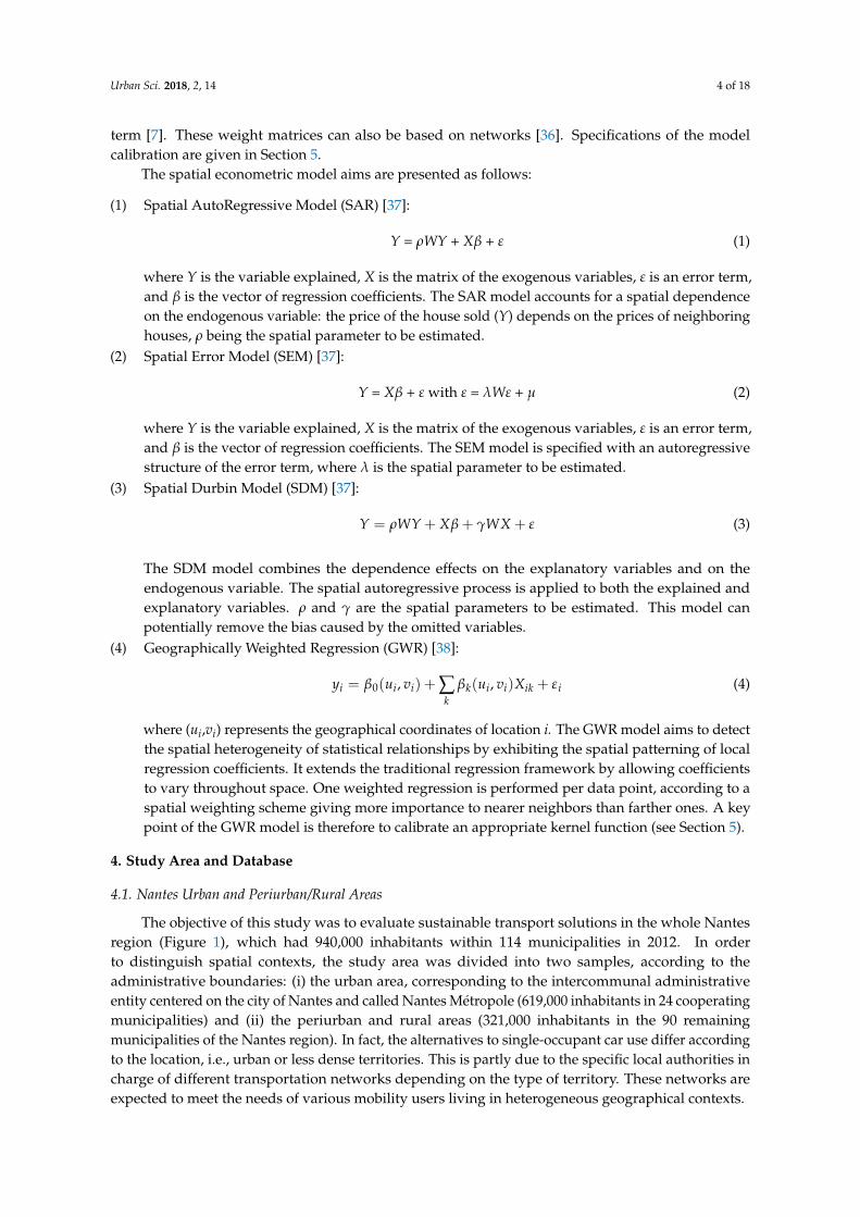
The objective of this study was to evaluate sustainable transport solutions in the whole Nantesregion (Figure 1), which had 940,000 inhabitants within 114 municipalities in 2012. In orderto distinguish spatial contexts, the study area was divided into two samples, according to theadministrative boundaries: (i) the urban area, corresponding to the intercommunal administrativeentity centered on the city of Nantes and called Nantes Métropole (619,000 inhabitants in 24 cooperatingmunicipalities) and (ii) the periurban and rural areas (321,000 inhabitants in the 90 remainingmunicipalities of the Nantes region). In fact, the alternatives to single-occupant car use differ accordingto the location, i.e., urban or less dense territories. This is partly due to the specific local authorities incharge of different transportation networks depending on the type of territory. These networks areexpected to meet the needs of various mobility users living in heterogeneous geographical contexts.

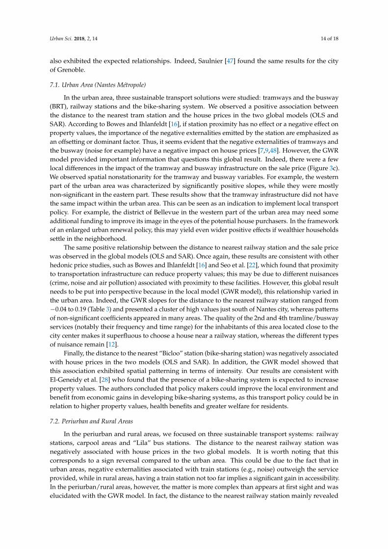
Urban Sci. 2018, 2, 14 5 of 18Urban Sci. 2018, 2, x FOR PEER REVIEW 5 of 18
Figure 1. Location map.
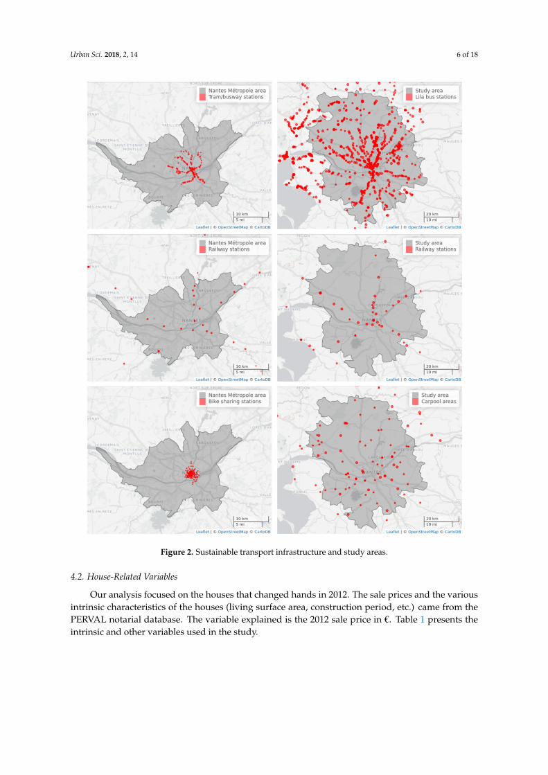
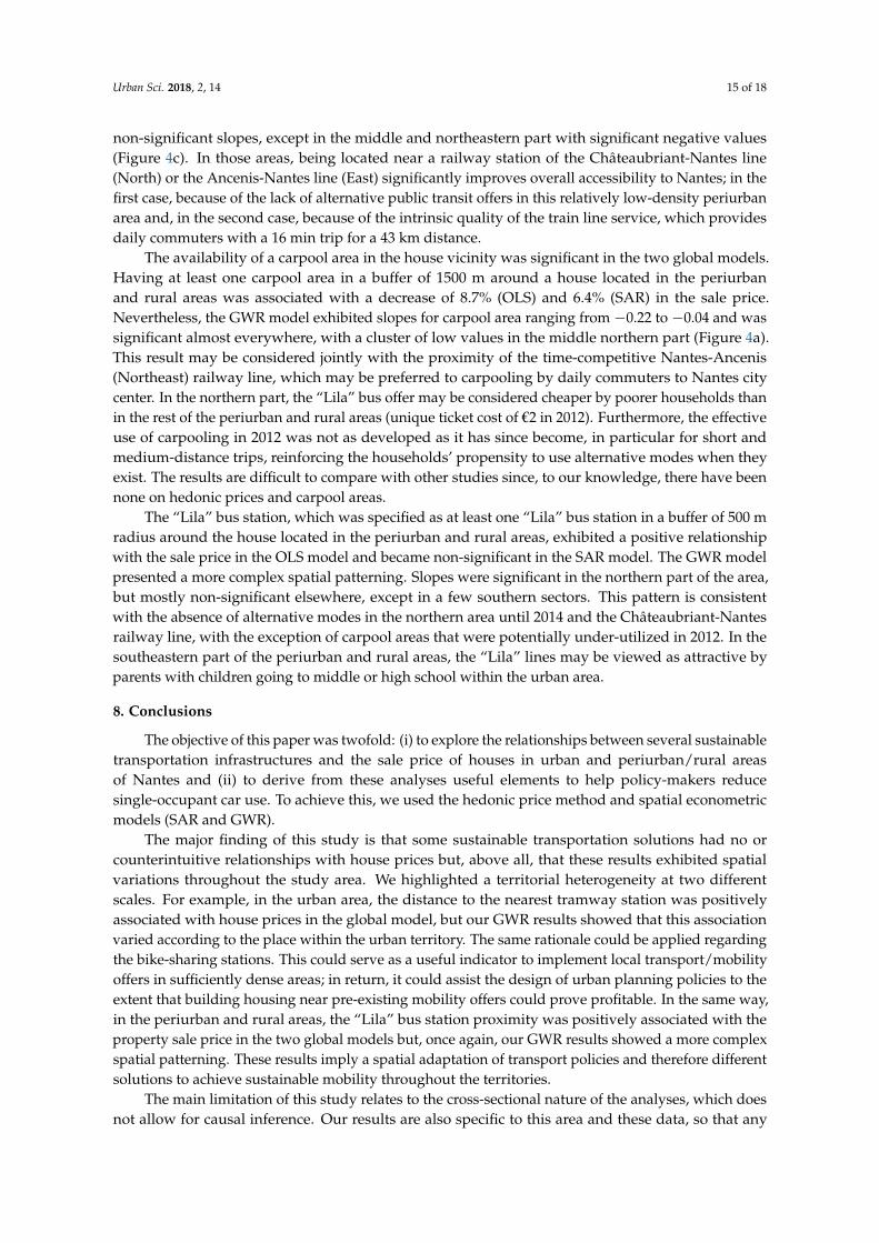
Our study concerned 2262 house transactions, including 1353 in the urban area (Nantes Métropole) and 909 in the periurban and rural areas. In the Nantes urban area (Nantes Métropole), three transportation networks or mobility offers are of interest (Figure 2). The first concerns the location of the 11 railway stations that were in service in 2012. We added the 5 railway stations in the northern part of the urban area (the “tram-train” line from Nantes to Châteaubriant, located 70 km north of Nantes). This specific transport line was opened in February 2014 and was planned by the regional public authority long before 2012; this is why it seemed reasonable to consider that potential accessibility gains provided by this new transport offer could be evaluated in housing prices at this time [39]. The four tramlines were constructed to facilitate radial trips towards Nantes city center using public transport from the rest of the urban area. The first three lines were implemented between 1985 and 2000 while the fourth one (the “busway”, a Bus Rapid Transit or BRT line) was put into service in 2006 as part of the 2000–2010 Urban Transport Plan. The “Bicloo” bike-sharing offer was provided in the central districts of the Nantes urban area in 2008. The station network was gradually extended over a wider territory and included 103 stations in 2012.
The other transportation networks or mobility offers are implemented at the scale of the periurban/rural areas as well as in the Nantes urban area (Figure 2). This is the case of the railway stations along the five train lines leaving Nantes. Many “Lila” bus stations have been implemented in the whole département and within the periurban and rural areas (n = 435). Finally, carpool stations have been either implemented or authorized since 2009 thanks to the contribution of the Loire-Atlantique département.
Figure 1. Location map.
Our study concerned 2262 house transactions, including 1353 in the urban area (Nantes Métropole)and 909 in the periurban and rural areas. In the Nantes urban area (Nantes Métropole),three transportation networks or mobility offers are of interest (Figure 2). The first concerns thelocation of the 11 railway stations that were in service in 2012. We added the 5 railway stations in thenorthern part of the urban area (the “tram-train” line from Nantes to Châteaubriant, located 70 kmnorth of Nantes). This specific transport line was opened in February 2014 and was planned by theregional public authority long before 2012; this is why it seemed reasonable to consider that potentialaccessibility gains provided by this new transport offer could be evaluated in housing prices at thistime [39]. The four tramlines were constructed to facilitate radial trips towards Nantes city centerusing public transport from the rest of the urban area. The first three lines were implemented between1985 and 2000 while the fourth one (the “busway”, a Bus Rapid Transit or BRT line) was put intoservice in 2006 as part of the 2000–2010 Urban Transport Plan. The “Bicloo” bike-sharing offer wasprovided in the central districts of the Nantes urban area in 2008. The station network was graduallyextended over a wider territory and included 103 stations in 2012.
The other transportation networks or mobility offers are implemented at the scale of theperiurban/rural areas as well as in the Nantes urban area (Figure 2). This is the case of therailway stations along the five train lines leaving Nantes. Many “Lila” bus stations have beenimplemented in the whole département and within the periurban and rural areas (n = 435).Finally, carpool stations have been either implemented or authorized since 2009 thanks to thecontribution of the Loire-Atlantique département.
Urban Sci. 2018, 2, 14 6 of 18
Urban Sci. 2018, 2, x FOR PEER REVIEW 6 of 18
Figure 2. Sustainable transport infrastructure and study areas.
4.2. House-Related Variables
Our analysis focused on the houses that changed hands in 2012. The sale prices and the various intrinsic characteristics of the houses (living surface area, construction period, etc.) came from the PERVAL notarial database. The variable explained is the 2012 sale price in €. Table 1 presents the intrinsic and other variables used in the study.
Figure 2. Sustainable transport infrastructure and study areas.
4.2. House-Related Variables
Our analysis focused on the houses that changed hands in 2012. The sale prices and the variousintrinsic characteristics of the houses (living surface area, construction period, etc.) came from thePERVAL notarial database. The variable explained is the 2012 sale price in €. Table 1 presents theintrinsic and other variables used in the study.
Urban Sci. 2018, 2, 14 7 of 18
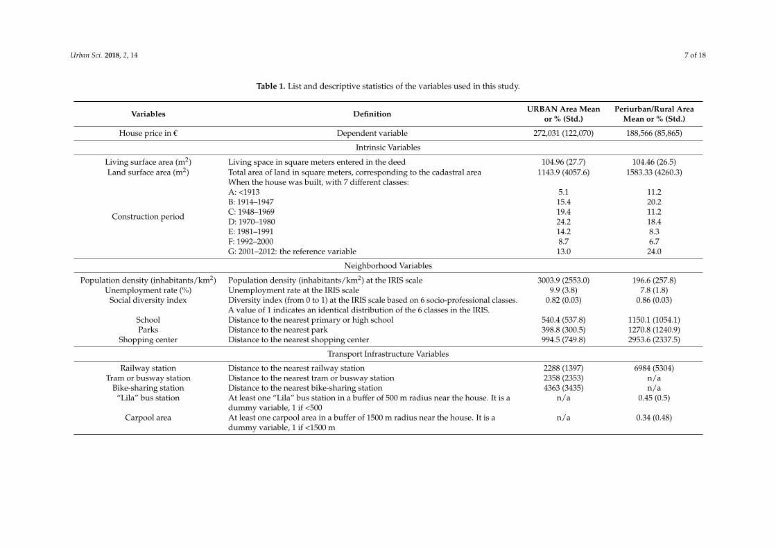
Table 1. List and descriptive statistics of the variables used in this study.
Variables Definition URBAN Area Meanor % (Std.)
Periurban/Rural AreaMean or % (Std.)
House price in € Dependent variable 272,031 (122,070) 188,566 (85,865)
Intrinsic Variables
Living surface area (m2) Living space in square meters entered in the deed 104.96 (27.7) 104.46 (26.5)Land surface area (m2) Total area of land in square meters, corresponding to the cadastral area 1143.9 (4057.6) 1583.33 (4260.3)
Construction period
When the house was built, with 7 different classes:A: <1913 5.1 11.2B: 1914–1947 15.4 20.2C: 1948–1969 19.4 11.2D: 1970–1980 24.2 18.4E: 1981–1991 14.2 8.3F: 1992–2000 8.7 6.7G: 2001–2012: the reference variable 13.0 24.0
Neighborhood Variables
Population density (inhabitants/km2) Population density (inhabitants/km2) at the IRIS scale 3003.9 (2553.0) 196.6 (257.8)Unemployment rate (%) Unemployment rate at the IRIS scale 9.9 (3.8) 7.8 (1.8)
Social diversity index Diversity index (from 0 to 1) at the IRIS scale based on 6 socio-professional classes.A value of 1 indicates an identical distribution of the 6 classes in the IRIS.
0.82 (0.03) 0.86 (0.03)
School Distance to the nearest primary or high school 540.4 (537.8) 1150.1 (1054.1)Parks Distance to the nearest park 398.8 (300.5) 1270.8 (1240.9)
Shopping center Distance to the nearest shopping center 994.5 (749.8) 2953.6 (2337.5)
Transport Infrastructure Variables
Railway station Distance to the nearest railway station 2288 (1397) 6984 (5304)Tram or busway station Distance to the nearest tram or busway station 2358 (2353) n/a
Bike-sharing station Distance to the nearest bike-sharing station 4363 (3435) n/a“Lila” bus station At least one “Lila” bus station in a buffer of 500 m radius near the house. It is a
dummy variable, 1 if <500n/a 0.45 (0.5)
Carpool area At least one carpool area in a buffer of 1500 m radius near the house. It is adummy variable, 1 if <1500 m
n/a 0.34 (0.48)
Urban Sci. 2018, 2, 14 8 of 18
4.3. Spatial Variables
Since the neighborhood characteristics where the dwelling is located might also influencethe sale price, six contextual variables related to the socioeconomic environment and the builtenvironment were added to the models: population density (inhabitants/km2), unemploymentrate (%) and a social diversity index were assessed at the IRIS Census unit scale. The IRIS areas(acronym for “Aggregated Units for Statistical Information”) are provided by the French NationalInstitute of Statistics and Economic Studies (INSEE, www.insee.fr); they represent the smallest unit fordissemination of French infra-municipal data. The social diversity index is a measure of the evennessof distribution of the percentages of six main INSEE-based socio-professional classes (farmers, artisans,managers and higher intellectual professions, intermediate occupations, low-grade white collars,blue collars) in each IRIS. A value of 1 indicates an equal distribution of the six classes in the IRIS.The three other contextual variables characterize the built environment and were computed as thenearest distances of each house to (i) a primary/high school, (ii) a park and (iii) a shopping center.This information is available as shapefiles on the open data webpage of the Loire-Atlantique département(http://data.loire-atlantique.fr/donnees/).
In order to explore the possible impacts on the sale price of infrastructures known as alternatives tosingle-occupant car use, we first assessed the distance between each dwelling and such infrastructures,which vary depending on the sub-area studied. In the urban area (Nantes Métropole), distances to thenearest tram station, railway station and bike-sharing station were used. In the periurban and ruralareas, having at least one “Lila” bus station in a buffer of 500 m radius near the home, one carpoolarea in a buffer of 1500 m radius, and the distance to the railway station were used. These thresholdswere selected according to significance criteria derived from sensitivity analyses (from 250 m to 2000 mfor “Lila” bus stations and from 500 m to 5000 m for carpool areas). Note that the “Lila” bus networkis local public transport mainly dedicated to periurban and rural areas. All these public transportinfrastructures were downloaded as shapefile points from the open data website of the city of Nantes(http://data.nantes.fr/donnees/). Euclidean distances between infrastructure points and dwellingpoints were then calculated. Table 1 presents these sustainable transport-based variables for each typeof territory.
Once the database was built, multicollinearity between regressors was checked through thevariance inflation factor (VIF). No values higher than 4 were present so all the variables were kept.
4.4. Descriptive Statistics
The overall descriptive statistics of the database are given in Table 1. The average sale price was€272,031 for the 1353 houses in the urban area and €188,566 for the 909 houses in the periurban andrural areas, while the average living surface area was quite similar in both spatial contexts (~104 m2).In terms of environmental variables, the population density was approximately 3000 inhabitants/km2
in the urban area and 196 inhabitants/km2 elsewhere, while the unemployment rate was 9.9% and7.8%, respectively. In the urban area, the average distance to the nearest tram/busway station was2358 m, while it was 3788 m to the nearest railway station and 4363 m to the nearest bike-sharingstation. In the periurban and rural areas, 34% of houses included a carpool area in a buffer of 1500 mand 45% a “Lila” bus station in a buffer of 500 m. Finally, the average distance to the nearest railwaystation was 12,580 m.
5. Model Calibration and Selection
The price of the house was retained as the dependent variable. After testing severalmodeling forms, a semi-logarithmic model was chosen. According to Martinez and Viegas [15],this specification usually produces robust estimates and enables convenient coefficient interpretationand is therefore widely used in the property value literature. Independent variables includedhouse intrinsic characteristics, neighborhood variables and sustainable transport attributes.
Urban Sci. 2018, 2, 14 9 of 18
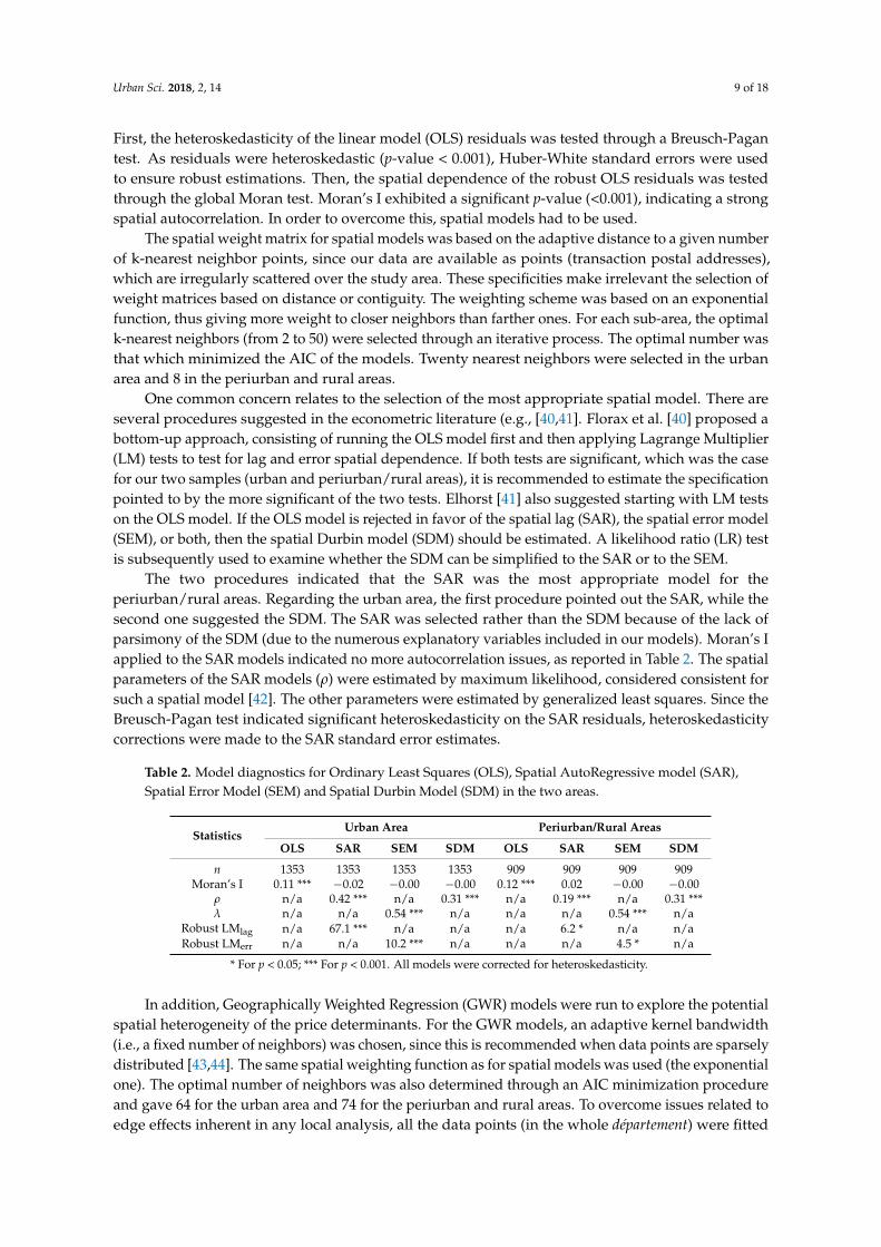
First, the heteroskedasticity of the linear model (OLS) residuals was tested through a Breusch-Pagantest. As residuals were heteroskedastic (p-value < 0.001), Huber-White standard errors were usedto ensure robust estimations. Then, the spatial dependence of the robust OLS residuals was testedthrough the global Moran test. Moran’s I exhibited a significant p-value (<0.001), indicating a strongspatial autocorrelation. In order to overcome this, spatial models had to be used.
The spatial weight matrix for spatial models was based on the adaptive distance to a given numberof k-nearest neighbor points, since our data are available as points (transaction postal addresses),which are irregularly scattered over the study area. These specificities make irrelevant the selection ofweight matrices based on distance or contiguity. The weighting scheme was based on an exponentialfunction, thus giving more weight to closer neighbors than farther ones. For each sub-area, the optimalk-nearest neighbors (from 2 to 50) were selected through an iterative process. The optimal number wasthat which minimized the AIC of the models. Twenty nearest neighbors were selected in the urbanarea and 8 in the periurban and rural areas.
One common concern relates to the selection of the most appropriate spatial model. There areseveral procedures suggested in the econometric literature (e.g., [40,41]. Florax et al. [40] proposed abottom-up approach, consisting of running the OLS model first and then applying Lagrange Multiplier(LM) tests to test for lag and error spatial dependence. If both tests are significant, which was the casefor our two samples (urban and periurban/rural areas), it is recommended to estimate the specificationpointed to by the more significant of the two tests. Elhorst [41] also suggested starting with LM testson the OLS model. If the OLS model is rejected in favor of the spatial lag (SAR), the spatial error model(SEM), or both, then the spatial Durbin model (SDM) should be estimated. A likelihood ratio (LR) testis subsequently used to examine whether the SDM can be simplified to the SAR or to the SEM.
The two procedures indicated that the SAR was the most appropriate model for theperiurban/rural areas. Regarding the urban area, the first procedure pointed out the SAR, while thesecond one suggested the SDM. The SAR was selected rather than the SDM because of the lack ofparsimony of the SDM (due to the numerous explanatory variables included in our models). Moran’s Iapplied to the SAR models indicated no more autocorrelation issues, as reported in Table 2. The spatialparameters of the SAR models (ρ) were estimated by maximum likelihood, considered consistent forsuch a spatial model [42]. The other parameters were estimated by generalized least squares. Since theBreusch-Pagan test indicated significant heteroskedasticity on the SAR residuals, heteroskedasticitycorrections were made to the SAR standard error estimates.
Table 2. Model diagnostics for Ordinary Least Squares (OLS), Spatial AutoRegressive model (SAR),Spatial Error Model (SEM) and Spatial Durbin Model (SDM) in the two areas.
StatisticsUrban Area Periurban/Rural Areas
OLS SAR SEM SDM OLS SAR SEM SDM
n 1353 1353 1353 1353 909 909 909 909Moran’s I 0.11 *** −0.02 −0.00 −0.00 0.12 *** 0.02 −0.00 −0.00
ρ n/a 0.42 *** n/a 0.31 *** n/a 0.19 *** n/a 0.31 ***λ n/a n/a 0.54 *** n/a n/a n/a 0.54 *** n/a
Robust LMlag n/a 67.1 *** n/a n/a n/a 6.2 * n/a n/aRobust LMerr n/a n/a 10.2 *** n/a n/a n/a 4.5 * n/a
* For p < 0.05; *** For p < 0.001. All models were corrected for heteroskedasticity.
In addition, Geographically Weighted Regression (GWR) models were run to explore the potentialspatial heterogeneity of the price determinants. For the GWR models, an adaptive kernel bandwidth(i.e., a fixed number of neighbors) was chosen, since this is recommended when data points are sparselydistributed [43,44]. The same spatial weighting function as for spatial models was used (the exponentialone). The optimal number of neighbors was also determined through an AIC minimization procedureand gave 64 for the urban area and 74 for the periurban and rural areas. To overcome issues related toedge effects inherent in any local analysis, all the data points (in the whole département) were fitted
Urban Sci. 2018, 2, 14 10 of 18
for each subsample and then data points outside the subsample studied were removed. In this way,even data points located at the boundary of the studied area were fitted with data points on all sides.
All analyses were performed with R (“spded” and “GWmodel” packages).
6. Results
6.1. Model Results for the Urban Area (Nantes Métropole)
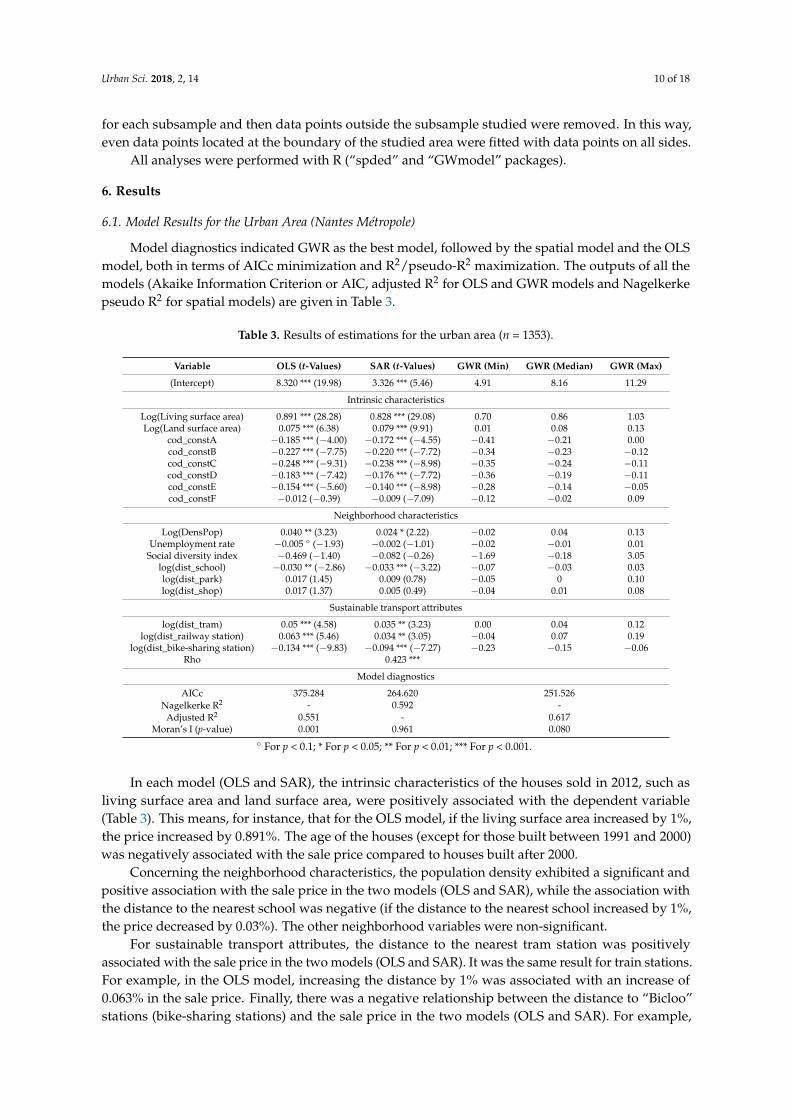
Model diagnostics indicated GWR as the best model, followed by the spatial model and the OLSmodel, both in terms of AICc minimization and R2/pseudo-R2 maximization. The outputs of all themodels (Akaike Information Criterion or AIC, adjusted R2 for OLS and GWR models and Nagelkerkepseudo R2 for spatial models) are given in Table 3.
Table 3. Results of estimations for the urban area (n = 1353).
Variable OLS (t-Values) SAR (t-Values) GWR (Min) GWR (Median) GWR (Max)
(Intercept) 8.320 *** (19.98) 3.326 *** (5.46) 4.91 8.16 11.29
Intrinsic characteristics
Log(Living surface area) 0.891 *** (28.28) 0.828 *** (29.08) 0.70 0.86 1.03Log(Land surface area) 0.075 *** (6.38) 0.079 *** (9.91) 0.01 0.08 0.13
cod_constA −0.185 *** (−4.00) −0.172 *** (−4.55) −0.41 −0.21 0.00cod_constB −0.227 *** (−7.75) −0.220 *** (−7.72) −0.34 −0.23 −0.12cod_constC −0.248 *** (−9.31) −0.238 *** (−8.98) −0.35 −0.24 −0.11cod_constD −0.183 *** (−7.42) −0.176 *** (−7.72) −0.36 −0.19 −0.11cod_constE −0.154 *** (−5.60) −0.140 *** (−8.98) −0.28 −0.14 −0.05cod_constF −0.012 (−0.39) −0.009 (−7.09) −0.12 −0.02 0.09
Neighborhood characteristics
Log(DensPop) 0.040 ** (3.23) 0.024 * (2.22) −0.02 0.04 0.13Unemployment rate −0.005 ◦ (−1.93) −0.002 (−1.01) −0.02 −0.01 0.01
Social diversity index −0.469 (−1.40) −0.082 (−0.26) −1.69 −0.18 3.05log(dist_school) −0.030 ** (−2.86) −0.033 *** (−3.22) −0.07 −0.03 0.03log(dist_park) 0.017 (1.45) 0.009 (0.78) −0.05 0 0.10log(dist_shop) 0.017 (1.37) 0.005 (0.49) −0.04 0.01 0.08
Sustainable transport attributes
log(dist_tram) 0.05 *** (4.58) 0.035 ** (3.23) 0.00 0.04 0.12log(dist_railway station) 0.063 *** (5.46) 0.034 ** (3.05) −0.04 0.07 0.19
log(dist_bike-sharing station) −0.134 *** (−9.83) −0.094 *** (−7.27) −0.23 −0.15 −0.06Rho 0.423 ***
Model diagnostics
AICc 375.284 264.620 251.526Nagelkerke R2 - 0.592 -
Adjusted R2 0.551 - 0.617Moran’s I (p-value) 0.001 0.961 0.080
◦ For p < 0.1; * For p < 0.05; ** For p < 0.01; *** For p < 0.001.
In each model (OLS and SAR), the intrinsic characteristics of the houses sold in 2012, such asliving surface area and land surface area, were positively associated with the dependent variable(Table 3). This means, for instance, that for the OLS model, if the living surface area increased by 1%,the price increased by 0.891%. The age of the houses (except for those built between 1991 and 2000)was negatively associated with the sale price compared to houses built after 2000.
Concerning the neighborhood characteristics, the population density exhibited a significant andpositive association with the sale price in the two models (OLS and SAR), while the association withthe distance to the nearest school was negative (if the distance to the nearest school increased by 1%,the price decreased by 0.03%). The other neighborhood variables were non-significant.
For sustainable transport attributes, the distance to the nearest tram station was positivelyassociated with the sale price in the two models (OLS and SAR). It was the same result for train stations.For example, in the OLS model, increasing the distance by 1% was associated with an increase of0.063% in the sale price. Finally, there was a negative relationship between the distance to “Bicloo”stations (bike-sharing stations) and the sale price in the two models (OLS and SAR). For example,
Urban Sci. 2018, 2, 14 11 of 18
in the OLS model, increasing the distance by 1% was associated with a decrease of 0.134%. Note that inall the previous and following models, the magnitude of such relationships is valid only for a marginalvariation in the variable values, i.e., in the small vicinity of the observed transaction.
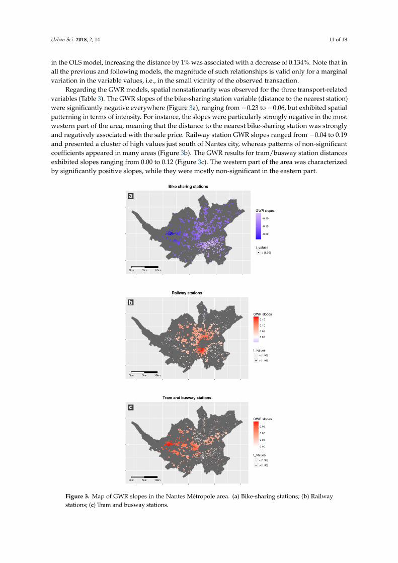
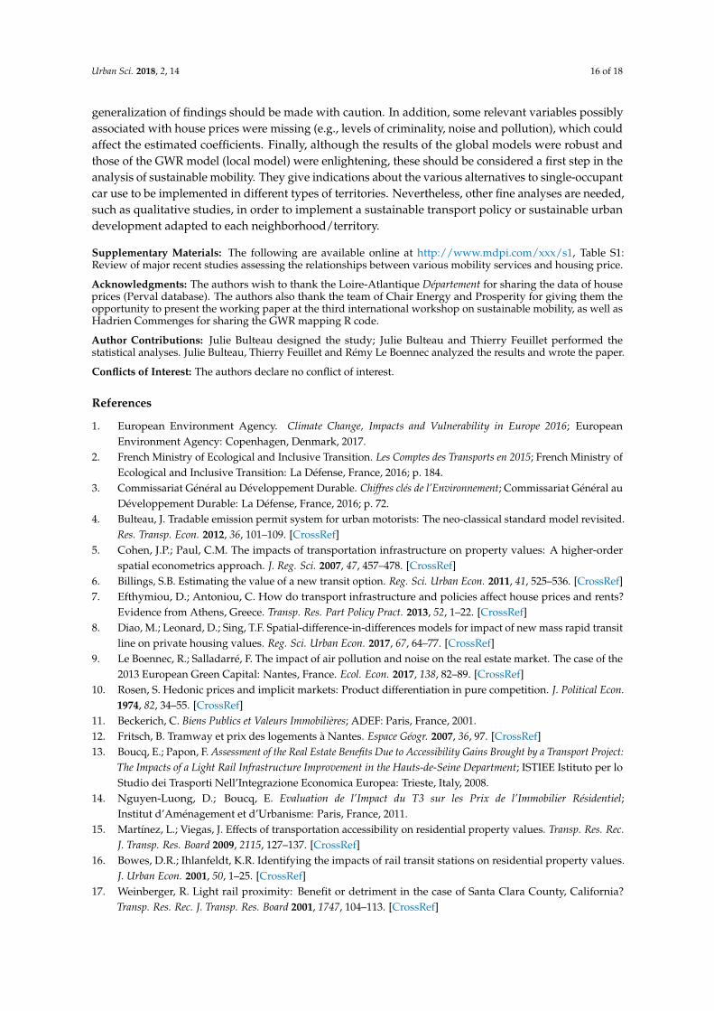
Regarding the GWR models, spatial nonstationarity was observed for the three transport-relatedvariables (Table 3). The GWR slopes of the bike-sharing station variable (distance to the nearest station)were significantly negative everywhere (Figure 3a), ranging from −0.23 to −0.06, but exhibited spatialpatterning in terms of intensity. For instance, the slopes were particularly strongly negative in the mostwestern part of the area, meaning that the distance to the nearest bike-sharing station was stronglyand negatively associated with the sale price. Railway station GWR slopes ranged from −0.04 to 0.19and presented a cluster of high values just south of Nantes city, whereas patterns of non-significantcoefficients appeared in many areas (Figure 3b). The GWR results for tram/busway station distancesexhibited slopes ranging from 0.00 to 0.12 (Figure 3c). The western part of the area was characterizedby significantly positive slopes, while they were mostly non-significant in the eastern part.
Urban Sci. 2018, 2, x FOR PEER REVIEW 11 of 18
“Bicloo” stations (bike-sharing stations) and the sale price in the two models (OLS and SAR). For example, in the OLS model, increasing the distance by 1% was associated with a decrease of 0.134%. Note that in all the previous and following models, the magnitude of such relationships is valid only for a marginal variation in the variable values, i.e., in the small vicinity of the observed transaction.
Regarding the GWR models, spatial nonstationarity was observed for the three transport-related variables (Table 3). The GWR slopes of the bike-sharing station variable (distance to the nearest station) were significantly negative everywhere (Figure 3a), ranging from −0.23 to −0.06, but exhibited spatial patterning in terms of intensity. For instance, the slopes were particularly strongly negative in the most western part of the area, meaning that the distance to the nearest bike-sharing station was strongly and negatively associated with the sale price. Railway station GWR slopes ranged from −0.04 to 0.19 and presented a cluster of high values just south of Nantes city, whereas patterns of non-significant coefficients appeared in many areas (Figure 3b). The GWR results for tram/busway station distances exhibited slopes ranging from 0.00 to 0.12 (Figure 3c). The western part of the area was characterized by significantly positive slopes, while they were mostly non-significant in the eastern part.
Figure 3. Map of GWR slopes in the Nantes Métropole area. (a) Bike-sharing stations; (b) Railway stations; (c) Tram and busway stations.
Figure 3. Map of GWR slopes in the Nantes Métropole area. (a) Bike-sharing stations; (b) Railwaystations; (c) Tram and busway stations.
Urban Sci. 2018, 2, 14 12 of 18
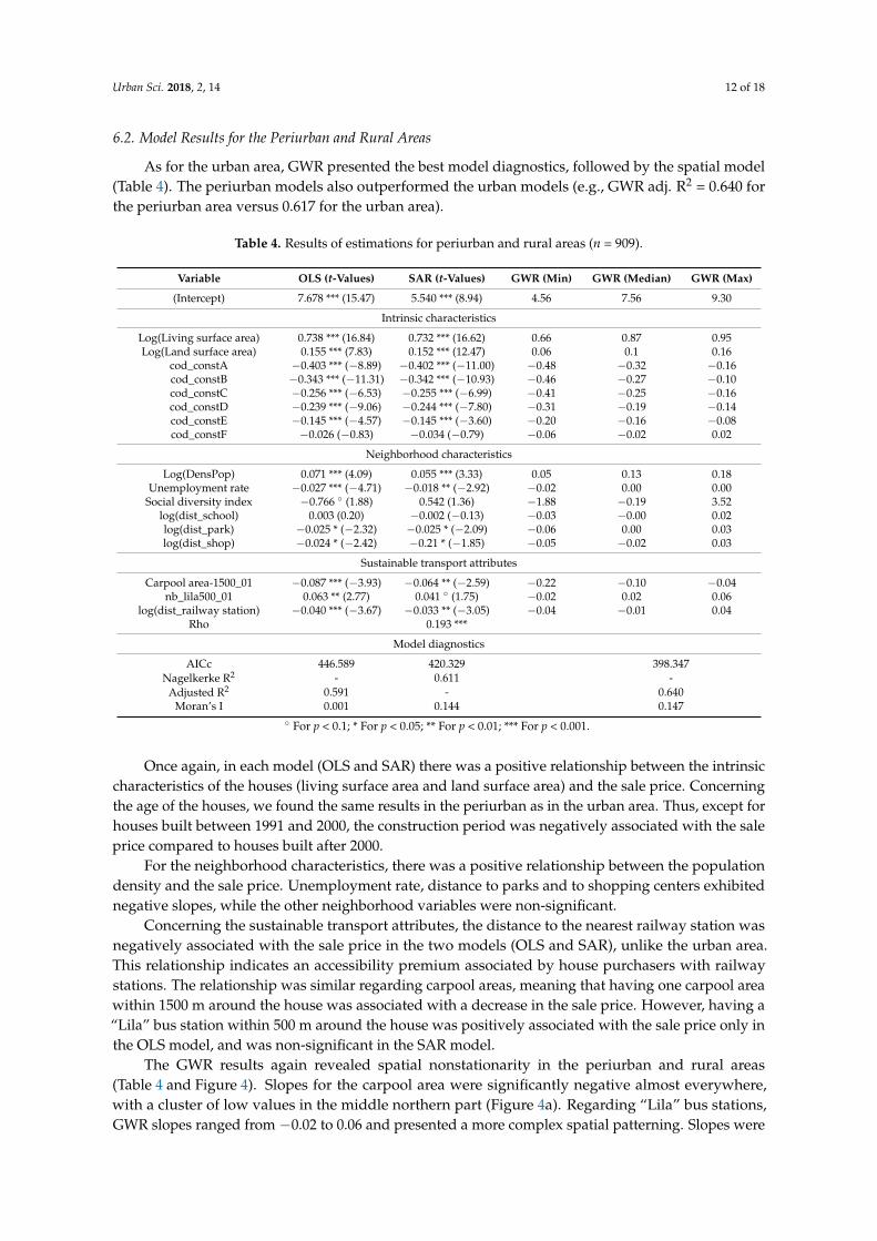
6.2. Model Results for the Periurban and Rural Areas
As for the urban area, GWR presented the best model diagnostics, followed by the spatial model(Table 4). The periurban models also outperformed the urban models (e.g., GWR adj. R2 = 0.640 forthe periurban area versus 0.617 for the urban area).
Table 4. Results of estimations for periurban and rural areas (n = 909).
Variable OLS (t-Values) SAR (t-Values) GWR (Min) GWR (Median) GWR (Max)
(Intercept) 7.678 *** (15.47) 5.540 *** (8.94) 4.56 7.56 9.30
Intrinsic characteristics
Log(Living surface area) 0.738 *** (16.84) 0.732 *** (16.62) 0.66 0.87 0.95Log(Land surface area) 0.155 *** (7.83) 0.152 *** (12.47) 0.06 0.1 0.16
cod_constA −0.403 *** (−8.89) −0.402 *** (−11.00) −0.48 −0.32 −0.16cod_constB −0.343 *** (−11.31) −0.342 *** (−10.93) −0.46 −0.27 −0.10cod_constC −0.256 *** (−6.53) −0.255 *** (−6.99) −0.41 −0.25 −0.16cod_constD −0.239 *** (−9.06) −0.244 *** (−7.80) −0.31 −0.19 −0.14cod_constE −0.145 *** (−4.57) −0.145 *** (−3.60) −0.20 −0.16 −0.08cod_constF −0.026 (−0.83) −0.034 (−0.79) −0.06 −0.02 0.02
Neighborhood characteristics
Log(DensPop) 0.071 *** (4.09) 0.055 *** (3.33) 0.05 0.13 0.18Unemployment rate −0.027 *** (−4.71) −0.018 ** (−2.92) −0.02 0.00 0.00
Social diversity index −0.766 ◦ (1.88) 0.542 (1.36) −1.88 −0.19 3.52log(dist_school) 0.003 (0.20) −0.002 (−0.13) −0.03 −0.00 0.02log(dist_park) −0.025 * (−2.32) −0.025 * (−2.09) −0.06 0.00 0.03log(dist_shop) −0.024 * (−2.42) −0.21 * (−1.85) −0.05 −0.02 0.03
Sustainable transport attributes
Carpool area-1500_01 −0.087 *** (−3.93) −0.064 ** (−2.59) −0.22 −0.10 −0.04nb_lila500_01 0.063 ** (2.77) 0.041 ◦ (1.75) −0.02 0.02 0.06
log(dist_railway station) −0.040 *** (−3.67) −0.033 ** (−3.05) −0.04 −0.01 0.04Rho 0.193 ***
Model diagnostics
AICc 446.589 420.329 398.347Nagelkerke R2 - 0.611 -
Adjusted R2 0.591 - 0.640Moran’s I 0.001 0.144 0.147
◦ For p < 0.1; * For p < 0.05; ** For p < 0.01; *** For p < 0.001.
Once again, in each model (OLS and SAR) there was a positive relationship between the intrinsiccharacteristics of the houses (living surface area and land surface area) and the sale price. Concerningthe age of the houses, we found the same results in the periurban as in the urban area. Thus, except forhouses built between 1991 and 2000, the construction period was negatively associated with the saleprice compared to houses built after 2000.
For the neighborhood characteristics, there was a positive relationship between the populationdensity and the sale price. Unemployment rate, distance to parks and to shopping centers exhibitednegative slopes, while the other neighborhood variables were non-significant.
Concerning the sustainable transport attributes, the distance to the nearest railway station wasnegatively associated with the sale price in the two models (OLS and SAR), unlike the urban area.This relationship indicates an accessibility premium associated by house purchasers with railwaystations. The relationship was similar regarding carpool areas, meaning that having one carpool areawithin 1500 m around the house was associated with a decrease in the sale price. However, having a“Lila” bus station within 500 m around the house was positively associated with the sale price only inthe OLS model, and was non-significant in the SAR model.
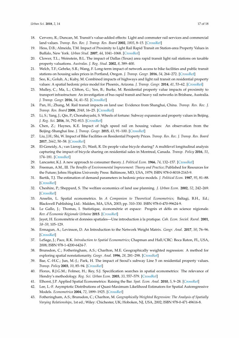
The GWR results again revealed spatial nonstationarity in the periurban and rural areas(Table 4 and Figure 4). Slopes for the carpool area were significantly negative almost everywhere,with a cluster of low values in the middle northern part (Figure 4a). Regarding “Lila” bus stations,GWR slopes ranged from −0.02 to 0.06 and presented a more complex spatial patterning. Slopes were

Urban Sci. 2018, 2, 14 13 of 18
significant in the northern part of the periurban area, but mostly non-significant elsewhere, except ina few southern sectors (Figure 4b). Finally, the results for the distance to a railway station mainlyrevealed non-significant slopes, except in the middle and northwestern part with significant negativevalues (Figure 4c).
Urban Sci. 2018, 2, x FOR PEER REVIEW 13 of 18
slopes ranged from −0.02 to 0.06 and presented a more complex spatial patterning. Slopes were significant in the northern part of the periurban area, but mostly non-significant elsewhere, except in a few southern sectors (Figure 4b). Finally, the results for the distance to a railway station mainly revealed non-significant slopes, except in the middle and northwestern part with significant negative values (Figure 4c).
Figure 4. Map of GWR slopes in periurban and rural areas. (a) Carpool areas; (b) “Lila” bus stations; (c) Railway stations.
7. Discussion
In 2004, Time Magazine named Nantes “the most liveable city in Europe” and in 2013 it held the title of European Green Capital. Over the past 10 years, Nantes has been developing a sustainable transport policy with a focus on public transport and cycling [45]. In this study, we sought to explore whether the proximity to alternative offers to the private car affected house prices, not only in the urban area but also in periurban and rural areas.
Our results from the two samples (urban and periurban/rural areas) showed that the intrinsic characteristics of the house (living surface area and land surface area) were positively associated with the sale price. These results are consistent with other works (e.g., [46]). The population density also
Figure 4. Map of GWR slopes in periurban and rural areas. (a) Carpool areas; (b) “Lila” bus stations;(c) Railway stations.
7. Discussion
In 2004, Time Magazine named Nantes “the most liveable city in Europe” and in 2013 it held thetitle of European Green Capital. Over the past 10 years, Nantes has been developing a sustainabletransport policy with a focus on public transport and cycling [45]. In this study, we sought to explorewhether the proximity to alternative offers to the private car affected house prices, not only in theurban area but also in periurban and rural areas.
Our results from the two samples (urban and periurban/rural areas) showed that the intrinsiccharacteristics of the house (living surface area and land surface area) were positively associatedwith the sale price. These results are consistent with other works (e.g., [46]). The population density
Urban Sci. 2018, 2, 14 14 of 18
also exhibited the expected relationships. Indeed, Saulnier [47] found the same results for the cityof Grenoble.
7.1. Urban Area (Nantes Métropole)
In the urban area, three sustainable transport solutions were studied: tramways and the busway(BRT), railway stations and the bike-sharing system. We observed a positive association betweenthe distance to the nearest tram station and the house prices in the two global models (OLS andSAR). According to Bowes and Ihlanfeldt [16], if station proximity has no effect or a negative effect onproperty values, the importance of the negative externalities emitted by the station are emphasized asan offsetting or dominant factor. Thus, it seems evident that the negative externalities of tramways andthe busway (noise for example) have a negative impact on house prices [7,9,48]. However, the GWRmodel provided important information that questions this global result. Indeed, there were a fewlocal differences in the impact of the tramway and busway infrastructure on the sale price (Figure 3c).We observed spatial nonstationarity for the tramway and busway variables. For example, the westernpart of the urban area was characterized by significantly positive slopes, while they were mostlynon-significant in the eastern part. These results show that the tramway infrastructure did not havethe same impact within the urban area. This can be seen as an indication to implement local transportpolicy. For example, the district of Bellevue in the western part of the urban area may need someadditional funding to improve its image in the eyes of the potential house purchasers. In the frameworkof an enlarged urban renewal policy, this may yield even wider positive effects if wealthier householdssettle in the neighborhood.
The same positive relationship between the distance to nearest railway station and the sale pricewas observed in the global models (OLS and SAR). Once again, these results are consistent with otherhedonic price studies, such as Bowes and Ihlanfeldt [16] and Seo et al. [22], which found that proximityto transportation infrastructure can reduce property values; this may be due to different nuisances(crime, noise and air pollution) associated with proximity to these facilities. However, this global resultneeds to be put into perspective because in the local model (GWR model), this relationship varied inthe urban area. Indeed, the GWR slopes for the distance to the nearest railway station ranged from−0.04 to 0.19 (Table 3) and presented a cluster of high values just south of Nantes city, whereas patternsof non-significant coefficients appeared in many areas. The quality of the 2nd and 4th tramline/buswayservices (notably their frequency and time range) for the inhabitants of this area located close to thecity center makes it superfluous to choose a house near a railway station, whereas the different typesof nuisance remain [12].
Finally, the distance to the nearest “Bicloo” station (bike-sharing station) was negatively associatedwith house prices in the two models (OLS and SAR). In addition, the GWR model showed thatthis association exhibited spatial patterning in terms of intensity. Our results are consistent withEl-Geneidy et al. [28] who found that the presence of a bike-sharing system is expected to increaseproperty values. The authors concluded that policy makers could improve the local environment andbenefit from economic gains in developing bike-sharing systems, as this transport policy could be inrelation to higher property values, health benefits and greater welfare for residents.
7.2. Periurban and Rural Areas
In the periurban and rural areas, we focused on three sustainable transport systems: railwaystations, carpool areas and “Lila” bus stations. The distance to the nearest railway station wasnegatively associated with house prices in the two global models. It is worth noting that thiscorresponds to a sign reversal compared to the urban area. This could be due to the fact that inurban areas, negative externalities associated with train stations (e.g., noise) outweigh the serviceprovided, while in rural areas, having a train station not too far implies a significant gain in accessibility.In the periurban/rural areas, however, the matter is more complex than appears at first sight and waselucidated with the GWR model. In fact, the distance to the nearest railway station mainly revealed
Urban Sci. 2018, 2, 14 15 of 18
non-significant slopes, except in the middle and northeastern part with significant negative values(Figure 4c). In those areas, being located near a railway station of the Châteaubriant-Nantes line(North) or the Ancenis-Nantes line (East) significantly improves overall accessibility to Nantes; in thefirst case, because of the lack of alternative public transit offers in this relatively low-density periurbanarea and, in the second case, because of the intrinsic quality of the train line service, which providesdaily commuters with a 16 min trip for a 43 km distance.
The availability of a carpool area in the house vicinity was significant in the two global models.Having at least one carpool area in a buffer of 1500 m around a house located in the periurbanand rural areas was associated with a decrease of 8.7% (OLS) and 6.4% (SAR) in the sale price.Nevertheless, the GWR model exhibited slopes for carpool area ranging from −0.22 to −0.04 and wassignificant almost everywhere, with a cluster of low values in the middle northern part (Figure 4a).This result may be considered jointly with the proximity of the time-competitive Nantes-Ancenis(Northeast) railway line, which may be preferred to carpooling by daily commuters to Nantes citycenter. In the northern part, the “Lila” bus offer may be considered cheaper by poorer households thanin the rest of the periurban and rural areas (unique ticket cost of €2 in 2012). Furthermore, the effectiveuse of carpooling in 2012 was not as developed as it has since become, in particular for short andmedium-distance trips, reinforcing the households’ propensity to use alternative modes when theyexist. The results are difficult to compare with other studies since, to our knowledge, there have beennone on hedonic prices and carpool areas.
The “Lila” bus station, which was specified as at least one “Lila” bus station in a buffer of 500 mradius around the house located in the periurban and rural areas, exhibited a positive relationshipwith the sale price in the OLS model and became non-significant in the SAR model. The GWR modelpresented a more complex spatial patterning. Slopes were significant in the northern part of the area,but mostly non-significant elsewhere, except in a few southern sectors. This pattern is consistentwith the absence of alternative modes in the northern area until 2014 and the Châteaubriant-Nantesrailway line, with the exception of carpool areas that were potentially under-utilized in 2012. In thesoutheastern part of the periurban and rural areas, the “Lila” lines may be viewed as attractive byparents with children going to middle or high school within the urban area.
8. Conclusions
The objective of this paper was twofold: (i) to explore the relationships between several sustainabletransportation infrastructures and the sale price of houses in urban and periurban/rural areasof Nantes and (ii) to derive from these analyses useful elements to help policy-makers reducesingle-occupant car use. To achieve this, we used the hedonic price method and spatial econometricmodels (SAR and GWR).
The major finding of this study is that some sustainable transportation solutions had no orcounterintuitive relationships with house prices but, above all, that these results exhibited spatialvariations throughout the study area. We highlighted a territorial heterogeneity at two differentscales. For example, in the urban area, the distance to the nearest tramway station was positivelyassociated with house prices in the global model, but our GWR results showed that this associationvaried according to the place within the urban territory. The same rationale could be applied regardingthe bike-sharing stations. This could serve as a useful indicator to implement local transport/mobilityoffers in sufficiently dense areas; in return, it could assist the design of urban planning policies to theextent that building housing near pre-existing mobility offers could prove profitable. In the same way,in the periurban and rural areas, the “Lila” bus station proximity was positively associated with theproperty sale price in the two global models but, once again, our GWR results showed a more complexspatial patterning. These results imply a spatial adaptation of transport policies and therefore differentsolutions to achieve sustainable mobility throughout the territories.
The main limitation of this study relates to the cross-sectional nature of the analyses, which doesnot allow for causal inference. Our results are also specific to this area and these data, so that any
Urban Sci. 2018, 2, 14 16 of 18
generalization of findings should be made with caution. In addition, some relevant variables possiblyassociated with house prices were missing (e.g., levels of criminality, noise and pollution), which couldaffect the estimated coefficients. Finally, although the results of the global models were robust andthose of the GWR model (local model) were enlightening, these should be considered a first step in theanalysis of sustainable mobility. They give indications about the various alternatives to single-occupantcar use to be implemented in different types of territories. Nevertheless, other fine analyses are needed,such as qualitative studies, in order to implement a sustainable transport policy or sustainable urbandevelopment adapted to each neighborhood/territory.
Supplementary Materials: The following are available online at http://www.mdpi.com/xxx/s1, Table S1:Review of major recent studies assessing the relationships between various mobility services and housing price.
Acknowledgments: The authors wish to thank the Loire-Atlantique Département for sharing the data of houseprices (Perval database). The authors also thank the team of Chair Energy and Prosperity for giving them theopportunity to present the working paper at the third international workshop on sustainable mobility, as well asHadrien Commenges for sharing the GWR mapping R code.
Author Contributions: Julie Bulteau designed the study; Julie Bulteau and Thierry Feuillet performed thestatistical analyses. Julie Bulteau, Thierry Feuillet and Rémy Le Boennec analyzed the results and wrote the paper.
Conflicts of Interest: The authors declare no conflict of interest.
References
1. European Environment Agency. Climate Change, Impacts and Vulnerability in Europe 2016; EuropeanEnvironment Agency: Copenhagen, Denmark, 2017.
2. French Ministry of Ecological and Inclusive Transition. Les Comptes des Transports en 2015; French Ministry ofEcological and Inclusive Transition: La Défense, France, 2016; p. 184.
3. Commissariat Général au Développement Durable. Chiffres clés de l’Environnement; Commissariat Général auDéveloppement Durable: La Défense, France, 2016; p. 72.
4. Bulteau, J. Tradable emission permit system for urban motorists: The neo-classical standard model revisited.Res. Transp. Econ. 2012, 36, 101–109. [CrossRef]
5. Cohen, J.P.; Paul, C.M. The impacts of transportation infrastructure on property values: A higher-orderspatial econometrics approach. J. Reg. Sci. 2007, 47, 457–478. [CrossRef]
6. Billings, S.B. Estimating the value of a new transit option. Reg. Sci. Urban Econ. 2011, 41, 525–536. [CrossRef]7. Efthymiou, D.; Antoniou, C. How do transport infrastructure and policies affect house prices and rents?
Evidence from Athens, Greece. Transp. Res. Part Policy Pract. 2013, 52, 1–22. [CrossRef]8. Diao, M.; Leonard, D.; Sing, T.F. Spatial-difference-in-differences models for impact of new mass rapid transit
line on private housing values. Reg. Sci. Urban Econ. 2017, 67, 64–77. [CrossRef]9. Le Boennec, R.; Salladarré, F. The impact of air pollution and noise on the real estate market. The case of the
2013 European Green Capital: Nantes, France. Ecol. Econ. 2017, 138, 82–89. [CrossRef]10. Rosen, S. Hedonic prices and implicit markets: Product differentiation in pure competition. J. Political Econ.
1974, 82, 34–55. [CrossRef]11. Beckerich, C. Biens Publics et Valeurs Immobilières; ADEF: Paris, France, 2001.12. Fritsch, B. Tramway et prix des logements à Nantes. Espace Géogr. 2007, 36, 97. [CrossRef]13. Boucq, E.; Papon, F. Assessment of the Real Estate Benefits Due to Accessibility Gains Brought by a Transport Project:
The Impacts of a Light Rail Infrastructure Improvement in the Hauts-de-Seine Department; ISTIEE Istituto per loStudio dei Trasporti Nell’Integrazione Economica Europea: Trieste, Italy, 2008.
14. Nguyen-Luong, D.; Boucq, E. Evaluation de l’Impact du T3 sur les Prix de l’Immobilier Résidentiel;Institut d’Aménagement et d’Urbanisme: Paris, France, 2011.
15. Martínez, L.; Viegas, J. Effects of transportation accessibility on residential property values. Transp. Res. Rec.J. Transp. Res. Board 2009, 2115, 127–137. [CrossRef]
16. Bowes, D.R.; Ihlanfeldt, K.R. Identifying the impacts of rail transit stations on residential property values.J. Urban Econ. 2001, 50, 1–25. [CrossRef]
17. Weinberger, R. Light rail proximity: Benefit or detriment in the case of Santa Clara County, California?Transp. Res. Rec. J. Transp. Res. Board 2001, 1747, 104–113. [CrossRef]
Urban Sci. 2018, 2, 14 17 of 18
18. Cervero, R.; Duncan, M. Transit’s value-added effects: Light and commuter rail services and commercialland values. Transp. Res. Rec. J. Transp. Res. Board 2002, 1805, 8–15. [CrossRef]
19. Hess, D.B.; Almeida, T.M. Impact of Proximity to Light Rail Rapid Transit on Station-area Property Values inBuffalo, New York. Urban Stud. 2007, 44, 1041–1068. [CrossRef]
20. Clower, T.L.; Weinstein, B.L. The impact of Dallas (Texas) area rapid transit light rail stations on taxableproperty valuations. Australas. J. Reg. Stud. 2002, 8, 389–400.
21. Welch, T.F.; Gehrke, S.R.; Wang, F. Long-term impact of network access to bike facilities and public transitstations on housing sales prices in Portland, Oregon. J. Transp. Geogr. 2016, 54, 264–272. [CrossRef]
22. Seo, K.; Golub, A.; Kuby, M. Combined impacts of highways and light rail transit on residential propertyvalues: A spatial hedonic price model for Phoenix, Arizona. J. Transp. Geogr. 2014, 41, 53–62. [CrossRef]
23. Mulley, C.; Ma, L.; Clifton, G.; Yen, B.; Burke, M. Residential property value impacts of proximity totransport infrastructure: An investigation of bus rapid transit and heavy rail networks in Brisbane, Australia.J. Transp. Geogr. 2016, 54, 41–52. [CrossRef]
24. Pan, H.; Zhang, M. Rail transit impacts on land use: Evidence from Shanghai, China. Transp. Res. Rec. J.Transp. Res. Board 2008, 2048, 16–25. [CrossRef]
25. Li, S.; Yang, J.; Qin, P.; Chonabayashi, S. Wheels of fortune: Subway expansion and property values in Beijing.J. Reg. Sci. 2016, 56, 792–813. [CrossRef]
26. Chen, Z.; Haynes, K.E. Impact of high speed rail on housing values: An observation from theBeijing–Shanghai line. J. Transp. Geogr. 2015, 43, 91–100. [CrossRef]
27. Liu, J.H.; Shi, W. Impact of Bike Facilities on Residential Property Prices. Transp. Res. Rec. J. Transp. Res. Board2017, 2662, 50–58. [CrossRef]
28. El-Geneidy, A.; van Lierop, D.; Wasfi, R. Do people value bicycle sharing? A multilevel longitudinal analysiscapturing the impact of bicycle sharing on residential sales in Montreal, Canada. Transp. Policy 2016, 51,174–181. [CrossRef]
29. Lancaster, K.J. A new approach to consumer theory. J. Political Econ. 1966, 74, 132–157. [CrossRef]30. Freeman, A.M., III. The Benefits of Environmental Improvement: Theory and Practice; Published for Resources for
the Future; Johns Hopkins University Press: Baltimore, MD, USA, 1979; ISBN 978-0-8018-2163-9.31. Bartik, T.J. The estimation of demand parameters in hedonic price models. J. Political Econ. 1987, 95, 81–88.
[CrossRef]32. Cheshire, P.; Sheppard, S. The welfare economics of land use planning. J. Urban Econ. 2002, 52, 242–269.
[CrossRef]33. Anselin, L. Spatial econometrics. In A Companion to Theoretical Econometrics; Baltagi, B.H., Ed.;
Blackwell Publishing Ltd.: Malden, MA, USA, 2003; pp. 310–330. ISBN 978-0-470-99624-9.34. Le Gallo, J.; Thomas, I. Statistique, économétrie et espace: Progrès et défis en science régionale.
Rev. d’Économie Régionale Urbaine 2015. [CrossRef]35. Jayet, H. Econométrie et données spatiales—Une introduction à la pratique. Cah. Econ. Sociol. Rural. 2001,
58–59, 105–129.36. Ermagun, A.; Levinson, D. An Introduction to the Network Weight Matrix. Geogr. Anal. 2017, 50, 76–96.
[CrossRef]37. LeSage, J.; Pace, R.K. Introduction to Spatial Econometrics; Chapman and Hall/CRC: Boca Raton, FL, USA,
2008; ISBN 978-1-4200-6424-7.38. Brunsdon, C.; Fotheringham, A.S.; Charlton, M.E. Geographically weighted regression: A method for
exploring spatial nonstationarity. Geogr. Anal. 1996, 28, 281–298. [CrossRef]39. Bae, C.-H.C.; Jun, M.-J.; Park, H. The impact of Seoul’s subway Line 5 on residential property values.
Transp. Policy 2003, 10, 85–94. [CrossRef]40. Florax, R.J.G.M.; Folmer, H.; Rey, S.J. Specification searches in spatial econometrics: The relevance of
Hendry’s methodology. Reg. Sci. Urban Econ. 2003, 33, 557–579. [CrossRef]41. Elhorst, J.P. Applied Spatial Econometrics: Raising the Bar. Spat. Econ. Anal. 2010, 5, 9–28. [CrossRef]42. Lee, L.-F. Asymptotic Distributions of Quasi-Maximum Likelihood Estimators for Spatial Autoregressive
Models. Econometrica 2004, 72, 1899–1925. [CrossRef]43. Fotheringham, A.S.; Brunsdon, C.; Charlton, M. Geographically Weighted Regression: The Analysis of Spatially
Varying Relationships, 1st ed.; Wiley: Chichester, UK; Hoboken, NJ, USA, 2002; ISBN 978-0-471-49616-8.

Urban Sci. 2018, 2, 14 18 of 18
44. Feuillet, T.; Charreire, H.; Menai, M.; Salze, P.; Simon, C.; Dugas, J.; Hercberg, S.; Andreeva, V.A.; Enaux, C.;Weber, C.; et al. Spatial heterogeneity of the relationships between environmental characteristics and activecommuting: Towards a locally varying social ecological model. Int. J. Health Geogr. 2015, 14. [CrossRef][PubMed]
45. European Commission. 2013. Available online: http://ec.europa.eu/environment/europeangreencapital/winning-cities/2013-nantes/ (accessed on 10 September 2017).
46. Bureau, B.; Glachant, M. Évaluation de l’impact des politiques, assessing the Impact of “Green Neighborhood”and “Quiet Neighborhood” Policies on Paris Property Values. Econ. Prévis. 2010, 1, 27–44.
47. Saulnier, J. Une Application des Prix Hédonistes: Influence de la Qualité de l’Air sur le Prix des Logements?Available online: http://prodinra.inra.fr/?locale=fr#!ConsultNotice:150792 (accessed on 1 November 2017).
48. Wagner, G.A.; Komarek, T.; Martin, J. Is the light rail “Tide” lifting property values? Evidence from HamptonRoads, VA. Reg. Sci. Urban Econ. 2017, 65, 25–37. [CrossRef]
© 2018 by the authors. Licensee MDPI, Basel, Switzerland. This article is an open accessarticle distributed under the terms and conditions of the Creative Commons Attribution(CC BY) license (http://creativecommons.org/licenses/by/4.0/).